


Introduction
A candidate in a Single Member Plurality (SMP) system wins a seat if they receive the plurality of votes in a local election. Given the rise of political parties and their centrality in Canada’s parliamentary system (Godbout, Reference Godbout2020), the ultimate outcome of the election—who controls the government—is determined by the party (or parties) whose candidates win a majority of these contests (Gudgin, Reference Gudgin1979). In this way, it matters to parties not just how many votes they receive, but also where the party receives these votes (Cairns, Reference Cairns1968). Parties can, and often do, win more seats than their opponents despite receiving fewer votes overall. Geography is inherent to the Canadian electoral system (Johnston, Reference Johnston2017).
In a country as geographically large and diverse as Canada (Schwartz, Reference Schwartz1974), it is reasonable to integrate expressions of local preferences into the electoral process, not least because of the threat of an alienated minority representing a majority of citizens in contiguous localities revolting, as in the Red River and North-West rebellions in the late nineteenth century, or even separating to form a new country, as Quebec nearly did in the late twentieth century. Thus, let us acknowledge that territorial representation is a reasonable objective of the Canadian electoral system. It is one thing, however, for a party to win an election because of the territorial distribution of its support across the country, and a different thing for a party to win because of where the lines between electoral districts happened to be drawn. The former is a type of local representation, whereas the latter is an electoral district boundary effect.
The extreme example of gerrymandering makes clear the distinction between “local representation” and “electoral district boundary effects.” Yet, the distinction also raises a more general normative question beyond gerrymandering: to what extent can we interpret Canadian election outcomes as the expression of local plurality preferences of voters across the country, as we have tended to do at least since Cairns (Reference Cairns1968), and to what extent must we also interpret the outcomes as sensitive to the particular configuration of boundaries that happened to be drawn between electoral districts within the same areas?
The answer to this question has practical implications, also. If the only thing that matters for parties vis-a-vis election outcomes is the level and territorial distribution of their vote, then we should expect to see parties responding to these strategic imperatives (Cairns, Reference Cairns1968). As Johnston and Ballantyne (Reference Johnston and Ballantyne1977) explained, a party seeking to form a government will need to make regional appeals in enough places to win a majority of the seats (which is arguably the nationalizing effect an SMP system intends to produce in the winning party). Large parties that focus too heavily in one place will produce many so-called “wasted votes” and lose the election. By the same token, we should expect to see smaller parties rewarded when they focus their efforts in few places, as they can win more seats from their small share of the vote than if this same level of support was spread more evenly across the country (Johnston and Ballantyne, Reference Johnston and Ballantyne1977). In this way, the system rewards regionally concentrated minority preferences at the expense of diffuse minority preferences. Despite the differences between the strategic imperatives facing large and small parties, notice how both strategies involve campaigning for the support of voters, and they are also both consistent with the separate albeit conflicting principles of Canada’s political system more generally—that is, “universalism” and “particularism” (LaSelva, Reference LaSelva1996: 18).
But what happens if election outcomes are highly sensitive to the positions of boundaries? In this scenario, we should expect to see parties jostling for strategic advantage not only by attempting to secure the support of particular voters during elections, but also by attempting to influence the design of electoral district boundaries to tilt elections in their favour (Mattingly and Vaughn, Reference Mattingly and Vaughn2014: 15). Until recently, this was mostly a theoretical and political concern with few if any practical implications for Canadian elections. To be sure, parties routinely preoccupied themselves with attempts to gerrymander before the middle of the twentieth century, but they lacked the technical capacity to do so effectively (Carty, Reference Carty1985; Dawson, Reference Dawson1935; Ward, Reference Ward1950). There are more possible ways to sort Canadian voters into hundreds of districts than there are atoms in the observable universe (Clark et al., Reference Clark, Glenn, Lee and Villar2025: 2), and there are more allowable ways to sort them than there are atoms in the galaxy (Donnay and Kahle, Reference Donnay and Kahle2024). For reference, there are approximately seven octillion atoms in the human body, which is $7 \times {10^{27}}$
or seven million billion trillions. Gerrymandering attempts were thwarted by the lack of quality data and the technology necessary to manage anything like complexity of this magnitude, which meant that gerrymanders often ended up benefitting their opponents as much as they benefitted themselves (Courtney, Reference Courtney2001: 20; Dawson, Reference Dawson1935: 215; Ward, Reference Ward1950: 28). When the power to design electoral district boundaries was finally delegated to non-partisan boundary commissions in 1964, politicians continued to lobby at the margins for advantageous boundaries in specific locales (Eagles and Carty, Reference Eagles and Carty1999: 89), but they still lacked the technical capacity to strategize effectively at the scale of the electoral system as a whole (Carty, Reference Carty1985: 275), or to fully understand the implications of the boundaries that were ultimately drawn by the non-partisan commissions.
$7 \times {10^{27}}$
or seven million billion trillions. Gerrymandering attempts were thwarted by the lack of quality data and the technology necessary to manage anything like complexity of this magnitude, which meant that gerrymanders often ended up benefitting their opponents as much as they benefitted themselves (Courtney, Reference Courtney2001: 20; Dawson, Reference Dawson1935: 215; Ward, Reference Ward1950: 28). When the power to design electoral district boundaries was finally delegated to non-partisan boundary commissions in 1964, politicians continued to lobby at the margins for advantageous boundaries in specific locales (Eagles and Carty, Reference Eagles and Carty1999: 89), but they still lacked the technical capacity to strategize effectively at the scale of the electoral system as a whole (Carty, Reference Carty1985: 275), or to fully understand the implications of the boundaries that were ultimately drawn by the non-partisan commissions.
This is no longer the case. By the time of the next redistribution, the best funded political parties will be able to leverage computation and artificial intelligence to estimate nearly in real-time the implications of boundary configurations, while at the same time automating the development of persuasive rationales for why the boundaries should be drawn in a particular way. The more consequential the boundaries, the more likely and intensively parties are to focus on boundary design by leveraging new tools to exploit the current system in Canada. It would be helpful for Canadians to know how much, in what ways and where boundaries matter. Thus, we ask: without changing the vote or location of a single voter, to what degree can alternative, allowable configurations of district boundaries induce altogether different election outcomes?Footnote 1
Background and Context
Our question is not new, neither generally (Browning and King, Reference Browning and King1987; Dixon, Reference Dixon1981) nor to Canada. Indeed, Dawson (Reference Dawson1935) tackled the same question in his analysis of the “gerrymander of 1882.” Although writing about gerrymandering specifically, Dawson’s insights apply equally to the conditions under which the outcomes of elections are particularly sensitive to the positions of boundaries. “The success of a gerrymander as a mere mechanical operation,” he wrote, “is, to a large degree, dependent on conditions of geography and population which cannot be controlled, and even the greatest genius is forced to accept the limitations imposed on him by his materials. It is, for example, most desirable that the population should be relatively dense so that boundaries may be looped around a particular area without going to excessive distances. The existing constituencies should also have returned members to Parliament by small majorities, and the distribution of party strength should be such that the herding of opposition voters is reasonably possible” (Dawson, Reference Dawson1935: 198–9). Dawson argued that Ontario was already highly susceptible to gerrymandering by 1882. “The voting population, while not dense, was contained in small districts, and a great number of the counties were divided into two or three ridings” (Dawson, Reference Dawson1935: 199). The ultimate test of a gerrymander, however, is the election outcome. By this standard, Dawson was unable to say definitely whether the gerrymander of 1882 was successful, but he suspected strongly that it was a failure. The Conservative gerrymander appeared to Dawson to have had the unintended effect of benefitting the Liberals as much as the Conservatives. Dawson concluded that the “the Gerrymander of 1882 thus failed to confirm either the hopes of its creators or the worst fears of its opponents” (Dawson, Reference Dawson1935: 215).Footnote 2
Following the leads of Australia (since 1902) and Manitoba (since 1955), the 1964 Electoral Boundaries Readjustment Act (EBRA) delegated power over the creation of electoral district boundaries to non-partisan provincial commissions, chaired by a judge (Courtney, Reference Courtney2001: 39, 95). While this mostly eliminated partisan gerrymandering from the Canadian political system, there is no reason to suspect that it eliminated the sensitivity of outcomes to boundary configurations. Indeed, Dawson (Reference Dawson1935: 198) worried that Ontario in 1882 was already “a temptation to anyone with gerrymandering propensities” in part because the province’s communities were divided into “two or three ridings” apiece, which made their outcomes susceptible to the effects of boundaries. Urbanization and population density has intensified considerably since then (Sancton, Reference Sancton1992). Today, four in five Canadians live in an urban area, and these communities are routinely divided into far more than two or three ridings. Toronto alone contained 58 electoral districts by 2021, not counting its suburban communities. Thus, Dawson’s insights about small ridings and population density give us reason to suspect the outcomes of contemporary elections may be particularly sensitive to the positions of boundaries, even though gerrymandering has not been a significant concern.
Although by the early 1980s the federal government and most provinces followed Australia (Australia, 1918: s.66; Courtney, Reference Courtney2001: 42) in equalizing the populations of electoral districts within provinces and establishing non-partisan commissions for the drawing of boundaries, Canada and Australia diverged in a crucial respect beginning in the mid 1980s, as Australia sought to further equalize voter clout across electoral districts (Christian, Reference Christian2004: 8)—which is currently limited to $ \pm 3.5$
per cent of electors—while Canada moved away from voter equality to prioritize several other and often conflicting considerations, which different provincial commissions have prioritized in different ways (Bowden, Reference Bowden2024: 3; Courtney, Reference Courtney2001). This motivates the question we pose in this article: what range of election outcomes exist within the vast space of possible boundaries permitted by Canadian law? Let us turn to the technical challenge of estimating the sensitivity of Canadian election outcomes to the positions of boundaries.
$ \pm 3.5$
per cent of electors—while Canada moved away from voter equality to prioritize several other and often conflicting considerations, which different provincial commissions have prioritized in different ways (Bowden, Reference Bowden2024: 3; Courtney, Reference Courtney2001). This motivates the question we pose in this article: what range of election outcomes exist within the vast space of possible boundaries permitted by Canadian law? Let us turn to the technical challenge of estimating the sensitivity of Canadian election outcomes to the positions of boundaries.
Computational Redistricting
If we are to interpret “…election results to give the elected officials a mandate to act in the people’s name,” Mattingly and Vaughn (Reference Mattingly and Vaughn2014: 1) argue, then “it is reasonable to ask, how singular is the received ‘will of the people’ when it is filtered through geographically based districts?” From this vantage point, the “will of the people” is not a single point or outcome but a probability distribution across possible outcomes.
As we have seen, the sample space of possible outcomes is too large to calculate let alone explore. Nonetheless, advances in computing have significantly improved our ability to navigate this domain efficiently (DeFord et al., Reference DeFord, Duchin and Solomon2021; Liu et al., Reference Liu, Tam Cho and Wang2016; Mattingly and Vaughn, Reference Mattingly and Vaughn2014). American political parties leveraged computing to enhance their ability to induce boundary effects through gerrymandering (Goedert, Reference Goedert2017). In response, American researchers and courts now rely on computational tools to detect and challenge representational distortions caused by partisan commissions (Chen and Cottrell, Reference Chen and Cottrell2016; Roberts, Reference Roberts2021).
As DeFord et al. (Reference DeFord, Duchin and Solomon2021) explain, there are two broad classes of algorithms for computational redistricting. One design involves moving a single polling division on the boundary of an electoral district into an adjacent district and then checking to ensure that the flip does not violate any of the specified constraints for population variance, territorial contiguity and so on. If constraints are violated, the flip is rejected. Otherwise, the flip is accepted, the boundaries of the electoral districts are adjusted accordingly, and the seats won by each party in the new configuration are logged (Chuang et al., Reference Chuang, Hanguir and Stein2024: 9–10). The algorithm continues in this way until millions or billions of iterations have been completed, logging the results after each successful flip. A limitation of this approach is that it can sometimes get stuck in loops, potentially over thousands of iterations long, where the algorithm “re-flips” polling divisions back into the electoral districts from which they originated (DeFord et al., Reference DeFord, Duchin and Solomon2021).
A second and more computationally intensive design involves algorithms for creating new electoral districts from scratch (DeFord et al., Reference DeFord, Duchin and Solomon2021; Guest et al., Reference Guest, Kanayet and Love2019). There are several specific strategies for implementing this approach. What the strategies share is that they recreate electoral districts by recombining polling divisions (a.k.a. precincts) or neighborhoods into alternative configurations of electoral districts and then accepting any recombination that falls within specified limits for population variance, contiguity and any other constraints (Bozkaya et al., Reference Bozkaya, Erkut, Haight and Laporte2011: 541–2; Fifield et al., Reference Fifield, Higgins, Imai and Tarr2020: 720). If a configuration meets these constraints, its electoral outcome is recorded, and the process continues to generate millions of additional configurations. Unlike an iterative flipping approach, recombinations are not affected by the initial partition of electoral districts. For this reason, we consider it to be a gold standard of computational redistricting (DeFord et al., Reference DeFord, Duchin and Solomon2021).
Computational redistricting in Canada
Despite the impact of computational tools in the United States, three practical factors limit the application of these tools to Canadian elections. First, most tools are built for two-party elections, which is understandable given their origins and purpose, but severely limits their applicability to domains outside the United States where multiparty systems are the norm (Stolicki et al., Reference Stolicki, Słomczyński, Szufa and Larson2024). Second, many tools are hard-coded to enforce strict normative principles, such as district compactness, which may not be appropriate whenever historical, cultural or other boundaries must take precedence over geometric efficiency or strict equality. Finally, in our experience, these tools tend to struggle with messy and complex political geographies, which are far more typical of Canadian boundaries than, for instance, Iowa, which is a state perfectly suited to computational redistricting due to its simple, grid-like precinct structure.
In Canada as in other jurisdictions, polling divisions are the most granular geographic unit of voting data. In the 2021 election, each electoral district was made up, on average, of 180 polling divisions. Except for Canadians registered as international electors (<0.4%), who are recorded at the level of the electoral district, electors living within the boundaries of a polling division are registered to vote on election day at the polling station corresponding to their polling division.Footnote 3 Both flipping and recombination require that polling divisions be independently assignable to alternative electoral districts. As Figure 1c illustrates for the district of Toronto Centre—one of Canada’s most straightforward electoral districts—the geometry of Canadian polling divisions is complex. Each polygon in Figure 1 is a polling division. Polling divisions are often nested within one another, making them impossible to assign independently; their shapes are often highly irregular, which makes it challenging or impossible to ensure territorial contiguity when flipping or re-combining them; and their elector counts are uneven. It may be tempting to combine polling divisions by simply dissolving the boundaries of nested divisions. Yet, Canada’s polling divisions already have uneven numbers of electors. If one polling division has 30,000 electors, for example, and another has 10, it will be hard for the algorithm to move the district with 30,000 electors without exceeding the bounds of allowable population variance between districts, while the district with 10 electors could move repeatedly without consequence, which is wasteful of iterations.
Polling Division Geography in Ontario, Federal Election, 2021.

A second strategy for dealing with complex geometry is rasterization. This approach involves overlaying a grid of cells on an underlying geometry and then interpolating the geo-referenced data from the underlying geometry to the grid cells based on how much of the underlying area each grid cell overlaps (Amos et al., Reference Amos, McDonald and Watkins2017; Gregory, Reference Gregory2002). A cell overlapping 30 per cent of a polling division would receive 30 per cent of that division’s electors, and so on. This raises the second complication in Canada: the severely uneven population density. Notice in Figure 1 how minuscule the geographic area of the electoral district of Toronto Centre is compared to the size of districts in most of Ontario, especially its northern regions. If the rest of Ontario were as densely populated as the riding of Toronto Centre, Ontario would contain more than three times the population of the rest of the world combined. The question, then, is what resolution to use for the raster? A resolution sufficiently granular to capture details of interest in Toronto Centre will generate far too many rows of mostly useless data in Ontario to be analyzed computationally without a cluster of computers. By contrast, a resolution appropriate to the vast, sparsely populated geography of most of Canada will be far too coarse to yield interesting insights about the internal dynamics of electoral districts in major urban centers, where most Canadians live. Even a raster with squares just large enough to encompass the entirety of Toronto Centre—and therefore too large to reveal anything interesting about the internal dynamics of urban ridings—would be so small that 200,000 of these would be needed to cover the entirety of the province.
For computational tools to function effectively in Canada – and by extension, we suspect, in jurisdictions like Australia, India, Japan and the United Kingdom—they must be engineered to deal with multiparty systems, local normative contexts, intricate political geographies and uneven population densities. The first step in developing such a tool for Canada involves simplifying and systematizing the country’s political geography.
Markov Riding Position Sampler (MaRiPoSa)
In this section, we describe a tool we call the Markov Riding Position Sampler (MaRiPoSa), in honor of Leacock (Reference Leacock1912).Footnote 4 The algorithm proceeds in four steps. First, it simplifies Canada’s complex political geography using an algorithm we call “fractionalized rasterization,” which deals with Canada’s complex political geography and uneven population density by adapting the resolution of a raster to the underlying density of electors. Second, it reaggregates the rasterized data into simulated polling divisions, which we call “Voronoi divisions,” optimized to ensure territorial contiguity, compactness and equal numbers of electors in each division throughout a province (see also, Ricca et al., Reference Ricca, Scozzari and Simeone2008). In the third step, we use an optimization process that combines these simulated Voronoi divisions into many billions of allowable configurations of electoral districts, each adhering to the formal rules limiting the maximum population variances between districts. Users can easily specify or create additional constraints and relax or tighten any constraints of their choosing. In an abundance of conservatism, a user may choose to consider a configuration to be allowable if and only if it generates a more equitable distribution of population than the actual configuration developed by the boundary commission in the province. Thus, each of these alternative configurations can be said to be “more equitable” than the actual configuration in terms of parity of population between districts. Finally, we identify in this vast sample space the configurations that would have produced the most seats for each party. In this way, we uncover different election outcomes from alternative allowable configurations of electoral districts, and we uncover specific “ghost districts” that would have been won by different parties had allowable boundaries been drawn differently around the voters. As a caveat, we also parallelize the application to ensure that it can run in reasonable time on a consumer-grade laptop, which generates results that are still more cautious than the rules allow, but which are also more plausible, especially for large provinces. In practice, the boundaries of large-enough urban centers are delineated at the level of the municipality rather than of the province. Thus, we simulate large provinces as separate blocks of districts, and we impose our population equality constraints within each block, thereby generating configurations that are “more equitable” than the actual configuration, even within the local area.
Fractionalized rasterization
MaRiPoSa’s solution to geometric complexity and uneven population density involves dividing a province into an initial grid of squares of a given size (in our case, arbitrarily, 2500 km2, approximately 50 times the size of Toronto Centre).Footnote
5
At this resolution, 483 raster squares cover the entirety of Ontario. Electoral data is interpolated into each square based on the polling divisions the squares intersect. We define a recursive function that accepts minimum thresholds for electors, ${T_e}$
, and geographic area,
${T_e}$
, and geographic area, ${T_a}$
, then operates on each square,
${T_a}$
, then operates on each square, $s \in S$
, as follows: if a square contains more than a specified threshold of electors (300 in our case, arbitrarily) and its area exceeds a minimum threshold (1000
$s \in S$
, as follows: if a square contains more than a specified threshold of electors (300 in our case, arbitrarily) and its area exceeds a minimum threshold (1000 ${{\rm{m}}^2}$
in our case, arbitrarily), the square is subdivided into four equal parts, and the interpolation process is repeated for each new square. This subdivision continues recursively until all squares meet either the maximum elector threshold or the minimum area threshold. At this final stage, the squares on the outer edges of provincial boundaries are trimmed to fit within the province.
${{\rm{m}}^2}$
in our case, arbitrarily), the square is subdivided into four equal parts, and the interpolation process is repeated for each new square. This subdivision continues recursively until all squares meet either the maximum elector threshold or the minimum area threshold. At this final stage, the squares on the outer edges of provincial boundaries are trimmed to fit within the province.
The outcome of this process, illustrated in Figure 2, is a dynamic raster that adjusts its resolution to match the local density of electors. In the figure, the colours represent the logarithm of population density, with dark blue indicating low density and bright yellow indicating high density. The raster squares are smallest in high-density areas, such as the Greater Toronto Area (GTA) and especially the electoral district of Toronto Centre. The densest raster square in Toronto Centre is highlighted in Figure 2c and pictured in Figure 2d. This square, located on the northwest edge of the district, corresponds to a large apartment building and represents the minimum allowable size of a raster square ( $ \approx 625\;{{\rm{m}}^2}$
), one-quarter of the subdivision threshold of
$ \approx 625\;{{\rm{m}}^2}$
), one-quarter of the subdivision threshold of $2500\;{{\rm{m}}^2}$
. The equivalent process for Quebec (Montreal CMA, Laurier–Sainte-Marie), British Columbia (Vancouver CMA, Vancouver Centre) and other cities is available in the replication materials. The raster provides the atomic unit needed for computational analyses of Canadian political geography.
$2500\;{{\rm{m}}^2}$
. The equivalent process for Quebec (Montreal CMA, Laurier–Sainte-Marie), British Columbia (Vancouver CMA, Vancouver Centre) and other cities is available in the replication materials. The raster provides the atomic unit needed for computational analyses of Canadian political geography.
Fractionalized Raster Based on Elector Density, Ontario 2021.

Voronoi polling divisions
After creating a raster for the province and interpolating the polling division data from Elections Canada, the next stage of the algorithm lumps adjacent raster squares together within electoral districts to create simplified, simulated polling divisions in each electoral district. MaRiPoSa clusters the squares together into simulated polling divisions in two stages.
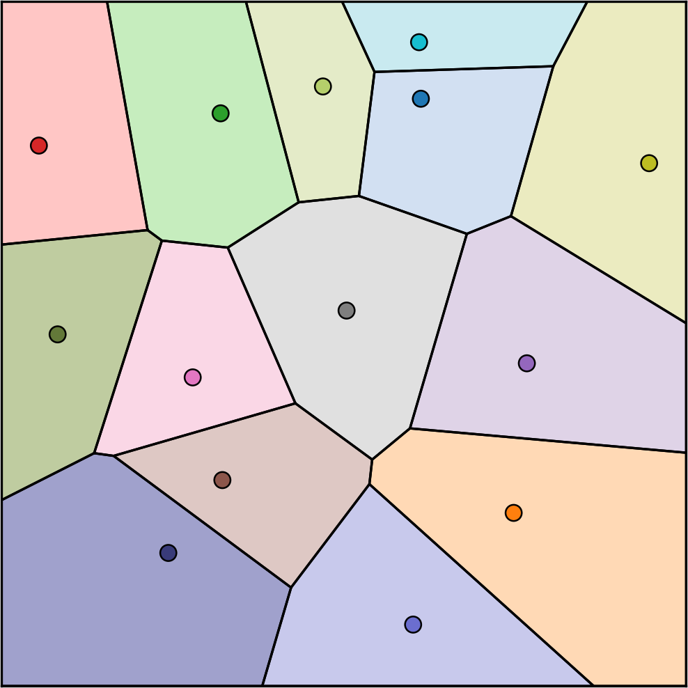
A Voronoi diagram, illustrated in Figure 3, is the first stage (Becker and Solomon, Reference Becker and Solomon2022: 321–3). Voronoi diagrams work by placing a set of points on a plane and then partitioning the plane based on the seed to which each point is closest. All areas closest to a red or blue seed, for example, are colored red or blue. These partitioned areas represent separate Voronoi cells. Voronoi cells ensure that all areas in a jurisdiction are assigned to a single contiguous district (Fifield et al., Reference Fifield, Higgins, Imai and Tarr2020: 717).Footnote 6 For our purposes, raster squares whose centroid falls within the same Voronoi cell are partitioned into the same simulated polling division. The number of seeds we use in a district is arbitrarily designed to create an average of about 4000 electors in each cell. Notably, the only spaces we allow the Voronoi seeds to occupy are the centroids of the squares created by the fractionalized raster. The probability of a seed appearing within a square is also weighted by the count of electors in that square. This approach increases the probability of seeds being positioned in areas of high population density, where more polling divisions are needed. Notably, this addresses the challenge of the severely uneven population densities in Canada.
Voronoi Cells.

The second stage is the optimization step. MaRiPoSa calculates three properties of every partition. First, it computes the variance in the count of electors between Voronoi cells, ${\sigma _{{\rm{electors}}}}$
. Second, it checks for any overlapping seeds. Finally, it checks for electoral districts whose adjacency graph has disconnected components. The optimization step minimises the objective function:
${\sigma _{{\rm{electors}}}}$
. Second, it checks for any overlapping seeds. Finally, it checks for electoral districts whose adjacency graph has disconnected components. The optimization step minimises the objective function:
 \begin{align}\min_{x} f(x) = \sigma_{\mathrm{electors}} + \mathrm{pen}_{\mathrm{geo}}\end{align}
where $\rm pe{n_{geo}} = \left\{ {\matrix{{{{10}^9},} & {if\;any\;discontiguity\;or\;overlap\;is\;present,\,} \cr \!\!\!\!\!{0,} & \!\!\!\!\!\!\!\!\!\!\!\!\!\!\!\!\!\!\!\!\!\!\!\!\!\!\!\!\!\!\!\!\!\!\!\!\!\!\!\!\!\!\!\!\!\!\!\!\!\!\!\!\!\!\!\!\!\!\!\!\!\!\!\!\!\!\!\!\!\!\!\!\!\!\!\! {otherwise.} \cr } } \right.$
The penalty factor ${10^9}$
massively inflates the value of the objective function whenever two or more seeds occupy the same location or an electoral district’s adjacency graph is disconnected.
${10^9}$
massively inflates the value of the objective function whenever two or more seeds occupy the same location or an electoral district’s adjacency graph is disconnected.
We use Simulated Dual Annealing (SDA) to minimize Equation (1). SDA is an optimization technique that combines a global search with a model exploring local areas within a solution space (Ricca and Simeone, Reference Ricca and Simeone2008: 1417; Xiang et al., Reference Xiang, Sun, Fan and Gong1997). MaRiPoSa adapts SDA by using the global search phase to situate the Voronoi seeds stochastically within the boundaries of the province. The search phase adjusts the positions of those points while recording the value of the objective function after each adjustment. When a movement of seeds within a search generates a configuration of simulated polling divisions that reduces the value of the objective function, the movement tends to be preserved, though suboptimal moves are occasionally accepted to escape from local minima. After the search phase, the positions of the seeds are once again redistributed randomly throughout the province and the process repeats. After any number of iterations, the algorithm returns the encountered seed positions that minimized the value of the objective function.
Figure 4 visualizes this process for the electoral district of Ajax, Ontario. The fractionalized raster data of the electoral district, in the top left, is converted into the adjacency graph in the top right. The adjacency graph treats each raster square as a node, with edges between nodes indicating (rook) adjacency. Each graph has one component, so it is possible to move from any square to any other square in the district by following edges between adjacent squares. The function then positions an initial set of Voronoi seeds within the boundaries of the electoral district and partitions the graph into components based on the Voronoi seed to which each node is closest. In the optimization step, represented in the center of the graph, the positions of the seeds are adjusted, the components are reconstituted, and the value of the objective function is recorded. After ten million iterations, the algorithm returns the seed positions that minimized the value of the objective function. The bottom left of the graph visualizes the optimal encountered configuration of node assignments, and the bottom right visualizes the aggregated view of the Voronoi polling divisions to which these node assignments correspond.
Simulated Voronoi Polling Divisions, Ajax, Ontario, 2021.

Figure 5 demonstrates the progress of the optimization strategy by plotting the distribution of electors across all simulated polling divisions in Ontario after one hundred evaluations, a thousand evaluations, and so on. The number of electors in a polling division is represented along the y-axis, and the 2688 divisions are ranked along the x-axis by their number of electors. Notice how the variance in the number of electors between divisions decreases with each order-of-magnitude increase in the number of evaluations (iterations). In the initial partition, there is considerable variance between polling divisions in their elector counts: some divisions have just a few hundred electors while others have nearly 8000. After adjusting the positions of the Voronoi seeds for a million evaluations, however, a high degree of equality is achieved: all polling divisions in the province are within a few hundred voters of the average (3909), and more than 50 per cent of the districts are within fewer than 100 voters of the average. In short, the optimization strategy equalizes the number of electors between divisions, which was its objective. Note, however, that computation time (indicated parenthetically in the legend) increases approximately linearly with the number of evaluations, whereas improvement in the objective score is logarithmic. This suggests diminishing returns: excellent solutions are cheap, but perfection is prohibitively costly.
Elector Variance in Ontario Voronoi Districts after Iterations, Optimized for Equality through Dual Annealing.

Fractionalized rasterization and Voronoi partitions are the beginning and intermediary steps in MaRiPoSa. These steps resolve the complexity of Canadian political geography and the uneven distribution of electors, and they constrain the tendency of fully random processes to generate fractal boundaries with unrealistic compactness (Duchin, Reference Duchin, Duchin and Walch2022: 15). However, we do not want fractionalization and Voronoi divisions themselves to affect election outcomes in electoral districts—and conceivably they could, in cases where low resolution induces tessellation errors sufficient to change the results of close races. In these cases, the resolution of the raster would need to be increased. In our study, the district of Châteauguay–Lacolle in Quebec, which the Liberals won by 12 votes, was the only district in Canada switched by a tessellation error at its boundaries. Although we could increase the raster resolution in Quebec to accommodate this district, for present purposes the additional computational cost is not justified by the marginal increase in accuracy; thus, we acknowledge and accept the imprecision.
Simulated electoral districts
The simplification of political geography allows us to represent a province and regions of a province as an adjacency graph of nodes where each node represents a Voronoi polling division instead of a raster square. This adjacency graph is the input for this stage of the analysis. As before, we use Voronoi cells to create districts and SDA to optimize the position of the Voronoi seeds. In this case, however, we do not seek only to minimize the variance in the number of electors between districts; instead, the objective function we minimize is defined by the number of seats a target party loses from a set of valid configurations of electoral district boundaries, where validity is delineated by a set of constraints.
For our purposes, allowable population variance is defined in relation to the distribution of the population observed within the actual boundaries. This implies two constraints. First, simulated districts are almost never outside the boundaries of $ \pm 25$
per cent of the average population in the districts, which is true of actual boundaries also. Second, in our strictest interpretation, the variance of population between simulated districts must be more equal than the variance between the original districts. These constraints are far more stringent than law and practice require in Canada (Barnes, Reference Barnes2024: 3; Johnson, Reference Johnson1994), and they make it more challenging for the algorithm to find configurations that benefit one party over another. In this sense, our results are conservative. Moreover, we only have population data at the level of electoral districts, which means we must estimate population counts in polling divisions based on the share of an electoral district’s electors within each polling division. Even so, we use population counts from the 2011 census rather than electors in 2021 as the constraint on inequality between simulated electoral districts. We do this for two reasons. First, Canadian boundary commissions used the 2011 population counts to create the districts in the first place, as the census estimate is the required metric in Canada. The original boundaries were clearly constrained by the
$ \pm 25$
per cent of the average population in the districts, which is true of actual boundaries also. Second, in our strictest interpretation, the variance of population between simulated districts must be more equal than the variance between the original districts. These constraints are far more stringent than law and practice require in Canada (Barnes, Reference Barnes2024: 3; Johnson, Reference Johnson1994), and they make it more challenging for the algorithm to find configurations that benefit one party over another. In this sense, our results are conservative. Moreover, we only have population data at the level of electoral districts, which means we must estimate population counts in polling divisions based on the share of an electoral district’s electors within each polling division. Even so, we use population counts from the 2011 census rather than electors in 2021 as the constraint on inequality between simulated electoral districts. We do this for two reasons. First, Canadian boundary commissions used the 2011 population counts to create the districts in the first place, as the census estimate is the required metric in Canada. The original boundaries were clearly constrained by the $ \pm 25$
per cent guideline, with few exceptions. Second, the results of our analysis are also much less pronounced when we constrain simulated districts based on the inequality of population rather than the inequality of electors. As it turns out, the decision to equalize population instead of electors is highly consequential in Canada. Here again, we err on the side of being overly conservative by constraining population inequality.
$ \pm 25$
per cent guideline, with few exceptions. Second, the results of our analysis are also much less pronounced when we constrain simulated districts based on the inequality of population rather than the inequality of electors. As it turns out, the decision to equalize population instead of electors is highly consequential in Canada. Here again, we err on the side of being overly conservative by constraining population inequality.
Finally, we impose still further constraints by processing large provinces in sub-regions (for example, “GTA West,” “Alberta South”) and constraining population variance in relation to variance observed in the original configuration in each sub-region. Although Canadian law leaves this to the discretion of boundary commissions, and although this self-imposed constraint further reduces the magnitude of our results, it does have the practical advantage of allowing users to parallelize the algorithm and distribute its processing, which significantly speeds up the computation for large provinces. In any case, other researchers can specify their own constraints and use whatever level of analysis they choose. For our purposes, what we wish to test is the algorithm’s ability to generate valid configurations that generate discrepant election outcomes. In addition to the strict condition of “less population variance” (that is, $ + 0$
), we also experiment with tolerances of an additional 5 and 10 per cent population deviation within each subregion. Although tolerances of this magnitude continue to generate configurations that are well within Canadian law, we want to test whether the additional incremental increases in tolerance for population deviations allow for greater discrepancies in potential partisan outcomes. If greater flexibility in allowable population deviations generates a greater range of outcomes, we expect this greater range of outcomes to make it easier for the algorithm to discover allowable configurations that optimize a partisan outcome of interest. Keep in mind that we are incrementally adding
$ + 0$
), we also experiment with tolerances of an additional 5 and 10 per cent population deviation within each subregion. Although tolerances of this magnitude continue to generate configurations that are well within Canadian law, we want to test whether the additional incremental increases in tolerance for population deviations allow for greater discrepancies in potential partisan outcomes. If greater flexibility in allowable population deviations generates a greater range of outcomes, we expect this greater range of outcomes to make it easier for the algorithm to discover allowable configurations that optimize a partisan outcome of interest. Keep in mind that we are incrementally adding $ + 5$
and
$ + 5$
and $ + 10$
tolerances, which are sufficient for demonstration purposes but much less than the
$ + 10$
tolerances, which are sufficient for demonstration purposes but much less than the $ + 25$
(and occasionally beyond) routinely tolerated by Canadian boundary commissions.
$ + 25$
(and occasionally beyond) routinely tolerated by Canadian boundary commissions.
For our purposes, the difference in standard deviation is: $\Delta \sigma = {\sigma _{{\rm{sim}}}} - {\sigma _{{\rm{obs}}}},$
where ${\sigma _{{\rm{sim}}}}$
is the standard deviation in population between districts in the simulated configuration, and
${\sigma _{{\rm{sim}}}}$
is the standard deviation in population between districts in the simulated configuration, and ${\sigma _{{\rm{obs}}}}$
is the standard deviation in population between districts in the actual configuration. When we allow additional tolerance
${\sigma _{{\rm{obs}}}}$
is the standard deviation in population between districts in the actual configuration. When we allow additional tolerance $\tau$
, we define the variance penalty as:
$\tau$
, we define the variance penalty as: ${\rm{pe}}{{\rm{n}}_\sigma } = \left\{ {\matrix{ \!\!\!\!\!\!\!\!\!\!\!\! \!\!{0,} & \;\;{{\rm{if}}\;\Delta \sigma \le \tau ,} \cr {\Delta \sigma - \tau ,} & {{\rm{otherwise}}.} \cr } } \right.$
Population variance is penalized if and only if the simulated configuration’s standard deviation exceeds the actual configuration’s standard deviation by more than the tolerance threshold. We apply the soft plus function— $log(1+e^{x})$
—to the variance penalty, smoothing its behaviour near zero. This mimics ReLU but avoids the sharp kink and non-differentiability at zero that disrupted optimization. By way of explanation, imagine a line graph where the value of
$log(1+e^{x})$
—to the variance penalty, smoothing its behaviour near zero. This mimics ReLU but avoids the sharp kink and non-differentiability at zero that disrupted optimization. By way of explanation, imagine a line graph where the value of $y$
is always
$y$
is always $0$
when
$0$
when $x \le 0$
, and then, when
$x \le 0$
, and then, when $x{\rm{ \gt }}0$
, the value of
$x{\rm{ \gt }}0$
, the value of $y$
equals
$y$
equals $x$
. This is a ReLU (Rectified Linear Unit) function which says, in effect: impose an increasingly large penalty as
$x$
. This is a ReLU (Rectified Linear Unit) function which says, in effect: impose an increasingly large penalty as $x{\rm{ \gt }}0$
but do not impose any penalty when
$x{\rm{ \gt }}0$
but do not impose any penalty when $x \le 0$
. Notice how this function is precisely what we want in this case, where we impose increasingly large penalties on simulated outcomes as the population variance between simulated electoral districts is larger than what we observed in the actual partition (that is,
$x \le 0$
. Notice how this function is precisely what we want in this case, where we impose increasingly large penalties on simulated outcomes as the population variance between simulated electoral districts is larger than what we observed in the actual partition (that is, $y = f\left( x \right),x{\rm{ \gt }}0$
), but we want to impose no penalty when the population variance between simulated districts is equal to, or less than, the variance in the actual partition (that is,
$y = f\left( x \right),x{\rm{ \gt }}0$
), but we want to impose no penalty when the population variance between simulated districts is equal to, or less than, the variance in the actual partition (that is, $y = 0,x \le 0$
). The gradient of the penalty allows the algorithm to “find its way” to the allowable configurations of boundaries. The problem, however, is that the algorithm struggled to find optimal configurations when we used a ReLU function, we presume because the ReLU function creates a “kink” when
$y = 0,x \le 0$
). The gradient of the penalty allows the algorithm to “find its way” to the allowable configurations of boundaries. The problem, however, is that the algorithm struggled to find optimal configurations when we used a ReLU function, we presume because the ReLU function creates a “kink” when $x = 0$
. This causes our optimization to go awry because the algorithm tended not to want to cross
$x = 0$
. This causes our optimization to go awry because the algorithm tended not to want to cross $0$
. Thus, we follow the common practice of approximating the ReLU function with a Softplus function, which smoothens the value of
$0$
. Thus, we follow the common practice of approximating the ReLU function with a Softplus function, which smoothens the value of $f\left( x \right)$
as
$f\left( x \right)$
as $x \to 0$
and is differentiable across the domain. Euler’s number,
$x \to 0$
and is differentiable across the domain. Euler’s number, $e \approx 2.718$
, appears here because it is the only number such that the derivative of the function
$e \approx 2.718$
, appears here because it is the only number such that the derivative of the function $f\left( x \right) = {e^x}$
is equal to
$f\left( x \right) = {e^x}$
is equal to ${e^x}$
at all points. This property makes it particularly useful for functions modelling growth or decay, which is why we use it in this case to model the variance penalty.
${e^x}$
at all points. This property makes it particularly useful for functions modelling growth or decay, which is why we use it in this case to model the variance penalty.
Finally, as with the construction of Voronoi polling divisions from raster squares, all Voronoi divisions within an electoral district must be fully connected in the adjacency graph. Moreover, the number of districts in the simulated configuration must be equal to the number of districts in the actual configuration. Thus, overlapping seeds are not permitted. Formally, the geometric penalty is defined as: ${\rm{pe}}{{\rm{n}}_{{\rm{geo}}}} = \left\{ {\matrix{ {{ {10}^9},} & {{\rm{if}}\;{\rm{any}}\;{\rm{discontiguity}}\;{\rm{or}}\;{\rm{overlap}}\;{\rm{is}}\;{\rm{present}},} \cr \!\!\!{0,} & \!\!\!\!\!\!\!\!\!\!\!\!\!\!\!\!\!\!\!\!\!\!\!\!\!\!\!\!\!\!\!\!\!\!\!\!\!\!\!\!\!\!\!\!\!\!\!\!\!\!\!\!\!\!\!\!\!\!\!\!\!\!\!\!\!\!\!\!\!\!\!\!\!\!\! {{\rm{otherwise}}.} \cr } } \right.$
A violation of the contiguity constraint returns a penalty score of ${10^9}$
, which precludes any such configurations from the set of valid configurations.
${10^9}$
, which precludes any such configurations from the set of valid configurations.
The target objective is the difference in wins for a target party in the simulated vs the actual configuration of electoral district boundaries. The difference in the target party’s electoral outcomes is the wins difference: ${\bf{win}}{{\bf{s}}_{{\rm{diff}}}}\; = \;{\rm{win}}{{\rm{s}}_{{\rm{obs}}}}\; - \;{\rm{win}}{{\rm{s}}_{{\rm{sim}}}},$
where, for any region:
-
• ${\rm{win}}{{\rm{s}}_{{\rm{obs}}}}$
: number of seats the target party won in the actual election,
${\rm{win}}{{\rm{s}}_{{\rm{obs}}}}$
: number of seats the target party won in the actual election, -
•
${\rm{win}}{{\rm{s}}_{{\rm{sim}}}}$
: number of seats the target party won in the simulated scenario.


As the objective function is to be minimized, a negative value of the wins difference indicates that the target party won more seats in the simulated configuration than in the actual configuration. Notably, the objective function can be tweaked to harm instead of benefit a target party, or to increase or decrease the difference between a target party’s count of seats and the count of seats won by another party. A target margin of victory can also be set, such that the objective function is minimized subject to the constraint that the target party wins by a certain margin. Other constraints, such as territorial compactness, can also be added, though, due to the computational cost involved in calculating standard measures of compactness, the process is more technically involved than simply calculating compactness of plausible iterations. As there is no compactness requirement in Canada (Taylor et al., Reference Taylor, Lucas, Kirby and Hewitt2023), and our Voronoi cells, unlike some other approaches, like single-flip continuous (DeFord et al., Reference DeFord, Duchin and Solomon2021: 4), tends to generate reasonably compact districts anyway, we record compactness but do not undertake here the technical task of developing proxy measure that are feasible to calculate in our optimization process.
Objective
In our case, the objective function $f\left( {\bf{x}} \right)$
is the sum of all penalties minus the wins difference:
$f\left( {\bf{x}} \right)$
is the sum of all penalties minus the wins difference: $\mathop {{\rm{min}}}\limits_{\bf{x}} \,f\left( {\bf{x}} \right) = {\rm{log}}\left( {1 + {e^{{\rm{pe}}{{\rm{n}}_{\rm{\sigma }}}}}} \right) + {\rm{pe}}{{\rm{n}}_{{\rm{geo}}}} - {\bf{win}}{{\bf{s}}_{{\rm{diff}}}}$
Notice that the value of $f\left( {\bf{x}} \right)$
is dominated by penalties until the penalties sum to 0, in which case the value of
$f\left( {\bf{x}} \right)$
is dominated by penalties until the penalties sum to 0, in which case the value of $f\left( {\bf{x}} \right)$
is determined by the wins difference. In effect, minimizing
$f\left( {\bf{x}} \right)$
is determined by the wins difference. In effect, minimizing $f\left( {\bf{x}} \right)$
means searching for sets of boundaries that are allowable (for example, contiguous and more equitable than, or within tolerance of, the population distribution in the observed boundaries), and only then searching, among these configurations, for boundaries that generate the greatest gain in seats for a target party.
$f\left( {\bf{x}} \right)$
means searching for sets of boundaries that are allowable (for example, contiguous and more equitable than, or within tolerance of, the population distribution in the observed boundaries), and only then searching, among these configurations, for boundaries that generate the greatest gain in seats for a target party.
Our optimization step is substantively the same as the approach discussed above for the creation of Voronoi polling divisions. As before, we use Voronoi cells to create districts and Simulated Dual Annealing to optimize the position of the Voronoi seeds. In this case, however, we use a million iterations for each locale and minimize the number of seats a target party loses from a set of valid configurations of electoral district boundaries, where “valid” is defined to ensure a legal and equitable population distribution vis-a-vis the actual partition.
Results
The Liberals finished the 2021 election with 32.6 per cent of the vote, which was 1.1 percentage points behind the Conservative party. Nonetheless, the Liberals won 160 of 338 seats, while the Conservatives won 119. The Bloc Québécois (BQ), New Democratic Party (NDP) and Greens won 32, 25 and 2 seats, respectively. The conventional understanding is that the Liberal vote was more “efficient” because it was concentrated in competitive regions of the country, whereas the Conservative vote was too concentrated in the Prairie provinces and rural areas where elections are less competitive. At best, this is only part of the story.
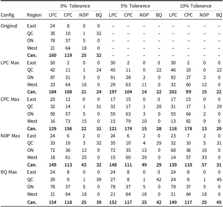
The results in Table 1 summarize the seats each party receives when votes are counted according to original and alternative configurations of district boundaries in Canadian provinces.Footnote
7
The alternative configurations, represented in the first column, are optimized for each party from among the sets of valid configurations. “LPC Max” optimizes for additional Liberal Party of Canada (LPC) seats, “CPC Max” for additional Conservative Party of Canada (CPC) seats and so on. The regions, represented in the second column, are summary categories of the processing that took place within provinces. All valid configurations are contiguous, and the table summarizes separately the results arising from three constraints on the allowable population variation between districts. These constraints are represented by the three horizonal blocks of columns in the table. The first and strictest constraint ( $ + 0$
) requires population variation to be less than or equal to the actual variation between districts in each locale, while the second and third constraints allow for additional tolerance of 5 and 10 per cent of the average population size in each locale (that is, the locale electoral quotient equivalent).
$ + 0$
) requires population variation to be less than or equal to the actual variation between districts in each locale, while the second and third constraints allow for additional tolerance of 5 and 10 per cent of the average population size in each locale (that is, the locale electoral quotient equivalent).
Original and Optimized Outcomes, with Alternative Constraints on Population Variance

Notes:
1. All simulations are carried out within provinces.
2. National totals include YT, NU, and NT (+2 LPC, +1 NDP).
3. For BQ Max, results outside Quebec are the original observed values.
4. Reported values show outcomes under a 0%, 5%, and 10% additional population-variance tolerances, relative to observed baseline. Percentage is of average observed district size in the locale (i.e., locale Electoral Quotient equivalent).
5. Green Party seats are tabulated but not shown (0–2 seats across all scenarios).
6. When the optimizer does not find an allowable configuration (objective ≥ 0), the original seat counts are used.
From this vantage point, if we look left to right across the five rows in LPC Max, which optimizes for Liberal seats, we see the seat counts for each party in each region when the pro-Liberal optimizer is constrained by population variances of $ \le + 0$
in the first block, then by
$ \le + 0$
in the first block, then by $ \le + 5$
in the second block and finally by
$ \le + 5$
in the second block and finally by $ \le + 10$
in the third. Notice that the Liberals win 42 seats in Quebec and 184 seats overall under the most stringent constraint (
$ \le + 10$
in the third. Notice that the Liberals win 42 seats in Quebec and 184 seats overall under the most stringent constraint ( $ \le + 0$
), while they win 45 and 46 seats in Quebec, and 197 and 202 seats overall, under the more relaxed constraints. Relative to the actual results, the overall seat count when districts are optimized for the Liberals represent gains of 24, 37 and 42 seats for population variance tolerances of 0, 5 and 10 percentage points, respectively. The key finding is that there are configurations of boundaries that generate a more equitable population distribution and an additional 24 seats for the Liberals, and the Liberal gains increase as the constraints on population variance are relaxed. Notably, each of these configurations turn the Liberal minority outcome into a majority government. There are corresponding losses of seats for each of the other parties.
$ \le + 0$
), while they win 45 and 46 seats in Quebec, and 197 and 202 seats overall, under the more relaxed constraints. Relative to the actual results, the overall seat count when districts are optimized for the Liberals represent gains of 24, 37 and 42 seats for population variance tolerances of 0, 5 and 10 percentage points, respectively. The key finding is that there are configurations of boundaries that generate a more equitable population distribution and an additional 24 seats for the Liberals, and the Liberal gains increase as the constraints on population variance are relaxed. Notably, each of these configurations turn the Liberal minority outcome into a majority government. There are corresponding losses of seats for each of the other parties.
When optimizing for Conservative seats, which is summarized in the CPC Max rows, there are configurations that generate more equitable population distributions and 156 seats for the Conservatives, a gain of 37 seats for the party relative to their actual performance in the election. Such an outcome would have resulted in a Conservative minority government instead of a Liberal minority government. As with the Liberals, the pro-Conservative optimizer finds more seats for the target party when the constraints on population variance are relaxed. Relaxing the population variance constraint by $5$
allows the algorithm to find a configuration that generates 174 seats for the Conservatives, which is a majority government. Relaxing the constraint by
$5$
allows the algorithm to find a configuration that generates 174 seats for the Conservatives, which is a majority government. Relaxing the constraint by $10$
uncovers 178 seats for the Conservatives, which would be a majority government of equivalent magnitude to the party’s result in the 2011 election.
$10$
uncovers 178 seats for the Conservatives, which would be a majority government of equivalent magnitude to the party’s result in the 2011 election.
For the NDP and the BQ, the optimized configurations do not affect the overall outcome of the election, but they nonetheless generate narrative changing outcomes for both parties. There are valid configurations that return at least 39 seats for the Bloc in Quebec under the strictest constraint, and up to 42 and 45 seats under the more relaxed constraints—the latter representing a result the party has not achieved since 2008. The NDP, meanwhile, was shut out of Saskatchewan, Nova Scotia and Toronto—which was a noteworthy failure for the party. As it turns out, however, there are valid and more equitable configurations in each of Saskatoon, Halifax and downtown Toronto that would have returned at least one seat in each city for the NDP. Overall, there are valid and more equitable configurations returning 43 seats for the NDP—18 more than they received in the actual election. When population variance constraints are relaxed, the algorithm finds allowable configurations returning 49 and 57 seats for the party, which would have represented the second best showing in the party’s 50-year history.
In addition to alternative outcomes, MaRiPoSa uncovers the boundaries of “latent districts” and “potential seats” for parties across locales throughout Canada. The Census Metropolitan Area of Ottawa, for example, can be either a nine-to-one Liberal stronghold or 50/50 split with the Conservatives, depending on which configuration of valid (and equally compact) districts are chosen. The Liberals won seven of ten districts in Northern Ontario, but there are configurations of districts in this same region that would return more seats to the Conservatives than the Liberals. The same pattern applies to the eastern Greater Toronto Area and other parts of the province. There is nothing special about Ontario in this respect. In New Brunswick, where the Liberals won six of ten seats, there are valid configurations returning seven of ten seats for the Conservatives or nine of ten seats for the Liberals. Similarly, the BQ won four of nine seats in the Eastern Townships of Quebec, but there are valid configurations of districts that would have returned at least seven of nine seats for the BQ. The Liberals won three seats in the region but could have won at least four; the Conservatives won two seats but could have won at least three. And so on across Canada.
At a higher level of granularity, MaRiPoSa uncovers the locales across Canada where boundaries are most consequential, as well as specific “latent potential districts” within those locales to produce seats for different parties. Figure 6, for example, shows two electoral districts in the downtown region of Saskatoon, both of which elected Conservatives in the 2021 election. Indeed, the NDP was shutout entirely from Saskatchewan. Figure 6, however, is a valid potential district in the same region as Figure 6, except with boundaries enclosing a plurality vote for the NDP by a margin of less than 1 per cent over the Conservatives. Thus, there was at least one potential district in Saskatchewan where NDP candidates received more votes than any other party. There are other potential NDP districts also. Projecting the boundaries on Google Earth or equivalent reveals that one such hypothetical NDP district, which would have a larger winning margin than the one shown in Figure 6, extends from the University of Saskatchewan in the northeast to just beyond St. Paul’s Hospital in the northwest, south to the Queen Elizabeth Power Station and then east again along Highway 11 to the interchange with the Trans-Canada. It would be trivial to develop—and to automate the development—of an argument for a potential district along these lines. Indeed, the nearly 67,000 people living within the boundaries of this potential district would be within 10 per cent of the average population size of Saskatchewan districts, which is well within the allowable limits of $ \pm 25$
per cent. The vantage point in Figure 6 is highly granular, but the result is otherwise typical. There are potential NDP districts in downtown Toronto and Halifax and in other parts of the country. There are Conservative districts in downtown Toronto. The same goes for these and other parties in other places.
$ \pm 25$
per cent. The vantage point in Figure 6 is highly granular, but the result is otherwise typical. There are potential NDP districts in downtown Toronto and Halifax and in other parts of the country. There are Conservative districts in downtown Toronto. The same goes for these and other parties in other places.
Electoral Districts and Potential Districts in Saskatoon, SK.

Conclusion
As its critics emphasize, Canada’s SMP system is designed to reward regional support at the expense of diffuse support. It also prioritizes territorially-based political interests over other kinds of interests (Cairns, Reference Cairns1968), at least for small parties (Johnston and Ballantyne, Reference Johnston and Ballantyne1977). Boundary effects, however, are distinctive phenomena. The causes of boundary effects are complex (Stevens et al., Reference Stevens, Islam, de Geus, Goldberg, McAndrews, Mierke-Zatwarnicki, Loewen and Rubenson2019). Bodet et al. (Reference Bodet, Bouchard, Thomas and Tessier2022) estimate that differences in local contexts, campaigns and candidates—including incumbency—can explain, on average, 6 to 10 per cent of a party’s vote, assuming the positions of electoral district boundaries are exogenous to considerations with partisan impact (Bodet et al., Reference Bodet, Bouchard, Thomas and Tessier2022: 166). Boundary effects depend, most obviously, on where parties choose to run candidates. But boundary effects can also arise from the rules of electoral district design and how those rules are interpreted and implemented. As urbanization intensified and the boundaries between districts became less determined by distance and geography, the effects of boundaries on outcomes almost certainly became more potent—and sometimes, perhaps, decisive. The ultimate question in this domain is whether boundary effects systematically benefit some parties and voters at the expense of others. We explore this question in a subsequent paper. For now, let us answer the central question posed at the outset of this article: without changing the votes or locations of any voters, how much can we affect election outcomes by adjusting district boundaries to alternative, yet permissible, configurations? For 2021, the answer is that we can change the party that wins the election and governs the country. Additional computing and relaxed constraints generate more severe discrepancies. In short, the outcome of the 2021 election depended not only on the levels and geographic distribution of party support. Boundaries were consequential.
Computation has fundamentally changed the context in which the design of electoral district boundaries occurs. With tools like MaRiPoSa, we suspect it will become increasingly difficult to maintain the legitimacy of Canadian democracy by relying on edicts about whether, to what extent and which “…geography, community history, community interests and minority representation…” or other “…examples of considerations that may justify departure from absolute voter parity” should influence boundary decisions (Supreme Court of Canada, 1991). Human judgement will continue to be important. Boundary commissioners will struggle, however, to articulate an understanding of “effective representation of the Canadian mosaic” clearly enough to justify specific boundary choices when the partisan consequences of those choices will be immediately accessible, and therefore also salient, to the actors involved, through computing. It is one thing to accept an election result based on the way people in different regions or provinces voted. It is another thing to accept a result based on invisible lines between neighbours. Notably, the degree to which tools like MaRiPoSa will be available to parties will vary. Parties with more resources will have a significant technical advantage over smaller parties and independents. To ensure transparency and fairness—however defined—Canada will need to constrain the discretion of judges and commissions by articulating clearer principles and scrutinizing proposed boundaries more rigorously. Computing and statistics will be critical in this process, as they have been in the United States. Tools like MaRiPoSa lay the groundwork for this scrutiny in Canada.
What does it mean for our understanding of Canadian democracy, or of its political geography (Cochrane and Perrella, Reference Cochrane and Perrella2012), that the same votes in the same places can produce altogether different governments depending on the boundaries between districts? What will it mean for the practice of Canadian politics that computing makes these differences increasingly clear to political parties? Historically, Canadians looked to the experiences of other countries when formulating policies about electoral district boundaries (Courtney, Reference Courtney2001: 38). Many of these legislative committees involved panels of experts, presenting careful policy and empirical analyses, along with leading domain expertise, about elections and electoral systems (Canada, 1985; Grenier et al., Reference Grenier, Hamelin, Angell, Lemieux, Martin and Raynauld1962). To our knowledge, Canada has not held such a meeting at the federal level since the Supreme Court’s 1991 decision overruling the Saskatchewan Court of Appeal. This is an unfortunate development.
Consider the lessons for Canada, for example, from California’s 2010 referendum to end partisan gerrymandering by adopting, in effect, the same system that Canada had used since 1964. As in Canada, the California commission would hold public hearings to inform its decision-making. Despite opposition from prominent Democrats in the state, the referendum passed with over 60 per cent support from Californians. The Democrats adapted immediately. The national campaign sent emails to local party officials whenever the commission was discussing boundaries in their region. The emails encouraged the officials “…to have allies testify to ‘community of interest’ lines that supported their maps” (Pierce and Larson, Reference Pierce and Larson2011). Concerned citizens advocated for boundaries on ostensibly non-partisan lines, but in fact many of the concerned citizens were party activists and many of the boundaries were carefully and deliberately gerrymandered behind the scenes (Pierce and Larson, Reference Pierce and Larson2011). “So convenient a thing is it to be a reasonable creature,” Ben Franklin observed in his autobiography, “since it enables one to find or make a reason for everything one has a mind to do.” When it comes to redistricting, computing will amplify this capacity a trillion-fold. Canada needs to prepare for this new reality, and adapt its institutions accordingly. Canada may wish to consider a return to multi-member districts, with the aim of reducing the sensitivity of outcomes to boundaries. At a minimum, the country should consider additional constraints on the allowed population variation between districts within provinces. When coupled with computing, vastly divergent outcomes will intensify partisan concern and involvement in the next boundary design process.
Acknowledgements
I thank Joanna Everitt (UNB), Anna Essellment (Waterloo), Louise Carbert (Dalhousie), Jamie Gillis (STU), J.P. Lewis (UNB), and the audience for their feedback at the 2024 Conference of the Atlantic Provinces’ Political Science Association. I thank Laura Stephenson (Western) for her feedback on an early iteration of this project at the Conference of the American Political Association (2022), as well as Richard Johnston (UBC) for helpful context on core components of this article at the Conference of the Canadian Political Science Association (2025). Stephen White (Carleton) provided several rounds of comments on iterations of this article. I would also like to thank Jack Lucas (Calgary), Robert Vipond (Toronto), Evelyne Brie (UdeM) and the attendees at the 2025 Toronto Political Development Workshop, as well as Eric Merkely (Toronto), Michael Donnelly (Toronto) and the research team at the University of Toronto’s Politics, Elections, and Representation Lab (PEARL). I also thank Christopher Alcantara, David Armstrong, Amanda Friesen, Matthew Lebo, Andrew Sancton, Zack Taylor, Matthew Turgeon, Sebastián Vallejo Vera and their colleagues and students in the Department of Political Science at Western University for their hospitality and feedback. Last but not least, I thank my colleagues Christopher Greenaway (UTM), J.-F. Godbout (UdeM), April Lindgren (TMU), Rohan Alexander (Toronto), Zane Schwartz (Investigative Journalism Foundation), Meghan Snider (University of Toronto/Investigative Journalism Foundation), Ashley Rostamian (UofT), Semra Sevi (UofT), and students Michael Wong (UTSC/MIT), Eli Rose (UofT), Del Coburn (UofT), Kira Jensen (UofT), and the rest of our team in the Political Accountability, Transparency, and Representation Oversight Network (PATRON) at the University of Toronto.
Financial support
This research is supported by the Social Sciences and Humanities Research Council of Canada (SSHRC) Partnership Grant 895-2025-1002.
Competing interests
The author(s) declare none.






 Open access

