


I. Introduction
The price impact of an order is the extent to which its execution moves market prices. It is a measure of market liquidity and a key part of the market microstructure literature. Empirical estimates of price impact are also important for assessing whether trading strategies derived from numerous anomalies documented in the literature are profitable net of trading costs. Examples of earlier papers that examine this issue include Chen and Velikov (Reference Chen and Velikov2023), Korajczyk and Sadka (Reference Korajczyk and Sadka2004), Novy-Marx and Velikov (Reference Novy-Marx and Velikov2016), and Patton and Weller (Reference Patton and Weller2020). Practitioners closely track the price impacts of their trades because they directly diminish the performance of their portfolios. The expected price impact is also a significant factor in a fund manager’s trading and portfolio rebalancing decisions.
This literature largely focuses on trading in the continuous market. However, closing auctions have become increasingly popular over the last few years, and they serve as an alternative mechanism for trading. For instance, Jegadeesh and Wu (Reference Jegadeesh and Wu2022) find that closing auction volume accounts for about 10% of the average daily volume (ADV) in recent years and document that closing auctions attract uninformed traders.Footnote 1 Theoretical models show that an increased presence of uninformed traders results in a smaller price impact.
The opening auction is another trading mechanism, though its trading volume is significantly smaller than that in the closing auctions. However, investors who trade relatively small quantities and large investors who split orders across multiple trading mechanisms could benefit from routing a part of their orders to the opening auction, depending on the marginal price impact.
While there is extensive literature on trading in the continuous market, relatively little research exists on trading in closing auctions. This study addresses a few key questions: i) What is the price impact of trades in closing and opening auctions versus that in the continuous market? ii) How do these impacts vary across stocks with different characteristics? iii) What are the implications for trading strategies with different turnover rates? We answer these questions and provide the first comprehensive comparison of price impacts across these trading mechanisms.
We first estimate a price impact model for closing auctions. Previously, Jegadeesh and Wu (Reference Jegadeesh and Wu2022) estimate a price impact model that specifies impact as a linear function of order size to compare the liquidity of closing auctions on the NYSE versus Nasdaq. However, we find that a model in which price impact is related to the square root of order size fits the closing auctions’ data significantly better than the linear model and therefore we use the square root model in our analyses. We also find that the linear model significantly underestimates the price impact in closing auctions. For example, the price impact estimate for a 1% ADV order with the linear model in Jegadeesh and Wu (Reference Jegadeesh and Wu2022) is 2.35 bps whereas it is 17.7 bps with the square root model. We estimate price impact as a function of stock characteristics, which we use to compute trading costs for characteristics based trading strategies. We also estimate a similar model for opening auctions.
Next, we estimate the price impact for the continuous market. Earlier papers that estimate price impact models for continuous markets include Breen, Hodrick, and Korajczyk (Reference Breen, Hodrick and Korajczyk2002), Glosten and Harris (Reference Glosten and Harris1988), and Novy-Marx and Velikov (Reference Novy-Marx and Velikov2016). The price impact in the continuous market has declined over time, possibly because of increased competition across exchanges and decimalization. Because one of our objectives is to compare the price impact in auctions versus that in the continuous market, we estimate the price impact models for the continuous market also over the same recent sample period as for auctions. We estimate a square root model for this mechanism as well because it fits the data significantly better than a linear model.
The practitioner literature (see, e.g., BARRA (1997), Frazzini, Israel, and Moskowitz (Reference Frazzini, Israel and Moskowitz2018), and Grinold and Kahn (Reference Grinold and Kahn1999)) typically models price impact as a function of the square root of order size and estimates the models using real-time trades of institutional funds. However, cost estimates based on institutional trades are not generalizable to the CRSP universe because the institutional trade samples comprised bigger and relatively more liquid stocks than the CRSP universe.Footnote 2 We estimate the price impact model for continuous markets for all U.S.-traded stocks with available data.
Institutional investors often algorithmically split their large orders and trade them in smaller lots to lower the price impact. Frazzini et al. (Reference Frazzini, Israel and Moskowitz2018) report the price impacts for such algorithmically split orders executed by a large institution. We compare the price impact in closing auctions with Frazzini et al. (Reference Frazzini, Israel and Moskowitz2018) estimates to assess their relative magnitudes. Because Frazzini et al. (Reference Frazzini, Israel and Moskowitz2018) sample comprised bigger market cap and more liquid stocks, we compare the closing auction price impacts of nonmicrocap stocks (defined as stocks with market capitalizations above the 20th percentile of NYSE-listed stocks) and find that the price impact is smaller in closing auctions.Footnote 3
Finally, we compute a benchmark for the cost of trading on anomalies. Because we consider multiple mechanisms, our estimates allow us to compute the cost if traders execute their trades in the lowest cost mechanism. We consider strategies that use various stock-specific characteristics. The low turnover strategies we consider use accounting ratios such as firm size and book-to-market ratios, which are rebalanced annually. The medium and high turnover strategies we consider are a momentum strategy and 1-month return reversals, which are rebalanced monthly.
II. Closing Auctions
The NYSE and Nasdaq determine daily closing prices for stocks listed on their respective exchanges through closing auctions. We briefly explain the closing auction procedures in both exchanges here; and more detailed descriptions can be found in Bogousslavsky and Muravyev (Reference Bogousslavsky and Muravyev2023) and Jegadeesh and Wu (Reference Jegadeesh and Wu2022).
Both exchanges open their electronic order books several hours before the markets open to accept market-on-close (MOC) and limit-on-close (LOC) orders.Footnote 4 During much of our sample period, Nasdaq accepted new MOCs or modifications to existing ones until 3:50 pm and LOCs until 3:58 pm. At 4:00 pm, Nasdaq algorithmically determines the price that maximizes the number of shares matched based on on-close orders and executes the cross at that price, known as the Nasdaq Official Close Price (NOCP).Footnote 5 When there is an excess demand from LOCs at the NOCP price, Nasdaq uses time priority to allocate shares.
Similarly, the NYSE accepted new MOCs or modifications to existing ones through its electronic order book until 3:50 pm and LOCs until 3:58 pm. Floor traders at the NYSE are allowed to place or modify discretionary client orders until 3:59:50 pm.Footnote 6 The NYSE’s designated market makers (DMM) manage its closing auctions for their assigned stocks and are tasked with setting closing prices “at a level that satisfies all interest that is willing to participate at a price better than the closing auction price” (see https://www.nyse.com/article/nyse-closing-auction-insiders-guide). When there is an excess demand from LOC orders at the closing price, the NYSE uses a parity/priority rule that allows DMMs to override time priority in making allocation decisions.
A. Data and the Sample
The exchanges start disseminating closing auction data to their subscribers at the same time that they close the electronic order book and continually update the data. These data include order imbalances for each stock. The NYSE defines order imbalances as “the volume of better-priced buy (sell) shares that cannot be paired with both at-priced and better-priced sell (buy) shares at the NYSE Last Sale [price].”Footnote 7 The Nasdaq closing auction data also include similar imbalance information for Nasdaq-listed stocks.
We obtain auction data from the NYSE and Nasdaq for stocks listed on their exchanges. The data source for the NYSE is https://www.nyse.com/market-data/historical/taq-order-imbalances and for Nasdaq is https://www.nasdaq.com/solutions/data/equities/nasdaq-totalview. Our sample comprised common stocks, share codes = 10 or 11 on CRSP. We exclude other securities such as preferred shares, American Depositary Receipts, closed end funds, warrants, and REITs because one of our objectives is to compute the execution costs to trade based on anomalies and most of the anomalies are based on samples of common stocks. Our sample period is from January 2012 to December 2021. Because one of our goals is to compare the price impacts in auctions versus those in continuous markets, our sample comprised the intersection of stocks in the auction data set and the intraday microseconds Trade and Quote (TAQ) data, which we use for the continuous market.
Table 1 reports the summary statistics for all CRSP stocks, CRSP stocks listed on the NYSE and Nasdaq, and the stocks in the intersection of TAQ and auction data sets. During our sample period, the average number of NYSE/Nasdaq stocks in CRSP is 3,523 and the TAQ/Auctions sample is 2,980, which accounts for 95.6% of the market capitalization of all CRSP stocks. Looking at the size decile rank (with breakpoints constructed from the full sample of NYSE stocks), the TAQ/Auctions stocks are slightly bigger (average decile rank of 4.21 for TAQ/Auctions vs. 3.79 for CRSP stocks; average market capitalization of $1,080 million for TAQ/Auctions vs. $751 million for CRSP stocks). TAQ/Auctions stocks are also slightly more liquid (measured by trading volume) than all stocks.

B. Closing Auction Volume
Graph A of Figure 1 plots the rolling 180-day moving average of the total closing auction volume as a percentage of ADV from 2012 to 2021. The X-axis is the ending date of each 180-day window and the Y-axis is the cross-sectional average of the daily closing auction volume as a percentage of ADV. The closing auction volume steadily grows from about 4% ADV at the beginning of the sample period to a peak of about 10% ADV at the end. Table 2 presents summary statistics for the closing auction trading volume. The average trading volume during our sample period is 7.10% ADV and the median is 5.34% ADV. The trading volume distribution is positively skewed and the difference between the median and the 90th percentile is about twice that between the median and the 10th percentile.
Figure 1 plots the closing auction volume over time. Graph A represents the 180-day moving averages of the closing auction volume as a percentage of ADV, while Graph B presents the daily cross-sectional mean of closing auction volumes as a percentage of ADV. The sample comprised all NYSE and Nasdaq stocks that have data on TAQ, and the auctions data provided by the NYSE and Nasdaq. The sample period is from January 2012 to December 2021.


Graph B of Figure 1 also plots the cross-sectional median of daily closing auction volume, which shows significant spikes on Fridays. Bogousslavsky and Muravyev (Reference Bogousslavsky and Muravyev2023) attribute the spikes to the fact that options expire on Fridays. The Friday spikes are bigger on triple-witching days, when future contracts, equity index options, and options on individual stocks all expire.
Table 2 presents the summary statistics for the closing auction volume. We report the closing auction volume as a percentage of the ADV over the previous 10 days. We calculate the cross-sectional statistics (means, median, standard deviation, 10th, and 90th percentiles) daily and report their time-series averages. The table reports the statistics for all stocks, as well as partitioned subsamples based on market capitalization. The “Large” category comprised all stocks with market capitalizations greater than the median NYSE market capitalization and the “Small” category comprised all stocks with market capitalizations between the 20th and the 50th percentile of the market capitalizations of the NYSE stocks. The “Micro” category comprised all stocks with market capitalizations less than the 20th percentile of all NYSE stocks.
The closing auction trading volumes for Large and Small stocks are bigger than those for Micro stocks. Jegadeesh and Wu (Reference Jegadeesh and Wu2022) find that stocks in the indices tracked by ETFs are more actively traded in closing auctions and Micro stocks are less likely to be held in these ETFs. The average Friday volume is bigger than that for all days for all size categories.
Table 2 also reports closing auction trading volumes on earnings announcement days (EADs), which we define as days when earnings are announced after close. Because trading volume distribution is highly skewed, we compute the statistics for EADs in the table using only days when there are at least 62 stocks in the sample, which is the 25th percentile of the distribution of the number of EAD stocks per day. The average volume on EADs is 6.79% ADV, smaller than the 7.10% ADV that we observe for all days.
Overall, the closing auction volume has grown significantly over the last decade for all stocks including the Micro stocks. The closing auction volume is on average bigger on Fridays and smaller on EADs than on other days.
C. Price Impact: Closing Auctions
The auction mechanism captures the essence of the Grossman and Miller (Reference Grossman and Miller1988) model where there are two groups of participants—market makers and liquidity traders. Liquidity traders submit buy and sell orders to meet their exogenous liquidity needs, which market makers then aggregate and execute at a single clearing price. The market clearing price is above the fundamental value if the order imbalance is positive and vice versa. The resulting price impact—defined as the difference between the clearing price and the fundamental value—represents the cost liquidity traders pay for the liquidity provided by market makers.Footnote 8
There is a key difference between the closing auction settlement procedure and the determination of the market-clearing price in Grossman and Miller (Reference Grossman and Miller1988). In their model, order imbalances and market clearing prices are determined simultaneously. In contrast, in closing auctions, the time when exchanges close the electronic order books for MOC orders varied from 3:45 pm to 3:55 pm during our sample period, while the closing price is determined at 4:00 pm. The first dissemination of order imbalances coincided with the closing of MOC order books.
Jegadeesh and Wu ((Reference Jegadeesh and Wu2022), Figure 2) present the trajectory of order imbalances from the time of first dissemination to close. They show that the order imbalance is at the highest level at the time of first dissemination and then steadily declines. At the close, the order imbalances are cleared on Nasdaq, and a relatively small imbalance remains in the NYSE. The designated market maker for each stock is responsible for finding counterparties or becoming the counterparty to clear the market at the close.
1. The Model
Because one of our objectives is to compare costs under competing trading mechanisms, we focus on the expected execution cost under each one. This section estimates price impact as a function of order imbalance for closing auctions.
In closing auctions, only MOC orders are guaranteed execution and hence we consider the execution cost for traders who place such MOC orders before the exchanges close their electronic order books. We compute the order imbalance (OI) at the time of the first dissemination of closing order imbalance as
 $$ {OI}_{id}={Buy}_{id}-{Sell}_{id}, $$
where $ {Buy}_{id} $
and
$ {Buy}_{id} $
and $ {Sell}_{id} $
are the aggregate orders on the corresponding sides for stock
$ {Sell}_{id} $
are the aggregate orders on the corresponding sides for stock $ i $
on day
$ i $
on day $ d $
.
$ d $
.
Although the closing auction clears at 4:00 pm after the end of continuous market trading, the information about order imbalances OI is continually disseminated before that time. A natural question that arises is, should we compute price impact based on the price at close or at some point in time between the first OI announcement and closes? To help address this question, we start by examining the trajectory of price impact during the auction period.
The time of first dissemination of order imbalances (OIAnn) varied during our sample period as follows: i) Jan. 1, 2012 to Oct. 28, 2018–3:50 pm in Nasdaq and 3:45 pm in the NYSE, ii) Oct. 29, 2018 to Apr. 14, 2019–3:55 pm in Nasdaq; and Oct. 29, 2018 to Mar. 31, 2019–3:45 pm in NYSE, and iii) Apr. 15 to Dec. 31, 2021–3:50 pm in Nasdaq; Apr. 1, 2019 to Dec. 31, 2021–3:50 pm for NYSE. We compute price impact over multiple intervals starting from the last continuous market price before OIAnn to i) every minute after OIAnn until the last continuous market trade (“LastTrade”), and ii) at the close (“Close”). We compute realized impact at the end of interval $ \tau $
as
$ \tau $
as
 $$ {\displaystyle \begin{array}{c}{Impact}_{id}^{\tau }=\frac{P_{id}^{\tau }-{P}_{id}^{CI}}{P_{id}^{CI}},\end{array}} $$
where $ {P}_{id}^{CI} $
is the last continuous market price before OIAnn and the
$ {P}_{id}^{CI} $
is the last continuous market price before OIAnn and the $ {P}_{id}^{\tau } $
is the last price at the end of interval
$ {P}_{id}^{\tau } $
is the last price at the end of interval $ \tau $
for stock
$ \tau $
for stock $ i $
on day
$ i $
on day $ d $
.
$ d $
.
We estimate the following square root model, which specifies a relation between $ Impact $
and square root of OI normalized by ADVFootnote
9:
$ Impact $
and square root of OI normalized by ADVFootnote
9:
 $$ {\displaystyle \begin{array}{c}\mathbf{Square}\ \mathbf{root}\ \mathbf{model}:{Impact}_{id}^{\tau }={a}_{it}^{\tau }+{\lambda}_{it}^{\tau}\;\mathit{\operatorname{sign}}\left({X}_{id}\right)\sqrt{\left|{X}_{id}\right|}+{\varepsilon}_{id}^{\tau },\end{array}} $$
where $ {X}_{id}=O{I}_{id}/ AD{V}_{id} $
,
$ {X}_{id}=O{I}_{id}/ AD{V}_{id} $
, $ O{I}_{id} $
is the signed order imbalance of stock
$ O{I}_{id} $
is the signed order imbalance of stock $ i $
on day
$ i $
on day $ d $
, and
$ d $
, and $ AD{V}_{id} $
is the average trading volume of stock
$ AD{V}_{id} $
is the average trading volume of stock $ i $
over the prior 10 days. We normalize OI by ADV for comparability across stocks. We first estimate
$ i $
over the prior 10 days. We normalize OI by ADV for comparability across stocks. We first estimate $ {\lambda}_{it}^{\tau } $
for each
$ {\lambda}_{it}^{\tau } $
for each $ \tau $
within each stock month using all days
$ \tau $
within each stock month using all days $ d $
in month
$ d $
in month $ t $
.
$ t $
.
In the next stage, we fit the following cross-sectional regression each month to estimate the trajectory of $ \lambda $
from OIAnn to Close for each size category:
$ \lambda $
from OIAnn to Close for each size category:
 $$ {\displaystyle \begin{array}{c}{\lambda}_{it}^{\tau }={\theta}_{0t}^{\tau }+{\theta}_{1t}^{\tau}\;{\mathrm{NASD}}_{it-1}+{e}_t^{\tau },\end{array}} $$
where NASD is an indicator variable equal to 1 if the stock is listed on Nasdaq and zero otherwise. We add this variable because Nasdaq and the NYSE do not always start reporting OI at the same time. We also interact both the intercept and the $ \mathrm{NASD} $
indicator variable with three size categories defined earlier to account for potential differences across size categories.Footnote
10 We fit the Fama and MacBeth (Reference Fama and MacBeth1973) cross-sectional regression (4) each month with all the stocks in the sample that month.
$ \mathrm{NASD} $
indicator variable with three size categories defined earlier to account for potential differences across size categories.Footnote
10 We fit the Fama and MacBeth (Reference Fama and MacBeth1973) cross-sectional regression (4) each month with all the stocks in the sample that month.
Figure 2 presents $ {\theta}_0^{\tau} $
and
$ {\theta}_0^{\tau} $
and $ \left({\theta}_0^{\tau }+{\theta}_1^{\tau}\times \mathrm{NASD}\right) $
as functions of
$ \left({\theta}_0^{\tau }+{\theta}_1^{\tau}\times \mathrm{NASD}\right) $
as functions of $ \tau $
during the three subperiods with different times for OIAnn. As mentioned earlier, during the first subperiod, OIAnn was 3:45 pm for the NYSE and 3:50 pm for Nasdaq. We observe the following patterns:
$ \tau $
during the three subperiods with different times for OIAnn. As mentioned earlier, during the first subperiod, OIAnn was 3:45 pm for the NYSE and 3:50 pm for Nasdaq. We observe the following patterns:
-
i) $ {\theta}_0 $
exhibits significant jumps at 3:46 pm for all three size categories.
$ {\theta}_0 $
exhibits significant jumps at 3:46 pm for all three size categories. -
ii)
$ \left({\theta}_0^{\tau }+{\theta}_1^{\tau}\times \mathrm{NASD}\right) $
for each size category is the estimate of Nasdaq-listed stocks’ response in that category. The sign of these estimates fluctuates between 3:45 pm and 3:50 pm and their magnitude is small relative to
$ {\theta}_0^{\tau } $
. The estimates are all significant starting from 3:46 pm. -
iii)
$ {\theta}_0 $
in all size categories increases on average from 3:45 pm to 4:00 pm (LastTrade). -
iv) There is a sharp jump in impact from the LastTrade price close for Micro and Small stocks both in the NYSE and Nasdaq.


In Figure 2, for each stock $ i $
on day
$ i $
on day $ d $
, we compute realized impact at the end of interval
$ d $
, we compute realized impact at the end of interval $ \tau $
as
$ \tau $
as
 $$ {\displaystyle \begin{array}{c}{Impact}_{id}^{\tau }=\frac{P_{id}^{\tau }-{P}_{id}^{CI}}{P_{id}^{CI}},\end{array}} $$
where $ {P}_{id}^{CI} $
and
$ {P}_{id}^{CI} $
and $ {P}_{id}^{\tau } $
are the last continuous market price before first dissemination of order imbalances (OIAnn) and the last price at the end of the interval
$ {P}_{id}^{\tau } $
are the last continuous market price before first dissemination of order imbalances (OIAnn) and the last price at the end of the interval $ \tau $
. The last interval
$ \tau $
. The last interval $ \tau $
corresponding to 4:00 pm is denoted at 4:00 LT. We also compute price impact from the last continuous market price before OIAnn to the close (denoted as 4:00 C). We then estimate the following square root model:
$ \tau $
corresponding to 4:00 pm is denoted at 4:00 LT. We also compute price impact from the last continuous market price before OIAnn to the close (denoted as 4:00 C). We then estimate the following square root model:
 $$ {\displaystyle \begin{array}{c}{Impact}_{id}^{\tau }={a}_{it}^{\tau }+{\lambda}_{it}^{\tau}\;\mathit{\operatorname{sign}}\left({X}_{id}\right)\sqrt{\left|{X}_{id}\right|}+{\varepsilon}_{id}^{\tau },\end{array}} $$
where $ {X}_{id}=O{I}_{id}/ AD{V}_{id} $
,
$ {X}_{id}=O{I}_{id}/ AD{V}_{id} $
, $ O{I}_{id} $
is the signed order imbalance of stock
$ O{I}_{id} $
is the signed order imbalance of stock $ i $
on day
$ i $
on day $ d $
, and
$ d $
, and $ AD{V}_{id} $
is the average trading volume of stock
$ AD{V}_{id} $
is the average trading volume of stock $ i $
over 10 days prior to day
$ i $
over 10 days prior to day $ d $
. Finally, we fit the following cross-sectional regression each month to estimate the trajectory of
$ d $
. Finally, we fit the following cross-sectional regression each month to estimate the trajectory of $ \lambda $
from OIAnn to Close for each size category:
$ \lambda $
from OIAnn to Close for each size category:
 $$ {\displaystyle \begin{array}{c}{\lambda}_{it}^{\tau }={\theta}_{0t}^{\tau }+{\theta}_{1t}^{\tau}\;{\mathrm{NASD}}_{it-1}+{e}_t^{\tau },\end{array}} $$
where NASD is an indicator variable equal to 1 if the stock is listed on Nasdaq and zero otherwise. We also interact both the intercept and the NASD indicator variable with three size categories Large, Small, and Micro stocks, respectively. We classify stocks with market capitalizations above the median NYSE market capitalization as “Large,” stocks with market capitalizations between the 20th and the 50th percentile of NYSE market capitalization as “Small,” and stocks with market capitalizations smaller than the 20th percentile of NYSE market capitalization as “Micro.” The sample comprised all NYSE and Nasdaq stocks that have data on TAQ and the auctions data provided by the NYSE and Nasdaq. The time of first dissemination of order imbalances (OIAnn) is listed in the heading of each graph. The sample period is from January 2012 to December 2021.

We find similar patterns in the other subperiods as well. Observations i) and ii) indicate that OI information leads to stock price movement. Observation iii) indicates that there is some delay in stock price reaction to OI information both in the NYSE and Nasdaq, and the speed of reaction is faster for bigger stocks. The literature documents delayed reactions to intraday announcements in other contexts as well, which indicates we need to expand the observation window after OI announcements to capture the events’ full impact.Footnote 11
Observation iv) is consistent with the price jump between LastTrade and Close that Bogousslavsky and Muravyev (Reference Bogousslavsky and Muravyev2023) document. Bogousslavsky and Muravyev (Reference Bogousslavsky and Muravyev2023) also find that this price jump reverses by open the next day and hence it would be difficult for arbitrageurs to profit solely from this pattern.
At this stage, it is important to note that MOC orders are filled at the Close price and not at any intermediate prices. Therefore, in all subsequent analyses we compute price impact as
 $$ {\displaystyle \begin{array}{c}{Impact}_{id}=\frac{P_{id}^{Close}-{P}_{id}^{CI}}{P_{id}^{CI}},\end{array}} $$
where $ {P}^{Close} $
is the price at close and
$ {P}^{Close} $
is the price at close and $ {P}^{CI} $
is the last continuous market price before the NYSE first reports order imbalances.Footnote
12 We use this time for both the NYSE and Nasdaq, though Nasdaq started reporting OI a few minutes after the NYSE during much of our sample period. We use the NYSE first reporting time to account for possible information spillovers from the NYSE OI information to Nasdaq stocks.Footnote
13
$ {P}^{CI} $
is the last continuous market price before the NYSE first reports order imbalances.Footnote
12 We use this time for both the NYSE and Nasdaq, though Nasdaq started reporting OI a few minutes after the NYSE during much of our sample period. We use the NYSE first reporting time to account for possible information spillovers from the NYSE OI information to Nasdaq stocks.Footnote
13
2. Estimates
The last subsection considers a square root price impact model, but the literature also uses linear price impact models (see, e.g. Jegadeesh and Wu (Reference Jegadeesh and Wu2022), Korajczyk and Sadka (Reference Korajczyk and Sadka2004), and Novy-Marx and Velikov (Reference Novy-Marx and Velikov2016)). We now consider the following linear model and compare its performance versus the square root model:Footnote 14
 $$ {\displaystyle \begin{array}{c}\mathbf{Linear}\ \mathbf{model}: Impac{t}_{id}={a}_{it}+{\lambda}_{it}{X}_{id}+{\epsilon}_{id}.\end{array}} $$
We use the same approach as with the square root model to estimate $ {\lambda}_{it} $
for each stock month.
$ {\lambda}_{it} $
for each stock month.
Figure 3 compares fitted values from the square root and linear models with the actual average price impact for 100 categories ranked by order imbalances. For both Large and Small stocks, the square root model fitted values closely track the actual price impact for order imbalances smaller than about 5% ADV, which covers most of the observations. The linear model significantly underestimates the price impact over this range.Footnote 15 Therefore, we use the square root model from this point forward. Table A1 presents summary statistics on these price impact coefficients from the square root model. The mean price impact for 1% ADV is 17.7 bps, but the median is significantly smaller, at 8.4 bps. There is substantial heterogeneity in these price impact measures with a cross-sectional standard deviation of 34.6 bps.
Figure 3 plots the price impact for trade sizes that vary from −8% ADV to +8% ADV over the last 10 days. We present these costs for trading during closing auctions. Each day, we divide the sample into 100 groups based on the trade size. We calculate the average market impact for each of these groups. These statistics are then averaged across days, and the black dots present the actual market impact. The orange line represents the implied market impact from a square root model, while the blue line represents the implied market impact from a linear model. In the second stage, we run Fama–MacBeth regressions of market impact on lagged characteristics as those in model A of Table 3. Using estimates from those regressions, different graphs present separate cost estimates for Large, Small, and Micro stocks and for NYSE and Nasdaq stocks. We classify stocks with market capitalizations above the median NYSE market capitalization as “Large,” stocks with market capitalizations between the 20th and the 50th percentile of NYSE market capitalization as “Small,” and stocks with market capitalizations smaller than the 20th percentile of NYSE market capitalization as “Micro.” The sample comprised all NYSE and Nasdaq stocks that have data on TAQ and the auctions data provided by the NYSE and Nasdaq. The sample period is from January 2012 to December 2021.

We also examine the relation between $ \lambda $
s and additional stock-specific characteristics, which we choose based on the underlying intuition from various models. In Grossman and Miller (Reference Grossman and Miller1988), the price impact increases with the inventory risk borne by the market makers, and we use stock return volatility to proxy for this risk. The literature finds that price impact is inversely related to price, and hence, we use the log of price to capture this effect. To account for the differences between the market structures, we include an indicator variable for Nasdaq. Kyle (Reference Kyle1985) implies that price impact increases with the likelihood of informed trades, which is potentially correlated with market capitalization. Therefore, we allow the price impact to vary across size categories.
$ \lambda $
s and additional stock-specific characteristics, which we choose based on the underlying intuition from various models. In Grossman and Miller (Reference Grossman and Miller1988), the price impact increases with the inventory risk borne by the market makers, and we use stock return volatility to proxy for this risk. The literature finds that price impact is inversely related to price, and hence, we use the log of price to capture this effect. To account for the differences between the market structures, we include an indicator variable for Nasdaq. Kyle (Reference Kyle1985) implies that price impact increases with the likelihood of informed trades, which is potentially correlated with market capitalization. Therefore, we allow the price impact to vary across size categories.
We estimate the relation between the $ \lambda $
s and the additional stock characteristics using the following cross-sectional regression:
$ \lambda $
s and the additional stock characteristics using the following cross-sectional regression:
 $$ {\displaystyle \begin{array}{c}{\lambda}_{it}={\theta}_{0t}+{\theta}_{1t}{\mathrm{NASD}}_{it-1}+{\theta}_{2t}{\mathrm{Sigma}}_{it-1}-{\theta}_{3t}\mathrm{Ln}\left({\mathrm{Price}}_{it-1}\right)+{e}_{it},\end{array}} $$
where NASD is an indicator variable equal to 1 if the stock is listed on Nasdaq and zero otherwise, $ \mathrm{S}\mathrm{i}\mathrm{g}\mathrm{m}\mathrm{a} $
is the standard deviation of daily returns computed over the previous 22 days, and
$ \mathrm{l}\mathrm{n}(\mathrm{P}\mathrm{r}\mathrm{i}\mathrm{c}\mathrm{e}) $
is the natural logarithm of closing price over the previous day, adjusted for any stock splits. To account for the differences across different size categories, we interact the intercept,
$ \mathrm{S}\mathrm{i}\mathrm{g}\mathrm{m}\mathrm{a} $
is the standard deviation of daily returns computed over the previous 22 days, and
$ \mathrm{l}\mathrm{n}(\mathrm{P}\mathrm{r}\mathrm{i}\mathrm{c}\mathrm{e}) $
is the natural logarithm of closing price over the previous day, adjusted for any stock splits. To account for the differences across different size categories, we interact the intercept, $ {\theta}_0 $
, and all conditioning variables with size categories, as defined earlier. We fit the cross-sectional regression (7) each month with all the stocks in the sample that month. We use the Fama and MacBeth (Reference Fama and MacBeth1973) approach to compute the coefficient estimates and we compute their standard errors with Newey–West correction using 12 lags.
$ {\theta}_0 $
, and all conditioning variables with size categories, as defined earlier. We fit the cross-sectional regression (7) each month with all the stocks in the sample that month. We use the Fama and MacBeth (Reference Fama and MacBeth1973) approach to compute the coefficient estimates and we compute their standard errors with Newey–West correction using 12 lags.
Table 3 reports the regression estimates of equation (7) using the square root model $ \lambda $
estimates. The coefficient
$ \lambda $
estimates. The coefficient $ {\theta}_0 $
in model A for the NYSE Micro stocks is 1.82. The coefficients
$ {\theta}_0 $
in model A for the NYSE Micro stocks is 1.82. The coefficients $ {\theta}_0 $
interacted with Small and Large are significantly smaller, indicating that the price impacts are smaller for bigger stocks even with trade sizes normalized by ADV. The NASD indicator variable slope coefficients are reliably greater than zero for all three size categories, indicating that the price impact in Nasdaq is significantly bigger for all size categories. The price impacts for a 1% ADV trade implied by these estimates are 18.2, 7.4, and 4.5 bps in NYSE, and 44.7, 12.5, and 10.2 bps in Nasdaq, for Micro, Small, and Large stocks, respectively.
$ {\theta}_0 $
interacted with Small and Large are significantly smaller, indicating that the price impacts are smaller for bigger stocks even with trade sizes normalized by ADV. The NASD indicator variable slope coefficients are reliably greater than zero for all three size categories, indicating that the price impact in Nasdaq is significantly bigger for all size categories. The price impacts for a 1% ADV trade implied by these estimates are 18.2, 7.4, and 4.5 bps in NYSE, and 44.7, 12.5, and 10.2 bps in Nasdaq, for Micro, Small, and Large stocks, respectively.

Model B adds Sigma and model C further adds −ln(Price). Nasdaq stocks are, on average, more volatile and lower priced than NYSE stocks and model C controls for these differences. The NASD coefficients are statistically significantly positive for all size categories even after adding these controls. The coefficient on Sigma is significantly positive for all size categories. However, the impact of −ln(Price) on price impact is statistically significant only for Micro and Small stocks.
Jegadeesh and Wu (Reference Jegadeesh and Wu2022) use a linear model for closing auctions similar to equation (6) and estimate the model using the Fama–MacBeth approach with monthly cross-sectional regressions. Their estimated price impact is an average of 2.35 bps for all stocks, compared to our estimate of 17.7 bps. Their lower estimate is partly due to their use of a linear price impact model and partly because they employ cross-sectional regressions, whereas we use a time-series model.Footnote 16 Even our price impact estimate for large stocks is significantly larger than the estimates from Jegadeesh and Wu’s (Reference Jegadeesh and Wu2022) linear model for all stocks.
III. Price Impact: Opening Auctions
Both the NYSE and Nasdaq use opening auctions to determine open prices for stocks that have crossing interests from traders.Footnote 17 The exchanges open their order books for market-on-open and limit-on-open orders at the same time as they do for closing auctions. Nasdaq on-open orders may be entered or modified until 9:30 am and the NYSE accepts on-open orders until the stock is opened by the DMM, even if the opening is delayed beyond 9:30 am.Footnote 18 Nasdaq algorithmically determines the opening price based on the crossing interest and it constrains the price to be within a range of 10% of the best bid and ask price quotes at that time. The NYSE also determines the opening prices algorithmically if it falls within the 10% band around the reference price but if it falls outside this band, the DMM manually sets the opening price.
A. Opening Auction Volume
The auction data sets that we obtain from the NYSE and Nasdaq also contain similar details for opening auctions as those for closing auctions. Figure 4 plots the 180-day moving average of opening auction volume as a percentage ADV from 2012 to 2021. The volume reaches a peak of about 2.2% ADV in 2013 and then decreases to less than 1.5% ADV after 2015. The current opening auction volume is about 5%–10% of the closing auction volume. The mean volume spikes on Fridays and the spike is particularly large on triple-witching days. Barclay, Hendershott, and Jones (Reference Barclay, Hendershott and Jones2008) find that the surge in volume on triple-witching days is due to arbitrage activities related to index futures and options, which are settled based on the opening prices of constituent stocks.
Figure 4 plots the opening auction volume over time. Graph A presents the 180-day moving average measure for the opening auction volumes as a percentage of ADV over the last 10 days, while Graph B presents the daily cross-sectional mean of opening auction volumes as a percentage of ADV. The sample comprised all NYSE and Nasdaq stocks that have data on TAQ and the auctions data provided by the NYSE and Nasdaq. The sample period is from January 2012 to December 2021.

Table 4 presents the opening auction volume summary statistics. Overall, the average trading volume is the largest for Micro stocks at 1.76% ADV and is the smallest for Large stocks at 1.36% ADV. The average volume for all stocks on Fridays is 2.94% ADV, which is twice as large as that for all days. The volume doubles for virtually all subsamples and it is the biggest for Micro stocks. The average volume is 1.54% ADV on EADs, which is marginally lower than that on an average day.Footnote 19 Also, the median opening auction volume is 0.92% ADV, which indicates traders who seek to trade larger quantities may not find adequate liquidity in this market.

B. Opening Auctions Price Impact Estimates
This subsection estimates the square root price impact model for opening auctions. We use the opening auction data that the NYSE and Nasdaq disseminate in real time for this regression. The NYSE starts disseminating the opening information at 8:00 am and continually updates it until the stock opens for continuous trade. Nasdaq started disseminating opening information at 9:28 am from Jan. 2012 to Apr. 26, 2021, and at 9:25 am from Apr. 27, 2021 to Dec. 2021, the end of our sample period. Under both regimes, however, Nasdaq closed its MOO order book at 9:28 am. Therefore, we measure the price impact for MOO orders as
 $$ {\displaystyle \begin{array}{c} Impac{t}_{id}=\frac{P_{id}^{open}-{P}_{id}^{9:28}}{P_{id}^{9:28}},\end{array}} $$
where $ {P}^{open} $
is the open price and
$ {P}^{open} $
is the open price and $ {P}^{9:28} $
is the last premarket trade price between 9:27 am and 9:28 am on TAQ. Although the NYSE starts reporting the opening market information earlier, we measure price impact based on the order imbalances and prices as of 9:28 am to estimate the price impact model for the NYSE-listed stocks as well because premarket trades typically accumulate around that time. Intuitively, equation (8) represents the price impact for orders placed when the MOO order book is last open for both the NYSE- and Nasdaq-listed stocks.
$ {P}^{9:28} $
is the last premarket trade price between 9:27 am and 9:28 am on TAQ. Although the NYSE starts reporting the opening market information earlier, we measure price impact based on the order imbalances and prices as of 9:28 am to estimate the price impact model for the NYSE-listed stocks as well because premarket trades typically accumulate around that time. Intuitively, equation (8) represents the price impact for orders placed when the MOO order book is last open for both the NYSE- and Nasdaq-listed stocks.
Figure 5 compares fitted values from the square root and linear models with the actual average price impact for 100 categories ranked based on order imbalances as of 9:28 am. As with closing auctions, the square root model fits the data significantly better than the linear model. The figures also show that order imbalances are rarely greater than 1% ADV for Large stocks and 2% ADV for Small and Micro stocks. Therefore, the price impacts for trades outside this range should be interpreted with caution. The linear model significantly underestimates price impact within these intervals.
Figure 5 plots the price impact for trade sizes that vary from −2% ADV to +2% ADV over the last 10 days. We present these costs for trading during opening auctions. Each day, we divide the sample into 100 groups based on the trade size. We calculate the average market impact for each of these groups. These statistics are then averaged across days, and the black dots present the actual market impact. The orange line represents the implied market impact from a square root model, while the blue line represents the implied market impact from a linear model. In the second stage, we run Fama–MacBeth regressions of market impact on lagged characteristics as those in model A of Table 5. Using estimates from those regressions, different graphs present separate cost estimates for Large, Small, and Micro stocks and for NYSE and Nasdaq stocks. Large is equal to one if the stock is Large (market capitalization above the median NYSE market capitalization). We classify stocks with market capitalizations above the median NYSE market capitalization as “Large,” stocks with market capitalizations between the 20th and the 50th percentile of NYSE market capitalization as “Small,” and stocks with market capitalizations smaller than the 20th percentile of NYSE market capitalization as “Micro.” The left side of each panel plots the results for NYSE stocks, while the right side of each panel plots the results for Nasdaq stocks. The sample comprised all NYSE and Nasdaq stocks that have data on TAQ and the auctions data provided by the NYSE and Nasdaq. The sample period is from January 2012 to December 2021.

Premarket trade prices are available for only 32.8% of the stocks in our sample and we use all stocks with 9:28 am premarket prices to estimate the square root price impact model from equation (3). Table 5 presents the results of the second-stage Fama–MacBeth regression from equation (7). The slope coefficient $ {\theta}_0 $
in model A for Micro stocks is 3.34, which is significantly greater than the corresponding slope coefficient for closing auctions. The slope coefficients are also significantly bigger for Small and Large stocks. The slope coefficients on NASD and Sigma are significantly positive for all size categories in model B. However, in model C, the impact of Sigma is negative, albeit statistically insignificantly different from zero, for Micro stocks; and the impact of −ln(Price) on price impact is not statistically significant for any size category.
$ {\theta}_0 $
in model A for Micro stocks is 3.34, which is significantly greater than the corresponding slope coefficient for closing auctions. The slope coefficients are also significantly bigger for Small and Large stocks. The slope coefficients on NASD and Sigma are significantly positive for all size categories in model B. However, in model C, the impact of Sigma is negative, albeit statistically insignificantly different from zero, for Micro stocks; and the impact of −ln(Price) on price impact is not statistically significant for any size category.

The price impact in opening auctions is much larger than in closing auctions though the opening auction sample comprised only stock that had a premarket trade price at 9:28 am, which tend to be the more liquid stocks. Because of overnight information flow, particularly due to corporate announcements that are made after the close of the previous day and premarket news, opening auctions are likely to attract informed traders. In contrast, Jegadeesh and Wu (Reference Jegadeesh and Wu2022) find that uninformed investors significantly contribute to the closing auction volume, and this difference is likely the reason for the small volume in opening auctions and the bigger price impact. It is unlikely that the opening auction would be an attractive mechanism for traders whose goal is to minimize the price impact of their trades.
IV. Price Impact: The Continuous Market
While the opening and closing prices in the U.S. stock markets are determined in auctions, prices are set in continuous markets during the rest of the day. This section presents our price impact model for continuous markets.
A. Data
We use the intraday transaction millisecond TAQ data to estimate price impact. We compute intraday order imbalances and returns during 30-minute intervals starting from the opening auction to the last trade during continuous trading. We follow Holden and Jacobsen (Reference Holden and Jacobsen2014) to filter errors in TAQ data after matching trade data with the prevailing quotes. To minimize data errors, we exclude intraday returns where the 30-minute return is greater than 10% or less than −10%. We compute returns based on the last valid trade at the end of each interval. This yields 13 intraday intervals from 9:30 am to 4:00 pm.
We follow Holden and Jacobsen (Reference Holden and Jacobsen2014) to modify the Lee and Ready (Reference Lee and Ready1991) algorithm where we first classify trades using the tick test and then update trade classification based on prevailing quote instead of the 5-second method as in Lee and Ready (Reference Lee and Ready1991). We aggregate the signed trades at 30-minute intervals during regular trading hours and compute returns based on the last valid trade at the end of each interval. For each stock i, the order imbalance during the interval $ \tau $
on day
$ \tau $
on day $ d $
is
$ d $
is
 $$ {\displaystyle \begin{array}{c}{X}_{id\tau}=\frac{Buy_{id\tau}-{Sell}_{id\tau}}{ADV_{id-1}}.\end{array}} $$
We calculate the price impact during the interval $ \tau $
on day
$ \tau $
on day $ d $
as
$ d $
as
 $$ {\displaystyle \begin{array}{c} Impac{t}_{id\tau}=\frac{P_{id\tau}-{P}_{id\tau -1}}{P_{id\tau -1}},\end{array}} $$
where $ {P}_{id\tau} $
and
$ {P}_{id\tau} $
and $ {P}_{id\tau -1} $
are the last prices at the end of the interval
$ {P}_{id\tau -1} $
are the last prices at the end of the interval $ \tau $
and
$ \tau $
and $ \tau -1 $
respectively for stock
$ \tau -1 $
respectively for stock $ i $
on day
$ i $
on day $ d $
. We then estimate square root model as in equation (3) for each stock month using all 30-minute intervals starting from 9:30 am to 4:00 pm across all days
$ d $
. We then estimate square root model as in equation (3) for each stock month using all 30-minute intervals starting from 9:30 am to 4:00 pm across all days $ d $
in month
$ d $
in month $ t $
.Footnote
20
$ t $
.Footnote
20
B. Price Impact Estimates
Figure 6 compares the fitted values for square root versus linear models fitted separately for the NYSE and Nasdaq listed Large, Small, and Micro stocks. To ensure comparability, all estimates are with a sample of stocks in the intersection of the TAQ and auction samples. The figure also presents the actual price impact for stocks grouped based on the trade size for reference. Specifically, we divide the sample into 100 trade-size cohorts and compute the average market impact for each cohort.
Figure 6 plots the price impact for trade sizes that vary from −8% ADV to +8% ADV over the last 10 days. We present these costs for trading in continuous markets. Each day, we divide the sample into 100 groups based on the trade size. We calculate the average market impact for each of these groups. These statistics are then averaged across days, and the black dots present the actual market impact. The orange line represents the implied market impact from a square root model, while the blue line represents the implied market impact from a linear model. In the second stage, we run Fama–MacBeth regressions of market impact on lagged characteristics as those in model A of Table 6. Using estimates from those regressions, different graphs present separate cost estimates for Large, Small, and Micro stocks and for NYSE and Nasdaq stocks. We classify stocks with market capitalizations above the median NYSE market capitalization as “Large,” stocks with market capitalizations between the 20th and the 50th percentile of NYSE market capitalization as “Small,” and stocks with market capitalizations smaller than the 20th percentile of NYSE market capitalization as “Micro.” The sample comprised all NYSE and Nasdaq stocks that have data on TAQ and the auctions data provided by the NYSE and Nasdaq. The sample period is from January 2012 to December 2021.

As Figure 6 illustrates, the square root model fits the actual impact better than the linear model. Trade sizes outside the ±5% ADV band are infrequent for Large and Small stocks for 30-minute intervals and they are only slightly more frequent for Micro stocks (98.6%, 97.2%, and 92.9% of trades are within ±5% ADV for Large, Small, and Micro stocks, respectively). The linear model significantly underestimates the price impact for trades within this band. The adj-R 2 for the square root model is also significantly bigger than that for the linear model. Therefore, we use only the square root model.Footnote 21 Table A1 presents descriptive statistics on the square root model price impact for continuous markets. As with closing auction price impact measures, we observe a substantial heterogeneity.
The sparsity of trades larger than 5% ADV in TAQ data calls for caution in extrapolating price impact estimates for trades outside this range. Similar caution should be exercised in extrapolating estimates with institutional trades such as the one in Frazzini et al. (Reference Frazzini, Israel and Moskowitz2018). For example, the mean trade size in Frazzini et al. ((Reference Frazzini, Israel and Moskowitz2018), Table 1) is 0.9% ADV (median = 0.4%, standard deviation = 1.7%), which indicates that trades larger than 5% ADV are relatively rare in their data as well.
As before, we fit the cross-sectional regression (7) for each trading day with all stocks in the sample. Table 6 presents the regression estimates with conditioning variables added sequentially. In model A, $ {\theta}_0 $
is 2.13, 1.51, and 0.91 for Micro, Small, and Large stocks, respectively, indicating that even after normalizing with ADV, the price impact is significantly smaller for larger stocks on NYSE. The slope coefficient on NASD is reliably greater than zero for only Large stocks in model A.
$ {\theta}_0 $
is 2.13, 1.51, and 0.91 for Micro, Small, and Large stocks, respectively, indicating that even after normalizing with ADV, the price impact is significantly smaller for larger stocks on NYSE. The slope coefficient on NASD is reliably greater than zero for only Large stocks in model A.

The incremental impact of Sigma is significantly positive for all size categories in models B and C, and the incremental impact of −ln(Price) is positive for Small and Micro stocks in model C. The adj-R 2 increases from 15.7% for model A to 43.9% for model C.
V. Price Impact in Closing Auctions Versus the Continuous Market
This section compares the price impact in closing auctions versus the continuous market. While making the comparison, we add a caveat that any misclassification of orders as Buys or Sells would bias price impact estimates from equation (3) toward zero because of an error-in-variables problem. Because exchanges use actual orders to compute aggregate buy and sell orders for auctions, order imbalances in auctions are measured without error. However, the price impact estimates for the continuous market are biased downward because we algorithmically classify the direction of trades, and the algorithm misclassifies some trades (see Chakrabarty, Li, Nguyen, and Van Ness (Reference Chakrabarty, Li, Nguyen and Van Ness2007)).
Figure 7 presents the price impact as a function of order size for closing auctions and continuous markets. This figure computes price impacts with model A estimates in Tables 3 and 6. For example, for large stocks in Graph A, the closing auction price impacts are 3.2 and 10.1 bps in NYSE and 7.2 and 22.7 bps for trade sizes of 0.5% ADV and 5% ADV, and the corresponding continuous markets price impacts are 6.4 and 20.2 bps for NYSE and 8.3 and 26.3 bps for Nasdaq.Footnote 22
Figure 7 plots market impact (in basis points) for trade sizes that vary from 0.5% ADV to 5.0% ADV over the last 10 days. We present these costs for trading during closing auctions and continuous markets using estimates from model A of Tables 3 and 6, respectively. Different graphs present separate cost estimates for Large, Small, and Micro stocks and for NYSE and Nasdaq stocks. We classify stocks with market capitalizations above the median NYSE market capitalization as “Large,” stocks with market capitalizations between the 20th and the 50th percentile of NYSE market capitalization as “Small,” and stocks with market capitalizations smaller than the 20th percentile of NYSE market capitalization as “Micro.” The sample comprised all NYSE and Nasdaq stocks that have data on TAQ and the auctions data provided by the NYSE and Nasdaq. The sample period is from January 2012 to December 2021.

For small stocks in Graph B, the closing auction price impacts are 5.2 and 16.5 bps for NYSE and 8.8 and 27.9 bps for Nasdaq for trade sizes of 0.5% ADV and 5% ADV and the corresponding continuous markets price impacts are 10.7 and 33.8 bps for NYSE and 11.3 and 35.8 bps for Nasdaq. Graph C shows that for Micro stocks, the price impact in the closing auctions is about the same as in the continuous market for NYSE stocks but is greater for Nasdaq stocks. For instance, the closing auction price impacts are 31.6 and 100.0 bps for trade sizes of 0.5% ADV and 5% ADV and the corresponding continuous markets price impacts are 15.6 and 49.4 bps for Nasdaq.
Price Impact of Institutional Trades
Because price impact is an increasing function of trade size, large institutions often algorithmically break up large orders into smaller trading lots. Frazzini et al. ((Reference Frazzini, Israel and Moskowitz2018), Figure 1) present an illustration of such algorithmic order execution by a large institution. We do not observe such order execution strategies in publicly available data sets such as TAQ, but several papers use proprietary trade data to estimate price impact (see, e.g., Almgren, Thum, Hauptmann, and Li (Reference Almgren, Thum, Hauptmann and Li2005), Chan and Lakonishok (Reference Chan and Lakonishok1993), and Frazzini et al. (Reference Frazzini, Israel and Moskowitz2018)). The samples in these papers comprised orders executed only in the continuous market.
The results in Figure 7 indicate that the price impacts estimated with TAQ data for continuous markets are bigger than those for closing auctions. But how does the price impact for algorithmic trades compare with that for closing auctions? To address this question, we compare our closing auction price impact estimates with those from Frazzini et al. (Reference Frazzini, Israel and Moskowitz2018). Many orders in the Frazzini et al. data fall at the lower end of the trading range in Figure 7.
Institutions typically trade larger and more liquid stocks relative to the CRSP universe. For instance, Chen et al. (Reference Chen, Jegadeesh and Wermers2000) report that the average market cap of stocks that mutual funds hold is around the 70th percentile of NYSE stocks. The average NYSE size deciles for Large and Small stocks in our sample are 7.89 and 3.88, respectively, and for the combined sample, the average is 5.96. Therefore, the market cap of the Frazzini et al. (Reference Frazzini, Israel and Moskowitz2018) sample is smaller than the Large stocks but bigger than both the Small and combined samples.
Figure 8 compares closing price impact estimates for the Large, Small, and combined Large/Small samples with the Frazzini et al. (Reference Frazzini, Israel and Moskowitz2018) estimates.Footnote 23 The institutional trade price impact is bigger than the closing auction price impact for Large stocks. The former is also bigger than the price impact for the combined sample. For instance, the institutional trade price impact for a 1% ADV trade is 9.3 bps versus 8.2 bps in closing auctions for the combined sample.Footnote 24
In Figure 8, we plot the price impact (in basis points) for trade sizes that vary from 0.5% ADV to 5.0% ADV over the last 10 days. We present these costs for Large and Small stocks for trading during closing auctions; an estimate which combines Large and Small stocks; and reproduced from Frazzini et al. ((Reference Frazzini, Israel and Moskowitz2018), Figure 5). The sample comprised all NYSE and Nasdaq stocks that have data on TAQ and the auctions data provided by the NYSE and Nasdaq. The sample period is from January 2012 to December 2021.

VI. Price Impact for Trading on Anomalies: A Benchmark
What is the effect of price impact on the profitability of trading strategies documented in academic literature? Korajczyk and Sadka (Reference Korajczyk and Sadka2004) and Lesmond, Schill, and Zhou (Reference Lesmond, Schill and Zhou2004) examine this issue for price momentum strategies, and Novy-Marx and Velikov (Reference Novy-Marx and Velikov2016) address it for several other strategies as well. These papers use price impact models estimated in continuous markets.
We find that price impact is smaller in the continuous market for Micro stocks traded on Nasdaq and in closing auctions for all other stocks. Therefore, the price impact in the lower cost mechanism would be the right benchmark for the cost of trading on anomalies, which this section presents. For comparison, we also present the results for all trade executions exclusively in closing auctions or continuous markets. Because opening auctions are illiquid, we do not consider them in this section.
We consider several strategies based on various anomalies, which assign stocks to one of 10 characteristic-sorted deciles. Specifically, we consider the following characteristic-based strategies:
A. Low Turnover
-
• Size: Market capitalization
-
• Book-to-market ratio: Ratio of Book equity to market capitalization, where book equity is computed as in Fama and French (Reference Fama and French1992).
-
• Profitability: Ratio of operating profits to book equity, where operating profits are equal to the difference between sales (REVT) and cost of goods sold (COGS), and selling, general, and administrative expenses (SGA) where SGA is computed as the difference between Compustat data items XSGA and XRD (XRD replaced with zero if missing).
-
• Investments: Growth in total assets (Compustat data item AT).
We assume that firms publicly release their financial data for each fiscal year before the end of June of the following year. Therefore, we sort stocks in the low-turnover category at the end of June of every year using financial ratios from the previous fiscal year, construct value-weighted decile portfolios, and rebalance annually. These strategies correspond to four of the five factors in Fama and French (Reference Fama and French2015) model.
B. Medium Turnover
-
• Price Momentum: Portfolio sorts are based on returns over the previous 12 months, skipping the most recent month.
C. High Turnover
-
• One-month reversals: Portfolio sorts are based on returns during the previous month.
The medium turnover strategy is the momentum strategy of Jegadeesh and Titman (Reference Jegadeesh and Titman1993) and the 1-month strategy is the return reversal strategy of Jegadeesh (Reference Jegadeesh1990). These portfolios are rebalanced every month.
The sample includes all common stocks (share code = 10 or 11) listed on NYSE and Nasdaq (exchange code = 1 or 3). All strategies are value weighted, and the decile breakpoints are based on the sample of NYSE stocks only. The sample period is as before, namely from January 2012 to December 2021.
We calculate net returns as follows: Say that the notional dollar value of the portfolio at time 0 is $ {V}_0 $
. Since we consider value-weighted portfolios, then by definition:
$ {V}_0 $
. Since we consider value-weighted portfolios, then by definition:
 $$ {\displaystyle \begin{array}{c}{V}_t={V}_{t-1}\times \left(1+{R}_t\right),\end{array}} $$
where $ {R}_t $
is the gross return and
$ {R}_t $
is the gross return and $ {V}_t $
is the portfolio value at time
$ {V}_t $
is the portfolio value at time $ t $
. Consider a stock
$ t $
. Consider a stock $ i $
at a rebalancing date
$ i $
at a rebalancing date $ t $
. If the desired weights after rebalancing are given by
$ t $
. If the desired weights after rebalancing are given by $ {w}_{it} $
, then we have that the change in weight
$ {w}_{it} $
, then we have that the change in weight $ \Delta {w}_{it}={w}_{it}-{w}_{it-1}\times \left(1+{R}_{it}\right)\times {V}_{t-1}/{V}_t $
and the fraction of ADV to trade for this stock is
$ \Delta {w}_{it}={w}_{it}-{w}_{it-1}\times \left(1+{R}_{it}\right)\times {V}_{t-1}/{V}_t $
and the fraction of ADV to trade for this stock is $ {X}_{it}=\left[{V}_{t-1}\times \Delta {w}_{it}/{P}_{it}\right]/ AD{V}_{it-1} $
, where
$ {X}_{it}=\left[{V}_{t-1}\times \Delta {w}_{it}/{P}_{it}\right]/ AD{V}_{it-1} $
, where $ {P}_{it} $
is the price of stock
$ {P}_{it} $
is the price of stock $ i $
at time
$ i $
at time $ t $
.
$ t $
.
The expected price impact in continuous markets should account for the fact that the price impact estimates in Table 6 use order imbalances computed over each interval. If we consider an order to implement trading strategies in isolation then the price impact, say $ PI\left({X}_{it}\right) $
, would be
$ PI\left({X}_{it}\right) $
, would be
 $$ {\displaystyle \begin{array}{c} PI\left({X}_{it}\right)={\lambda}_{it}\operatorname{sign}\left({X}_{it}\right)\sqrt{\left|{X}_{it}\right|}.\end{array}} $$
However, all orders placed to implement the trading strategies should be viewed as incremental orders and not in isolation or as a part of the trades in the sample. Let $ {Q}_{it} $
be the daily order imbalance in the sample with an associated frequency distribution
$ {Q}_{it} $
be the daily order imbalance in the sample with an associated frequency distribution $ \phi \left({Q}_{it}\right) $
. For a given realization of
$ \phi \left({Q}_{it}\right) $
. For a given realization of $ {Q}_{it} $
, we assume that the price impact of an order of size
$ {Q}_{it} $
, we assume that the price impact of an order of size $ {X}_{it} $
is based on a total size of
$ {X}_{it} $
is based on a total size of $ \left({Q}_{it}+{X}_{it}\right) $
, as if
$ \left({Q}_{it}+{X}_{it}\right) $
, as if $ {X}_{it} $
were incremental. We then average the price impact across all possible realizations of
$ {X}_{it} $
were incremental. We then average the price impact across all possible realizations of $ {Q}_{it} $
. In other words, the expected incremental price impact for incremental order of
$ {Q}_{it} $
. In other words, the expected incremental price impact for incremental order of $ {X}_{it} $
, conditional on the distribution of
$ {X}_{it} $
, conditional on the distribution of $ {Q}_{it} $
is
$ {Q}_{it} $
is
 $$ {\displaystyle \begin{array}{c}E\left[ PI\left({X}_{it}\right)\right]={\lambda}_{it}\int \operatorname{sign}\left({Q}_{it}+{X}_{it}\right)\sqrt{\left|\left({Q}_{it}+{X}_{it}\right)\right|}\phi \left({Q}_{it}\right)d{Q}_{it}.\end{array}} $$
We use empirical distribution of $ {Q}_{it} $
and numerically compute the integral in equation (13).Footnote
25 We report select percentiles of
$ {Q}_{it} $
and numerically compute the integral in equation (13).Footnote
25 We report select percentiles of $ {Q}_{it} $
for both closing auctions and continuous trading in Table A2.
$ {Q}_{it} $
for both closing auctions and continuous trading in Table A2.
To account for the effect of stock characteristics on price impact, we use model C estimates of $ {\lambda}_{it} $
in Tables 3 and 6 to compute the price impact. The expected price impact of trades at time
$ {\lambda}_{it} $
in Tables 3 and 6 to compute the price impact. The expected price impact of trades at time $ t $
for each portfolio is
$ t $
for each portfolio is
 $$ {\displaystyle \begin{array}{c}E\left[P{I}_t\right]={\sum}_iE\left[ PI\left({X}_{it}\right)\right]\times \Delta {w}_{it}.\end{array}} $$
Table 7 presents the results with Panel A presents the annualized gross returns for the six trading strategies. We reverse the order of portfolios for Size and Investment so that decile 10 corresponds to small stocks and low investment, respectively. Additionally, we also consider a combination strategy where we form a multifactor portfolio that is an equal-weighted portfolio of the corresponding deciles portfolios based on individual characteristics. To reduce clutter, we report the results for only selected deciles 1, 3, 5, 7, and 10. The table also reports results for decile 10−1, which we refer to as the long/short portfolio.

The profitability varies across trading strategies during our sample period. For example, the gross long/short portfolio returns are negative for Size and Investment, and significantly positive for Profitability and multifactor strategy. Because our objective is to examine the price impact cost incurred by various strategies in the recent period and differences across trading mechanisms, we focus on trading costs and not on profitability per se.
Panel B of Table 7 reports portfolio turnover in percentage. We calculate turnover as the sum of absolute changes in percentage portfolio weights from 1 month to the next, and it includes both sells and buys. For the extreme deciles, the turnover ranges from 1.72% to 15.40% for the four low-turnover strategies, about 75%–140% for the momentum strategy, and, as expected, the high-turnover reversal strategy has the highest turnover, at around 180%. The turnover for the long/short portfolio is the sum of turnovers for deciles 10 and 1.
Multifactor strategy portfolios have slightly lower turnover than the average of the six individual portfolios. For example, the turnover for the long/short portfolio for multifactors is 94.02% versus the average of 96.62% for the six individual factors. The multifactor portfolio turnover is smaller because some stocks that leave the portfolio based on one factor contemporaneously enter it based on another factor.Footnote 26
Because we value weight our portfolios, additions or deletions change the weights of all the other stocks in the portfolio which adds to turnover. This effect increases with the frequency of rebalancing, and it is particularly large for momentum and reversals. The trading costs we report in this table include the cost of such mechanical rebalancing, but we later consider cost mitigation strategies.
We compute the turnover and price impact assuming a starting portfolio value of $100 million. Panel C of Table 7 presents the average stock trade as a percentage of ADV over the last 10 days. The average trade ranges from a low of almost zero percent for large stocks to a high of 2.97% ADV per month for the 1-month loser portfolio. The average trade for reversals exhibits a U-shaped pattern because extreme portfolios are disproportionately populated with volatile small-cap stocks. Although the extreme momentum deciles are also disproportionately populated with volatile stocks, the average turnover declines with decile rank because ADV tends to increase with past returns.
Panels D and E of Table 7 present the price impact costs for trade executions in closing auctions and the continuous market, respectively.Footnote 27 The execution costs are about the same in closing auctions and continuous markets, except for the small firm decile and the medium and high turnover strategies. The cost advantage for small stocks reflects the fact that Micro stocks are cheaper to trade in the continuous market. The small stocks also are a larger fraction of the extreme Momentum and Reversal deciles than other deciles, but the execution costs are smaller in closing auctions. For instance, the execution cost for the loser Reversal portfolio, is 2.91% in closing auctions versus 3.91% in continuous markets.
The trading cost for the multifactor portfolio is significantly smaller than the average trading costs for the corresponding decile and long/short portfolios based on individual factors. For example, the cost in closing auctions for long/short portfolio is 0.57% for the multifactor strategy versus 1.39% average across individual signals. The smaller trading cost is partly due to the smaller turnover because of offsetting trades as we noted earlier. A more important factor is that the multifactor strategy invests a smaller dollar amount in each stock and hence trades a smaller fraction of ADV per stock.
Because we find systematic differences in trading costs, Panel F of Table 7 evaluates the cost of strategic execution: trade Micro stocks on Nasdaq in the continuous market and all the other stocks in closing auctions. The cost of strategic execution is smaller than the cost of trading exclusively in either mechanism, which illustrates the benefit of our price impact models. For example, the cost for the Reversal long/short portfolio is 4.57% with strategic execution, versus 5.05% and 6.75% in Panels D and E.
1. Alphas
Table 8 reports CAPM alphas of portfolio returns from Table 7. We calculate these alphas for gross returns as well as net returns, net of transaction costs with trades executed only in closing auctions or the continuous market and for the strategic execution strategy. In general, the pattern of alphas in Table 8 mirrors that of returns and costs in Table 7. One exception is momentum strategies. For these strategies, net alphas of 10−1 portfolio are large and positive. This happens primarily because the short leg (past losers) has high market betas and, therefore, large negative alphas.

2. Nonmicro stocks
Many institutional funds do not trade Micro stocks because of their illiquidity and large price impacts. So, we also compute trading costs when Micro stocks are excluded.Footnote 28 Table 9 presents the results for this sample. The long/short portfolio returns in Table 9 are generally similar to those in Table 7 with a few exceptions. The long/short portfolio returns for momentum are 4.80% in Table 9 versus 0.15% in Table 7, consistent with the evidence in Jegadeesh and Titman (Reference Jegadeesh and Titman2001). Also, Reversal is not profitable after excluding Micro stocks.

Panels D and E report costs for executing trades in closing auctions and the continuous market, respectively. Because we find that price impact is smaller in closing auctions than in the continuous market, Table 9 does not have a separate strategic execution panel. The price impact is smaller in closing auctions for all decile and long/short portfolios. The difference is particularly large for the high turnover Reversal strategy, for which the long/short portfolio execution cost in closing auctions is 3.37% in Panel D of Table 9 versus the strategic execution cost of 4.57% in Panel F of Table 7.
3. Price Impact without Concurrent Orders
The price impact equals $ {\lambda}_{it}f\left({X}_{it}\right) $
if each order were considered in isolation, disregarding the expected effect of concurrent orders. For reference, we report the expected price impact computed using equation (12) in Panels A and B of Table A3 for the sample of all stocks and nonmicro-cap stocks, respectively. The general pattern of the order execution costs in Table A3 is similar to those in Tables 7 and 9 though the costs are slightly bigger in Table A3 because of Jensen’s inequality.Footnote
29
$ {\lambda}_{it}f\left({X}_{it}\right) $
if each order were considered in isolation, disregarding the expected effect of concurrent orders. For reference, we report the expected price impact computed using equation (12) in Panels A and B of Table A3 for the sample of all stocks and nonmicro-cap stocks, respectively. The general pattern of the order execution costs in Table A3 is similar to those in Tables 7 and 9 though the costs are slightly bigger in Table A3 because of Jensen’s inequality.Footnote
29
VII. Breakeven Capacity
We compute the breakeven capacity of a trading strategy as follows: The net return of the strategy is
 $$ {\displaystyle \begin{array}{c}{R}^{net}={R}^{Gross}- Trading\ Cost(V)/V,\end{array}} $$
where $ {R}_t^{gross} $
and
$ {R}_t^{gross} $
and $ {R}_t^{net} $
are the strategy’s gross and net returns,
$ {R}_t^{net} $
are the strategy’s gross and net returns, $ V $
is the value of the portfolio and
$ V $
is the value of the portfolio and $ Trading\ Cost(V)/V $
is the cost of execution per dollar of portfolio value. Because price impact is a square root function of trade size,
$ Trading\ Cost(V)/V $
is the cost of execution per dollar of portfolio value. Because price impact is a square root function of trade size, $ Trading\ Cost(V) $
is proportional to
$ Trading\ Cost(V) $
is proportional to $ {V}^{1.5} $
, the numerator increases at a rate faster than the denominator and the cost per dollar increases with
$ {V}^{1.5} $
, the numerator increases at a rate faster than the denominator and the cost per dollar increases with $ V $
. The square root model implies that trading cost per dollar increases at the rate
$ V $
. The square root model implies that trading cost per dollar increases at the rate $ \sqrt{V} $
. The strategy reaches its breakeven point when
$ \sqrt{V} $
. The strategy reaches its breakeven point when $ {R}^{net}=0 $
, or when
$ {R}^{net}=0 $
, or when $ Trading\ Cost(V)/V={R}^{Gross} $
.
$ Trading\ Cost(V)/V={R}^{Gross} $
.
Tables 7 and 9 report the cost per $100 million dollar invested in each strategy. Therefore, the breakeven capacity $ {V}^{BE}= $ $ \$100\;\mathrm{million}\times {\left[{R}^{Gross}/ Trading\ Cost(100m)\right]}^2 $
. Table 10 reports the breakeven capacity based on the corresponding values for the long/short portfolios in Tables 7 and 9.
$ \$100\;\mathrm{million}\times {\left[{R}^{Gross}/ Trading\ Cost(100m)\right]}^2 $
. Table 10 reports the breakeven capacity based on the corresponding values for the long/short portfolios in Tables 7 and 9.

With all stocks, the breakeven capacity with strategic execution is $633 million for the multifactor strategy and $251 billion for Profitability. The capacities for Reversals, B/M and Momentum range from $1 million to $177 million, but all the other strategies have zero capacity.
With nonmicro stocks, Profitability earns about the same return as with all stocks, but because of smaller per dollar trading cost its capacity increases to $331 billion. Momentum becomes more profitable with nonmicro stocks and hence its capacity increases to $1.8 billion. The capacity for the multifactor strategy is now $741 million but none of the other strategies are profitable.
Finally, we examine whether a cost mitigation strategy that reduces portfolio turnover increases trading capacity. The mitigation strategy that we consider is the 10/20 partial rebalancing strategy that Novy-Marx and Velikov (Reference Novy-Marx and Velikov2016) propose. To reduce turnover, this strategy takes positions in stocks when they enter the extreme deciles. However, any existing position in a stock is closed only when it falls outside extreme 20% cutoffs. While this strategy controls turnover it could also affect gross profits because the long/short portfolios continue to hold stocks based on stale ranks.
Panel C of Table 10 presents long/short portfolio returns with this cost mitigation strategy. Although the trading strategies now use stale information, the profits for most of them are greater in Panel C than in Panel A. The only exceptions are B/M and Profitability, where profits are marginally smaller. The breakeven capacity increases for all strategies except B/M. The capacity increases from $251 billion to $386 billion even for Profitability because of smaller execution costs. The capacity is significantly higher with strategic execution than with exclusive execution in a single mechanism.
VIII. Conclusion
The price impact of trades is a measure of market liquidity, and it is a key topic in market microstructure literature. The literature largely focuses on market liquidity in the continuous market. This article estimates price impact models for closing and opening auctions as well.
We find that price impact is notably smaller in closing auctions than that in the continuous market for all stocks except Nasdaq Micro stocks. Also, the closing auction price impact is smaller for nonmicro stocks (stocks with market capitalization greater than the 20th NYSE percentile) than that of real time institutional trades in Frazzini et al. (Reference Frazzini, Israel and Moskowitz2018). In contrast, opening auctions are illiquid and have relatively large price impacts.
We estimate the execution costs for several trading strategies motivated by popular anomalies in academic literature. When an investor trades in the lower cost mechanism, the annual two-way costs for long/short strategies based on financial ratios such as book-to-market, profitability, and investments range from 12 to 29 bps for a $100 million portfolio. Because traders can execute their orders in either closing auctions or the continuous market, our calibrated model provides a new benchmark to evaluate whether trading strategies remain viable after accounting for trading costs.
Traders can potentially get even lower execution costs by strategically splitting orders across mechanisms. For instance, traders could time their trades and execute larger trades during more liquid periods. Also, large orders may incur lower costs if they are partly executed in continuous markets and partly in closing auctions. In theory, traders would allocate trades across mechanisms to equalize marginal price impact. Determining the optimal trade split, however, requires an understanding of how price impact is transmitted between mechanisms. For example, if part of a large order is executed during regular trading, how does it affect the trade prices for subsequent orders in closing auctions and opening auctions? Traders may also spread execution over multiple days in closing auctions. What would be the price impact if trades were split over multiple days and mechanisms? Large institutions likely employ such strategies, and access to their proprietary data could provide valuable insights into these dynamics.
Appendix A. Additional Tables


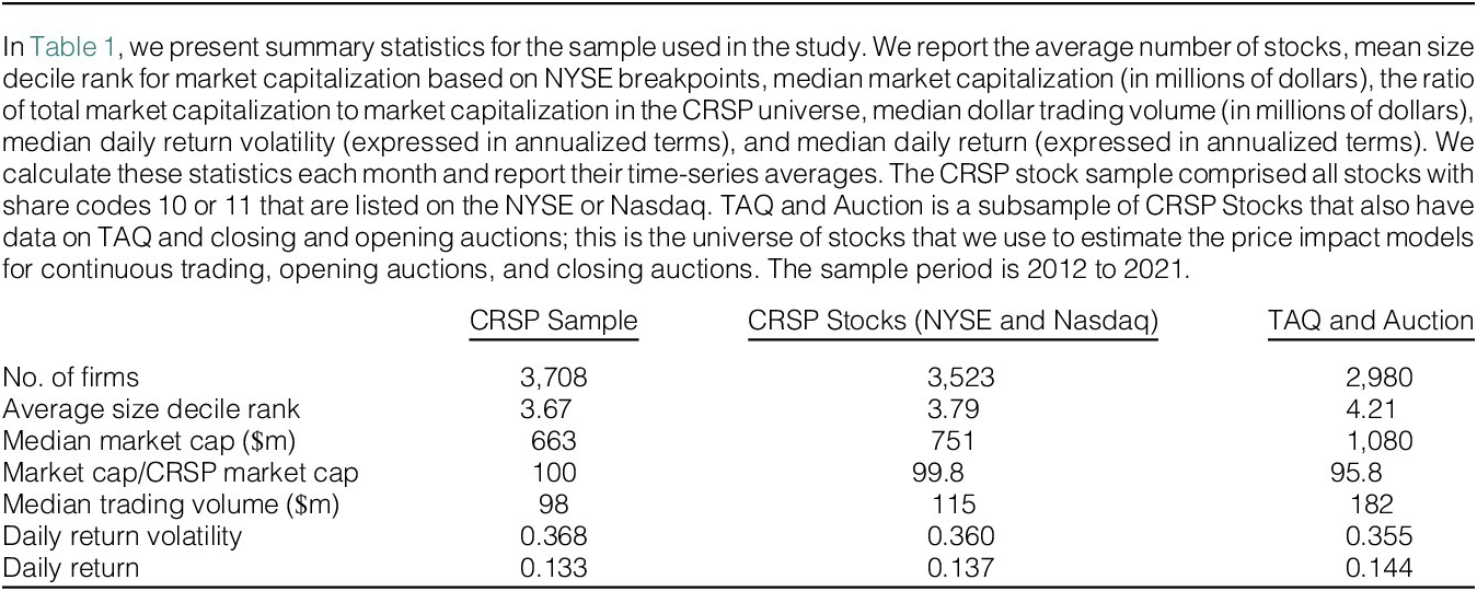
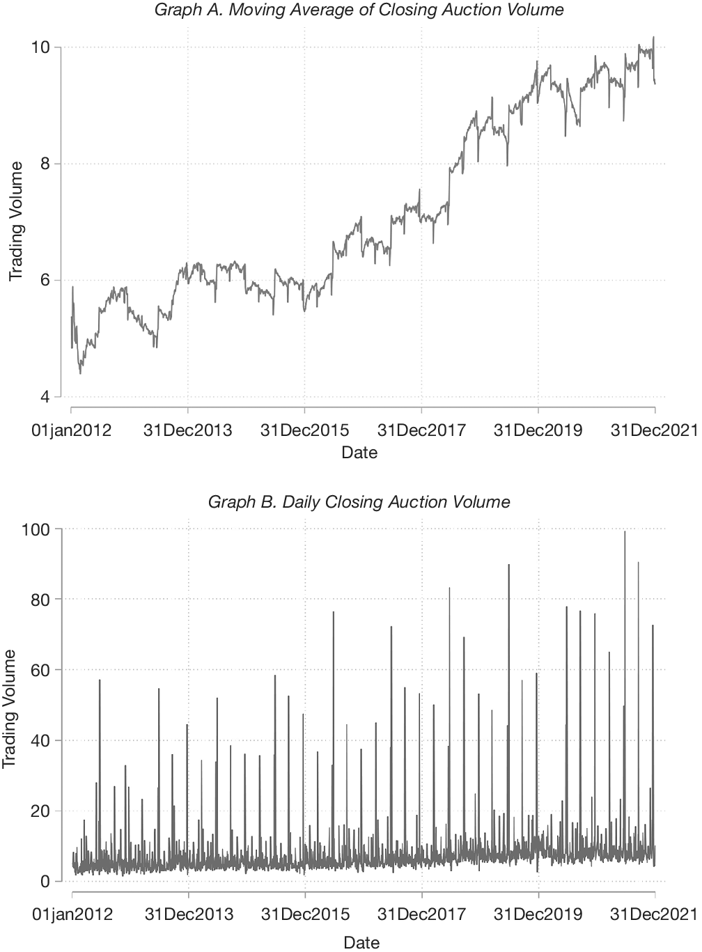
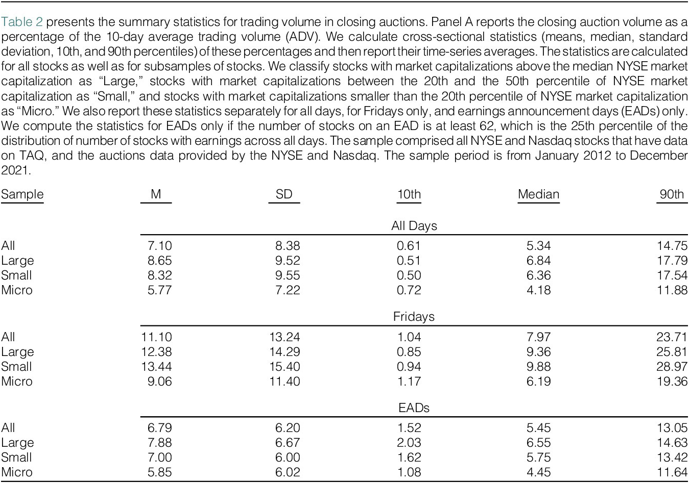


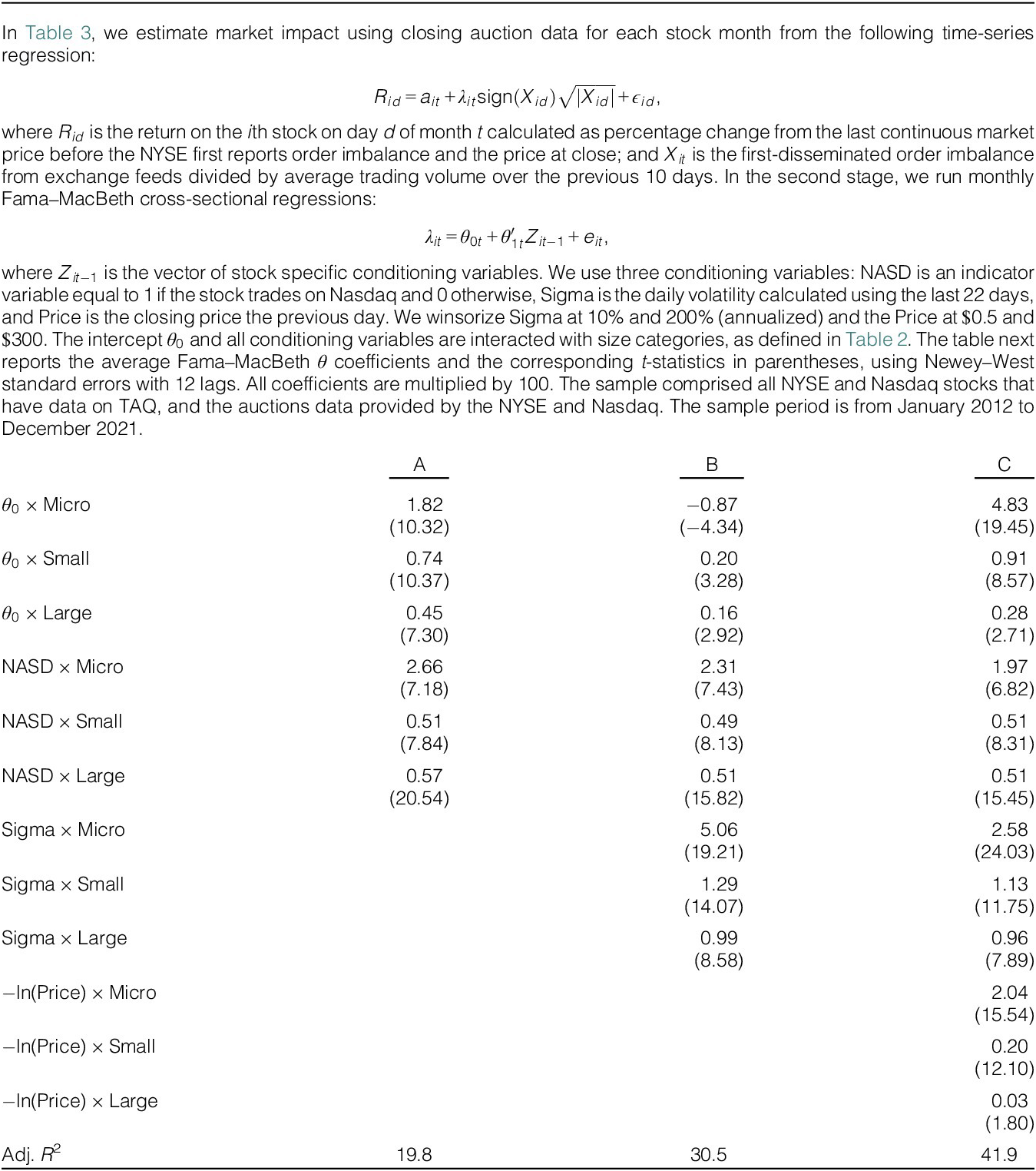

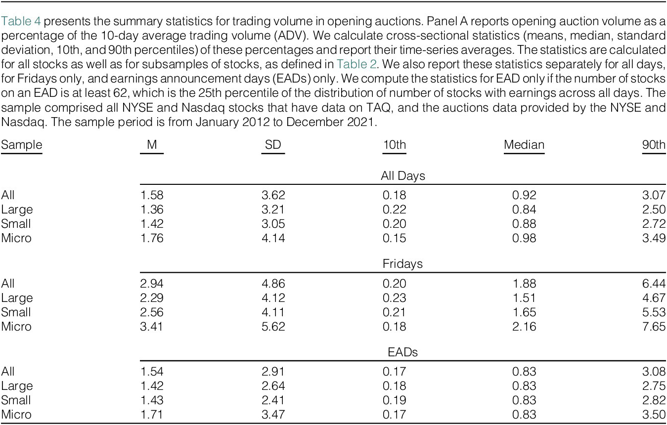
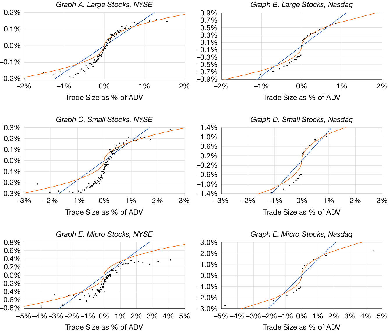
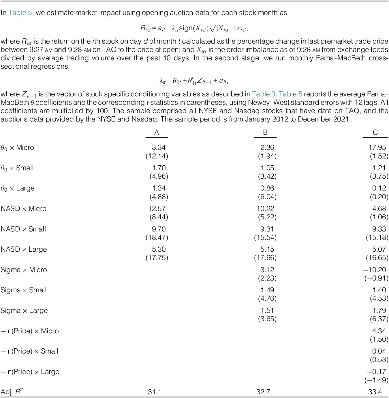
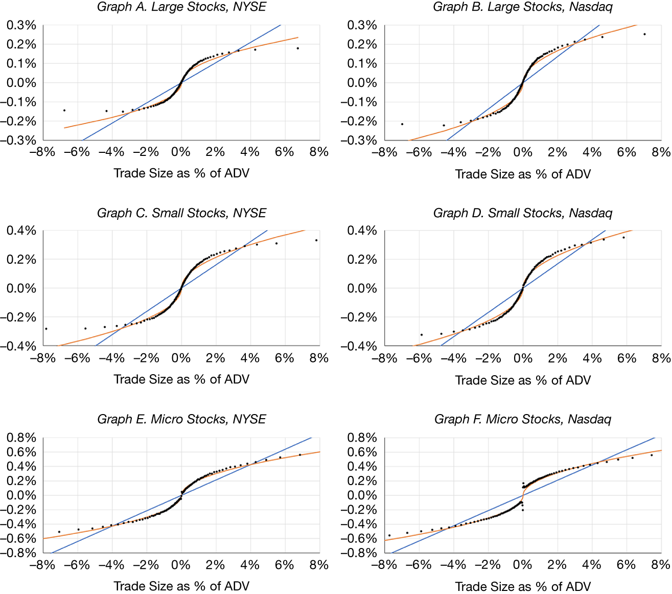

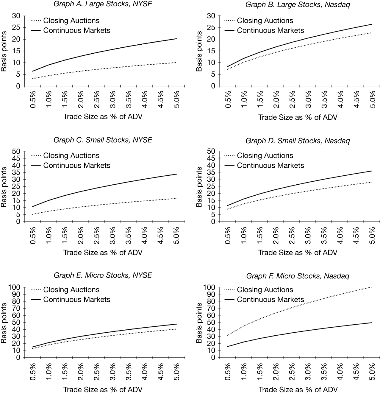
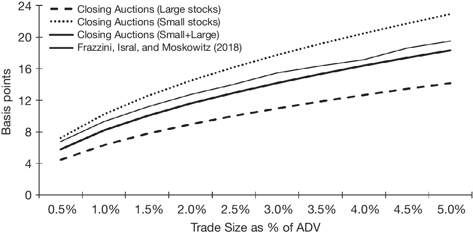
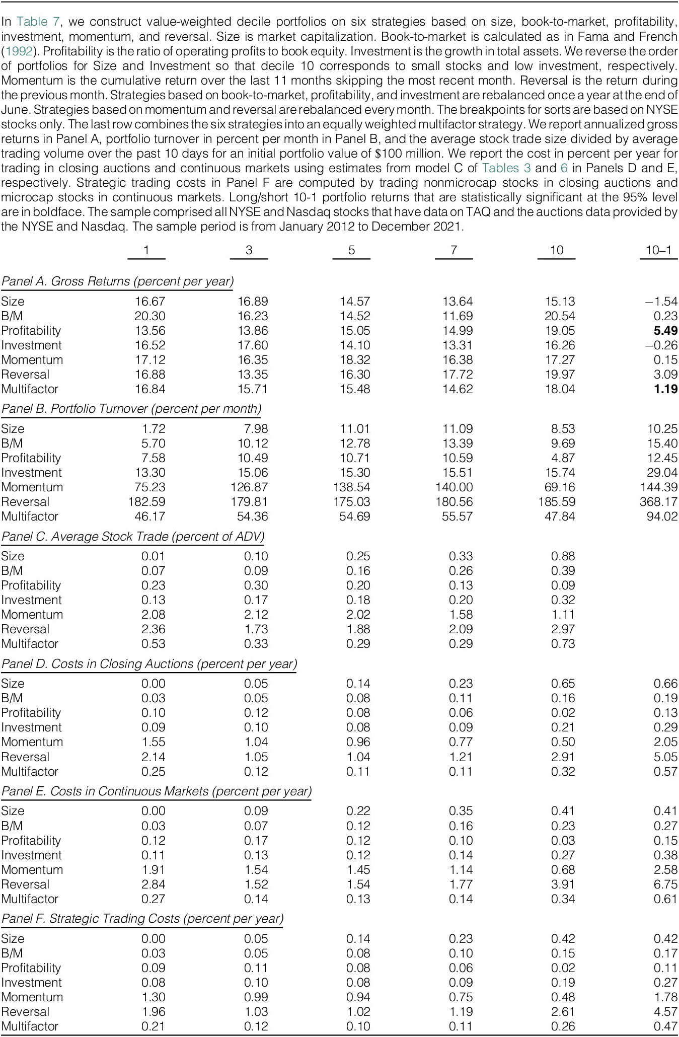

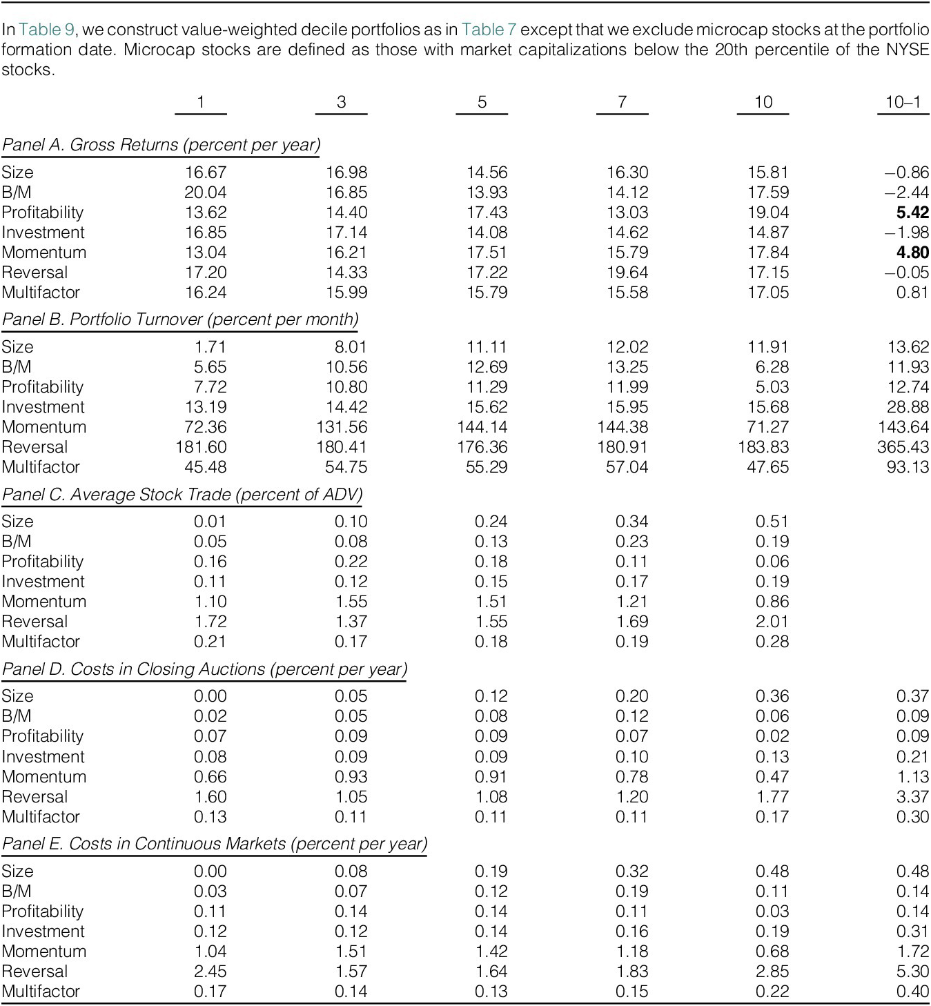
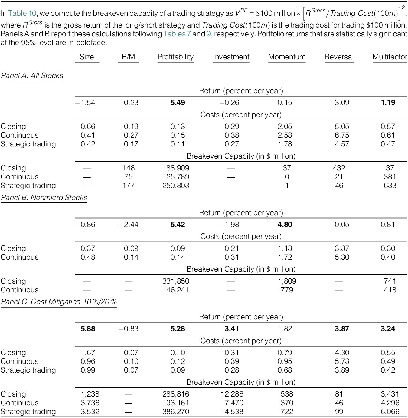


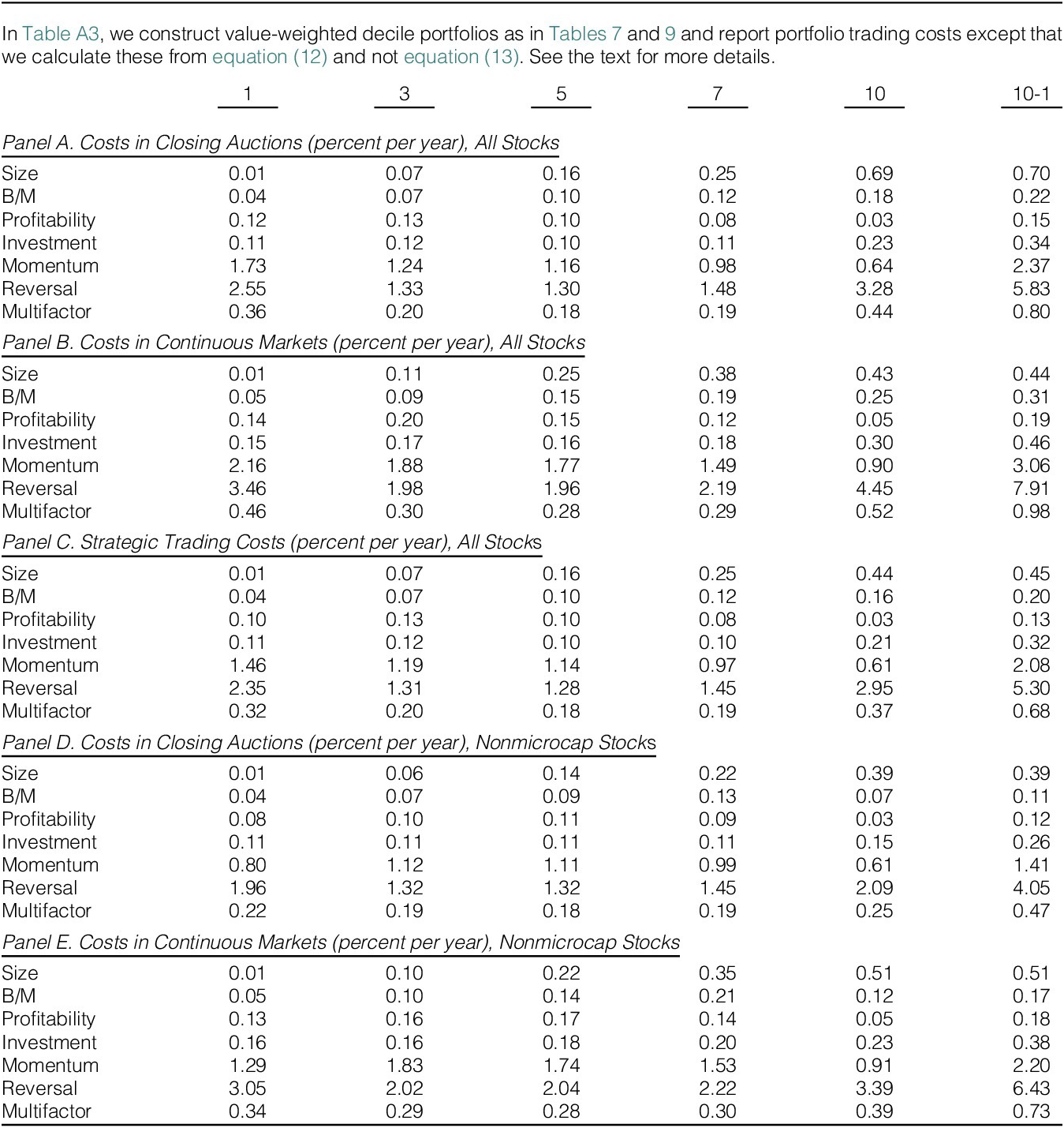

 Open access