
 −k
−k





1. Introduction
Symmetry, the invariance of a system under specific transformations, constitutes a cornerstone in facilitating understanding of the natural world (Gross Reference Gross1996). Conservation of various observable quantities (Noether Reference Noether1918), the fundamental forces of nature (Nambu & Jona-Lasinio Reference Nambu and Jona-Lasinio1961; Kobayashi & Maskawa Reference Kobayashi and Maskawa1973), constancy of the laws of physics from one inertial frame to another (Einstein Reference Einstein1905) and their indifference to choice of coordinate system (Einstein Reference Einstein1916), may all be ascribed to manifestations of different types of symmetry present in the universe. Additionally, the breaking of symmetry in a system is a well-known property of phase transitions (Landau Reference Landau1937; Onsager Reference Onsager1944; Bardeen et al. Reference Bardeen, Cooper and Schrieffer1957a , Reference Bardeen, Cooper and Schriefferb ), and also the very means by which particles are given mass (Higgs Reference Higgs1964). In fluid mechanics the Kolmogorov model of turbulence (Kolmogorov Reference Kolmogorov1941) describes an ideal and conservative cascade of energy through an inertial range of scales that arises due to inherent symmetry present in the advective fluid nonlinearity (Obukhov et al. Reference Obukhov1949) (in the absence of viscous dissipation) responsible for the otherwise complicated dynamics of these types of systems.
Nonlinear fluid advection and turbulence also arise in magnetic fusion devices, where the presence of strong gradients in quantities such as temperature and particle density instigate the bulk motions that carry thermal energy and matter out of the core of the reactor, resulting in significant loss of confinement. The associated problem of mitigating, minimising and controlling gradient-driven turbulent transport remains a palpable issue confronting the break-even capabilities of any such device (Garbet et al. Reference Garbet2004). One of the most significant occurrences of this type of phenomenon is associated with the ion temperature gradient (ITG) instability (Rudakov & Sagdeev Reference Rudakov and Sagdeev1961; Coppi, Rosenbluth & Sagdeev Reference Coppi, Rosenbluth and Sagdeev1967; Terry, Anderson & Horton Reference Terry, Anderson and Horton1982; Rosenbluth & Hinton Reference Rosenbluth and Hinton1998; Horton Reference Horton2017). In tokamaks, the ITG instability is one of the primary means by which drift waves (gyroradius-scale oscillations driven by density and temperature gradients; see, for instance, Horton Reference Horton1999) are driven to sufficiently large amplitudes that they enter a nonlinear regime, and a turbulent state arises (Horton et al. Reference Horton, Choi and Tang1981, Reference Horton, Hong and Tang1988; Horton Reference Horton2017).
A characteristic feature of ITG-driven turbulence is the generation of zonal flows (ZFs) (Rosenbluth & Hinton Reference Rosenbluth and Hinton1998; Rogers, Dorland & Kotschenreuther Reference Rogers, Dorland and Kotschenreuther2000), large-scale zero-frequency coherent structures with zero poloidal and toroidal mode numbers ( $m=n=0$
), which helically wind around the torus, tracking the flux surfaces to which they are localised. (For a more detailed review and explanation of ZFs, see Diamond et al. (Reference Diamond, Itoh, Itoh and Hahm2005), Itoh et al. (Reference Itoh, Itoh, Diamond, Hahm, Fujisawa, Tynan, Yagi and Nagashima2006), Galperin & Read (Reference Galperin and Read2019).) In general, ZFs do not experience growth due to linear instability, but rather are a byproduct of nonlinear interactions amongst drift waves. In particular, it has been demonstrated that they are the primary catalyst for interactions transferring energy from unstable to stable modes, the dominant mechanism for saturation of the toroidal ITG instability (Makwana et al. Reference Makwana, Terry and Kim2012, Reference Makwana, Terry, Pueschel and Hatch2014). Being that the formation and existence of ZFs in these types of systems are dependent upon reception of energy from other modes (as opposed to directly drawing free energy from the temperature gradient), the means by which their nonlinear growth saturates is an important and non-trivial question.
$m=n=0$
), which helically wind around the torus, tracking the flux surfaces to which they are localised. (For a more detailed review and explanation of ZFs, see Diamond et al. (Reference Diamond, Itoh, Itoh and Hahm2005), Itoh et al. (Reference Itoh, Itoh, Diamond, Hahm, Fujisawa, Tynan, Yagi and Nagashima2006), Galperin & Read (Reference Galperin and Read2019).) In general, ZFs do not experience growth due to linear instability, but rather are a byproduct of nonlinear interactions amongst drift waves. In particular, it has been demonstrated that they are the primary catalyst for interactions transferring energy from unstable to stable modes, the dominant mechanism for saturation of the toroidal ITG instability (Makwana et al. Reference Makwana, Terry and Kim2012, Reference Makwana, Terry, Pueschel and Hatch2014). Being that the formation and existence of ZFs in these types of systems are dependent upon reception of energy from other modes (as opposed to directly drawing free energy from the temperature gradient), the means by which their nonlinear growth saturates is an important and non-trivial question.
While lacking linear growth, it is commonplace in analytic and computational modelling to include linear dissipation of ZFs to assist in mediating saturation and numerical convergence. It has been observed in gyrokinetic simulations and analytic calculations that the total turbulent energy and transport are proportional to linear ZF damping (Lin et al. Reference Lin, Hahm, Lee, Tang and Diamond1999; Colyer et al. Reference Colyer, Schekochihin, Parra, Roach, Barnes, Ghim and Dorland2017; Terry et al. Reference Terry, Faber, Hegna, Mirnov, Pueschel and Whelan2018). However, we note that there exist cases for which the collisionless damping of zonal modes also appears to affect these quantities (Waltz & Holland Reference Waltz and Holland2008). In addition to potentially constraining turbulent energy levels, it has been observed for the model employed herein that collisional damping breaks dynamic and energetic symmetry between unstable and stable modes (Terry et al. Reference Terry, Faber, Hegna, Mirnov, Pueschel and Whelan2018). The exponential growth of unstable modes (due to linear instability) in a system is offset by exponential damping due to its nonlinearly excited stable modes and ZFs. The latter take a subdominant role in energetic dissipation, but play an important part in exploiting the symmetry between unstable/stable eigenmodes (Terry et al. Reference Terry, Faber, Hegna, Mirnov, Pueschel and Whelan2018). At a given wavevector $\boldsymbol{k}$
, a stable eigenmode will damp energy at a slightly faster rate than its nearly conjugate unstable counterpart, and saturation arises with unstable-mode energy at any given
$\boldsymbol{k}$
, a stable eigenmode will damp energy at a slightly faster rate than its nearly conjugate unstable counterpart, and saturation arises with unstable-mode energy at any given $\boldsymbol{k}$
slightly larger than stable-mode energy. This deviation from precise equality occurs in proportion to ZF collisionality.
$\boldsymbol{k}$
slightly larger than stable-mode energy. This deviation from precise equality occurs in proportion to ZF collisionality.
How ZFs saturate in the absence of collisionality remains an open question in drift-wave turbulence theory. This limit corresponds to the growth (which is always nonlinear) being arrested by purely nonlinear processes. While the mathematical model employed in this work, as well as more comprehensive approaches such as gyrokinetics, predict zero heat flux in the collisionless limit, simulations of these systems nonetheless exhibit finite fluxes. This raises the question of whether gyrokinetic simulations that incorporate the aforementioned sources of artificial dissipation can genuinely be considered collisionless. To the author’s knowledge, this has not yet been explored in the literature. In particular, we proceed by considering the problem from the perspective of partial differential equations (PDEs) and dynamical systems.
In the strictly collisionless limit, the gyrokinetic equations define a conservative, phase-space–volume–preserving system. At the PDE level, this corresponds to a fully hyperbolic dynamical system, in which no intrinsic mechanism exists to select asymptotic states. Such systems do not generically evolve toward attractors; instead, they retain memory of initial conditions and permit a persistent fine-scale structure. Crucially, this regime is not what is realised in essentially all practical gyrokinetic simulations. Even in nominally collisionless studies, hyperviscosity or related forms of artificial dissipation are invariably present. The introduction of these terms changes the equations from purely hyperbolic to mixed hyperbolic–parabolic. This is not a small perturbation: it qualitatively alters the solution space by introducing irreversible dynamics, suppressing fine-scale structure and selecting attractor-like behaviour. In doing so, it enforces saturation through dissipative pathways (e.g. cascade to high wavenumber), thereby precluding or obscuring saturation mechanisms that depend on exact conservation and symmetry.
In the analytic model used herein, the limit of zero ZF damping results in symmetrisation of the linear eigenvalues for the unstable/stable eigenmodes of the system (Terry et al. Reference Terry, Faber, Hegna, Mirnov, Pueschel and Whelan2018). This is associated with parity-time (PT) symmetry in the underlying ITG fluid model equations. Its presence raises the familiar question in physics of whether such a property can be exploited in various ways to infer relatively straightforward analytic solutions and phenomenology. This idea forms the backbone of the analysis presented herein. Recently, PT symmetry has been used to investigate similar systems in the context of non-Hermitian dynamics (Bentzien, Pinske & Maczewsky Reference Bentzien, Pinske and Maczewsky2025) as well as turbulent fluids (Fu & Qin Reference Fu and Qin2020; Qin et al. Reference Qin, Fu, Glasser and Yahalom2021; de Wit et al. Reference de Wit, Galtier, Fruchart, Toschi and Vitelli2025). In this work, it is shown that the aforementioned symmetry results in relatively simple characterisation of collisionless ZF saturation involving balanced contributions to the ZF from unstable and stable modes.
In this work, an instability-driven weak-turbulence closure technique (Malfliet Reference Malfliet1972) is applied to a reduced two-field model for ITG-driven turbulence (Horton et al. Reference Horton, Choi and Tang1981, Reference Horton, Hong and Tang1988; Holland et al. Reference Holland, Diamond, Champeaux, Kim, Gurcan, Rosenbluth, Tynan, Crocker, Nevins and Candy2003; Terry et al. Reference Terry, Faber, Hegna, Mirnov, Pueschel and Whelan2018) that has been truncated to three wavevectors and five modes (Li & Terry Reference Li and Terry2022, Reference Li and Terry2024). The closure calculation produces a ZF wave kinetic equation (WKE), which yields a time-evolution operator that characterises the manner in which the energy in these types of modes will vary due to both linear and nonlinear processes. The latter group corresponds to turbulence in the form of resonant interactions among triads of fluctuations; in essence, these terms represent the non-trivial component of the ZF Hamiltonian. In an effort to elucidate the nature of the nonlinearity, these portions of the time-evolution operator are expressed as tensors made of simple arithmetic combinations of the far more familiar individual linear eigenvalues of the interacting modes. When viewed in this light, the collective nonlinear behaviour of this system of interacting modes (referred to as turbulence), appears merely to be the result of amalgamating their innate tendencies (linear wave oscillation and growth/decay) when observed in isolation from one another. The limit of zero ZF collisionality is then applied to the WKE and associated time-evolution tensors. In this limit, the linear eigenvalues of stable and unstable modes become complex-conjugate pairs, a property that propagates through the aforementioned weak-turbulence closure calculation, manifesting as centrosymmetry in the time-evolution tensors describing the nonlinear behaviour of the modes. Stationary solutions to the WKE in the collisionless limit are then found, which describe ZFs that saturate when energy is equally partitioned between the unstable and conjugate stable mode at each $\boldsymbol{k}$
. Phenomenologically, this condition is shown to coincide with transport for which the amount of thermal energy being moved down gradient over each characteristic length scale (
$\boldsymbol{k}$
. Phenomenologically, this condition is shown to coincide with transport for which the amount of thermal energy being moved down gradient over each characteristic length scale ( $k^{-1}$
) is on average perfectly balanced by energy moving in the opposite direction; the collisionless ZF saturation mechanism corresponds to an equilibrium state describing an ‘idealised’ confinement of heat. This outcome is thermodynamically allowed because with zero collisionality the entropy is constant (Sugama & Horton Reference Sugama and Horton1997; Abel et al. Reference Abel, Plunk, Wang, Barnes, Cowley, Dorland and Schekochihin2013). It is important to stress that this result is shown to hold in a statistical sense. The heat flux averages to zero over sufficiently many nonlinear time scales over which there are alternating periods of up- and down-gradient transport. For more realistic systems with small but finite collisionality, these results suggest that ITG-driven turbulence tends toward a state in which energy is increasingly equally partitioned between counter-transporting fluctuations at each characteristic length scale as collisionality decreases. In the limit of vanishing collisionality, this behaviour approaches the exact equipartition predicted by the idealised collisionless theory. Lastly, the ZF WKE for the untruncated system is briefly mentioned and contrasted with the analysis for the truncated system.
$k^{-1}$
) is on average perfectly balanced by energy moving in the opposite direction; the collisionless ZF saturation mechanism corresponds to an equilibrium state describing an ‘idealised’ confinement of heat. This outcome is thermodynamically allowed because with zero collisionality the entropy is constant (Sugama & Horton Reference Sugama and Horton1997; Abel et al. Reference Abel, Plunk, Wang, Barnes, Cowley, Dorland and Schekochihin2013). It is important to stress that this result is shown to hold in a statistical sense. The heat flux averages to zero over sufficiently many nonlinear time scales over which there are alternating periods of up- and down-gradient transport. For more realistic systems with small but finite collisionality, these results suggest that ITG-driven turbulence tends toward a state in which energy is increasingly equally partitioned between counter-transporting fluctuations at each characteristic length scale as collisionality decreases. In the limit of vanishing collisionality, this behaviour approaches the exact equipartition predicted by the idealised collisionless theory. Lastly, the ZF WKE for the untruncated system is briefly mentioned and contrasted with the analysis for the truncated system.
Models such as the Hasegawa–Mima equation and other reduced fluid systems (Charney Reference Charney1948; Hasegawa & Mima Reference Hasegawa and Mima1978; Hasegawa & Wakatani Reference Hasegawa and Wakatani1987) have been used to analytically and numerically investigate drift-wave turbulence in considerable detail (Champeaux & Diamond Reference Champeaux and Diamond2001; Lashmore-Davies et al. Reference Lashmore-Davies, McCarthy and Thyagaraja2001; Manfredi et al. Reference Manfredi, Roach and Dendy2001; Jenko Reference Jenko2006; Lashkin Reference Lashkin2008; Connaughton et al. Reference Connaughton, Nadiga, Nazarenko and Quinn2010; Gallagher et al. Reference Gallagher, Hnat, Connaughton, Nazarenko and Rowlands2012; Connaughton et al. Reference Connaughton, Nazarenko and Quinn2015; Zhu et al. Reference Zhu, Zhou and Dodin2019), with a variety of techniques being employed, including the methods of modulational instability (Piliptetskii & Rustamov Reference Piliptetskii and Rustamov1965; Bespalov & Talanov Reference Bespalov and Talanov1966; Yuen & Lake Reference Yuen and Lake1980) and weak turbulence (Malfliet Reference Malfliet1972; Zakharov et al. Reference Zakharov, L’Vov and Falkovich1992; Nazarenko Reference Nazarenko2011; Galtier Reference Galtier2023b ). The work presented herein differs from prior analytic studies of collisionless ZFs due to the particular choices of the weak-turbulence closure method (Malfliet Reference Malfliet1972), the use of the reduced two-field fluid model for toroidal ITG turbulence (Horton et al. Reference Horton, Choi and Tang1981, Reference Horton, Hong and Tang1988; Holland et al. Reference Holland, Diamond, Champeaux, Kim, Gurcan, Rosenbluth, Tynan, Crocker, Nevins and Candy2003) and the decomposition of the fluctuation fields into stable and unstable eigenmodes (Makwana et al. Reference Makwana, Terry and Kim2012, Reference Makwana, Terry, Pueschel and Hatch2014; Terry et al. Reference Terry, Faber, Hegna, Mirnov, Pueschel and Whelan2018). In addition, an intuitive collisionless saturation mechanism, with corresponding phenomenology expressed in terms of the turbulent transport is suggested. In this mechanism the energy extracted from the instability-driving gradient by unstable modes is returned to the gradient at an equal rate by nonlinearly excited conjugate stable modes.
This is the first of two papers in a series on a saturation theory for collisionless ITG-driven turbulence. This paper is primarily an exercise in analytic theory, deriving a ZF WKE and predicting the conditions under which this mode saturates in terms of the system’s modal energy spectra. In Part II we will present analogous calculations for the eigenmode energies and the conditions under which these modes saturate. In addition, numerical simulations of both the $3-\boldsymbol{k}$
and many
$3-\boldsymbol{k}$
and many $-\boldsymbol{k}$
systems will be used to confirm the predictions of the theory.
$-\boldsymbol{k}$
systems will be used to confirm the predictions of the theory.
The rest of the paper is structured as follows. Section 2 introduces a reduced two-field fluid model for toroidal ITG turbulence. The model is transformed to a representation in terms of its stable/unstable eigenmodes and subjected to a three-wavevector truncation. Section 3 presents the result of application of a weak-turbulence closure to the reduced two-field fluid model to obtain a WKE for ZF spectral time evolution. Section 4 analyses the structure of the tensors constituting nonlinear time evolution found in the ZF WKE. Section 5 calculates some sets of states for which the ZF WKE exhibits stationarity and relates them to the turbulent transport. Lastly, § 6 comments briefly on generalisation of the results to systems with many $\boldsymbol{k}$
s (
$\boldsymbol{k}$
s ( ${\gt} 3$
).
${\gt} 3$
).
2. Fluid models
A two-field fluid model for toroidal ITG turbulence describing the nonlinear temporal evolution of electrostatic potential $\phi _k=\phi (k_x,k_y)$
and pressure
$\phi _k=\phi (k_x,k_y)$
and pressure $p_k=p(k_x,k_y)$
is used to analytically investigate ZF saturation mechanisms. The model may be expressed as a spatially Fourier transformed pair of coupled nonlinear PDEs of the form
$p_k=p(k_x,k_y)$
is used to analytically investigate ZF saturation mechanisms. The model may be expressed as a spatially Fourier transformed pair of coupled nonlinear PDEs of the form
 \begin{align} \frac {\partial p_k}{\partial t} + ik_y(1+\eta )\phi _k + \chi k_\perp ^4 p_k = - \sum _{\boldsymbol{k}^{\prime }} (\boldsymbol{k}^{\prime } \times \hat {z} \boldsymbol{\cdot }\boldsymbol{k})\phi _{\boldsymbol{k}^{\prime }}p_{\boldsymbol{k}^{\prime \prime }}, \end{align}
 \begin{align} \big[\delta (k_y)+k_\perp ^2\big]\frac {\partial \phi _k}{\partial t} & + ik_y \phi _k - i k_y \epsilon _n p_k + \nu k_\perp ^2 \phi _k = -\frac {1}{2} \sum _{k^{\prime }} (\boldsymbol{k}^{\prime } \times \hat {z} \boldsymbol{\cdot }\boldsymbol{k}) \big(\boldsymbol{k}_\perp ^{\prime \prime 2} - \boldsymbol{k}_\perp ^{{\prime } 2}\big)\phi _{k^{\prime }}\phi _{k^{\prime \prime }}\nonumber\\[4pt]& +\frac {1}{2} \sum _{k_x^{\prime }}k_y\big[k_x'\phi _{k^{\prime }}\phi _{k^{\prime \prime }}|_{k_y'=0}+(k_x-k_x')\phi _{k^{\prime }}\phi _{k^{\prime \prime }} |_{k_y'=k_y}\big] . \end{align}
Equations (2.1) and (2.2) describe two-dimensional turbulence that is strongly localised along a magnetic field line at the outboard midplane of a tokamak. The $x$
coordinate corresponds to the radial direction while
$x$
coordinate corresponds to the radial direction while $y$
is binormal. The model is spatially homogeneous because the density gradient is treated as constant and strong ballooning implies a localised mode structure to the outboard midplane (Horton, Choi & Tang Reference Horton, Choi and Tang1981). The parameter
$y$
is binormal. The model is spatially homogeneous because the density gradient is treated as constant and strong ballooning implies a localised mode structure to the outboard midplane (Horton, Choi & Tang Reference Horton, Choi and Tang1981). The parameter $\eta$
is the ratio of density to temperature gradient scale lengths,
$\eta$
is the ratio of density to temperature gradient scale lengths, $\epsilon _n$
is the inverse scale length of magnetic field curvature normalised to the density-gradient scale length,
$\epsilon _n$
is the inverse scale length of magnetic field curvature normalised to the density-gradient scale length, $\delta (k_y)$
is the adiabatic electron response, and
$\delta (k_y)$
is the adiabatic electron response, and $\nu$
and
$\nu$
and $\chi$
are coefficients of collisional dissipation. Length scales are normalised to the ratio of sound speed
$\chi$
are coefficients of collisional dissipation. Length scales are normalised to the ratio of sound speed $c_s = (T_e/m_i)^{1/2}$
to ion cyclotron frequency
$c_s = (T_e/m_i)^{1/2}$
to ion cyclotron frequency $\varOmega _{ci} = qB/m_i$
in the form
$\varOmega _{ci} = qB/m_i$
in the form $\rho _s=c_s/\varOmega _{ci}$
, such that
$\rho _s=c_s/\varOmega _{ci}$
, such that $k_\perp \rho _s \rightarrow k_\perp$
.
$k_\perp \rho _s \rightarrow k_\perp$
. $T_e$
is the electron temperature,
$T_e$
is the electron temperature, $m_i$
is the ion mass,
$m_i$
is the ion mass, $q$
is the charge of the ion and
$q$
is the charge of the ion and $B$
is the on-axis magnetic field strength. For modes with
$B$
is the on-axis magnetic field strength. For modes with $k_y=0$
, there is no adiabatic electron response, hence,
$k_y=0$
, there is no adiabatic electron response, hence,
 \begin{align} \delta (k_y)= \begin{cases} 0 & k_y =0 \\ 1 & k_y\neq 0 \end{cases}. \end{align}
This system is valid in the limit of low frequency relative to the ion cyclotron frequency, and strong ballooning of the fluctuation eigenfunction about the outboard midplane in a toroidal coordinate system transformed via the ballooning representation is assumed. For the electron dynamics, the system assumes adiabatic electrons. This model has been derived and refined in Horton et al. (Reference Horton, Choi and Tang1981), Horton, Hong & Tang (Reference Horton, Hong and Tang1988) and Holland et al. (Reference Holland, Diamond, Champeaux, Kim, Gurcan, Rosenbluth, Tynan, Crocker, Nevins and Candy2003), investigated mathematically and computationally in considerable depth and shown to make good agreement with features of gyrokinetic simulations (Holland et al. Reference Holland, Diamond, Champeaux, Kim, Gurcan, Rosenbluth, Tynan, Crocker, Nevins and Candy2003; Makwana et al. Reference Makwana, Terry and Kim2012, Reference Makwana, Terry, Pueschel and Hatch2014; Terry et al. Reference Terry, Faber, Hegna, Mirnov, Pueschel and Whelan2018, Reference Terry, Li, Pueschel and Whelan2021). (For more detailed discussions of this system, see Horton et al. (Reference Horton, Choi and Tang1981, Reference Horton, Hong and Tang1988), Holland et al. (Reference Holland, Diamond, Champeaux, Kim, Gurcan, Rosenbluth, Tynan, Crocker, Nevins and Candy2003) and Terry et al. (Reference Terry, Faber, Hegna, Mirnov, Pueschel and Whelan2018).) The second nonlinearity of (2.2) arises from the advection of the adiabatic electron response by the ZF. This nonlinearity was neglected in the aforementioned works; in an eigenmode decomposition its contribution to the nonlinearity is seen to be small for peaked density – of order $\epsilon _n$
relative to the dominant advection-of-ion-pressure nonlinearity. This nonlinearity is retained here for the sake of generality.
$\epsilon _n$
relative to the dominant advection-of-ion-pressure nonlinearity. This nonlinearity is retained here for the sake of generality.
It can be shown that the linear eigenmodes of this system at $k_y\neq 0$
are stable and unstable modes with eigenfrequencies
$k_y\neq 0$
are stable and unstable modes with eigenfrequencies $\omega _j$
, whose amplitudes are
$\omega _j$
, whose amplitudes are $\beta _2=\beta _2(\boldsymbol{k})$
and
$\beta _2=\beta _2(\boldsymbol{k})$
and $\beta _1=\beta _1(\boldsymbol{k})$
and whose eigenvector coefficients are
$\beta _1=\beta _1(\boldsymbol{k})$
and whose eigenvector coefficients are $R_2$
and
$R_2$
and $R_1$
. The amplitudes
$R_1$
. The amplitudes $\beta _1$
and
$\beta _1$
and $\beta _2$
are related to
$\beta _2$
are related to $\phi _k$
and
$\phi _k$
and $p_k$
via the transformation
$p_k$
via the transformation
 \begin{align} \begin{pmatrix} p_k \\[2pt] \phi _k \end{pmatrix} = \begin{pmatrix} R_1(\boldsymbol{k}) & \quad R_2(\boldsymbol{k}) \\[2pt] 1 & \quad 1 \end{pmatrix} \begin{pmatrix} \beta _1(\boldsymbol{k}) \\[2pt] \beta _2(\boldsymbol{k}) \end{pmatrix}\!, \end{align}
in terms of eigenvector coefficients
 \begin{align} R_j = \frac {-\omega _j\big(1+k_\perp ^2\big)+k_y[1+\epsilon _n(1-\sqrt {8})]-\mathrm{i}\nu k_\perp ^2}{ 2k_y \epsilon _n}. \end{align}
It is fairly commonplace in studies of fluid mechanical systems to decompose governing equations into their respective eigenmode representations (Lamb Reference Lamb1911; Cowling Reference Cowling1941; Elsasser Reference Elsasser1950; Tassoul Reference Tassoul1980; Lien & Müller Reference Lien and Müller1992; Terry et al. Reference Terry, Baver and Gupta2006, Reference Terry, Faber, Hegna, Mirnov, Pueschel and Whelan2018) and interpret the nonlinearity as interactions among the constituent linear eigenmodes (Kumar & Goldreich Reference Kumar and Goldreich1989; Galtier et al. Reference Galtier, Nazarenko, Newell and Pouquet2001; Terry et al. Reference Terry, Baver and Gupta2006, Reference Terry, Faber, Hegna, Mirnov, Pueschel and Whelan2018; Azelis et al. Reference Azelis, Perez and Bourouaine2024; Remond-Tiedrez et al. Reference Remond-Tiedrez, Smith and Stechmann2024; Van Beeck et al. Reference Van Beeck, Van Hoolst, Aerts and Fuller2024).
Transforming a system to be expressed in terms of its linear eigenfunctions and eigenvalues often simplifies the mathematical structure of the governing equations. It is a standard technique (introduced in undergraduate physics texts) that is broad in applicability and can readily be applied to many different systems. Its mathematical implementation is not overly preoccupied with what particular physical processes are occurring. Despite this, it allocates considerable physical intuition with which to characterise nonlinear dynamics using the language of the more familiar and easily comprehensible linear physics of the system. For instance, the eigenmode decomposition proposed by Elsasser (Reference Elsasser1950) readily allows for the nonlinearity of the incompressible magnetohydrodynamic system to be understood as interactions between counter-propagating Alfvénic fluctuations (Galtier et al. Reference Galtier, Nazarenko, Newell and Pouquet2001). This is in contrast with potentially esoteric notions of considering all the ways in which velocity and magnetic fields may interact with themselves and each other.
The eigenmode decomposition used in this work casts the dynamics in terms of fluctuations that transport energy up and down the temperature gradient in the form of stable and unstable modes, respectively. In addition, casting the fluid model in terms of these modes allows for immediate inference and quantification of the rates at which energy is being added to and removed from the system of modes due to its interactions with a mean temperature gradient. In the context of fusion-relevant turbulence, where the central issues are stability and confinement degradation, this decomposition offers a particularly natural and physically transparent framework. Its utility has been tested in comparisons with the singular value decomposition, bases with and without dissipation, bases that evolve with relaxing profiles in decaying turbulence and bases that are intrinsically nonlinear. Its utility and transparency is evident in many situations.
It has been previously shown that the toroidal branch of the ITG instability saturates via ZF-catalysed energy transfer from the unstable mode to the stable mode (Hatch et al. Reference Hatch, Terry, Jenko, Merz and Nevins2011; Makwana et al. Reference Makwana, Terry and Kim2012, Reference Makwana, Terry, Pueschel and Hatch2014; Terry et al. Reference Terry, Faber, Hegna, Mirnov, Pueschel and Whelan2018; Li & Terry Reference Li and Terry2022). This particular mechanism also plays a prominent role in dictating other nonlinear dynamical aspects of these types of systems (Whelan et al. Reference Whelan, Pueschel and Terry2018, Reference Whelan, Pueschel, Terry, Citrin, McKinney, Guttenfelder and Doerk2019; Terry et al. Reference Terry, Li, Pueschel and Whelan2021; Li & Terry Reference Li and Terry2022). Saturation by ZF-catalysed nonlinear energy transfer to stable modes is also observed in turbulence driven by the Kelvin–Helmholtz (Fraser et al. Reference Fraser, Terry, Zweibel, Pueschel and Schroeder2021; Tripathi et al. Reference Tripathi, Fraser, Terry, Zweibel and Pueschel2022a , Reference Tripathi, Fraser, Terry, Zweibel and Pueschelb , Reference Tripathi, Fraser, Terry, Zweibel, Pueschel and Anders2023a , Reference Tripathi, Terry, Fraser, Zweibel and Pueschelb ), Goldreich–Schubert–Fricke (Tripathi et al. Reference Tripathi, Barker, Fraser, Terry and Zweibel2024) and semi-collisional trapped electron mode instabilities (Terry et al. Reference Terry, Gatto and Baver2002). More generally, in the absence of ZFs, saturation by nonlinear energy transfer to stable modes is a common feature of fluid models for instability-driven turbulence (Makwana et al. Reference Makwana, Terry, Kim and Hatch2011). This paradigm also arises in both trapped electron mode turbulence (Baver et al. Reference Baver, Terry, Gatto and Fernandez2002; Terry et al. Reference Terry, Baver and Gupta2006) and electron temperature gradient-driven turbulence (Kim & Terry Reference Kim and Terry2010).
In the present analysis, we are interested in the wavenumber range where $k_\perp ^2 \ll 1$
, and use this to further assume that
$k_\perp ^2 \ll 1$
, and use this to further assume that $\chi k_\perp ^2 \ll \nu$
(Terry et al. Reference Terry, Li, Pueschel and Whelan2021). The limit of small
$\chi k_\perp ^2 \ll \nu$
(Terry et al. Reference Terry, Li, Pueschel and Whelan2021). The limit of small $k_\perp$
is taken as a simplifying approximation that is valid because the instability is driven and saturated by stable modes in the regime
$k_\perp$
is taken as a simplifying approximation that is valid because the instability is driven and saturated by stable modes in the regime $k_\perp ^2 \ll 1$
. However, mode dispersion, which enters from the ion polarisation drift, is necessary because otherwise the nonlinear triplet interaction time becomes infinite under the resonant vanishing of the frequency mismatch for non-dispersive waves. This means that the lowest-order contribution to the frequency mismatch for zero collisionality is order
$k_\perp ^2 \ll 1$
. However, mode dispersion, which enters from the ion polarisation drift, is necessary because otherwise the nonlinear triplet interaction time becomes infinite under the resonant vanishing of the frequency mismatch for non-dispersive waves. This means that the lowest-order contribution to the frequency mismatch for zero collisionality is order $k_\perp ^2$
. This limit is taken consistently, as shown by the ordering scheme given in Terry et al. (Reference Terry, Faber, Hegna, Mirnov, Pueschel and Whelan2018). This scheme yields both an internally consistent expansion, and is consistent with general numerical solutions of the many-wavenumber two-field fluid system as described by Makwana, Terry & Kim (Reference Makwana, Terry and Kim2012). Given the above, the eigenvalues
$k_\perp ^2$
. This limit is taken consistently, as shown by the ordering scheme given in Terry et al. (Reference Terry, Faber, Hegna, Mirnov, Pueschel and Whelan2018). This scheme yields both an internally consistent expansion, and is consistent with general numerical solutions of the many-wavenumber two-field fluid system as described by Makwana, Terry & Kim (Reference Makwana, Terry and Kim2012). Given the above, the eigenvalues $\omega _j$
can be written as
$\omega _j$
can be written as
 \begin{align} \omega _{1,2} &= \frac {\epsilon _n k_y\big[2+(1+\sqrt {8})k_\perp ^2\big]+k_y - \mathrm{i}\nu k_\perp ^2}{2\big(1+k_\perp ^2\big)} \nonumber \\[4pt] &\pm \frac {\sqrt {-8 \epsilon _n k_y^2(1+\eta )\big(1+k_\perp ^2\big)+\big\{\epsilon _n k_y\big[2\sqrt {8}+(1+\sqrt {8})k_\perp ^2\big]-k_y+\mathrm{i}\nu k_\perp ^2\big\}^2}}{2\big(1+k_\perp ^2\big)}. \end{align}
Note that subscripts $1$
and
$1$
and $2$
refer to unstable/stable eigenmode labels throughout this work. The eigenvalues given by (2.6) follow from the linear dispersion relation (DR) for stable and unstable modes of this system. These modes have drift-wave oscillation, instability growth due to the temperature gradient
$2$
refer to unstable/stable eigenmode labels throughout this work. The eigenvalues given by (2.6) follow from the linear dispersion relation (DR) for stable and unstable modes of this system. These modes have drift-wave oscillation, instability growth due to the temperature gradient $\eta$
and magnetic curvature
$\eta$
and magnetic curvature $\epsilon _n$
, an ITG-stabilising effect induced by the density gradient
$\epsilon _n$
, an ITG-stabilising effect induced by the density gradient $L_n^{-1}$
and collisional damping due to
$L_n^{-1}$
and collisional damping due to $\nu$
. It should be noted that
$\nu$
. It should be noted that $\nu$
acts on both the turbulence and ZFs. Furthermore,
$\nu$
acts on both the turbulence and ZFs. Furthermore, $\omega _j$
is often algebraically manipulated throughout this work using the generic complex-number form
$\omega _j$
is often algebraically manipulated throughout this work using the generic complex-number form
 \begin{align} \omega _j = \varpi _j \pm \mathrm{i} \gamma _j \end{align}
for wave frequency $\varpi _j = \mathrm{Re}(\omega _j)$
and unstable/stable growth/damping rate
$\varpi _j = \mathrm{Re}(\omega _j)$
and unstable/stable growth/damping rate $\gamma _j=\mathrm{Im}(\omega _j)$
.
$\gamma _j=\mathrm{Im}(\omega _j)$
.
The dominant mechanism for saturation of the ITG instability in the models presented herein (Horton et al. Reference Horton, Choi and Tang1981, Reference Horton, Hong and Tang1988; Holland et al. Reference Holland, Diamond, Champeaux, Kim, Gurcan, Rosenbluth, Tynan, Crocker, Nevins and Candy2003; Li & Terry Reference Li and Terry2022) is ZF-catalysed energy transfer from the unstable to stable mode, for which $\gamma _j\neq 0$
(Terry et al. Reference Terry, Faber, Hegna, Mirnov, Pueschel and Whelan2018; Li & Terry Reference Li and Terry2022). In the interest of preserving the key turbulent saturation physics while using the wavenumber-truncated model, we restrict our analysis to choices of eigenmode wavevectors
$\gamma _j\neq 0$
(Terry et al. Reference Terry, Faber, Hegna, Mirnov, Pueschel and Whelan2018; Li & Terry Reference Li and Terry2022). In the interest of preserving the key turbulent saturation physics while using the wavenumber-truncated model, we restrict our analysis to choices of eigenmode wavevectors $\boldsymbol{k}$
and
$\boldsymbol{k}$
and $\boldsymbol{k}^{\prime \prime }$
for which
$\boldsymbol{k}^{\prime \prime }$
for which $\gamma _j = \mathrm{Im}(\omega _j) \neq 0$
. For suitable choices of
$\gamma _j = \mathrm{Im}(\omega _j) \neq 0$
. For suitable choices of $\epsilon _n$
(approximately
$\epsilon _n$
(approximately $.6 \lt \epsilon _n \lt 1.25$
) and
$.6 \lt \epsilon _n \lt 1.25$
) and $\eta$
above the threshold of linear instability, these appropriate
$\eta$
above the threshold of linear instability, these appropriate $\boldsymbol{k}$
s correspond to the radicand of (2.6) being negative. When
$\boldsymbol{k}$
s correspond to the radicand of (2.6) being negative. When $\nu =0$
, these are points in the
$\nu =0$
, these are points in the $k_xk_y$
plane satisfying
$k_xk_y$
plane satisfying
 \begin{align} -8 \epsilon _n k_y^2(1+\eta )\big(1+k_\perp ^2\big)+\big\{\epsilon _n k_y\big[2\sqrt {8}+(1+\sqrt {8})k_\perp ^2\big]-k_y\big\}^2 \lt 0. \end{align}
It can be shown that this is the interior of a curve that is quartic in $\boldsymbol{k}_\perp$
. For
$\boldsymbol{k}_\perp$
. For $\boldsymbol{k}$
outside of this curve, the eigenmodes are at most (for
$\boldsymbol{k}$
outside of this curve, the eigenmodes are at most (for $k_y \neq 0$
) purely oscillatory dispersive waves and possess no linear behaviour otherwise (
$k_y \neq 0$
) purely oscillatory dispersive waves and possess no linear behaviour otherwise ( $k_y=0$
).
$k_y=0$
).
One particularly important feature of the DR is that $\omega _1$
and
$\omega _1$
and $\omega _2$
constitute a complex-conjugate pair when
$\omega _2$
constitute a complex-conjugate pair when $\nu =0$
. Both the wave frequencies
$\nu =0$
. Both the wave frequencies
 \begin{align} \varpi _{1,\nu =0} = \varpi _{2,\nu =0} = \varpi \end{align}
and growth/damping rates
 \begin{align} \gamma _{1,\nu =0} = \gamma _{2,\nu =0} = \gamma \end{align}
for pairs of eigenmodes become equal; their values become eigenmode label independent. For $\nu =0$
, the complex mode frequency can be expressed as
$\nu =0$
, the complex mode frequency can be expressed as
 \begin{align} \omega _{j,\nu =0} = \varpi \pm \mathrm{i} \gamma . \end{align}
It will prove useful to introduce the exchange matrix
 \begin{align} J_2 = \begin{bmatrix} 0 & \quad 1 \\[2pt] 1 & \quad 0 \end{bmatrix}\!, \end{align}
which acts on a column vector
 \begin{align} \boldsymbol{v} = \begin{bmatrix} a \\[2pt] b \end{bmatrix}\!, \end{align}
to exchange its elements
 \begin{align} J_2 \boldsymbol{v} = \begin{bmatrix} 0 & \quad 1 \\[2pt] 1 & \quad 0 \end{bmatrix} \begin{bmatrix} a \\[2pt] b \end{bmatrix} = \begin{bmatrix} b \\[2pt] a \end{bmatrix}\!. \end{align}
In addition, we define the transformation $\mathcal{T}$
, which acts on a square matrix
$\mathcal{T}$
, which acts on a square matrix
 \begin{align} \boldsymbol{A} = \begin{bmatrix} a & \quad b \\[2pt] c & \quad d \end{bmatrix} \end{align}
as
 \begin{align} \mathcal{T} (\boldsymbol{A}) = J_2 \boldsymbol{A} J_2 = \begin{bmatrix} 0 & \quad 1 \\[2pt] 1 & \quad 0 \end{bmatrix} \begin{bmatrix} a & \quad b \\[2pt] c & \quad d \end{bmatrix} \begin{bmatrix} 0 & \quad 1 \\[2pt] 1 & \quad 0 \end{bmatrix} = \begin{bmatrix} d & \quad c \\[2pt] b & \quad a \end{bmatrix}. \end{align}
Then from (2.10), for $\nu = 0$
, the linear growth/decay rate for unstable/stable modes possesses invariance under
$\nu = 0$
, the linear growth/decay rate for unstable/stable modes possesses invariance under $J_2$
of the form
$J_2$
of the form
 \begin{align} J_2 \gamma _{j,\nu =0} = J_2\begin{bmatrix} \gamma \\[2pt]\gamma \end{bmatrix} =\begin{bmatrix} \gamma \\[2pt]\gamma \end{bmatrix} = \gamma _{j,\nu =0}, \end{align}
which is generally not true for finite collisionality, i.e.
 \begin{align} J_2\gamma _j =J_2 \begin{bmatrix} \gamma _{1} \\[2pt]\gamma _{2} \end{bmatrix} =\begin{bmatrix} \gamma _{2} \\[2pt] \gamma _{1} \end{bmatrix} \neq \gamma _j. \end{align}
The exchange operation may appear to be quite trivial and insignificant for the time being, but proves to be of fundamental importance in the subsequent analysis of this system for collisionless ZF saturation. The permutation symmetry (Sakurai Reference Sakurai1994; Artin Reference Artin1998) present in the linear dynamics results in an analogous property in the nonlinearity of the ZF, as it is ultimately constructed from arithmetic combinations of the linear eigenvalues of the interacting modes.
Applying the transformation (2.4) to $p_k$
and
$p_k$
and $\phi _k$
(2.1) and (2.2) result in the system of equations given by
$\phi _k$
(2.1) and (2.2) result in the system of equations given by
 \begin{align} \partial _t \beta _{l}^{} + \mathrm{i} \omega _l \beta _{l}^{} &= \sum _{k^{\prime },k^{\prime }_y \neq 0,k_y} C_{lmn}^{({k},{k^{\prime }},{k^{\prime \prime }})} \beta _{m}^{{\prime }}\beta _{n}^{\prime\prime} \nonumber \\ & \quad + \sum _{k_x^{\prime }}\big[\big(C_{lzn}^{({k},{k^{\prime }},{k^{\prime \prime }})}v_z^{{\prime }} + C_{lpn}^{({k},{k^{\prime }},{k^{\prime \prime }})}p_z^{{\prime }}\big)\beta _{n}^{\prime\prime}\delta _{k_y^{\prime }} \nonumber \\ &\quad +\big(C_{lmz}^{({k},{k^{\prime }},{k^{\prime \prime }})}v_z^{\prime\prime} + C_{lmp}^{({k},{k^{\prime }},{k^{\prime \prime }})}p_z^{\prime\prime}\big)\beta _{m}^{{\prime } } \delta _{k_y',k_y}\big] ,\\[-10pt]\nonumber\end{align}
 \begin{align} \partial _t v_z^{} + \nu v_z^{} &= \sum _{k^{\prime }} C_{zmn}^{({k},{k^{\prime }},{k^{\prime \prime }})} \beta _{m}^{{\prime } }\beta _{n}^{\prime\prime}\delta _{k_y} ,\\[-10pt]\nonumber\end{align}
 \begin{align} \partial _t p_z + \chi k_x^2 p_z &= \sum _{k^{\prime }} C_{pmn}^{({k},{k^{\prime }},{k^{\prime \prime }})} \beta _{m}^{{\prime } }\beta _{n}^{\prime\prime}\delta _{k_y}, \end{align}
where $\beta _m'=\beta _m(k^{\prime })$
,
$\beta _m'=\beta _m(k^{\prime })$
, $\beta _n^{\prime \prime }=\beta _n(k^{\prime \prime })$
,
$\beta _n^{\prime \prime }=\beta _n(k^{\prime \prime })$
, $v_z(k_x) = \mathrm{i} k_x\phi _{k_y=0}=\mathrm{i}k_x\phi _z$
is the
$v_z(k_x) = \mathrm{i} k_x\phi _{k_y=0}=\mathrm{i}k_x\phi _z$
is the $k_y=0$
component of the
$k_y=0$
component of the $E \times B$
flow and
$E \times B$
flow and $p_z$
is the
$p_z$
is the $k_y=0$
component of the pressure. The nonlinear coupling coefficients used in this work are defined as
$k_y=0$
component of the pressure. The nonlinear coupling coefficients used in this work are defined as
 \begin{align} C_{lzn}^{({k},{k^{\prime }},{k^{\prime \prime }})} = \frac {({-}1)^{l-1}}{R_1(\boldsymbol{k})-R_2(\boldsymbol{k})}\frac {({-}\mathrm{i}k_y)}{2}\biggl [1+R_n(\boldsymbol{k}^{\prime \prime })-\frac {R_{3-l}(\boldsymbol{k})\big(\boldsymbol{k}^{{\prime\prime}2}_\perp -\boldsymbol{k}^{{\prime } 2}_\perp \big)}{1+k_\perp ^2}\biggl ],\\[-10pt]\nonumber \end{align}
 \begin{align} C_{lmz}^{({k},{k^{\prime }},{k^{\prime \prime }})} = \frac {({-}1)^{l-1}}{R_1(\boldsymbol{k})-R_2(\boldsymbol{k})}\frac {({-}\mathrm{i}k_y')}{2}\biggl [1+R_m(\boldsymbol{k}^{\prime })-\frac {R_{3-l}(\boldsymbol{k})\big(\boldsymbol{k}^{{\prime\prime}2}_\perp -\boldsymbol{k}^{{\prime } 2}_\perp \big)}{1+k_\perp ^2}\biggl ] \end{align}
and
 \begin{align} C_{zmn}^{({k},{k^{\prime }},{k^{\prime \prime }})} = \frac {-\mathrm{i} k_y'\big(k^{{\prime\prime}2}_\perp -k^{{\prime } 2}_\perp \big)}{2}. \end{align}
Expressions for the remaining coefficients can be found in Terry et al. (Reference Terry, Faber, Hegna, Mirnov, Pueschel and Whelan2018). The system of equations (2.19)–(2.21) reformulates (2.1) and (2.2) in terms of the nonlinearly coupled time-evolution equations for the stable/unstable modes ( $k_y \neq 0$
), ZF
$k_y \neq 0$
), ZF $v_z$
(
$v_z$
( $k_y=0$
) and zonal pressure
$k_y=0$
) and zonal pressure $p_z$
(also
$p_z$
(also $k_y = 0$
), which interact with one another. In particular, (2.19) separates the nonlinearity of the evolution equation for stable/unstable modes into interactions that involve a ZF, and those that do not. Equations (2.19)–(2.21) have been extensively studied in the presence of finite collisionality, notably making agreement with the well-known property of gyrokinetic solutions in which turbulence levels are directly proportional to the rate of ZF damping (Lin et al. Reference Lin, Hahm, Lee, Tang and Diamond1999; Terry et al. Reference Terry, Faber, Hegna, Mirnov, Pueschel and Whelan2018). They have also been assessed for nonlinear saturation scalings and used to explain heat flux reduction above the linear critical gradient of toroidal ITG-driven turbulence (Terry et al. Reference Terry, Faber, Hegna, Mirnov, Pueschel and Whelan2018, Reference Terry, Li, Pueschel and Whelan2021) in the phenomenon known as the Dimits shift (Dimits et al. Reference Dimits, Cohen, Mattor, Nevins, Shumaker, Parker and Kim2000a
,
Reference Dimitsb
).
$k_y = 0$
), which interact with one another. In particular, (2.19) separates the nonlinearity of the evolution equation for stable/unstable modes into interactions that involve a ZF, and those that do not. Equations (2.19)–(2.21) have been extensively studied in the presence of finite collisionality, notably making agreement with the well-known property of gyrokinetic solutions in which turbulence levels are directly proportional to the rate of ZF damping (Lin et al. Reference Lin, Hahm, Lee, Tang and Diamond1999; Terry et al. Reference Terry, Faber, Hegna, Mirnov, Pueschel and Whelan2018). They have also been assessed for nonlinear saturation scalings and used to explain heat flux reduction above the linear critical gradient of toroidal ITG-driven turbulence (Terry et al. Reference Terry, Faber, Hegna, Mirnov, Pueschel and Whelan2018, Reference Terry, Li, Pueschel and Whelan2021) in the phenomenon known as the Dimits shift (Dimits et al. Reference Dimits, Cohen, Mattor, Nevins, Shumaker, Parker and Kim2000a
,
Reference Dimitsb
).
More recently, the system of equations (2.19)–(2.21) has been studied for a truncated wavenumber space limited to three interacting wavenumbers and five eigenmodes $\beta _l=\beta _l(\boldsymbol{k})$
,
$\beta _l=\beta _l(\boldsymbol{k})$
, $\beta _l^{\prime \prime }=\beta _l(\boldsymbol{k}^{\prime \prime })$
and
$\beta _l^{\prime \prime }=\beta _l(\boldsymbol{k}^{\prime \prime })$
and $v_z'=v_z(k^{\prime })$
. The three-wavenumber system takes the form
$v_z'=v_z(k^{\prime })$
. The three-wavenumber system takes the form
 \begin{align} \dot {\beta _l} +\mathrm{i}\omega _l \beta _l = C_{lzn}^{({k},{k^{\prime }},{k^{\prime \prime }})} v_z^{{\prime } }\beta _{n}^{\prime\prime} ,\\[-5pt]\nonumber\end{align}
 \begin{align} \dot {\beta _{l}^{\prime\prime}} +\mathrm{i}\omega _{l}^{\prime\prime} \beta _{l}^{\prime\prime} = C_{lzn}^{({k^{\prime \prime }},{-k^{\prime }},{k})} v_z^{{\prime }*}\beta _{n}^{} ,\\[-5pt]\nonumber\end{align}
 \begin{align} \dot {v_z^{{\prime }}} + \nu v_z^{{\prime }} = C_{zmn}^{({k^{\prime }},{k},{-k^{\prime \prime }})}\beta _{m}^{}\beta _{n}^{{\prime\prime}*}. \end{align}
Assumptions were made in deriving (2.25)–(2.27) based on an ordering scheme inferred from gyrokinetic simulations (Terry et al. Reference Terry, Faber, Hegna, Mirnov, Pueschel and Whelan2018; Li & Terry Reference Li and Terry2022), which allows for discarding the nonlinearities in (2.19) that do not involve a ZF. Equations (2.25)–(2.27) have been shown to reproduce fundamental scalings of toroidal ITG-driven turbulence (Li & Terry Reference Li and Terry2022) and have been used to investigate limit cycle oscillations in these systems (Li & Terry Reference Li and Terry2024). While recovering the scalings of the turbulence with model parameters, the three-wavenumber truncation does not reproduce realistic saturation amplitudes (Li & Terry Reference Li and Terry2022). Given its relative simplicity and demonstrated utility, this system is used herein as a reduced model for considering collisionless ZF saturation. It is not difficult to show that the results generalise in applicability to the case of many interacting wavenumbers, as described by (2.19)–(2.21).
The collisionless truncated system presents a simple model for directly demonstrating that turbulence saturation via stable-mode damping is entirely distinct phenomenologically from the usual standardised picture presented by Kolmogorov (Reference Kolmogorov1941). The latter formalism assumes the existence of separate sets of length scales over which energy is injected, nonlinearly transferred between fluctuations in the form of a cascade and dissipated. A notable feature of these types of systems is that the energy injection rate is, in general, independent of the level of dissipation.
Turbulence described by systems of interactions among stable and unstable eigenmodes differs dramatically. For instance, there is not a clear distinction between the characteristic length scales over which injection, nonlinear interaction and dissipation occur; in general, they are overlapping and occur simultaneously at each scale. In addition, consider the complex mode frequency equation (2.6). Two systems with the same values of $\eta$
and
$\eta$
and $\epsilon _n$
but different
$\epsilon _n$
but different $\nu$
values will in general experience different overall energy injection rates, as would be described approximately by
$\nu$
values will in general experience different overall energy injection rates, as would be described approximately by $\sum _{\boldsymbol{k}} \gamma _1(\boldsymbol{k})$
.
$\sum _{\boldsymbol{k}} \gamma _1(\boldsymbol{k})$
.
Furthermore, in the wavenumber-truncated system, a cascade does not occur; the energy is only exchanged among the five modes. This trait then reveals a significant way in which the turbulent dynamics of the model differ from and fail to be characterised by a cascade. Given that, for $\nu =0$
, there is no collisional damping to thermalise energy, there must be some other process present to balance the overall injection of energy and bring about saturation. The wavenumber-truncated collisionless dynamics illustrate an alternative process whose essence is entirely distinct physically from a Kolmogorov cascade. This process is the ZF-catalysed energy transfer from the unstable to stable mode, a nonlinear process, which in the limit of
$\nu =0$
, there is no collisional damping to thermalise energy, there must be some other process present to balance the overall injection of energy and bring about saturation. The wavenumber-truncated collisionless dynamics illustrate an alternative process whose essence is entirely distinct physically from a Kolmogorov cascade. This process is the ZF-catalysed energy transfer from the unstable to stable mode, a nonlinear process, which in the limit of $\nu \rightarrow 0$
puts energy back into the temperature profile at exactly the rate in which it was extracted by the instability.
$\nu \rightarrow 0$
puts energy back into the temperature profile at exactly the rate in which it was extracted by the instability.
Before proceeding, it is briefly acknowledged that the nonlinear coupling coefficients in (2.25)–(2.27) constitute tensors, e.g.
 \begin{align} C_{lzn}^{({k},{k^{\prime }},{k^{\prime \prime }})} & = \begin{bmatrix} C_{1z1}^{({k},{k^{\prime }},{k^{\prime \prime }})} & \quad C_{1z2}^{({k},{k^{\prime }},{k^{\prime \prime }})} \\[8pt] C_{2z1}^{({k},{k^{\prime }},{k^{\prime \prime }})} & \quad C_{2z2}^{({k},{k^{\prime }},{k^{\prime \prime }})} \end{bmatrix} \nonumber \\[5pt]& = \frac {-\mathrm{i}k_y}{2(R_1(\boldsymbol{k})-R_2(\boldsymbol{k}))} \nonumber \\[5pt]& \quad \times \begin{bmatrix} \left[1+R_1(\boldsymbol{k}^{\prime \prime })-\dfrac {R_{2}(\boldsymbol{k})(\boldsymbol{k}^{{\prime\prime}2}_\perp -\boldsymbol{k}^{{\prime }2}_\perp )}{1+k_\perp ^2}\right] & \quad\!\!\! \left[1+R_2(\boldsymbol{k}^{\prime \prime })-\dfrac {R_{2}(\boldsymbol{k})(\boldsymbol{k}^{{\prime\prime}2}_\perp -\boldsymbol{k}^{{\prime }2}_\perp )}{1+k_\perp ^2}\right] \\[20pt] -\left[1+R_1(\boldsymbol{k}^{\prime \prime })-\dfrac {R_{1}(\boldsymbol{k})(\boldsymbol{k}^{{\prime\prime}2}_\perp -\boldsymbol{k}^{{\prime }2}_\perp )}{1+k_\perp ^2}\right] & \quad\!\!\! -\left[1+R_2(\boldsymbol{k}^{\prime \prime })-\dfrac {R_{1}(\boldsymbol{k})(\boldsymbol{k}^{{\prime\prime}2}_\perp -\boldsymbol{k}^{{\prime }2}_\perp )}{1+k_\perp ^2}\right] \end{bmatrix}\!,\nonumber\\[5pt] \end{align}
and accordingly, terms with repeated indices imply sums
 \begin{align} \dot {\beta _l} +\mathrm{i}\omega _l \beta _l = \big(C_{lz1}^{({k},{k^{\prime }},{k^{\prime \prime }})} \beta _{1}^{\prime\prime} + C_{lz2}^{({k},{k^{\prime }},{k^{\prime \prime }})} \beta _{2}^{\prime\prime}\big)v_z^{{\prime }}, \end{align}
indicating that the modes $\beta _{l}^{}$
evolve due to ZF-catalysed nonlinear interactions with both
$\beta _{l}^{}$
evolve due to ZF-catalysed nonlinear interactions with both $\beta _{1}^{\prime\prime}$
and
$\beta _{1}^{\prime\prime}$
and $\beta _{2}^{\prime\prime}$
.
$\beta _{2}^{\prime\prime}$
.
3. Weak-turbulence closure for ZF WKE
Analytical prediction of collisionless ZF saturation necessitates an expression for the time evolution of the energy $\langle v_z^{{\prime }2}\rangle$
of the ZF. Note that in this formalism, quantities within angle brackets
$\langle v_z^{{\prime }2}\rangle$
of the ZF. Note that in this formalism, quantities within angle brackets $\langle . \rangle$
describe ensemble averages over many realisations of the system (Malfliet Reference Malfliet1972). As such, the starting point for analysis in this work is application of an instability-driven weak-turbulence closure technique (Malfliet Reference Malfliet1972) to the
$\langle . \rangle$
describe ensemble averages over many realisations of the system (Malfliet Reference Malfliet1972). As such, the starting point for analysis in this work is application of an instability-driven weak-turbulence closure technique (Malfliet Reference Malfliet1972) to the $3-\boldsymbol{k}$
system of (2.25)–(2.27). The closure calculates a WKE characterising ZF energy time evolution
$3-\boldsymbol{k}$
system of (2.25)–(2.27). The closure calculates a WKE characterising ZF energy time evolution $\partial _t \langle v_z^{{\prime }2} \rangle$
. The details of this calculation are somewhat lengthy, but otherwise largely trivial to execute, and are given in Appendix A.
$\partial _t \langle v_z^{{\prime }2} \rangle$
. The details of this calculation are somewhat lengthy, but otherwise largely trivial to execute, and are given in Appendix A.
The ZF WKE is found to be
 \begin{align} \partial _t \langle v_z^{{\prime } 2} \rangle = - 2 \nu \langle v_z^{{\prime } 2} \rangle + 2 \mathrm{Re} \big\{ C_{zij}^{({k^{\prime }},{k},{-k^{\prime \prime }})} \big[ \langle v_z^{{\prime }2} \rangle \big( &C_{izm}^{({k},{k^{\prime }},{k^{\prime \prime }})} \tau _{izm}^{kk^{\prime }k^{\prime \prime }}\langle \beta _{j}^{{\prime\prime}*} \beta _{m}^{\prime\prime} \rangle \nonumber \\& + C_{jzm}^{({k^{\prime \prime }},{-k^{\prime }},{k})*} \tau _{jzm}^{k^{\prime \prime }k^{\prime }k}\langle \beta _{m}^{*}\beta _{i}^{} \rangle \big) \big]\big\}, \end{align}
where $\tau$
are the triplet correlation times (TCTs)
$\tau$
are the triplet correlation times (TCTs)
 \begin{align} \tau _{izm}^{kk^{\prime }k^{\prime \prime }} = \frac {1}{\mathrm{i}\big(\omega _{i}^{} - \omega _z - \omega _{m}^{\prime\prime}\big)} \end{align}
and
 \begin{align} \tau _{jzm}^{k^{\prime \prime }k^{\prime }k*} = \frac {1}{-\mathrm{i}(\omega _{j}^{\prime\prime}-\omega _z-\omega _{m}^{})^*}, \end{align}
and the ZF damping rate $\nu$
has been written as a wavenumber-independent complex frequency
$\nu$
has been written as a wavenumber-independent complex frequency $\omega _z = -\mathrm{i}\nu$
.
$\omega _z = -\mathrm{i}\nu$
.
Equation (3.1) describes how the ZF energy $\langle v_z^{{\prime }2} \rangle$
fluctuates with time according to linear collisional damping
$\langle v_z^{{\prime }2} \rangle$
fluctuates with time according to linear collisional damping $\nu$
and all possible interactions with the eigenmodes
$\nu$
and all possible interactions with the eigenmodes $\beta _{l}^{}$
and
$\beta _{l}^{}$
and $\beta _{j}^{\prime\prime}$
. Interactions occur with strength in proportion to the associated nonlinear coupling coefficients, TCTs (characteristic time scales over which the nonlinear three-wave processes transpire) and second-order correlation functions specific to each process. Equation (3.1) is valid for systems satisfying the weak-turbulence assumption made in its derivation. This corresponds to statistics obeying (A19)–(A21). Essentially, the statistical moment hierarchy is ordered by increasing polynomial degree in a small dimensionless parameter
$\beta _{j}^{\prime\prime}$
. Interactions occur with strength in proportion to the associated nonlinear coupling coefficients, TCTs (characteristic time scales over which the nonlinear three-wave processes transpire) and second-order correlation functions specific to each process. Equation (3.1) is valid for systems satisfying the weak-turbulence assumption made in its derivation. This corresponds to statistics obeying (A19)–(A21). Essentially, the statistical moment hierarchy is ordered by increasing polynomial degree in a small dimensionless parameter $\epsilon \ll 1$
; the nth-order moment in statistics is
$\epsilon \ll 1$
; the nth-order moment in statistics is $O(\epsilon ^{n-1})$
in perturbation. Through the lens of
$O(\epsilon ^{n-1})$
in perturbation. Through the lens of $n$
-point spatial correlations, this is in part a statement regarding the ‘randomness’ of the turbulence in real space; three points in the flow will be on average much less ‘similar’ to each other than two points, but far more than four. In addition, there is an implicit requirement that the various underlying asymptotic expansions (e.g. (A22), (A24)–(A26) and (A29)) used in the derivation of (3.1) are well ordered.
$n$
-point spatial correlations, this is in part a statement regarding the ‘randomness’ of the turbulence in real space; three points in the flow will be on average much less ‘similar’ to each other than two points, but far more than four. In addition, there is an implicit requirement that the various underlying asymptotic expansions (e.g. (A22), (A24)–(A26) and (A29)) used in the derivation of (3.1) are well ordered.
It is important for the ensuing analysis to illuminate the tensorial nature of the second-order correlations, e.g.
 \begin{align} \big\langle \beta _{j}^{{\prime\prime}*} \beta _{m}^{\prime\prime} \big\rangle = \begin{bmatrix} \langle \beta _{1}^{{\prime\prime} 2} \rangle & \quad \big\langle \beta _{1}^{{\prime\prime}*} \beta _{2}^{\prime\prime} \big\rangle \\[5pt] \big\langle \beta _{2}^{{\prime\prime}*} \beta _{1}^{\prime\prime} \rangle & \quad \langle \beta _{2}^{{\prime\prime}2} \big\rangle \end{bmatrix}, \end{align}
as well as $\tau$
s:
$\tau$
s:
 \begin{align} \tau _{izm}^{kk^{\prime }k^{\prime \prime }} =\frac {1}{\mathrm{i}} \begin{bmatrix} (\omega _{1}^{} - \omega _z - \omega _{1}^{\prime\prime})^{-1} & \quad (\omega _{1}^{} - \omega _z - \omega _{2}^{\prime\prime})^{-1} \\[3pt] (\omega _{2}^{} - \omega _z - \omega _{1}^{\prime\prime})^{-1} & \quad (\omega _{2}^{} - \omega _z - \omega _{2}^{\prime\prime})^{-1} \end{bmatrix}\!. \end{align}
The time-evolution operator on the right-hand side of (3.1) is a mapping from the system’s space of second-order correlations to the instantaneous rate of growth or decay in ZF energy. The overall operator is a product of individual tensors expressing both the system’s present location in phase space (e.g. (3.4)) and the model’s constants of proportionality corresponding to each coordinate (e.g. (2.28) and (3.5)). Rather than being literal positions in configuration space, the coordinates describe the instantaneous amounts of energy moving both up and down gradient ( $\langle \beta _1^2\rangle$
and
$\langle \beta _1^2\rangle$
and $\langle \beta _2^2\rangle$
, respectively) and the correlation between the opposing fluctuations (e.g.
$\langle \beta _2^2\rangle$
, respectively) and the correlation between the opposing fluctuations (e.g. $\langle \beta _1^*\beta _2\rangle$
). The presence of terms with repeated indices in (3.1) then implies sums over the different nonlinear processes present in the dynamics.
$\langle \beta _1^*\beta _2\rangle$
). The presence of terms with repeated indices in (3.1) then implies sums over the different nonlinear processes present in the dynamics.
Equation (3.1) can be written as
 \begin{align} \partial _t \langle v_z^{{\prime } 2} \rangle = - 2( \nu - \kappa ) \langle v_z^{{\prime } 2} \rangle , \end{align}
where $\kappa =\kappa (k,k^{\prime })$
is a turbulent rate of energy transfer to and/or from the ZF. From (3.1) the rate
$\kappa =\kappa (k,k^{\prime })$
is a turbulent rate of energy transfer to and/or from the ZF. From (3.1) the rate $\kappa$
is given by
$\kappa$
is given by
 \begin{align} \kappa = \mathrm{Re} \big[ C_{zij}^{({k^{\prime }},{k},{-k^{\prime \prime }})} \big ( C_{izm}^{({k},{k^{\prime }},{k^{\prime \prime }})} \tau _{izm}^{kk^{\prime }k^{\prime \prime }}\langle \beta _{j}^{{\prime\prime}*} \beta _{m}^{\prime\prime} \rangle + C_{jzm}^{({k^{\prime \prime }},{-k^{\prime }},{k})*} \tau _{jzm}^{k^{\prime \prime }k^{\prime }k*}\langle \beta _{m}^{*}\beta _{i}^{} \rangle \big ) \big ]. \end{align}
Note the weak-turbulence closure’s slow time variation of second-order correlations described by (A37). To lowest non-trivial order in perturbation, solutions of the WKE initialised from some state at time $t=0$
are of the form
$t=0$
are of the form
 \begin{align} \langle v_z^{{\prime }2} \rangle = \langle v_z^{{\prime }2} \rangle _{t=0}\textrm {e}^{- 2( \nu - \kappa )t}. \end{align}
Conditions for ZF saturation correspond to stationary solutions of the WKE (3.6) and arguments in the exponential of (3.8) for which the time dependence vanishes. In general, this condition is
 \begin{align} \nu = \kappa , \end{align}
which in the absence of collisionality becomes
 \begin{align} \kappa = 0. \end{align}
The collisionless saturation condition (3.10) suggests that the ZF of the three-wavenumber system achieves saturation in the limit $\nu =0$
via balances between sources of drive and damping that are purely nonlinear in nature. This raises the question whether terms can be found in
$\nu =0$
via balances between sources of drive and damping that are purely nonlinear in nature. This raises the question whether terms can be found in $\kappa$
that cause the ZF to grow and others that instigate decay. Noting that
$\kappa$
that cause the ZF to grow and others that instigate decay. Noting that $v_z'$
interacts with unstable modes
$v_z'$
interacts with unstable modes $\beta _{1}^{}$
and
$\beta _{1}^{}$
and $\beta _{1}^{\prime\prime}$
and stable modes
$\beta _{1}^{\prime\prime}$
and stable modes $\beta _{2}^{}$
and
$\beta _{2}^{}$
and $\beta _{2}^{\prime\prime}$
, a related questions is whether a corresponding symmetric balance can be found between the sources of growth and decay to bring about a saturation. What follows is an analysis of the mathematical properties of (3.6), in particular, the structure of the nonlinear rate
$\beta _{2}^{\prime\prime}$
, a related questions is whether a corresponding symmetric balance can be found between the sources of growth and decay to bring about a saturation. What follows is an analysis of the mathematical properties of (3.6), in particular, the structure of the nonlinear rate $\kappa$
, to investigate possible means of collisionless saturation and to compare with the collisional case. This investigation answers the questions just raised affirmatively.
$\kappa$
, to investigate possible means of collisionless saturation and to compare with the collisional case. This investigation answers the questions just raised affirmatively.
4. Nonlinear time-evolution operator
The rate $\kappa$
quantifies nonlinear energy transfer to the ZF in terms of a set of resonant interactions between triads of fluctuations. A rigorous understanding of these details is necessary for predicting explicit stationary solutions of the ZF WKE and, in the limit
$\kappa$
quantifies nonlinear energy transfer to the ZF in terms of a set of resonant interactions between triads of fluctuations. A rigorous understanding of these details is necessary for predicting explicit stationary solutions of the ZF WKE and, in the limit $\nu \rightarrow 0$
, collisionless saturation. In addition, analysis is performed to clarify the workings of the nonlinearity, by expressing
$\nu \rightarrow 0$
, collisionless saturation. In addition, analysis is performed to clarify the workings of the nonlinearity, by expressing $\kappa$
entirely in terms of the more familiar and workable linear physics of the individual modes participating in a given interaction. An important point is that the eigenvalue or mode frequency, (2.6), exudes exchange symmetry of the form represented by (2.17) in the limit of zero collisionality. As a result, the nonlinearity (which is shown to be arithmetic combinations of the linear complex eigenfrequencies of individual modes) possesses centrosymmetry.
$\kappa$
entirely in terms of the more familiar and workable linear physics of the individual modes participating in a given interaction. An important point is that the eigenvalue or mode frequency, (2.6), exudes exchange symmetry of the form represented by (2.17) in the limit of zero collisionality. As a result, the nonlinearity (which is shown to be arithmetic combinations of the linear complex eigenfrequencies of individual modes) possesses centrosymmetry.
Investigation of the saturation physics contained in the ZF WKE begins with analysis of the properties of $\kappa$
as described by (3.7). Recalling the form of
$\kappa$
as described by (3.7). Recalling the form of $\kappa$
, it is first observed that the ZF coupling coefficient,
$\kappa$
, it is first observed that the ZF coupling coefficient,
 \begin{align} C_{zij}^{({k^{\prime }},{k},{-k^{\prime \prime }})} = \frac {\mathrm{i}k_y(k^2-k^{\prime \prime 2})}{2}, \end{align}
is purely imaginary. Therefore, only the imaginary portions of the terms of the form $C\langle \beta \beta \rangle \tau$
within the
$C\langle \beta \beta \rangle \tau$
within the $\{ \}$
braces of (3.7) need be considered. Anticipating the general structure of the individual terms in braces, a complex-number representation of the form
$\{ \}$
braces of (3.7) need be considered. Anticipating the general structure of the individual terms in braces, a complex-number representation of the form
 \begin{align} C\langle \beta \beta \rangle \tau = (C_R + \mathrm{i} C_I) (\langle \beta \beta \rangle _R+\mathrm{i}\langle \beta \beta \rangle _I)(\tau _R+\mathrm{i}\tau _I) \end{align}
is suggested. The imaginary portion of either of these terms $C\langle \beta \beta \rangle \tau$
will then resemble
$C\langle \beta \beta \rangle \tau$
will then resemble
 \begin{align} \mathrm{Im}(C\langle \beta \beta \rangle \tau ) & = (C_R \tau _I +C_I \tau _R)\langle \beta \beta \rangle _R+ (C_R\tau _R-C_I\tau _I)\langle \beta \beta \rangle _I \nonumber \\& = T_I\langle \beta \beta \rangle _R+T_R\langle \beta \beta \rangle _I, \end{align}
where
 \begin{align} T_I = C_R \tau _I +C_I \tau _R,\\[-7pt]\nonumber \end{align}
 \begin{align} T_R = C_R\tau _R-C_I\tau _I, \end{align}
and the shorthand notation
 \begin{align} \boldsymbol{T} \langle \beta \beta \rangle \equiv T_I\langle \beta \beta \rangle _R+T_R\langle \beta \beta \rangle _I \end{align}
is introduced. The condition for collisionless ZF saturation, $\kappa =0$
, is that terms of the form
$\kappa =0$
, is that terms of the form $\boldsymbol{T} \langle \beta \beta \rangle$
in
$\boldsymbol{T} \langle \beta \beta \rangle$
in $\kappa$
individually equate to zero as
$\kappa$
individually equate to zero as
 \begin{align} \boldsymbol{T}_{izm}^{k, k^{\prime }, k^{\prime \prime }} \langle \beta _{j}^{{\prime\prime}*} \beta _{m}^{\prime\prime}\rangle = 0 ,\\[-7pt]\nonumber \end{align}
 \begin{align} \boldsymbol{T}_{jzm}^{k^{\prime \prime }, -k^{\prime }, k (*)} \langle \beta _{m}^{*} \beta _{i}^{}\rangle = 0 , \end{align}
where the tensors $\boldsymbol{T}_{izm}^{k, k^{\prime }, k^{\prime \prime }}$
and
$\boldsymbol{T}_{izm}^{k, k^{\prime }, k^{\prime \prime }}$
and $\boldsymbol{T}_{jzm}^{k^{\prime \prime }, -k^{\prime }, k (*)}$
are defined as
$\boldsymbol{T}_{jzm}^{k^{\prime \prime }, -k^{\prime }, k (*)}$
are defined as
 \begin{align} \boldsymbol{T}_{izm}^{k, k^{\prime }, k^{\prime \prime }} &= C_{izm}^{({k},{k^{\prime }},{k^{\prime \prime }})} \tau _{izm}^{kk^{\prime }k^{\prime \prime }} ,\\[-7pt]\nonumber \end{align}
 \begin{align} \boldsymbol{T}_{jzm}^{k^{\prime \prime }, -k^{\prime }, k (*)} &= C_{jzm}^{({k^{\prime \prime }},{-k^{\prime }},{k})*} \tau _{jzm}^{k^{\prime \prime }k^{\prime }k*}. \end{align}
The notation $\boldsymbol{T}_{jzm}^{k^{\prime \prime }, -k^{\prime }, k (*)}$
represents complex conjugation of the corresponding nonlinear coupling coefficient and not the entire tensor. Alternatively to (4.7) and (4.8), the sum of the two terms may combine to zero, suggesting a different, more general saturation of the form
$\boldsymbol{T}_{jzm}^{k^{\prime \prime }, -k^{\prime }, k (*)}$
represents complex conjugation of the corresponding nonlinear coupling coefficient and not the entire tensor. Alternatively to (4.7) and (4.8), the sum of the two terms may combine to zero, suggesting a different, more general saturation of the form
 \begin{align} \boldsymbol{T}_{izm}^{k, k^{\prime }, k^{\prime \prime }} \langle \beta _{j}^{{\prime\prime}*} \beta _{m}^{\prime\prime}\rangle + \boldsymbol{T}_{jzm}^{k^{\prime \prime }, -k^{\prime }, k (*)} \langle \beta _{m}^{*} \beta _{i}^{}\rangle = 0. \end{align}
Clearly, either criterion necessitates understanding of the structures of the tensors $\boldsymbol{T}_{izm}^{k, k^{\prime }, k^{\prime \prime }}$
and
$\boldsymbol{T}_{izm}^{k, k^{\prime }, k^{\prime \prime }}$
and $\boldsymbol{T}_{jzm}^{k^{\prime \prime }, -k^{\prime }, k (*)}$
.
$\boldsymbol{T}_{jzm}^{k^{\prime \prime }, -k^{\prime }, k (*)}$
.
We begin by defining their real and imaginary parts with the expressions
 \begin{align} T_{R,izm}^{k, k^{\prime }, k^{\prime \prime }} &= \mathrm{Re}\big(C_{izm}^{({k},{k^{\prime }},{k^{\prime \prime }})} \tau _{izm}^{kk^{\prime }k^{\prime \prime }}\big),\\[-7pt]\nonumber \end{align}
 \begin{align} T_{I,izm}^{k, k^{\prime }, k^{\prime \prime }} &= \mathrm{Im}\big( C_{izm}^{({k},{k^{\prime }},{k^{\prime \prime }})} \tau _{izm}^{kk^{\prime }k^{\prime \prime }} \big),\\[-10pt]\nonumber \end{align}
 \begin{align} T_{R,jzm}^{k^{\prime \prime }, -k^{\prime }, k (*)} &= \mathrm{Re}\big(C_{jzm}^{({k^{\prime \prime }},{-k^{\prime }},{k})*} \tau _{jzm}^{k^{\prime \prime }k^{\prime }k*}\big), \\[-10pt]\nonumber\end{align}
 \begin{align} T_{I,jzm}^{k^{\prime \prime }, -k^{\prime }, k (*)} &= \mathrm{Im}\big(C_{jzm}^{({k^{\prime \prime }},{-k^{\prime }},{k})*} \tau _{jzm}^{k^{\prime \prime }k^{\prime }k*}\big). \end{align}
The above tensors are calculated in Appendix B. Their collisional forms are given by (B23), (B24), (B32) and (B33). They express the products of coupling coefficients and TCTs found in the nonlinear portion of the ZF spectral time-evolution operator in terms of the linear eigenvalues and eigenvector components of the interacting modes; the nature of the turbulence and associated resonant nonlinear energy transfer follows from the particular way the system combines individual wave frequencies and growth/damping rates. A notable commonality among all the matrix elements is clearly visible in their denominators. The factors of the form
 \begin{align} T \propto \frac {1}{(\varpi _a^{\prime \prime }-\varpi _b)^2} \end{align}
suggest that the ZF is more strongly influenced by interactions with oscillating modes $\beta$
and
$\beta$
and $\beta ^{\prime \prime }$
that are closer together in wave frequency, lending to a denominator that is closer to vanishing. Meanwhile, the sums and differences among
$\beta ^{\prime \prime }$
that are closer together in wave frequency, lending to a denominator that is closer to vanishing. Meanwhile, the sums and differences among $\gamma$
s and
$\gamma$
s and $\nu$
s are of the form
$\nu$
s are of the form
 \begin{align} T^{k, k^{\prime }, k^{\prime \prime }}_{azb} \propto \frac {1}{(\mp \gamma _a - \nu \pm \gamma _b^{\prime\prime})^2} \end{align}
and
 \begin{align} T^{k, k^{\prime }, k^{\prime \prime }}_{azb} \propto \frac {1}{(\mp \gamma _a^{\prime \prime } - \nu \pm \gamma _b)^2}. \end{align}
These functions are eigenmode label dependent. While $\nu$
is always subtractive, a stable or unstable mode may be additive or subtractive from the denominator. Hence, stable-mode damping and unstable-mode growth may contribute to or diminish the strength of an interaction, depending on how they relate to
$\nu$
is always subtractive, a stable or unstable mode may be additive or subtractive from the denominator. Hence, stable-mode damping and unstable-mode growth may contribute to or diminish the strength of an interaction, depending on how they relate to $\nu$
via the sign that precedes them.
$\nu$
via the sign that precedes them.
The other significant feature is the consistent presence of $\nu$
in the numerators of the matrix elements in the eigenmode-label-independent forms
$\nu$
in the numerators of the matrix elements in the eigenmode-label-independent forms $-\nu (\hat {\omega }^{\prime \prime }_\perp -k_y^2 \omega _y)$
and
$-\nu (\hat {\omega }^{\prime \prime }_\perp -k_y^2 \omega _y)$
and $-\nu (\hat {\omega }_\perp -\hat {\omega }_{\perp }^{\prime\prime} \omega _{\Delta }^{k^{\prime \prime },-k^{\prime }})$
. These
$-\nu (\hat {\omega }_\perp -\hat {\omega }_{\perp }^{\prime\prime} \omega _{\Delta }^{k^{\prime \prime },-k^{\prime }})$
. These $\nu$
-related terms always exhibit the same arithmetic behaviour of subtraction, regardless of matrix element, and therefore, help to break the permutation symmetries among pairs of diagonal or off-diagonal terms in a given
$\nu$
-related terms always exhibit the same arithmetic behaviour of subtraction, regardless of matrix element, and therefore, help to break the permutation symmetries among pairs of diagonal or off-diagonal terms in a given $T_{izm}$
or
$T_{izm}$
or $T_{jzm}$
. As such, the resulting energetic dynamics exhibited by solutions of the reduced two-field fluid models of (2.19)–(2.21) and (2.25)–(2.27) are not symmetric. To whit, in the quasi-stationary regime, the unstable-mode energy spectrum saturates at a larger value than the corresponding stable spectrum does at each
$T_{jzm}$
. As such, the resulting energetic dynamics exhibited by solutions of the reduced two-field fluid models of (2.19)–(2.21) and (2.25)–(2.27) are not symmetric. To whit, in the quasi-stationary regime, the unstable-mode energy spectrum saturates at a larger value than the corresponding stable spectrum does at each $\boldsymbol{k}$
. The discrepancy between these averages and associated broken permutation symmetries occur in direct proportion to
$\boldsymbol{k}$
. The discrepancy between these averages and associated broken permutation symmetries occur in direct proportion to $\nu$
(Terry et al. Reference Terry, Faber, Hegna, Mirnov, Pueschel and Whelan2018, Reference Terry, Li, Pueschel and Whelan2021; Li & Terry Reference Li and Terry2022).
$\nu$
(Terry et al. Reference Terry, Faber, Hegna, Mirnov, Pueschel and Whelan2018, Reference Terry, Li, Pueschel and Whelan2021; Li & Terry Reference Li and Terry2022).
For systems with non-zero collisionality, $\nu \neq 0$ $\implies$ $ \gamma _1 \neq \gamma _2$
,
$ \gamma _1 \neq \gamma _2$
, $\gamma _1^{\prime \prime } \neq \gamma _2$
and the complex linear eigenmode frequency (2.6) exudes broken symmetry via
$\gamma _1^{\prime \prime } \neq \gamma _2$
and the complex linear eigenmode frequency (2.6) exudes broken symmetry via $\nu$
. Consequentially, the tensors of (B23), (B24), (B32) and (B33) (made of linear eigenvalues) are non-trivial convoluted combinations of symmetric and antisymmetric parts (as is true for any matrix). Such a decomposition into these respective parts would likely result in production of expressions of increased complexity with reduced analytical tractability. Contrastingly, for
$\nu$
. Consequentially, the tensors of (B23), (B24), (B32) and (B33) (made of linear eigenvalues) are non-trivial convoluted combinations of symmetric and antisymmetric parts (as is true for any matrix). Such a decomposition into these respective parts would likely result in production of expressions of increased complexity with reduced analytical tractability. Contrastingly, for $\nu =0$
, the unstable/stable growth/damping rates are symmetric under eigenmode-label permutation such that
$\nu =0$
, the unstable/stable growth/damping rates are symmetric under eigenmode-label permutation such that $\varpi _1=\varpi _2$
,
$\varpi _1=\varpi _2$
, $\gamma _1=\gamma _2$
,
$\gamma _1=\gamma _2$
, $\varpi _1^{\prime \prime } = \varpi _2^{\prime \prime }$
and
$\varpi _1^{\prime \prime } = \varpi _2^{\prime \prime }$
and $\gamma _1^{\prime\prime}=\gamma _2^{\prime\prime}$
. The tensors in this limit are described by (B26), (B27), (B35) and (B36). In matrix form, their structures are
$\gamma _1^{\prime\prime}=\gamma _2^{\prime\prime}$
. The tensors in this limit are described by (B26), (B27), (B35) and (B36). In matrix form, their structures are
 \begin{align} T_{R,izm}^{k, k^{\prime }, k^{\prime \prime }} &= \dfrac {k_y }{4\hat {\gamma }} \nonumber \\[5pt] &\quad \times \begin{bmatrix} \dfrac {\hat {\delta }^{k,k^{\prime \prime }}( \gamma - \gamma ^{\prime\prime}) + \big( \hat {\gamma }^{\prime \prime } + \hat {\gamma } \omega _{\Delta }^{k,k^{\prime }} \big)(\varpi ^{\prime \prime } - \varpi )}{( \gamma - \gamma ^{\prime\prime})^2 + (\varpi ^{\prime \prime } - \varpi )^2} & \quad \dfrac {\hat {\delta }^{k,k^{\prime \prime }}( \gamma + \gamma ^{\prime\prime}) - \big( \hat {\gamma }^{\prime \prime } - \hat {\gamma } \omega _{\Delta }^{k,k^{\prime }} \big)(\varpi ^{\prime \prime } - \varpi )}{( \gamma + \gamma ^{\prime\prime})^2 + (\varpi ^{\prime \prime } - \varpi )^2} \\[13pt] \dfrac {\hat {\delta }^{k,k^{\prime \prime }}( \gamma + \gamma ^{\prime\prime}) - \big( \hat {\gamma }^{\prime \prime } - \hat {\gamma } \omega _{\Delta }^{k,k^{\prime }} \big)(\varpi ^{\prime \prime } - \varpi )}{( \gamma + \gamma ^{\prime\prime})^2 + (\varpi ^{\prime \prime } - \varpi )^2} & \quad \dfrac {\hat {\delta }^{k,k^{\prime \prime }}( \gamma - \gamma ^{\prime\prime}) + \big( \hat {\gamma }^{\prime \prime } + \hat {\gamma } \omega _{\Delta }^{k,k^{\prime }} \big)(\varpi ^{\prime \prime } - \varpi )}{( \gamma - \gamma ^{\prime\prime})^2 + (\varpi ^{\prime \prime } - \varpi )^2} \end{bmatrix},\nonumber\\[5pt] \end{align}
 \begin{align} T_{I,izm}^{k, k^{\prime }, k^{\prime \prime }}& = \dfrac {k_y }{4\hat {\gamma }} \nonumber \\ &\quad\times \begin{bmatrix} - \dfrac {\left(\hat {\delta }^{k,k^{\prime \prime }}(\varpi ^{\prime \prime } - \varpi ) - \left( \hat {\gamma }^{\prime \prime } + \hat {\gamma } \omega _{\Delta }^{k,k^{\prime }} \right)( \gamma - \gamma ^{\prime\prime})\right) }{( \gamma - \gamma ^{\prime\prime})^2 + (\varpi ^{\prime \prime } - \varpi )^2} & - \dfrac {\big(\hat {\delta }^{k,k^{\prime \prime }}(\varpi ^{\prime \prime } - \varpi ) - \big({-}\hat {\gamma }^{\prime \prime } + \hat {\gamma } \omega _{\Delta }^{k,k^{\prime }} \big)( \gamma + \gamma ^{\prime\prime}) \big)}{(\gamma + \gamma ^{\prime\prime})^2 + (\varpi ^{\prime \prime } - \varpi )^2} \\[10pt] \dfrac {\hat {\delta }^{k,k^{\prime \prime }}(\varpi ^{\prime \prime } - \varpi ) - \big( -\hat {\gamma }^{\prime \prime } + \hat {\gamma } \omega _{\Delta }^{k,k^{\prime }} \big)( \gamma +\gamma ^{\prime\prime}) }{( \gamma + \gamma ^{\prime\prime})^2 + (\varpi ^{\prime \prime } - \varpi )^2} & \dfrac {\hat {\delta }^{k,k^{\prime \prime }}(\varpi ^{\prime \prime } - \varpi ) - \big( \hat {\gamma }^{\prime \prime } + \hat {\gamma } \omega _{\Delta }^{k,k^{\prime }} \big)( \gamma -\gamma ^{\prime\prime}) }{( \gamma - \gamma ^{\prime\prime})^2 + (\varpi ^{\prime \prime } - \varpi )^2} \end{bmatrix},\nonumber\\[5pt] \end{align}
 \begin{align} T_{R,jzm}^{k^{\prime \prime }, -k^{\prime }, k (*)} &= \dfrac {k^{\prime\prime}_y}{4\hat {\gamma }^{\prime\prime}} \nonumber \\ &\quad\times \begin{bmatrix} \dfrac {\hat {\delta }^{k^{\prime \prime },-k^{\prime }} ( \gamma ^{\prime\prime} - \gamma ) - \big( \hat {\gamma } + \hat {\gamma }^{\prime \prime } \omega _{\Delta }^{k^{\prime \prime },-k^{\prime }} \big)(\varpi ^{\prime \prime }-\varpi ) }{( \gamma ^{\prime\prime} - \gamma )^2 + (\varpi ^{\prime \prime }-\varpi )^2 } & \dfrac {\hat {\delta }^{k^{\prime \prime },-k^{\prime }} ( \gamma ^{\prime\prime} + \gamma ) - \big( -\hat {\gamma } + \hat {\gamma }^{\prime \prime } \omega _{\Delta }^{k^{\prime \prime },-k^{\prime }} \big)(\varpi ^{\prime \prime }-\varpi ) }{( \gamma ^{\prime\prime} + \gamma )^2 + (\varpi ^{\prime \prime }-\varpi )^2 } \\[10pt] \dfrac {\hat {\delta }^{k^{\prime \prime },-k^{\prime }} ( \gamma ^{\prime\prime} + \gamma ) - \big( -\hat {\gamma } + \hat {\gamma }^{\prime \prime } \omega _{\Delta }^{k^{\prime \prime },-k^{\prime }} \big) (\varpi ^{\prime \prime }-\varpi )}{( \gamma ^{\prime\prime} + \gamma )^2 + (\varpi ^{\prime \prime }-\varpi )^2 } & \dfrac {\hat {\delta }^{k^{\prime \prime },-k^{\prime }} ( \gamma ^{\prime\prime} - \gamma ) - \big(\hat {\gamma } + \hat {\gamma }^{\prime \prime } \omega _{\Delta }^{k^{\prime \prime },-k^{\prime }} \big)(\varpi ^{\prime \prime }-\varpi ) }{( \gamma ^{\prime\prime} - \gamma )^2 + (\varpi ^{\prime \prime }-\varpi )^2 } \end{bmatrix}\nonumber\\[5pt]\end{align}
and
 \begin{align} T_{I,jzm}^{k^{\prime \prime }, -k^{\prime }, k (*)} &= \frac {k^{\prime\prime}_y}{4\hat {\gamma }^{\prime\prime}} \nonumber \\ &\quad \times \begin{bmatrix} - \dfrac {\big(\hat {\delta }^{k^{\prime \prime },-k^{\prime }} (\varpi ^{\prime \prime }-\varpi ) + \big( \hat {\gamma } +\hat {\gamma }^{\prime \prime } \omega _{\Delta }^{k^{\prime \prime },-k^{\prime }} \big)( \gamma ^{\prime\prime} - \gamma )\big)}{( -\gamma ^{\prime\prime} +\gamma )^2 + (\varpi ^{\prime \prime }-\varpi )^2} & -\dfrac {\big(\hat {\delta }^{k^{\prime \prime },-k^{\prime }} (\varpi ^{\prime \prime }-\varpi ) + \big( -\hat {\gamma } + \hat {\gamma }^{\prime \prime } \omega _{\Delta }^{k^{\prime \prime },-k^{\prime }} \big)( \gamma ^{\prime\prime} + \gamma )\big)}{( \gamma ^{\prime\prime} + \gamma )^2 + (\varpi ^{\prime \prime }-\varpi )^2} \\[10pt] \dfrac {\hat {\delta }^{k^{\prime \prime },-k^{\prime }} (\varpi ^{\prime \prime }-\varpi ) + \big( -\hat {\gamma } + \hat {\gamma }^{\prime \prime } \omega _{\Delta }^{k^{\prime \prime },-k^{\prime }} \big)( \gamma ^{\prime\prime} + \gamma )}{( \gamma ^{\prime\prime} + \gamma )^2 + (\varpi ^{\prime \prime }-\varpi )^2} & \dfrac {\hat {\delta }^{k^{\prime \prime },-k^{\prime }} (\varpi ^{\prime \prime }-\varpi ) + \big( \hat {\gamma } + \hat {\gamma }^{\prime \prime } \omega _{\Delta }^{k^{\prime \prime },-k^{\prime }} \big)( \gamma ^{\prime\prime} - \gamma )}{( \gamma ^{\prime\prime} - \gamma )^2 + (\varpi ^{\prime \prime }-\varpi )^2} \end{bmatrix}.\nonumber\\[5pt] \end{align}
It is observed that the real tensors $T_R$
satisfy
$T_R$
satisfy
 \begin{align} T_{R,1z1} = T_{R,2z2}, \\[-10pt]\nonumber\end{align}
 \begin{align} T_{R,1z2} = T_{R,2z1} \end{align}
and are centrosymmetric:
 \begin{align} \mathcal{T}(\textsf{T}_{\textsf{R}}) = \textsf{T}_{\textsf{R}}. \end{align}
In contrast, the imaginary $T_I$
obey
$T_I$
obey
 \begin{align} T_{I,1z1} &= -T_{I,2z2},\\[-10pt]\nonumber \end{align}
 \begin{align} T_{I,1z2} &= -T_{I,2z1} \end{align}
and are skew centrosymmetric:
 \begin{align} \mathcal{T} ({\textsf{T}}_{\textsf{I}}) = -{\textsf{T}}_{\textsf{I}}. \end{align}
These observations imply that the constants of proportionality dictating nonlinear drive and damping of the ZF energy $\langle v_z^{{\prime } 2} \rangle$
become highly symmetric/antisymmetric in the collisionless limit. Correlations that are related through index permutation, e.g.
$\langle v_z^{{\prime } 2} \rangle$
become highly symmetric/antisymmetric in the collisionless limit. Correlations that are related through index permutation, e.g. $\langle \beta _{1}^{2} \rangle$
and
$\langle \beta _{1}^{2} \rangle$
and $\langle \beta _{2}^{2} \rangle$
or
$\langle \beta _{2}^{2} \rangle$
or $\langle \beta _{1}^{{\prime\prime}*} \beta _{2}^{\prime\prime}\rangle$
and
$\langle \beta _{1}^{{\prime\prime}*} \beta _{2}^{\prime\prime}\rangle$
and $\langle \beta _{2}^{{\prime\prime}*} \beta _{1}^{\prime\prime}\rangle$
, will make contributions of equal magnitude to ZF spectral fluctuations, ‘per unit correlation’. Of particular importance is the skew-centrosymmetric property of the imaginary tensors, as they multiply the energy spectra (see (4.6)). This means that spectra for the stable/unstable mode at a given
$\langle \beta _{2}^{{\prime\prime}*} \beta _{1}^{\prime\prime}\rangle$
, will make contributions of equal magnitude to ZF spectral fluctuations, ‘per unit correlation’. Of particular importance is the skew-centrosymmetric property of the imaginary tensors, as they multiply the energy spectra (see (4.6)). This means that spectra for the stable/unstable mode at a given $\boldsymbol{k}$
are balanced on average, e.g.
$\boldsymbol{k}$
are balanced on average, e.g. $\langle \beta _{1}^{2} \rangle =\langle \beta _{2}^{2} \rangle$
or
$\langle \beta _{1}^{2} \rangle =\langle \beta _{2}^{2} \rangle$
or $\langle \beta _{1}^{{\prime\prime}2} \rangle =\langle \beta _{2}^{{\prime\prime}2} \rangle$
, and therefore, add and remove energy from the ZF at equal and opposite rates, thus, nonlinear growth is saturated by an equal and opposite nonlinear decay. (This is precisely what is found in the subsequent section for one particular set of stationary solutions to (3.6)). In what follows, these properties of (4.25) and (4.28) are utilised to demonstrate several possible means by which the ZF
$\langle \beta _{1}^{{\prime\prime}2} \rangle =\langle \beta _{2}^{{\prime\prime}2} \rangle$
, and therefore, add and remove energy from the ZF at equal and opposite rates, thus, nonlinear growth is saturated by an equal and opposite nonlinear decay. (This is precisely what is found in the subsequent section for one particular set of stationary solutions to (3.6)). In what follows, these properties of (4.25) and (4.28) are utilised to demonstrate several possible means by which the ZF $v_z'$
may collisionlessly saturate in the system under consideration. Before proceeding to the following section, however, the collisional and collisionless systems are graphically depicted and contrasted as a supplement to the analytic analysis and commentary.
$v_z'$
may collisionlessly saturate in the system under consideration. Before proceeding to the following section, however, the collisional and collisionless systems are graphically depicted and contrasted as a supplement to the analytic analysis and commentary.
Figures 1 and 2 geometrically compare the fundamental dynamical differences of the limits $\nu =0$
and
$\nu =0$
and $\nu \neq 0$
, as applied to the system of three wavevectors
$\nu \neq 0$
, as applied to the system of three wavevectors $\boldsymbol{k}=(0,k_y)$
,
$\boldsymbol{k}=(0,k_y)$
, $\boldsymbol{k}'=({-}k_x',0)$
and
$\boldsymbol{k}'=({-}k_x',0)$
and $\boldsymbol{k}^{\prime \prime }=(k_x',k_y)$
associated with the five modes
$\boldsymbol{k}^{\prime \prime }=(k_x',k_y)$
associated with the five modes $\beta _{1}^{}$
,
$\beta _{1}^{}$
, $\beta _{2}^{}$
,
$\beta _{2}^{}$
, $\beta _{1}^{\prime\prime}$
,
$\beta _{1}^{\prime\prime}$
, $\beta _{2}^{\prime\prime}$
and
$\beta _{2}^{\prime\prime}$
and $v_z^{{\prime }}$
described by (2.25)–(2.27). The physical existence of these fluctuations in either limit ultimately arises from the constant temperature gradient
$v_z^{{\prime }}$
described by (2.25)–(2.27). The physical existence of these fluctuations in either limit ultimately arises from the constant temperature gradient $\eta$
, as depicted in the ellipses on the left-hand side of either figure. One function of the gradient is to act as a free-energy source for the encircled unstable modes
$\eta$
, as depicted in the ellipses on the left-hand side of either figure. One function of the gradient is to act as a free-energy source for the encircled unstable modes $\beta _{1}^{}$
and
$\beta _{1}^{}$
and $\beta _{1}^{\prime\prime}$
, as depicted by the solid red arrows. The circles and ellipses are positioned in space so that the reciprocal geometric length of a given red or blue solid arrow alludes to how strongly influenced one of these modes is by the gradient; unstable modes closer to the
$\beta _{1}^{\prime\prime}$
, as depicted by the solid red arrows. The circles and ellipses are positioned in space so that the reciprocal geometric length of a given red or blue solid arrow alludes to how strongly influenced one of these modes is by the gradient; unstable modes closer to the $\eta$
oval will grow faster under the linear instability than those farther away. This follows because
$\eta$
oval will grow faster under the linear instability than those farther away. This follows because $\boldsymbol{k}$
corresponds to a streamer mode (
$\boldsymbol{k}$
corresponds to a streamer mode ( $k_x=0$
) while
$k_x=0$
) while $\boldsymbol{k}^{\prime \prime }$
is a sideband with
$\boldsymbol{k}^{\prime \prime }$
is a sideband with $k_x^{\prime \prime } = k_x' \neq 0$
. Hence, for the case
$k_x^{\prime \prime } = k_x' \neq 0$
. Hence, for the case $k_y=k_y^{\prime \prime }$
,
$k_y=k_y^{\prime \prime }$
, $\gamma _1 \gt \gamma _1^{\prime\prime}$
(see (2.6)). Therefore, in either figure 1 or 2, the red arrow connecting
$\gamma _1 \gt \gamma _1^{\prime\prime}$
(see (2.6)). Therefore, in either figure 1 or 2, the red arrow connecting $\eta$
to
$\eta$
to $\beta _{1}^{}$
is appreciably shorter than the one linking the former to
$\beta _{1}^{}$
is appreciably shorter than the one linking the former to $\beta _{1}^{\prime\prime}$
. With the
$\beta _{1}^{\prime\prime}$
. With the $3-\boldsymbol{k}$
system continuously receiving free energy via transference from
$3-\boldsymbol{k}$
system continuously receiving free energy via transference from $\eta$
to the unstable modes, quasi-stationarity is enforced in the nonlinear saturated regime (predominantly) via the linear behaviour of stable modes
$\eta$
to the unstable modes, quasi-stationarity is enforced in the nonlinear saturated regime (predominantly) via the linear behaviour of stable modes $\beta _{2}^{}$
and
$\beta _{2}^{}$
and $\beta _{2}^{\prime\prime}$
. These modes continuously deposit their energy back into the gradient at rates
$\beta _{2}^{\prime\prime}$
. These modes continuously deposit their energy back into the gradient at rates $\gamma _2$
and
$\gamma _2$
and $\gamma _2^{\prime\prime}$
, as depicted by the solid blue arrows of figures 1 and 2. The same geometric length-based convention is used, implying that
$\gamma _2^{\prime\prime}$
, as depicted by the solid blue arrows of figures 1 and 2. The same geometric length-based convention is used, implying that $\gamma _2 \gt \gamma _2^{\prime\prime}$
, with the linear behaviour of
$\gamma _2 \gt \gamma _2^{\prime\prime}$
, with the linear behaviour of $\beta _{2}^{}$
more strongly influenced by the presence of
$\beta _{2}^{}$
more strongly influenced by the presence of $\eta$
than that of
$\eta$
than that of $\beta _{2}^{\prime\prime}$
. What remains is the question of how energy migrates from locations in the eigenmode space where it is injected to those where it is removed.
$\beta _{2}^{\prime\prime}$
. What remains is the question of how energy migrates from locations in the eigenmode space where it is injected to those where it is removed.
Schematic depiction of the collisionless $3-\boldsymbol{k}$
system. The temperature gradient gives (red arrows) energy to unstable modes
$3-\boldsymbol{k}$
system. The temperature gradient gives (red arrows) energy to unstable modes $\beta _{1}^{}$
and
$\beta _{1}^{}$
and $\beta _{1}^{\prime\prime}$
while receiving it (blue arrows) from
$\beta _{1}^{\prime\prime}$
while receiving it (blue arrows) from $\beta _{2}^{}$
and
$\beta _{2}^{}$
and $\beta _{2}^{\prime\prime}$
, the ZF
$\beta _{2}^{\prime\prime}$
, the ZF $v_z^{{\prime } }$
(yellow lines) is generated by nonlinear interactions among
$v_z^{{\prime } }$
(yellow lines) is generated by nonlinear interactions among $\beta$
s. The absence of ZF damping results in the interactions being eigenmode-label-permutation symmetric.
$\beta$
s. The absence of ZF damping results in the interactions being eigenmode-label-permutation symmetric.

Figure 1. Long description
A schematic diagram of the collisionless system. The diagram includes an oval labeled with the Greek letter eta. There are four circles labeled with mathematical expressions: |β2|², |β2|², |β1|², and |β2|². These circles are connected by arrows of different colors: red, blue, and yellow. The red arrows indicate the flow of energy from the temperature gradient to unstable modes. The blue arrows show the flow of energy from the unstable modes to the zonal flows (ZFs). The yellow arrows represent the nonlinear interactions among the modes. The absence of ZF damping results in eigenmode-label-permutation symmetric interactions.
Schematic depiction of the collisional $3-\boldsymbol{k}$
system. The temperature gradient gives (red arrows) energy to unstable modes
$3-\boldsymbol{k}$
system. The temperature gradient gives (red arrows) energy to unstable modes $\beta _{1}^{}$
and
$\beta _{1}^{}$
and $\beta _{1}^{\prime\prime}$
while receiving it (blue arrows) from
$\beta _{1}^{\prime\prime}$
while receiving it (blue arrows) from $\beta _{2}^{}$
and
$\beta _{2}^{}$
and $\beta _{2}^{\prime\prime}$
, the ZF
$\beta _{2}^{\prime\prime}$
, the ZF $v_z^{{\prime }}$
(yellow lines) is generated by nonlinear interactions among
$v_z^{{\prime }}$
(yellow lines) is generated by nonlinear interactions among $\beta$
s. All modes linearly damp energy irreversibly in proportion to
$\beta$
s. All modes linearly damp energy irreversibly in proportion to $\nu$
, as indicated by the waste receptacle. Non-zero
$\nu$
, as indicated by the waste receptacle. Non-zero $\nu$
breaks eigenmode-label-permutation symmetry in the strength of the nonlinear interactions accessible to the system.
$\nu$
breaks eigenmode-label-permutation symmetry in the strength of the nonlinear interactions accessible to the system.

The primary saturation mechanism of the toroidal ITG instability for the system at hand is described by ZF-catalysed resonant energy transfer from unstable modes to stable modes (Makwana et al. Reference Makwana, Terry and Kim2012, Reference Makwana, Terry, Pueschel and Hatch2014; Terry et al. Reference Terry, Faber, Hegna, Mirnov, Pueschel and Whelan2018; Li & Terry Reference Li and Terry2022). The ZFs are generated and sustained by the turbulence in an entirely nonlinear manner. To lowest non-trivial order in perturbation, the mode $v_z'$
is responsible for facilitating all three-wave interactions between pairs of
$v_z'$
is responsible for facilitating all three-wave interactions between pairs of $\beta _{l}^{}$
and
$\beta _{l}^{}$
and $\beta _{j}^{\prime\prime}$
in the truncated system (Li & Terry 2022, Reference Li and Terry2024) described by (2.25)–(2.27). The aforementioned ideas are characterised by the solid yellow lines in figures 1 and 2; energy may flow through the ZF between the other eigenmodes in either ‘direction’. Note that all four yellow lines correspond to the same single mode
$\beta _{j}^{\prime\prime}$
in the truncated system (Li & Terry 2022, Reference Li and Terry2024) described by (2.25)–(2.27). The aforementioned ideas are characterised by the solid yellow lines in figures 1 and 2; energy may flow through the ZF between the other eigenmodes in either ‘direction’. Note that all four yellow lines correspond to the same single mode $v_z'$
. The lengths of these lines are not intended to directly indicate the magnitude of nonlinear interaction strength, but rather to contrast the amount of symmetry present in the nonlinear ZF dynamics suggested by structures of the tensors
$v_z'$
. The lengths of these lines are not intended to directly indicate the magnitude of nonlinear interaction strength, but rather to contrast the amount of symmetry present in the nonlinear ZF dynamics suggested by structures of the tensors $\boldsymbol{T}_{izm}^{k k^{\prime } k^{\prime \prime }}$
and
$\boldsymbol{T}_{izm}^{k k^{\prime } k^{\prime \prime }}$
and $\boldsymbol{T}_{jzm}^{k^{\prime \prime } -k^{\prime } k (*)}$
in the collisional and collisionless limits.
$\boldsymbol{T}_{jzm}^{k^{\prime \prime } -k^{\prime } k (*)}$
in the collisional and collisionless limits.
In the collisionless system of figure 1, the growth and decay rates of unstable and stable modes are permutation symmetric, i.e. $\gamma _1=\gamma _2$
and
$\gamma _1=\gamma _2$
and $\gamma _1^{\prime\prime}=\gamma _2^{\prime\prime}$
. It was shown by the tensorial identities of (4.23)–(4.27) that the aforementioned symmetry results in the constants of proportionality governing nonlinear ZF time evolution possessing their own corresponding symmetries and antisymmetries. This idea manifests in figure 1 as follows. Given that
$\gamma _1^{\prime\prime}=\gamma _2^{\prime\prime}$
. It was shown by the tensorial identities of (4.23)–(4.27) that the aforementioned symmetry results in the constants of proportionality governing nonlinear ZF time evolution possessing their own corresponding symmetries and antisymmetries. This idea manifests in figure 1 as follows. Given that $\gamma _1=\gamma _2$
,
$\gamma _1=\gamma _2$
, $\beta _{1}^{}$
and
$\beta _{1}^{}$
and $\beta _{2}^{}$
are equidistant from the
$\beta _{2}^{}$
are equidistant from the $\eta$
oval. A similar argument follows for the
$\eta$
oval. A similar argument follows for the $k^{\prime \prime }$
fluctuations. Then, the nonlinearity, which has been shown to merely be arithmetic combinations of the individual modal linearities, appears as two pairs of permutation-symmetric yellow lines. In the collisionless diagram, the yellow line that connects
$k^{\prime \prime }$
fluctuations. Then, the nonlinearity, which has been shown to merely be arithmetic combinations of the individual modal linearities, appears as two pairs of permutation-symmetric yellow lines. In the collisionless diagram, the yellow line that connects $\beta _{1}^{}$
to
$\beta _{1}^{}$
to $\beta _{2}^{\prime\prime}$
may be exchanged with the line linking
$\beta _{2}^{\prime\prime}$
may be exchanged with the line linking $\beta _{2}^{}$
with
$\beta _{2}^{}$
with $\beta _{1}^{\prime\prime}$
, and the diagram is invariant. The same argument holds true for the line-pair combinations
$\beta _{1}^{\prime\prime}$
, and the diagram is invariant. The same argument holds true for the line-pair combinations $\beta _{1}^{},\beta _{1}^{\prime\prime}$
and
$\beta _{1}^{},\beta _{1}^{\prime\prime}$
and $\beta _{2}^{},\beta _{2}^{\prime\prime}$
. This is a graphical analogue of the centrosymmetries symmetries of the nonlinear time-evolution operator as suggested by (4.25) and (4.28). As is already known from a mathematical perspective, the situation is fundamentally different for the collisional system.
$\beta _{2}^{},\beta _{2}^{\prime\prime}$
. This is a graphical analogue of the centrosymmetries symmetries of the nonlinear time-evolution operator as suggested by (4.25) and (4.28). As is already known from a mathematical perspective, the situation is fundamentally different for the collisional system.
For the case $\nu \neq 0$
, the linear mode frequency given by (2.6) suggests that all five eigenmodes of the system will exhibit linear damping due to
$\nu \neq 0$
, the linear mode frequency given by (2.6) suggests that all five eigenmodes of the system will exhibit linear damping due to $\nu$
. This idea is depicted by the dotted green arrows of figure 2; heat can be directly and irreversibly removed from any mode of the system to be externally dissipated and disposed of (as indicated by the waste receptacle), as opposed to always eventually being returned back to the gradient with the potential for being recycled by the system. The presence of
$\nu$
. This idea is depicted by the dotted green arrows of figure 2; heat can be directly and irreversibly removed from any mode of the system to be externally dissipated and disposed of (as indicated by the waste receptacle), as opposed to always eventually being returned back to the gradient with the potential for being recycled by the system. The presence of $\nu$
breaks symmetry in the mode frequency such that stable-mode damping is stronger than unstable-mode growth for both pairs of
$\nu$
breaks symmetry in the mode frequency such that stable-mode damping is stronger than unstable-mode growth for both pairs of $k_y\neq 0$
modes, i.e.
$k_y\neq 0$
modes, i.e. $\gamma _1\lt \gamma _2$
and
$\gamma _1\lt \gamma _2$
and $\gamma _1^{\prime\prime}\lt \gamma _2^{\prime\prime}$
. This is depicted in the figure by
$\gamma _1^{\prime\prime}\lt \gamma _2^{\prime\prime}$
. This is depicted in the figure by $\beta _{2}^{}$
and
$\beta _{2}^{}$
and $\beta _{2}^{\prime\prime}$
being closer in proximity to
$\beta _{2}^{\prime\prime}$
being closer in proximity to $\eta$
than their corresponding conjugate unstable modes. Broken symmetry in the linear dynamics due to
$\eta$
than their corresponding conjugate unstable modes. Broken symmetry in the linear dynamics due to $\nu$
lends to corresponding features in the nonlinear dynamics as suggested by the collisional time-evolution tensor of (B23)–(B33). In general, for
$\nu$
lends to corresponding features in the nonlinear dynamics as suggested by the collisional time-evolution tensor of (B23)–(B33). In general, for $\nu \neq 0$
, the elements of a given tensor are not equal in magnitude to their index-cyclically permuted counterparts, i.e. the identities of (4.23)–(4.27) do not hold true. Hence, the diagram is not invariant with respect to the exchange of the yellow lines connecting
$\nu \neq 0$
, the elements of a given tensor are not equal in magnitude to their index-cyclically permuted counterparts, i.e. the identities of (4.23)–(4.27) do not hold true. Hence, the diagram is not invariant with respect to the exchange of the yellow lines connecting $\beta _{1}^{}$
to
$\beta _{1}^{}$
to $\beta _{2}^{\prime\prime}$
and
$\beta _{2}^{\prime\prime}$
and $\beta _{2}^{}$
to
$\beta _{2}^{}$
to $\beta _{1}^{\prime\prime}$
, or those linking
$\beta _{1}^{\prime\prime}$
, or those linking $\beta _{1}^{}$
to
$\beta _{1}^{}$
to $\beta _{1}^{\prime\prime}$
and
$\beta _{1}^{\prime\prime}$
and $\beta _{2}^{}$
to
$\beta _{2}^{}$
to $\beta _{2}^{\prime\prime}$
. (Geometrically, the yellow arrowheads would no longer terminate on modal circles under such an operation.) The constants of proportionality in the nonlinear ZF time-evolution operator are all different in magnitude from one another in the limit
$\beta _{2}^{\prime\prime}$
. (Geometrically, the yellow arrowheads would no longer terminate on modal circles under such an operation.) The constants of proportionality in the nonlinear ZF time-evolution operator are all different in magnitude from one another in the limit $\nu \neq 0$
.
$\nu \neq 0$
.
5. Saturation theory and phenomenology
In this section, stationary solutions of the ZF WKE (3.6) are found from the preceding mathematical analysis, and a phenomenology is developed in connection to the thermal energy transport associated with these systems. We proceed by reviewing previous results for non-zero collisionality in the interest of making contact with pre-existing theory (Dimits et al. Reference Dimits2000b ).
5.1. Collisional systems
In general, for non-zero collisionality, the saturation condition (3.9) is given by
 \begin{align} \nu &= \kappa \nonumber \\ &= \mathrm{Re} \big[ C_{zij}^{({k^{\prime }},{k},{-k^{\prime \prime }})} \big( C_{izm}^{({k},{k^{\prime }},{k^{\prime \prime }})} \tau _{izm}^{kk^{\prime }k^{\prime \prime }}\langle \beta _{j}^{{\prime\prime}*} \beta _{m}^{\prime\prime} \rangle + C_{jzm}^{({k^{\prime \prime }},{-k^{\prime }},{k})*} \tau _{jzm}^{k^{\prime \prime }k^{\prime }k}\langle \beta _{m}^{*}\beta _{i}^{} \rangle \big ) \big]\nonumber \\[5pt] &= \mathrm{Re} \big[ C_{zij}^{({k^{\prime }},{k},{-k^{\prime \prime }})} \big( \boldsymbol{T}_{izm}^{k, k^{\prime }, k^{\prime \prime }}\langle \beta _{j}^{{\prime\prime}*} \beta _{m}^{\prime\prime} \rangle + \boldsymbol{T}_{jzm}^{k^{\prime \prime }, -k^{\prime }, k (*)}\langle \beta _{m}^{*}\beta _{i}^{} \rangle \big ) \big]\nonumber \\[5pt] &= C_{zij}^{({k^{\prime }},{k},{-k^{\prime \prime }})} \big( T_{I,izm}^{k, k^{\prime }, k^{\prime \prime }}\langle \beta _{j}^{{\prime\prime}*} \beta _{m}^{\prime\prime} \rangle _R+T_{R,izm}^{k, k^{\prime }, k^{\prime \prime }}\langle \beta _{j}^{{\prime\prime}*} \beta _{m}^{\prime\prime} \rangle _I + T_{I,jzm}^{k^{\prime \prime }, -k^{\prime }, k (*)}\langle \beta _{m}^{*}\beta _{i}^{} \rangle _R \nonumber \\[5pt] &\quad + T_{R,jzm}^{k^{\prime \prime }, -k^{\prime }, k (*)}\langle \beta _{m}^{*}\beta _{i}^{} \rangle _I \big) , \end{align}
and the ZF damping is balanced by the overall nonlinear drive of the ZF. The above may be further expanded, investigated and reduced, but there are already known results (Terry et al. Reference Terry, Faber, Hegna, Mirnov, Pueschel and Whelan2018; Li & Terry Reference Li and Terry2022) for this system suggesting that the ZF amplitude is set by the growth rate of the linear instability. From Terry et al. (Reference Terry, Faber, Hegna, Mirnov, Pueschel and Whelan2018),
 \begin{align} |v_z'|^2 = \frac {4.08 \gamma _1}{\mathrm{Re}(\tau _{1z2})|C_{izj}|^2}, \end{align}
while $\nu$
sets the level of the turbulent energy-like quantity
$\nu$
sets the level of the turbulent energy-like quantity $E_T$
, i.e.
$E_T$
, i.e.
 \begin{align} E_T = \frac {\nu }{|C_{z12}||C_{1z2}|\mathrm{Re}(\tau _{1z2})}, \end{align}
where $\tau _{1z2}$
is the TCT
$\tau _{1z2}$
is the TCT
 \begin{align} \tau _{1z2} = \frac {1}{\mathrm{i}(\omega _2^{\prime \prime } + \omega _z - \omega _1^*)}. \end{align}
In addition, it has been shown that, for the $3-\boldsymbol{k}$
system, the ratio of stable to unstable energy spectra in the saturated state is (Li & Terry Reference Li and Terry2022)
$3-\boldsymbol{k}$
system, the ratio of stable to unstable energy spectra in the saturated state is (Li & Terry Reference Li and Terry2022)
 \begin{align} \frac {\langle \beta _{2}^{2} \rangle }{\langle \beta _{1}^{2} \rangle } = \frac {\gamma _1}{\gamma _2} + O(\nu ). \end{align}
Further evaluation of (5.1) in terms of its indices is not particularly insightful or relevant to the goal of the current work; the algebra is cumbersome because the tensor identities of (4.23)–(4.27) do not have the simplifications possible in the limit $\nu =0$
. The primary point regarding (5.1) is that in the presence of collisionality, a combination of
$\nu =0$
. The primary point regarding (5.1) is that in the presence of collisionality, a combination of $\nu$
damping and transfer to stable modes balances the ZF, which is nonlinearly driven by transfer from the unstable modes. In the following subsection, it is shown that, for the collisionless case, the saturation theory is a limit of the aforementioned argument; a clear balance of nonlinear drive from unstable modes and nonlinear damping via energy transfer to stable modes brings about saturation. Importantly, the collisional saturation balance is in general more mathematically complicated because of the presence of
$\nu$
damping and transfer to stable modes balances the ZF, which is nonlinearly driven by transfer from the unstable modes. In the following subsection, it is shown that, for the collisionless case, the saturation theory is a limit of the aforementioned argument; a clear balance of nonlinear drive from unstable modes and nonlinear damping via energy transfer to stable modes brings about saturation. Importantly, the collisional saturation balance is in general more mathematically complicated because of the presence of $\nu$
-related terms in the tensor (B23)–(B33) that break the symmetry embodied in (4.23)–(4.27). The broken symmetry plays a significant role in the resulting thermal flux
$\nu$
-related terms in the tensor (B23)–(B33) that break the symmetry embodied in (4.23)–(4.27). The broken symmetry plays a significant role in the resulting thermal flux $Q$
.
$Q$
.
The thermal flux is defined as
 \begin{align} Q = - \sum _k k_y \mathrm{Im} \langle \phi _{-k}p_k\rangle , \end{align}
or given in the eigenmode representation by
 \begin{align} Q = -\sum _k k_y \left [\mathrm{Im} R_1 \langle \beta _{1}^{2} \rangle + \mathrm{Im}R_2 \langle \beta _{2}^{2} \rangle + \mathrm{Im}(R_1+R_2)\mathrm{Re}\left \langle \beta _{1}^{}\beta _{2}^{*}\right \rangle \right ]. \end{align}
For collisional systems, it is known from gyrokinetic simulations (Lin et al. Reference Lin, Hahm, Lee, Tang and Diamond1999) and prior analysis (Terry et al. Reference Terry, Faber, Hegna, Mirnov, Pueschel and Whelan2018; Li & Terry Reference Li and Terry2022) of the reduced two-field fluid model of (2.19)–(2.21) that $Q$
scales in proportion to
$Q$
scales in proportion to $\nu$
. In particular, it has been shown (Terry et al. Reference Terry, Faber, Hegna, Mirnov, Pueschel and Whelan2018) that
$\nu$
. In particular, it has been shown (Terry et al. Reference Terry, Faber, Hegna, Mirnov, Pueschel and Whelan2018) that
 \begin{align} Q \propto \sum _k \frac {\gamma _1}{k_\perp ^2} \frac {\nu }{\mathrm{Re}(\tau _{1z2})k_y^2\epsilon _n^{1/2}}, \end{align}
by which $\nu$
appears explicitly in the numerator but also resides with the TCT
$\nu$
appears explicitly in the numerator but also resides with the TCT $\tau _{1z2}$
. In general, collisional stationary states imply that
$\tau _{1z2}$
. In general, collisional stationary states imply that $Q\gt 0$
. This can be attributed to unstable modes on average saturating at amplitudes above conjugate stable modes in proportion to
$Q\gt 0$
. This can be attributed to unstable modes on average saturating at amplitudes above conjugate stable modes in proportion to $\nu$
, as described be (5.5).
$\nu$
, as described be (5.5).
5.2. Collisionless systems
We consider application of $\nu =0$
to the results presented thus far. This case is explicitly evaluated to reveal the collisionless system’s saturation mechanism and accompanying phenomenology that arise due to the underlying dynamical symmetries. The exact means through which these properties arise are otherwise unclear if one simply applies
$\nu =0$
to the results presented thus far. This case is explicitly evaluated to reveal the collisionless system’s saturation mechanism and accompanying phenomenology that arise due to the underlying dynamical symmetries. The exact means through which these properties arise are otherwise unclear if one simply applies $\nu =0$
to the prior results of (5.5) and (5.8).
$\nu =0$
to the prior results of (5.5) and (5.8).
We begin analysis of the collisionless system by solving the pair of saturation conditions described by (4.7) and (4.8). The equalities $\boldsymbol{T}_{izm}^{k k^{\prime } k^{\prime \prime }} \langle \beta _{j}^{{\prime\prime}*} \beta _{m}^{\prime\prime}\rangle = 0$
and
$\boldsymbol{T}_{izm}^{k k^{\prime } k^{\prime \prime }} \langle \beta _{j}^{{\prime\prime}*} \beta _{m}^{\prime\prime}\rangle = 0$
and $\boldsymbol{T}_{jzm}^{k^{\prime \prime } -k^{\prime } k (*)} \langle \beta _{m}^{*}\beta _{i}^{} \rangle = 0$
, which occur simultaneously as formally independent constraints, only depend on energy and cross-correlation at a single wavenumber
$\boldsymbol{T}_{jzm}^{k^{\prime \prime } -k^{\prime } k (*)} \langle \beta _{m}^{*}\beta _{i}^{} \rangle = 0$
, which occur simultaneously as formally independent constraints, only depend on energy and cross-correlation at a single wavenumber $k$
or
$k$
or $k^{\prime \prime }$
. As such, (4.7) and (4.8) are referred to as monochromatic saturation (MS) conditions. Recalling the tensor-correlation expansion of (4.6), the
$k^{\prime \prime }$
. As such, (4.7) and (4.8) are referred to as monochromatic saturation (MS) conditions. Recalling the tensor-correlation expansion of (4.6), the $k^{\prime \prime }$
saturation condition of (4.7) is expanded as
$k^{\prime \prime }$
saturation condition of (4.7) is expanded as
 \begin{align} \boldsymbol{T}_{izm}^{k, k^{\prime }, k^{\prime \prime }} \langle \beta _{j}^{{\prime\prime}*} \beta _{m}^{\prime\prime}\rangle = T_{I,{i}{z}{m}}^{{k}{k^{\prime }}{k^{\prime \prime }}}\langle \beta _{j}^{{\prime\prime}*} \beta _{m}^{\prime\prime} \rangle _R + T_{R,{i}{z}{m}}^{{k}{k^{\prime }}{k^{\prime \prime }}}\langle \beta _{j}^{{\prime\prime}*} \beta _{m}^{\prime\prime} \rangle _I =0. \end{align}
It is not hard to show (see Appendix C), that this condition reduces to
 \begin{align} \boldsymbol{T}_{izm}^{k, k^{\prime }, k^{\prime \prime }} \langle \beta _{j}^{{\prime\prime}*} \beta _{m}^{\prime\prime}\rangle = \big(T_{I,{1}{z}{1}}^{{k}{k^{\prime }}{k^{\prime \prime }}}+T_{I,{2}{z}{1}}^{{k}{k^{\prime }}{k^{\prime \prime }}}\big)\big(\langle \beta _{1}^{{\prime\prime}2} \rangle - \langle \beta _{2}^{{\prime\prime}2} \rangle \big) =0, \end{align}
which implies that $\langle \beta _{1}^{{\prime\prime}2} \rangle = \langle \beta _{2}^{{\prime\prime}2} \rangle$
. Similarly, the MS condition of (4.8) for fluctuations with wavevector
$\langle \beta _{1}^{{\prime\prime}2} \rangle = \langle \beta _{2}^{{\prime\prime}2} \rangle$
. Similarly, the MS condition of (4.8) for fluctuations with wavevector $\boldsymbol{k}$
may be expanded as
$\boldsymbol{k}$
may be expanded as
 \begin{align} \boldsymbol{T}_{jzm}^{k^{\prime \prime }, -k^{\prime }, k (*)} \langle \beta _{m}^{*}\beta _{i}^{} \rangle = T_{I,{j}{z}{m}}^{{k^{\prime \prime }}{-k^{\prime }}{k(*)}}\langle \beta _{m}^{ *} \beta _{i}^{} \rangle _R + T_{R,{j}{z}{m}}^{{k^{\prime \prime }}{-k^{\prime }}{k(*)}}\langle \beta _{m}^{ *} \beta _{i}^{} \rangle _I =0, \end{align}
and by the same reasoning that simplified the $k^{\prime \prime }$
MS condition reduces to (see Appendix C)
$k^{\prime \prime }$
MS condition reduces to (see Appendix C)
 \begin{align} \boldsymbol{T}_{jzm}^{k^{\prime \prime }, -k^{\prime }, k (*)} \langle \beta _{m}^{*}\beta _{i}^{} \rangle = \big(T_{I,{1}{z}{1}}^{{k^{\prime \prime }}{-k^{\prime }}{k(*)}}+T_{I,{2}{z}{1}}^{{k^{\prime \prime }}{-k^{\prime }}{k(*)}}\big)\big(\langle \beta _{1}^{2} \rangle -\langle \beta _{2}^{2} \rangle \big) =0 . \end{align}
This implies that $\langle \beta _{1}^{2} \rangle = \langle \beta _{2}^{2} \rangle$
. As such, the ZF of the
$\langle \beta _{1}^{2} \rangle = \langle \beta _{2}^{2} \rangle$
. As such, the ZF of the $3-\boldsymbol{k}$
system of (2.25)–(2.27) with WKE (3.6) may saturate monochromatically when the energies of the unstable and conjugate stable mode at each wavenumber are equal. Mathematically, this corresponds to
$3-\boldsymbol{k}$
system of (2.25)–(2.27) with WKE (3.6) may saturate monochromatically when the energies of the unstable and conjugate stable mode at each wavenumber are equal. Mathematically, this corresponds to
 \begin{align} \langle \beta _{1}^{2} \rangle &= \langle \beta _{2}^{2} \rangle ,\\[-10pt]\nonumber\end{align}
 \begin{align} \langle \beta _{1}^{{\prime\prime}2} \rangle &= \langle \beta _{2}^{{\prime\prime}2} \rangle . \end{align}
Equations (5.13) and (5.14) coincide with the limit $\nu \rightarrow 0$
applied to the stable/unstable spectral ratio of (5.5). These conditions are not possible in the collisional case because the matrix elements multiplying the correlations are in general sufficiently different from one another, i.e. they do not satisfy the centrosymmetry identities of (4.23)–(4.27), and the simplifications in the calculations of Appendix C can not transpire.
$\nu \rightarrow 0$
applied to the stable/unstable spectral ratio of (5.5). These conditions are not possible in the collisional case because the matrix elements multiplying the correlations are in general sufficiently different from one another, i.e. they do not satisfy the centrosymmetry identities of (4.23)–(4.27), and the simplifications in the calculations of Appendix C can not transpire.
At present, the collisionless saturation condition of (5.13) and (5.14) appear to suggest an ambiguity in the total amount of turbulent energy present in the system when $\langle v_z^{{\prime } 2} \rangle$
is fixed. Consider time-evolution equations for stable and unstable modes with wavenumber
$\langle v_z^{{\prime } 2} \rangle$
is fixed. Consider time-evolution equations for stable and unstable modes with wavenumber $k$
and generic nonlinearities of the forms
$k$
and generic nonlinearities of the forms
 \begin{align} \partial _t \langle \beta _{1}^{2} \rangle - 2 \gamma _1 \langle \beta _{1}^{2} \rangle = NL_1 \end{align}
and
 \begin{align} \partial _t \langle \beta _{2}^{2} \rangle + 2 \gamma _2 \langle \beta _{2}^{2} \rangle = NL_2. \end{align}
It is not hard to show that the steady-state collisionless behaviour of these modes when the ZF $v_z^{{\prime }}$
is saturated corresponds to the condition
$v_z^{{\prime }}$
is saturated corresponds to the condition
 \begin{align} NL_1 = - NL_2, \end{align}
for which the nonlinearities are antisymmetric under permutation. Equation (5.17) only constrains the nonlinear energy-transfer rates and not the absolute turbulent energy level. We will address these ambiguities in turbulent saturation level for the collisionless $3-\boldsymbol{k}$
system in a subsequent work through a combination of closure theory and numerical simulation. Application of the limit
$3-\boldsymbol{k}$
system in a subsequent work through a combination of closure theory and numerical simulation. Application of the limit $\nu = 0$
to the turbulent energy-like quantity given by (5.3) allows for considerable simplification using the permutation symmetries of the nonlinear coupling coefficients. The expression reduces to combinations of the eigenmode energy in the form
$\nu = 0$
to the turbulent energy-like quantity given by (5.3) allows for considerable simplification using the permutation symmetries of the nonlinear coupling coefficients. The expression reduces to combinations of the eigenmode energy in the form
 \begin{align} E_{T,\nu =0} = 2\big(\langle \beta _{1}^{{\prime }2}\rangle - \langle \beta _{2}^{{\prime }2}\rangle + \langle \beta _{2}^{{\prime\prime}2} \rangle - \langle \beta _{1}^{{\prime\prime}2} \rangle \big), \end{align}
from which it is observed that $E_{T,\nu =0} =0$
for a state of MS. This is in agreement with (5.3).
$E_{T,\nu =0} =0$
for a state of MS. This is in agreement with (5.3).
Now we briefly consider the more general collisionless saturation condition described by (4.11). Using (5.10) and (5.12), (4.11) may be expanded to yield
 \begin{align} &\boldsymbol{T}_{izm}^{k, k^{\prime }, k^{\prime \prime }} \langle \beta _{j}^{{\prime\prime}*} \beta _{m}^{\prime\prime}\rangle + \boldsymbol{T}_{jzm}^{k^{\prime \prime }, -k^{\prime }, k (*)} \langle \beta _{m}^{*} \beta _{i}^{}\rangle \nonumber \\[3pt] &\quad =\big(T_{I,{1}{z}{1}}^{{k}{k^{\prime }}{k^{\prime \prime }}}+T_{I,{2}{z}{1}}^{{k}{k^{\prime }}{k^{\prime \prime }}}\big)\big(\langle \beta _{1}^{{\prime\prime}2} \rangle - \langle \beta _{2}^{{\prime\prime}2} \rangle \big)\\[-10pt]\nonumber \end{align}
 \begin{align} & \quad +\big(T_{I,{1}{z}{1}}^{{k^{\prime \prime }}{-k^{\prime }}{k(*)}}+T_{I,{2}{z}{1}}^{{k^{\prime \prime }}{-k^{\prime }}{k(*)}}\big)\big(\langle \beta _{1}^{2} \rangle - \langle \beta _{2}^{2} \rangle \big) =0, \end{align}
implying stationary solutions of the ZF WKE (3.6) described by the set of states satisfying the constraint
 \begin{align} \frac {\big(\langle \beta _{1}^{2} \rangle - \langle \beta _{2}^{2} \rangle \big)}{\big(\langle \beta _{1}^{{\prime\prime}2} \rangle - \langle \beta _{2}^{{\prime\prime}2} \rangle \big)} = -\frac {\big(T_{I,{1}{z}{1}}^{{k}{k^{\prime }}{k^{\prime \prime }}}+T_{I,{2}{z}{1}}^{{k}{k^{\prime }}{k^{\prime \prime }}}\big)}{\big(T_{I,{1}{z}{1}}^{{k^{\prime \prime }}{-k^{\prime }}{k(*)}}+T_{I,{2}{z}{1}}^{{k^{\prime \prime }}{-k^{\prime }}{k(*)}}\big)}. \end{align}
This saturation balance is characterised by a ratio of spectral symmetry broken in proportion to the ratio of the nonlinear time-evolution tensors. The tensor sums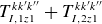 $T_{I,{1}{z}{1}}^{{k}{k^{\prime }}{k^{\prime \prime }}}+T_{I,{2}{z}{1}}^{{k}{k^{\prime }}{k^{\prime \prime }}}$
and
$T_{I,{1}{z}{1}}^{{k}{k^{\prime }}{k^{\prime \prime }}}+T_{I,{2}{z}{1}}^{{k}{k^{\prime }}{k^{\prime \prime }}}$
and $T_{I,{1}{z}{1}}^{{k^{\prime \prime }}{-k^{\prime }}{k(*)}}+T_{I,{2}{z}{1}}^{{k^{\prime \prime }}{-k^{\prime }}{k(*)}}$
are in general non-trivial and do not appear to reduce in a simple transparent manner algebraically. It can be shown in the collisionless limit that all second-order correlations of eigenmodes (
$T_{I,{1}{z}{1}}^{{k^{\prime \prime }}{-k^{\prime }}{k(*)}}+T_{I,{2}{z}{1}}^{{k^{\prime \prime }}{-k^{\prime }}{k(*)}}$
are in general non-trivial and do not appear to reduce in a simple transparent manner algebraically. It can be shown in the collisionless limit that all second-order correlations of eigenmodes ( $\beta 's$
) in this system will saturate under the MS conditions. In contrast, the asymmetric solution suggested by (5.21) only corresponds to
$\beta 's$
) in this system will saturate under the MS conditions. In contrast, the asymmetric solution suggested by (5.21) only corresponds to $\partial _t \langle v_z^2\rangle =0$
, but does not yield a steady state for the eigenmodes. We present the relevant saturation calculations for the eigenmodes in a subsequent work (Azelis et al. Reference Azelis, Terry, Sprott and Li2026) and also confirm observations of MS solutions in a numerical simulation of the system. As such, the remainder of this analysis is focused on the symmetric solutions suggested by the MS condition of (5.13) and (5.14), which are a subset of the general case. We proceed by considering the collisionless thermal flux.
$\partial _t \langle v_z^2\rangle =0$
, but does not yield a steady state for the eigenmodes. We present the relevant saturation calculations for the eigenmodes in a subsequent work (Azelis et al. Reference Azelis, Terry, Sprott and Li2026) and also confirm observations of MS solutions in a numerical simulation of the system. As such, the remainder of this analysis is focused on the symmetric solutions suggested by the MS condition of (5.13) and (5.14), which are a subset of the general case. We proceed by considering the collisionless thermal flux.
In the collisionless limit, the unstable/stable eigenvector expression of (2.5) becomes
 \begin{align} R_j = \frac {\omega _j(1+k_\perp ^2)-k_y}{ k_y \epsilon _n}, \end{align}
with imaginary part
 \begin{align} \mathrm{Im} R_j = \frac {\pm \gamma (1+k_\perp ^2)}{k_y \epsilon _n}. \end{align}
Therefore,
 \begin{align} \mathrm{Im} R_2 = - \mathrm{Im} R_1 \end{align}
and
 \begin{align} \mathrm{Im}(R_1 +R_2) = 0. \end{align}
The collisionless heat flux is then given by
 \begin{align} Q = -\sum _k k_y \mathrm{Im} R_1 \big( \langle \beta _{1}^{2} \rangle -\langle \beta _{2}^{2} \rangle \big) = \sum _k \frac {\gamma (1+k_\perp ^2)}{ \epsilon _n} \big( \langle \beta _{1}^{2} \rangle -\langle \beta _{2}^{2} \rangle \big), \end{align}
which after expanding the sum for the $3-\boldsymbol{k}$
system becomes
$3-\boldsymbol{k}$
system becomes
 \begin{align} Q = \frac {1}{\epsilon _n}\big[\gamma (1+k_y^2) \big( \langle \beta _{1}^{2} \rangle -\langle \beta _{2}^{2} \rangle \big) + \gamma ^{\prime \prime }(1+k_x^{{\prime }2} +k_y^2) \big( \langle \beta _{1}^{{\prime\prime}2} \rangle -\langle \beta _{2}^{{\prime\prime}2} \rangle \big)\big]. \end{align}
The terms in (5.27) clearly indicate that energy in an unstable mode corresponds to positive $Q$
and down-gradient transport, whereas the converse is true for energy in a stable mode. The MS condition of (5.13) and (5.14) then implies turbulence characterised by perfectly balanced up/down-gradient transport over each individual fluctuation length scale (
$Q$
and down-gradient transport, whereas the converse is true for energy in a stable mode. The MS condition of (5.13) and (5.14) then implies turbulence characterised by perfectly balanced up/down-gradient transport over each individual fluctuation length scale ( $k^{-1}$
), i.e. states of zero net transport despite a finite fluctuation level. This matches the limiting behaviour of the collisional thermal flux (5.8) for
$k^{-1}$
), i.e. states of zero net transport despite a finite fluctuation level. This matches the limiting behaviour of the collisional thermal flux (5.8) for $\nu \rightarrow 0$
. Remarkably, a saturated ZF with zero collisionality appears to suggest ideal confinement in the presence of the ITG instability, given this system. Interestingly, this is in contradiction with quasilinear theories of transport, which having been developed from
$\nu \rightarrow 0$
. Remarkably, a saturated ZF with zero collisionality appears to suggest ideal confinement in the presence of the ITG instability, given this system. Interestingly, this is in contradiction with quasilinear theories of transport, which having been developed from $Q \propto \gamma /k_\perp ^2$
with no explicit accounting for stable modes, predict a finite flux whenever an instability is present (Kotschenreuther et al. Reference Kotschenreuther, Dorland, Beer and Hammett1995; Jenko, Dannert & Angioni Reference Jenko, Dannert and Angioni2005). This result raises the question of whether quasilinear models, such as Pueschel et al. (Reference Pueschel, Faber, Citrin, Hegna, Terry and Hatch2016), can be adapted to account for stable mode damping.
$Q \propto \gamma /k_\perp ^2$
with no explicit accounting for stable modes, predict a finite flux whenever an instability is present (Kotschenreuther et al. Reference Kotschenreuther, Dorland, Beer and Hammett1995; Jenko, Dannert & Angioni Reference Jenko, Dannert and Angioni2005). This result raises the question of whether quasilinear models, such as Pueschel et al. (Reference Pueschel, Faber, Citrin, Hegna, Terry and Hatch2016), can be adapted to account for stable mode damping.
The result $Q=0$
for
$Q=0$
for $\nu =0$
can be predicted without explicit consideration of ZF dynamics or the eigenmode decomposition utilised herein. One way to demonstrate this is by multiplying (2.2) by
$\nu =0$
can be predicted without explicit consideration of ZF dynamics or the eigenmode decomposition utilised herein. One way to demonstrate this is by multiplying (2.2) by $\phi _k^*$
and performing a sum over all
$\phi _k^*$
and performing a sum over all $\boldsymbol{k}$
to produce the expression
$\boldsymbol{k}$
to produce the expression
 \begin{align} \sum _{\boldsymbol{k}} [\delta (k_y)+k_\perp ^2]\frac {\partial |\phi _k|^2}{\partial t} - \epsilon _n Q + \sum _{\boldsymbol{k}} \nu k_\perp ^2 |\phi _k|^2 =0. \end{align}
We note that the nonlinearity vanishes via integration of an odd function over symmetric bounds. For $\nu =0$
, steady-state behaviour of
$\nu =0$
, steady-state behaviour of $|\phi _k|^2$
corresponds to
$|\phi _k|^2$
corresponds to $Q=0$
, and this conclusion is reached without the lengthy calculations presented herein. However, when presented in this context, the property
$Q=0$
, and this conclusion is reached without the lengthy calculations presented herein. However, when presented in this context, the property $Q=0$
merely takes the form of a constraint imposed upon the motions of the fluid, with little indication of the statistical properties of said motions or any significant phenomenology in terms of the fields being modelled. In the absence of the eigenmode decomposition, the constraint simply suggests dynamics that on average satisfy
$Q=0$
merely takes the form of a constraint imposed upon the motions of the fluid, with little indication of the statistical properties of said motions or any significant phenomenology in terms of the fields being modelled. In the absence of the eigenmode decomposition, the constraint simply suggests dynamics that on average satisfy
 \begin{align} \sum _k k_y \mathrm{Im} \langle \phi _{-k}p_k\rangle = 0. \end{align}
While this does indeed suggest on average that the overall thermal energy being transported across all fluctuation length scales in the $+\hat {\boldsymbol{x}}$
is cancelled by fluxes in the
$+\hat {\boldsymbol{x}}$
is cancelled by fluxes in the $-\hat {\boldsymbol{x}}$
, it is not clear at all how the system achieves such a state and provides minimal description of the governing physics. Furthermore, there is no indication of whether the system has any particular preference for how the zero sum is achieved. It is an ambiguous linear combination of cross-correlations for which there are infinitely many possible
$-\hat {\boldsymbol{x}}$
, it is not clear at all how the system achieves such a state and provides minimal description of the governing physics. Furthermore, there is no indication of whether the system has any particular preference for how the zero sum is achieved. It is an ambiguous linear combination of cross-correlations for which there are infinitely many possible $\phi _k$
and
$\phi _k$
and $p_k$
products that may satisfy it. Our result suggests that the system has a particular preference for equipartition of energy between eigenmodes at each fluctuation length scale
$p_k$
products that may satisfy it. Our result suggests that the system has a particular preference for equipartition of energy between eigenmodes at each fluctuation length scale $k^{-1}$
and demonstrates this within the context of the underlying turbulent saturation theory physics.
$k^{-1}$
and demonstrates this within the context of the underlying turbulent saturation theory physics.
6. Generalisation to the many $-\boldsymbol{k}$
problem
$-\boldsymbol{k}$
problem

In can be shown that the ZF of the many $-\boldsymbol{k}$
system described by (2.19)–(2.21) has a WKE at lowest non-trivial order in perturbation described by
$-\boldsymbol{k}$
system described by (2.19)–(2.21) has a WKE at lowest non-trivial order in perturbation described by
 \begin{align} \partial _t \langle v_z^{2}\rangle = -2\left [\nu - K(k) \right ]\langle v_z^{2}\rangle , \end{align}
where
 \begin{align} K(k) = \mathrm{Re} \biggl [\sum _{k^{\prime }} C_{zmn}^{({k},{k^{\prime }},{k^{\prime \prime }})} \biggl (&\frac {C_{mzp}^{({k^{\prime }},{k},{-k^{\prime \prime }})}\langle \beta _{p}^{{\prime\prime}*}\beta _{n}^{\prime\prime}\rangle }{\mathrm{i}(\omega _{m}^{{\prime } }-\omega _{z}^{}+\omega _{p}^{{\prime\prime}*})} +\frac {C_{mqz}^{({k^{\prime }},{-k^{\prime \prime }},{k})}\langle \beta _{q}^{{\prime\prime}*}\beta _{n}^{\prime\prime}\rangle }{\mathrm{i}(\omega _{m}^{{\prime } }+\omega _{q}^{{\prime\prime}*}-\omega _{z}^{})} \nonumber \\[4pt] &+ \frac {C_{nzp}^{({k^{\prime \prime }},{k},{-k^{\prime }})}\langle \beta _{p}^{{\prime }*}\beta _{m}^{{\prime } }\rangle }{\mathrm{i}(\omega _{n}^{\prime\prime}-\omega _{z}^{}+\omega _{p}^{{\prime }*})} +\frac {C_{nqz}^{({k^{\prime \prime }},{-k^{\prime }},{k})}\langle \beta _{q}^{{\prime }*}\beta _{m}^{{\prime } }\rangle }{\mathrm{i}(\omega _{n}^{\prime\prime}+\omega _{q}^{{\prime }*}-\omega _{z}^{})}\biggl ) \biggl ]. \end{align}
The solution is given by
 \begin{align} \langle v_z^{2}\rangle (k_x,t) = \langle v_z^{2}\rangle _{t=0} \textrm {e}^{-2[\nu - K(k)]t}. \end{align}
The calculation is similar to Appendix A but with several subtle differences. One in particular is associated with the fourth-order moments not automatically being closed, but this is handled by the perturbation theory (Malfliet Reference Malfliet1972) with ease. This derivation is outside the scope of the current paper and would require many more pages, hence, it is omitted. However, it is not hard to show the result by following the methods of Malfliet (Reference Malfliet1972) in combination with the gyrokinetics-informed perturbative ordering scheme of Terry et al. (Reference Terry, Faber, Hegna, Mirnov, Pueschel and Whelan2018).
Striking similarities are observed between $K$
and
$K$
and $\kappa$
, with the key differences being the sum
$\kappa$
, with the key differences being the sum $\text{d}\boldsymbol{k}'$
over fluctuations and the fact that there are four terms instead of two. Nearly identical analysis can show nonetheless that the WKE of (6.1) also exhibits MS solutions in the collisionless limit with comparable up/down-gradient transport cancellations leading to the same saturation phenomenology. This is not surprising as the systems of equations (2.19)–(2.21) and (2.25)–(2.27) are akin, and it has previously been demonstrated that the
$\text{d}\boldsymbol{k}'$
over fluctuations and the fact that there are four terms instead of two. Nearly identical analysis can show nonetheless that the WKE of (6.1) also exhibits MS solutions in the collisionless limit with comparable up/down-gradient transport cancellations leading to the same saturation phenomenology. This is not surprising as the systems of equations (2.19)–(2.21) and (2.25)–(2.27) are akin, and it has previously been demonstrated that the $3-\boldsymbol{k}$
system reproduces similar saturation physics as the many
$3-\boldsymbol{k}$
system reproduces similar saturation physics as the many $-\boldsymbol{k}$
system (Li & Terry Reference Li and Terry2022). The primary differences between the systems arise from the vastly increased number of dynamical degrees of freedom in the many
$-\boldsymbol{k}$
system (Li & Terry Reference Li and Terry2022). The primary differences between the systems arise from the vastly increased number of dynamical degrees of freedom in the many $-\boldsymbol{k}$
system. In particular, this system does not impose any explicit constraints on the kurtosis. Moreover, the absence of wavenumber truncation enables the development of a full turbulence cascade, though its character differs from the standard forward-Kolmogorov picture in the collisionless limit.
$-\boldsymbol{k}$
system. In particular, this system does not impose any explicit constraints on the kurtosis. Moreover, the absence of wavenumber truncation enables the development of a full turbulence cascade, though its character differs from the standard forward-Kolmogorov picture in the collisionless limit.
For $\chi = \nu = 0$
, the imaginary portion
$\chi = \nu = 0$
, the imaginary portion $\gamma _j$
of the complex mode frequency (2.6) is finite and positive within a contour in the
$\gamma _j$
of the complex mode frequency (2.6) is finite and positive within a contour in the $k_xk_y$
plane satisfying (2.8). Outside this contour,
$k_xk_y$
plane satisfying (2.8). Outside this contour, $\gamma _j=0$
and all modes are marginally stable, exhibiting only oscillatory behaviour. (In contrast, for finite collisionality,
$\gamma _j=0$
and all modes are marginally stable, exhibiting only oscillatory behaviour. (In contrast, for finite collisionality, $\gamma _j$
remains finite but asymptotically decays to zero with increasing wavenumber, i.e.
$\gamma _j$
remains finite but asymptotically decays to zero with increasing wavenumber, i.e. $\lim _{k\rightarrow \infty } \gamma _j = 0$
.) Hence, in the collisionless limit, only a fraction of the modes are capable of either injecting or removing energy from the system, and this behaviour only occurs in a bounded and connected region of the Fourier domain. Saturation of the full wavenumber system therefore requires a mechanism by which energy, nonlinearly transferred via forward cascade to wavenumbers beyond the contour in (2.8), is eventually returned to the stable modes within that contour, where it can then be removed.
$\lim _{k\rightarrow \infty } \gamma _j = 0$
.) Hence, in the collisionless limit, only a fraction of the modes are capable of either injecting or removing energy from the system, and this behaviour only occurs in a bounded and connected region of the Fourier domain. Saturation of the full wavenumber system therefore requires a mechanism by which energy, nonlinearly transferred via forward cascade to wavenumbers beyond the contour in (2.8), is eventually returned to the stable modes within that contour, where it can then be removed.
It has been observed that the plasma wave echo phenomenon (Gould, O’Neil & Malmberg Reference Gould, O’Neil and Malmberg1967; Malmberg et al. Reference Malmberg, Wharton, Gould and O’Neil1968) can inversely cascade energy from high to low wavenumbers in long-wavelength electrostatic turbulence in magnetised, weakly collisional plasmas, including (but not limited to) ITG drift-wave turbulence (Schekochihin et al. Reference Schekochihin, Parker, Highcock, Dellar, Dorland and Hammett2016). It has also been demonstrated that in trapped electron mode turbulence, where saturation occurs via energy transfer to stable modes (Terry et al. Reference Terry, Gatto and Baver2002), wavenumber anisotropy gives rise to inverse energy transfer that condenses onto zonal modes (Terry Reference Terry2004). However, a full investigation of energy-transfer mechanisms in the collisionless many $-\boldsymbol{k}$
system lies beyond the scope of this study and is left for future work.
$-\boldsymbol{k}$
system lies beyond the scope of this study and is left for future work.
7. Conclusions
A weak-turbulence closure method (Malfliet Reference Malfliet1972) was used in conjunction with a reduced fluid model for ITG-driven turbulence (Horton et al. Reference Horton, Choi and Tang1981, Reference Horton, Hong and Tang1988; Terry et al. Reference Terry, Faber, Hegna, Mirnov, Pueschel and Whelan2018; Li & Terry Reference Li and Terry2022) to calculate a ZF WKE. The equation, in particular its nonlinear time-evolution operator, was then analysed in the collisionless limit to look for stationary solutions and ZF spectral saturation mechanisms. Solutions were found suggesting collisionless ZF saturation characterised by symmetric up/down-gradient thermal energy transport, and ideal confinement despite the ITG instability. For systems with small but finite collisionality, these findings suggest that ITG-driven turbulence exhibits progressively more equal partitioning of energy between counter-transporting fluctuations at each characteristic length scale as collisionality is reduced, approaching exact equipartition in the collisionless limit.
This result was found from the MS condition of (5.13) and (5.14), which suggest that saturation occurs for $\langle \beta _{1}^{2} \rangle =\langle \beta _{2}^{2} \rangle$
and
$\langle \beta _{1}^{2} \rangle =\langle \beta _{2}^{2} \rangle$
and $\langle \beta _{1}^{{\prime\prime}2} \rangle =\langle \beta _{2}^{{\prime\prime}2} \rangle$
. The ZF is the primary catalyst of resonant energy transfer from the unstable mode to the stable mode in this model, so it appears reasonable that if there exists the opportunity for it to give as much as it can receive with equal rate and proportion, it will neither grow nor decay. In the collisionless limit, the unstable growth rate is equal and opposite to the stable-mode damping rate. The linear instability physics, which adds or removes energy, are already balanced, so if at each
$\langle \beta _{1}^{{\prime\prime}2} \rangle =\langle \beta _{2}^{{\prime\prime}2} \rangle$
. The ZF is the primary catalyst of resonant energy transfer from the unstable mode to the stable mode in this model, so it appears reasonable that if there exists the opportunity for it to give as much as it can receive with equal rate and proportion, it will neither grow nor decay. In the collisionless limit, the unstable growth rate is equal and opposite to the stable-mode damping rate. The linear instability physics, which adds or removes energy, are already balanced, so if at each $\boldsymbol{k}$
the energy is equipartitioned between the stable and unstable mode, the nonlinearity connecting the two through the ZF should be as well. This is also suggested graphically by figure 1. The ZF (yellow arrows) is the mediator for transfer between the system’s sources (unstable modes) and sinks (stable modes). It makes sense that it should remain relatively energetically steady when what is flowing into it indirectly from the gradient is equal to what flows out and back to
$\boldsymbol{k}$
the energy is equipartitioned between the stable and unstable mode, the nonlinearity connecting the two through the ZF should be as well. This is also suggested graphically by figure 1. The ZF (yellow arrows) is the mediator for transfer between the system’s sources (unstable modes) and sinks (stable modes). It makes sense that it should remain relatively energetically steady when what is flowing into it indirectly from the gradient is equal to what flows out and back to $\eta$
. These notions then correspond to states in which energy is neither escaping nor accumulating in the solution space.
$\eta$
. These notions then correspond to states in which energy is neither escaping nor accumulating in the solution space.
Phenomenologically, this result then begs the question of whether minimising collisionality can be advantageous for mitigating transport due to the ITG instability. Instead of trying to prevent heat from escaping, perhaps with something akin to a transport barrier, can an ultra low-collisionality ( $\nu =0$
is an impossible idealisation) plasma be prepared or driven in such a way that the heat moving down gradient is nearly balanced by what is moving in the opposite direction? It had previously been found by Hatch et al. (Reference Hatch, Jenko, Bañón Navarro and Bratanov2013) that decreasing collisionality results in increased amounts of energy going into the cascade, as opposed to stable modes at the same
$\nu =0$
is an impossible idealisation) plasma be prepared or driven in such a way that the heat moving down gradient is nearly balanced by what is moving in the opposite direction? It had previously been found by Hatch et al. (Reference Hatch, Jenko, Bañón Navarro and Bratanov2013) that decreasing collisionality results in increased amounts of energy going into the cascade, as opposed to stable modes at the same $k$
. This would appear to suggest that stable modes are only of importance when collisionality is high. However, that paper was restricted to measurement of the role of low-
$k$
. This would appear to suggest that stable modes are only of importance when collisionality is high. However, that paper was restricted to measurement of the role of low- $k$
stable modes on collisional dissipation. It has since been better appreciated that stable modes put energy back into the instability-driving gradient through a process that reverses the instability process and does not contribute to entropy increase. This was not measured in Hatch. This process functions at zero collisionality and is the basis of the effects described in this paper. It is the dominant stable-mode effect in high-Reynolds-number hydrodynamic (Tripathi et al. Reference Tripathi, Terry, Fraser, Zweibel and Pueschel2023b
) and magnetohydrodynamic Kelvin–Helmholtz-driven turbulence (Fraser et al. Reference Fraser, Terry, Zweibel, Pueschel and Schroeder2021; Tripathi et al. Reference Tripathi, Fraser, Terry, Zweibel and Pueschel2022b
) and in low to zero collisionality fluid ITG turbulence. While this process arises in gyrokinetics, the gyrokinetic case has received less attention than fluid systems.
$k$
stable modes on collisional dissipation. It has since been better appreciated that stable modes put energy back into the instability-driving gradient through a process that reverses the instability process and does not contribute to entropy increase. This was not measured in Hatch. This process functions at zero collisionality and is the basis of the effects described in this paper. It is the dominant stable-mode effect in high-Reynolds-number hydrodynamic (Tripathi et al. Reference Tripathi, Terry, Fraser, Zweibel and Pueschel2023b
) and magnetohydrodynamic Kelvin–Helmholtz-driven turbulence (Fraser et al. Reference Fraser, Terry, Zweibel, Pueschel and Schroeder2021; Tripathi et al. Reference Tripathi, Fraser, Terry, Zweibel and Pueschel2022b
) and in low to zero collisionality fluid ITG turbulence. While this process arises in gyrokinetics, the gyrokinetic case has received less attention than fluid systems.
This work was Part I of a two-part series on collisionless ITG-driven turbulence. In Part II we will present weak-turbulence closure calculations for $\langle \beta _{j}^{2} \rangle$
and
$\langle \beta _{j}^{2} \rangle$
and $\langle \beta _{j}^{{\prime\prime}2} \rangle$
that are analysed through the lens of dynamical systems theory. Furthermore, we will investigate the phase-space behaviour of the aforementioned modes and their predilection for MS. This work will be complemented by results from numerical simulations of the
$\langle \beta _{j}^{{\prime\prime}2} \rangle$
that are analysed through the lens of dynamical systems theory. Furthermore, we will investigate the phase-space behaviour of the aforementioned modes and their predilection for MS. This work will be complemented by results from numerical simulations of the $3-\boldsymbol{k}$
system. Beyond this, it may be of interest to consider more closely the many-
$3-\boldsymbol{k}$
system. Beyond this, it may be of interest to consider more closely the many- $\boldsymbol{k}$
system and compare the results with simulations of gyrokinetics.
$\boldsymbol{k}$
system and compare the results with simulations of gyrokinetics.
There are hints that solutions of the collisionless system are appreciably more sensitive to initial conditions than the collisional system. This may be of fundamental importance when performing simulations and subsequent mathematical analysis. Many infinite-dimensional dynamical systems with diffusion or dissipation possess an absorbing set, which traps all trajectories in a bounded region of phase space. In essence, dissipative terms can damp out high- $\boldsymbol{k}$
modes, while nonlinearities transfer energy among the modes. The balancing between these effects can produce finite-dimensional asymptotic dynamics. For instance, it is well known that the two-dimensional Navier–Stokes equations possess a finite-dimensional attractor (Hale Reference Hale1988; Temam Reference Temam1997; Foias et al. Reference Foias, Manley, Rosa and Temam2001). There exists the possibility that the reduced two-field fluid model system of (2.1) and (2.2) exhibits a fundamental change in its phase space in the limit
$\boldsymbol{k}$
modes, while nonlinearities transfer energy among the modes. The balancing between these effects can produce finite-dimensional asymptotic dynamics. For instance, it is well known that the two-dimensional Navier–Stokes equations possess a finite-dimensional attractor (Hale Reference Hale1988; Temam Reference Temam1997; Foias et al. Reference Foias, Manley, Rosa and Temam2001). There exists the possibility that the reduced two-field fluid model system of (2.1) and (2.2) exhibits a fundamental change in its phase space in the limit $\nu = 0$
that is analogous to the difference between parabolic and hyperbolic second-order PDEs (for instance, consider the difference in solutions to Burger’s equation and its inviscid counterpart or the Navier–Stokes equation and the Euler’s equation). However, the distinction and necessary analysis to make such a strong conclusion is non-trivial due to said equations being third order. These topics will be discussed in a future work.
$\nu = 0$
that is analogous to the difference between parabolic and hyperbolic second-order PDEs (for instance, consider the difference in solutions to Burger’s equation and its inviscid counterpart or the Navier–Stokes equation and the Euler’s equation). However, the distinction and necessary analysis to make such a strong conclusion is non-trivial due to said equations being third order. These topics will be discussed in a future work.
Acknowledgements
AAA thanks Felix Parra for mentioning plasma wave echoes in conversation.
Editor Alex Schekochihin thanks the referees for their advice in evaluating this article.
Funding
This work was supported by the US DOE grant DE-FG02-89ER53291.
Declaration of interests
The authors report no conflict of interest.
Appendix A. Weak-turbulence closure of ZF energy spectrum
In this appendix, a weak-turbulence closure technique (Malfliet Reference Malfliet1972) for instability-driven systems is employed to calculate a ZF WKE. This WKE characterises the manner in which the energy of the ZF $v_z'$
will fluctuate with time according to both linear and nonlinear dynamics. The closure method demonstrated herein is different from those for dispersive systems without instability (see, for instance, Benney & Newell (Reference Benney and Newell1969), Zakharov et al. (Reference Zakharov, L’Vov and Falkovich1992), Nazarenko (Reference Nazarenko2011), Galtier (Reference Galtier2023a
,
Reference Galtierb
) and Azelis et al. (Reference Azelis, Perez and Bourouaine2024) for thorough tutorials on such matters). A key difference is the need to exercise caution because the linear eigenmodes and correlation expressions in this work contain real exponentials, which are not in
$v_z'$
will fluctuate with time according to both linear and nonlinear dynamics. The closure method demonstrated herein is different from those for dispersive systems without instability (see, for instance, Benney & Newell (Reference Benney and Newell1969), Zakharov et al. (Reference Zakharov, L’Vov and Falkovich1992), Nazarenko (Reference Nazarenko2011), Galtier (Reference Galtier2023a
,
Reference Galtierb
) and Azelis et al. (Reference Azelis, Perez and Bourouaine2024) for thorough tutorials on such matters). A key difference is the need to exercise caution because the linear eigenmodes and correlation expressions in this work contain real exponentials, which are not in $L^1$
, bringing into question the boundedness of various functions in a rigorous sense, and applicability of certain notions of functional analysis such as the Riemann–Lebesgue lemma (Benney & Newell Reference Benney and Newell1969; Davies Reference Davies2002). See Appendix D for further discussion on these matters.
$L^1$
, bringing into question the boundedness of various functions in a rigorous sense, and applicability of certain notions of functional analysis such as the Riemann–Lebesgue lemma (Benney & Newell Reference Benney and Newell1969; Davies Reference Davies2002). See Appendix D for further discussion on these matters.
A.1. Construction of the moment hierarchy
The starting point of the calculation is a set of equations that describe the manner in which amplitudes in the 3 $-\boldsymbol{k}$
system evolve over time according to
$-\boldsymbol{k}$
system evolve over time according to
 \begin{align} \dot {\beta _l} +\mathrm{i}\omega _l \beta _l & = C_{lzn}^{({k},{k^{\prime }},{k^{\prime \prime }})} v_z^{{\prime } }\beta _{n}^{\prime\prime},\\[-10pt]\nonumber \end{align}
 \begin{align} \dot {\beta _{l}^{\prime\prime}} +\mathrm{i}\omega _{l}^{\prime\prime} \beta _{l}^{\prime\prime} & = C_{lzn}^{({k^{\prime \prime }},{-k^{\prime }},{k})} v_z^{{\prime }*}\beta _{n}^{},\\[-10pt]\nonumber \end{align}
 \begin{align} \dot {v_z^{{\prime }}} + \nu v_z^{{\prime }} & = C_{zmn}^{({k^{\prime }},{k},{-k^{\prime \prime }})}\beta _{m}^{}\beta _{n}^{{\prime\prime}*}. \end{align}
A change of variables of the form
 \begin{align} \beta _{l}^{} & = \tilde {\beta }_{l}^{}\textrm {e}^{-\mathrm{i}\omega _{l}^{}t} ,\\[-10pt]\nonumber \end{align}
 \begin{align} v_z^{{\prime }} & = \tilde {v}_z^{{\prime }}\textrm {e}^{-\mathrm{i}\omega _z t} \end{align}
is introduced with the intent of isolating the linear and nonlinear portions of modal amplitude time evolution, in which the linear eigenvalues are written compactly as
 \begin{align} \omega _{l}^{} & = \varpi _l \pm \mathrm{i} \gamma _{l} ,\\[-10pt]\nonumber \end{align}
 \begin{align} \omega _z & = -\mathrm{i} \nu . \end{align}
The ZF spectra in the two different representations relate to one another as
 \begin{align} \langle v_z^{{\prime }2} \rangle = v_z^{{\prime }}v_z^{{\prime }*} = \tilde {v}_z^{{\prime }}\textrm {e}^{-\mathrm{i}\omega _z t} \tilde {v}_z^{{\prime }*}\textrm {e}^{\mathrm{i}\omega _z^* t} = \langle \tilde {v}_z^{{\prime }2} \rangle \textrm {e}^{-2\nu t}. \end{align}
Equations (A1)–(A3) for modal amplitude time evolution become
 \begin{align} \partial _t\tilde {\beta }_{l}^{} &= C_{lzn}^{({k},{k^{\prime }},{k^{\prime \prime }})} \tilde {v}_z^{{\prime } }\tilde {\beta }_{n}^{\prime\prime} \textrm {e}^{\mathrm{i}(\omega _{l}^{}-\omega _{z}^{}-\omega _{n}^{\prime\prime})t} ,\\[-10pt]\nonumber\end{align}
 \begin{align} \partial _t\tilde {\beta }_{l}^{\prime\prime} &= C_{lzn}^{({k^{\prime \prime }},{-k^{\prime }},{k})} \tilde {v}_z^{{\prime } *}\tilde {\beta }_{n}^{}\textrm {e}^{\mathrm{i}(\omega _{l}^{\prime\prime}+\omega _{z}^{*}-\omega _{n}^{})t} ,\\[-10pt]\nonumber\end{align}
 \begin{align} \partial _t\tilde {v}_z^{{\prime }} &= C_{zmn}^{({k^{\prime }},{k},{-k^{\prime \prime }})}\tilde {\beta }_{m}^{}\tilde {\beta }_{n}^{{\prime\prime}*}\textrm {e}^{\mathrm{i}(\omega _z - \omega _{i}^{} +\omega _{j}^{{\prime\prime}*})t}, \end{align}
which gives the quantities with tildes the meaning of only evolving due to nonlinear interactions with other fluctuations. Then, it is not hard to show that the ZF energy evolves in time according to
 \begin{align} \partial _t \langle \tilde {v}_z^{{\prime }2} \rangle = 2 \mathrm{Re}\big( C_{zij}^{({k^{\prime }},{k},{-k^{\prime \prime }})}\big\langle \tilde {v}_z^{{\prime } *}\tilde {\beta }_{i}^{}\tilde {\beta }_{j}^{{\prime\prime}*} \big\rangle \textrm {e}^{\mathrm{i}(\omega _z - \omega _{i}^{} +\omega _{j}^{{\prime\prime}*})t} \big). \end{align}
A closure problem is encountered and an expression is required for the third-order moment $\langle \tilde {v}_z^{{\prime } *}\tilde {\beta }_{i}^{}\tilde {\beta }_{j}^{{\prime\prime}*} \rangle$
. For the
$\langle \tilde {v}_z^{{\prime } *}\tilde {\beta }_{i}^{}\tilde {\beta }_{j}^{{\prime\prime}*} \rangle$
. For the $3-\boldsymbol{k}$
system, the fourth-order moments encountered automatically close, e.g.
$3-\boldsymbol{k}$
system, the fourth-order moments encountered automatically close, e.g.
 \begin{align} \big\langle \big(\tilde {v}_z^{{\prime }*}\tilde {\beta }_{j}^{{\prime\prime}*}\big)\partial _t \tilde {\beta }_{i}^{} \big\rangle \propto \big\langle \big(\tilde {v}_z^{{\prime }*}\tilde {\beta }_{j}^{{\prime\prime}*}\big) \tilde {v}_z^{{\prime }}\tilde {\beta }_{m}^{\prime\prime} \big\rangle =\big\langle \tilde {v}_z^{{\prime }2} \tilde {\beta }_{j}^{{\prime\prime}*}\tilde {\beta }_{m}^{\prime\prime} \big\rangle = \langle \tilde {v}_z^{{\prime }2} \rangle \big\langle \tilde {\beta }_{j}^{{\prime\prime}*}\tilde {\beta }_{m}^{\prime\prime} \big\rangle . \end{align}
This is because the second-order correlations of $\tilde {v}_z^{{\prime }}=\tilde {v}_z(k_x',0)$
with
$\tilde {v}_z^{{\prime }}=\tilde {v}_z(k_x',0)$
with $\beta _{j}^{\prime\prime}=\beta _j(k_x^{\prime \prime },k_y^{\prime \prime })$
(or their complex conjugates) exhibit statistical independence of the form
$\beta _{j}^{\prime\prime}=\beta _j(k_x^{\prime \prime },k_y^{\prime \prime })$
(or their complex conjugates) exhibit statistical independence of the form
 \begin{align} \big\langle \tilde {v}_z^{{\prime }} \tilde {\beta }_{j}^{\prime\prime} \big\rangle = \big\langle \tilde {v}_z^{{\prime }} \tilde {\beta }_{j}^{\prime\prime} \big\rangle \delta (\boldsymbol{k}'+\boldsymbol{k}^{\prime \prime }) = 0, \end{align}
under the assumption of spatially homogeneous turbulence (Batchelor Reference Batchelor1953) built into the reduced two-field fluid model and exploited by the closure method (Malfliet Reference Malfliet1972). Equivalently (to the implication of (A13)), the fourth-order cumulant for the $3-\boldsymbol{k}$
system is identically zero. Note that the property of spatial homogeneity (frequently exploited in weak-turbulence closures; see, e.g. Benney & Newell Reference Benney and Newell1969) is different from the obvious fact that these fluctuations evolve due to one another at any given moment in time (so as not to conflate with what is meant by `statistical independence’), and is a general statement regarding statistical long time averaging as well as the nature of the turbulent fluid’s spatial distribution, not necessarily its explicit instantaneous dynamical behaviour.
$3-\boldsymbol{k}$
system is identically zero. Note that the property of spatial homogeneity (frequently exploited in weak-turbulence closures; see, e.g. Benney & Newell Reference Benney and Newell1969) is different from the obvious fact that these fluctuations evolve due to one another at any given moment in time (so as not to conflate with what is meant by `statistical independence’), and is a general statement regarding statistical long time averaging as well as the nature of the turbulent fluid’s spatial distribution, not necessarily its explicit instantaneous dynamical behaviour.
In general, every correlation of fluctuations in this work has an implied Dirac delta function attached, which is always understood to be present, but omitted in the interest of brevity. For instance, the third-order correlation $\langle \tilde {v}_z^{{\prime } *}\tilde {\beta }_{i}^{}\tilde {\beta }_{j}^{{\prime\prime}*} \rangle$
of ZF spectral evolution (A12) has an implied
$\langle \tilde {v}_z^{{\prime } *}\tilde {\beta }_{i}^{}\tilde {\beta }_{j}^{{\prime\prime}*} \rangle$
of ZF spectral evolution (A12) has an implied $\delta (\boldsymbol{k}-\boldsymbol{k}'-\boldsymbol{k}^{\prime \prime })$
associated with it. Mathematically, these delta functions arise due to Fourier transforms of nonlinearities, while physically, they correspond to the statistics of
$\delta (\boldsymbol{k}-\boldsymbol{k}'-\boldsymbol{k}^{\prime \prime })$
associated with it. Mathematically, these delta functions arise due to Fourier transforms of nonlinearities, while physically, they correspond to the statistics of $n$
-point spatial correlations (the real-space equivalent of the correlations of Fourier amplitudes observed herein) only depending on relative separations between the locations at which the fields are being evaluated, not the particular positions in the flow. For example, for a spatially homogeneous system, the two-point correlation
$n$
-point spatial correlations (the real-space equivalent of the correlations of Fourier amplitudes observed herein) only depending on relative separations between the locations at which the fields are being evaluated, not the particular positions in the flow. For example, for a spatially homogeneous system, the two-point correlation $F(\boldsymbol{x},\boldsymbol{r})$
of some field
$F(\boldsymbol{x},\boldsymbol{r})$
of some field $f(\boldsymbol{x})$
with itself,
$f(\boldsymbol{x})$
with itself,
 \begin{align} F(\boldsymbol{x},\boldsymbol{r}) = \langle f(\boldsymbol{x}) f(\boldsymbol{x}+\boldsymbol{r})\rangle , \end{align}
only depends on separation $\boldsymbol{r}$
, such that
$\boldsymbol{r}$
, such that $F=F(\boldsymbol{r})$
. The correlation
$F=F(\boldsymbol{r})$
. The correlation $F(\boldsymbol{r})$
may be written in terms of Fourier transforms as
$F(\boldsymbol{r})$
may be written in terms of Fourier transforms as
 \begin{align} F(\boldsymbol{r}) = \langle f(\boldsymbol{x}) f(\boldsymbol{x}+\boldsymbol{r})\rangle &= \int \text{d}\boldsymbol{k} \text{d}\boldsymbol{k}' \langle f(\boldsymbol{k}) f(\boldsymbol{k}') \rangle \textrm {e}^{\mathrm{i}\boldsymbol{k}\boldsymbol{\cdot }\boldsymbol{x}} \textrm {e}^{\mathrm{i} \boldsymbol{k}'\boldsymbol{\cdot }(\boldsymbol{x}+\boldsymbol{r})} \nonumber \\ &= \int \text{d}\boldsymbol{k} \text{d}\boldsymbol{k}' \langle f(\boldsymbol{k}) f(\boldsymbol{k}') \rangle \textrm {e}^{\mathrm{i}(\boldsymbol{k}+\boldsymbol{k}')\boldsymbol{\cdot }\boldsymbol{x}} \textrm {e}^{\mathrm{i} \boldsymbol{k}'\boldsymbol{\cdot }\boldsymbol{r}}, \end{align}
but if $F(\boldsymbol{r})$
is independent of
$F(\boldsymbol{r})$
is independent of $\boldsymbol{x}$
, the right-hand integral must follow suit and it is required that
$\boldsymbol{x}$
, the right-hand integral must follow suit and it is required that $\boldsymbol{k}+\boldsymbol{k}'=0$
. Therefore, the correlation
$\boldsymbol{k}+\boldsymbol{k}'=0$
. Therefore, the correlation $F(\boldsymbol{r})$
is
$F(\boldsymbol{r})$
is
 \begin{align} F(\boldsymbol{r})= \int \text{d}\boldsymbol{k} \text{d}\boldsymbol{k}' \langle f(\boldsymbol{k}) f(\boldsymbol{k}') \rangle \textrm {e}^{\mathrm{i}(\boldsymbol{k}+\boldsymbol{k}')\boldsymbol{\cdot }\boldsymbol{x}} \textrm {e}^{\mathrm{i} \boldsymbol{k}'\boldsymbol{\cdot }\boldsymbol{r}}\delta (\boldsymbol{k}+\boldsymbol{k}') = \int \text{d}\boldsymbol{k} \langle f(\boldsymbol{k}) f({-}\boldsymbol{k}) \rangle \textrm {e}^{-\mathrm{i} \boldsymbol{k}\boldsymbol{\cdot }\boldsymbol{r}}. \end{align}
The above result readily generalises to any moment or cumulant presented herein, and is the reasoning for the lack of correlation between $\tilde {v}_z^{{\prime }}$
and
$\tilde {v}_z^{{\prime }}$
and $\tilde {\beta }_{j}^{\prime\prime}$
described by (A14). Furthermore, if
$\tilde {\beta }_{j}^{\prime\prime}$
described by (A14). Furthermore, if $\boldsymbol{k}' = \boldsymbol{k}^{\prime \prime }$
were allowed to be true then this would imply that eigenmode
$\boldsymbol{k}' = \boldsymbol{k}^{\prime \prime }$
were allowed to be true then this would imply that eigenmode $\beta _{j}^{\prime\prime}$
is a ZF such that
$\beta _{j}^{\prime\prime}$
is a ZF such that $\beta _{j}^{\prime\prime}=\beta _{j}^{\prime\prime}\delta (k_y^{\prime \prime })=\tilde {v}_z^{\prime\prime}$
. However, this leads to a contradiction arising in the ZF spectral evolution equation (A12) of the form
$\beta _{j}^{\prime\prime}=\beta _{j}^{\prime\prime}\delta (k_y^{\prime \prime })=\tilde {v}_z^{\prime\prime}$
. However, this leads to a contradiction arising in the ZF spectral evolution equation (A12) of the form $C_{zij}^{({k^{\prime }},{k},{-k^{\prime \prime }})}\delta (k_y^{\prime \prime }) = 0$
, and such an interaction therefore never occurs.
$C_{zij}^{({k^{\prime }},{k},{-k^{\prime \prime }})}\delta (k_y^{\prime \prime }) = 0$
, and such an interaction therefore never occurs.
The fourth-order moment reduction allotted by (A13) suggests an interesting detail, namely that the fluctuation probability distribution function of the $3-\boldsymbol{k}$
system of equations always has the equivalent of what is considered a ‘Gaussian’-kurtosis value. This contrasts with the less restrictive many
$3-\boldsymbol{k}$
system of equations always has the equivalent of what is considered a ‘Gaussian’-kurtosis value. This contrasts with the less restrictive many $-\boldsymbol{k}$
system of (2.19)–(2.21), where the fourth-order cumulant is generally non-zero. While this constraint on the phase-space statistics is interesting, it is not the focus of this work. Weak-turbulence closure calculations carried to the lowest non-trivial order in perturbation usually discard or neglect the fourth-order cumulant for one reason or another.
$-\boldsymbol{k}$
system of (2.19)–(2.21), where the fourth-order cumulant is generally non-zero. While this constraint on the phase-space statistics is interesting, it is not the focus of this work. Weak-turbulence closure calculations carried to the lowest non-trivial order in perturbation usually discard or neglect the fourth-order cumulant for one reason or another.
Returning to the closure calculation, the third-order moment then evolves according to
 \begin{align} \partial _t \big\langle \tilde {v}_z^{{\prime }*} \tilde {\beta }_{i}^{}\tilde {\beta }_{j}^{{\prime\prime}*} \big\rangle = \langle \tilde {v}_z^{{\prime }2} \rangle \big(&C_{izm}^{({k},{k^{\prime }},{k^{\prime \prime }})}\big\langle \tilde {\beta }_{j}^{{\prime\prime}*} \tilde {\beta }_{m}^{\prime\prime} \big\rangle \textrm {e}^{\mathrm{i}(\omega _{i}^{} - \omega _z - \omega _{m}^{\prime\prime})t} \nonumber \\[5pt] &+ C_{jzm}^{({k^{\prime \prime }},{-k^{\prime }},{k})*}\big\langle \tilde {\beta }_{m}^{*}\tilde {\beta }_{i}^{} \big\rangle \textrm {e}^{-\mathrm{i}(\omega _{j}^{\prime\prime}-\omega _z-\omega _{m}^{})^*t}\big) \nonumber \\[5pt] &+C_{zmn}^{({k^{\prime }},{k},{-k^{\prime \prime }})*}\big\langle \tilde {\beta }_{m}^{*} \tilde {\beta }_{i}^{}\big\rangle \big\langle \tilde {\beta }_{j}^{{\prime\prime}*}\tilde {\beta }_{n}^{\prime\prime} \big\rangle \textrm {e}^{-\mathrm{i}(\omega _z - \omega _{m}^{} +\omega _{n}^{{\prime \prime}}{}^*)^*t}. \end{align}
A.2. Perturbation theory
The closed-form solution of the ZF spectral evolution equation (A12) necessitates an expression for the third-order moment $\langle \tilde {v}_z^{{\prime }*} \tilde {\beta }_{i}^{}\tilde {\beta }_{j}^{{\prime\prime}*} \rangle$
and not its time derivative. Hence, (A18) needs to be integrated. To achieve this, a perturbation theory (Malfliet Reference Malfliet1972) is introduced. Certain steps in the following analysis may seem trivial or unnecessary, but the goal of the present analysis is to carefully utilise the known technique, and not make new mathematical formalism or recklessly take shortcuts through the closure calculation. An attempt is made herein to contemporise the particular closure method (Malfliet Reference Malfliet1972) and provide some level of tutorial for instability-driven systems.
$\langle \tilde {v}_z^{{\prime }*} \tilde {\beta }_{i}^{}\tilde {\beta }_{j}^{{\prime\prime}*} \rangle$
and not its time derivative. Hence, (A18) needs to be integrated. To achieve this, a perturbation theory (Malfliet Reference Malfliet1972) is introduced. Certain steps in the following analysis may seem trivial or unnecessary, but the goal of the present analysis is to carefully utilise the known technique, and not make new mathematical formalism or recklessly take shortcuts through the closure calculation. An attempt is made herein to contemporise the particular closure method (Malfliet Reference Malfliet1972) and provide some level of tutorial for instability-driven systems.
The perturbative ordering scheme uses a weak-turbulence argument to make the assumptions
 \begin{align} \langle \tilde {\beta }_{l}^{2}\rangle , \langle \tilde {v}_z^{{\prime }2} \rangle = O(\epsilon ),\\[-10pt]\nonumber \end{align}
 \begin{align} \big\langle \tilde {\beta }_{1}^{*}\tilde {v}_z^{{\prime }} \tilde {\beta }_{n}^{\prime\prime}\big\rangle = O(\epsilon ^2) \end{align}
and
 \begin{align} \big\langle \tilde {\beta }_{1}^{*}\tilde {v}_z^{{\prime }}\tilde {v}_z^{\prime\prime\prime}\tilde {\beta }_{p}^{iv}\big\rangle = O(\epsilon ^3), \end{align}
i.e. the ordering of the functions in the statistical moment hierarchy follows a sequence of polynomials in $\epsilon$
of monotonic increasing order; the nth-order moment in statistics is
$\epsilon$
of monotonic increasing order; the nth-order moment in statistics is $O(\epsilon ^{n-1})$
in perturbation. Through the lens of
$O(\epsilon ^{n-1})$
in perturbation. Through the lens of $n$
-point spatial correlations this is in part a statement regarding the `randomness’ of the turbulence in real space; three points in the flow will be on average much less `similar’ to each other than two points, but far more than four. This notion dictates the manner in which a correlation will evolve over time due to others that drive it. Essentially, as will be shown, it amounts to an assumption of slowly varying functions, comparable to weak-turbulence methods used in dispersive systems (Benney & Newell Reference Benney and Newell1969), but executed slightly differently for the instability-driven system at hand.
$n$
-point spatial correlations this is in part a statement regarding the `randomness’ of the turbulence in real space; three points in the flow will be on average much less `similar’ to each other than two points, but far more than four. This notion dictates the manner in which a correlation will evolve over time due to others that drive it. Essentially, as will be shown, it amounts to an assumption of slowly varying functions, comparable to weak-turbulence methods used in dispersive systems (Benney & Newell Reference Benney and Newell1969), but executed slightly differently for the instability-driven system at hand.
When considering said systems, the weak-turbulence closure uses two separate perturbative expansions in spectral growth rate. One expansion is in terms of the overall time evolution $\partial _t \langle v_z^{{\prime }2}\rangle$
, which takes into account both linear and nonlinear dynamics, while the other only considers nonlinear influence as described by the function
$\partial _t \langle v_z^{{\prime }2}\rangle$
, which takes into account both linear and nonlinear dynamics, while the other only considers nonlinear influence as described by the function $\partial _t \langle \tilde {v}^{{\prime }2}_z\rangle$
. Then, the expansions are compared and matched (using the perturbation parameter
$\partial _t \langle \tilde {v}^{{\prime }2}_z\rangle$
. Then, the expansions are compared and matched (using the perturbation parameter $\epsilon$
) to obtain the WKE sought in this calculation. To begin, the spectral growth rate
$\epsilon$
) to obtain the WKE sought in this calculation. To begin, the spectral growth rate $ \partial _t \langle v_z^{{\prime }2} \rangle$
is expanded as
$ \partial _t \langle v_z^{{\prime }2} \rangle$
is expanded as
 \begin{align} \partial _t \langle v_z^{{\prime }2} \rangle = A_0 + \epsilon A_1 + \epsilon ^2 A_2 + \cdots\!, \end{align}
where $\epsilon \ll 1$
and the functions
$\epsilon \ll 1$
and the functions $A_i=O(1)$
are chosen according to the various terms encountered in the statistical moment hierarchy that governs ZF time evolution at each order in the perturbation. From (A19),
$A_i=O(1)$
are chosen according to the various terms encountered in the statistical moment hierarchy that governs ZF time evolution at each order in the perturbation. From (A19), $\langle v_z^{{\prime }2} \rangle =O(\epsilon )$
, and it is clear that
$\langle v_z^{{\prime }2} \rangle =O(\epsilon )$
, and it is clear that $A_0 = 0$
. Hence,
$A_0 = 0$
. Hence,
 \begin{align} \partial _t \langle v_z^{{\prime }2} \rangle = \epsilon A_1 + \epsilon ^2 A_2 + \cdots\! . \end{align}
Determination of the remaining functions $A_i$
requires a closed-form expression for
$A_i$
requires a closed-form expression for $\partial _t\langle \tilde {v}_z^{{\prime }2} \rangle$
, i.e. a representation of the nonlinearity. This implies the need for an explicit equation for
$\partial _t\langle \tilde {v}_z^{{\prime }2} \rangle$
, i.e. a representation of the nonlinearity. This implies the need for an explicit equation for $\langle \tilde {v}_z^{{\prime } *} \tilde {\beta }_{i}^{}\tilde {\beta }_{j}^{{\prime\prime}*} \rangle$
. To achieve this, second- and third-order correlations are perturbed according to
$\langle \tilde {v}_z^{{\prime } *} \tilde {\beta }_{i}^{}\tilde {\beta }_{j}^{{\prime\prime}*} \rangle$
. To achieve this, second- and third-order correlations are perturbed according to
 \begin{align} \langle \tilde {v}_z^{{\prime }2} \rangle &= \epsilon \langle \tilde {v}_z^{{\prime }2}\rangle _1,\\[-7pt]\nonumber \end{align}
 \begin{align} \big\langle \tilde {\beta }_{j}^{{\prime\prime}*} \tilde {\beta }_{m}^{\prime\prime} \big\rangle &= \epsilon \big\langle \tilde {\beta }_{j}^{{\prime\prime}*} \tilde {\beta }_{m}^{\prime\prime} \big\rangle _1,\\[-7pt]\nonumber \end{align}
 \begin{align} \big\langle \tilde {v}_z^{{\prime }*} \tilde {\beta }_{i}^{}\tilde {\beta }_{j}^{{\prime\prime}*} \big\rangle &= \epsilon ^2 \big\langle \tilde {v}_z^{{\prime }*} \tilde {\beta }_{i}^{}\tilde {\beta }_{j}^{{\prime\prime}*} \big\rangle _2 + \epsilon ^3 \big\langle \tilde {v}_z^{{\prime }*} \tilde {\beta }_{i}^{}\tilde {\beta }_{j}^{{\prime\prime}*} \big\rangle _3 + \cdots\!, \end{align}
where $\langle \tilde {v}^{{\prime }2}_z \rangle _1,\langle \tilde {\beta }_{j}^{{\prime\prime}*} \tilde {\beta }_{m}^{\prime\prime} \rangle _1, \langle \tilde {v}_z^{{\prime }*} \tilde {\beta }_{i}^{}\tilde {\beta }_{j}^{{\prime\prime}*} \rangle _i=O(1)$
; the order of the first terms in each expansion has been chosen to coincide with the weak-turbulence ordering scheme of (A19) and (A20). An implication of the perturbation theory is that the relation between ZF spectra with and without the tilde in (A8) becomes
$\langle \tilde {v}^{{\prime }2}_z \rangle _1,\langle \tilde {\beta }_{j}^{{\prime\prime}*} \tilde {\beta }_{m}^{\prime\prime} \rangle _1, \langle \tilde {v}_z^{{\prime }*} \tilde {\beta }_{i}^{}\tilde {\beta }_{j}^{{\prime\prime}*} \rangle _i=O(1)$
; the order of the first terms in each expansion has been chosen to coincide with the weak-turbulence ordering scheme of (A19) and (A20). An implication of the perturbation theory is that the relation between ZF spectra with and without the tilde in (A8) becomes
 \begin{align} \langle v_z^{{\prime }2}\rangle _1 = \langle \tilde {v}_z^{{\prime }2}\rangle _1 \textrm {e}^{-2\nu t}. \end{align}
Then, differentiating (A27) with respect to time and using the spectral growth rate expansion of (A22) results in
 \begin{align} \partial _t \langle v_z^{{\prime }2}\rangle _1 = \partial _t (\langle \tilde {v}^{{\prime }2}_z \rangle _1 \textrm {e}^{-2\nu t}) = \textrm {e}^{-2\nu t} \left (\partial _t \langle \tilde {v}^{{\prime }2}_z \rangle _1 - 2\nu \langle \tilde {v}^{{\prime }2}_z \rangle _1\right ) = A_1 + \epsilon A_2 + \cdots\! .\end{align}
The expansion for $\partial _t \langle \tilde {v}^{{\prime }2}_z \rangle _1$
is then given by
$\partial _t \langle \tilde {v}^{{\prime }2}_z \rangle _1$
is then given by
 \begin{align} \partial _t \langle \tilde {v}^{{\prime }2}_z \rangle _1 = B_1 + \epsilon B_2 + \cdots\!, \end{align}
with $B_i=O(1)$
. The expansion in
$B_i=O(1)$
. The expansion in $B_i$
is inserted into (A28) resulting in
$B_i$
is inserted into (A28) resulting in
 \begin{align} \partial _t \langle v^{{\prime }2}_z \rangle _1 = \textrm {e}^{-2\nu t} \left (B_1 + \epsilon B_2 + \cdots - 2\nu \langle \tilde {v}^{{\prime }2}_z \rangle _1\right ) = A_1 + \epsilon A_2 + \cdots\! .\end{align}
When matched by order in $\epsilon$
, the equations
$\epsilon$
, the equations
 \begin{align} A_1 = - 2\nu \langle \tilde {v}^{{\prime }2}_z \rangle _1\textrm {e}^{-2\nu t} +B_1 \textrm {e}^{-2\nu t} \end{align}
and
 \begin{align} A_2 = B_2 \textrm {e}^{-2\nu t} \end{align}
are obtained. In addition, (A12) and (A18) then become
 \begin{align} \partial _t \langle \tilde {v}^{{\prime }2}_z \rangle _1 &= 2 \mathrm{Re} \big[C_{zij}^{({k^{\prime }},{k},{-k^{\prime \prime }})}\big(\epsilon \big\langle \tilde {v}_z^{{\prime }*} \tilde {\beta }_{i}^{}\tilde {\beta }_{j}^{{\prime\prime}*} \big\rangle _2\nonumber\\& \qquad\quad + \epsilon ^2 \big\langle \tilde {v}_z^{{\prime }*} \tilde {\beta }_{i}^{}\tilde {\beta }_{j}^{{\prime\prime}*} \big\rangle _3 + \cdots \big) \textrm {e}^{\mathrm{i}(\omega _z - \omega _{i}^{} +\omega _{j}^{{\prime\prime}*})t} \big] \nonumber \\ & \qquad\quad = B_1 + \epsilon B_2 + \cdots \end{align}
and
 \begin{align} & \partial _t \big(\epsilon ^2 \big\langle \tilde {v}_z^{{\prime }*} \tilde {\beta }_{i}^{}\tilde {\beta }_{j}^{{\prime\prime}*} \big\rangle _2 + \epsilon ^3 \big\langle \tilde {v}_z^{{\prime }*} \tilde {\beta }_{i}^{}\tilde {\beta }_{j}^{{\prime\prime}*} \big\rangle _3 + \cdots \big) \nonumber \\[5pt]& \quad = \epsilon ^2\langle \tilde {v}^{{\prime }2}_z \rangle _1 \big(C_{izm}^{({k},{k^{\prime }},{k^{\prime \prime }})}\big\langle \tilde {\beta }_{j}^{{\prime\prime}*} \tilde {\beta }_{m}^{\prime\prime} \big\rangle _1 \textrm {e}^{\mathrm{i}(\omega _{i}^{} - \omega _z - \omega _{m}^{\prime\prime})t}\nonumber\\& \quad\qquad\qquad + C_{jzm}^{({k^{\prime \prime }},{-k^{\prime }},{k})*}\big\langle \tilde {\beta }_{m}^{*}\tilde {\beta }_{i}^{} \big\rangle _1 \textrm {e}^{-\mathrm{i}(\omega _{j}^{\prime\prime}-\omega _z-\omega _{m}^{})^*t}\big) \nonumber \\[5pt] & \quad\qquad\qquad + C_{zmn}^{({k^{\prime }},{k},{-k^{\prime \prime }})*}\big\langle \tilde {\beta }_{m}^{*} \tilde {\beta }_{i}^{}\big\rangle _1 \big\langle \tilde {\beta }_{j}^{{\prime\prime}*}\tilde {\beta }_{n}^{\prime\prime} \big\rangle _1\textrm {e}^{-\mathrm{i}(\omega _z - \omega _{m}^{} +\omega _{n}^{{\prime \prime}}{}^*)^*t}. \end{align}
The next step is to determine the $B_i$
s by assessing the terms in (A33) at each order in
$B_i$
s by assessing the terms in (A33) at each order in $\epsilon$
. At
$\epsilon$
. At $O(1)$
it is observed that
$O(1)$
it is observed that
 \begin{align} B_1 = 0, \end{align}
implying that at $O(1)$
,
$O(1)$
, $\langle \tilde {v}^{{\prime }2}_z \rangle _1$
is time independent. Note that this result of leading-order time independence holds true for all second-order correlations in the present analysis. More generally speaking, consider the function
$\langle \tilde {v}^{{\prime }2}_z \rangle _1$
is time independent. Note that this result of leading-order time independence holds true for all second-order correlations in the present analysis. More generally speaking, consider the function $q^{(2)}_1$
that may represent any correlation that is quadratic in tilde-amplitude variables and first order in perturbation, e.g.
$q^{(2)}_1$
that may represent any correlation that is quadratic in tilde-amplitude variables and first order in perturbation, e.g. $\langle \tilde {v}^{{\prime }2}_z \rangle _1$
or
$\langle \tilde {v}^{{\prime }2}_z \rangle _1$
or $\langle \tilde {\beta }_{2}^{*}\tilde {\beta }_{1}^{}\rangle _1$
. The time evolution of this function may be expressed in a generic form of (A29) as an expansion in the functions
$\langle \tilde {\beta }_{2}^{*}\tilde {\beta }_{1}^{}\rangle _1$
. The time evolution of this function may be expressed in a generic form of (A29) as an expansion in the functions $B_i'$
as
$B_i'$
as
 \begin{align} \partial _t q^{(2)}_1 = \epsilon B_2' + \cdots\! .\end{align}
Then, the evolution of $q^{(2)}_1$
from time
$q^{(2)}_1$
from time $t$
to
$t$
to $t'\gt t$
is described by
$t'\gt t$
is described by
 \begin{align} q^{(2)}_1(t') = q^{(2)}_1(t) + \epsilon \int _t^{t^{\prime }} \text{d}t^{\prime \prime } B_2'(t^{\prime \prime }) + \cdots\!, \end{align}
and to lowest order in the perturbative approximation, the second-order correlations $q^{(2)}_1$
may be treated as constants (Malfliet Reference Malfliet1972). For the particular case of evolution from initial time
$q^{(2)}_1$
may be treated as constants (Malfliet Reference Malfliet1972). For the particular case of evolution from initial time $t=0$
to arbitrary time
$t=0$
to arbitrary time $t\gt 0$
, (A37) becomes
$t\gt 0$
, (A37) becomes
 \begin{align} q^{(2)}_1(t) = q^{(2)}_1(0) + \epsilon \int _0^{t} \text{d}t' B_2'(t') + \cdots \end{align}
At the next order in $\epsilon$
,
$\epsilon$
,
 \begin{align} \partial _t \langle \tilde {v}^{{\prime }2}_z \rangle _1 & = 2 \mathrm{Re} \big[ C_{zij}^{({k^{\prime }},{k},{-k^{\prime \prime }})}\big( \epsilon \big\langle \tilde {v}_z^{{\prime }*} \tilde {\beta }_{i}^{}\tilde {\beta }_{j}^{{\prime\prime}*} \big\rangle _2\nonumber\\&\qquad\qquad\qquad\quad + \epsilon ^2 \big\langle \tilde {v}_z^{{\prime }*} \tilde {\beta }_{i}^{}\tilde {\beta }_{j}^{{\prime\prime}*} \big\rangle _3 + \cdots \big) \textrm {e}^{\mathrm{i}(\omega _z - \omega _{i}^{} +\omega _{j}^{{\prime\prime}*})t} \big] \nonumber \\[3pt] & \qquad\qquad\qquad\quad = \epsilon B_2 + \epsilon ^2 B_3 + \cdots\! , \end{align}
from which it is inferred using (A39) that
 \begin{align} B_2 = 2 \mathrm{Re} \big( C_{zij}^{({k^{\prime }},{k},{-k^{\prime \prime }})} \big\langle \tilde {v}_z^{{\prime }*} \tilde {\beta }_{i}^{}\tilde {\beta }_{j}^{{\prime\prime}*} \big\rangle _2 \textrm {e}^{\mathrm{i}(\omega _z - \omega _{i}^{} +\omega _{j}^{{\prime\prime}*})t} \big). \end{align}
An expression for $\langle \tilde {v}_z^{{\prime }*} \tilde {\beta }_{i}^{}\tilde {\beta }_{j}^{{\prime\prime}*} \rangle _2$
is now required. From (A34), it is observed that
$\langle \tilde {v}_z^{{\prime }*} \tilde {\beta }_{i}^{}\tilde {\beta }_{j}^{{\prime\prime}*} \rangle _2$
is now required. From (A34), it is observed that
 \begin{align} \partial _t \big\langle \tilde {v}_z^{{\prime }*} \tilde {\beta }_{i}^{}\tilde {\beta }_{j}^{{\prime\prime}*} \big\rangle _2 & = \langle \tilde {v}^{{\prime }2}_z \rangle _1 \big(C_{izm}^{({k},{k^{\prime }},{k^{\prime \prime }})}\big\langle \tilde {\beta }_{j}^{{\prime\prime}*} \tilde {\beta }_{m}^{\prime\prime} \big\rangle _1 \textrm {e}^{\mathrm{i}(\omega _{i}^{} - \omega _z - \omega _{m}^{\prime\prime})t} \nonumber \\[3pt] & \qquad\qquad + C_{jzm}^{({k^{\prime \prime }},{-k^{\prime }},{k})*}\big\langle \tilde {\beta }_{m}^{*}\tilde {\beta }_{i}^{} \big\rangle _1 \textrm {e}^{-\mathrm{i}(\omega _{j}^{\prime\prime}-\omega _z-\omega _{m}^{})^*t}\big) \nonumber \\[3pt] &\qquad\qquad +C_{zmn}^{({k^{\prime }},{k},{-k^{\prime \prime }})*}\big\langle \tilde {\beta }_{m}^{*} \tilde {\beta }_{i}^{}\big\rangle _1 \big\langle \tilde {\beta }_{j}^{{\prime\prime}*}\tilde {\beta }_{n}^{\prime\prime} \big\rangle _1\textrm {e}^{-\mathrm{i}(\omega _z - \omega _{m}^{} +\omega_{n}^{{\prime \prime }}{}^*)^*t}. \end{align}
Moreover, to lowest order in $\epsilon$
, (A40) implies that the time evolution of
$\epsilon$
, (A40) implies that the time evolution of $\langle \tilde {v}^{{\prime }2}_z \rangle _1$
only depends on
$\langle \tilde {v}^{{\prime }2}_z \rangle _1$
only depends on $\langle \tilde {v}_z^{{\prime }*} \tilde {\beta }_{i}^{}\tilde {\beta }_{j}^{{\prime\prime}*} \rangle _2$
, while (A41) suggests that
$\langle \tilde {v}_z^{{\prime }*} \tilde {\beta }_{i}^{}\tilde {\beta }_{j}^{{\prime\prime}*} \rangle _2$
, while (A41) suggests that $\langle \tilde {v}_z^{{\prime }*} \tilde {\beta }_{i}^{}\tilde {\beta }_{j}^{{\prime\prime}*} \rangle _2$
only evolves due to products of the perturbed second-order correlations
$\langle \tilde {v}_z^{{\prime }*} \tilde {\beta }_{i}^{}\tilde {\beta }_{j}^{{\prime\prime}*} \rangle _2$
only evolves due to products of the perturbed second-order correlations $q_1^{(2)}$
. These notions imply that the analysis is approaching the obtainment of a closed system of equations with which to characterise ZF spectral time evolution. Recalling the
$q_1^{(2)}$
. These notions imply that the analysis is approaching the obtainment of a closed system of equations with which to characterise ZF spectral time evolution. Recalling the $q_1^{(2)}$
time independence suggested by (A37), (A41) may be directly integrated in a trivial manner. This idea is made explicit by demonstrating that the first term on the right-hand side of (A41) suggests that
$q_1^{(2)}$
time independence suggested by (A37), (A41) may be directly integrated in a trivial manner. This idea is made explicit by demonstrating that the first term on the right-hand side of (A41) suggests that
 \begin{align} \partial _t \big\langle \tilde {v}_z^{{\prime }*} \tilde {\beta }_{i}^{}\tilde {\beta }_{j}^{{\prime\prime}*} \big\rangle _2 \propto C_{izm}^{({k},{k^{\prime }},{k^{\prime \prime }})}\big(\langle \tilde {v}^{{\prime }2}_z \rangle _1 + O(\epsilon )\big)\big(\big\langle \tilde {\beta }_{j}^{{\prime\prime}*} \tilde {\beta }_{m}^{\prime\prime} \big\rangle _1+O(\epsilon )\big) \textrm {e}^{\mathrm{i}(\omega _{i}^{} - \omega _z - \omega _{m}^{\prime\prime})t}, \end{align}
and any time dependence in the second-order correlations will only make higher-order contributions to $\partial _t \langle \tilde {v}_z^{{\prime }*} \tilde {\beta }_{i}^{}\tilde {\beta }_{j}^{{\prime\prime}*} \rangle _2$
. Direct integration of (A41) then only requires specification of an initial value for the correlation
$\partial _t \langle \tilde {v}_z^{{\prime }*} \tilde {\beta }_{i}^{}\tilde {\beta }_{j}^{{\prime\prime}*} \rangle _2$
. Direct integration of (A41) then only requires specification of an initial value for the correlation $\langle \tilde {v}_z^{{\prime }*} \tilde {\beta }_{i}^{}\tilde {\beta }_{j}^{{\prime\prime}*} \rangle _2$
.
$\langle \tilde {v}_z^{{\prime }*} \tilde {\beta }_{i}^{}\tilde {\beta }_{j}^{{\prime\prime}*} \rangle _2$
.
A.3. The synchronisation hypothesis
The calculation of a closed form for the kinetic equation (A22) for the energy spectrum, which ignores terms of $O(\epsilon ^{n+1})$
and higher, necessitates specification of
$O(\epsilon ^{n+1})$
and higher, necessitates specification of $n-1$
initial conditions for correlations of
$n-1$
initial conditions for correlations of $j$
th (
$j$
th ( $j=3,4,\ldots ,n+1$
) statistical order. In this work we are interested in a ZF WKE that ignores terms of
$j=3,4,\ldots ,n+1$
) statistical order. In this work we are interested in a ZF WKE that ignores terms of $O(\epsilon ^3)$
, hence, we must prescribe one initial condition for a third-order correlation. To achieve these means, the closure procedure of Malfliet (Reference Malfliet1972) suggests a possibly unfamiliar technique for specifying these quantities. Instead of specifying these initial values in the more familiar and conventional form
$O(\epsilon ^3)$
, hence, we must prescribe one initial condition for a third-order correlation. To achieve these means, the closure procedure of Malfliet (Reference Malfliet1972) suggests a possibly unfamiliar technique for specifying these quantities. Instead of specifying these initial values in the more familiar and conventional form
 \begin{align} q^{(n)}|_{t=0} = q^{(n)}(k_1,k_2,\ldots ,k_{n-1}, t=0) \quad \text{for all} \ n \in \mathbb{Z}^+:n\gt 2, \end{align}
for which $q^{(n)}$
is an nth-order correlation of tilde amplitudes, they are expressed in terms of the relevant second-order correlations at
$q^{(n)}$
is an nth-order correlation of tilde amplitudes, they are expressed in terms of the relevant second-order correlations at $t=0$
as
$t=0$
as
 \begin{align} q^{(n)}|_{t=0} = q^{(n)}[k_1,k_2,\ldots ,k_{n-1}, q^{(2)}(k_{i=1,2,3,\ldots },t=0)] \quad\text{for all} \ n \in \mathbb{Z}^+:n\gt 2 . \end{align}
The claim is that if all perturbatively relevant initial values of correlations $q^{(n\gt 2)}$ $(t=0)$
are specified in terms of a set of
$(t=0)$
are specified in terms of a set of $q^{(2)}(t=0)$
, the former group of functions
$q^{(2)}(t=0)$
, the former group of functions $q^{(n\gt 2)}(t)$
will remain synchronised with (and fully determined by) the latter group
$q^{(n\gt 2)}(t)$
will remain synchronised with (and fully determined by) the latter group $q^{(2)}(t)$
to leading order in perturbation for all subsequent times
$q^{(2)}(t)$
to leading order in perturbation for all subsequent times $t \gt 0$
. This then grants a closed set of equations for the set of
$t \gt 0$
. This then grants a closed set of equations for the set of $q^{(2)}(t)$
solely in terms of one another. This claim is referred to by Malfliet (Reference Malfliet1972) as the synchronisation hypothesis (SH). It is valid for statistics satisfying the weak-turbulence assumption described by (A19)–(A21) and systems for which the various underlying asymptotic expansions (e.g. (A22), (A24)–(A26) and (A29)) are well ordered.
$q^{(2)}(t)$
solely in terms of one another. This claim is referred to by Malfliet (Reference Malfliet1972) as the synchronisation hypothesis (SH). It is valid for statistics satisfying the weak-turbulence assumption described by (A19)–(A21) and systems for which the various underlying asymptotic expansions (e.g. (A22), (A24)–(A26) and (A29)) are well ordered.
The original explanation of this concept is somewhat lacking in detail and rigour (see § 5 and Appendix C of Malfliet Reference Malfliet1972), therefore, in the interest of clarity and pedagogy, we present a more perturbatively comprehensive demonstration and justification of the SH. Our presentation closely mirrors the analytic computation found in subsequent subsections of this appendix, but without the details of the drift-wave turbulence model.
Consider the perturbed second-order correlation $q_1^{(2,a)}$
with distinguishing label ‘
$q_1^{(2,a)}$
with distinguishing label ‘ $a$
’ whose time evolution depends on the perturbed third-order correlation
$a$
’ whose time evolution depends on the perturbed third-order correlation $q^{3}_2$
as
$q^{3}_2$
as
 \begin{align} \partial _t q_1^{(2,a)}(t) = \epsilon q^{3}_2(t) \textrm {e}^{\mathrm{i} \omega t}. \end{align}
Equation (D1) represents a general form of the $O(\epsilon )$
contribution to
$O(\epsilon )$
contribution to $\partial _t \langle \tilde {v}^{{\prime }2}_z \rangle _1$
, as denoted by (A39) and (A40). Additionally,
$\partial _t \langle \tilde {v}^{{\prime }2}_z \rangle _1$
, as denoted by (A39) and (A40). Additionally, $q^{3}_2$
evolves due to correlations
$q^{3}_2$
evolves due to correlations $q_1^{(2,b)}$
and
$q_1^{(2,b)}$
and $q_1^{(2,c)}$
according to
$q_1^{(2,c)}$
according to
 \begin{align} \partial _t q^{3}_2 = q_1^{(2,b)}(t)q_1^{(2,c)}(t) \textrm {e}^{\mathrm{i}\omega ^{\prime } t}, \end{align}
where lowercase Latin alphabet-superscript labels are used to represent different second-order correlations, e.g. $\langle \tilde {v}^{{\prime }2}_z \rangle _1$
and
$\langle \tilde {v}^{{\prime }2}_z \rangle _1$
and $\langle \beta _{1}^{2}\rangle _1$
. Equation (D2) represents a general form of (A41). Assuming that the time dependence of second-order correlations
$\langle \beta _{1}^{2}\rangle _1$
. Equation (D2) represents a general form of (A41). Assuming that the time dependence of second-order correlations $q_1^{(2,b)}$
and
$q_1^{(2,b)}$
and $q_1^{(2,c)}$
is described by (A36) and (A38),
$q_1^{(2,c)}$
is described by (A36) and (A38),
 \begin{align} q^{(2,b)}_1(t) & = q^{(2,b)}_1(0) + \epsilon \int _0^{t} \text{d}t' B_2^{{\prime }b}(t') + \cdots\\[-6pt]\nonumber \end{align}
 \begin{align} q^{(2,c)}_1(t) & = q^{(2,c)}_1(0) + \epsilon \int _0^{t} \text{d}t' B_2^{{\prime }c}(t') + \cdots\! , \end{align}
then we have
 \begin{align} \partial _t q^{3}_2 &= \biggl (q^{(2,b)}_1(0) + \epsilon \int _0^{t} \text{d}t' B_2^{{\prime }b}(t') + \cdots \biggl )\biggl (q^{(2,c)}_1(0) + \epsilon \int _0^{t} \text{d}t' B_2^{{\prime }c}(t') + \cdots \biggl ) \textrm {e}^{\mathrm{i}\omega ^{\prime } t} \nonumber \\[3pt] &= q^{(2,b)}_1(0)q^{(2,c)}_1(0)\textrm {e}^{\mathrm{i}\omega ^{\prime } t} + O(\epsilon ). \end{align}
Integrating with respect to time yields
 \begin{align} q^{3}_2(t) - q^{3}_2(0) = q_1^{(2,b)}(0)q_1^{(2,c)}(0) \biggl ( \frac {\textrm {e}^{\mathrm{i}\omega ^{\prime } t}-1}{\mathrm{i}\omega ^{\prime }}\biggl )\, +\, O(\epsilon ). \end{align}
In accordance with the axioms taken for the SH, $q^{3}_2(0)$
is chosen to be
$q^{3}_2(0)$
is chosen to be
 \begin{align} q^{3}_2(0) = \frac {q_1^{(2,b)}(0)q_1^{(2,c)}(0)}{\mathrm{i} \omega ^{\prime }}. \end{align}
Then, the third-order correlation evolves with time as
 \begin{align} q^{3}_2(t) = q_1^{(2,b)}(0)q_1^{(2,c)}(0) \frac {\textrm {e}^{\mathrm{i}\omega ^{\prime } t}}{\mathrm{i}\omega ^{\prime }} + O(\epsilon ), \end{align}
and the choice of initial condition results in the third-order correlation being synchronised with the relevant $q^{(2)}_1$
to leading order for all subsequent times. Substitution of the above expression into (D1) yields
$q^{(2)}_1$
to leading order for all subsequent times. Substitution of the above expression into (D1) yields
 \begin{align} \partial _t q_1^{(2,a)}(t) &= \epsilon q^{3}_2(t) \textrm {e}^{\mathrm{i} \omega t}= \epsilon \biggl (q_1^{(2,b)}(0)q_1^{(2,c)}(0) \frac {\textrm {e}^{\mathrm{i}\omega ^{\prime } t}}{\mathrm{i}\omega ^{\prime }} + O(\epsilon )\biggl ) \textrm {e}^{\mathrm{i} \omega t} \nonumber \\ &=\epsilon q_1^{(2,b)}(0)q_1^{(2,c)}(0) \frac {\textrm {e}^{\mathrm{i}(\omega ^{\prime }+\omega ) t}}{\mathrm{i}\omega ^{\prime }} + O(\epsilon ^2), \end{align}
and the second-order correlation evolves entirely in terms of second-order correlations to leading order. This coincides with the functional
 \begin{align} \int _0^{t} \text{d}t' B_2^{{\prime }a}(t') = q_1^{(2,b)}(0)q_1^{(2,c)}(0) \frac {\textrm {e}^{\mathrm{i}(\omega ^{\prime }+\omega ) t}}{\mathrm{i}\omega ^{\prime }} \end{align}
being fully determined by second-order correlations, when it is in general a function of $q^{(3)}$
by virtue of the closure problem. Additionally, it is worth noting that there is an observed equivalence in third-order correlation time dependence between the results of the instability-driven perturbation theory’s (Malfliet Reference Malfliet1972, Equation (5.14)) (or this work’s (A52)) and the dispersive theory’s (Benney & Newell Reference Benney and Newell1969, Equation (3.1)) (or, for instance, equation (B48) of Azelis et al. Reference Azelis, Perez and Bourouaine2024). The discrepancies arise due to the choice of initial conditions and the latter theory handling the fourth-order cumulant in a different manner because of the relevant physical processes at play. With the SH having been elaborated upon and justified, derivation of the ZF WKE proceeds forward.
$q^{(3)}$
by virtue of the closure problem. Additionally, it is worth noting that there is an observed equivalence in third-order correlation time dependence between the results of the instability-driven perturbation theory’s (Malfliet Reference Malfliet1972, Equation (5.14)) (or this work’s (A52)) and the dispersive theory’s (Benney & Newell Reference Benney and Newell1969, Equation (3.1)) (or, for instance, equation (B48) of Azelis et al. Reference Azelis, Perez and Bourouaine2024). The discrepancies arise due to the choice of initial conditions and the latter theory handling the fourth-order cumulant in a different manner because of the relevant physical processes at play. With the SH having been elaborated upon and justified, derivation of the ZF WKE proceeds forward.
In accordance with the SH, the initial condition for the third-order moment $\langle \tilde {v}_z^{{\prime }*} \tilde {\beta }_{i}^{}\tilde {\beta }_{j}^{{\prime\prime}*} \rangle _{2}$
is chosen in terms of second-order moment initial values to be
$\langle \tilde {v}_z^{{\prime }*} \tilde {\beta }_{i}^{}\tilde {\beta }_{j}^{{\prime\prime}*} \rangle _{2}$
is chosen in terms of second-order moment initial values to be
 \begin{align} \big\langle \tilde {v}_z^{{\prime }*} \tilde {\beta }_{i}^{}\tilde {\beta }_{j}^{{\prime\prime}*} \big\rangle _2|_{t=0}& = \langle \tilde {v}_z^{{\prime }2} \rangle _{1,t=0} \biggl ( \frac {C_{izm}^{({k},{k^{\prime }},{k^{\prime \prime }})}\big\langle \tilde {\beta }_{j}^{{\prime\prime}*} \tilde {\beta }_{m}^{\prime\prime} \big\rangle _{1,t=0}}{\mathrm{i}(\omega _{i}^{} - \omega _z - \omega _{m}^{\prime\prime})} \nonumber \\[5pt] &\quad + \frac {C_{jzm}^{({k^{\prime \prime }},{-k^{\prime }},{k})*}\big\langle \tilde {\beta }_{m}^{*}\tilde {\beta }_{i}^{} \big\rangle _{1,t=0}}{-\mathrm{i}(\omega _{j}^{\prime\prime}-\omega _z-\omega _{m}^{})^*}\biggl ) +\frac {C_{zmn}^{({k^{\prime }},{k},{-k^{\prime \prime }})*}\big\langle \tilde {\beta }_{m}^{*} \tilde {\beta }_{i}^{}\big\rangle _{1,t=0} \big\langle \tilde {\beta }_{j}^{{\prime\prime}*}\tilde {\beta }_{n}^{\prime\prime} \big\rangle _{1,t=0}}{-\mathrm{i}(\omega _z - \omega _{m}^{} +\omega _{n}^{{\prime\prime}*})^*}. \end{align}
Then, the third-order moment time evolution (A41) is integrated to
 \begin{align} \big\langle \tilde {v}_z^{{\prime }*} \tilde {\beta }_{i}^{}\tilde {\beta }_{j}^{{\prime\prime}*} \big\rangle _2(t) - \big\langle \tilde {v}_z^{{\prime }*} \tilde {\beta }_{i}^{}\tilde {\beta }_{j}^{{\prime\prime}*} \big\rangle _2|_{t=0} &= \langle \tilde {v}_z^{{\prime } 2} \rangle _1 \biggl (C_{izm}^{({k},{k^{\prime }},{k^{\prime \prime }})}\big\langle \tilde {\beta }_{j}^{{\prime\prime}*} \tilde {\beta }_{m}^{\prime\prime} \big\rangle _1 \frac {\textrm {e}^{\mathrm{i}(\omega _{i}^{} - \omega _z - \omega _{m}^{\prime\prime})t}}{\mathrm{i}(\omega _{i}^{} - \omega _z - \omega _{m}^{\prime\prime})} \nonumber \\[4pt] &\quad + C_{jzm}^{({k^{\prime \prime }},{-k^{\prime }},{k})*}\big\langle \tilde {\beta }_{m}^{*}\tilde {\beta }_{i}^{} \big\rangle _1 \frac {\textrm {e}^{-\mathrm{i}(\omega _{j}^{\prime\prime}-\omega _z-\omega _{m}^{})^*t}}{-\mathrm{i}(\omega _{j}^{\prime\prime}-\omega _z-\omega _{m}^{})^*}\biggl ) \nonumber \\[4pt] &\quad +C_{zmn}^{({k^{\prime }},{k},{-k^{\prime \prime }})*}\big\langle \tilde {\beta }_{m}^{*} \tilde {\beta }_{i}^{}\big\rangle _1 \big\langle \tilde {\beta }_{j}^{{\prime\prime}*}\tilde {\beta }_{n}^{\prime\prime} \big\rangle _1\frac {\textrm {e}^{-\mathrm{i}(\omega _z - \omega _{m}^{} +\omega _{n}^{{\prime\prime}*})^*t}}{-\mathrm{i}(\omega _z - \omega _{m}^{} +\omega _{n}^{{\prime\prime}*})^*} \nonumber \\[4pt] &\quad - \langle \tilde {v}_z^{{\prime }2} \rangle _{1,t=0} \biggl ( \frac {C_{izm}^{({k},{k^{\prime }},{k^{\prime \prime }})}\big\langle \tilde {\beta }_{j}^{{\prime\prime}*} \tilde {\beta }_{m}^{\prime\prime} \big\rangle _{1,t=0}}{\mathrm{i}(\omega _{i}^{} - \omega _z - \omega _{m}^{\prime\prime})}\nonumber\\[4pt] &\qquad\qquad\qquad\qquad + \frac {C_{jzm}^{({k^{\prime \prime }},{-k^{\prime }},{k})*}\big\langle \tilde {\beta }_{m}^{*}\tilde {\beta }_{i}^{} \big\rangle _{1,t=0}}{-\mathrm{i}(\omega _{j}^{\prime\prime}-\omega _z-\omega _{m}^{})^*}\biggl ) \nonumber \\[4pt] &\quad -\frac {C_{zmn}^{({k^{\prime }},{k},{-k^{\prime \prime }})*}\big\langle \tilde {\beta }_{m}^{*} \tilde {\beta }_{i}^{}\big\rangle _{1,t=0} \big\langle \tilde {\beta }_{j}^{{\prime\prime}*}\tilde {\beta }_{n}^{\prime\prime} \big\rangle _{1,t=0}}{-\mathrm{i}(\omega _z - \omega _{m}^{} +\omega _{n}^{{\prime\prime}*})^*}, \end{align}
and an expression for the third-order correlation $\langle \tilde {v}_z^{{\prime }*} \tilde {\beta }_{i}^{}\tilde {\beta }_{j}^{{\prime\prime}*} \rangle _2$
as a function of time is obtained as
$\langle \tilde {v}_z^{{\prime }*} \tilde {\beta }_{i}^{}\tilde {\beta }_{j}^{{\prime\prime}*} \rangle _2$
as a function of time is obtained as
 \begin{align} \big\langle \tilde {v}_z^{{\prime }*} \tilde {\beta }_{i}^{}\tilde {\beta }_{j}^{{\prime\prime}*} \big\rangle _2(t) &= \langle \tilde {v}_z^{{\prime }2} \rangle _1 \biggl (C_{izm}^{({k},{k^{\prime }},{k^{\prime \prime }})}\big\langle \tilde {\beta }_{j}^{{\prime\prime}*} \tilde {\beta }_{m}^{\prime\prime} \big\rangle _1 \frac {\textrm {e}^{\mathrm{i}(\omega _{i}^{} - \omega _z - \omega _{m}^{\prime\prime})t}}{\mathrm{i}(\omega _{i}^{} - \omega _z - \omega _{m}^{\prime\prime})} \nonumber \\[4pt] &\quad + C_{jzm}^{({k^{\prime \prime }},{-k^{\prime }},{k})*}\big\langle \tilde {\beta }_{m}^{*}\tilde {\beta }_{i}^{} \big\rangle _1 \frac {\textrm {e}^{-\mathrm{i}(\omega _{j}^{\prime\prime}-\omega _z-\omega _{m}^{})^*t}}{-\mathrm{i}(\omega _{j}^{\prime\prime}-\omega _z-\omega _{m}^{})^*}\biggl ) \nonumber \\[4pt] &\quad +C_{zmn}^{({k^{\prime }},{k},{-k^{\prime \prime }})*}\big\langle \tilde {\beta }_{m}^{*} \tilde {\beta }_{i}^{}\big\rangle _1 \big\langle \tilde {\beta }_{j}^{{\prime\prime}*}\tilde {\beta }_{n}^{\prime\prime} \big\rangle _1\frac {\textrm {e}^{-\mathrm{i}(\omega _z - \omega _{m}^{} +\omega _{n}^{{\prime\prime}*})^*t}}{-\mathrm{i}(\omega _z - \omega _{m}^{} +\omega _{n}^{{\prime\prime}*})^*}. \end{align}
It is worth noting that there is some equivalence here with the Green function inversion and Markovianisation used by the eddy damped quasinormal Markovian (EDQNM) closure (Orszag Reference Orszag1970), which has been previously used to calculate the third-order moments of the many $-\boldsymbol{k}$
system, as described by equations (27) and (28) of Terry et al. (Reference Terry, Faber, Hegna, Mirnov, Pueschel and Whelan2018). Rather interestingly, what are at face value considerably different approaches to solving differential equations produce comparable expressions. A key difference is that application of the EDQNM Green function involves multiplication by a single TCT, while the weak-turbulence closure features TCT’s that are specific to each interacting triad, and are naturally built into the mathematical structure by virtue of the interaction representation expressions (A4) and (A5).
$-\boldsymbol{k}$
system, as described by equations (27) and (28) of Terry et al. (Reference Terry, Faber, Hegna, Mirnov, Pueschel and Whelan2018). Rather interestingly, what are at face value considerably different approaches to solving differential equations produce comparable expressions. A key difference is that application of the EDQNM Green function involves multiplication by a single TCT, while the weak-turbulence closure features TCT’s that are specific to each interacting triad, and are naturally built into the mathematical structure by virtue of the interaction representation expressions (A4) and (A5).
A.4. Calculation of the kinetic equation
Substitution of the third-order moment (A57) into the equation for $B_2$
yields
$B_2$
yields
 \begin{align} B_2 = 2 \mathrm{Re} \biggl \{ &C_{zij}^{({k^{\prime }},{k},{-k^{\prime \prime }})} \textrm {e}^{\mathrm{i}(\omega _z - \omega _{i}^{} +\omega _{j}^{{\prime\prime}*})t} \biggl [ \langle \tilde {v}_z^{{\prime }2} \rangle _1\biggl ( C_{izm}^{({k},{k^{\prime }},{k^{\prime \prime }})}\big\langle \tilde {\beta }_{j}^{{\prime\prime}*} \tilde {\beta }_{m}^{\prime\prime} \big\rangle _1 \frac {\textrm {e}^{\mathrm{i}(\omega _{i}^{} - \omega _z - \omega _{m}^{\prime\prime})t}}{\mathrm{i}(\omega _{i}^{} - \omega _z - \omega _{m}^{\prime\prime})} \nonumber \\ &+ C_{jzm}^{({k^{\prime \prime }},{-k^{\prime }},{k})*}\big\langle \tilde {\beta }_{m}^{*}\tilde {\beta }_{i}^{} \big\rangle _1 \frac {\textrm {e}^{-\mathrm{i}(\omega _{j}^{\prime\prime}-\omega _z-\omega _{m}^{})^*t}}{-\mathrm{i}(\omega _{j}^{\prime\prime}-\omega _z-\omega _{m}^{})^*}\biggl ) \nonumber \\ & +C_{zmn}^{({k^{\prime }},{k},{-k^{\prime \prime }})*}\big\langle \tilde {\beta }_{m}^{*} \tilde {\beta }_{i}^{}\big\rangle _1 \big\langle \tilde {\beta }_{j}^{{\prime\prime}*}\tilde {\beta }_{n}^{\prime\prime} \big\rangle _1\frac {\textrm {e}^{-\mathrm{i}(\omega _z - \omega _{m}^{} +\omega _{n}^{{\prime\prime}*})^*t}}{-\mathrm{i}(\omega _z - \omega _{m}^{} +\omega _{n}^{{\prime\prime}*})^*}\biggl ] \biggl \}. \end{align}
We then define the TCTs
 \begin{align} \tau _{izm}^{kk^{\prime }k^{\prime \prime }} & = \frac {1}{\mathrm{i}(\omega _{i}^{} - \omega _z - \omega _{m}^{\prime\prime})},\\[-10pt]\nonumber \end{align}
 \begin{align} \tau _{jzm}^{k^{\prime \prime }k^{\prime }k*} & =\frac {1}{-\mathrm{i}(\omega _{j}^{\prime\prime}-\omega _z-\omega _{m}^{})^*},\\[-10pt]\nonumber \end{align}
 \begin{align} \tau _{zmn}^{k^{\prime }kk^{\prime \prime }*} & =\frac {1}{-\mathrm{i}(\omega _z - \omega _{m}^{} +\omega _{n}^{{\prime\prime}*})^*}. \end{align}
Substituting TCT (A59), (A60) and (A61) into (A58) results in
 \begin{align} B_2 & = 2 \mathrm{Re} \Big\{ C_{zij}^{({k^{\prime }},{k},{-k^{\prime \prime }})} \Big[ \langle \tilde {v}_z^{{\prime }2} \rangle _1\Big( C_{izm}^{({k},{k^{\prime }},{k^{\prime \prime }})}\big\langle \tilde {\beta }_{j}^{{\prime\prime}*} \tilde {\beta }_{m}^{\prime\prime} \big\rangle _1 \textrm {e}^{\mathrm{i}(\omega _{j}^{{\prime\prime}*}-\omega _{m}^{\prime\prime}) t}\tau _{izm}^{kk^{\prime }k^{\prime \prime }}\nonumber \\& \qquad\qquad\qquad\qquad + C_{jzm}^{({k^{\prime \prime }},{-k^{\prime }},{k})*}\big\langle \tilde {\beta }_{m}^{*}\tilde {\beta }_{i}^{} \big\rangle _1 \textrm {e}^{\mathrm{i}(\omega _{m}^{*}-\omega _{i}^{}) t} \tau _{jzm}^{k^{\prime \prime }k^{\prime }k*} \Big ) \nonumber \\& \quad + C_{zmn}^{({k^{\prime }},{k},{-k^{\prime \prime }})*}\big\langle \tilde {\beta }_{m}^{*} \tilde {\beta }_{i}^{}\big\rangle _1 \big\langle \tilde {\beta }_{j}^{{\prime\prime}*}\tilde {\beta }_{n}^{\prime\prime} \big\rangle _1 \textrm {e}^{2 \nu t} \textrm {e}^{\mathrm{i}(\omega _{m}^{*}-\omega _{i}^{}) t} \textrm {e}^{\mathrm{i}(\omega _{j}^{{\prime\prime}*}-\omega _{n}^{\prime\prime}) t}\tau _{zmn}^{k^{\prime }kk^{\prime \prime }*}\Big] \Big\}. \end{align}
Then, the change of variables for stable and unstable modes described by (A4) is inverted to revert back to $\beta$
s without tildes, resulting in
$\beta$
s without tildes, resulting in
 \begin{align} B_2 &= 2 \mathrm{Re} \Big\{ C_{zij}^{({k^{\prime }},{k},{-k^{\prime \prime }})} \Big[ \langle \tilde {v}_z^{{\prime }2} \rangle _1\Big( C_{izm}^{({k},{k^{\prime }},{k^{\prime \prime }})}\big\langle \beta _{j}^{{\prime\prime}*} \beta _{m}^{\prime\prime} \big\rangle _1\tau _{izm}^{kk^{\prime }k^{\prime \prime }}\nonumber \\ & \quad + C_{jzm}^{({k^{\prime \prime }},{-k^{\prime }},{k})*}\big\langle \beta _{m}^{*}\beta _{i}^{} \big\rangle _1 \tau _{jzm}^{k^{\prime \prime }k^{\prime }k*}\Big) \nonumber \\ & \quad +C_{zmn}^{({k^{\prime }},{k},{-k^{\prime \prime }})*}\big\langle \beta _{m}^{*} \beta _{i}^{}\big\rangle _1 \big\langle \beta _{j}^{{\prime\prime}*}\beta _{n}^{\prime\prime} \big\rangle _1 \textrm {e}^{2 \nu t} \tau _{zmn}^{k^{\prime }kk^{\prime \prime }*}\Big] \Big\}. \end{align}
Explicit knowledge of $B_1$
and
$B_1$
and $B_2$
then implies that
$B_2$
then implies that $A_1$
is given by
$A_1$
is given by
 \begin{align} A_1 = - 2 \nu \langle \tilde {v}^{{\prime }2}_z \rangle _1 \textrm {e}^{-2 \nu t}, \end{align}
while $A_2$
is of the form
$A_2$
is of the form
 \begin{align} A_2 &= 2\textrm {e}^{- 2\nu t}B_2 \nonumber \\[3pt] &=2\textrm {e}^{- 2\nu t}\mathrm{Re} \big\{ C_{zij}^{({k^{\prime }},{k},{-k^{\prime \prime }})} \big[ \langle \tilde {v}^{{\prime } 2}_z \rangle _1\big( C_{izm}^{({k},{k^{\prime }},{k^{\prime \prime }})}\big\langle \beta _{j}^{{\prime\prime}*} \beta _{m}^{\prime\prime} \big\rangle _1 \tau _{izm}^{kk^{\prime }k^{\prime \prime }} \nonumber \\[3pt] &\quad + C_{jzm}^{({k^{\prime \prime }},{-k^{\prime }},{k})*}\langle \beta _{m}^{*}\beta _{i}^{} \rangle _1 \tau _{jzm}^{k^{\prime \prime }k^{\prime }k*} \big) \nonumber \\[3pt] &\quad +C_{zmn}^{({k^{\prime }},{k},{-k^{\prime \prime }})*}\langle \beta _{m}^{*} \beta _{i}^{}\rangle _1 \big\langle \beta _{j}^{{\prime\prime}*}\beta _{n}^{\prime\prime} \big\rangle _1 \textrm {e}^{2 \nu t}\tau _{zmn}^{k^{\prime }kk^{\prime \prime }*}\big] \big\}. \end{align}
The ZF spectra in (A64) and (A65) are changed back to their counterparts without tildes as
 \begin{align} A_1 = - 2 \nu \langle v^{{\prime }2}_z \rangle _1 \end{align}
and
 \begin{align} A_2 = 2 \mathrm{Re} \big\{ C_{zij}^{({k^{\prime }},{k},{-k^{\prime \prime }})} \big[ \langle v^{{\prime }2}_z \rangle _1\big( &C_{izm}^{({k},{k^{\prime }},{k^{\prime \prime }})}\big\langle \beta _{j}^{{\prime\prime}*} \beta _{m}^{\prime\prime} \big\rangle _1 \tau _{izm}^{kk^{\prime }k^{\prime \prime }} \nonumber \\[3pt] &+ C_{jzm}^{({k^{\prime \prime }},{-k^{\prime }},{k})*}\langle \beta _{m}^{*}\beta _{i}^{} \rangle _1 \tau _{jzm}^{k^{\prime \prime }k^{\prime }k*} \big) \nonumber \\[3pt] &+C_{zmn}^{({k^{\prime }},{k},{-k^{\prime \prime }})*}\langle \beta _{m}^{*} \beta _{i}^{}\rangle _1 \big\langle \beta _{j}^{{\prime\prime}*}\beta _{n}^{\prime\prime} \big\rangle _1 \tau _{zmn}^{k^{\prime }kk^{\prime \prime }*}\big] \big\}. \end{align}
Because unperturbed second-order correlations are $q^{(2)} =O(\epsilon )$
while their perturbed counterparts are
$q^{(2)} =O(\epsilon )$
while their perturbed counterparts are $q_1^{(2)} =O(1)$
, the
$q_1^{(2)} =O(1)$
, the $\epsilon$
-power series of the WKE (see (A23)) arises due to products of
$\epsilon$
-power series of the WKE (see (A23)) arises due to products of $q^{(2)}$
s (Malfliet Reference Malfliet1972). For instance, by virtue of the second-order correlation perturbative expansions (A24) and (A25), to leading order
$q^{(2)}$
s (Malfliet Reference Malfliet1972). For instance, by virtue of the second-order correlation perturbative expansions (A24) and (A25), to leading order
 \begin{align} \epsilon A_1 \propto \epsilon \langle v^{{\prime }2}_z \rangle _1 \implies \epsilon A_1 \propto \langle v^{{\prime }2}_z \rangle , \end{align}
while
 \begin{align} \epsilon ^2 A_2 \propto \epsilon ^2 \langle v^{{\prime }2}_z \rangle _1\big\langle \beta _{j}^{{\prime\prime}*} \beta _{m}^{\prime\prime} \big\rangle _1 \implies \epsilon ^2A_2 \propto \langle v_z^{{\prime }2} \rangle \big\langle \beta _{j}^{{\prime\prime}*} \beta _{m}^{\prime\prime} \big\rangle . \end{align}
Substituting $A_i$
((A66) and (A67)) back into the ZF spectral growth rate expansion equation (A23), and noting the aforementioned consequences of the perturbative ordering (Malfliet Reference Malfliet1972), results in
$A_i$
((A66) and (A67)) back into the ZF spectral growth rate expansion equation (A23), and noting the aforementioned consequences of the perturbative ordering (Malfliet Reference Malfliet1972), results in
 \begin{align} \partial _t \langle v_z^{{\prime }2} \rangle &= - 2\nu \langle v_z^{{\prime }2} \rangle + 2 \mathrm{Re} \big\{ C_{zij}^{({k^{\prime }},{k},{-k^{\prime \prime }})} \big[ \langle v_z^{{\prime }2} \rangle \big(C_{izm}^{({k},{k^{\prime }},{k^{\prime \prime }})}\big\langle \beta _{j}^{{\prime\prime}*} \beta _{m}^{\prime\prime} \big\rangle \tau _{izm}^{kk^{\prime }k^{\prime \prime }} \nonumber \\[2pt] & \quad + C_{jzm}^{({k^{\prime \prime }},{-k^{\prime }},{k})*}\langle \beta _{m}^{*}\beta _{i}^{} \rangle \tau _{jzm}^{k^{\prime \prime }k^{\prime }k*} \big) + C_{zmn}^{({k^{\prime }},{k},{-k^{\prime \prime }})*}\langle \beta _{m}^{*} \beta _{i}^{}\rangle \big\langle \beta _{j}^{{\prime\prime}*}\beta _{n}^{\prime\prime} \big\rangle \tau _{zmn}^{k^{\prime }kk^{\prime \prime }*}\big] \big\} + \cdots\! .\end{align}
The third term in the nonlinear portion of (A70) is discarded in other calculations based on this system (Terry et al. Reference Terry, Faber, Hegna, Mirnov, Pueschel and Whelan2018; Li & Terry Reference Li and Terry2022, Reference Li and Terry2024). This term, which is inhomogeneous in the sense of differential equations, is weak under a physical ordering scheme for the solution based on the smallness of key parameters and inferred from gyrokinetic simulations (Terry et al. Reference Terry, Faber, Hegna, Mirnov, Pueschel and Whelan2018). Regardless of the magnitude of this term, it will quite clearly be symmetric in the collisionless limit, and will likely lead to the type of saturation phenomenology exhibited in the main body of this work.
With the derivation of (A70), the weak-turbulence closure has been completed and the WKE correct to $O(\epsilon ^2)$
in perturbation is
$O(\epsilon ^2)$
in perturbation is
 \begin{align} \partial _t \langle v_z^{{\prime }2} \rangle = - 2 \nu \langle v_z^{{\prime }2} \rangle + 2 \mathrm{Re} \big[ C_{zij}^{({k^{\prime }},{k},{-k^{\prime \prime }})} \langle v_z^{{\prime }2} \rangle \big( C_{izm}^{({k},{k^{\prime }},{k^{\prime \prime }})} \tau _{izm}^{kk^{\prime }k^{\prime \prime }}\big\langle \beta _{j}^{{\prime\prime}*} \beta _{m}^{\prime\prime} \big\rangle \nonumber \\ +\, C_{jzm}^{({k^{\prime \prime }},{-k^{\prime }},{k})*} \tau _{jzm}^{k^{\prime \prime }k^{\prime }k*}\langle \beta _{m}^{*}\beta _{i}^{} \rangle \big) \big]. \end{align}
Appendix B. The
$\kappa$
tensor algebra

In this appendix the real and imaginary parts of the tensors
 \begin{align} \boldsymbol{T}_{izm}^{k, k^{\prime }, k^{\prime \prime }} = C_{izm}^{({k},{k^{\prime }},{k^{\prime \prime }})} \tau _{izm}^{kk^{\prime }k^{\prime \prime }} \end{align}
and
 \begin{align} \boldsymbol{T}_{jzm}^{k^{\prime \prime }, -k^{\prime }, k (*)} = C_{jzm}^{({k^{\prime \prime }},{-k^{\prime }},{k})*} \tau _{jzm}^{k^{\prime \prime }k^{\prime }k*} \end{align}
are algebraically manipulated into more workable forms. The goal is to understand the structure of the time-evolution operator $\kappa$
described by (3.7), while demystifying the nonlinear aspects of ZF spectral behaviour by expressing the tensors in terms of arithmetic combinations of the more familiar linear dynamics. The full calculation for
$\kappa$
described by (3.7), while demystifying the nonlinear aspects of ZF spectral behaviour by expressing the tensors in terms of arithmetic combinations of the more familiar linear dynamics. The full calculation for $\boldsymbol{T}_{izm}^{k, k^{\prime }, k^{\prime \prime }}$
is demonstrated; the calculation of
$\boldsymbol{T}_{izm}^{k, k^{\prime }, k^{\prime \prime }}$
is demonstrated; the calculation of $\boldsymbol{T}_{jzm}^{k^{\prime \prime }, -k^{\prime }, k (*)}$
is nearly identical and is given in more abbreviated form.
$\boldsymbol{T}_{jzm}^{k^{\prime \prime }, -k^{\prime }, k (*)}$
is nearly identical and is given in more abbreviated form.
B.1. Calculation of the tensor
$\boldsymbol{T}_{izm}^{k, k^{\prime }, k^{\prime \prime }}$

The starting point for analysis is the tensor
 \begin{align} \boldsymbol{T}_{izm}^{k, k^{\prime }, k^{\prime \prime }} = C_{izm}^{({k},{k^{\prime }},{k^{\prime \prime }})}\tau _{izm}^{kk^{\prime }k^{\prime \prime }} , \end{align}
which is the product of the nonlinear coupling coefficient $C_{izm}^{({k},{k^{\prime }},{k^{\prime \prime }})}$
and the TCT
$C_{izm}^{({k},{k^{\prime }},{k^{\prime \prime }})}$
and the TCT $\tau _{izm}^{kk^{\prime }k^{\prime \prime }}$
. The former is defined as
$\tau _{izm}^{kk^{\prime }k^{\prime \prime }}$
. The former is defined as
 \begin{align} C_{izm}^{({k},{k^{\prime }},{k^{\prime \prime }})}= \frac {({-}1)^{i-1}}{R_1(\boldsymbol{k})-R_2(\boldsymbol{k})}\frac {-\mathrm{i}k_y}{2}\biggl [1+R_m(\boldsymbol{k}^{\prime \prime })-\frac {R_{3-i}(\boldsymbol{k})(\boldsymbol{k}^{\prime \prime 2}_\perp -\boldsymbol{k}^{{\prime }2}_\perp )}{1+k_\perp ^2}\biggl ]. \end{align}
We note that the eigenvectors $R_l$
may be expressed as
$R_l$
may be expressed as
 \begin{align} R_{l}(\boldsymbol{k}) &= \frac {-(\varpi _l\pm \mathrm{i} \gamma _l)(1+k_\perp ^2)+k_y[1+\epsilon _n(1-\sqrt {8})]-\mathrm{i}\nu k_\perp ^2}{ 2k_y \epsilon _n} \nonumber \\[4pt] &= \frac {1+k_\perp ^2}{2k_y \epsilon _n}\biggl [\biggl (\tilde {\epsilon }_n\frac {k_y}{1+k_\perp ^2}-\varpi _l\biggl ) +\mathrm{i}\biggl (\mp \gamma _l - \nu \frac {k_\perp ^2}{1+k_\perp ^2}\biggl ) \biggl ], \end{align}
where we have introduced the shorthand
 \begin{align} \tilde {\epsilon }_n = [1+\epsilon _n(1-\sqrt {8})]. \end{align}
Noting that the quantities being combined with $\omega$
and
$\omega$
and $\gamma _l$
in (B5) resemble portions of the linear DR, the definitions
$\gamma _l$
in (B5) resemble portions of the linear DR, the definitions
 \begin{align} \omega _y = \frac {k_y}{1+k_\perp ^2},\\[-13pt]\nonumber \end{align}
 \begin{align} \omega _\perp = \frac {k_\perp ^2}{1+k_\perp ^2} \end{align}
are introduced. The quantity $\omega _y$
is an approximate form of the oscillatory (drift-wave) frequency obtained from the DR for stable and unstable modes, while
$\omega _y$
is an approximate form of the oscillatory (drift-wave) frequency obtained from the DR for stable and unstable modes, while $\omega _\perp$
resembles the factor of proportionality by which
$\omega _\perp$
resembles the factor of proportionality by which $\nu$
enters said expression; see equation (3) of Terry et al. (Reference Terry, Faber, Hegna, Mirnov, Pueschel and Whelan2018). The linear eigenvalues are normalised to the pseudo-drift-wave frequency
$\nu$
enters said expression; see equation (3) of Terry et al. (Reference Terry, Faber, Hegna, Mirnov, Pueschel and Whelan2018). The linear eigenvalues are normalised to the pseudo-drift-wave frequency $\omega _y$
as
$\omega _y$
as
 \begin{align} \hat {\varpi }_l = \frac {\varpi _l}{\omega _y},\\[-10pt]\nonumber \end{align}
 \begin{align} \hat {\omega }_\perp = \frac {\omega _\perp }{\omega _y},\\[-10pt]\nonumber \end{align}
 \begin{align} \hat {\gamma }_n = \frac {\gamma _n}{\omega _y}. \end{align}
Equation (B5) becomes
 \begin{align} R_l = \frac {1}{2\omega _y\epsilon _n}[(\tilde {\epsilon }_n\omega _y-\varpi _l)+\mathrm{i}\,(\mp \gamma _l-\nu \omega _\perp )] = \frac {1}{2\epsilon _n}[(\tilde {\epsilon }_n-\hat {\varpi }_l) + \mathrm{i}\, (\mp \hat {\gamma }_l-\nu \hat {\omega }_\perp )]. \end{align}
Next, we define the quantities
 \begin{align} \omega _\theta ^{k,k^{\prime }} = 2\frac {\boldsymbol{k}_\perp \boldsymbol{\cdot }\boldsymbol{k}_\perp ^{\prime }}{1+k_\perp ^2} \end{align}
and
 \begin{align} \omega _{\Delta }^{k,k^{\prime }} = (\omega _\perp - \omega _\theta ^{k,k^{\prime }}). \end{align}
Using the normalised-eigenvalue representation of stable and unstable eigenvectors denoted by (B12), the various terms in the nonlinear coupling coefficient (B4) can be expressed in terms of the linear eigenvalues as
 \begin{align} R_m^{\prime \prime } = \frac {1}{2\epsilon _n}\left [(\tilde {\epsilon }_n-\hat {\varpi }_m^{\prime \prime }) + \mathrm{i} (\mp \hat {\gamma }_m^{\prime \prime }-\nu \hat {\omega }_\perp ^{\prime \prime })\right ]\! , \end{align}
 \begin{align} R_1 - R_2 & = \frac {1}{2\epsilon _n}\{[(\tilde {\epsilon }_n-\hat {\varpi }_1)+ \mathrm{i} (-\hat {\gamma }_1-\nu \hat {\omega }_\perp )] -[(\tilde {\epsilon }_n-\hat {\varpi }_2) + \mathrm{i} (\hat {\gamma }_2-\nu \hat {\omega }_\perp ) ] \} \nonumber \\[4pt] &= \frac {1}{2\epsilon _n}[ \hat {\varpi }_2 - \hat {\varpi }_1-\mathrm{i}(\hat {\gamma }_1+\hat {\gamma }_2)], \end{align}
 \begin{align} \frac {1}{R_1 - R_2} = \frac {2\epsilon _n}{\hat {\varpi }_2 - \hat {\varpi }_1-\mathrm{i}(\hat {\gamma }_1+\hat {\gamma }_2)} =2\epsilon _n\frac {\hat {\varpi }_2 - \hat {\varpi }_1+\mathrm{i}(\hat {\gamma }_1+\hat {\gamma }_2)}{(\hat {\varpi }_2 - \hat {\varpi }_1)^2+(\hat {\gamma }_1+\hat {\gamma }_2)^2}, \end{align}
 \begin{align} \frac {k^{\prime \prime 2}_\perp -k^{{\prime }2}_\perp }{1+k_\perp ^2} = \frac {k_y^2+k_y^{{\prime }2}-2k_yk_y' + k_x^2 + k_x^{{\prime }2} - 2k_x k_x' - \big(k_x^{{\prime }2} + k_y^{{\prime }2}\big)}{1+k_\perp ^2} = \omega _\perp - 2\frac {k_\perp \boldsymbol{\cdot }k_\perp ^{\prime }}{1+k_\perp ^2}\nonumber\\ \end{align}
and
 \begin{align} R_{3-i} \frac {k^{\prime \prime 2}_\perp -k^{{\prime }2}_\perp }{1+k_\perp ^2} = \frac {1}{2\epsilon _n}[(\tilde {\epsilon }_n-\hat {\varpi }_{3-i}) + \mathrm{ i} (\mp \hat {\gamma }_{3-i}-\nu \hat {\omega }_\perp) ] (\omega _\perp - \omega _\theta ^{k,k^{\prime }}). \end{align}
Substituting the eigenvector identity ((B15)–(B19)) into the nonlinear coupling coefficient equation (B4) yields
 \begin{align} C_{izm}^{({k},{k^{\prime }},{k^{\prime \prime }})}&= \frac {\mathrm{i}k_y({-}1)^i}{ 2}\biggl [\frac {\hat {\varpi }_2 - \hat {\varpi }_1+\mathrm{i}(\hat {\gamma }_1+\hat {\gamma }_2)}{(\hat {\varpi }_2 - \hat {\varpi }_1)^2+(\hat {\gamma }_1+\hat {\gamma }_2)^2}\biggl ] \nonumber \\[4pt] &\quad \times \big\{2\epsilon _n+ [\tilde {\epsilon }_n-\hat {\varpi }_m^{\prime \prime }] + \mathrm{i} \big[{\mp} \hat {\gamma }_m^{\prime \prime }-\nu \hat {\omega }_\perp ^{\prime \prime }\big] \nonumber \\[4pt] &\quad -[(\tilde {\epsilon }_n-\hat {\varpi }_{3-i}) + \mathrm{ i} (\mp \hat {\gamma }_{3-i}-\nu \hat {\omega }_\perp )]\omega _{\Delta }^{k,k^{\prime }}\big\} \nonumber \\[4pt] &=\frac {k_y({-}1)^i}{ 2[(\hat {\varpi }_2 - \hat {\varpi }_1)^2+(\hat {\gamma }_1+\hat {\gamma }_2)^2]}[\mathrm{i}(\hat {\varpi }_2 - \hat {\varpi }_1)-(\hat {\gamma }_1+\hat {\gamma }_2)]\nonumber \\[4pt] &\quad \times \big\{ [\hat {\varpi }_{3-i}-\tilde {\epsilon }_n]\omega _{\Delta }^{k,k^{\prime }}+2\epsilon _n+\tilde {\epsilon }_n-\hat {\varpi }_m^{\prime \prime } \nonumber \\[4pt] &\quad + \mathrm{i} \big[{\mp} \hat {\gamma }_m^{\prime \prime }\pm \hat {\gamma }_{3-i}\omega _{\Delta }^{k,k^{\prime }}-\nu \big(\hat {\omega }_\perp ^{\prime \prime }- \hat {\omega }_\perp \omega _{\Delta }^{k,k^{\prime }}\big)\big]\big\} \nonumber \\[4pt] &=\frac {k_y({-}1)^i}{ 2[(\hat {\varpi }_2 - \hat {\varpi }_1)^2+(\hat {\gamma }_1+\hat {\gamma }_2)^2]} \nonumber \\[4pt] & \quad \times \big\{\big[\big(\hat {\varpi }_m^{\prime \prime }-2\epsilon _n-\tilde {\epsilon }_n-\{\hat {\varpi }_{3-i}-\tilde {\epsilon }_n\}\omega _{\Delta }^{k,k^{\prime }}\big)(\hat {\gamma }_1+\hat {\gamma }_2) \nonumber \\[4pt] & \quad -\big({\mp} \hat {\gamma }_m^{\prime \prime }\pm \hat {\gamma }_{3-i}\omega _{\Delta }^{k,k^{\prime }}-\nu \big\{\hat {\omega }_\perp ^{\prime \prime }- \hat {\omega }_\perp \omega _{\Delta }^{k,k^{\prime }}\big\}\big)(\hat {\varpi }_2 - \hat {\varpi }_1)\big) \nonumber \\[4pt] & \quad +\mathrm{i}\big(\big\{[\hat {\varpi }_{3-i}-\tilde {\epsilon }_n]\omega _{\Delta }^{k,k^{\prime }}+2\epsilon _n+\tilde {\epsilon }_n-\hat {\varpi }_m^{\prime \prime }\big\}\{\hat {\varpi }_2 - \hat {\varpi }_1\} \nonumber \\[4pt] &\quad -\big\{{\mp} \hat {\gamma }_m^{\prime \prime }\pm \hat {\gamma }_{3-i}\omega _{\Delta }^{k,k^{\prime }}-\nu \big[\hat {\omega }_\perp ^{\prime \prime }- \hat {\omega }_\perp \omega _{\Delta }^{k,k^{\prime }}\big]\big\}\{\hat {\gamma }_1+\hat {\gamma }_2\}\big)\big\}. \end{align}
The TCT component of the tensor $\tau _{izm}^{kk^{\prime }k^{\prime \prime }}$
can be shown via (2.7) and (A59) to be expressed in terms of linear eigenvalues as
$\tau _{izm}^{kk^{\prime }k^{\prime \prime }}$
can be shown via (2.7) and (A59) to be expressed in terms of linear eigenvalues as
 \begin{align} \tau _{izm}^{kk^{\prime }k^{\prime \prime }} = \frac {(\mp \gamma _i - \nu \pm \gamma _m^{\prime\prime}) + \mathrm{i} ( \varpi _m^{\prime\prime}-\varpi _i)}{(\mp \gamma _i - \nu \pm \gamma _m^{\prime\prime})^2 +(\varpi _i - \varpi _m^{\prime\prime})^2}. \end{align}
Substituting (B20) and (B21) into (B3) results in
 \begin{align} \boldsymbol{T}_{izm}^{k, k^{\prime }, k^{\prime \prime }} & =\frac {k_y({-}1)^i}{ 2[(\hat {\varpi }_2 - \hat {\varpi }_1)^2+(\hat {\gamma }_1+\hat {\gamma }_2)^2]} \nonumber \\[4pt] & \quad \times \big\{\big(\big[\hat {\varpi }_m^{\prime \prime }-2\epsilon _n-\tilde {\epsilon }_n-(\hat {\varpi }_{3-i}-\tilde {\epsilon }_n)\omega _{\Delta }^{k,k^{\prime }}\big][\hat {\gamma }_1+\hat {\gamma }_2] \nonumber \\[4pt] &\quad -\big[\mp \hat {\gamma }_m^{\prime \prime }\pm \hat {\gamma }_{3-i}\omega _{\Delta }^{k,k^{\prime }}-\nu \big[\hat {\omega }_\perp ^{\prime \prime }- \hat {\omega }_\perp \omega _{\Delta }^{k,k^{\prime }}\big]\big](\hat {\varpi }_2 - \hat {\varpi }_1)\big) \nonumber \\[4pt] &\quad +\mathrm{i}\,\big[\big([\hat {\varpi }_{3-i}-\tilde {\epsilon }_n]\omega _{\Delta }^{k,k^{\prime }}+2\epsilon _n+\tilde {\epsilon }_n-\hat {\varpi }_m^{\prime \prime }\big)(\hat {\varpi }_2 - \hat {\varpi }_1) \nonumber \\[4pt] &\quad -(\mp \hat {\gamma }_m^{\prime \prime }\pm \hat {\gamma }_{3-i}\omega _{\Delta }^{k,k^{\prime }}-\nu [\hat {\omega }_\perp ^{\prime \prime }- \hat {\omega }_\perp \omega _{\Delta }^{k,k^{\prime }}])[\hat {\gamma }_1+\hat {\gamma }_2]\big]\big\} \nonumber \\[4pt] &\quad \times \frac {(\mp \gamma _i - \nu \pm \gamma _m^{\prime\prime}) + \mathrm{i} ( \varpi _m^{\prime\prime}-\varpi _i)}{(\mp \gamma _i - \nu \pm \gamma _m^{\prime\prime})^2 +(\varpi _i - \varpi _m^{\prime\prime})^2}. \end{align}
The real part of the tensor $\boldsymbol{T}_{izm}^{k, k^{\prime }, k^{\prime \prime }}$
is
$\boldsymbol{T}_{izm}^{k, k^{\prime }, k^{\prime \prime }}$
is
 \begin{align} T_{R,izm}^{k, k^{\prime }, k^{\prime \prime }} &=\frac {k_y({-}1)^i}{ 2[(\hat {\varpi }_2 - \hat {\varpi }_1)^2+(\hat {\gamma }_1+\hat {\gamma }_2)^2]} \nonumber \\[2pt] &\quad \times \big \{\big[\hat {\varpi }_m^{\prime \prime }-2\epsilon _n-\tilde {\epsilon }_n-(\hat {\varpi }_{3-i}-\tilde {\epsilon }_n)\omega _{\Delta }^{k,k^{\prime }}\big][\hat {\gamma }_1+\hat {\gamma }_2] \nonumber \\[2pt] &\quad -\big [{\mp}\, \hat {\gamma }_m^{\prime \prime }\pm \hat {\gamma }_{3-i}\omega _{\Delta }^{k,k^{\prime }}-\nu \big (\hat {\omega }_\perp ^{\prime \prime }- \hat {\omega }_\perp \omega _{\Delta }^{k,k^{\prime }}\big )\big ][\hat {\varpi }_2 - \hat {\varpi }_1]\big \} \nonumber \\[2pt] &\quad \times \frac {(\mp \gamma _i - \nu \pm \gamma _m^{\prime\prime}) }{(\mp \gamma _i - \nu \pm \gamma _m^{\prime\prime})^2 +(\varpi _i - \varpi _m^{\prime\prime})^2} \nonumber \\[2pt] &\quad-\big \{\big[(\hat {\varpi }_{3-i}-\tilde {\epsilon }_n)\omega _{\Delta }^{k,k^{\prime }}+2\epsilon _n+\tilde {\epsilon }_n-\hat {\varpi }_m^{\prime \prime }\big][\hat {\varpi }_2 - \hat {\varpi }_1] \nonumber \\[2pt] &\quad-\big [{\mp}\, \hat {\gamma }_m^{\prime \prime }\pm \hat {\gamma }_{3-i}\omega _{\Delta }^{k,k^{\prime }}-\nu \big (\hat {\omega }_\perp ^{\prime \prime }- \hat {\omega }_\perp \omega _{\Delta }^{k,k^{\prime }}\big )\big ][\hat {\gamma }_1+\hat {\gamma }_2]\big \} \nonumber \\[2pt] &\quad\times \frac {( \varpi _m^{\prime\prime}-\varpi _i)}{(\mp \gamma _i - \nu \pm \gamma _m^{\prime\prime})^2 +(\varpi _i - \varpi _m^{\prime\prime})^2}. \end{align}
In contrast, the imaginary component of the tensor $\boldsymbol{T}_{izm}^{k, k^{\prime }, k^{\prime \prime }}$
is
$\boldsymbol{T}_{izm}^{k, k^{\prime }, k^{\prime \prime }}$
is
 \begin{align} T_{I,izm}^{k, k^{\prime }, k^{\prime \prime }}& =\frac {k_y({-}1)^i}{ 2[(\hat {\varpi }_2 - \hat {\varpi }_1)^2+(\hat {\gamma }_1+\hat {\gamma }_2)^2]} \nonumber \\[2pt] &\quad \times \big\{\big[\hat {\varpi }_m^{\prime \prime }-2\epsilon _n-\tilde {\epsilon }_n-(\hat {\varpi }_{3-i}-\tilde {\epsilon }_n)\omega _{\Delta }^{k,k^{\prime }}\big][\hat {\gamma }_1+\hat {\gamma }_2] \nonumber \\[2pt] &\quad - \big[{\mp}\, \hat {\gamma }_m^{\prime \prime }\pm \hat {\gamma }_{3-i}\omega _{\Delta }^{k,k^{\prime }}-\nu \big(\hat {\omega }_\perp ^{\prime \prime }- \hat {\omega }_\perp \omega _{\Delta }^{k,k^{\prime }} \big) \big][\hat {\varpi }_2 - \hat {\varpi }_1] \big\} \nonumber \\[2pt] &\quad \times \frac { ( \varpi _m^{\prime\prime}-\varpi _i)}{(\mp \gamma _i - \nu \pm \gamma _m^{\prime\prime})^2 +(\varpi _i - \varpi _m^{\prime\prime})^2} \nonumber \\[2pt] &\quad + \big\{\big[(\hat {\varpi }_{3-i}-\tilde {\epsilon }_n)\omega _{\Delta }^{k,k^{\prime }}+2\epsilon _n+\tilde {\epsilon }_n-\hat {\varpi }_m^{\prime \prime }\big][\hat {\varpi }_2 - \hat {\varpi }_1] \nonumber \\[2pt] &\quad - \big[{\mp}\, \hat {\gamma }_m^{\prime \prime }\pm \hat {\gamma }_{3-i}\omega _{\Delta }^{k,k^{\prime }}-\nu \big(\hat {\omega }_\perp ^{\prime \prime }- \hat {\omega }_\perp \omega _{\Delta }^{k,k^{\prime }} \big) \big][\hat {\gamma }_1+\hat {\gamma }_2] \big\} \nonumber \\[2pt] &\quad \times \frac {(\mp \gamma _i - \nu \pm \gamma _m^{\prime\prime}) }{(\mp \gamma _i - \nu \pm \gamma _m^{\prime\prime})^2 +(\varpi _i - \varpi _m^{\prime\prime})^2}. \end{align}
B.1.1. The collisionless limit
Begin by defining the eigenmode-label-independent quantity
 \begin{align} \hat {\delta }^{k,k^{\prime }} = \hat {\varpi }^{\prime \prime }-2\epsilon _n-\tilde {\epsilon }_n-(\hat {\varpi }-\tilde {\epsilon }_n)\omega _{\Delta }^{k,k^{\prime }} . \end{align}
For $\nu =0$
, (B23) reduces to
$\nu =0$
, (B23) reduces to
 \begin{align} T_{R,izm}^{k, k^{\prime }, k^{\prime \prime }} & = \frac {k_y({-}1)^i}{ 4\hat {\gamma }[(\mp \gamma _i \pm \gamma _m^{\prime\prime})^2 +(\varpi - \varpi ^{\prime\prime})^2]} \nonumber \\& \quad\times \big[\hat {\delta }^{k,k^{\prime }} (\mp \gamma _i \pm \gamma _m^{\prime\prime}) +\big({\mp} \hat {\gamma }_m^{\prime \prime }\pm \hat {\gamma }_{3-i}\omega _{\Delta }^{k,k^{\prime }}\big) ( \varpi ^{\prime\prime}-\varpi )\big]. \end{align}
Similarly, (B24) becomes
 \begin{align} T_{I,izm}^{k, k^{\prime }, k^{\prime \prime }} &=\frac {k_y({-}1)^i}{ 4\hat {\gamma }[(\mp \gamma _i \pm \gamma _m^{\prime\prime})^2 +(\varpi - \varpi ^{\prime\prime})^2]} \nonumber \\[2pt] &\quad \times \big[\hat {\delta }^{k,k^{\prime }} ( \varpi ^{\prime\prime}-\varpi ) -\big(\mp \hat {\gamma }_m^{\prime \prime }\pm \hat {\gamma }_{3-i}\omega _{\Delta }^{k,k^{\prime }}\big) (\mp \gamma _i \pm \gamma _m^{\prime\prime}) \big] . \end{align}
B.2. Calculation of the tensor
$\boldsymbol{T}_{jzm}^{k^{\prime \prime }, -k^{\prime }, k (*)}$

Calculation of the real and imaginary parts of $\boldsymbol{T}_{jzm}^{k^{\prime \prime }, -k^{\prime }, k (*)}$
follows an identical process to Appendix B.1. The starting point for analysis is consideration of the tensor expression
$\boldsymbol{T}_{jzm}^{k^{\prime \prime }, -k^{\prime }, k (*)}$
follows an identical process to Appendix B.1. The starting point for analysis is consideration of the tensor expression
 \begin{align} \boldsymbol{T}_{jzm}^{k^{\prime \prime }, -k^{\prime }, k (*)} = C_{jzm}^{({k^{\prime \prime }},{-k^{\prime }},{k})*} \tau _{jzm}^{k^{\prime \prime }k^{\prime }k*}. \end{align}
By direct comparison with (B20), wavevector and eigenmode labels are permuted and rearranged, resulting in
 \begin{align} C_{jzm}^{({k^{\prime \prime }},{-k^{\prime }},{k})*} & = \frac {k_y^{\prime \prime }({-}1)^j}{ 2\big[\big(\hat {\varpi }_2^{\prime \prime } - \hat {\varpi }_1^{\prime \prime }\big)^2+\big(\hat {\gamma }_1^{\prime \prime }+\hat {\gamma }_2^{\prime \prime }\big)^2\big]} \nonumber \\[4pt] &\quad \times \big\{ \big[\big(\hat {\varpi }_m-2\epsilon _n-\tilde {\epsilon }_n-\{\hat {\varpi }_{3-j}^{\prime \prime }-\tilde {\epsilon }_n\}\omega _{\Delta }^{k^{\prime \prime },-k^{\prime }}\big)\big(\hat {\gamma }_1^{\prime \prime }+\hat {\gamma }_2^{\prime \prime }\big) \nonumber \\[4pt] &\quad - \big({\mp}\, \hat {\gamma }_m\pm \hat {\gamma }_{3-j}^{\prime \prime }\omega _{\Delta }^{k^{\prime \prime },-k^{\prime }}-\nu \big\{\hat {\omega }_\perp - \hat {\omega }_\perp ^{\prime \prime }\omega _{\Delta }^{k^{\prime \prime },-k^{\prime }} \big\} \big)\big(\hat {\varpi }_2^{\prime \prime } - \hat {\varpi }_1^{\prime \prime }\big) \big] \nonumber \\[4pt] &\quad -\mathrm{i} \big[\big(\big\{\hat {\varpi }_{3-j}^{\prime \prime }-\tilde {\epsilon }_n\big\}\omega _{\Delta }^{k^{\prime \prime },-k^{\prime }}+2\epsilon _n+\tilde {\epsilon }_n-\hat {\varpi }_m\big)\big(\hat {\varpi }_2^{\prime \prime } - \hat {\varpi }_1^{\prime \prime }\big) \nonumber \\[4pt] &\quad - \big({\mp}\, \hat {\gamma }_m\pm \hat {\gamma }_{3-j}^{\prime \prime }\omega _{\Delta }^{k^{\prime \prime },-k^{\prime }}-\nu \big\{\hat {\omega }_\perp - \hat {\omega }_\perp ^{\prime \prime }\omega _{\Delta }^{k^{\prime \prime },-k^{\prime }} \big\} \big)\big(\hat {\gamma }_1^{\prime \prime }+\hat {\gamma }_2^{\prime \prime }\big) \big] \big\}. \end{align}
The TCT $ \tau _{jzm}^{k^{\prime \prime }k^{\prime }k*}$
is inferred from (2.7) and (A60) to be
$ \tau _{jzm}^{k^{\prime \prime }k^{\prime }k*}$
is inferred from (2.7) and (A60) to be
 \begin{align} \tau _{jzm}^{k^{\prime \prime }k^{\prime }k*} = \frac {\big({\mp}\, \gamma _j^{\prime \prime }-\nu \pm \gamma _m\big) +\mathrm{i}( \varpi _j^{\prime \prime }-\varpi _m)}{\big({\mp}\, \gamma _j^{\prime \prime }-\nu \pm \gamma _m\big)^2 +(\varpi _j^{\prime \prime }-\varpi _m)^2 }. \end{align}
Substituting (B29) and (B30) into (B28) yields
 \begin{align} \boldsymbol{T}_{jzm}^{k^{\prime \prime }, -k^{\prime }, k (*)} &= \frac {k_y^{\prime \prime }({-}1)^j}{ 2\big[\big(\hat {\varpi }_2^{\prime \prime } - \hat {\varpi }_1^{\prime \prime }\big)^2+\big(\hat {\gamma }_1^{\prime \prime }+\hat {\gamma }_2^{\prime \prime }\big)^2\big]} \nonumber \\[3pt] &\quad \times \big \{\big [\big(\hat {\varpi }_m-2\epsilon _n-\tilde {\epsilon }_n-\{\hat {\varpi }_{3-j}^{\prime \prime }-\tilde {\epsilon }_n\}\omega _{\Delta }^{k^{\prime \prime },-k^{\prime }}\big)\big(\hat {\gamma }_1^{\prime \prime }+\hat {\gamma }_2^{\prime \prime }\big) \nonumber \\[3pt] &\quad -\big ({\mp}\, \hat {\gamma }_m\pm \hat {\gamma }_{3-j}^{\prime \prime }\omega _{\Delta }^{k^{\prime \prime },-k^{\prime }}-\nu \big \{\hat {\omega }_\perp - \hat {\omega }_\perp ^{\prime \prime }\omega _{\Delta }^{k^{\prime \prime },-k^{\prime }}\big \}\big )\big(\hat {\varpi }_2^{\prime \prime } - \hat {\varpi }_1^{\prime \prime }\big)\big ] \nonumber \\[3pt] &\quad -\mathrm{i}\big [\big(\big\{\hat {\varpi }_{3-j}^{\prime \prime }-\tilde {\epsilon }_n\big\}\omega _{\Delta }^{k^{\prime \prime },-k^{\prime }}+2\epsilon _n+\tilde {\epsilon }_n-\hat {\varpi }_m\big)\big(\hat {\varpi }_2^{\prime \prime } - \hat {\varpi }_1^{\prime \prime }\big) \nonumber \\[3pt] &\quad -\big ({\mp}\, \hat {\gamma }_m\pm \hat {\gamma }_{3-j}^{\prime \prime }\omega _{\Delta }^{k^{\prime \prime },-k^{\prime }}-\nu \big \{\hat {\omega }_\perp - \hat {\omega }_\perp ^{\prime \prime }\omega _{\Delta }^{k^{\prime \prime },-k^{\prime }}\big \}\big )\big(\hat {\gamma }_1^{\prime \prime }+\hat {\gamma }_2^{\prime \prime }\big)\big ]\big \}\nonumber \\[3pt] &\quad \times \frac {({\mp}\, \gamma _j^{\prime \prime }-\nu \pm \gamma _m) +\mathrm{i}( \varpi _j^{\prime \prime }-\varpi _m)}{({\mp}\, \gamma _j^{\prime \prime }-\nu \pm \gamma _m)^2 +(\varpi _j^{\prime \prime }-\varpi _m)^2 } . \end{align}
The real part of the tensor $\boldsymbol{T}_{jzm}^{k^{\prime \prime }, -k^{\prime }, k (*)}$
is
$\boldsymbol{T}_{jzm}^{k^{\prime \prime }, -k^{\prime }, k (*)}$
is
 \begin{align*} T_{R,jzm}^{k^{\prime \prime }, -k^{\prime }, k (*)}& = \frac {k_y^{\prime \prime }({-}1)^j}{ 2\big[\big(\hat {\varpi }_2^{\prime \prime } - \hat {\varpi }_1^{\prime \prime }\big)^2+\big(\hat {\gamma }_1^{\prime \prime }+\hat {\gamma }_2^{\prime \prime }\big)^2\big]} \nonumber \\[3pt] &\quad \times \bigg \{ \big [\big(\hat {\varpi }_m-2\epsilon _n-\tilde {\epsilon }_n-\{\hat {\varpi }_{3-j}^{\prime \prime }-\tilde {\epsilon }_n\}\omega _{\Delta }^{k^{\prime \prime },-k^{\prime }}\big)\big(\hat {\gamma }_1^{\prime \prime }+\hat {\gamma }_2^{\prime \prime }\big) \nonumber \\[3pt] &\quad -\big ({\mp}\hat {\gamma }_m\pm \hat {\gamma }_{3-j}^{\prime \prime }\omega _{\Delta }^{k^{\prime \prime },-k^{\prime }}-\nu \big \{\hat {\omega }_\perp - \hat {\omega }_\perp ^{\prime \prime }\omega _{\Delta }^{k^{\prime \prime },-k^{\prime }}\big \}\big )\big(\hat {\varpi }_2^{\prime \prime } - \hat {\varpi }_1^{\prime \prime }\big)\big ] \nonumber \\ &\qquad \times \frac {\big( {\mp} \gamma _j^{\prime \prime }-\nu \pm \gamma _m\big) }{\big( {\mp} \gamma _j^{\prime \prime }-\nu \pm \gamma _m\big)^2 +(\varpi _j^{\prime \prime }-\varpi _m)^2 } \nonumber \\[3pt] &\qquad +\big [\big(\big\{\hat {\varpi }_{3-j}^{\prime \prime }-\tilde {\epsilon }_n\big\}\omega _{\Delta }^{k^{\prime \prime },-k^{\prime }}+2\epsilon _n+\tilde {\epsilon }_n-\hat {\varpi }_m\big)\big(\hat {\varpi }_2^{\prime \prime } - \hat {\varpi }_1^{\prime \prime }\big) \nonumber \\[3pt] &\qquad -\big ({\mp} \hat {\gamma }_m\pm \hat {\gamma }_{3-j}^{\prime \prime }\omega _{\Delta }^{k^{\prime \prime },-k^{\prime }}-\nu \big \{\hat {\omega }_\perp - \hat {\omega }_\perp ^{\prime \prime }\omega _{\Delta }^{k^{\prime \prime },-k^{\prime }}\big \}\big )\big(\hat {\gamma }_1^{\prime \prime }+\hat {\gamma }_2^{\prime \prime }\big)\big ]\nonumber \\[3pt] &\qquad \times \frac {( \varpi _j^{\prime \prime }-\varpi _m)}{\big( {\mp} \gamma _j^{\prime \prime }-\nu \pm \gamma _m\big)^2 +(\varpi _j^{\prime \prime }-\varpi _m)^2 } \bigg \}. \end{align*}
Similarly, the imaginary component of the tensor $\boldsymbol{T}_{jzm}^{k^{\prime \prime }, -k^{\prime }, k (*)}$
is
$\boldsymbol{T}_{jzm}^{k^{\prime \prime }, -k^{\prime }, k (*)}$
is
 \begin{align} T_{I, jzm}^{k^{\prime \prime }, -k^{\prime }, k (*)} &= \frac {k_y^{\prime \prime }({-}1)^j}{ 2\big[\big(\hat {\varpi }_2^{\prime \prime } - \hat {\varpi }_1^{\prime \prime }\big)^2+\big(\hat {\gamma }_1^{\prime \prime }+\hat {\gamma }_2^{\prime \prime }\big)^2\big]} \nonumber \\[2pt] &\quad \times \bigg\{\big[\big(\hat {\varpi }_m-2\epsilon _n-\tilde {\epsilon }_n-\big\{\hat {\varpi }_{3-j}^{\prime \prime }-\tilde {\epsilon }_n\big\}\omega _{\Delta }^{k^{\prime \prime },-k^{\prime }}\big)\big(\hat {\gamma }_1^{\prime \prime }+\hat {\gamma }_2^{\prime \prime }\big) \nonumber \\[2pt] &\quad -\big ({\mp} \hat {\gamma }_m\pm \hat {\gamma }_{3-j}^{\prime \prime }\omega _{\Delta }^{k^{\prime \prime },-k^{\prime }}-\nu \big \{\hat {\omega }_\perp - \hat {\omega }_\perp ^{\prime \prime }\omega _{\Delta }^{k^{\prime \prime },-k^{\prime }}\big \}\big )\big(\hat {\varpi }_2^{\prime \prime } - \hat {\varpi }_1^{\prime \prime }\big)\big] \nonumber \\[2pt] &\quad \times \frac {( \varpi _j^{\prime \prime }-\varpi _m)}{\big( {\mp} \gamma _j^{\prime \prime }-\nu \pm \gamma _m\big)^2 +(\varpi _j^{\prime \prime }-\varpi _m)^2 } \nonumber \\[2pt] &\quad -\big [\big(\big\{\hat {\varpi }_{3-j}^{\prime \prime }-\tilde {\epsilon }_n\big\}\omega _{\Delta }^{k^{\prime \prime },-k^{\prime }}+2\epsilon _n+\tilde {\epsilon }_n-\hat {\varpi }_m\big)\big(\hat {\varpi }_2^{\prime \prime } - \hat {\varpi }_1^{\prime \prime }\big) \nonumber \\[2pt] &\quad -\big ({\mp} \hat {\gamma }_m\pm \hat {\gamma }_{3-j}^{\prime \prime }\omega _{\Delta }^{k^{\prime \prime },-k^{\prime }}-\nu \big \{\hat {\omega }_\perp - \hat {\omega }_\perp ^{\prime \prime }\omega _{\Delta }^{k^{\prime \prime },-k^{\prime }}\big \}\big )\big(\hat {\gamma }_1^{\prime \prime }+\hat {\gamma }_2^{\prime \prime }\big)\big ]\nonumber \\[2pt] &\quad \times \frac {\big( {\mp} \gamma _j^{\prime \prime }-\nu \pm \gamma _m\big) }{\big( {\mp} \gamma _j^{\prime \prime }-\nu \pm \gamma _m\big)^2 +(\varpi _j^{\prime \prime }-\varpi _m)^2 } \bigg\}. \end{align}
B.2.1. The collisionless limit
We begin by defining the eigenmode-label-independent quantity
 \begin{align} \hat {\delta }^{k^{\prime \prime },-k^{\prime }} = \hat {\varpi }-2\epsilon _n-\tilde {\epsilon }_n-(\hat {\varpi }^{\prime\prime}-\tilde {\epsilon }_n)\omega _{\Delta }^{k^{\prime \prime },-k^{\prime }}. \end{align}
For $\nu =0$
, (B32) becomes
$\nu =0$
, (B32) becomes
 \begin{align} T_{R,jzm}^{k^{\prime \prime }, -k^{\prime }, k (*)} & = \frac {k_y^{\prime \prime }({-}1)^j}{ 4\hat {\gamma }^{\prime \prime }[( \mp \gamma _j^{\prime \prime }\pm \gamma _m)^2 +(\varpi ^{\prime \prime }-\varpi )^2]} \nonumber \\ & \quad \times \big[\hat {\delta }^{k^{\prime \prime },-k^{\prime }} ( \mp \gamma _j^{\prime \prime }\pm \gamma _m) -\big({\mp} \hat {\gamma }_m\pm \hat {\gamma }_{3-j}^{\prime \prime }\omega _{\Delta }^{k^{\prime \prime },-k^{\prime }}\big) ( \varpi ^{\prime \prime }-\varpi ) \big]. \end{align}
Similarly, (B33) becomes
 \begin{align} T_{I, jzm}^{k^{\prime \prime }, -k^{\prime }, k (*)} & = \frac {k_y^{\prime \prime }({-}1)^j}{ 4\hat {\gamma }^{\prime \prime }\big[( \mp \gamma _j^{\prime \prime }\pm \gamma _m)^2 +(\varpi ^{\prime \prime }-\varpi )^2\big]}. \nonumber \\[2pt] &\quad \times \big[\hat {\delta }^{k^{\prime \prime },-k^{\prime }} ( \varpi ^{\prime \prime }-\varpi ) +\big({\mp} \hat {\gamma }_m\pm \hat {\gamma }_{3-j}^{\prime \prime }\omega _{\Delta }^{k^{\prime \prime },-k^{\prime }}\big) ( \mp \gamma _j^{\prime \prime }\pm \gamma _m) \big]. \end{align}
Appendix C. Monochromatic saturation conditions calculation
In this appendix, some brief algebraic manipulations are performed to derive conditions for MS of the collisionless ZF of the $3-\boldsymbol{k}$
system. Recalling the tensor-correlation expansion of (4.6), the
$3-\boldsymbol{k}$
system. Recalling the tensor-correlation expansion of (4.6), the $k^{\prime \prime }$
saturation condition of (4.7) is expanded as
$k^{\prime \prime }$
saturation condition of (4.7) is expanded as
 \begin{align} \boldsymbol{T}_{izm}^{k, k^{\prime }, k^{\prime \prime }} \langle \beta _{j}^{{\prime\prime}*} \beta _{m}^{\prime\prime}\rangle &= T_{I,{i}{z}{m}}^{{k}{k^{\prime }}{k^{\prime \prime }}}\langle \beta _{j}^{{\prime\prime}*} \beta _{m}^{\prime\prime} \rangle _R + T_{R,{i}{z}{m}}^{{k}{k^{\prime }}{k^{\prime \prime }}}\langle \beta _{j}^{{\prime\prime}*} \beta _{m}^{\prime\prime} \rangle _I =0 \nonumber \\[3pt] &= T_{I,{i}{z}{1}}^{{k}{k^{\prime }}{k^{\prime \prime }}}\langle \beta _{j}^{{\prime\prime}*} \beta _{1}^{\prime\prime} \rangle _R + T_{I,{i}{z}{2}}^{{k}{k^{\prime }}{k^{\prime \prime }}}\langle \beta _{j}^{{\prime\prime}*} \beta _{2}^{\prime\prime} \rangle _R + T_{R,{i}{z}{1}}^{{k}{k^{\prime }}{k^{\prime \prime }}}\langle \beta _{j}^{{\prime\prime}*} \beta _{1}^{\prime\prime} \rangle _I + T_{R,{i}{z}{2}}^{{k}{k^{\prime }}{k^{\prime \prime }}}\langle \beta _{j}^{{\prime\prime}*} \beta _{2}^{\prime\prime} \rangle _I\nonumber \\[3pt] &= T_{I,{1}{z}{1}}^{{k}{k^{\prime }}{k^{\prime \prime }}}\langle \beta _{j}^{{\prime\prime}*} \beta _{1}^{\prime\prime} \rangle _R + T_{I,{1}{z}{2}}^{{k}{k^{\prime }}{k^{\prime \prime }}}\langle \beta _{j}^{{\prime\prime}*} \beta _{2}^{\prime\prime} \rangle _R+T_{I,{2}{z}{1}}^{{k}{k^{\prime }}{k^{\prime \prime }}}\langle \beta _{j}^{{\prime\prime}*} \beta _{1}^{\prime\prime} \rangle _R + T_{I,{2}{z}{2}}^{{k}{k^{\prime }}{k^{\prime \prime }}}\langle \beta _{j}^{{\prime\prime}*} \beta _{2}^{\prime\prime} \rangle _R\nonumber \\[3pt] &\quad + T_{R,{1}{z}{1}}^{{k}{k^{\prime }}{k^{\prime \prime }}}\langle \beta _{j}^{{\prime\prime}*} \beta _{1}^{\prime\prime} \rangle _I + T_{R,{1}{z}{2}}^{{k}{k^{\prime }}{k^{\prime \prime }}}\langle \beta _{j}^{{\prime\prime}*} \beta _{2}^{\prime\prime} \rangle _I + T_{R,{2}{z}{1}}^{{k}{k^{\prime }}{k^{\prime \prime }}}\langle \beta _{j}^{{\prime\prime}*} \beta _{1}^{\prime\prime} \rangle _I + T_{R,{2}{z}{2}}^{{k}{k^{\prime }}{k^{\prime \prime }}}\langle \beta _{j}^{{\prime\prime}*} \beta _{2}^{\prime\prime} \rangle _I .\nonumber\\[5pt] \end{align}
The above expansions over indices $i,j$
were performed noting that the nonlinear coupling coefficient
$i,j$
were performed noting that the nonlinear coupling coefficient $C_{zij}^{({k^{\prime }},{k},{-k^{\prime \prime }})}$
has no explicit dependence on
$C_{zij}^{({k^{\prime }},{k},{-k^{\prime \prime }})}$
has no explicit dependence on $i$
and
$i$
and $j$
. Hence, it is maintained as a factor like in the explicit form of (3.7). Recalling the properties of the real and imaginary tensors given by (4.23)–(4.27), the saturation condition (4.7) becomes
$j$
. Hence, it is maintained as a factor like in the explicit form of (3.7). Recalling the properties of the real and imaginary tensors given by (4.23)–(4.27), the saturation condition (4.7) becomes
 \begin{align} \boldsymbol{T}_{izm}^{k, k^{\prime }, k^{\prime \prime }} \langle \beta _{j}^{{\prime\prime}*} \beta _{m}^{\prime\prime}\rangle &= \big (T_{I,{1}{z}{1}}^{{k}{k^{\prime }}{k^{\prime \prime }}}+T_{I,{2}{z}{1}}^{{k}{k^{\prime }}{k^{\prime \prime }}}\big )\big (\langle \beta _{j}^{{\prime\prime}*} \beta _{1}^{\prime\prime} \rangle _R-\langle \beta _{j}^{{\prime\prime}*} \beta _{2}^{\prime\prime} \rangle _R\big ) \nonumber \\[3pt] & \quad + \big (T_{R,{1}{z}{1}}^{{k}{k^{\prime }}{k^{\prime \prime }}}+ T_{R,{2}{z}{1}}^{{k}{k^{\prime }}{k^{\prime \prime }}} \big )\big (\langle \beta _{2}^{{\prime\prime}*} \beta _{1}^{\prime\prime} \rangle _I +\langle \beta _{1}^{{\prime\prime}*} \beta _{2}^{\prime\prime} \rangle _I\big ) \nonumber \\[3pt] &=0, \end{align}
where we have used the fact that energy is a purely real quantity. One possible set of zeros corresponds to the conditions
 \begin{align} \langle \beta _{j}^{{\prime\prime}*} \beta _{1}^{\prime\prime} \rangle _R=\langle \beta _{j}^{{\prime\prime}*} \beta _{2}^{\prime\prime} \rangle _R,\\[-7pt]\nonumber \end{align}
 \begin{align} \langle \beta _{2}^{{\prime\prime}*} \beta _{1}^{\prime\prime} \rangle _I = - \langle \beta _{1}^{{\prime\prime}*} \beta _{2}^{\prime\prime} \rangle _I. \end{align}
However, writing the cross-correlations as
 \begin{align} \langle \beta _{2}^{*} \beta _{1}^{} \rangle = \langle \beta _{2}^{*} \beta _{1}^{} \rangle _R + \mathrm{i}\langle \beta _{2}^{*} \beta _{1}^{} \rangle _I,\\[-7pt]\nonumber \end{align}
 \begin{align} \langle \beta _{1}^{*} \beta _{2}^{} \rangle = \langle \beta _{1}^{*} \beta _{2}^{} \rangle _R + \mathrm{i}\langle \beta _{1}^{*} \beta _{2}^{} \rangle _I, \end{align}
while noting the conjugate symmetry given by
 \begin{align} ( \langle \beta _{1}^{*} \beta _{2}^{} \rangle )^* = \langle \beta _{2}^{*} \beta _{1}^{} \rangle = \langle \beta _{1}^{*} \beta _{2}^{} \rangle _R - \mathrm{i}\langle \beta _{1}^{*} \beta _{2}^{} \rangle _I = \langle \beta _{2}^{*} \beta _{1}^{} \rangle _R + \mathrm{i}\langle \beta _{2}^{*} \beta _{1}^{} \rangle _I, \end{align}
it is inferred that
 \begin{align} \langle \beta _{1}^{*} \beta _{2}^{} \rangle _R = \langle \beta _{2}^{*} \beta _{1}^{} \rangle _R \end{align}
and
 \begin{align} \langle \beta _{1}^{*} \beta _{2}^{} \rangle _I = -\langle \beta _{2}^{*} \beta _{1}^{} \rangle _I. \end{align}
Therefore,
 \begin{align} \langle \beta _{j}^{{\prime\prime}*} \beta _{1}^{\prime\prime} \rangle _R-\langle \beta _{j}^{{\prime\prime}*} \beta _{2}^{\prime\prime} \rangle _R = \langle \beta _{1}^{{\prime\prime}2} \rangle -\langle \beta _{2}^{{\prime\prime}2} \rangle + \langle \beta _{2}^{{\prime\prime}*} \beta _{1}^{\prime\prime} \rangle _R-\langle \beta _{1}^{{\prime\prime}*} \beta _{2}^{\prime\prime} \rangle _R = \langle \beta _{1}^{{\prime\prime}2} \rangle -\langle \beta _{2}^{{\prime\prime}2} \rangle \end{align}
and
 \begin{align} \langle \beta _{2}^{{\prime\prime}*} \beta _{1}^{\prime\prime} \rangle _I +\langle \beta _{1}^{{\prime\prime}*} \beta _{2}^{\prime\prime} \rangle _I = 0 . \end{align}
Hence, the $k^{\prime \prime }$
MS condition (C2) reduces to
$k^{\prime \prime }$
MS condition (C2) reduces to
 \begin{align} \boldsymbol{T}_{izm}^{k, k^{\prime }, k^{\prime \prime }} \langle \beta _{j}^{{\prime\prime}*} \beta _{m}^{\prime\prime}\rangle = \big(T_{I,{1}{z}{1}}^{{k}{k^{\prime }}{k^{\prime \prime }}}+T_{I,{2}{z}{1}}^{{k}{k^{\prime }}{k^{\prime \prime }}}\big)(\langle \beta _{1}^{{\prime\prime}2} \rangle - \langle \beta _{2}^{{\prime\prime}2} \rangle ) =0. \end{align}
By identical arguments, the MS condition (4.8) for fluctuations with wavevector $k$
may be expanded as
$k$
may be expanded as
 \begin{align} \boldsymbol{T}_{jzm}^{k^{\prime \prime }, -k^{\prime }, k (*)} \langle \beta _{m}^{*}\beta _{i}^{} \rangle &= T_{I,{j}{z}{m}}^{{k^{\prime \prime }}{-k^{\prime }}{k(*)}}\langle \beta _{m}^{ *} \beta _{i}^{} \rangle _R + T_{R,{j}{z}{m}}^{{k^{\prime \prime }}{-k^{\prime }}{k(*)}}\langle \beta _{m}^{ *} \beta _{i}^{} \rangle _I =0 \nonumber \\[2pt] &= T_{I,{j}{z}{1}}^{{k^{\prime \prime }}{-k^{\prime }}{k(*)}}\langle \beta _{1}^{ *} \beta _{i}^{} \rangle _R + T_{I,{j}{z}{2}}^{{k^{\prime \prime }}{-k^{\prime }}{k(*)}}\langle \beta _{2}^{ *} \beta _{i}^{} \rangle _R\nonumber + T_{R,{j}{z}{1}}^{{k^{\prime \prime }}{-k^{\prime }}{k(*)}}\langle \beta _{1}^{ *} \beta _{i}^{} \rangle _I \\[2pt] &\quad + T_{R,{j}{z}{2}}^{{k^{\prime \prime }}{-k^{\prime }}{k(*)}}\langle \beta _{2}^{ *} \beta _{i}^{} \rangle _I\nonumber \\[2pt] &= T_{I,{1}{z}{1}}^{{k^{\prime \prime }}{-k^{\prime }}{k(*)}}\langle \beta _{1}^{ *} \beta _{i}^{} \rangle _R + T_{I,{1}{z}{2}}^{{k^{\prime \prime }}{-k^{\prime }}{k(*)}}\langle \beta _{2}^{ *} \beta _{i}^{} \rangle _R+T_{I,{2}{z}{1}}^{{k^{\prime \prime }}{-k^{\prime }}{k(*)}}\langle \beta _{1}^{ *} \beta _{i}^{} \rangle _R \nonumber \\[2pt] &\quad + T_{I,{2}{z}{2}}^{{k^{\prime \prime }}{-k^{\prime }}{k(*)}}\langle \beta _{2}^{ *} \beta _{i}^{} \rangle _R\nonumber \\[2pt] &\quad + T_{R,{1}{z}{1}}^{{k^{\prime \prime }}{-k^{\prime }}{k(*)}}\langle \beta _{1}^{ *} \beta _{i}^{} \rangle _I + T_{R,{1}{z}{2}}^{{k^{\prime \prime }}{-k^{\prime }}{k(*)}}\langle \beta _{2}^{ *} \beta _{i}^{} \rangle _I + T_{R,{2}{z}{1}}^{{k^{\prime \prime }}{-k^{\prime }}{k(*)}}\langle \beta _{1}^{ *} \beta _{i}^{} \rangle _I \nonumber \\[2pt] &\quad + T_{R,{2}{z}{2}}^{{k^{\prime \prime }}{-k^{\prime }}{k(*)}}\langle \beta _{2}^{ *} \beta _{i}^{} \rangle _I. \end{align}
Again, recalling the properties of the real and imaginary tensors given by (4.23)–(4.27), the saturation condition becomes
 \begin{align} \boldsymbol{T}_{jzm}^{k^{\prime \prime }, -k^{\prime }, k (*)} \langle \beta _{m}^{*}\beta _{i}^{} \rangle &= \big(T_{I,{1}{z}{1}}^{{k^{\prime \prime }}{-k^{\prime }}{k(*)}}+T_{I,{2}{z}{1}}^{{k^{\prime \prime }}{-k^{\prime }}{k(*)}} \big) (\langle \beta _{1}^{ *} \beta _{i}^{} \rangle _R-\langle \beta _{2}^{ *} \beta _{i}^{} \rangle _R )\nonumber \\[3pt] &\quad + \big(T_{R,{1}{z}{1}}^{{k^{\prime \prime }}{-k^{\prime }}{k(*)}}+T_{R,{2}{z}{1}}^{{k^{\prime \prime }}{-k^{\prime }}{k(*)}} \big) (\langle \beta _{1}^{ *} \beta _{2}^{} \rangle _I +\langle \beta _{2}^{ *} \beta _{1}^{} \rangle _I ) =0. \end{align}
A similar possible set of zeros corresponds to the conditions
 \begin{align} \langle \beta _{1}^{ *} \beta _{i}^{} \rangle _R= \langle \beta _{2}^{ *} \beta _{i}^{} \rangle _R,\\[-5pt]\nonumber \end{align}
 \begin{align} \langle \beta _{1}^{ *} \beta _{2}^{} \rangle _I =- \langle \beta _{2}^{ *} \beta _{1}^{} \rangle _I, \end{align}
but by the same means that produced the $k^{\prime \prime }$
MS condition, (C12), it is not hard to show that (C14) reduces to
$k^{\prime \prime }$
MS condition, (C12), it is not hard to show that (C14) reduces to
 \begin{align} \boldsymbol{T}_{jzm}^{k^{\prime \prime }, -k^{\prime }, k (*)} \langle \beta _{m}^{*}\beta _{i}^{} \rangle = \big(T_{I,{1}{z}{1}}^{{k^{\prime \prime }}{-k^{\prime }}{k(*)}}+T_{I,{2}{z}{1}}^{{k^{\prime \prime }}{-k^{\prime }}{k(*)}}\big)(\langle \beta _{1}^{2} \rangle -\langle \beta _{2}^{2} \rangle ) =0. \end{align}
Appendix D. A comparison of some asymptotic methods for the statistical closure problem
Consider the following mathematical comparison between applications of standard multiple scale analysis (MSA) (see, for instance, Benney & Saffman Reference Benney and Saffman1966, Benney & Newell Reference Benney and Newell1967, Reference Benney and Newell1969, Newell & Rumpf Reference Newell and Rumpf2011, Galtier Reference Galtier2023
a and Azelis et al. Reference Azelis, Perez and Bourouaine2024) and the asymptotic method of Malfliet (Reference Malfliet1972) for the problem of statistical closure in instability-driven systems of interacting waves. In both calculations the goal is to obtain an equation for the time variation of the second-order correlation $q^{(2,a)}$
, which may, but need not necessarily, describe the energy spectrum in such a system. A model system of equations is employed, which provides a shorthand representation of the particular set that is used in the main body of this work.
$q^{(2,a)}$
, which may, but need not necessarily, describe the energy spectrum in such a system. A model system of equations is employed, which provides a shorthand representation of the particular set that is used in the main body of this work.
We demonstrate several points in the mathematics at which the presence of linear instability causes the MSA method’s asymptotic expansions to irreconcilably cease to be well ordered. Essentially, MSA is well suited to reorder series expansion solutions of singular perturbation problems for which secularities grow as polynomials in time. These divergences are associated with various physical processes (including, but not limited to, resonance) occurring over time scales that are inverse powers of the expansion’s small parameter, i.e. $\epsilon ^{-n} : n \in \mathbb{Z}^+.$
For the model used in this work, the presence of linear instability causes correlations to exhibit secular growth that is exponential in time and occurs over time scales that are logarithmic in the small parameter. Standard MSA is not suited to handle this type of divergence, and its applicability is called into question for the problem at hand. Then, the method of Malfliet (Reference Malfliet1972) is applied to the same system of equations. It was shown that this method for instability-driven systems factors the said exponential growth behaviour into its expansions and does not encounter the aforementioned difficulties in maintaining perturbative order.
$\epsilon ^{-n} : n \in \mathbb{Z}^+.$
For the model used in this work, the presence of linear instability causes correlations to exhibit secular growth that is exponential in time and occurs over time scales that are logarithmic in the small parameter. Standard MSA is not suited to handle this type of divergence, and its applicability is called into question for the problem at hand. Then, the method of Malfliet (Reference Malfliet1972) is applied to the same system of equations. It was shown that this method for instability-driven systems factors the said exponential growth behaviour into its expansions and does not encounter the aforementioned difficulties in maintaining perturbative order.
There is a known example of the application of MSA to a system with an instability in the literature (Davidson Reference Davidson1972). However, it is for a second-order equation (which readily admits a boundedness proof via an energy method) for a single mode (i.e. there is no nonlinear mode coupling or closure problem to consider), and there is a fundamental assumption made of the linear oscillatory period being much faster than the instability growth rate. Our system possesses none of these mathematical or physical properties. There are different families of solutions and applicable methods for singular perturbation problems depending on how the time scales of the various physical processes present relate to one another (by order in $\epsilon$
). Malfliet (Reference Malfliet1972) examines the case in which linear wave oscillation and exponential growth/damping are comparable in rate, but ‘faster’ than nonlinear resonant interactions.
$\epsilon$
). Malfliet (Reference Malfliet1972) examines the case in which linear wave oscillation and exponential growth/damping are comparable in rate, but ‘faster’ than nonlinear resonant interactions.
D.1. Multiple scale analysis
Consider the system of unperturbed second- and third-order correlations $q^{(2,a)}(t)$
,
$q^{(2,a)}(t)$
, $q^{(2,b)}(t)$
,
$q^{(2,b)}(t)$
, $q^{(2,c)}(t)$
and
$q^{(2,c)}(t)$
and $q^{3}(t)$
, which evolve with time as
$q^{3}(t)$
, which evolve with time as
 \begin{align} \partial _t q^{(2,a)}(t) = \epsilon q^{3}(t) \textrm {e}^{\mathrm{i} \omega t},\\[-10pt]\nonumber \end{align}
 \begin{align} \partial _t q^{3}(t) = \epsilon q^{(2,b)}(t)q^{(2,c)}(t) \textrm {e}^{\mathrm{i}\omega ^{\prime } t}, \end{align}
for $\omega ,\omega ^{\prime } \in \mathbb{C}$
with
$\omega ,\omega ^{\prime } \in \mathbb{C}$
with $|\omega |,|\omega ^{\prime }|=O(1)$
. These equations are characteristic of systems generated by MSA-based weak turbulence; see, e.g. Benney & Newell (Reference Benney and Newell1969). Then, using the standard MSA approach, the correlations are expanded as
$|\omega |,|\omega ^{\prime }|=O(1)$
. These equations are characteristic of systems generated by MSA-based weak turbulence; see, e.g. Benney & Newell (Reference Benney and Newell1969). Then, using the standard MSA approach, the correlations are expanded as
 \begin{align} q^{(2,a)}(t) &= q_0^{(2,a)}(t)+\epsilon q_1^{(2,a)}(t) + \epsilon ^2 q_2^{(2,a)}(t)+\cdots\!,\\[-8pt]\nonumber \end{align}
 \begin{align} q^{(2,b)}(t) &= q_0^{(2,b)}(t)+\epsilon q_1^{(2,b)}(t) + \epsilon ^2 q_2^{(2,b)}(t)+\cdots\!,\\[-8pt]\nonumber \end{align}
 \begin{align} q^{(2,c)}(t) &= q_0^{(2,c)}(t)+\epsilon q_1^{(2,c)}(t) + \epsilon ^2 q_2^{(2,c)}(t)+\cdots\!,\\[-8pt]\nonumber \end{align}
 \begin{align} q^{3}(t) &= q_0^{3}(t)+\epsilon q_1^{3}(t) + \epsilon ^2 q_2^{3}(t)+\cdots\!, \end{align}
for which $q_l^{(2,a)}(t),q_l^{(2,b)}(t),q_l^{(2,c)}(t),q_l^{3}(t)=O(1) \text{ for all } l \in \mathbb{Z}^+$
.
$q_l^{(2,a)}(t),q_l^{(2,b)}(t),q_l^{(2,c)}(t),q_l^{3}(t)=O(1) \text{ for all } l \in \mathbb{Z}^+$
.
Consider the initial value problem of the form
 \begin{align} q_0^{(2,a)}(t=0) &= q^{(2,a)}(0), \ \ \ \ \ q_1^{(2,a)}(0) = q_2^{(2,a)}(0) = 0 ,\\[-10pt]\nonumber\end{align}
 \begin{align} q_0^{(2,b)}(t=0) &= q^{(2,b)}(0), \ \ \ \ \ q_1^{(2,b)}(0) = q_2^{(2,b)}(0) = 0 ,\\[-10pt]\nonumber\end{align}
 \begin{align} q_0^{(2,c)}(t=0) &= q^{(2,c)}(0), \ \ \ \ \ q_1^{(2,c)}(0) = q_2^{(2,c)}(0) = 0 ,\\[-10pt]\nonumber\end{align}
 \begin{align} q_0^{3}(t=0) &= q^{3}(0), \ \ \ \ \ \ \ \ \ q_1^{3}(0) = q_2^{3}(0) = 0. \end{align}
Inserting the expansion equations (D3)–(D6) into (D1) and (D2) and separating by order in $\epsilon$
results in the system of equations:
$\epsilon$
results in the system of equations:
 \begin{align} \partial _t q_0^{(2,a)}(t) &= 0,\\[-10pt]\nonumber \end{align}
 \begin{align} \partial _t q_0^{3}(t) &= 0,\\[-10pt]\nonumber \end{align}
 \begin{align} \partial _t q_1^{(2,a)}(t) &= q_0^{3}(t) \textrm {e}^{i \omega t} ,\\[-10pt]\nonumber\end{align}
 \begin{align} \partial _t q_1^{3}(t) &= q_0^{(2,b)}(t)q_0^{(2,c)}(t) \textrm {e}^{\mathrm{i}\omega ^{\prime } t},\\[-10pt]\nonumber \end{align}
 \begin{align} \partial _t q_2^{(2,a)}(t) &= q_1^{3}(t) \textrm {e}^{\mathrm{i} \omega t}. \end{align}
It is well known that the above system constitutes a singular perturbation problem for $(\omega ,\omega ^{\prime }\in \mathbb{R})\land (\omega ^{\prime } = -\omega )$
in which the expansion equation (D3) will become divergent. Said divergences manifest as explicit polynomial time dependence found in solutions of the perturbed equations. This results in higher-order terms becoming comparable to leading order
$(\omega ,\omega ^{\prime }\in \mathbb{R})\land (\omega ^{\prime } = -\omega )$
in which the expansion equation (D3) will become divergent. Said divergences manifest as explicit polynomial time dependence found in solutions of the perturbed equations. This results in higher-order terms becoming comparable to leading order $O(1)$
after the passage of sufficient amounts of time. Physically, this is associated with the phenomenon of resonance and occurs over time scales
$O(1)$
after the passage of sufficient amounts of time. Physically, this is associated with the phenomenon of resonance and occurs over time scales $t=O(\epsilon ^{-2n}) \text{ for all } n \in \mathbb{Z}^+$
, the fastest of which, and therefore, soonest to occur is
$t=O(\epsilon ^{-2n}) \text{ for all } n \in \mathbb{Z}^+$
, the fastest of which, and therefore, soonest to occur is $t=O(\epsilon ^{-2})$
. This situation is well suited for standard MSA because the secular growth manifests as polynomials in
$t=O(\epsilon ^{-2})$
. This situation is well suited for standard MSA because the secular growth manifests as polynomials in $t$
. Complete demonstrations of this may be found in Benney & Saffman (Reference Benney and Saffman1966), Benney & Newell (Reference Benney and Newell1969), Bender & Orszag (Reference Bender and Orszag1999), Galtier (Reference Galtier2023a
) and Azelis et al. (Reference Azelis, Perez and Bourouaine2024).
$t$
. Complete demonstrations of this may be found in Benney & Saffman (Reference Benney and Saffman1966), Benney & Newell (Reference Benney and Newell1969), Bender & Orszag (Reference Bender and Orszag1999), Galtier (Reference Galtier2023a
) and Azelis et al. (Reference Azelis, Perez and Bourouaine2024).
Equations (D11) and (D12) imply that $q_0^{(2,a)}(t)$
and
$q_0^{(2,a)}(t)$
and $q_0^{3}(t)$
are constants, respectively. Consider the integration of (D13) from
$q_0^{3}(t)$
are constants, respectively. Consider the integration of (D13) from $t=0$
to some later time
$t=0$
to some later time $t$
that results in
$t$
that results in
 \begin{align} q_1^{(2,a)}(t) = q_0^{3} \frac {\textrm {e}^{\mathrm{i} \omega t} - 1}{i\omega }. \end{align}
Noting this result, we then have the fact that to $O(\epsilon )$
, (D3) is
$O(\epsilon )$
, (D3) is
 \begin{align} q^{(2,a)}(t) = q_0^{(2,a)}+\epsilon q_0^{3} \frac {\textrm {e}^{\mathrm{i} \omega t} - 1}{i\omega }. \end{align}
Defining $\varpi \equiv \mathrm{Re}(\omega )$
and
$\varpi \equiv \mathrm{Re}(\omega )$
and $\gamma \equiv \mathrm{Im}(\omega )$
results in
$\gamma \equiv \mathrm{Im}(\omega )$
results in
 \begin{align} q^{(2,a)}(t) = q_0^{(2,a)}+\epsilon q_0^{3} \frac {\textrm {e}^{(\mathrm{i}\varpi -\gamma ) t} - 1}{i\omega }. \end{align}
Then, due to the presence of instability for which $\gamma \lt 0$
, the above expansion will diverge and cease to be well ordered (i.e. the
$\gamma \lt 0$
, the above expansion will diverge and cease to be well ordered (i.e. the $O(\epsilon )$
term becomes
$O(\epsilon )$
term becomes $O(1)$
) when
$O(1)$
) when
 \begin{align} q_0^{3} \frac {\textrm {e}^{(\mathrm{i}\varpi -\gamma ) t}}{\mathrm{i}\omega } = \frac {1}{\epsilon }. \end{align}
This time is approximately characterised by
 \begin{align} t = \frac {1}{|\omega |}\ln \left (\frac {|\omega |}{\epsilon |q^3_0|}\right )=O(\ln (1/\epsilon )). \end{align}
For $\epsilon \ll 1$
, this divergence occurs much faster than the previously discussed resonance does, i.e.
$\epsilon \ll 1$
, this divergence occurs much faster than the previously discussed resonance does, i.e. $\ln (1/\epsilon ) \ll \epsilon ^{-2}$
. Furthermore, the secular growth manifests as an exponential function. Multiple scale analysis is not designed to handle such a divergence. In its standard form, it is only capable of treating secular growth that varies as a polynomial in time. This problem raises the question of whether it can be modified to handle exponential secular growth, but this is not the subject or interest of this work. There already exists an established method for handling this phenomenon in instability-driven systems of interacting waves.
$\ln (1/\epsilon ) \ll \epsilon ^{-2}$
. Furthermore, the secular growth manifests as an exponential function. Multiple scale analysis is not designed to handle such a divergence. In its standard form, it is only capable of treating secular growth that varies as a polynomial in time. This problem raises the question of whether it can be modified to handle exponential secular growth, but this is not the subject or interest of this work. There already exists an established method for handling this phenomenon in instability-driven systems of interacting waves.
The standard MSA often used for systems of purely dispersive interacting waves breaks down long before there is adequate time for an interaction to transpire. If we naively overlook this failure of the asymptotic analysis and proceed forward with the calculation, integration of (D14) results in
 \begin{align} q_1^{3}(t) = q_0^{(2,b)}q_0^{(2,c)} \frac {\textrm {e}^{\mathrm{i}\omega ^{\prime } t} -1}{\mathrm{i}\omega ^{\prime }}. \end{align}
By a similar token, it can be shown that the expansion equation (D6) will diverge on the time scale $t=O(\ln (1/\epsilon ))$
for
$t=O(\ln (1/\epsilon ))$
for $\gamma ^{\prime } = \mathrm{Im}(\omega ^{\prime }) \lt 0$
. Inserting (D21) into (D15) produces
$\gamma ^{\prime } = \mathrm{Im}(\omega ^{\prime }) \lt 0$
. Inserting (D21) into (D15) produces
 \begin{align} \partial _t q_2^{(2,a)}(t) = q_0^{(2,b)}q_0^{(2,c)} \frac {\textrm {e}^{\mathrm{i}(\omega +\omega ^{\prime }) t} -\textrm {e}^{\mathrm{i} \omega t}}{\mathrm{i}\omega ^{\prime }}. \end{align}
We now consider the behaviour of (D22) and resulting implications for (D3) in two different cases.
D.1.1. Real-valued mode frequencies
For $\omega ,\omega ^{\prime } \in \mathbb{R}$
, the second term in (D22) is
$\omega ,\omega ^{\prime } \in \mathbb{R}$
, the second term in (D22) is
 \begin{align} -q_0^{(2,b)}q_0^{(2,c)} \frac { \textrm {e}^{\mathrm{i} \omega t}}{\mathrm{i}\omega ^{\prime }} = O(1) \quad \text{for all } t , \end{align}
and does not contribute to secular growth. In general, the first term in (D22) is also non-secular. However, for the particular case of $\omega =-\omega ^{\prime }$
, a term is encountered for which
$\omega =-\omega ^{\prime }$
, a term is encountered for which
 \begin{align} \partial _t q_{2}^{(2,a)}(t) \propto \frac {q_0^{(2,b)}q_0^{(2,c)}}{i\omega ^{\prime }} \implies q_{2,sec}^{(2,a)}(t) = \frac {q_0^{(2,b)}q_0^{(2,c)}}{i\omega ^{\prime }}t, \end{align}
and $q_2^{(2,a)}(t)$
will grow linearly with time. This is generally associated with the phenomenon of resonance, due to driving the fluctuation associated with the correlation
$q_2^{(2,a)}(t)$
will grow linearly with time. This is generally associated with the phenomenon of resonance, due to driving the fluctuation associated with the correlation $q^{(2,a)}$
at its ‘natural frequency’. The resulting secular growth causes the expansion equation (D3) to diverge at time
$q^{(2,a)}$
at its ‘natural frequency’. The resulting secular growth causes the expansion equation (D3) to diverge at time $t=O(\epsilon ^{-2})$
. To see this, we write (D3) as
$t=O(\epsilon ^{-2})$
. To see this, we write (D3) as
 \begin{align} q^{(2,a)}(t) = q_0^{(2,a)}+\epsilon ^2 t\frac {q_0^{(2,b)}q_0^{(2,c)}}{\mathrm{i}\omega ^{\prime }} + \text{non-secular terms} + O(\epsilon ^3). \end{align}
When $t=\epsilon ^{-2}$
, the second term in (D25) becomes
$t=\epsilon ^{-2}$
, the second term in (D25) becomes $O(1)$
and the expansion diverges. At this point, MSA can be employed in various ways to renormalise the expansion and produce an equation describing the dynamics through
$O(1)$
and the expansion diverges. At this point, MSA can be employed in various ways to renormalise the expansion and produce an equation describing the dynamics through $t=O(\epsilon ^{-2}).$
We demonstrate a technique in which the leading-order term of the said expansion
$t=O(\epsilon ^{-2}).$
We demonstrate a technique in which the leading-order term of the said expansion $q_0^{(2,a)}$
is chosen to vary on the slow time scale
$q_0^{(2,a)}$
is chosen to vary on the slow time scale $T_2=\epsilon ^2 t$
(Benney & Saffman Reference Benney and Saffman1966; Benney & Newell Reference Benney and Newell1969) in the form
$T_2=\epsilon ^2 t$
(Benney & Saffman Reference Benney and Saffman1966; Benney & Newell Reference Benney and Newell1969) in the form
 \begin{align} q_0^{(2,a)} \rightarrow q_0^{(2,a)} - \epsilon ^{2}t \frac {\partial q_0^{(2,a)}}{\partial T_2}. \end{align}
The long time scale variation $({\partial q_0^{(2,a)}}/{\partial T_2})$
is then chosen to remove the divergent term from expansion equation (D24). This is achieved via the choice
$({\partial q_0^{(2,a)}}/{\partial T_2})$
is then chosen to remove the divergent term from expansion equation (D24). This is achieved via the choice
 \begin{align} \frac {\partial q_0^{(2,a)}}{\partial T_2} = \frac {q_0^{(2,b)}q_0^{(2,c)}}{\mathrm{i}\omega ^{\prime }}. \end{align}
It is then observed that through times of $t=O(\epsilon ^{-2})$
,
$t=O(\epsilon ^{-2})$
, $q_0^{(2,a)}$
behaves according to the equation
$q_0^{(2,a)}$
behaves according to the equation
 \begin{align} \partial _t q_0^{(2,a)} = \epsilon ^{2} \frac {q_0^{(2,b)}q_0^{(2,c)}}{\mathrm{i}\omega ^{\prime }}. \end{align}
In the absence of instability, MSA handles the singular perturbation problem without issue. For $\omega ,\omega ^{\prime } \in \mathbb{R}$
, the
$\omega ,\omega ^{\prime } \in \mathbb{R}$
, the $O(\epsilon )$
terms of expansion equations (D3) and (D6) are non-secular and only exhibit oscillatory behaviour, preserving the order of the asymptotic expansion.
$O(\epsilon )$
terms of expansion equations (D3) and (D6) are non-secular and only exhibit oscillatory behaviour, preserving the order of the asymptotic expansion.
D.1.2. Complex-valued mode frequencies
Consider (D22) such that $\omega ,\omega ^{\prime } \in \mathbb{C}$
. For
$\omega ,\omega ^{\prime } \in \mathbb{C}$
. For $\gamma \lt 0$
, the second term grows exponentially and introduces a divergence on the
$\gamma \lt 0$
, the second term grows exponentially and introduces a divergence on the $t=O(\ln (1/\epsilon ))$
time scale. The first term also exhibits this behaviour for
$t=O(\ln (1/\epsilon ))$
time scale. The first term also exhibits this behaviour for $\gamma + \gamma ^{\prime } \lt 0$
. In general, both the first and second term also exhibit oscillatory behaviour at their respective frequencies. For
$\gamma + \gamma ^{\prime } \lt 0$
. In general, both the first and second term also exhibit oscillatory behaviour at their respective frequencies. For $\omega ,\omega ^{\prime } \in \mathbb{C}$
, the previously discussed condition of
$\omega ,\omega ^{\prime } \in \mathbb{C}$
, the previously discussed condition of $\omega =-\omega ^{\prime }$
, which produced linear secular growth due to resonance (for
$\omega =-\omega ^{\prime }$
, which produced linear secular growth due to resonance (for $\omega ,\omega ^{\prime } \in \mathbb{R}$
), becomes
$\omega ,\omega ^{\prime } \in \mathbb{R}$
), becomes $\varpi =-\varpi '$
. This condition causes the first term to become
$\varpi =-\varpi '$
. This condition causes the first term to become
 \begin{align} q_0^{(2,b)}q_0^{(2,c)} \frac {\textrm {e}^{[\mathrm{i}(\varpi +\varpi ')+\gamma +\gamma ^{\prime }] t} }{\mathrm{i}\omega ^{\prime }} \rightarrow q_0^{(2,b)}q_0^{(2,c)} \frac {\textrm {e}^{(\gamma +\gamma ^{\prime }) t} }{\mathrm{i}\omega ^{\prime }}. \end{align}
For $\gamma + \gamma ^{\prime } \lt 0$
, this term still produces divergence in the expansion equation (D3) on the
$\gamma + \gamma ^{\prime } \lt 0$
, this term still produces divergence in the expansion equation (D3) on the $t=O(\ln (1/\epsilon ))$
time scale that cannot be treated by standard MSA. Furthermore, if this particular term were to not feature any instability (e.g.
$t=O(\ln (1/\epsilon ))$
time scale that cannot be treated by standard MSA. Furthermore, if this particular term were to not feature any instability (e.g. $\gamma +\gamma ^{\prime }=0$
) and linear secular growth arose, the standard MSA framework would still indicate that it transpires over a much longer time scale
$\gamma +\gamma ^{\prime }=0$
) and linear secular growth arose, the standard MSA framework would still indicate that it transpires over a much longer time scale $t=O(\epsilon ^{-2})$
than that of the terms that contain non-zero exponential growth. Despite this shortcoming of the method, we observe that a place has appeared in the mathematics where both resonant phenomena and growth due to linear instability may occur. It is known from observations, phenomenology and other forms of mathematical inquiry that the mechanism of resonant nonlinear interactions between modes is capable of saturating unstable exponential growth. The question then arises: How can an asymptotic expansion be constructed that captures the occurrence of exponential growth due to instability being saturated by resonant nonlinear interaction while maintaining convergence through sufficient order in a small parameter?
$t=O(\epsilon ^{-2})$
than that of the terms that contain non-zero exponential growth. Despite this shortcoming of the method, we observe that a place has appeared in the mathematics where both resonant phenomena and growth due to linear instability may occur. It is known from observations, phenomenology and other forms of mathematical inquiry that the mechanism of resonant nonlinear interactions between modes is capable of saturating unstable exponential growth. The question then arises: How can an asymptotic expansion be constructed that captures the occurrence of exponential growth due to instability being saturated by resonant nonlinear interaction while maintaining convergence through sufficient order in a small parameter?
D.2. Malfliet (Reference Malfliet1972)
We contrast the previous example using standard MSA to perform a statistical closure with an application of the method of Malfliet (Reference Malfliet1972). In what follows, we do not present any new mathematical methods, but simply clarify what is not well explained in the original work. Consider the system of correlations
 \begin{align} \partial _t q^{(2,a)}(t) &= q^{3}(t) \textrm {e}^{\mathrm{i} \omega t},\\[-10pt]\nonumber \end{align}
 \begin{align} \partial _t q^{3}(t) &= q^{(2,b)}(t)q^{(2,c)}(t) \textrm {e}^{\mathrm{i}\omega ^{\prime } t}, \end{align}
for $\omega ,\omega ^{\prime } \in \mathbb{C}$
with
$\omega ,\omega ^{\prime } \in \mathbb{C}$
with $|\omega |,|\omega ^{\prime }|=O(1)$
. Equations (D30) and (D31) differ from (D1) and (D2) through the absence of factors of
$|\omega |,|\omega ^{\prime }|=O(1)$
. Equations (D30) and (D31) differ from (D1) and (D2) through the absence of factors of $\epsilon$
on their right-hand sides. This appears to be an arbitrary modification leading to distinct systems of equations. However, the respective perturbation theories actually produce slightly different systems asymptotically from the same underlying first-order nonlinear differential equation for modal amplitude time evolution. Generally speaking, notions of asymptotic ordering enter what appear to be similar expressions in distinct and non-trivial ways throughout the different calculation methods. While subtle, these details are important. They allow for the method of Malfliet (Reference Malfliet1972) to account for exponential growth in the ordering of their expansions, as well as its temporal coincidence with, and saturation by, resonant nonlinear energy transfer.
$\epsilon$
on their right-hand sides. This appears to be an arbitrary modification leading to distinct systems of equations. However, the respective perturbation theories actually produce slightly different systems asymptotically from the same underlying first-order nonlinear differential equation for modal amplitude time evolution. Generally speaking, notions of asymptotic ordering enter what appear to be similar expressions in distinct and non-trivial ways throughout the different calculation methods. While subtle, these details are important. They allow for the method of Malfliet (Reference Malfliet1972) to account for exponential growth in the ordering of their expansions, as well as its temporal coincidence with, and saturation by, resonant nonlinear energy transfer.
We proceed with (D30) and (D31) by expanding the correlations as
 \begin{align} q^{2}(t) &= \epsilon q_1^{2}(t),\\[-10pt]\nonumber \end{align}
 \begin{align} q^{3}(t) &= \epsilon ^2 q_2^{3}(t)+\epsilon ^3 q_3^{3}(t)\ldots , \end{align}
for which $q_l^{2}(t),q_l^{3}(t)=O(1) \ \forall l \in \mathbb{Z}^+$
. Rather than solely expanding correlations, the method developed by Malfliet (Reference Malfliet1972) also asymptotically expands their growth rates. For instance, consider the expansion
$q_l^{2}(t),q_l^{3}(t)=O(1) \ \forall l \in \mathbb{Z}^+$
. Rather than solely expanding correlations, the method developed by Malfliet (Reference Malfliet1972) also asymptotically expands their growth rates. For instance, consider the expansion
 \begin{align} \partial _t q_1^{2}(t) = B_1 + \epsilon B_2 + \epsilon ^2 B_3 + \cdots\!, \end{align}
which is defined such that $B_i = O(1) \text{ for all }i \in \mathbb{Z}^+$
.
$B_i = O(1) \text{ for all }i \in \mathbb{Z}^+$
.
Inserting expansion equations (D32) and (D33) into (D30) and (D31) while utilising (D34) results in the system
 \begin{align} \partial _t q_1^{(2,a)}(t) &= \big(\epsilon q_2^{3}(t)+\epsilon ^2 q_3^{3}(t) \big)\textrm {e}^{\mathrm{i} \omega t} = B_1 + \epsilon B_2 ,\\[-10pt]\nonumber\end{align}
 \begin{align} \partial _t q_2^{3}(t) &= q_1^{(2,b)}(t)q_1^{(2,c)}(t) \textrm {e}^{\mathrm{i}\omega ^{\prime } t}. \end{align}
Then, comparison by order in $\epsilon$
of the terms in (D35) suggests that
$\epsilon$
of the terms in (D35) suggests that
 \begin{align} B_1 &= 0 ,\\[-10pt]\nonumber\end{align}
 \begin{align} B_2 &= q_2^3(t) \textrm {e}^{\mathrm{i} \omega t} = q_2^3(t) \textrm {e}^{(\mathrm{i}\varpi - \gamma ) t} + O(\epsilon ). \end{align}
The expansion equation (D34) is well ordered through $O(\epsilon )$
as long as
$O(\epsilon )$
as long as $B_2=O(1)$
. In addition, the perturbation theory relies on this to perform the subsequent time integration, which will formulate
$B_2=O(1)$
. In addition, the perturbation theory relies on this to perform the subsequent time integration, which will formulate $q_2^3(t)$
. The said expansion will diverge and become invalid if the condition
$q_2^3(t)$
. The said expansion will diverge and become invalid if the condition
 \begin{align} B_2 = \frac {1}{\epsilon } \end{align}
is achieved. This approximately corresponds to a time of
 \begin{align} t = \frac {1}{|\omega |} \ln \left (\frac {1}{\epsilon |q_2^3(t)|}\right ) =O(\ln (1/\epsilon )). \end{align}
At first glance, it would appear that the growth rate expansion equation (D34) suffers the same problem of instability-driven divergence as the MSA correlation expansion equation (D18). However, proceeding forward (but not going beyond this order in perturbation) we show this is not the case.
Equation (D37) implies that the correlations $q_1^2(t)$
are leading-order constants, i.e.
$q_1^2(t)$
are leading-order constants, i.e.
 \begin{align} q^2_1(t) = q^2_1(t=0) + O(\epsilon ). \end{align}
Applying this notion to (D36) results in
 \begin{align} \partial _t q_2^{3}(t) = q_1^{(2,b)}(t=0)q_1^{(2,c)}(t=0) \textrm {e}^{\mathrm{i}\omega ^{\prime } t} +O(\epsilon ). \end{align}
At this point, the SH (see Appendix A.3) is employed and the initial value of $q_2^{3}(t)$
is chosen to be
$q_2^{3}(t)$
is chosen to be
 \begin{align} q_2^{3}(t=0) = \frac {q_1^{(2,b)}(t=0)q_1^{(2,c)}(t=0)}{\mathrm{i}\omega ^{\prime }}. \end{align}
Integration of (D42) with respect to time results in
 \begin{align} q_2^{3}(t) = \frac {q_1^{(2,b)}(t=0)q_1^{(2,c)}(t=0)}{\mathrm{i}\omega ^{\prime }} \textrm {e}^{\mathrm{i}\omega ^{\prime } t} \end{align}
to leading order. Inserting (D38) and (D44) into (D35) produces
 \begin{align} \partial _t q_1^{(2,a)}(t) = \epsilon \frac {q_1^{(2,b)}(t=0)q_1^{(2,c)}(t=0)}{\mathrm{i}\omega ^{\prime }} \textrm {e}^{\mathrm{i}(\omega ^{\prime }+\omega ) t}. \end{align}
Separating the complex mode frequencies into real and imaginary parts according to $\omega = \varpi +\mathrm{i}\gamma$
results in
$\omega = \varpi +\mathrm{i}\gamma$
results in
 \begin{align} \partial _t q_1^{(2,a)}(t) = \epsilon \frac {q_1^{(2,b)}(t=0)q_1^{(2,c)}(t=0)}{\mathrm{i}\omega ^{\prime }} \textrm {e}^{[\mathrm{i}(\varpi ' + \varpi )-(\gamma ^{\prime }+\gamma )] t}. \end{align}
The weak-turbulence ordering scheme of Malfliet (Reference Malfliet1972) (see, e.g. (A19)–(A21)) shifts non-resonant terms (associated with the fourth-order cumulant) to higher order in perturbation. Therefore, in this brief tutorial we immediately consider the dominant leading-order behaviour. For a resonant interaction, $\varpi = -\varpi$
, and (D46) reduces to
$\varpi = -\varpi$
, and (D46) reduces to
 \begin{align} \partial _t q_1^{(2,a)}(t) = \epsilon \frac {q_1^{(2,b)}(t=0)q_1^{(2,c)}(t=0)}{\mathrm{i}\omega ^{\prime }} \textrm {e}^{-(\gamma ^{\prime }+\gamma ) t}. \end{align}
Equation (D47) describes the action of nonlinear resonant energy transfer upon the fluctuations associated with $q^{(2,a)}$
, while maintaining a well-ordered asymptotic expansion in the presence of potentially exponentially growing functions. The said expansion diverges for
$q^{(2,a)}$
, while maintaining a well-ordered asymptotic expansion in the presence of potentially exponentially growing functions. The said expansion diverges for $t=O(\ln (1/\epsilon ))$
, but this is longer than the characteristic time required for a nonlinear interaction to transpire. To see this, recall that the expansion equation (D34) is defined (and remains well ordered) for
$t=O(\ln (1/\epsilon ))$
, but this is longer than the characteristic time required for a nonlinear interaction to transpire. To see this, recall that the expansion equation (D34) is defined (and remains well ordered) for $B_i = O(1) : i \in \mathbb{Z}^+$
through the desired order in perturbation. As such, (D47), which generically describes resonant nonlinear interactions between coupled modes, is valid for
$B_i = O(1) : i \in \mathbb{Z}^+$
through the desired order in perturbation. As such, (D47), which generically describes resonant nonlinear interactions between coupled modes, is valid for
 \begin{align} B_2 = \frac {q_1^{(2,b)}(t=0)q_1^{(2,c)}(t=0)}{\mathrm{i}\omega ^{\prime }} \textrm {e}^{-(\gamma ^{\prime }+\gamma ) t} = O(1). \end{align}
This approximately corresponds to a time scale $t_{r}$
:
$t_{r}$
:
 \begin{align} t_{r} = \frac {1}{|\gamma ^{\prime }+\gamma |}\ln \left (\frac {|\omega ^{\prime }|}{|q_1^{(2,b)}||q_1^{(2,c)}|}\right ) = O(1). \end{align}
In contrast, (D47) causes expansion equation (D34) to diverge when
 \begin{align} B_2 = \frac {q_1^{(2,b)}(t=0)q_1^{(2,c)}(t=0)}{\mathrm{i}\omega ^{\prime }} \textrm {e}^{-(\gamma ^{\prime }+\gamma ) t} = O(\epsilon ^{-1}). \end{align}
This approximately corresponds to a time $t_d$
:
$t_d$
:
 \begin{align} t_d = \frac {1}{|\gamma ^{\prime }+\gamma |} \ln \left (\frac {|\omega ^{\prime }|}{|q_1^{(2,b)}||q_1^{(2,c)}|\epsilon } \right ) =O(\ln (1/\epsilon )). \end{align}
For $\epsilon \ll 1$
, it is observed that
$\epsilon \ll 1$
, it is observed that $t_r \ll t_d$
, and the expansion equation (D34) remains well ordered while accounting for resonance and growth due to linear instability.
$t_r \ll t_d$
, and the expansion equation (D34) remains well ordered while accounting for resonance and growth due to linear instability.
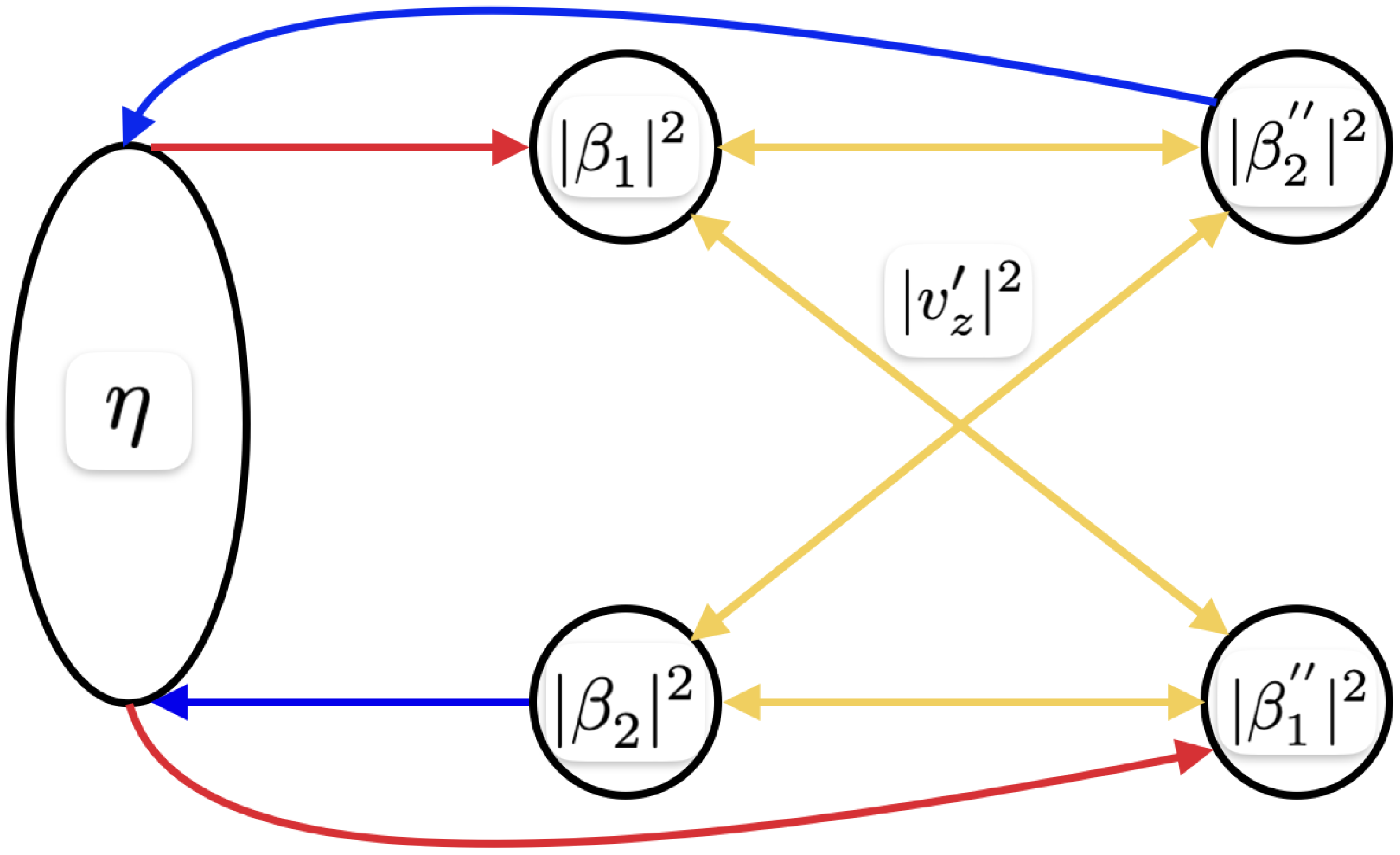
 3−k
3−k β1
β1 β1′′
β1′′ β2
β2 β2′′
β2′′ vz′
vz′ β
β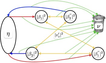
 3−k
3−k β1
β1 β1′′
β1′′ β2
β2 β2′′
β2′′ vz′
vz′ β
β ν
ν ν
ν
 Open access

