


1 Introduction
Dilute plasma beams propagating though ionized background media are ubiquitous in astrophysical plasmas, which themselves span many scales and parameters, e.g. beam-to-background density ratio and beam velocity. Thus, understanding the stability of beam–plasma systems is essential to modelling their evolution and understanding many astrophysical phenomena. Examples include active galactic nuclei (AGNs) driven beam–plasma instabilities in the intergalactic medium (Broderick, Chang & Pfrommer Reference Broderick, Chang and Pfrommer2012), gamma-ray bursts (Ramirez-Ruiz, Nishikawa & Hededal Reference Ramirez-Ruiz, Nishikawa and Hededal2007; Ardaneh et al. Reference Ardaneh, Cai, Nishikawa and Lembége2015), accretion disks around black holes (Riquelme, Quataert & Verscharen Reference Riquelme, Quataert and Verscharen2016), the solar wind (Ginzburg & Zhelezniakov Reference Ginzburg and Zhelezniakov1958), pulsar winds (Weiler & Panagia Reference Weiler and Panagia1978) and relativistic jets from AGNs (Ardaneh, Cai & Nishikawa Reference Ardaneh, Cai and Nishikawa2016; Nishikawa et al. Reference Nishikawa, Frederiksen, Nordlund, Mizuno, Hardee, Niemiec, Gómez, Pe’er, Duţan and Meli2016). To study the stability of such systems, most analytical work has focused on the problem with a uniform background plasma number density. These include studies using both hydrodynamical and more comprehensive kinetic descriptions of beam–plasma systems, see, e.g. Bret, Gremillet & Dieckmann (Reference Bret, Gremillet and Dieckmann2010).
However, it is clear that in some astronomical contexts background inhomogeneity is a critical element. For example, inhomogeneity is necessary to explain the apparent suppression of the non-relativistic plasma beams that are driven during type-III radio bursts (Lin et al. Reference Lin, Potter, Gurnett and Scarf1981). Estimates based on growth rates in the case of uniform background plasmas imply fully thermalized beam particles at 1 AU. In stark contrast, observations show that the beams persist and do not show the expected plateau in their momentum distribution (Lin et al. Reference Lin, Potter, Gurnett and Scarf1981). To explain this, hydrodynamical models of long-wavelength ( $\unicode[STIX]{x1D706}\gg \unicode[STIX]{x1D706}_{D}$, where $\unicode[STIX]{x1D706}_{D}$ is the Debye length) and slowly varying Langmuir waves envelope, i.e. based on the high frequency limit of Zakharov equations (Zakharov Reference Zakharov1972), are developed. These models assume the pre-existence of Langmuir waves, i.e. assume that these are the unstable modes of the system due to the beam propagation; and investigate the evolution of such wave packets in an inhomogeneous medium (Ergun et al. Reference Ergun2008; Krafft, Volokitin & Krasnoselskikh Reference Krafft, Volokitin and Krasnoselskikh2013). These models provide a possible explanation of the observed wave clumping and apparent suppression of the beam instability in type-III radio bursts.
On the other hand, one-dimensional models based on kinetic equations have been developed (Breǐzman & Ruytov Reference Breǐzman and Ruytov1969; Breǐzman & Ryutov Reference Breǐzman and Ryutov1971; Breǐzman, Ryutov & Chebotaev Reference Breǐzman, Ryutov and Chebotaev1972; Nishikawa & Ryutov Reference Nishikawa and Ryutov1976). These models assume the validity of the uniform beam–plasma picture and study how a non-uniform background number density changes the evolution and resonances of the driven Langmuir waves, using the geometric-optic approximation. While these models succeed in explaining observations of type-III radio bursts, i.e. non-relativistic beam–plasma instabilities, they were used by Miniati & Elyiv (Reference Miniati and Elyiv2013) to imply an erroneous suppression of the instabilities in the relativistic regime as shown by Shalaby et al. (Reference Shalaby, Broderick, Chang, Pfrommer, Lamberts and Puchwein2018). Their particle-in-cell (PIC) simulations show a clear growth of the instabilities, very similar to the uniform case.
Here, we revisit both analytically and numerically the growth of longitudinal beam plasma modes using the Vlasov–Poisson system. We assume a quadratic inhomogeneous structure in the background number density and derive the fully relativistic kinetic dispersion relation for this case. We focus on the growth rate of the instability for dilute and cold beams from an initial perturbation, and derive the structure of the unstable modes for such system, i.e. we do not assume pre-existing Langmuir waves. Various predictions, e.g. the rates of wave growth and the shape of the unstable modes, are shown to have an excellent agreement with PIC simulations.
This paper is organized as follows. In § 2, we present the dispersion relation obtained from the linearization of the Vlasov–Poisson equations in the presence of a quadratic background density inhomogeneity. Section 3 drives the normal modes of such inhomogeneous systems in the absence of beam particles. In § 4, we study the effect of weak beams, i.e. the instabilities in the presence of dilute and/or relativistic cold beams, on these normal modes by using analogies with first-order perturbation theory. In § 5, we present a list of predictions from our computation and compare those to PIC simulations using the SHARP code (Shalaby et al. Reference Shalaby, Broderick, Chang, Pfrommer, Lamberts and Puchwein2017b). We discuss the implications of this theory in inhomogeneous intergalactic and solar wind media in § 6, and summarize and conclude in § 7.
2 Formalism
It is often the case that the dynamical time scales for large-scale structures substantially exceeds the relevant plasma time scales for beam–plasma instabilities. This large separation in temporal scales admits a natural simplification of the problem: here, we focus on a beam–plasma system where electron–positron beams are propagating through a denser background of electrons and fixed neutralizing protons. Two illustrative astrophysical applications, the intergalactic medium and solar wind, are presented in § 6, where our assumption of a fixed-background approximation is demonstrated to be an excellent approximation. Nevertheless, we expect this to have broad applicability to beam–plasma situations more generally.
We denote the phase space distribution functions of beam electrons/positrons by  $f^{\pm }$ and for background electrons by $g$. For such a case, the linearized (first-order) Vlasov–Maxwell equations describe the evolution of longitudinal modes, i.e. parallel to the beam direction; for detailed derivation, see, e.g. § 4.2 of Shalaby (Reference Shalaby2017). The resulting equations can be re-written as an eigenvalue problem as follows:
 $$\begin{eqnarray}\left[k+{\displaystyle \frac{e^{2}}{m_{e}\unicode[STIX]{x1D716}_{0}}}\int \text{d}u\frac{\unicode[STIX]{x2202}_{u}(f_{0}^{+}+f_{0}^{-})}{\unicode[STIX]{x1D714}-kv}\right]E_{1}(k,\unicode[STIX]{x1D714})+{\displaystyle \frac{e^{2}}{m_{e}\unicode[STIX]{x1D716}_{0}}}\iint \text{d}k^{\prime }\,\text{d}u\frac{\unicode[STIX]{x2202}_{u}g_{0}(k^{\prime },u)}{\unicode[STIX]{x1D714}-kv}E_{1}(k-k^{\prime },\unicode[STIX]{x1D714})=0.\end{eqnarray}$$
 Here,  $e$ and $m_{e}$ are the elementary charge and mass of electrons respectively, $v$ is the velocity in phase space, $u=\unicode[STIX]{x1D6FE}v$ is the spatial component of the four velocity with Lorentz factor, $\unicode[STIX]{x1D6FE}=1/\sqrt{1-v^{2}/c^{2}}$, $c$ is the speed of light, $f_{0}^{\pm }$ are the equilibrium phase space distribution function of pair-beam plasma particles, $g_{0}$ is the equilibrium phase space distribution function of background electron plasma and $E_{1}$ is the first-order perturbation in the electric field. The convolution in (2.1) complicates finding solutions of this equation. However, this can be greatly simplified when the inhomogeneity has a quadratic structure. Therefore, in the following we consider an inhomogeneity such that the number density of the background electrons is
 $$\begin{eqnarray}\displaystyle n_{g}(x)=n_{0}(1+\unicode[STIX]{x1D716}x^{2}). & & \displaystyle\end{eqnarray}$$
 Assuming that  $g_{0}(x,u)=n_{g}(x)g_{0}(u)$, as, e.g. in an isothermal plasma, we can write
 $$\begin{eqnarray}\displaystyle g_{0}(k^{\prime },u)=n_{0}[\unicode[STIX]{x1D6FF}(k^{\prime })-\unicode[STIX]{x1D716}\unicode[STIX]{x1D6FF}^{\prime \prime }(k^{\prime })]g_{0}(u), & & \displaystyle\end{eqnarray}$$
 where  $\unicode[STIX]{x1D716}$ has dimensions of inverse length squared, and we take $\unicode[STIX]{x1D716}\geqslant 0$, i.e. the inhomogeneity in the number density forms a quadratic bowl with a minimum at $x=0$. In such a case, equation (2.1) can be written as
 $$\begin{eqnarray}\left[k+{\displaystyle \frac{e^{2}}{m_{e}\unicode[STIX]{x1D716}_{0}}}\int \frac{\text{d}u}{\unicode[STIX]{x1D714}-kv}\unicode[STIX]{x2202}_{u}(f_{0}^{+}+f_{0}^{-})\right]E_{1}(k,\unicode[STIX]{x1D714})+\left[\unicode[STIX]{x1D714}_{0}^{2}\int \text{d}u\frac{\unicode[STIX]{x2202}_{u}g_{0}(u)}{\unicode[STIX]{x1D714}-kv}\right](1-\unicode[STIX]{x1D716}\unicode[STIX]{x2202}_{k}^{2})E_{1}(k,\unicode[STIX]{x1D714})=0,\end{eqnarray}$$
 where  $\unicode[STIX]{x1D714}_{0}^{2}=e^{2}n_{0}/(m_{e}\unicode[STIX]{x1D716}_{0})$ is the plasma frequency of the background electrons at $x=0$.
3 Solution without beam
In this case,  $f_{0}^{\pm }=0$, and (2.4) becomes
 $$\begin{eqnarray}\left[k+\unicode[STIX]{x1D714}_{0}^{2}\int \text{d}u\frac{\unicode[STIX]{x2202}_{u}g_{0}(u)}{\unicode[STIX]{x1D714}-kv}\right]E_{1}(k,\unicode[STIX]{x1D714})-\unicode[STIX]{x1D716}\left[\unicode[STIX]{x1D714}_{0}^{2}\int \text{d}u\frac{\unicode[STIX]{x2202}_{u}g_{0}(u)}{\unicode[STIX]{x1D714}-kv}\right]\unicode[STIX]{x2202}_{k}^{2}E_{1}(k,\unicode[STIX]{x1D714})=0.\end{eqnarray}$$
Because the equation is written in the frame of the background electrons, in which they only have thermal motions, the integral in (3.1) can be solved in the non-relativistic limit (Boyd & Sanderson Reference Boyd and Sanderson2003; Chang et al. Reference Chang, Broderick, Pfrommer, Puchwein, Lamberts, Shalaby and Vasil2016),
 $$\begin{eqnarray}\displaystyle \int \text{d}u\frac{\unicode[STIX]{x2202}_{u}g_{0}(u)}{\unicode[STIX]{x1D714}-kv}\sim -\frac{k}{\unicode[STIX]{x1D714}^{2}}\left(1+3\frac{k^{2}\unicode[STIX]{x1D70E}^{2}}{\unicode[STIX]{x1D714}_{0}^{2}}\right), & & \displaystyle\end{eqnarray}$$
 where  $\unicode[STIX]{x1D70E}$ is the thermal width of the background electrons’ momentum distribution, $g_{0}(u)$, which we assume here to be non-relativistic, i.e. $\unicode[STIX]{x1D70E}\ll c$. In deriving (3.2), we consider only long wavelengths compared to the local Debye length $\unicode[STIX]{x1D70E}/\unicode[STIX]{x1D714}_{g}(x)$, where the local plasma frequency is $\unicode[STIX]{x1D714}_{g}(x)=\sqrt{e^{2}n_{g}(x)/\unicode[STIX]{x1D716}_{0}m_{e}}$. However, since the longest Debye length is at the minimum of the density, we define it to be $\unicode[STIX]{x1D706}_{D}=\unicode[STIX]{x1D70E}/\unicode[STIX]{x1D714}_{0}$, and always consider a wavelength much longer than the longest local Debye length $\unicode[STIX]{x1D706}_{D}=\unicode[STIX]{x1D70E}/\unicode[STIX]{x1D714}_{0}$, i.e. $k^{2}\unicode[STIX]{x1D70E}^{2}/\unicode[STIX]{x1D714}_{0}^{2}\ll 1$. Therefore,
 $$\begin{eqnarray}\left(\frac{\unicode[STIX]{x1D714}^{2}}{\unicode[STIX]{x1D714}_{0}^{2}}-1-3\frac{k^{2}\unicode[STIX]{x1D70E}^{2}}{\unicode[STIX]{x1D714}_{0}^{2}}\right)E_{1}+\unicode[STIX]{x1D716}\left(1+3\frac{k^{2}\unicode[STIX]{x1D70E}^{2}}{\unicode[STIX]{x1D714}_{0}^{2}}\right)\unicode[STIX]{x2202}_{k}^{2}E_{1}=0.\end{eqnarray}$$
 If we assume that  $\unicode[STIX]{x1D716}/k_{m}^{2}\leqslant 1$, where $k_{m}$ is the wavenumber of the most important wave mode in the system, i.e. $k_{m}c/\unicode[STIX]{x1D714}_{0}\sim 1$ is the expected fastest unstable mode in the presence of weak pair beams, this ensures that $\unicode[STIX]{x1D716}\unicode[STIX]{x2202}_{k}^{2}E_{1}\leqslant E_{1}$. That is, if the inhomogeneity scale is larger than the plasma skin depth ( $c/\unicode[STIX]{x1D714}_{0}$), we may ignore $k^{2}\unicode[STIX]{x1D70E}^{2}/\unicode[STIX]{x1D714}_{0}^{2}$ in the second term, and write
 $$\begin{eqnarray}-\unicode[STIX]{x2202}_{k}^{2}E_{1}+\frac{3\unicode[STIX]{x1D70E}^{2}}{\unicode[STIX]{x1D716}\unicode[STIX]{x1D714}_{0}^{2}}k^{2}E_{1}=\frac{1}{\unicode[STIX]{x1D716}}\left[\frac{\unicode[STIX]{x1D714}^{2}}{\unicode[STIX]{x1D714}_{0}^{2}}-1\right]E_{1}.\end{eqnarray}$$
 Equation (3.4) has the same structure as the equation for a quantum harmonic oscillator (see, e.g. Shankar Reference Shankar2012; Griffiths Reference Griffiths2016). If we demand that the solution is finite as  $|k|\rightarrow \infty$, we discard the solution of the form $E_{1}(k,\unicode[STIX]{x1D714})\propto \text{e}^{+k^{2}/2a^{2}}$. Thus, the solution is given by
 $$\begin{eqnarray}\displaystyle E_{1}(k,\unicode[STIX]{x1D714})=A_{n}H_{n}(k/a)\text{e}^{-k^{2}/2a^{2}}, & & \displaystyle\end{eqnarray}$$
 where,  $A_{n}$ is a normalization constant, $a^{4}=\unicode[STIX]{x1D716}\unicode[STIX]{x1D714}_{0}^{2}/(3\unicode[STIX]{x1D70E}^{2})=\unicode[STIX]{x1D716}k_{D}^{2}/(3(2\unicode[STIX]{x03C0})^{2})=\unicode[STIX]{x1D716}/3\unicode[STIX]{x1D706}_{D}^{2}$, $k_{D}$ is the wavenumber associated with the Debye length, $\unicode[STIX]{x1D706}_{D}\equiv \unicode[STIX]{x1D70E}/\unicode[STIX]{x1D714}_{0}$, ( $a$ has the dimension of an inverse length) and
 $$\begin{eqnarray}\displaystyle \frac{1}{\unicode[STIX]{x1D716}}\left[\frac{\unicode[STIX]{x1D714}^{2}}{\unicode[STIX]{x1D714}_{0}^{2}}-1\right]=a^{-2}(2n+1),\quad n\in Z^{+}. & & \displaystyle\end{eqnarray}$$
 The bases used in (3.5) are written in terms of wave modes  $k$. However, since the Fourier transform
 $$\begin{eqnarray}{\mathcal{F}}(H_{n}(k)\text{e}^{-k^{2}/2})=(-\text{i})^{n}H_{n}(x)\text{e}^{-x^{2}/2},\end{eqnarray}$$
 the structure of the normal modes, in real space and Fourier space, are similar, see figure 1. Therefore, the solution for each  $n$ is given, in real space, by
 $$\begin{eqnarray}\displaystyle E_{1}(x,\unicode[STIX]{x1D714})=(-\text{i})^{n}A_{n}H_{n}(xa)\text{e}^{-a^{2}x^{2}/2}. & & \displaystyle\end{eqnarray}$$
Comparison of the value of  $H_{n}^{2}(y)\text{e}^{-y^{2}}$ and its approximate form used in (4.10) for $n=30$ (a) and $n=50$ (b). As $n$ increases the number of oscillations near $y=0$ also increases.

Note, demanding that the solution remains finite for  $|k|\rightarrow \infty$, not only excludes the exponentially divergent part of the solution, but also quantizes the remaining part. That is, for only non-negative integer values of $n$ the solution in (3.5) is non-divergent. Thus, the condition in (3.6) represents our dispersion relation. Similar structure of eigenstates was previously found for a quadratic inhomogeneity by Ergun et al. (Reference Ergun2008).
Computing the limit of uniform background plasma from the above formulation is more complicated than just taking the limit  $\unicode[STIX]{x1D716}\rightarrow 0$; equation (3.3) tells us that, in such a limit, the dispersion relation is $\unicode[STIX]{x1D714}^{2}/\unicode[STIX]{x1D714}_{0}^{2}-1=3k^{2}\unicode[STIX]{x1D706}_{D}^{2}$. Since, the dispersion relation in (3.6), can be re-written as
 $$\begin{eqnarray}\displaystyle \left[\frac{\unicode[STIX]{x1D714}^{2}}{\unicode[STIX]{x1D714}_{0}^{2}}-1\right]=\frac{\unicode[STIX]{x1D716}}{a^{2}}(2n+1)=\sqrt{3\unicode[STIX]{x1D716}\unicode[STIX]{x1D706}_{D}^{2}}(2n+1), & & \displaystyle\end{eqnarray}$$
the limit of uniform background plasma can be obtained via
 $$\begin{eqnarray}\unicode[STIX]{x1D716}\rightarrow 0,\quad n\rightarrow \infty \quad \text{such that}~\sqrt{3\unicode[STIX]{x1D716}\unicode[STIX]{x1D706}_{D}^{2}}(2n+1)\rightarrow 3k^{2}\unicode[STIX]{x1D706}_{D}^{2}.\end{eqnarray}$$
By taking the limit in such a way, the solution in (3.8) is reduced to
 $$\begin{eqnarray}E_{1}(x,\unicode[STIX]{x1D714})\propto \cos (kx-n\unicode[STIX]{x03C0}/2),\end{eqnarray}$$
 where we used  $xa\sqrt{2n+1}\rightarrow xa^{2}\sqrt{3k^{2}\unicode[STIX]{x1D706}_{D}^{2}/\unicode[STIX]{x1D716}}=kx$. This is indeed the expected solution in the uniform background case, i.e. the normal modes are Fourier modes rather than Hermite modes. Here, we have used the large- $n$ limit expansion of the Hermite polynomials, and we give an explicit expression in such a limit in (4.9).
4 Adding a weak beam
We now supplement the inhomogeneous background with a weak plasma beam. Here, we assume a cold and uniform pair beam, i.e.
 $$\begin{eqnarray}\displaystyle f_{0}^{\pm }=n_{b}\unicode[STIX]{x1D6FF}(u-u_{b}), & & \displaystyle\end{eqnarray}$$
 where  $n_{b}$ is the uniform number density of the equally dense pair beam, which is defined in the background plasma frame of reference.
Thus, equation (2.4) can be written as
 $$\begin{eqnarray}\left[k-{\displaystyle \frac{e^{2}n_{b}}{m_{e}\unicode[STIX]{x1D716}_{0}}}\frac{2k}{\unicode[STIX]{x1D6FE}_{b}^{3}(\unicode[STIX]{x1D714}-kv_{b})^{2}}\right]E_{1}(k,\unicode[STIX]{x1D714})+\left[\unicode[STIX]{x1D714}_{0}^{2}\int \text{d}u\frac{\unicode[STIX]{x2202}_{u}g_{0}(u)}{\unicode[STIX]{x1D714}-kv}\right](1-\unicode[STIX]{x1D716}\unicode[STIX]{x2202}_{k}^{2})E_{1}(k,\unicode[STIX]{x1D714})=0.\end{eqnarray}$$
 Here,  $\unicode[STIX]{x1D6FE}_{b}$ and $v_{b}$ are the Lorentz factor and the velocity of the pair beam, respectively. We define $\unicode[STIX]{x1D702}=2\unicode[STIX]{x1D6FC}/\unicode[STIX]{x1D6FE}_{b}^{3}$ where $\unicode[STIX]{x1D6FC}=n_{b}/n_{0}$ is the beam-background density ratio at $x=0$. Thus, using (3.2)
 $$\begin{eqnarray}\left[1-\frac{\unicode[STIX]{x1D702}\unicode[STIX]{x1D714}_{0}^{2}}{(\unicode[STIX]{x1D714}-kv_{b})^{2}}\right]E_{1}(k,\unicode[STIX]{x1D714})-\left[\frac{\unicode[STIX]{x1D714}_{0}^{2}}{\unicode[STIX]{x1D714}^{2}}\left(1+3\frac{k^{2}\unicode[STIX]{x1D70E}^{2}}{\unicode[STIX]{x1D714}_{0}^{2}}\right)\right](1-\unicode[STIX]{x1D716}\unicode[STIX]{x2202}_{k}^{2})E_{1}(k,\unicode[STIX]{x1D714})=0.\end{eqnarray}$$
This can be rearranged into
 $$\begin{eqnarray}-\unicode[STIX]{x1D716}\left(1+3\frac{k^{2}\unicode[STIX]{x1D70E}^{2}}{\unicode[STIX]{x1D714}_{0}^{2}}\right)\unicode[STIX]{x2202}_{k}^{2}E_{1}+\left[3\frac{k^{2}\unicode[STIX]{x1D70E}^{2}}{\unicode[STIX]{x1D714}^{2}}+\frac{\unicode[STIX]{x1D702}\unicode[STIX]{x1D714}^{2}}{(\unicode[STIX]{x1D714}-kv_{b})^{2}}\right]E_{1}=\left(\frac{\unicode[STIX]{x1D714}^{2}}{\unicode[STIX]{x1D714}_{0}^{2}}-1\right)E_{1}.\end{eqnarray}$$
 Again, since  $\unicode[STIX]{x1D70E}^{2}k^{2}/\unicode[STIX]{x1D714}_{0}^{2}\ll 1$ and $\unicode[STIX]{x1D716}\unicode[STIX]{x1D706}_{D}^{2}\ll 1$, the thermal correction term in the first parenthesis can be ignored, and we can recast this equation into an equation for a perturbed quantum harmonic oscillator
 $$\begin{eqnarray}-\unicode[STIX]{x2202}_{k}^{2}E_{1}+\left[\frac{3\unicode[STIX]{x1D70E}^{2}}{\unicode[STIX]{x1D716}\unicode[STIX]{x1D714}_{0}^{2}}k^{2}+\frac{\unicode[STIX]{x1D702}\unicode[STIX]{x1D714}^{2}}{\unicode[STIX]{x1D716}(\unicode[STIX]{x1D714}-kv_{b})^{2}}\right]E_{1}=\frac{1}{\unicode[STIX]{x1D716}}\left(\frac{\unicode[STIX]{x1D714}^{2}}{\unicode[STIX]{x1D714}_{0}^{2}}-1\right)E_{1}.\end{eqnarray}$$
 The small perturbation to the potential by the beam term, i.e.  $\unicode[STIX]{x1D702}=2\unicode[STIX]{x1D6FC}/\unicode[STIX]{x1D6FE}_{b}^{3}\ll 1$, means the beam is relativistic and/or dilute. To compute the change in the dispersion relation, we can use the first-order perturbation theory. That is, the eigenvalue condition in (3.6) becomes
 $$\begin{eqnarray}\displaystyle \frac{1}{\unicode[STIX]{x1D716}}\left[\frac{\unicode[STIX]{x1D714}^{2}}{\unicode[STIX]{x1D714}_{0}^{2}}-1\right]=a^{-2}(1+2n)+\unicode[STIX]{x0394}E_{n}, & & \displaystyle\end{eqnarray}$$
where,
 $$\begin{eqnarray}\displaystyle \unicode[STIX]{x0394}E_{n}=\frac{\displaystyle \int \text{d}k{\displaystyle \frac{\unicode[STIX]{x1D702}\unicode[STIX]{x1D714}^{2}}{\unicode[STIX]{x1D716}(\unicode[STIX]{x1D714}-kv_{b})^{2}}}H_{n}^{2}(k/a)\text{e}^{-k^{2}/a^{2}}}{\displaystyle \int \text{d}kH_{n}^{2}(k/a)\text{e}^{-k^{2}/a^{2}}}=\frac{\unicode[STIX]{x1D702}\unicode[STIX]{x1D714}^{2}/\unicode[STIX]{x1D716}}{\displaystyle \int \text{d}yH_{n}^{2}(y)\text{e}^{-y^{2}}}\int \text{d}y\frac{H_{n}^{2}(y)\text{e}^{-y^{2}}}{(\unicode[STIX]{x1D714}-yav_{b})^{2}}, & & \displaystyle\end{eqnarray}$$
 where  $y=k/a$. It is important to note that, in order to find the modified dispersion relation, we use the first-order perturbation theory and explicitly integrate over the Fourier modes labelled by $k$. Thus the dispersion relation becomes independent of $k$. Instead, it depends on $n$, the label for the eigenmodes (the normal modes) of the system in which the electric field perturbation evolves according to (4.5).
Therefore, the full dispersion in the presence of a weak beam ( $\unicode[STIX]{x1D702}\ll 1$) is given by
 $$\begin{eqnarray}\displaystyle \left[\frac{\unicode[STIX]{x1D714}^{2}}{\unicode[STIX]{x1D714}_{0}^{2}}-1\right]=\frac{\unicode[STIX]{x1D716}}{a^{2}}(1+2n)+\unicode[STIX]{x1D702}\frac{b^{2}}{\sqrt{\unicode[STIX]{x03C0}}2^{n}n!}\int \text{d}y\frac{H_{n}^{2}(y)\text{e}^{-y^{2}}}{(y-b)^{2}}, & & \displaystyle\end{eqnarray}$$
 where,  $b=\unicode[STIX]{x1D714}/av_{b}$ and we used $\int \text{d}yH_{n}^{2}(y)\text{e}^{-y^{2}}=\sqrt{\unicode[STIX]{x03C0}}2^{n}n!$.
In the following we are interested only in the growth rates, i.e. the solution of (4.8) with  $\text{Im}[\unicode[STIX]{x1D714}]>0$. Therefore, extending the Landau contours of the integral of (4.8) to the full complex $\unicode[STIX]{x1D714}$-plane is not needed (Ferch & Sudan Reference Ferch and Sudan1975).
4.1 Large- $n$ regime

Here, we approximate the integral in the large- $n$ limit, and also check the regime of validity of such an approximation in appendix B. We use (Abramowitz & Stegun Reference Abramowitz and Stegun1964)
 $$\begin{eqnarray}\displaystyle H_{n}^{2}(y)\text{e}^{-y^{2}}\approx B_{n}\frac{\displaystyle \cos ^{2}\left(y\sqrt{2n+1-{\displaystyle \frac{y^{2}}{3}}}-{\displaystyle \frac{n\unicode[STIX]{x03C0}}{2}}\right)}{\sqrt{1-{\displaystyle \frac{y^{2}}{2n+1}}}}\unicode[STIX]{x1D6E9}\left(1-\frac{y^{2}}{2n+1}\right), & & \displaystyle\end{eqnarray}$$
 where,  $B_{n}=2(2n/e)^{n}$ is a normalization constant and $\unicode[STIX]{x1D6E9}(x)$ is the Heaviside step function. To find a closed form of the dispersion relation in the large- $n$ limit, we need to evaluate the integral in (4.8); we average over the oscillatory part of this approximation first, then evaluate the integrals, i.e.
 $$\begin{eqnarray}\displaystyle \unicode[STIX]{x1D716}\unicode[STIX]{x0394}E_{n}=\frac{\displaystyle \unicode[STIX]{x1D702}b^{2}\int _{-\sqrt{2n+1}}^{\sqrt{2n+1}}\text{d}y\left[1-\frac{y^{2}}{2n+1}\right]^{-1/2}/(b-y)^{2}}{\displaystyle \int _{-\sqrt{2n+1}}^{\sqrt{2n+1}}\text{d}y\left[1-\frac{y^{2}}{2n+1}\right]^{-1/2}}=\frac{\unicode[STIX]{x1D702}b^{3}}{[b^{2}-(2n+1)]^{3/2}}. & & \displaystyle\end{eqnarray}$$
Therefore, the dispersion relation is given by
 $$\begin{eqnarray}\displaystyle \frac{\unicode[STIX]{x1D714}^{2}}{\unicode[STIX]{x1D714}_{0}^{2}}-1=\frac{\unicode[STIX]{x1D716}(2n+1)}{a^{2}}+\frac{\unicode[STIX]{x1D702}b^{3}}{[b^{2}-(2n+1)]^{3/2}}. & & \displaystyle\end{eqnarray}$$
 By defining  $\tilde{\unicode[STIX]{x1D714}}=\unicode[STIX]{x1D714}/\unicode[STIX]{x1D714}_{0}$, $b_{0}=\unicode[STIX]{x1D714}_{0}/av_{b}$ such that $b=\tilde{\unicode[STIX]{x1D714}}b_{0}$, it is also convenient to define $r=(2n+1)/b_{0}^{2}$. Therefore,
 $$\begin{eqnarray}\displaystyle \tilde{\unicode[STIX]{x1D714}}^{2}-1=3\frac{\unicode[STIX]{x1D70E}^{2}}{v_{b}^{2}}r+\frac{\unicode[STIX]{x1D702}\tilde{\unicode[STIX]{x1D714}}^{3}}{(\tilde{\unicode[STIX]{x1D714}}^{2}-r)^{3/2}}, & & \displaystyle\end{eqnarray}$$
 where we used  $a^{2}=\unicode[STIX]{x1D716}\unicode[STIX]{x1D714}_{0}^{2}/3\unicode[STIX]{x1D70E}^{2}a^{2}$ or, equivalently $\unicode[STIX]{x1D716}/a^{2}=3(\unicode[STIX]{x1D70E}^{2}/v_{b}^{2})/b_{0}^{2}$.
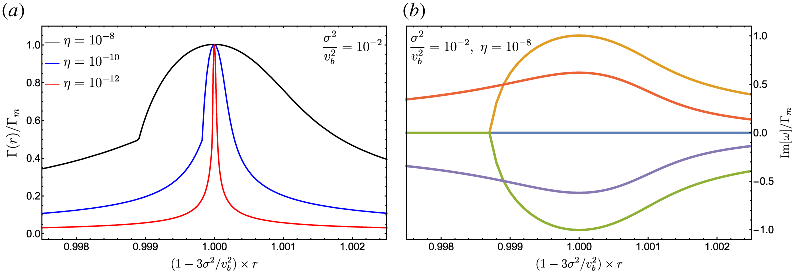
Numerical solutions of the dispersion relation in the large- $n$ limit. (a) We show the fastest growth rate obtained by solving (4.12) and numerically normalize it to the fastest growth rate, $\unicode[STIX]{x1D6E4}_{m}$, given by (4.16). This is shown for $\unicode[STIX]{x1D70E}^{2}/v_{b}^{2}=10^{-2}$, and various values of $\unicode[STIX]{x1D702}$ ( $\unicode[STIX]{x1D702}=10^{-8}$, $10^{-10}$ and $10^{-12}$). (b) We show all solutions of $\text{Im}[\unicode[STIX]{x1D714}]$ for the case of $\unicode[STIX]{x1D70E}^{2}/v_{b}^{2}=10^{-2}$ and $\unicode[STIX]{x1D702}=10^{-8}$. Panel (b) shows that the kink features in the fastest growth rate curves of the panel (a) are a result of switching between different unstable branches. Here, $r=(2n+1)/b_{0}=(2n+1)v_{b}a/\unicode[STIX]{x1D714}_{0}$, and $a^{4}=\unicode[STIX]{x1D716}\unicode[STIX]{x1D714}_{0}^{2}/3\unicode[STIX]{x1D70E}^{2}$.
4.1.1 Fastest growing modes
When  $\unicode[STIX]{x1D702}=0$, i.e. no beam case, the solution of the dispersion relation is $\tilde{\unicode[STIX]{x1D714}}^{2}=\tilde{\unicode[STIX]{x1D714}}_{0}^{2}=1+3\unicode[STIX]{x1D70E}^{2}r/v_{b}^{2}$. Since the beam term is such that $\unicode[STIX]{x1D702}\ll 1$, the solution of the full dispersion relation should be such that $\tilde{\unicode[STIX]{x1D714}}=\tilde{\unicode[STIX]{x1D714}}_{0}+\unicode[STIX]{x1D6FF}\tilde{\unicode[STIX]{x1D714}}$, where $|\unicode[STIX]{x1D6FF}\tilde{\unicode[STIX]{x1D714}}|\ll \tilde{\unicode[STIX]{x1D714}}_{0}$. Therefore, to lowest order in $\unicode[STIX]{x1D6FF}\tilde{\unicode[STIX]{x1D714}}$, the dispersion relation can be recast as
 $$\begin{eqnarray}\displaystyle \tilde{\unicode[STIX]{x1D714}}_{0}^{2}-1-3\frac{\unicode[STIX]{x1D70E}^{2}}{v_{b}^{2}}r+2\unicode[STIX]{x1D6FF}\tilde{\unicode[STIX]{x1D714}}=2\unicode[STIX]{x1D6FF}\tilde{\unicode[STIX]{x1D714}}=\frac{\unicode[STIX]{x1D702}\tilde{\unicode[STIX]{x1D714}}^{3}}{(\tilde{\unicode[STIX]{x1D714}}^{2}-r)^{3/2}}\approx \frac{\unicode[STIX]{x1D702}}{(\tilde{\unicode[STIX]{x1D714}}_{0}^{2}+2\unicode[STIX]{x1D6FF}\tilde{\unicode[STIX]{x1D714}}-r)^{3/2}}. & & \displaystyle\end{eqnarray}$$
 It is easy to show that  $\text{Im}\{\unicode[STIX]{x1D6FF}\tilde{\unicode[STIX]{x1D714}}\}$ is maximized when $\tilde{\unicode[STIX]{x1D714}}_{0}^{2}-r=0$. That is, the fastest growing mode occurs at $r=r_{m}$, and is such that
 $$\begin{eqnarray}\displaystyle r_{m}=1+3\unicode[STIX]{x1D70E}^{2}r_{m}/v_{b}^{2}~\Rightarrow ~r_{m}=\frac{1}{1-3{\displaystyle \frac{\unicode[STIX]{x1D70E}^{2}}{v_{b}^{2}}}}\approx 1+3\frac{\unicode[STIX]{x1D70E}^{2}}{v_{b}^{2}}. & & \displaystyle\end{eqnarray}$$
 Figure 2(a) shows an excellent agreement between  $r_{m}$ and the value of $r$ where the growth rate is maximum when the full dispersion relation is solved numerically. Therefore, the fastest growth rate is such that
 $$\begin{eqnarray}\displaystyle 2\unicode[STIX]{x1D6FF}\tilde{\unicode[STIX]{x1D714}}\sim \frac{\unicode[STIX]{x1D702}}{(2\unicode[STIX]{x1D6FF}\tilde{\unicode[STIX]{x1D714}})^{3/2}}~\Rightarrow ~\unicode[STIX]{x1D6FF}\tilde{\unicode[STIX]{x1D714}}\sim \frac{\unicode[STIX]{x1D702}^{2/5}}{2}\left\{1,\cos \frac{2\unicode[STIX]{x03C0}}{5}\pm \text{i}\sin \frac{2\unicode[STIX]{x03C0}}{5},\cos \frac{4\unicode[STIX]{x03C0}}{5}\pm \text{i}\sin \frac{4\unicode[STIX]{x03C0}}{5}\right\},\qquad & & \displaystyle\end{eqnarray}$$
and the maximum growth rate is
 $$\begin{eqnarray}\displaystyle \unicode[STIX]{x1D6E4}_{m}\sim \frac{\unicode[STIX]{x1D702}^{2/5}}{2}\sin \frac{2\unicode[STIX]{x03C0}}{5}\unicode[STIX]{x1D714}_{0}. & & \displaystyle\end{eqnarray}$$
 The computed maximum growth rate in (4.16) is in excellent agreement with the fastest growth rate that is found by numerically solving the full dispersion relation near  $r=r_{m}$ (see figure 2a).
To compute the eigenmode where the fastest growth occurs  $n_{m}$, we use
 $$\begin{eqnarray}r_{m}=\frac{2n_{m}+1}{b_{0}^{2}}=(2n_{m}+1)\frac{v_{b}^{2}a^{2}}{\unicode[STIX]{x1D714}_{0}^{2}}=(2n_{m}+1)(v_{b}/\unicode[STIX]{x1D70E})^{2}\sqrt{\frac{\unicode[STIX]{x1D716}\unicode[STIX]{x1D706}_{D}^{2}}{3}}\approx 1+3\frac{\unicode[STIX]{x1D70E}^{2}}{v_{b}^{2}},\end{eqnarray}$$
 where,  $\unicode[STIX]{x1D706}_{D}=\unicode[STIX]{x1D70E}/\unicode[STIX]{x1D714}_{0}$. The fastest growth occurs at
 $$\begin{eqnarray}\displaystyle 2n_{m}+1=b_{0}^{2}\left(1+3\frac{\unicode[STIX]{x1D70E}^{2}}{v_{b}^{2}}\right)=\frac{\sqrt{3/\unicode[STIX]{x1D716}\unicode[STIX]{x1D706}_{D}^{2}}}{(v_{b}/\unicode[STIX]{x1D70E})^{2}}\left(1+3\frac{\unicode[STIX]{x1D70E}^{2}}{v_{b}^{2}}\right)=\sqrt{\frac{3}{\unicode[STIX]{x1D716}\unicode[STIX]{x1D706}_{D}^{2}}}\left(\frac{\unicode[STIX]{x1D70E}^{2}}{v_{b}^{2}}+3\frac{\unicode[STIX]{x1D70E}^{4}}{v_{b}^{4}}\right).\quad & & \displaystyle\end{eqnarray}$$
 Therefore, the condition to find  $n_{m}$ in the large- $n$ limit, i.e. the growth in the presence of such an inhomogeneity is (using $\unicode[STIX]{x1D70E}\ll v_{b}$)
 $$\begin{eqnarray}\displaystyle 2n_{m}\gg 0~\Rightarrow ~\sqrt{\frac{3}{\unicode[STIX]{x1D716}\unicode[STIX]{x1D706}_{D}^{2}}}\approx \frac{\sqrt{3}L_{\text{inh}}}{\unicode[STIX]{x1D706}_{D}}\gg \frac{v_{b}^{2}}{\unicode[STIX]{x1D70E}^{2}}, & & \displaystyle\end{eqnarray}$$
 where  $L_{\text{inh}}\equiv 1/\sqrt{\unicode[STIX]{x1D716}}$ is the typical length scale over which the density changes substantially. It is worth noting that because, in the large- $n$ limit, $r_{m}\sim O(1)$, the large- $n$ limit is equivalent to the large- $b_{0}^{2}$ limit. The fastest growth rate of the longitudinal modes, when the background density is uniform, is given by (Bret et al. Reference Bret, Gremillet and Dieckmann2010; Broderick et al. Reference Broderick, Chang and Pfrommer2012)
 $$\begin{eqnarray}\displaystyle \unicode[STIX]{x1D6E4}_{\text{uniform}}={\displaystyle \frac{\sqrt{3}}{2}}{\displaystyle \frac{\unicode[STIX]{x1D6FC}^{1/3}}{\unicode[STIX]{x1D6FE}_{b}}}\unicode[STIX]{x1D714}_{g}={\displaystyle \frac{\sqrt{3}}{2^{4/3}}}\unicode[STIX]{x1D702}^{1/3}\unicode[STIX]{x1D714}_{g}, & & \displaystyle\end{eqnarray}$$
 where,  $\unicode[STIX]{x1D714}_{g}=\sqrt{n_{g}e^{2}/m_{e}\unicode[STIX]{x1D716}_{0}}$, is the plasma frequency of the background electrons in the uniform case that we want to compare to. Therefore, using (4.16), the growth rate in the presence of an inhomogeneity is reduced by a small factor that is given by
 $$\begin{eqnarray}\displaystyle \frac{\unicode[STIX]{x1D6E4}_{m}}{\unicode[STIX]{x1D6E4}_{\text{uniform}}}=\frac{\unicode[STIX]{x1D714}_{0}}{\unicode[STIX]{x1D714}_{g}}\frac{2^{1/3}\sin \left({\displaystyle \frac{2\unicode[STIX]{x03C0}}{5}}\right)}{\sqrt{3}}\unicode[STIX]{x1D702}^{1/15}. & & \displaystyle\end{eqnarray}$$
4.1.2 Instability spectral width
From the numerical solution of (4.12) (see figure 2), we find that the full-width half-max, i.e. the width in  $r$ where all the growth is within a factor 0.5 of the fastest growth rate, can be well approximated by
 $$\begin{eqnarray}\displaystyle \unicode[STIX]{x0394}r\sim 2.5\unicode[STIX]{x1D702}^{2/5}~\Rightarrow ~\unicode[STIX]{x0394}n=1.25\unicode[STIX]{x1D702}^{2/5}\frac{\unicode[STIX]{x1D70E}^{2}}{v_{b}^{2}}\sqrt{\frac{3}{\unicode[STIX]{x1D716}\unicode[STIX]{x1D706}_{D}^{2}}}=1.25b_{0}^{2}\unicode[STIX]{x1D702}^{2/5}. & & \displaystyle\end{eqnarray}$$
 That is, the weaker the beam gets (smaller  $\unicode[STIX]{x1D702}$), the slower the fastest growth rate, and the smaller the spectral support around the fastest growing mode, $n_{m}$.
4.2 Low-$n$ regime

A systematic method to analytically compute the dispersion relations is given in appendix A. Explicit equations for the dispersion relation at  $n=0,1,2,3$ are given in table 1, in terms of
 $$\begin{eqnarray}{\mathcal{I}}_{0}(b)=2\unicode[STIX]{x03C0}b\text{e}^{-b^{2}}[\text{Erfi}(b)-\text{i}]-2\sqrt{\unicode[STIX]{x03C0}}.\end{eqnarray}$$
 For parameters relevant for the inhomogeneity in type-III radio burst environments ( $3\unicode[STIX]{x1D70E}^{2}/v_{b}^{2}=10^{-3}$ and $\unicode[STIX]{x1D702}=10^{-5}$), we show the roots near $\unicode[STIX]{x1D714}=\unicode[STIX]{x1D714}_{0}$ of some of these dispersion relations up to $n=19$ in figure 3. The light-blue shaded region in figure 3 indicates the range of values of inhomogeneities, characterized by $b_{0}$, in the context of type-III radio bursts (Reid & Ratcliffe Reference Reid and Ratcliffe2014).
Growth rates found by solving the dispersion relation in (4.8), near  $\text{Im}[\unicode[STIX]{x1D714}]=0$, for various eigenmodes $n$. Note, because roots are found near $\unicode[STIX]{x1D714}=\unicode[STIX]{x1D714}_{0}$, $\text{Im}[\unicode[STIX]{x1D714}]$ is not necessarily the fastest growth rate. $\unicode[STIX]{x1D6E4}_{\text{uniform}}$ is the linear growth rate when the background plasma is uniform (given by (4.20)). These solutions are shown for a beam with $3\unicode[STIX]{x1D70E}^{2}/v_{b}^{2}=10^{-3}$ and $\unicode[STIX]{x1D702}=10^{-5}$ (parameters relevant for the inhomogeneities in type-III radio burst environments). The light-blue shaded region indicates the range of inhomogeneities in these environments, see § 6.2.

Low  $n$ dispersion relations. Here, $\tilde{\unicode[STIX]{x1D714}}=\unicode[STIX]{x1D714}/\unicode[STIX]{x1D714}_{0}$, $b=\unicode[STIX]{x1D714}/av_{b}=\tilde{\unicode[STIX]{x1D714}}b_{0}$, where $b_{0}^{2}=\unicode[STIX]{x1D714}_{0}^{2}/a^{2}v_{b}^{2}=(\unicode[STIX]{x1D70E}^{2}/v_{b}^{2})\sqrt{3/\unicode[STIX]{x1D716}\unicode[STIX]{x1D706}_{D}^{2}}$, ${\mathcal{I}}_{0}(b)$ is given in (4.23) and we used $\unicode[STIX]{x1D716}(2n+1)/a^{2}=(3\unicode[STIX]{x1D70E}^{2}/v_{b}^{2})[(2n+1)/b_{0}^{2}]$.
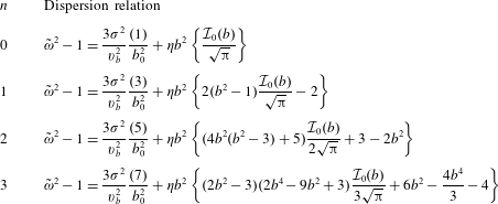
The analytical forms of the dispersion relation found here are polynomials typically of order  ${>}4$, i.e. for $n>1$, these polynomials multiply ${\mathcal{I}}_{0}$ which contain $\text{Erfi}(b)$. Thus, finding all roots of this dispersion relation is tedious. To find the fastest growing modes, one would need to solve for all roots of the dispersion relation, and find the solution with the largest growth rate. This is a complicated process and we leave this for future workFootnote 1.
4.3 Size of unstable region
An important prediction of the computation of this section is that unstable modes are restricted to finite ranges in (position) space. That is, if the most unstable state is the eigenmode with  $n_{m}$, the number of peaks, for modes of the form given by (3.8), is $n_{m}+1$. The mode and its instability are then restricted to the region between the two outermost peaks (see figure 1 which illustrates the shape of this function).
The width of the unstable region, i.e. the distance between the furthest peaks, is  $2x_{c}$ such that (using (3.8))
 $$\begin{eqnarray}\displaystyle a^{2}x_{c}^{2}=2n_{m}+1~\Rightarrow ~x_{c}^{2}=\frac{(2n_{m}+1)\unicode[STIX]{x1D714}_{0}^{2}}{v_{b}^{2}a^{2}}\left(\frac{c}{\unicode[STIX]{x1D714}_{0}}\right)^{2}\left(\frac{v_{b}}{c}\right)^{2}=(2n_{m}+1)b_{0}^{2}(v_{b}/c)^{2}\frac{c^{2}}{\unicode[STIX]{x1D714}_{0}^{2}}.\qquad & & \displaystyle\end{eqnarray}$$
Therefore,
 $$\begin{eqnarray}\displaystyle \frac{x_{c}}{c/\unicode[STIX]{x1D714}_{0}}=b_{0}\frac{v_{b}}{c}\sqrt{2n_{m}+1}. & & \displaystyle\end{eqnarray}$$
To facilitate following the application of our computations, in table 2, we list the most important variables used throughout this work. The table also gives various definitions and indications to the significance for some of these variables.
A list of important variables and definitions used throughout this work.

5 Comparisons with numerical simulations
Here, we compare our analytical computations of § 4 with PIC simulations of the beam–plasma instability using the SHARP code Shalaby et al. (Reference Shalaby, Broderick, Chang, Pfrommer, Lamberts and Puchwein2017b).
5.1 Analytical predictions and limitations
Before presenting our simulations, it is worth noting that all our calculations in this paper assumed that the pair beams are cold. However, in order to avoid the known numerical heating (see e.g. Birdsall & Maron Reference Birdsall and Maron1980), the pair beams are initialized in the simulations with a non-relativistic thermal temperature of  $k_{B}T_{b}=10^{-4}m_{e}c^{2}$ in the beam rest frame. Thus, we only expect an agreement with our analytical computation for beams moving with relativistic speeds. For beams that are moving at non-relativistic speeds, additional thermal effects are expected to alter the growth of the unstable modes.
The motivation for our simulations is to compare the results against various predictions of our calculation in § 4. We list these predictions below:
(i) Fastest growth rate: it is practically difficult to find such a rate in the low-
$n$ limit, thus we use the growth rates computed in the large-$n$ limit for reference, i.e. equation (4.16).(ii) A given fastest growth state
$n_{m}$ has $n_{m}+1$ peaks whose wavelengths increase near cutoff in real space, $\pm x_{c}$.(iii) For a given fastest growth state
$n_{m}$, the size of growth region, $2x_{c}$, is determined by (4.25). This is another prediction from our computation and is independent of whether $n_{m}$ is computed by solving the dispersion relation or found by counting the number of peaks in the simulation.(iv) For non-relativistic beams, the thermal effects from the beam particles are important in the linear regime, and thus, the evolution is expected to be different (e.g. suppressed) in comparison to our computation that assumes cold beams.


5.2 Particle-in-cell simulations
Here, we present 1D1V (one-dimensional in position and one-dimensional in velocity) PIC simulations with a quadratic density inhomogeneity for high and low values of  $b_{0}\equiv \sqrt{(\unicode[STIX]{x1D70E}^{2}/v_{b}^{2})\sqrt{3/\unicode[STIX]{x1D716}\unicode[STIX]{x1D706}_{D}^{2}}}\sim 31.675$, 3.38 and 1.49. For all simulations, the background plasma is composed of stationary thermal electron plasma, and a fixed neutralizing background, i.e. simulations are performed in the background plasma frame of reference. The beam-to-background density ratio $\unicode[STIX]{x1D6FC}=0.002$. Such a low value of $\unicode[STIX]{x1D6FC}$ facilitates a direct comparison between the results of these simulations to our analytical results in § 4. For all cases, the initial normalized background number density (for both electrons and the fixed neutralizing background), on a computational domain of length $L$, is given by
 $$\begin{eqnarray}\frac{n(x)}{n_{g}}=\frac{1+\unicode[STIX]{x1D716}(x-L/2)^{2}}{1+\unicode[STIX]{x1D716}L^{2}/12},\end{eqnarray}$$
 where  $n_{g}$ is the average number density of the simulated plasmas. Periodic boundary condition on particles and fields are used, and the pair beams are initially spatially uniform and have a non-relativistic (rest-frame) temperature of $k_{B}T_{b}=10^{-4}m_{e}c^{2}$. The level of inhomogeneity in these simulations, which sets the size of the simulation domain, $L$, depends on the velocity of the beam, $v_{b}$ and the background electron thermal velocity, $\unicode[STIX]{x1D70E}$. The inhomogeneity parameter $\unicode[STIX]{x1D716}$ in units of the plasma skin depth is given by
 $$\begin{eqnarray}\displaystyle \unicode[STIX]{x1D716}\frac{c^{2}}{\unicode[STIX]{x1D714}_{p}^{2}}=\left(\frac{\unicode[STIX]{x1D714}_{0}}{\unicode[STIX]{x1D714}_{p}}\right)^{2}\frac{3(\unicode[STIX]{x1D70E}/c)^{2}}{b_{0}^{4}(v_{b}/c)^{4}}. & & \displaystyle\end{eqnarray}$$
 In all simulations, we resolve the plasma skin depth by 10 cells, i.e.  $\unicode[STIX]{x0394}x=0.1c/\unicode[STIX]{x1D714}_{p}$, where $\unicode[STIX]{x1D714}_{p}$ is the plasma frequency of all simulated species. The time step is fixed and is such that $c\unicode[STIX]{x0394}t/\unicode[STIX]{x0394}x=0.4$. We use a fifth-order interpolation scheme for both the deposition and back interpolation steps, which greatly improves the energy conservation of the simulations, see Shalaby et al. (Reference Shalaby, Broderick, Chang, Pfrommer, Lamberts and Puchwein2017b) for a more detailed discussion on this issue.
A proper way to study the convergence behaviour of PIC simulations in such cases is derived in Shalaby et al. (Reference Shalaby, Broderick, Chang, Pfrommer, Lamberts and Puchwein2017a,Reference Shalaby, Broderick, Chang, Pfrommer, Lamberts and Puchweinb). Such convergence studies, however, go beyond the scope of this paper. We here use our simulations only to demonstrate the agreement between them and the calculated linear instability in the presence of a quadratic inhomogeneity in the background electron plasma.
5.2.1 High $b_{0}$, with relativistic beam: $\text{Hb0}\text{-}\text{rel}$


For this simulation, we initialize an electron–positron beam with relativistic speed  $v_{b}/c=0.99995$, i.e. $\unicode[STIX]{x1D6FE}_{b}\sim 100$, the initial background temperature is such that $\unicode[STIX]{x1D70E}^{2}/v_{b}^{2}=10^{-2}$. The pair beams are initialized with a fixed number of 20 particles per cell for each species, while the average number of background electrons per cell is $10^{4}$. The level of inhomogeneity is $\unicode[STIX]{x1D716}c^{2}/\unicode[STIX]{x1D714}_{p}^{2}\sim 2.98\times 10^{-8}$, i.e. a very weak inhomogeneity. This corresponds to $b_{0}\sim 31.675$. That is, the growth rate of this simulation is expected to be directly comparable to results found in the large- $n$ limit (see § 4.1).
Therefore, using (4.17), (4.21) and (4.25)
 $$\begin{eqnarray}n_{m}\sim \frac{b_{0}^{2}}{2}\left(1+3\frac{\unicode[STIX]{x1D70E}^{2}}{v_{b}^{2}}\right)\sim 515,\quad \frac{\unicode[STIX]{x1D6E4}_{m}}{\unicode[STIX]{x1D714}_{0}}\sim 2.08\times 10^{-4},\quad \frac{\unicode[STIX]{x1D6E4}_{m}}{\unicode[STIX]{x1D6E4}_{\text{uniform}}}\sim 0.18,\quad 2x_{c}\sim 2047\frac{c}{\unicode[STIX]{x1D714}_{p}}.\end{eqnarray}$$
 Because of this, we choose the box size to be  $L=7500c/\unicode[STIX]{x1D714}_{p}\gg 2x_{c}$.
The ratio of the best-fitting growth rate of the potential energy (i.e.  $\unicode[STIX]{x1D6E4}_{m}t\in [3.6,5]$) in our numerical simulation in comparison to the theoretically expected growth rate is 1.22. This good agreement between the theoretically expected and numerically simulated growth rates is shown in figure 4(a,b) (red curves).
Particle-in-cell simulation results. (a) Growth of the potential energy density per computation particle,  ${\mathcal{E}}$, (normalized to $m_{e}c^{2}$), in various simulations. The time is normalized to the expected growth rate in the large- $n$ limit $\unicode[STIX]{x1D6E4}_{\text{m}}$, i.e. given in (4.16). For Lb0-nonrel, the time is further divided by a factor of 100. (b) The evolution of percentage energy loss by beam particles in various simulations. (c) The absolute value of the charge density on the grid at $\unicode[STIX]{x1D6E4}_{m}t\sim 3.2$, i.e. near the end of the linear regime potential energy growth (a) of the Lb0-rel simulation. Since the unstable modes are travelling along the beam direction ( $+x$-direction), their reflection (see, e.g. figure 4 of Shalaby et al. Reference Shalaby, Broderick, Chang, Pfrommer, Lamberts and Puchwein2018) at higher-density regions, i.e. $|x|>0$, results in an asymmetric structure, as shown in (c).

5.2.2 Low $b_{0}$, with relativistic beam: $\text{Lb0}\text{-}\text{rel}$


In this simulation, we initialize an electron–positron beam that is moving with relativistic speed  $v_{b}/c=0.99995$, i.e. $\unicode[STIX]{x1D6FE}_{b}\sim 100$, and the initial background temperature is such that $\unicode[STIX]{x1D70E}^{2}/v_{b}^{2}=10^{-3}$. The pair beams are initialized with a fixed number of 40 particles per cell for each species, while the average number of background electrons per cell is $2\times 10^{4}$. That is, the level of inhomogeneity is $\unicode[STIX]{x1D716}c^{2}/\unicode[STIX]{x1D714}_{p}^{2}\sim 1.16\times 10^{-5}$, i.e. a strong inhomogeneity. This corresponds to $b_{0}=3.38$.
Solutions such as the ones shown in figure 3 show that the most unstable eigenmode is  $n_{m}=9$, thus the expected number of peaks during the linear evolution in the charge density is 10. the region where such growth is given by (4.25); $x_{c}=20.69c/\unicode[STIX]{x1D714}_{p}$.
Excellent agreement between the predicted number of peaks and the size of the growth region is show in figure 4(c). Moreover, the ratio of the best-fitting growth rate of the potential energy (i.e.  $\unicode[STIX]{x1D6E4}_{m}t\in [3.6,5]$) in our numerical simulation in comparison to the theoretically expected growth rate is 1.2. That is, we see a good agreement between the theoretically expected (large- $n$ limit) and numerically simulated growth rates of the simulation. This is shown in figure 4(a) (blue curves).
5.2.3 Low $b_{0}$, with non-relativistic beam: $\text{Lb0}\text{-}\text{nonrel}$


In this simulation, we initialize an electron–positron beam that is moving at non-relativistic speed  $v_{b}/c=0.1$, and the initial background temperature is such that $\unicode[STIX]{x1D70E}^{2}/v_{b}^{2}=0.099$. The pair beams are initialized with a fixed number of particles per cell of $10^{3}$ per species, while the average number of background electrons per cell is $5\times 10^{5}$. That is, the level of inhomogeneity is $\unicode[STIX]{x1D716}c^{2}/\unicode[STIX]{x1D714}_{p}^{2}\sim 0.084$, i.e. a very strong inhomogeneity. This corresponds to $b_{0}=1.49$.
Naive application of our results above suggests a non-trivial growth rate, which is not seen in the numerical calculation. We attribute this to the violation of the cold-beam approximation in our analytic calculation and suggest that thermal effects of the beam-particle momentum distribution almost completely suppress the growth in such a case (magenta curves in figure 4).
6 Applications
Here, we apply the results of § 4, to astrophysical plasmas within various astrophysical contexts that span many scales while adhering to its limitations found in § 5. This is done with the goal of determining whether the inhomogeneity, with the structure studied here, can suppress the growth of the unstable wave modes.
6.1 Beam–plasma instabilities in the intergalactic medium
The TeV photons emitted by blazars create, via pair production, very energetic pair beams that propagate through the ionized intergalactic medium (IGM) (Broderick et al. Reference Broderick, Chang and Pfrommer2012; Chang, Broderick & Pfrommer Reference Chang, Broderick and Pfrommer2012; Pfrommer, Chang & Broderick Reference Pfrommer, Chang and Broderick2012; Puchwein et al. Reference Puchwein, Pfrommer, Springel, Broderick and Chang2012; Broderick et al. Reference Broderick, Pfrommer, Puchwein and Chang2014). Fermi-LAT observations at GeV energies show that the expected GeV photons that result from the inverse Compton cascade of these pair beams on cosmic microwave photons are missing (Broderick et al. Reference Broderick, Tiede, Shalaby, Pfrommer, Puchwein, Chang and Lamberts2016; Tiede et al. Reference Tiede, Broderick, Shalaby, Pfrommer, Puchwein, Chang and Lamberts2017a,Reference Tiede, Broderick, Shalaby, Pfrommer, Puchwein, Chang and Lambertsb; Ackermann et al. Reference Ackermann, Ajello, Baldini, Ballet, Barbiellini, Bastieri, Bellazzini, Bissaldi, Blandford and Bloom2018; Broderick et al. Reference Broderick, Tiede, Chang, Lamberts, Pfrommer, Puchwein, Shalaby and Werhahn2018). A plausible explanation of such a mystery is that virulent kinetic plasma instabilities in the IGM, induced by the pair beams, reduce the pair-beam energy on time scales much shorter than that of the inverse Compton cascade. The validity of such a scenario strongly depends on the nonlinear saturation of these instabilities (Miniati & Elyiv Reference Miniati and Elyiv2013; Chang et al. Reference Chang, Broderick, Pfrommer, Puchwein, Lamberts and Shalaby2014; Sironi & Giannios Reference Sironi and Giannios2014; Chang et al. Reference Chang, Broderick, Pfrommer, Puchwein, Lamberts, Shalaby and Vasil2016; Kempf, Kilian & Spanier Reference Kempf, Kilian and Spanier2016; Shalaby et al. Reference Shalaby, Broderick, Chang, Pfrommer, Lamberts and Puchwein2017a; Vafin et al. Reference Vafin, Rafighi, Pohl and Niemiec2018, Reference Vafin, Deka, Pohl and Bohdan2019).
It was suggested by Miniati & Elyiv (Reference Miniati and Elyiv2013) that the inhomogeneity in the IGM number density can potentially suppress the growth of such instabilities. However, it was demonstrated with PIC simulations that the condition for suppressing the instabilities computed in Miniati & Elyiv (Reference Miniati and Elyiv2013) is invalid, and cannot suppress even the slowest type of instabilities in such systems, i.e. the longitudinal instability (Shalaby et al. Reference Shalaby, Broderick, Chang, Pfrommer, Lamberts and Puchwein2018).
Our assumption of a fixed background is exceedingly well justified in voids within the IGM. The dynamical time scale over which gravitational instabilities will modify inhomogeneities in low-density regions is greater than  $10^{11}$ years. In comparison, estimates for the typical growth time scales for blazar-driven beam–plasma instabilities range from $10^{3}$ to $10^{5}$ years (Broderick et al. Reference Broderick, Chang and Pfrommer2012). As we will see below, the growth time estimates are not substantially changed in presence of inhomogeneities, and thus over many growth times a fixed background is an excellent approximation.
Below, we use our computed growth rates to demonstrate that the level of inhomogeneity in the IGM (for inhomogeneities of the structure studied in this work) is indeed not sufficient to suppress the longitudinal instability driven by the pair beams in the IGM. The relevant parameters for such a situation are  $v_{b}\sim c$, and the background temperature of electrons of the IGM is such that $\unicode[STIX]{x1D70E}/c\sim \unicode[STIX]{x1D70E}/v_{b}=7.5\times 10^{-3}$. The inhomogeneity scale length is $L_{\text{inh}}\approx 10^{2}{-}10^{3}$ kpc at mean density (Miniati & Elyiv Reference Miniati and Elyiv2013). The Debye length is $\unicode[STIX]{x1D706}_{D}\sim 84~\text{km}$. Thus
 $$\begin{eqnarray}\displaystyle \frac{\sqrt{3}L_{\text{inh}}}{\unicode[STIX]{x1D706}_{D}}\approx 6.4\times (10^{16}-10^{17}),\quad \frac{\unicode[STIX]{x1D70E}^{2}}{v_{b}^{2}}\approx 5.6\times 10^{-5}. & & \displaystyle\end{eqnarray}$$
Thus, the conditions underlying the analysis in § 4 are satisfied. The index of the fastest growing wave mode, using (4.19), is given by
 $$\begin{eqnarray}\displaystyle n_{m}=\sqrt{\frac{3}{4}\frac{L_{\text{inh}}}{\unicode[STIX]{x1D706}_{D}}}\left(\frac{\unicode[STIX]{x1D70E}^{2}}{v_{b}^{2}}+3\frac{\unicode[STIX]{x1D70E}^{4}}{v_{b}^{4}}\right)-\frac{1}{2}\approx (1-3)\times 10^{4}, & & \displaystyle\end{eqnarray}$$
 placing the blazar-driven beam–plasma instabilities well within the large- $n$ regime. For the longitudinal modes we studied here, $\unicode[STIX]{x1D702}=\unicode[STIX]{x1D6FC}/\unicode[STIX]{x1D6FE}_{b}^{2}$, however, for the blazar-driven beam–plasma instabilities, the oblique modes are the fastest unstable linear modes for which $\unicode[STIX]{x1D702}=\unicode[STIX]{x1D6FC}/\unicode[STIX]{x1D6FE}_{b}$ (Bret et al. Reference Bret, Gremillet and Dieckmann2010). The typical parameters for these instabilities are $\unicode[STIX]{x1D6FC}=10^{-16}$ and $\unicode[STIX]{x1D6FE}_{b}=10^{6}$, thus, the expected reduction to the growth rate is roughly $10^{(-16-6)/15}\sim 1/40$. As a result, the inhomogeneity is unlikely to suppress the linear growth of the blazar-driven beam–plasma instability in the IGM in the cold-beam limit.
Application to the ‘cosine’ simulation of Shalaby et al. (Reference Shalaby, Broderick, Chang, Pfrommer, Lamberts and Puchwein2018)
Here, we show how our analytical results compare to a PIC simulation with an inhomogeneity that is comparable to the one considered in this work: in Shalaby et al. (Reference Shalaby, Broderick, Chang, Pfrommer, Lamberts and Puchwein2018), PIC simulations using the SHARP code (Shalaby et al. Reference Shalaby, Broderick, Chang, Pfrommer, Lamberts and Puchwein2017b) have shown that the growth of the instability persists (albeit at slightly lower rates) in the presence of a very strong inhomogeneity.
The ‘cosine’ simulation of Shalaby et al. (Reference Shalaby, Broderick, Chang, Pfrommer, Lamberts and Puchwein2018) has a background inhomogeneity that varies as a cosine with a minimum at the centre of the simulation box (see figure 1 of Shalaby et al. Reference Shalaby, Broderick, Chang, Pfrommer, Lamberts and Puchwein2018). Near the minimum of the cosine,  $n(x)/n_{g}\approx 0.9+\unicode[STIX]{x03C0}^{2}(x/L)^{2}/5$, that is $n_{0}=0.9n_{g}$, and $\unicode[STIX]{x1D716}=\unicode[STIX]{x03C0}^{2}/(5n_{0}L^{2})$. We can test the computation presented above against the results of this simulation. The ‘cosine’ simulation had the following numerical parameters:
 $$\begin{eqnarray}\displaystyle \left.\begin{array}{@{}c@{}}2\unicode[STIX]{x1D6FC}=0.002/0.9=0.0022,\quad \unicode[STIX]{x1D6FE}_{b}=100,\\ \displaystyle \unicode[STIX]{x1D714}_{0}=\sqrt{0.9}\unicode[STIX]{x1D714}_{g}~\Rightarrow ~\unicode[STIX]{x1D702}={\displaystyle \frac{2\unicode[STIX]{x1D6FC}}{\unicode[STIX]{x1D6FE}_{b}^{3}}}=2.22\times 10^{-9},\\ L=128c/\unicode[STIX]{x1D714}_{p},\quad \unicode[STIX]{x1D70E}^{2}=3\times 10^{-4}c^{2}~\Rightarrow ~b_{0}\sim 1.697.\end{array}\right\} & & \displaystyle\end{eqnarray}$$
Therefore, the predicted and simulated reduction (see table 1 of Shalaby et al. Reference Shalaby, Broderick, Chang, Pfrommer, Lamberts and Puchwein2018) in the linear growth rate due to the inhomogeneity is given by
 $$\begin{eqnarray}\displaystyle \left.\begin{array}{@{}c@{}}\displaystyle \left(\frac{\unicode[STIX]{x1D6E4}_{m}}{\unicode[STIX]{x1D6E4}_{\text{uniform}}}\right)_{\text{predicted}}=\frac{\unicode[STIX]{x1D714}_{0}}{\unicode[STIX]{x1D714}_{g}}\frac{2^{1/3}\sin \left({\displaystyle \frac{2\unicode[STIX]{x03C0}}{5}}\right)}{\sqrt{3}}\unicode[STIX]{x1D702}^{1/15}=0.174,\\ \displaystyle \left(\frac{\unicode[STIX]{x1D6E4}_{m}}{\unicode[STIX]{x1D6E4}_{\text{uniform}}}\right)_{\text{simulation}}=0.2.\end{array}\right\} & & \displaystyle\end{eqnarray}$$
 That is, our computed reduction in the growth rate is in very good agreement with the growth rate of the ‘cosine’ simulation of Shalaby et al. (Reference Shalaby, Broderick, Chang, Pfrommer, Lamberts and Puchwein2018). Moreover, another prediction of the computation presented in this work is an importance characteristic of the growing modes (Hermite basis with  $n\sim n_{m}$). That is, the characteristic wavelength of the fastest growing mode, just before the region where it is no longer supported (near $y^{2}=2n+1$), is larger in comparison to the wavelength near $y=0$. This is consistent with the structure shown close to the end of the linear growth phase of the ‘cosine’ simulation shown in figure 3 (third panel) of Shalaby et al. (Reference Shalaby, Broderick, Chang, Pfrommer, Lamberts and Puchwein2018).
6.2 Type-III solar radio bursts
Type-III solar radio bursts are the most prolific type of solar radio burst (Reid & Ratcliffe Reference Reid and Ratcliffe2014). It is generally accepted that, during these bursts, solar electrons are accelerated following a reconfiguration of coronal magnetic field lines, which converts magnetic field energy into kinetic energy. A theory to describe type-III bursts was first developed by Ginzburg & Zhelezniakov (Reference Ginzburg and Zhelezniakov1958). They assume that a longitudinal beam–plasma instability, which is driven by the electron beams, generates Langmuir waves at the local plasma frequency, and the electromagnetic emission is a result of various scatterings and wave decay processes of these Langmuir waves. The scattering of Langmuir waves results in emission at the fundamental plasma frequency, while wave decay results in emission at the second harmonic, i.e. twice the local plasma frequency (Melrose Reference Melrose, Gopalswamy and Webb2009). In situ measurements at 1 AU, show a clear sign of plasma wave energy above the background thermal noise, and the observed particle momentum distributions of the electrons do not show the plateau distribution predicted from quasi-linear theory for instabilities operating in homogeneous or weakly inhomogeneous background plasmas (Vedenov Reference Vedenov1967; Lin et al. Reference Lin, Potter, Gurnett and Scarf1981).
For type-III radio bursts, the electron beams and plasmas observed at 1 AU, have the following characteristics (see, e.g. Ergun et al. (Reference Ergun, Larson, Lin, McFadden, Carlson, Anderson, Muschietti, McCarthy, Parks and Reme1998), Krafft et al. (Reference Krafft, Volokitin and Krasnoselskikh2013)).
 $$\begin{eqnarray}\displaystyle \left.\begin{array}{@{}c@{}}\displaystyle \frac{L_{\text{inh}}}{\unicode[STIX]{x1D706}_{D}}\sim 300{-}2000,\quad \frac{v_{b}}{c}\sim 0.05{-}0.3,\quad k_{B}T_{e}\sim 10~\text{eV}\\ \displaystyle \Rightarrow \frac{\sqrt{3}L_{\text{inh}}}{\unicode[STIX]{x1D706}_{D}}\sim 520{-}3465,\quad \frac{v_{b}^{2}}{\unicode[STIX]{x1D70E}^{2}}\sim 128{-}4600.\end{array}\right\} & & \displaystyle\end{eqnarray}$$
 This implies a wide range of values for  $b_{0}$
 $$\begin{eqnarray}\displaystyle b_{0}=\frac{\unicode[STIX]{x1D714}_{0}}{av_{b}}=\sqrt{\frac{\unicode[STIX]{x1D70E}^{2}}{v_{b}^{2}}\sqrt{\frac{3}{\unicode[STIX]{x1D716}\unicode[STIX]{x1D706}_{D}^{2}}}}\sim 0.3{-}5.3. & & \displaystyle\end{eqnarray}$$
 For a typical electron density of  $n_{0}\sim 10~\text{cm}^{-3}$ within the solar wind and beam density ratios $\unicode[STIX]{x1D6FC}\sim 10^{-5}$, the implied instability growth rate is of order $10^{-4}{-}10^{-3}~\text{s}$ (Krafft et al. Reference Krafft, Volokitin and Krasnoselskikh2013). In comparison, the typical time scale over which the inhomogeneous structures evolve in the solar wind is ${\sim}\text{AU}/(500~\text{km}~\text{s}^{-1})\sim 3$ days. Thus, again, our ansatz of a fixed background is exceedingly well justified.
The light-blue shaded region in figure 3, shows this range. While, for a quadratic inhomogeneity, our calculation here shows that the inhomogeneity slows the growth of the beam–plasma longitudinal mode, leading to a suppression of the growth rate by a factor of  ${\sim}7$ for $b_{0}=3.38$ (§ 5.2.2). However, our PIC simulation of § 5.2.3 shows that there is almost a complete suppression of the instability, and the beam loses only 0.1 % of its initial energy, as show in figure 4, when $b_{0}\sim 1.5$. As discussed above, this is most likely due to thermal effects in the beam plasma.
7 Discussion and conclusions
In this paper, we study the linear evolution of beam–plasma systems, in a fully relativistic setting, starting from the linearization of the kinetic equations in one dimension, i.e. linearization of the Vlasov–Poisson equation. Unlike previous studies, we do not follow the evolution of pre-existing Langmuir waves, instead, we focus on how the waves are excited due to the propagation of the beam, and calculate their growth rates.
We derive a novel analytical formula for the growth rate of the longitudinal instability; see (4.16). This is formally valid only in the large- $n$ limit (week inhomogeneity limit). However, as shown in § 5, this formula also provides a good agreement with the growth rate in a simulation with strong inhomogeneity, i.e. where the most unstable eigenstate is $n_{m}=9$ (§ 5.2.2). Another important implication of our computation is that, in the cold-beam limit, the reduction in the growth rate is independent of the level of inhomogeneity and only depends on the beam strength $\unicode[STIX]{x1D702}=\unicode[STIX]{x1D6FC}/\unicode[STIX]{x1D6FE}_{b}^{3}$. As we discuss in § 3, the limit of uniform background plasma cannot be obtained by simply taking $\unicode[STIX]{x1D716}\rightarrow 0$. That is, the correct normal modes are Fourier modes instead of the Hermite modes, in which case, trivially, there is no reduction in the growth rate.
The strength of the inhomogeneity, i.e. the value of  $b_{0}^{2}=(\unicode[STIX]{x1D70E}^{2}/v_{b}^{2})\sqrt{3/\unicode[STIX]{x1D716}\unicode[STIX]{x1D706}_{D}^{2}}$, determines the most unstable eigenstate, i.e. the structure of the unstable modes and the size of the linearly unstable region. Including the effect of finite beam temperatures is important for studying the stability of systems with beam particles moving at non-relativistic speeds, e.g. propagating beams of type-III radio bursts. This leads to suppression of expected growth, i.e. in the cold-beam limit, as seen in § 5. This can be done analytically using the same procedure followed here. However, computing the resulting dispersion relation in this case is much more complicated and we leave this to future work.
Acknowledgements
We would like to thank P. Tiede for participating in various discussions related to this manuscript. M.S., C.P. and E.P. acknowledge support by the European Research Council under ERC-CoG grant CRAGSMAN-646955. This research was supported in part by the National Science Foundation under grant no. NSF PHY-1748958. A.E.B. is supported in part by a grant from the Delaney family, by Perimeter Institute and by the Natural Sciences and Engineering Research Council of Canada through a Discovery Grant. Research at Perimeter Institute is supported in part by the Government of Canada through the Department of Innovation, Science and Economic Development Canada and by the Province of Ontario through the Ministry of Colleges and Universities. P.C. is supported by the NASA ATP program through NASA grant NNH17ZDA001N-ATP. A.L. receives financial support from the Programme National des Hautes Energies (France).
Appendix A. Computing the dispersion relation for low $n$

As assumed throughout the paper, we define  $\tilde{\unicode[STIX]{x1D714}}=\unicode[STIX]{x1D714}/\unicode[STIX]{x1D714}_{0}$, $b=\unicode[STIX]{x1D714}/av_{b}=\tilde{\unicode[STIX]{x1D714}}b_{0}$,
 $$\begin{eqnarray}\displaystyle \unicode[STIX]{x1D716}/a^{2}=3(\unicode[STIX]{x1D70E}^{2}/v_{b}^{2})/b_{0}^{2},\quad \text{and}\quad b_{0}^{2}=\frac{\unicode[STIX]{x1D714}_{0}^{2}}{a^{2}v_{b}^{2}}=\frac{\unicode[STIX]{x1D70E}^{2}}{v_{b}^{2}}\sqrt{{\displaystyle \frac{3}{\unicode[STIX]{x1D716}\unicode[STIX]{x1D706}_{D}^{2}}}}. & & \displaystyle\end{eqnarray}$$
In order to find the explicit form of the dispersion relation, i.e. equation (4.8), we need to compute integrals of the form
 $$\begin{eqnarray}\displaystyle {\mathcal{I}}_{l}=\int _{-\infty }^{\infty }\frac{(y^{2})^{l}\text{e}^{-y^{2}}\,\text{d}y}{(y-b)^{2}}. & & \displaystyle\end{eqnarray}$$
 We are only interested in growth rates, i.e. solutions of (4.8) with  $\text{Im}[b]>0$. Therefore, extending the Landau contours of the integral of (4.8) to the full complex $\unicode[STIX]{x1D714}$-plane is not needed (Ferch & Sudan Reference Ferch and Sudan1975). For $l=0$, the integral is given by
 $$\begin{eqnarray}\displaystyle {\mathcal{I}}_{0} & = & \displaystyle \int _{-\infty }^{\infty }\frac{\text{e}^{-y^{2}}\,\text{d}y}{(y-b)^{2}}=2\unicode[STIX]{x03C0}b\text{e}^{-b^{2}}[\text{Erfi}(b)-\text{i}]-2\sqrt{\unicode[STIX]{x03C0}}\nonumber\\ \displaystyle & = & \displaystyle -2[\text{i}\unicode[STIX]{x03C0}b\text{e}^{-b^{2}}[\text{Erf}(\text{i}b)+1]+\sqrt{\unicode[STIX]{x03C0}}],\end{eqnarray}$$
 where the complex error function,  $\text{Erfi}(b)\equiv -\text{i}\,\text{Erf}(\text{i}b)$, is defined in terms of the error function Erf. The integral, ${\mathcal{I}}_{0}$, is related to the commonly used plasma dispersion function
 $$\begin{eqnarray}Z(b)\equiv \int _{-\infty }^{\infty }\frac{\text{d}y}{\sqrt{\unicode[STIX]{x03C0}}}\frac{\text{e}^{-y^{2}}}{y-b}~\Rightarrow ~{\mathcal{I}}_{0}(b)=\sqrt{\unicode[STIX]{x03C0}}Z^{\prime }(b).\end{eqnarray}$$
 To compute  ${\mathcal{I}}_{l}$ ( $l=1,2,\ldots$), we define
 $$\begin{eqnarray}\displaystyle {\mathcal{I}}_{0}^{h}=\int _{-\infty }^{\infty }\frac{\text{e}^{-(1+h)y^{2}}\,\text{d}y}{(y-b)^{2}}=(1+h)^{1/2}{\mathcal{I}}_{0}(\sqrt{1+h}b), & & \displaystyle\end{eqnarray}$$
 where,  $-1<h<1$. Therefore,
 $$\begin{eqnarray}\displaystyle {\mathcal{I}}_{l}=(-1)^{l}\lim _{h\rightarrow 0^{+}}\frac{\text{d}^{l}{\mathcal{I}}_{0}^{h}}{\text{d}h^{l}}=b^{2(l-1)}(b^{2}-l){\mathcal{I}}_{0}(b)+\frac{\sqrt{\unicode[STIX]{x03C0}}}{2^{l-1}}f_{l}(b), & & \displaystyle\end{eqnarray}$$
 where  $f_{l}(b)$ are polynomials of $b$ whose explicit forms can be trivially derived using (A 6). The explicit forms of $f_{l}(b)$, for $l=1,2,\ldots ,9$, are given in table 3. With the help of the above integrals, and the explicit form for the Hermite polynomials $H_{n}(y)^{2}$, an explicit computation for the dispersion relation for all $n$ is possible. However, it becomes progressively complicated at large- $n$ to find its roots. Below we present the computation of the dispersion relations for $n=0,1,2,3$.
Explicit form of  $f_{l}(b)$, for $l=1,2,\ldots ,9$, used to define ${\mathcal{I}}_{l}$ in (A 6).
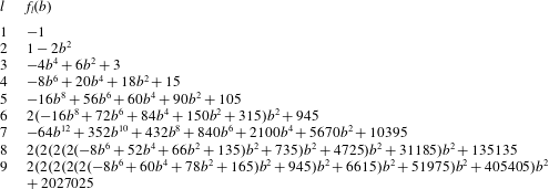
A.1 The case $n=0$

Here, the integral we need to compute is
 $$\begin{eqnarray}\displaystyle \frac{\displaystyle \int \text{d}y\frac{\text{e}^{-y^{2}}}{(y-b)^{2}}}{\displaystyle \int \text{d}yH_{0}^{2}(y)\text{e}^{-y^{2}}}=\frac{{\mathcal{I}}_{0}(b)}{\sqrt{\unicode[STIX]{x03C0}}}.~\Rightarrow ~\left[\frac{\unicode[STIX]{x1D714}^{2}}{\unicode[STIX]{x1D714}_{0}^{2}}-1\right]=\frac{\unicode[STIX]{x1D716}}{a^{2}}+\unicode[STIX]{x1D702}b^{2}\frac{{\mathcal{I}}_{0}(b)}{\sqrt{\unicode[STIX]{x03C0}}}. & & \displaystyle\end{eqnarray}$$
A.2 The case $n=1$

The integral we need to compute is
 $$\begin{eqnarray}\displaystyle \frac{\displaystyle \int \text{d}y{\displaystyle \frac{4y^{2}\text{e}^{-y^{2}}}{(y-b)^{2}}}}{\displaystyle \int \text{d}yH_{1}^{2}(y)\text{e}^{-y^{2}}}=\frac{2{\mathcal{I}}_{1}}{\sqrt{\unicode[STIX]{x03C0}}}=2(b^{2}-1)\frac{{\mathcal{I}}_{0}}{\sqrt{\unicode[STIX]{x03C0}}}-2. & & \displaystyle\end{eqnarray}$$
 Therefore, the dispersion relation for  $n=1$ is given by
 $$\begin{eqnarray}\displaystyle \left[\frac{\unicode[STIX]{x1D714}^{2}}{\unicode[STIX]{x1D714}_{0}^{2}}-1\right]=\frac{3\unicode[STIX]{x1D716}}{a^{2}}+\unicode[STIX]{x1D702}b^{2}\left[2(b^{2}-1)\frac{{\mathcal{I}}_{0}}{\sqrt{\unicode[STIX]{x03C0}}}-2\right]. & & \displaystyle\end{eqnarray}$$
A.3 The case $n=2$

The integral we need to compute is
 $$\begin{eqnarray}\displaystyle \frac{\displaystyle \int \text{d}y\frac{(4y^{2}-2)^{2}\text{e}^{-y^{2}}}{(y-b)^{2}}}{\displaystyle \int \text{d}yH_{2}^{2}(y)\text{e}^{-y^{2}}}=\frac{{\mathcal{I}}_{0}-4{\mathcal{I}}_{1}+4{\mathcal{I}}_{2}}{2\sqrt{\unicode[STIX]{x03C0}}}=3-2b^{2}+[4b^{2}(b^{2}-3)+5]\frac{{\mathcal{I}}_{0}}{2\sqrt{\unicode[STIX]{x03C0}}}.\quad & & \displaystyle\end{eqnarray}$$
 Therefore, the dispersion relation for  $n=2$ is given by
 $$\begin{eqnarray}\displaystyle \left[\frac{\unicode[STIX]{x1D714}^{2}}{\unicode[STIX]{x1D714}_{0}^{2}}-1\right]=\frac{5\unicode[STIX]{x1D716}}{a^{2}}+\unicode[STIX]{x1D702}b^{2}(3-2b^{2})+\unicode[STIX]{x1D702}b^{2}\left[2b^{2}(b^{2}-3)+\frac{5}{2}\right]\frac{{\mathcal{I}}_{0}}{\sqrt{\unicode[STIX]{x03C0}}}. & & \displaystyle\end{eqnarray}$$
A.4 The case $n=3$

The integral we need to compute is
 $$\begin{eqnarray}\displaystyle & & \displaystyle \frac{\displaystyle \int \text{d}y{\displaystyle \frac{(8y^{3}-12y)^{2}\text{e}^{-y^{2}}}{(y-b)^{2}}}}{\displaystyle \int \text{d}yH_{3}^{2}(y)\text{e}^{-y^{2}}}\frac{8{\mathcal{I}}_{3}-24{\mathcal{I}}_{2}+18{\mathcal{I}}_{1}}{6\sqrt{\unicode[STIX]{x03C0}}}\nonumber\\ \displaystyle & & \displaystyle \quad =-\frac{4b^{4}}{3}+6b^{2}-4+[4b^{6}-24b^{4}+33b^{2}-9]\frac{{\mathcal{I}}_{0}}{3\sqrt{\unicode[STIX]{x03C0}}}.\end{eqnarray}$$
 Therefore, the dispersion relation for  $n=3$ is given by
 $$\begin{eqnarray}\displaystyle \left[\frac{\unicode[STIX]{x1D714}^{2}}{\unicode[STIX]{x1D714}_{0}^{2}}-1\right]=\frac{7\unicode[STIX]{x1D716}}{a^{2}}+\unicode[STIX]{x1D702}b^{2}\left(-\frac{4b^{4}}{3}+6b^{2}-4\right)+\unicode[STIX]{x1D702}b^{2}[4b^{6}-24b^{4}+33b^{2}-9]\frac{{\mathcal{I}}_{0}}{3\sqrt{\unicode[STIX]{x03C0}}}.\qquad & & \displaystyle\end{eqnarray}$$
Appendix B. Approximating the integral in (4.8)
To quantitatively evaluate the accuracy of our approximation in (4.9), we can first compute how fast it can recover the normalization as  $n$ increases,
 $$\begin{eqnarray}N=\int H_{n}^{2}(y)\,\text{d}y\text{e}^{-y^{2}}=2^{n}n!\sqrt{\unicode[STIX]{x03C0}}.\end{eqnarray}$$
 To compute the approximate value of this normalization  $N$, as done in § 4.1, we average over the oscillatory part of this approximation first, namely
 $$\begin{eqnarray}\displaystyle {\tilde{N}} & = & \displaystyle 2(2n/e)^{n}\int _{-\sqrt{2n+1}}^{\sqrt{2n+1}}\,\text{d}y\frac{\cos ^{2}\left(y\sqrt{2n+1-{\displaystyle \frac{y^{2}}{3}}}-{\displaystyle \frac{n\unicode[STIX]{x03C0}}{2}}\right)}{\displaystyle \sqrt{1-\frac{y^{2}}{2n+1}}}\nonumber\\ \displaystyle & {\approx} & \displaystyle (2n/e)^{n}\int _{-\sqrt{2n+1}}^{\sqrt{2n+1}}\frac{\text{d}y}{\sqrt{1-{\displaystyle \frac{y^{2}}{2n+1}}}}\nonumber\\ \displaystyle & = & \displaystyle \unicode[STIX]{x03C0}\sqrt{2n+1}\left(\frac{2n}{\exp (1)}\right)^{n}.\end{eqnarray}$$
Therefore, the error in the normalization due to our approximation is given by
 $$\begin{eqnarray}\displaystyle N_{r}\equiv \frac{{\tilde{N}}-N}{N}=\frac{\text{e}^{-n}n^{n}\sqrt{\unicode[STIX]{x03C0}(2n+1)}}{n!}-1. & & \displaystyle\end{eqnarray}$$
 On the left-hand side of figure 5, we plot the error  $N_{r}$ as a function of the Hermite index $n$. This shows that our approximation produces a relative error of less that 1 % for $n>20$.
However, when we compute the dispersion relation, the largest error in the integral comes from the difference between the analytical and approximate forms near the poles, i.e. near the solutions. Therefore, we compare the values of the integral and its approximation near the expected solution. The integral in (4.8) is
 $$\begin{eqnarray}\displaystyle I_{1}(b,n)=\frac{1}{\displaystyle \int \text{d}yH_{n}^{2}(y)\text{e}^{-y^{2}}}\int \text{d}y\frac{H_{n}^{2}(y)\text{e}^{-y^{2}}}{(y-b)^{2}}=\frac{1}{\sqrt{\unicode[STIX]{x03C0}}2^{n}n!}\int _{-\infty }^{\infty }\,\text{d}y\frac{H_{n}^{2}(y)\text{e}^{-y^{2}}}{(y-b)^{2}}. & & \displaystyle\end{eqnarray}$$
This is approximated by
 $$\begin{eqnarray}\displaystyle I_{2}(b,n) & = & \displaystyle \frac{\displaystyle \int _{-\sqrt{2n+1}}^{\sqrt{2n+1}}\,\text{d}y\left[1-\frac{y^{2}}{2n+1}\right]^{-1/2}(y-b)^{-2}}{\displaystyle \int _{-\sqrt{2n+1}}^{\sqrt{2n+1}}\,\text{d}y\left[1-\frac{y^{2}}{2n+1}\right]^{-1/2}}=\frac{1}{2n+1}\frac{\displaystyle \int _{-1}^{1}\,\text{d}z\frac{[1-z^{2}]^{-1/2}}{(z-b/\sqrt{2n+1})^{2}}}{\displaystyle \int _{-1}^{1}\text{d}z[1-z^{2}]^{-1/2}}\nonumber\\ \displaystyle & = & \displaystyle \frac{b}{(b^{2}-(2n+1))^{3/2}},\end{eqnarray}$$
 where we assumed that  $\mathtt{Im}(b)\neq 0$. Before comparing the values of the two functions, $I_{1}$ and $I_{2}$, for different values of $n$, we first need to compute the characteristic value of their complex and dimensionless argument, $b$, that enables a meaningful comparison. Using
 $$\begin{eqnarray}\displaystyle b^{2} & \equiv & \displaystyle \frac{\unicode[STIX]{x1D714}^{2}}{a^{2}v_{b}^{2}}=\frac{\unicode[STIX]{x1D714}^{2}}{\unicode[STIX]{x1D714}_{0}^{2}}\frac{\unicode[STIX]{x1D714}_{0}^{2}}{v_{b}^{2}}\sqrt{\frac{3}{\unicode[STIX]{x1D716}}}\frac{\unicode[STIX]{x1D70E}}{\unicode[STIX]{x1D714}_{0}}=\frac{\unicode[STIX]{x1D714}^{2}}{\unicode[STIX]{x1D714}_{0}^{2}}\frac{\unicode[STIX]{x1D70E}^{2}}{v_{b}^{2}}\sqrt{\frac{3}{\unicode[STIX]{x1D716}\unicode[STIX]{x1D706}_{D}}}\sim \frac{\unicode[STIX]{x1D714}^{2}}{\unicode[STIX]{x1D714}_{0}^{2}}(2n_{m}+1)\nonumber\\ \displaystyle & \Rightarrow & \displaystyle \mathtt{Re}(b)\sim \sqrt{2n_{m}+1}~\& ~\mathtt{Im}(b)\sim \unicode[STIX]{x1D702}^{2/5}\mathtt{Re}(b).\end{eqnarray}$$
We show in figure 5(b) the dependence of the relative error, i.e.  $(I_{2}-I_{1})/I_{1}$, on the value of $n_{m}$ for $\unicode[STIX]{x1D702}=10^{-5}$. Figure 5(b) shows that the error in the approximation of the integral decreases as the value of $n_{m}$ increases. The error in the imaginary part of the integral (which dictates the value of the growth rates) is the smallest error and decreases exponentially fast. This establishes the validity of our approximation of the integral to compute the fastest growth rate in the large- $n$ limit.
(a) The dependence of the normalization error,  $N_{r}$ of (B 3), on the value of Hermite index $n$. (b) The dependence of the relative error, i.e. $(I_{2}-I_{1})/I_{1}$, on the value of $n_{m}$ with $\mathtt{Re}(b)=\sqrt{2n_{m}+1}$ and $\mathtt{Im}(b)=\unicode[STIX]{x1D702}^{2/5}\mathtt{Re}(b)$, with $\unicode[STIX]{x1D702}=10^{-5}$. The relative error in the approximate integral is a complex function. Thus, we compare the error in the real part (red), the imaginary part (blue) and the absolute value (green).


