1. Introduction

A physical and theoretical understanding of the rheological behaviour of ice has long been the quest of glaciologists. It is fundamental to understanding how glaciers and ice sheets flow, and represents a major component of ice velocity in many ice masses. It is of great importance that we can model accurately the flow of glaciers and ice sheets and smaller ice bodies of the world, through the past, to the present and into the future.

At present, Glen’s flow law provides an adequate description of steady-state ice deformation for most applications (Reference GlenGlen, 1955). It relates the strain rate, thus:

(1)

where A is a constant related to temperature, grain morphology, liquid H₂O content and hydrostatic head, and has values between 10^–14 and 10^–21 s^–1 kPa^–3 (Reference PatersonPaterson, 1994), τ_xz is the longditudinal component of the shear stress (where z is perpendicular and × is parallel to the surface slope) and n is a constant whose value is approximately 3.0 with a range of approximately 2–4 (Reference Weertman, Whalley, Jones and GoldWeertman, 1973).

However, transient creep is a significant factor both in laboratory tests which are designed to parameterize Equation (1) and in small ice bodies such as cirque glaciers and active rock glaciers whose ice residence time is of the same order of magnitude as the transient effects. Thus, a more general description of the rheology would combine Equation (1) with a transient creep component, ε_T, thus:

(2)

where ε_E is an instantaneous elastic response and is the steady-state (secondary) creep rate.

The transient component can be modelled using a term in which decays to zero at t = ∞ (viscoelastic) of the form:

(3)

where B = (1 + v)/2E _Young and τ_R is a relaxation time which depends upon various material properties. Another way of describing the transient creep component uses a power-law dependency (Reference Azizi, Whalley, Chung, Sayed and GresnigtAzizi and Whalley, 1995) of the form

(4)

where A and m are creep parameters, A being the same as that used in Equation (1).

Clearly, where m = 0, steady-state conditions apply, and where m = 1, accelerating (tertiary) creep is assumed.

Such transient effects dominate the behaviour of small ice bodies in their initial stages. Reconstructions of the dynamics of small ice bodies such as alpine rock glaciers (Reference KääbKääb, 1996) have used steady-state rheologies for simplicity. However, the importance of the transient creep effects has been demonstrated by Reference Azizi, Whalley, Chung, Sayed and GresnigtAzizi and Whalley (1995), although parameterization of such effects remains problematic. Field sociologists have known for a long time that ice character varies markedly in real ice masses, especially within the lower ˚basal ice" layers of glaciers (Reference Kamb and LaChapelleKamb and LaChapelle, 1964; Reference LawsonLawson, 1979; Reference KnightKnight, 1997) and within the deforming zones of alpine rock glaciers (Reference Vonder Muhll and HolubVonder Mühll and Holub, 1992). Intuitively, rheological variability must occur as a result of the differences in the physical character of ice found throughout ice masses but most profoundly within the lower basal ice layers. Experimental and field observations have supported this (Reference SwinzowSwinzow, 1962; Reference Kamb and LaChapelleKamb and LaChapelle, 1964; Reference Kamb and ShreveKamb and Shreve, 1966; Reference Goughnour and AnderslandGoughnour and Andersland, 1968; Reference Hooke, Dahlin and KauperHooke and others, 1972; Reference Echelmeyer and ZhongxiangEchelmeyer and Wang, 1987; Reference PatersonPaterson, 1994). These rheological variations have not yet been incorporated into any glacier flow models, and there are at least three major reasons for this:

Further work is required to improve the applicability of the flow law through better parameterization. At present, studies of ice deformation are conducted by the instrumentation of either a natural feature in situ or small samples considered representative of that feature exposed to an artificial stress regime (Reference Barnes, Tabor and WalkerBarnes and others, 1971; Reference Hooke, Dahlin and KauperHooke and others, 1972; Reference BakerBaker, 1978; Reference Duval, Ashby and AndermanDuval and others, 1983; Reference Jacka, Budd, Jones, McKenna, Tillot-son and JordaanJacka and Budd, 1991). The difficulty associated with field-based investigations (including the often harsh conditions under which such measurements are made) obviously points towards a laboratory-based approach being very useful and one which must be utilized. Until now, laboratory-based physical modelling has been limited to the application of uniform stress fields to samples, with stress being varied in incremental steps. This forces the extrapolation from discretized, small-scale, test samples through a piece-wise superposition, up to realistic scales. However, the stress gradient acting through an ice mass (referred to in engineering terms as prototype) is a function of gravitational potential as described by Newton’s second law (F = ma). The steady-state deformation response of ice is non-linear, following a power-law flow relation, whereby the rate of deformation is proportional to a value between the second and fourth powers of the applied stress (Equation (1)). The most effective way to physically model the non-linear aspects of ice deformation would be to apply a non-uniform stress field to a sample, and the continuous function described by Equation (2) can then be better parameterized to describe the deformation. In the prototype the stress gradient is the product of ice density, ice thickness and gravity and so can be replicated in a model ice sample by exposing the sample to an enhanced gravity field. This can be achieved by flying samples of ice in a geotechnical beam centrifuge. In the following sections we shall introduce the concept of centrifuge modelling, the scaling laws associated with it and the results from two tests on isotropic polycrystalline ice.

2. Geotechnical Centrifuges: Theory

The geotechnical beam centrifuge is a unique physical modelling tool, the "power"of which has been known to geotechnical engineers for some years, but is only now gaining a profile in Earth Sciences. In many earth surface phenomena the role of self-weight body forces is crucial in explaining observed behaviour, i.e. where in situ stresses change with depth and the response of the material may alter in response to these stress differences. As suggested above, the best way to model physically ice deformation is to replicate the self-weight stress gradient experienced in Nature within the model as a continuous function. A scale model fixed onto the end of a centrifuge arm which is then rotated ("flown") rapidly experiences ˚an inertial radial acceleration field which, as far as the model is concerned, feels like a gravitational acceleration field but many times stronger than Earth’s gravity field" (Reference Taylor and TaylorTaylor, 1995). The model experiences zero stress at the surface (in our models this is the surface of the overburden steel plate), but this increases with depth, producing a stress gradient that is directly comparable to that experienced in field prototypes.

2.1. Scaling

Certain scaling issues must be addressed for the various time-dependent and time-independent processes, in order to relate the model to the prototype.

2.11 Linear dimensions

If a scale model of the field prototype (Fig. 1) is subjected to an inertial acceleration field which is N times Earth’s gravity, then at model depth h_m, the vertical stress in the model, s, is:

(5)

The same stress occurs in the prototype where σ_zp = σ_zm, so the depth of the homologous point can be calculated as:

(6)

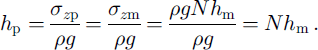
Hence, the scaling relationship for macroscopic linear dimensions is 1: N. Problems can potentially arise with understress being experienced towards the top surface of the model, and overstress at its base, due to the proportional relationship between radial acceleration (a) and distance from the axis of rotation (r) a = ω ² r, where ω is the angular rotational speed of the centrifuge. This error was calculated to be ≤ 2% for the model geometry used herein (Reference IrvingIrving, 2000).

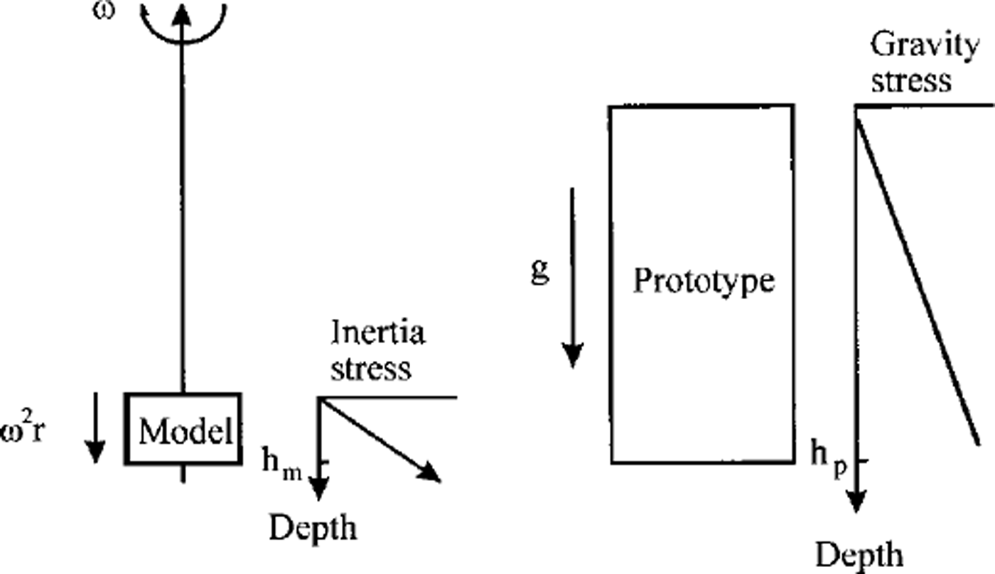
Fig. 1. The correspondence of inertial stresses generated in a centrifuge model to those in prototype (Nature).

2.1.2. Grain-size and temperature

Equation (6) is applicable over macroscopic length scales only. However, a continuous flow-law function treats the sample as both a continuum and (via A), a collection of par-tides. This is problematic in that the interactions between the ice grains are many and complex, occurring through processes which are both diffusive and translative. The latter processes will scale as 1:1. There is much uncertainty over the diffusive processes, but recent research estimates the relationship to be in the range 1: N² to 1: N³ (Reference IrvingIrving, 2000). In this experiment:

D is a significant fraction of sample thickness (8 mm ≤ D ≤ 10 mm in a sample 180 mm thick), in order to satisfy the assumption of purely macroscopic (dislocation) interaction between grains

the temperature is below –3.5°C. An Arrhenius-type viscosity relationship is not assumed (Reference Mellor and TestaMellor and Testa, 1969).

However, empirically derived values for A are well constrained for power-law creep at this temperature (Irving, 1999). The tests were of a short enough duration, with small strains, that physico-chemical interactions leading to re-crystalhzation were negligible.

2.1.3. Creep

The discipline of centrifuge modelling is still relatively new, having only really developed in earnest since the early 1970s. It has been very much the realm of the geotechnical engineer, so the scaling laws have been developed only in areas which are of interest to engineers. Gold-regions centrifuge studies have been restricted to geotechnical tests on permafrost (Reference Ketcham and BlackKetcham and Black, 1995; Reference Harris, Rea and DaviesHarris and others, 2000) mainly related to thawing and consolidation processes. A limited amount of work has been done on the modelling of sea-ice-structure interactions, with the ice actually being formed during flight at enhanced g levels (e.g. Reference Lovell, Schofield, Murthy, Connor and BrebbiaLovell and Scholfield, 1986). Centrifuge modelling of the creep of frozen soils has received little attention, and no data exist on the potential time-scaling of ice creep. Time-scaling for creep will lie somewhere between 1:1 and 1: N ³, and Reference Smith and TaylorSmith (1995) suggests that, because stresses and temperatures are identical between the model and the prototype, scaling should be 1:1. This, however, ˚has not been experimentally demonstrated" Reference Smith and Taylor(Smith, 1995). Time may scale by N ² if crystal sizes are reduced by N for a pure ice sample. However, a reduction in grain-size by a factor of N will lead to an alteration in the dominant creep mechanism from power-law to diffusion. This could then lead to the modelling of non-power-law creep. The data obtained from these tests should allow the first comprehensive conclusions of time-scaling for ˚pure" ice creep in centrifuge modelling. The time-scaling for creep is explored further below.

3. Method

The aim of this research project was to establish the potential for modelling polycrystalline-ice deformation using the geotechnical centrifuge. In order to minimize our centrifuge testing time (by maximizing strain rate) and to model ˚realistic" ice thicknesses, we decided to attempt to replicate the deformation in a 50 m thick glacier. To reduce the errors (from over- and understressing due to differences in r), models have been made thin and loaded with plate-steel overburden which, having a density 7.85 times that of ice, reduces the overall model thickness substantially. Thus, only the lower part of the glacier is modelled, which is acceptable since shear stress and hence strain are concentrated here as described by Equation (1).

3.1. Test-bed configuration

3.11 Test box

The test-bed design is shown in Figure 2 and described in detail in Reference IrvingIrving (2000). A slope of 15° was calculated as the optimum for maximizing the strain rate while utilizing the full dimensions of the box. (A basal shear stress of 106 kPa was developed at the bottom of the model.) The two ice models were placed side by side in the strongbox. It was assumed that with the expected strains for such a short test duration there would be negligible mechanical coupling between the two samples. The outward-facing sides of the samples were confined by the Perspex walls of the test box. Deformation can therefore be treated as simple shear. Models were unconfined on their downslope end.

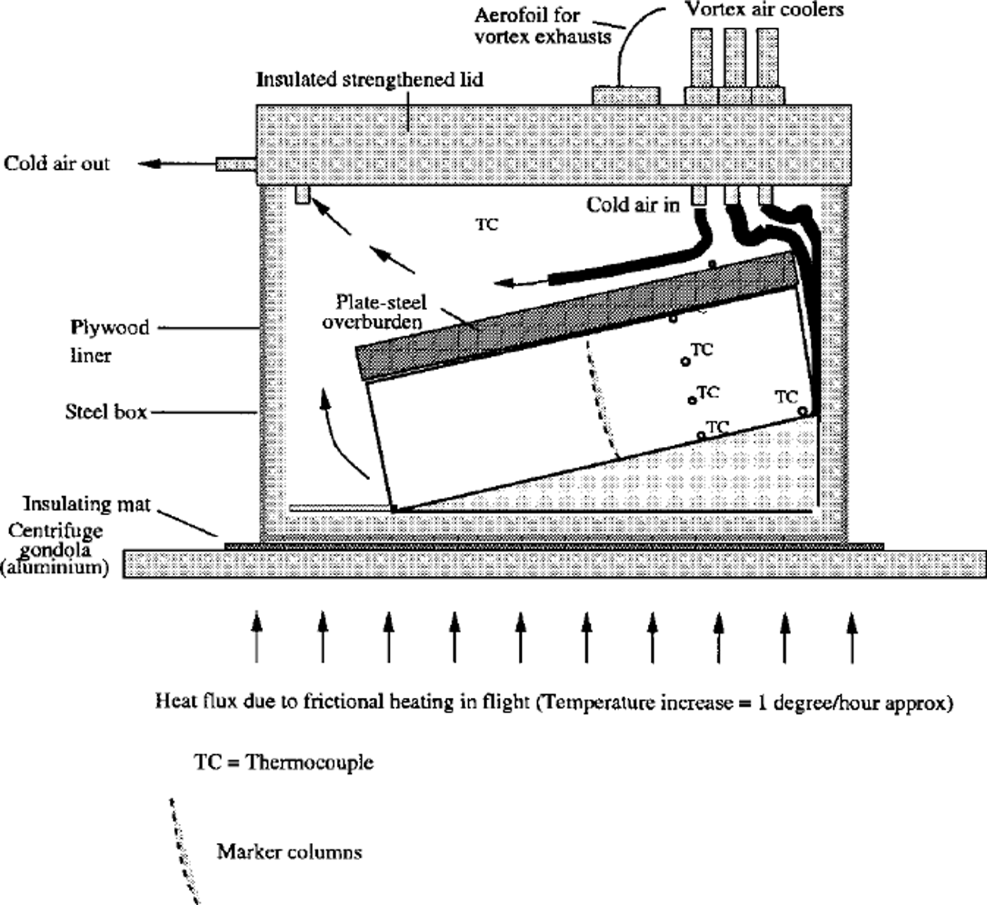
Fig. 2. The strongbox design, with cooling system and models in place.

3.1.2. Cooling system

To maintain thermal equilibrium during testing, three MEECH-ARTEX vortex tubes were used to cool the strongbox. Each vortex tube is capable of generating an air stream at –20°C with a flow rate of 220 L mirT¹. One tube was directed below the base-plate of each model, and the third was passed into the upper void space above the models. Models were insulated along the base and ends by 25 mm plywood, and the top enclosed by an insulating lid (Fig. 2).

However, heat removal by these air streams was not sufficient to balance the rate of heat transferral to the test-bed due to the motion of the centrifuge arm (175 km IT¹) through the air mass in the centrifuge pit. At best, temperature could be maintained at approximately –7°C for an initial period of approximately 30 min and then rose gradually during the remainder of the test to –1°C over a 5 hour flight. The test would then be paused for 12–18 hours to return the model to a lower temperature. Models remained on the arm in the centrifuge pit and were cooled by the vortex tubes.

3.1.3 Instrumentation

The instrumentation for each model comprised an array of K-type thermocouples, four columns of deformation markers in each sample and a video camera to monitor the time development of strain during the test. No data were collected from the video camera, due to technical difficulties, and thermal data were likewise not recorded for the final 5 hours of the test series.

4. Results

As continuous strain data were not recorded, we cannot quantify the rate of decay of transient creep. Maximum measured displacements at 12 cm from the bed are: for model la, 9.54 mm; for model lb along the centre line, 6 mm; and at the edge of the model in contact with the Perspex side-wall, 4.2 mm.

With reference to Figure 3, the final deformation is interpreted for each recovered column of markers.

Fig. 3. Deformation profiles from columns la-3 (a), lb-1 (b), lb-2 (c) and 3–3 (d) (solid curved line), along with the viscoelastic approximation (solid line) and the visco-plastic approximation (dashed line).

1a-3, centre line, halfway downslope

1b-1, outer edge, halfway downslope

1b-2, centre line, one-third distance downslope

1b-3, centre line, halfway downslope

5. Analysis

The deformation data were converted to a shear strain making the following assumptions:

The incremental shear strain, ε = tanβ (where /3 is the ice-surface slope), was calculated as the ratio of marker downslope displacement, d, to marker spacing, h:

(7)

This was converted to a strain rate, by dividing by the total time over which the models were subjected to an acceleration of 80g, t = 52 200 s. Some markers were disturbed during exhumation, so the displacement curves are not as smooth as would be expected. The expected strain for each displacement marker was then calculated using both Equations (2) and (4). No instantaneous strain component in Equation (2) was observed, and its effect is not considered in this analysis.

Equations (2) and (4) were parameterized using reasonable values for A, B, n, τ_R and m. A least-squares regression was performed to fit the generated curves from Equations (2) and (4) to the strain curves measured from the models. The predicted deformation from both of the models is plotted in Figure 3, with the viscoelastic transient component predicting greater deformation at depth than the visco-plastic transient component, while the reverse is the case in the upper regions of the models.

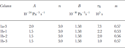
Whilst the fitted curves describe the observed deformation well in the lower regions of the models, the departure in the upper regions occurs because both equations are highly sensitive to shear stress. It is a goodness of fit in the lower regions which is most desirable. The best-fit parameters for each model for each descriptive equation are shown in Table 1.

Table 1. Best-fit parameters for A B, n, τ _R and mused in the viscoelastic and visco-plastic approximations (see Fig 3)

6. Discussion

The material properties of the the two models were similar except for the stratigraphic differences within model la. The effect of this layering was to reduce the relaxation time, τ_R, which would be expected given that a zone with a lower bulk density will store less elastic strain. However, the magnitude of τ_R in both models is several orders greater than other reported values (Reference Jellinek and BrillJellinek and Brill, 1956) which are typically 100–1000 s for stresses and temperatures similar to those in the tests described above. It is suggested that this is due to scaling. If there is indeed a scaling relationship between the diffusive (and hence microscopic-scale) processes that lies at the upper end of the range suggested in section 2.1, then the relaxation time proposed in Table 1 for a model in the centrifuge is reasonable. Comparing the values obtained in Table 1 with the values obtained by Reference Jellinek and BrillJelli-nek and Brill (1956) suggests an approximate scaling of 1: JV¹⁷ with time. Whilst the accuracy of this value is open to debate, it closes the range of probable values by a factor of N to somewhere between 1: N and 1: N³.

The issue of grain-size scaling is worth addressing briefly. If grain-size is reduced by a factor N, then Reference Smith and TaylorSmith (1995) suggested that time would scale with 1: N². As mentioned previously Reference Duval, Ashby and AndermanDuval and others (1983) stated that a reduction in grain-size to 1 mm for polycrystalline-ice samples will result in diffusive processes becoming the dominant mechanism of creep. A reduction of crystal size by N in our samples could result in models creeping by diffusive rather than dislocation processes. Thus, for these initial tests crystal sizes were not scaled down. We have not incorporated a grain-size reduction into our calculations, but, as is implied by the treatment arising from Equations (3) and (4), there is a significant effect arising from the microscopic processes which would serve to skew the scaling from an expected 1:1 relationship for purely dislocational processes. This may well explain the intermediate value arrived at above.

7. Conclusions

The application of a stress gradient to a sample is intuitively the best method for modelling ice-deformation processes in the laboratory. From the evidence presented above it is clear that this can be successfully undertaken using ice models in a geotechnical beam centrifuge. Additional steel overburden can be added to the upper surface of models in order to increase the normal and basal shear stresses to a level that would be experienced at the bed of some valley glaciers or rock glaciers.