


1. Introduction
The energy cascade, which describes the transfer of kinetic energy from the largest scales of fluid motion to smaller scales until it is eventually converted to heat by viscous dissipation, is a central principle of turbulence theory (Richardson Reference Richardson1926; Kolmogorov Reference Kolmogorov1941a ). In freely decaying homogeneous isotropic turbulence, the dissipation of turbulent kinetic energy (TKE) simplifies to
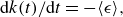 \begin{equation} \textrm{d}k(t)/\textrm{d}t = -\langle \epsilon \rangle , \end{equation}
where $\langle \epsilon \rangle$
is the ensemble-averaged dissipation, and
$\langle \epsilon \rangle$
is the ensemble-averaged dissipation, and $k(t)= ({1}/{2})\langle u_iu_i \rangle$
is the TKE, with
$k(t)= ({1}/{2})\langle u_iu_i \rangle$
is the TKE, with $u_i$
being fluctuating velocity components (Pope Reference Pope2000). However, there is no exact solution for this simple equation as the relationship between
$u_i$
being fluctuating velocity components (Pope Reference Pope2000). However, there is no exact solution for this simple equation as the relationship between $\langle \epsilon \rangle$
and
$\langle \epsilon \rangle$
and $u_i$
or
$u_i$
or $k$
is not known a priori.
$k$
is not known a priori.
However, it is well established that the decay of kinetic energy of freely decaying homogeneous isotropic turbulence is self-similar and follows a power law in time of the form $k(t)\propto t^{-n}$
. The decay in
$k(t)\propto t^{-n}$
. The decay in $k$
is accompanied by the growth of the integral length scale
$k$
is accompanied by the growth of the integral length scale $L$
, which also follows a power law,
$L$
, which also follows a power law, $L(t)\propto t^m$
. There are two well-known theoretical predictions for
$L(t)\propto t^m$
. There are two well-known theoretical predictions for $n$
and
$n$
and $m$
based on the assumption that the turbulence should contain some invariants of motion. Considering the conservation of angular momentum (Loitsiansky’s integral) yields
$m$
based on the assumption that the turbulence should contain some invariants of motion. Considering the conservation of angular momentum (Loitsiansky’s integral) yields $k\propto t^{-10/7}$
and
$k\propto t^{-10/7}$
and $L\propto t^{2/7}$
(Kolmogorov Reference Kolmogorov1941b
), while considering the conservation of linear momentum results in
$L\propto t^{2/7}$
(Kolmogorov Reference Kolmogorov1941b
), while considering the conservation of linear momentum results in $k\propto t^{-6/5}$
and
$k\propto t^{-6/5}$
and $L\propto t^{2/5}$
(Birkhoff Reference Birkhoff1954; Saffman Reference Saffman1967). Early studies of grid turbulence by Batchelor & Townsend (Reference Batchelor and Townsend1948) and Comte-Bellot & Corrsin (Reference Comte-Bellot and Corrsin1966) verified the power-law scaling, after an initial transition period close to the grid, finding that values of
$L\propto t^{2/5}$
(Birkhoff Reference Birkhoff1954; Saffman Reference Saffman1967). Early studies of grid turbulence by Batchelor & Townsend (Reference Batchelor and Townsend1948) and Comte-Bellot & Corrsin (Reference Comte-Bellot and Corrsin1966) verified the power-law scaling, after an initial transition period close to the grid, finding that values of $n$
varied in the range
$n$
varied in the range $1.15\leqslant n \leqslant 1.29$
. Many grid turbulence studies have been carried out since, including Hak & Corrsin (Reference Hak and Corrsin1974), Warhaft & Lumley (Reference Warhaft and Lumley1978), Lavoie & Antonia (Reference Lavoie, Djenedi and Antonia2007), Krogstad & Davidson (Reference Krogstad and Davidson2009) and Sinhuber et al. (Reference Sinhuber, Bodenschatz and Bewley2015), to name a few, and have reported values of
$1.15\leqslant n \leqslant 1.29$
. Many grid turbulence studies have been carried out since, including Hak & Corrsin (Reference Hak and Corrsin1974), Warhaft & Lumley (Reference Warhaft and Lumley1978), Lavoie & Antonia (Reference Lavoie, Djenedi and Antonia2007), Krogstad & Davidson (Reference Krogstad and Davidson2009) and Sinhuber et al. (Reference Sinhuber, Bodenschatz and Bewley2015), to name a few, and have reported values of $n$
close to both thoeretical predictions. More recent studies by Hurst & Vassilicos (Reference Hurst and Vassilicos2007), Krogstad & Davidson (Reference Krogstad and Davidson2011), Valente & Vassilicos (Reference Valente and Vassilicos2011) and Hearst & Lavoie (Reference Hearst and Lavoie2014) have examined turbulence produced by complex grids, such as fractal or multi-scale grids, which have also been found to exhibit similar values of
$n$
close to both thoeretical predictions. More recent studies by Hurst & Vassilicos (Reference Hurst and Vassilicos2007), Krogstad & Davidson (Reference Krogstad and Davidson2011), Valente & Vassilicos (Reference Valente and Vassilicos2011) and Hearst & Lavoie (Reference Hearst and Lavoie2014) have examined turbulence produced by complex grids, such as fractal or multi-scale grids, which have also been found to exhibit similar values of $n$
in the far field. Overall, there is no conclusive evidence supporting
$n$
in the far field. Overall, there is no conclusive evidence supporting $n=10/7$
or
$n=10/7$
or $6/5$
, but there appears to be broad agreement that the values of
$6/5$
, but there appears to be broad agreement that the values of $n$
vary in the range
$n$
vary in the range $1\leqslant n \leqslant 1.6$
.
$1\leqslant n \leqslant 1.6$
.
The physical size of the facility can also affect the turbulent decay rate due to the continuous growth of the integral length scale to saturation, increasing values of $n\rightarrow 2$
or greater (Smith et al. Reference Smith, Donnelly, Goldenfeld and Vinen1993; Skrbek & Stalp Reference Skrbek and Stalp2000; Hwang & Eaton Reference Hwang and Eaton2004; Esteban et al. Reference Esteban, Shrimpton and Ganapathisubramani2019; Panickacheril John et al. Reference Panickacheril John, Donzis and Sreenivasan2022). Exemplary examples of saturation are found in the towed grid study by Smith et al. (Reference Smith, Donnelly, Goldenfeld and Vinen1993) and box turbulence by Hwang & Eaton (Reference Hwang and Eaton2004) and Esteban et al. (Reference Esteban, Shrimpton and Ganapathisubramani2019). These high values of
$n\rightarrow 2$
or greater (Smith et al. Reference Smith, Donnelly, Goldenfeld and Vinen1993; Skrbek & Stalp Reference Skrbek and Stalp2000; Hwang & Eaton Reference Hwang and Eaton2004; Esteban et al. Reference Esteban, Shrimpton and Ganapathisubramani2019; Panickacheril John et al. Reference Panickacheril John, Donzis and Sreenivasan2022). Exemplary examples of saturation are found in the towed grid study by Smith et al. (Reference Smith, Donnelly, Goldenfeld and Vinen1993) and box turbulence by Hwang & Eaton (Reference Hwang and Eaton2004) and Esteban et al. (Reference Esteban, Shrimpton and Ganapathisubramani2019). These high values of $n$
observed in experiments have also been derived by invoking scaling arguments. Lohse (Reference Lohse1994) derived expressions for the dimensionless energy dissipation rate based on different Reynolds number scalings,
$n$
observed in experiments have also been derived by invoking scaling arguments. Lohse (Reference Lohse1994) derived expressions for the dimensionless energy dissipation rate based on different Reynolds number scalings, $Re$
and
$Re$
and $Re_{\lambda }$
, which captured the decay rate of mean vorticity observed in the towed grid experiments of Smith et al. (Reference Smith, Donnelly, Goldenfeld and Vinen1993). Using a similar approach, Panickacheril John et al. (Reference Panickacheril John, Donzis and Sreenivasan2022) also used the mean energy dissipation
$Re_{\lambda }$
, which captured the decay rate of mean vorticity observed in the towed grid experiments of Smith et al. (Reference Smith, Donnelly, Goldenfeld and Vinen1993). Using a similar approach, Panickacheril John et al. (Reference Panickacheril John, Donzis and Sreenivasan2022) also used the mean energy dissipation $\langle \epsilon \rangle =C_{\epsilon }\,\mathcal{U}^{3}/\mathcal{L}$
, where
$\langle \epsilon \rangle =C_{\epsilon }\,\mathcal{U}^{3}/\mathcal{L}$
, where $\mathcal{U}$
and
$\mathcal{U}$
and $\mathcal{L}$
are the velocity and length scales characteristic of the energy injection, and
$\mathcal{L}$
are the velocity and length scales characteristic of the energy injection, and $C_{\epsilon }$
is a constant, to show that the decay in a confined turbulent flow varies as
$C_{\epsilon }$
is a constant, to show that the decay in a confined turbulent flow varies as $k(t)\propto t^{-2}$
. This is in contrast to the self-similarity argument of freely decaying turbulence that leads to
$k(t)\propto t^{-2}$
. This is in contrast to the self-similarity argument of freely decaying turbulence that leads to $k(t)\propto t^{-1}$
(Batchelor Reference Batchelor1953). We emphasise the difference between the final period of decay and saturation. The former is associated only with very low Reynolds numbers, while the latter can happen at any Reynolds number, depending on the size of the facility.
$k(t)\propto t^{-1}$
(Batchelor Reference Batchelor1953). We emphasise the difference between the final period of decay and saturation. The former is associated only with very low Reynolds numbers, while the latter can happen at any Reynolds number, depending on the size of the facility.
Measurements of turbulent decay within closed vessels are comparatively fewer than grid turbulence in wind tunnels or water channels (Hwang & Eaton Reference Hwang and Eaton2004; Verschoof et al. Reference Verschoof, Huisman, van der Veen, Sun and Lohse2016; Ostilla-Mónico et al. Reference Ostilla-Mónico, Verzicco, Grossmann and Lohse2014, Reference Ostilla-Mónico, Lohse and Verzicco2016, Reference Ostilla-Mónico, Zhu, Spandan, Verzicco and Lohse2017; Esteban et al. Reference Esteban, Shrimpton and Ganapathisubramani2019). A recent study by Esteban et al. (Reference Esteban, Shrimpton and Ganapathisubramani2019) investigated the temporal decay of homogeneous anisotropic turbulence generated in a box by a random jet array with zero mean flow, and reported the evolution of $n$
. They observed a decay exponent
$n$
. They observed a decay exponent $n=2.3$
during the initial period typical of values in the near-field region of grid turbulence, which reduced to
$n=2.3$
during the initial period typical of values in the near-field region of grid turbulence, which reduced to $n=1.4$
, which is close to
$n=1.4$
, which is close to $10/7$
and similar to values found in the far-field region of grid turbulence. After some time, the final decay regime emerged with decay exponent
$10/7$
and similar to values found in the far-field region of grid turbulence. After some time, the final decay regime emerged with decay exponent $n=1.8$
due to saturation as the growth of the integral length scale approaches the size of the box. A similarly high value
$n=1.8$
due to saturation as the growth of the integral length scale approaches the size of the box. A similarly high value $n=1.86$
was reported by Hwang & Eaton (Reference Hwang and Eaton2004) for the same reasons.
$n=1.86$
was reported by Hwang & Eaton (Reference Hwang and Eaton2004) for the same reasons.
In this paper, we present measurements of the decay of high Reynolds number stationary turbulence in a von Kármán flow. This configuration produces a large turbulent shear flow at the midplane between two counter-rotating impellers within a closed cylindrical vessel, and has been a subject of interest in turbulence research since the original work of Batchelor (Reference Batchelor1951), Stewartson (Reference Stewartson1953), Picha & Eckert (Reference Picha and Eckert1958) and Zandbergen & Dijkstra (Reference Zandbergen and Dijkstra1987). Von Kármán flows have been particularly well suited to the experimental study of the structure and dynamics of small-scale turbulence due to their ability to produce high Reynolds number homogeneous turbulent fluctuations in the central region of the vessel, as demonstrated by Ouellette et al. (Reference Ouellette, Xu, Bourgoin and Bodenschatz2006), Worth & Nickels (Reference Worth and Nickels2011), Lawson & Dawson (Reference Lawson and Dawson2015), Huck et al. (Reference Huck, Machicoane and Volk2017), Knutsen et al. (Reference Knutsen, Baj, Lawson, Bodenschatz, Dawson and Worth2020), Debue et al. (Reference Debue, Valori, Cuvier, Daviaud, Foucaut, Laval, Wiertel, Padilla and Dubrulle2021) and Aligolzadeh et al. (Reference Aligolzadeh, Holzner and Dawson2023) to name but a few. However, to the best of the authors’ knowledge, no measurements of turbulent decay have yet been reported in von Kármán flows.
To address this gap, the decay of TKE of the velocity fluctuations at Reynolds numbers based on the Taylor microscale ( $\lambda$
) of
$\lambda$
) of $Re_{\lambda }=493, 599, 689$
produced in a von Kármán flow was investigated using stereoscopic particle image velocimetry (PIV). Access to all three velocity components allows for separate and cumulative analysis of the decay rates. Measurements of the turbulent decay begin immediately after abruptly stopping the impellers, and continue for 10, 15 or 20 impeller revolution periods, depending on the initial rotation speed. We introduce a fitting function based on a one-dimensional energy spectrum to determine the evolution of the decay exponent, which includes an initial transition phase where the TKE remains constant for a short time after the impellers are stopped due to inertia. Evidence is also presented of a large-scale inversion of the flow before the onset of the turbulent decay rate.
$Re_{\lambda }=493, 599, 689$
produced in a von Kármán flow was investigated using stereoscopic particle image velocimetry (PIV). Access to all three velocity components allows for separate and cumulative analysis of the decay rates. Measurements of the turbulent decay begin immediately after abruptly stopping the impellers, and continue for 10, 15 or 20 impeller revolution periods, depending on the initial rotation speed. We introduce a fitting function based on a one-dimensional energy spectrum to determine the evolution of the decay exponent, which includes an initial transition phase where the TKE remains constant for a short time after the impellers are stopped due to inertia. Evidence is also presented of a large-scale inversion of the flow before the onset of the turbulent decay rate.
2. Experiments
2.1. Apparatus and measurements
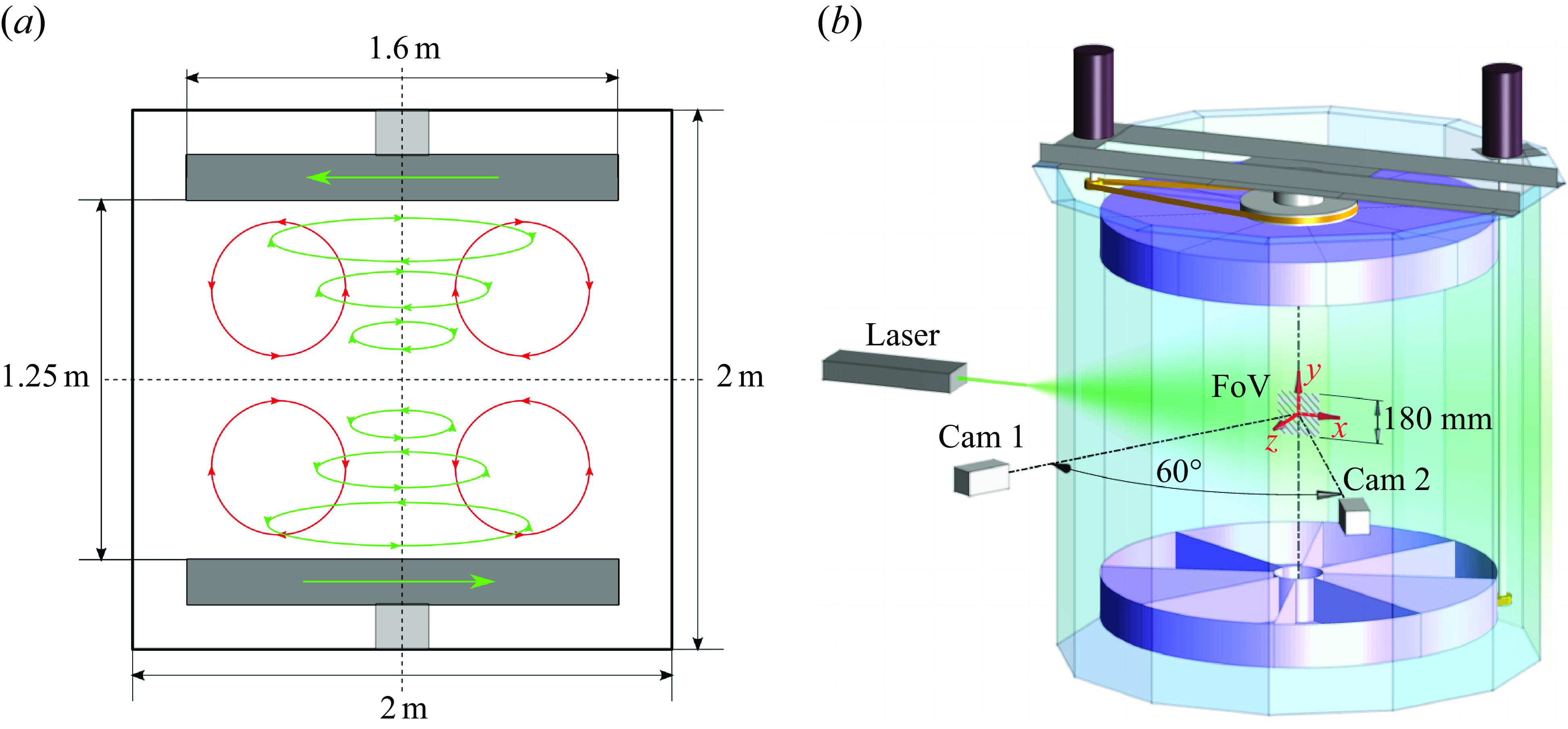
Experiments were carried out in a large dodecagonal Perspex water tank which is $2$
m high with radius
$2$
m high with radius $1$
m, as shown in figure 1. Two counter-rotating impellers,
$1$
m, as shown in figure 1. Two counter-rotating impellers, $R=0.8$
m, are driven by stepper motors located at the top and bottom of the tank. The large size of the facility was designed to facilitate resolved measurements by producing time and length scales exploited in previous studies focusing on the dynamics and structure of small-scale turbulence (Worth & Nickels Reference Worth and Nickels2011; Cardesa et al. Reference Cardesa, Mistry, Gan and Dawson2013; Lawson & Dawson Reference Lawson and Dawson2014, Reference Lawson and Dawson2015; Aligolzadeh et al. Reference Aligolzadeh, Holzner and Dawson2023). However, in the decay experiments presented herein, the baffles were removed as this produces higher turbulence intensities for the same impeller rotation speed.
$R=0.8$
m, are driven by stepper motors located at the top and bottom of the tank. The large size of the facility was designed to facilitate resolved measurements by producing time and length scales exploited in previous studies focusing on the dynamics and structure of small-scale turbulence (Worth & Nickels Reference Worth and Nickels2011; Cardesa et al. Reference Cardesa, Mistry, Gan and Dawson2013; Lawson & Dawson Reference Lawson and Dawson2014, Reference Lawson and Dawson2015; Aligolzadeh et al. Reference Aligolzadeh, Holzner and Dawson2023). However, in the decay experiments presented herein, the baffles were removed as this produces higher turbulence intensities for the same impeller rotation speed.
Operating the impellers with equal but opposite rotational speeds generates a shear flow at the midplane and induces secondary poloidal flow patterns above and below the midplane along the axis of rotation of the tank. Figure 1(a) illustrates schematically the primary toroidal (green) and secondary poloidal (red) motions. In the central region of the tank, a mean stagnation flow is produced, resulting in a region of homogeneous velocity fluctuations with a negligible mean velocity (Lawson & Dawson Reference Lawson and Dawson2015). To measure the temporal decay of the turbulent fluctuations, steady-state flow conditions were first established before the impellers were simultaneously and abruptly stopped. Velocity fields in the middle of the tank with a field of view (FoV) $18\: \textrm{cm}\times 18\:\textrm{cm}$
centred were measured during the decay process using stereoscopic PIV whose set-up is described in the next subsection.
$18\: \textrm{cm}\times 18\:\textrm{cm}$
centred were measured during the decay process using stereoscopic PIV whose set-up is described in the next subsection.
The von Kármán swirling flow facility used in this study. (a) The key dimensions and the mean flow pattern presented as a superposition of the primary shearing toroidal (green) and the secondary induced poloidal (red) motions. (b) Schematic of the stereoscopic PIV measurement set-up.
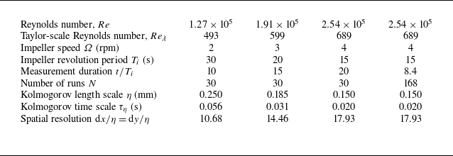
A summary of the experimental conditions for the decay measurements is provided in table 1. Velocity measurements were conducted for different initial impeller rotation rates 2, 3 and 4 rpm, corresponding to Reynolds numbers $Re=R^2\Omega /\nu =1.27\times 10^5$
,
$Re=R^2\Omega /\nu =1.27\times 10^5$
, $1.91\times 10^5$
and
$1.91\times 10^5$
and $2.54\times 10^5$
, respectively, where
$2.54\times 10^5$
, respectively, where $R$
is the impeller radius,
$R$
is the impeller radius, $\Omega$
is the angular velocity, and
$\Omega$
is the angular velocity, and $\nu =1.11\times 10^{-6}\ \textrm{m}^2\, \textrm{s}^{-1}$
is the kinematic viscosity of water at
$\nu =1.11\times 10^{-6}\ \textrm{m}^2\, \textrm{s}^{-1}$
is the kinematic viscosity of water at $16\ ^{\circ }\textrm{C}$
. The change in water temperature during the measurements was less than
$16\ ^{\circ }\textrm{C}$
. The change in water temperature during the measurements was less than $0.1\ ^{\circ }\textrm{C}$
. Each measurement was repeated a minimum of 30 times. The average measurement time was
$0.1\ ^{\circ }\textrm{C}$
. Each measurement was repeated a minimum of 30 times. The average measurement time was $t=300$
s, corresponding to 10, 15 and 20 impeller revolutions at 2, 3 and 4 rpm, respectively, with 400 velocity fields acquired per run. To test for convergence, 168 additional decay experiments were performed at 4 rpm, acquiring 180 velocity fields over a shorter duration
$t=300$
s, corresponding to 10, 15 and 20 impeller revolutions at 2, 3 and 4 rpm, respectively, with 400 velocity fields acquired per run. To test for convergence, 168 additional decay experiments were performed at 4 rpm, acquiring 180 velocity fields over a shorter duration $t=126$
s (8.4 revolutions). The comparison confirmed excellent consistency across all 258 tests. Steady-state flows at 2, 3 and 4 rpm were also measured to characterise the initial conditions of the turbulence, with 3000 velocity fields acquired for each case at 1.5 Hz.
$t=126$
s (8.4 revolutions). The comparison confirmed excellent consistency across all 258 tests. Steady-state flows at 2, 3 and 4 rpm were also measured to characterise the initial conditions of the turbulence, with 3000 velocity fields acquired for each case at 1.5 Hz.
Experimental conditions.
2.2. Measurement technique
A schematic of the stereoscopic PIV set-up is shown in figure 1(b). The coordinate system $(x, y, z)$
corresponds to the radial, axial and circumferential directions, with velocity components
$(x, y, z)$
corresponds to the radial, axial and circumferential directions, with velocity components $(U, V, W)$
. Two 16-bit LaVision Imager sCMOS cameras (2560
$(U, V, W)$
. Two 16-bit LaVision Imager sCMOS cameras (2560 $\times$
2160 pixels, with physical pixel size
$\times$
2160 pixels, with physical pixel size $6.5\,\unicode{x03BC} \textrm{m} \times 6.5\,\unicode{x03BC} \textrm{m}$
) fitted with Zeiss Milvus 2/100M lenses and Scheimpflug adapters were positioned
$6.5\,\unicode{x03BC} \textrm{m} \times 6.5\,\unicode{x03BC} \textrm{m}$
) fitted with Zeiss Milvus 2/100M lenses and Scheimpflug adapters were positioned $60^\circ$
apart on the same side of the laser sheet in a backward–forward scattering configuration. A dual-cavity pulsed ND:YAG laser (Litron Nano L 200-15 PIV, 200 mJ per pulse) served as the light source. Spherical particles (80
$60^\circ$
apart on the same side of the laser sheet in a backward–forward scattering configuration. A dual-cavity pulsed ND:YAG laser (Litron Nano L 200-15 PIV, 200 mJ per pulse) served as the light source. Spherical particles (80 $\unicode{x03BC}$
m diameter, 1.05 kg m–
$\unicode{x03BC}$
m diameter, 1.05 kg m– $^3$
density) were used for seeding, with average size
$^3$
density) were used for seeding, with average size $3 \times 3$
pixels in the images to minimise pixel locking. To measure the decaying flow, the time delay
$3 \times 3$
pixels in the images to minimise pixel locking. To measure the decaying flow, the time delay ${\rm d}t$
between camera frames and laser pulses was systematically increased to achieve particle displacement of approximately
${\rm d}t$
between camera frames and laser pulses was systematically increased to achieve particle displacement of approximately $1/4$
of the interrogation window in each snapshot. This was done by cumulative increases of
$1/4$
of the interrogation window in each snapshot. This was done by cumulative increases of $0.15$
ms to the starting
$0.15$
ms to the starting ${\rm d}t$
of 5, 3.5 and
${\rm d}t$
of 5, 3.5 and $2$
ms for 2, 3 and
$2$
ms for 2, 3 and $4$
rpm until
$4$
rpm until $400$
vector fields were recorded. A similar approach was used by Esteban et al. (Reference Esteban, Shrimpton and Ganapathisubramani2019). It is worth noting that the maximum
$400$
vector fields were recorded. A similar approach was used by Esteban et al. (Reference Esteban, Shrimpton and Ganapathisubramani2019). It is worth noting that the maximum ${\rm d}t$
possible for the experimental set-up was limited by the interframe transfer time of the cameras. The data were processed using LaVision Davis 10, using multi-pass cross-correlation with final interrogation window size
${\rm d}t$
possible for the experimental set-up was limited by the interframe transfer time of the cameras. The data were processed using LaVision Davis 10, using multi-pass cross-correlation with final interrogation window size $32\times 32$
and
$32\times 32$
and $75\, \%$
window overlap and self-calibration. This gave a spatial resolution, based on the interrogation window size,
$75\, \%$
window overlap and self-calibration. This gave a spatial resolution, based on the interrogation window size, $2.67\:\textrm{mm}\times 2.67\:\textrm{mm}$
corresponding to normalised resolution 10
$2.67\:\textrm{mm}\times 2.67\:\textrm{mm}$
corresponding to normalised resolution 10 $\eta$
–18
$\eta$
–18 $\eta$
as shown in table 1. The effective magnification of the cameras was 0.083 mm pixel–1. Estimating the spatial resolution following the approach of Foucaut et al. (Reference Foucaut, Carlier and Stanislas2004) based on a
$\eta$
as shown in table 1. The effective magnification of the cameras was 0.083 mm pixel–1. Estimating the spatial resolution following the approach of Foucaut et al. (Reference Foucaut, Carlier and Stanislas2004) based on a $3\ \textrm{dB}$
attenuation of the spectral response due to the applied windowing was
$3\ \textrm{dB}$
attenuation of the spectral response due to the applied windowing was $5.99$
mm.
$5.99$
mm.
3. Results
3.1. Stationary turbulence
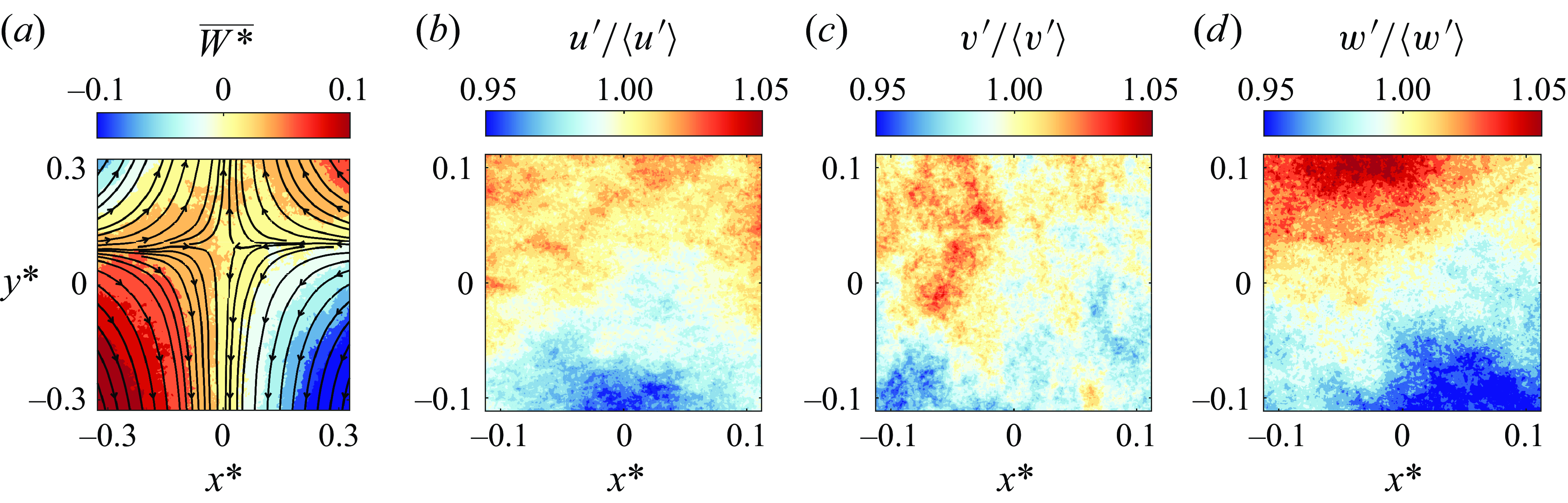
Steady-state conditions were first established before abruptly stopping the impellers to measure the turbulent decay rates. These form the initial conditions of the decay experiments and are therefore described briefly. The normalised mean flow and velocity fluctuations of the highest Reynolds number case (4 rpm) are shown in figure 2, with associated turbulent statistics in table 2. As the measurements were insufficiently resolved for direct calculation of the small scales, the fits $Re_{\lambda }=1.75\,Re^{0.482}$
and
$Re_{\lambda }=1.75\,Re^{0.482}$
and $\eta /R = 1.98\, Re^{-0.748}$
from volumetric measurements provided in Worth (Reference Worth2010) were used. These fits have been well characterised in later experiments via spherical correlations from the volumetric measurements of Lawson & Dawson (Reference Lawson and Dawson2014, Reference Lawson and Dawson2015) in the same apparatus.
$\eta /R = 1.98\, Re^{-0.748}$
from volumetric measurements provided in Worth (Reference Worth2010) were used. These fits have been well characterised in later experiments via spherical correlations from the volumetric measurements of Lawson & Dawson (Reference Lawson and Dawson2014, Reference Lawson and Dawson2015) in the same apparatus.
Turbulence statistics of the stationary flow (initial conditions).
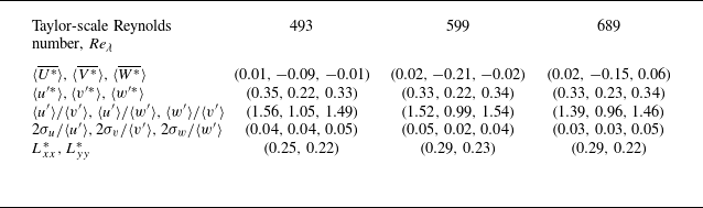
We denote ensemble averages over repeated measurements at the same normalised time step with an overline, spatial averages over the PIV field of view with angle brackets ( $\langle \cdot \rangle$
) and normalised quantities with an asterisk (
$\langle \cdot \rangle$
) and normalised quantities with an asterisk ( $ ^\ast$
), where units of length are normalised by the impeller radius
$ ^\ast$
), where units of length are normalised by the impeller radius $R$
, and velocities are normalised by the impeller tip velocity
$R$
, and velocities are normalised by the impeller tip velocity $R\Omega$
. The prime symbol (
$R\Omega$
. The prime symbol ( $^\prime$
) is used to denote the root mean square (r.m.s.) of the component velocity fluctuations such that
$^\prime$
) is used to denote the root mean square (r.m.s.) of the component velocity fluctuations such that $u_i^\prime = (\overline {u_i^2})^{1/2}$
.
$u_i^\prime = (\overline {u_i^2})^{1/2}$
.
Figure 2(a) presents a larger field of view than used in the decay experiments to highlight the mean flow pattern. The streamlines show the inward radial flow and outward axial flow from the centre of the tank resembling a stagnation flow where the mean velocity is negligible and the flow is dominated by turbulent fluctuations that were previously shown to be homogeneous via resolved volumetric measurements (Lawson & Dawson Reference Lawson and Dawson2014, Reference Lawson and Dawson2015). The colour-filled contours correspond to the mean out-of-plane velocity component in the circumferential direction of the tank, $\overline {W^*}$
, which captures part of the large-scale toroidal and poloidal flow motions. The values of the mean component velocities and fluctuations are shown in table 2. Figures 2(b), 2(c) and 2(d) plot fields of the normalised velocity fluctuations r.m.s. in the radial, axial and circumferential directions, respectively. The normalised r.m.s. fluctuations are close to 1, which indicates that the turbulence is reasonably homogeneous. Further confirmation of the homogeneity for each
$\overline {W^*}$
, which captures part of the large-scale toroidal and poloidal flow motions. The values of the mean component velocities and fluctuations are shown in table 2. Figures 2(b), 2(c) and 2(d) plot fields of the normalised velocity fluctuations r.m.s. in the radial, axial and circumferential directions, respectively. The normalised r.m.s. fluctuations are close to 1, which indicates that the turbulence is reasonably homogeneous. Further confirmation of the homogeneity for each $Re_{\lambda }$
in the decay experiments is evaluated using the ratio
$Re_{\lambda }$
in the decay experiments is evaluated using the ratio $2\sigma _{u_i}/\langle u'_i \rangle$
, where the pre-factor ensures a 95 % confidence interval (Esteban et al. Reference Esteban, Shrimpton and Ganapathisubramani2019), as well as the level of isotropy, evaluated via r.m.s. ratios, shown in table 2. These show that the radial and circumferential components are nearly isotropic,
$2\sigma _{u_i}/\langle u'_i \rangle$
, where the pre-factor ensures a 95 % confidence interval (Esteban et al. Reference Esteban, Shrimpton and Ganapathisubramani2019), as well as the level of isotropy, evaluated via r.m.s. ratios, shown in table 2. These show that the radial and circumferential components are nearly isotropic, $\langle u' \rangle /\langle w' \rangle =0.96$
, but deviations appear when axial components
$\langle u' \rangle /\langle w' \rangle =0.96$
, but deviations appear when axial components $\langle v' \rangle$
are included. The longitudinal integral length scales of the flow (
$\langle v' \rangle$
are included. The longitudinal integral length scales of the flow ( $L_{ii}^*$
) in the
$L_{ii}^*$
) in the $x$
and
$x$
and $y$
directions at the start of the decay experiments were calculated from the PIV data by evaluating the area under the curve of the normalised autocorrelation functions as described in Pope (Reference Pope2000).
$y$
directions at the start of the decay experiments were calculated from the PIV data by evaluating the area under the curve of the normalised autocorrelation functions as described in Pope (Reference Pope2000).
(a) Normalised mean velocities of the stationary flow, where $\overline {U^*}$
and
$\overline {U^*}$
and $\overline {V^*}$
vectors are shown as the streamlines, while
$\overline {V^*}$
vectors are shown as the streamlines, while $\overline {W^*}$
is shown as colour-filled contours. (b–d) Normalised ensemble-averaged contours of the r.m.s. of the component velocity fluctuations
$\overline {W^*}$
is shown as colour-filled contours. (b–d) Normalised ensemble-averaged contours of the r.m.s. of the component velocity fluctuations $u'_i/\langle u'_i\rangle$
.
$u'_i/\langle u'_i\rangle$
.
Temporal decay of (a) the TKE $k^*(t^*)$
and (b) the contribution from different velocity components
$k^*(t^*)$
and (b) the contribution from different velocity components $k_i^*(t^*)$
.
$k_i^*(t^*)$
.
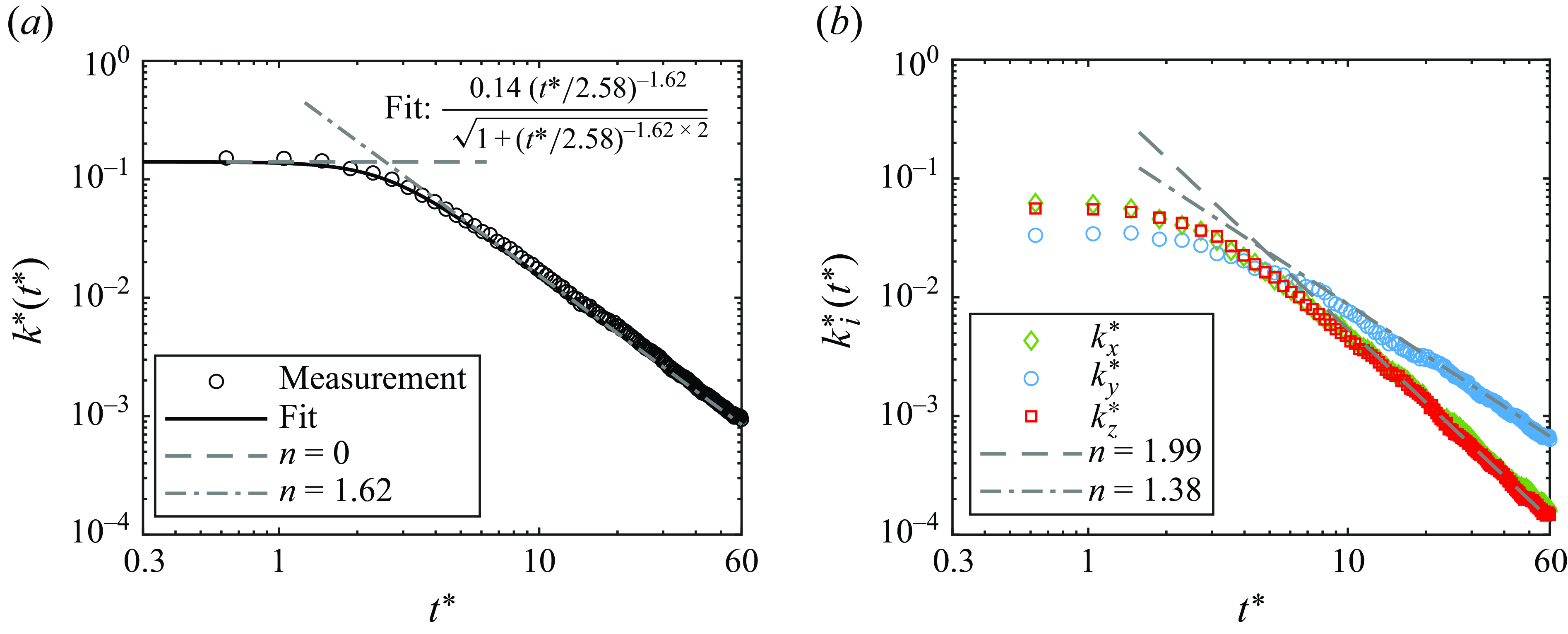
3.2. Decaying turbulence
In this subsection, we present the results of the temporal decay measurements after abruptly stopping the impellers. For each Reynolds number shown in table 1, we first calculate an ensemble-averaged velocity field $\overline {U_i^*}(\boldsymbol{x}^*,t^*)$
over each of the 30 runs for each non-dimensional time step during the decay. We then perform a Reynolds decomposition to obtain component fluctuation fields for
$\overline {U_i^*}(\boldsymbol{x}^*,t^*)$
over each of the 30 runs for each non-dimensional time step during the decay. We then perform a Reynolds decomposition to obtain component fluctuation fields for $u^*, v^*, w^*$
at each non-dimensional time step. Finally, we calculate the TKE by ensemble averaging the component fluctuation square fields, and then spatial averaging them to get a single value at each time step using the expression
$u^*, v^*, w^*$
at each non-dimensional time step. Finally, we calculate the TKE by ensemble averaging the component fluctuation square fields, and then spatial averaging them to get a single value at each time step using the expression $k^*(t^*)=0.5\langle \overline {u^{*2}+v^{*2}+w^{*2}}\rangle$
. Similarly, we evaluated the decay in TKE for each of the velocity components
$k^*(t^*)=0.5\langle \overline {u^{*2}+v^{*2}+w^{*2}}\rangle$
. Similarly, we evaluated the decay in TKE for each of the velocity components $k^*_x(t^*)=0.5\langle \overline {u^{*2}}\rangle$
,
$k^*_x(t^*)=0.5\langle \overline {u^{*2}}\rangle$
, $k^*_y(t^*)=0.5\langle \overline {v^{*2}}\rangle$
and
$k^*_y(t^*)=0.5\langle \overline {v^{*2}}\rangle$
and $k^*_z(t^*)=0.5\langle \overline {w^{*2}}\rangle$
, where
$k^*_z(t^*)=0.5\langle \overline {w^{*2}}\rangle$
, where $k^*(t^*) = k^*_x(t^*) + k^*_y(t^*) + k^*_z(t^*)$
. When plotting the decay curves for each Reynolds number, it was found that they collapsed when plotted using normalised values of
$k^*(t^*) = k^*_x(t^*) + k^*_y(t^*) + k^*_z(t^*)$
. When plotting the decay curves for each Reynolds number, it was found that they collapsed when plotted using normalised values of $k^*$
and
$k^*$
and $t^*$
. In other words, the decay of TKE was found to be independent of the Reynolds numbers tested. We therefore plot the temporal evolution of the total and component TKE averaged over all cases in figure 3 on a log-log scale.
$t^*$
. In other words, the decay of TKE was found to be independent of the Reynolds numbers tested. We therefore plot the temporal evolution of the total and component TKE averaged over all cases in figure 3 on a log-log scale.
Figure 3(a) shows that the total $k^*(t^*)$
follows a clear and smooth pattern of decay covering more than two decades after the impellers are stopped. The decay process is preceded by an initial phase where
$k^*(t^*)$
follows a clear and smooth pattern of decay covering more than two decades after the impellers are stopped. The decay process is preceded by an initial phase where $k^*$
is approximately constant followed by a short transition before reaching a negative exponent power-law decay rate. As the figure is very similar to the form of a one-dimensional energy spectrum, it was found that we could represent this behaviour by a single fit by adopting a similar approach to modelling the one-dimensional energy spectrum at small wavenumbers as described in Pope (Reference Pope2000) using the equation
$k^*$
is approximately constant followed by a short transition before reaching a negative exponent power-law decay rate. As the figure is very similar to the form of a one-dimensional energy spectrum, it was found that we could represent this behaviour by a single fit by adopting a similar approach to modelling the one-dimensional energy spectrum at small wavenumbers as described in Pope (Reference Pope2000) using the equation
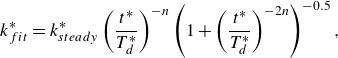 \begin{equation} k^*_{{fit}} = k^*_{{steady}} \left (\frac {t^*}{T^*_{{d}}}\right )^{-n}\left (1+\left (\frac {t^*}{T^*_{{d}}}\right )^{-2n}\right )^{-0.5}, \end{equation}
where the fit coefficients $k^*_{{steady}}$
,
$k^*_{{steady}}$
, $n$
and
$n$
and $T^*_{{d}}$
represent the steady-state energy, power-law decay exponent and initial transition time, respectively. This ansatz eliminates the ambiguity of the virtual origin position (Panickacheril John et al. Reference Panickacheril John, Donzis and Sreenivasan2022), enabling consistent estimation of the decay exponent
$T^*_{{d}}$
represent the steady-state energy, power-law decay exponent and initial transition time, respectively. This ansatz eliminates the ambiguity of the virtual origin position (Panickacheril John et al. Reference Panickacheril John, Donzis and Sreenivasan2022), enabling consistent estimation of the decay exponent $n$
. For small
$n$
. For small $t^*$
, the function simplifies to
$t^*$
, the function simplifies to $k^*_{fit} = k^*_{{steady}}$
, whilst for large
$k^*_{fit} = k^*_{{steady}}$
, whilst for large $t^*$
, it follows a classical power-law decay:
$t^*$
, it follows a classical power-law decay: $k^*_{fit} = k^*_{{steady}}(t^*/T^*_{{d}})^{-n}$
. Fitting this function to the measured data shown by the solid line in figure 3(a) yields decay exponent
$k^*_{fit} = k^*_{{steady}}(t^*/T^*_{{d}})^{-n}$
. Fitting this function to the measured data shown by the solid line in figure 3(a) yields decay exponent $n=1.62$
and transition time
$n=1.62$
and transition time $T^*_{\textrm{d}}=2.58$
, which corresponds to
$T^*_{\textrm{d}}=2.58$
, which corresponds to $2.58/2\unicode{x03C0} =0.41$
impeller rotations. The decay exponent
$2.58/2\unicode{x03C0} =0.41$
impeller rotations. The decay exponent $n=1.62$
indicates a faster decay than the theoretical predictions by Birkhoff and Saffman (
$n=1.62$
indicates a faster decay than the theoretical predictions by Birkhoff and Saffman ( $n=6/5=1.2$
) and Loitsiansky (
$n=6/5=1.2$
) and Loitsiansky ( $n=10/7\approx 1.43$
), but it lies within the range of self-similarity (
$n=10/7\approx 1.43$
), but it lies within the range of self-similarity ( $n=1$
) and scaling arguments (
$n=1$
) and scaling arguments ( $n=2$
).
$n=2$
).
By decomposing the decay of TKE into contributions from individual velocity components, we can assess whether the decay rate is isotropic or anisotropic. Figure 3(b) shows the temporal decay of radial, axial and circumferential components. The axial component ( $k^*_y$
) decays more slowly than the radial (
$k^*_y$
) decays more slowly than the radial ( $k^*_x$
) and circumferential (
$k^*_x$
) and circumferential ( $k^*_z$
) components, which have similar decay rates. The corresponding decay exponents were found to be
$k^*_z$
) components, which have similar decay rates. The corresponding decay exponents were found to be $n_y=1.38$
and
$n_y=1.38$
and $n_x=n_z=1.99$
. The value
$n_x=n_z=1.99$
. The value $n_y=1.38$
is in good agreement with Loitsiansky’s prediction and values reported in grid turbulence studies (Comte-Bellot & Corrsin Reference Comte-Bellot and Corrsin1966; Van Atta & Chen Reference Van Atta and Chen1969; Sirivat & Warhaft Reference Sirivat and Warhaft1983; Mohamed & Larue Reference Mohamed and Larue1990; Hearst & Lavoie Reference Hearst and Lavoie2014), stationary turbulence (Esteban et al. Reference Esteban, Shrimpton and Ganapathisubramani2019), and numerical simulations (Ishida et al. Reference Ishida, Davidson and Kaneda2006; Thornber et al. Reference Thornber, Mosedale and Drikakis2007; Meldi et al. Reference Meldi, Sagaut and Lucor2011; Meldi & Sagaut Reference Meldi and Sagaut2017; Yu et al. Reference Yu, Colonius, Pullin and Winckelmans2021). In contrast,
$n_y=1.38$
is in good agreement with Loitsiansky’s prediction and values reported in grid turbulence studies (Comte-Bellot & Corrsin Reference Comte-Bellot and Corrsin1966; Van Atta & Chen Reference Van Atta and Chen1969; Sirivat & Warhaft Reference Sirivat and Warhaft1983; Mohamed & Larue Reference Mohamed and Larue1990; Hearst & Lavoie Reference Hearst and Lavoie2014), stationary turbulence (Esteban et al. Reference Esteban, Shrimpton and Ganapathisubramani2019), and numerical simulations (Ishida et al. Reference Ishida, Davidson and Kaneda2006; Thornber et al. Reference Thornber, Mosedale and Drikakis2007; Meldi et al. Reference Meldi, Sagaut and Lucor2011; Meldi & Sagaut Reference Meldi and Sagaut2017; Yu et al. Reference Yu, Colonius, Pullin and Winckelmans2021). In contrast, $n_x=n_z=1.99$
closely matches the saturation decay exponent (
$n_x=n_z=1.99$
closely matches the saturation decay exponent ( $n=2$
) predicted by Skrbek & Stalp (Reference Skrbek and Stalp2000) and observed in the experiment of Esteban et al. (Reference Esteban, Shrimpton and Ganapathisubramani2019), which was attributed to confinement effects. The decay exponents for different velocity components indicate a classical unsaturated decay regime in the axial direction, where the component flow is moving away in the normal direction relative to the shear layer produced by the large poloidal vortices, and a saturated decay regime in the radial and circumferential directions, where the component flow is moving parallel to the shear layer. It is worth further comment that the turbulent decay rate along the symmetry axis of rotation follows Loitsiansky’s prediction, which is based on the conservation of angular momentum. Although Loitsiansky assumed isotropy, our results in figure 3(b) suggest that rate of turbulent decay in von Kármán flows may feature a preferred direction (the axial direction) that is normal to the applied angular momentum of the impellers. A possible explanation for this is that the geometry may impose a directional preference that selectively conserves of angular momentum in specific component directions, leading to different decay exponents.
$n=2$
) predicted by Skrbek & Stalp (Reference Skrbek and Stalp2000) and observed in the experiment of Esteban et al. (Reference Esteban, Shrimpton and Ganapathisubramani2019), which was attributed to confinement effects. The decay exponents for different velocity components indicate a classical unsaturated decay regime in the axial direction, where the component flow is moving away in the normal direction relative to the shear layer produced by the large poloidal vortices, and a saturated decay regime in the radial and circumferential directions, where the component flow is moving parallel to the shear layer. It is worth further comment that the turbulent decay rate along the symmetry axis of rotation follows Loitsiansky’s prediction, which is based on the conservation of angular momentum. Although Loitsiansky assumed isotropy, our results in figure 3(b) suggest that rate of turbulent decay in von Kármán flows may feature a preferred direction (the axial direction) that is normal to the applied angular momentum of the impellers. A possible explanation for this is that the geometry may impose a directional preference that selectively conserves of angular momentum in specific component directions, leading to different decay exponents.
The evolutions of the longitudinal integral length scales in the radial ( $L^*_{xx}$
) and axial (
$L^*_{xx}$
) and axial ( $L^*_{yy}$
) directions are plotted in Figure 4(a). The autocorrelation function
$L^*_{yy}$
) directions are plotted in Figure 4(a). The autocorrelation function $\rho _{i}(\boldsymbol{r}^{*}, t^*)=\int _{{FoV}} u_i^{*}(\boldsymbol{x}^{*},t^*)\, u_i^{*}(\boldsymbol{x}^{*}+\boldsymbol{r}^{*},t^*)\,\textrm{d}\boldsymbol{x}^{*}{\Big/\int _{{FoV}} u_i^{*}(\boldsymbol{x}^{*},t^*)\, u_i^{*}(\boldsymbol{x}^{*},t^*)\,\textrm{d}\boldsymbol{x}^{*}}$
was calculated for each snapshot, where
$\rho _{i}(\boldsymbol{r}^{*}, t^*)=\int _{{FoV}} u_i^{*}(\boldsymbol{x}^{*},t^*)\, u_i^{*}(\boldsymbol{x}^{*}+\boldsymbol{r}^{*},t^*)\,\textrm{d}\boldsymbol{x}^{*}{\Big/\int _{{FoV}} u_i^{*}(\boldsymbol{x}^{*},t^*)\, u_i^{*}(\boldsymbol{x}^{*},t^*)\,\textrm{d}\boldsymbol{x}^{*}}$
was calculated for each snapshot, where $\boldsymbol{r}^{*}$
is the normalised separation vector. An exponential function of the form
$\boldsymbol{r}^{*}$
is the normalised separation vector. An exponential function of the form $\exp (-r^*/L_{ii}^*)$
was fitted to the ensemble-averaged autocorrelation function
$\exp (-r^*/L_{ii}^*)$
was fitted to the ensemble-averaged autocorrelation function $\overline {\rho _i}$
along the
$\overline {\rho _i}$
along the $i$
direction of the separation vector to estimate
$i$
direction of the separation vector to estimate $L_{ii}^*$
(Reynolds & Castro Reference Reynolds and Castro2008). During the initial phase, the length scales are preserved, after which the growth in the axial direction follows a power law with exponent
$L_{ii}^*$
(Reynolds & Castro Reference Reynolds and Castro2008). During the initial phase, the length scales are preserved, after which the growth in the axial direction follows a power law with exponent $m_y \approx 2/7 = 0.29$
, which is also consistent with Loitsiansky’s prediction
$m_y \approx 2/7 = 0.29$
, which is also consistent with Loitsiansky’s prediction $m = 2/7 = 0.286$
. This is in contrast to the radial integral length scale, which remains nearly constant,
$m = 2/7 = 0.286$
. This is in contrast to the radial integral length scale, which remains nearly constant, $m_x \approx 0$
. Both the decay rates and growth of integral length scales demonstrate classical behaviour in axial components, while the radial direction exhibits a saturation or confinement effect.
$m_x \approx 0$
. Both the decay rates and growth of integral length scales demonstrate classical behaviour in axial components, while the radial direction exhibits a saturation or confinement effect.
(a) Temporal evolution of longitudinal integral length scales $L^*_{xx}$
and
$L^*_{xx}$
and $L^*_{yy}$
from the PIV data. (b) Temporal decay of the mean velocity gradients.
$L^*_{yy}$
from the PIV data. (b) Temporal decay of the mean velocity gradients.
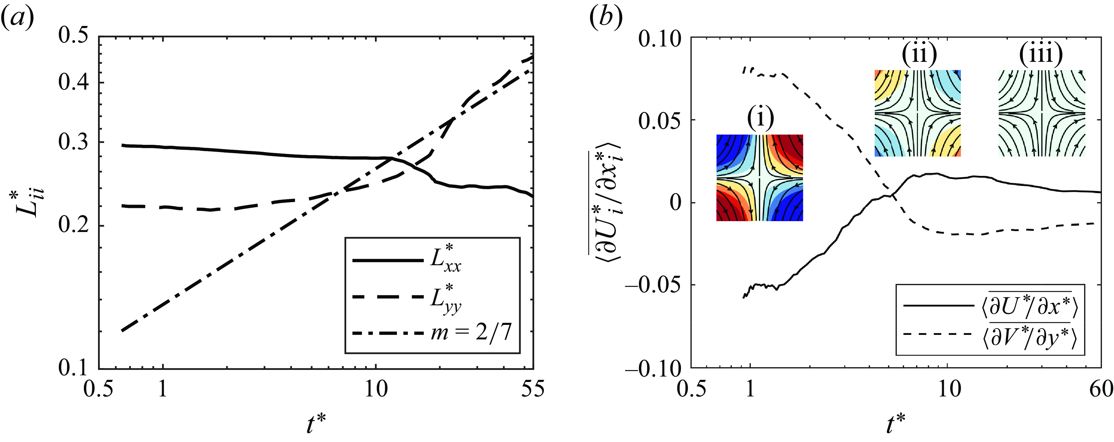
Finally, we examine the evolution of the mean velocity gradients. Near the stagnation point, the stationary mean flow can be approximated by uniform velocity gradients: $ \overline {U_i^*}(x^*,y^*) = \langle \overline {\partial U_i^*/\partial x^*}\rangle (x^*-x_0^*) + \langle \overline {\partial U_i^*/\partial y^*}\rangle (y^*-y_0^*)$
, where
$ \overline {U_i^*}(x^*,y^*) = \langle \overline {\partial U_i^*/\partial x^*}\rangle (x^*-x_0^*) + \langle \overline {\partial U_i^*/\partial y^*}\rangle (y^*-y_0^*)$
, where $(x_0^*,y_0^*)$
is the stagnation point (Lawson & Dawson Reference Lawson and Dawson2015; Knutsen et al. Reference Knutsen, Baj, Lawson, Bodenschatz, Dawson and Worth2020). In figure 4(b), we plot the normalised decay of the ensemble-averaged velocity gradients
$(x_0^*,y_0^*)$
is the stagnation point (Lawson & Dawson Reference Lawson and Dawson2015; Knutsen et al. Reference Knutsen, Baj, Lawson, Bodenschatz, Dawson and Worth2020). In figure 4(b), we plot the normalised decay of the ensemble-averaged velocity gradients $\langle \overline {\partial U^* /\partial x^*}\rangle (t^*)$
and
$\langle \overline {\partial U^* /\partial x^*}\rangle (t^*)$
and $\langle \overline {\partial V^* /\partial y^*}\rangle (t^*)$
. During the initial phase (early
$\langle \overline {\partial V^* /\partial y^*}\rangle (t^*)$
. During the initial phase (early $t^*$
), the gradient signs match the stationary flow pattern under steady flow conditions (inset i) and their magnitudes decrease until
$t^*$
), the gradient signs match the stationary flow pattern under steady flow conditions (inset i) and their magnitudes decrease until $t^* \approx 4$
, after which the gradients then reverse sign (inset ii) implying a large-scale flow inversion. The gradients then reach a local maximum and decay towards zero (inset iii). These results show that after the impellers are stopped, the stationary mean flow persists due to inertia, undergoes a flow reversal, and then decays. Comparing the timing of these transitions with the decay rates in figure 3 strongly suggests that the power-law decay begins only after the large-scale flow reversal. The underlying mechanisms of this reversal currently remain unclear. However, it is conjectured that the flow reversal is likely triggered by the interaction between the inertia of the upper and lower toroidal flows when the impellers are suddenly stopped, and the viscous drag imparted by the stationary impellers to ensure conservation of angular momentum.
$t^* \approx 4$
, after which the gradients then reverse sign (inset ii) implying a large-scale flow inversion. The gradients then reach a local maximum and decay towards zero (inset iii). These results show that after the impellers are stopped, the stationary mean flow persists due to inertia, undergoes a flow reversal, and then decays. Comparing the timing of these transitions with the decay rates in figure 3 strongly suggests that the power-law decay begins only after the large-scale flow reversal. The underlying mechanisms of this reversal currently remain unclear. However, it is conjectured that the flow reversal is likely triggered by the interaction between the inertia of the upper and lower toroidal flows when the impellers are suddenly stopped, and the viscous drag imparted by the stationary impellers to ensure conservation of angular momentum.
4. Conclusion
In this paper, the decay of stationary turbulence at Reynolds numbers based on the Taylor microscale $Re_{\lambda }=493, 599, 689$
produced in a von Kármán flow was investigated using stereoscopic PIV. To characterise the initial conditions of the decay experiments, measurements were obtained to characterise the turbulence under steady flow conditions (constant impeller rotation speeds). To initiate the decay experiments, the impellers were stopped and the turbulent decay was measured over 10–20 impeller rotation periods. A total of 258 decay experiments were performed. To the best of the authors’ knowledge, this is the first reporting of turbulent decay measured in a von Kármán flow.
$Re_{\lambda }=493, 599, 689$
produced in a von Kármán flow was investigated using stereoscopic PIV. To characterise the initial conditions of the decay experiments, measurements were obtained to characterise the turbulence under steady flow conditions (constant impeller rotation speeds). To initiate the decay experiments, the impellers were stopped and the turbulent decay was measured over 10–20 impeller rotation periods. A total of 258 decay experiments were performed. To the best of the authors’ knowledge, this is the first reporting of turbulent decay measured in a von Kármán flow.
The decay in TKE showed excellent agreement over all $Re_{\lambda }$
and exhibited two distinct phases. After stopping the impellers, the inertia of the flow resulting in an initial plateau where the TKE was constant and lasted
$Re_{\lambda }$
and exhibited two distinct phases. After stopping the impellers, the inertia of the flow resulting in an initial plateau where the TKE was constant and lasted $\approx 0.4$
impeller rotations, followed by a transition to a power-law decay. A fitting function, based on a one-dimensional energy spectrum, was used and successfully captured the entire measured decay process, eliminating any ambiguities encountered when defining the virtual start point. A power-law decay exponent
$\approx 0.4$
impeller rotations, followed by a transition to a power-law decay. A fitting function, based on a one-dimensional energy spectrum, was used and successfully captured the entire measured decay process, eliminating any ambiguities encountered when defining the virtual start point. A power-law decay exponent $n=1.62$
was obtained for the ensemble average at all
$n=1.62$
was obtained for the ensemble average at all $Re_{\lambda }$
. However, different decay exponents were found when considering the velocity components. The decay exponent of the axial velocity component, which is normal to the applied angular momentum of the impellers, was
$Re_{\lambda }$
. However, different decay exponents were found when considering the velocity components. The decay exponent of the axial velocity component, which is normal to the applied angular momentum of the impellers, was $n_y=1.38$
, consistent with various reports in the literature and Loitsiansky’s theoretical prediction
$n_y=1.38$
, consistent with various reports in the literature and Loitsiansky’s theoretical prediction $n=1.43$
, which is based on the conservation of angular momentum. The radial and circumferential components yielded
$n=1.43$
, which is based on the conservation of angular momentum. The radial and circumferential components yielded $n_x=n_z=1.99$
, indicative of saturation/confinement effects. This raises the possibility that the geometry of von Kármán flows may impose a directional preference in the turbulent decay rate that selectively conserves angular momentum in specific component directions, leading to different decay exponents. Similar behaviour in the growth of the longitudinal integral length scales was also observed as
$n_x=n_z=1.99$
, indicative of saturation/confinement effects. This raises the possibility that the geometry of von Kármán flows may impose a directional preference in the turbulent decay rate that selectively conserves angular momentum in specific component directions, leading to different decay exponents. Similar behaviour in the growth of the longitudinal integral length scales was also observed as $L^*_{yy} \propto t^{*2/7}$
(
$L^*_{yy} \propto t^{*2/7}$
( $m_y=2/7$
), whilst
$m_y=2/7$
), whilst $L^*_{xx}$
remained nearly constant.
$L^*_{xx}$
remained nearly constant.
Finally, the evolution of the ensemble-averaged velocity gradients showed that after the impellers were stopped, the mean flow pattern persisted for a short time before undergoing a large-scale reversal before the turbulent decay. Although the mechanisms behind this large-scale flow reversal remain unclear, we conjecture that it is likely triggered by the interaction between the inertia of the upper and lower toroidal flows and the viscous drag imparted by the stationary impellers to conserve angular momentum. Further studies are needed to identify whether such large scale reorganisations observed herein are a general feature of not only von Kármán flows but also other rotating flows such as toroidal flows or Ekman flow.
Funding.
P.B. acknowledges financial support for the research leading to these results received from the Norwegian Financial Mechanism 2014–2021 (project no. 2020/37/K/ST8/02594).
Declaration of interests.
The authors report no conflict of interest.


 Open access