


1. Introduction
Plasma simulations have historically utilized supercomputers to accurately predict and understand the behaviour of electromagnetic plasmas in large-scale astrophysical phenomena, nuclear fusion energy systems and the engineering evaluation of space industry and semiconductor products. Numerical simulation methods for predicting plasma motion are generally categorized according to the spatial and temporal scales. For instance, simulations at microscopic scales utilize particle-in-cell (PIC) simulations and Vlasov–Maxwell (or Vlasov–Poisson) simulations, while at macroscopic scales, magnetohydrodynamic (MHD) simulations, which involve static relaxation and fluid approximations, are employed. As computing technology has advanced, PIC-MHD and Vlasov-MHD simulations that connect these hierarchical scales, as well as low-resolution full-PIC and full-Vlasov simulations, have been developed. This has led to a better understanding of multiscale plasma phenomena, such as magnetic reconnection. However, none have achieved significant increases in simulation size due to the immense computational costs involved. It is an important task to seek methods that can consistently simulate all multiscale plasma physical phenomena. This necessitates the development of computational methods capable of simultaneously handling microscopic kinetic effects and macroscopic MHD turbulence.
We focus on the Vlasov–Maxwell equations in plasma simulations. The primary challenge of Vlasov simulations is the high computational cost required for the time evolution of the six-dimensional partial differential equations (PDEs). Assuming that the Vlasov equation can be divided into six advection equations and that each advection equation is solved using a simple explicit method, the computational complexity of classical calculations becomes $O(N^6(T^2/\epsilon +cT/\Delta x))$
from Remark 1 in (Sato et al. Reference Sato, Kondo, Hamamura, Onodera and Yamamoto2024). Here,
$O(N^6(T^2/\epsilon +cT/\Delta x))$
from Remark 1 in (Sato et al. Reference Sato, Kondo, Hamamura, Onodera and Yamamoto2024). Here, $N$
is the number of isotropic and uniform grids for each six-dimensional direction,
$N$
is the number of isotropic and uniform grids for each six-dimensional direction, $T$
is the simulation time,
$T$
is the simulation time, $\epsilon$
is the error tolerance,
$\epsilon$
is the error tolerance, $c$
is the advection velocity and
$c$
is the advection velocity and $\Delta x$
is the spatial grid width.
$\Delta x$
is the spatial grid width.
In recent years, the development of quantum algorithms for classical PDEs assuming fault-tolerant quantum computers has rapidly progressed. Notable examples include algorithms for the Navier–Stokes equations (Gaitan Reference Gaitan2020,Reference Gaitan2021), the Vlasov equation (Engel, Smith & Parker Reference Engel, Smith and Parker2019; Ameri et al. Reference Ameri, Ye, Cappellaro, Krovi and Loureiro2023; Miyamoto et al. Reference Miyamoto, Yamazaki, Uchida, Fujisawa and Yoshida2024; Toyoizumi, Yamamoto & Hoshino Reference Toyoizumi, Yamamoto and Hoshino2024), the Poisson equation (Cao et al. Reference Cao, Papageorgiou, Petras, Traub and Kais2013; Wang et al. Reference Wang, Wang, Li, Fan, Wei and Gu2020) and the wave equation (Costa, Jordan & Ostrander Reference Costa, Jordan and Ostrander2019; Suau, Staffelbach & Calandra Reference Suau, Staffelbach and Calandra2021). Quantum algorithms for linear ordinary differential equations, such as the HHL algorithm (Harrow, Hassidim & Lloyd Reference Harrow, Hassidim and Lloyd2009; Childs, Kothari & Somma Reference Childs, Kothari and Somma2017) and Hamiltonian simulation algorithms (Berry et al. Reference Berry, Ahokas, Cleve and Sanders2007; Childs & Kothari Reference Childs and Kothari2010; Berry & Childs Reference Berry and Childs2012; Childs & Wiebe Reference Childs and Wiebe2012; Berry et al. Reference Berry, Childs, Cleve, Kothari and Somma2014, Reference Berry, Childs, Cleve, Kothari and Somma2015a ,Reference Berry, Childs and Kothari b ; Berry & Novo Reference Berry and Novo2016; Novo & Berry Reference Novo and Berry2017; Childs et al. Reference Childs, Maslov, Nam, Ross and Su2018), have been proposed to potentially provide exponential speedup. Efficient implementation of the Hamiltonian simulation has mainly utilized the Trotter decomposition algorithm (Jin, Liu & Yu Reference Jin, Liu and Yu2023; Jin et al. Reference Jin, Liu and Ma2024), or quantum singular value transformation (QSVT) algorithm (Gilyén et al. Reference Gilyén, Su, Low and Wiebe2019). Sato et al. (Reference Sato, Kondo, Hamamura, Onodera and Yamamoto2024) demonstrated quantum computation of advection and wave equations using Hamiltonian simulation with Trotter decomposition, highlighting issues with spatial discretization using central difference and errors unique to Trotter decomposition from a numerical computation scheme perspective. Hu et al. (Reference Hu, Jin, Liu and Zhang2024) illustrated a method for ‘Schrödingerization’ of spatial discretization using upwind differences under specific conditions. There is a growing trend towards enhancing the accuracy of quantum computational methods in line with the history of classical numerical computation.
Various plasma physics problems have been explored for potential applications to quantum computing (Dodin & Startsev Reference Dodin and Startsev2021). Plasma simulations are typically formulated as coupled sets of nonlinear PDEs, and thus transforming them into linear Schrödinger equations is not straightforward. However, wave problems, such as three-wave interactions in plasma (Shi et al. Reference Shi2021) and extraordinary waves in cold plasma (electromagnetic waves with electric fields perpendicular to the background magnetic field) (Novikau, Startsev & Dodin Reference Novikau, Startsev and Dodin2022), have been efficiently mapped to Schrödinger equations. Ideally, a quantum algorithm capable of solving the first-principles description of plasma physics provided by the Vlasov equation is desired. For problems with weak nonlinearity, implementation methods for linearizing and performing Hamiltonian simulation on the Vlasov–Maxwell equations (Engel et al. Reference Engel, Smith and Parker2019), the collisional Vlasov–Poisson equations (Ameri et al. Reference Ameri, Ye, Cappellaro, Krovi and Loureiro2023) and the Vlasov–Poisson equations (Toyoizumi et al. Reference Toyoizumi, Yamamoto and Hoshino2024) have been demonstrated within the framework of spectral methods under static assumptions. Specifically, Toyoizumi et al. (Reference Toyoizumi, Yamamoto and Hoshino2024) employ the Hamiltonian simulation based on QSVT, allowing the application to different problems by merely changing the block-encoding quantum circuits of the Hamiltonian.
However, linearizing the nonlinear Vlasov–Maxwell equations using quantum algorithms for nonlinear differential equations is challenging. For example, both Carleman linearization (Carleman Reference Carleman1932; Kowalski & Steeb Reference Kowalski and Steeb1991; Liu et al. Reference Liu, Kolden, Krovi, Loureiro, Trivisa and Childs2021) and Koopman–von Neumann linearization (Koopman Reference Koopman1931; Neumann Reference Neumann1932) are hindered by the first moment calculation term of the current density within the system of equations. Consequently, among the existing quantum algorithms, solving the genuinely nonlinear Vlasov–Maxwell equations requires either a yet-to-be-proposed quantum algorithm specialized for the first moment calculation of nonlinear differential equations, or a sequential approach where the Vlasov and Maxwell equations are time-evolved separately, with the results measured and combined on a classical computer.
This study implements a quantum–classical hybrid algorithm where the QSVT-based Hamiltonian simulation of the Vlasov equation and the classical computation of the Maxwell equations are executed sequentially. At each time step, the solution from the Vlasov solver is extracted from the quantum node and interacted with the Maxwell solver on the classical node. To fully claim quantum advantage, the proposed approach must address the following challenges: (i) arbitrary initial state preparation; (ii) quantum random access memory (QRAM); (iii) implementation of arbitrary boundary conditions; (iv) a classical search for QSVT phase angles; (v) arbitrary probability extraction; (vi) bit and gate errors on quantum hardware; (vii) available quantum resources. In this study, we discuss our numerical analysis under the assumption that these challenges will be addressed through future advancements. Therefore, strict quantum supremacy cannot be claimed based on this work alone. This study aims to evaluate the impact on numerical solutions and stability conditions when using the QSVT-based Hamiltonian simulation as a subroutine of the Vlasov solver. Section 2 introduces the numerical schemes embedded in quantum computation and the implementation methods of QSVT. In § 3, we present specific block-encoding quantum circuits for the Hamiltonian required for the QSVT-based Hamiltonian simulation of the Vlasov–Maxwell equations tailored to specific problem settings. Section 4 details the construction of quantum circuits on a classical emulator using Qiskit-Aer-GPU and the execution of quantum computations on an A100 GPU for one-dimensional (1-D) advection tests and one-spatial-dimension, one-velocity-dimension (1D1V) two-stream instability conditions. To compare the results of quantum computations, classical matrix exact diagonalization and Trotter decomposition-based Hamiltonian simulations were also performed. This comparison clarifies the differences in scheme errors between QSVT and Trotter decomposition, and the accuracy of computations compared with classical methods. The effectiveness of QSVT-based Hamiltonian simulation as a numerical computation method in quantum schemes is quantitatively evaluated. In § 5, we discuss the characteristics of the numerical schemes embedded in quantum computation and the numerical stability conditions arising from scheme errors in QSVT-based Hamiltonian simulation, from the perspective of numerical computation schemes.
2. Preliminary
2.1. Semidiscretized central difference scheme
Let us consider a six-dimensional phase space $\Omega := [0, L] \times [0, L] \times [0, L] \times [-V, V] \times [-V, V] \times [-V, V]$
. Here,
$\Omega := [0, L] \times [0, L] \times [0, L] \times [-V, V] \times [-V, V] \times [-V, V]$
. Here, $L, V \in \mathbb{R}_+$
, and for simplicity, we assume that the three-dimensional (3-D) physical space is uniform in the range
$L, V \in \mathbb{R}_+$
, and for simplicity, we assume that the three-dimensional (3-D) physical space is uniform in the range $[0, L]$
and the 3-D velocity space is uniform in the range
$[0, L]$
and the 3-D velocity space is uniform in the range $[-V, V]$
. Each direction of the domain is discretized with
$[-V, V]$
. Each direction of the domain is discretized with $N$
uniformly distributed points. Thus, the grid intervals are
$N$
uniformly distributed points. Thus, the grid intervals are $\Delta x = \Delta y = \Delta z = L / N$
and
$\Delta x = \Delta y = \Delta z = L / N$
and $\Delta v := \Delta v_x = \Delta v_y = \Delta v_z = 2V / N$
where
$\Delta v := \Delta v_x = \Delta v_y = \Delta v_z = 2V / N$
where $N = 2^n$
and
$N = 2^n$
and $n \in \mathbb{N}$
.
$n \in \mathbb{N}$
.
We define the six-dimensional scalar $f({\boldsymbol{x}},{\boldsymbol{v}})$
in the phase space
$f({\boldsymbol{x}},{\boldsymbol{v}})$
in the phase space $\Omega$
. We hereafter label the grid points in
$\Omega$
. We hereafter label the grid points in $\Omega$
with vectors of indices,
$\Omega$
with vectors of indices,
 \begin{equation} {\boldsymbol{j}}:=(j_x,j_y,j_z,j_{v_x},j_{v_y},j_{v_z})\in \mathcal{I}_6:=[N]^{\otimes 6}, \end{equation}
where, $j_x, j_y$
and
$j_x, j_y$
and $j_z$
represent the index of the grid points in the 3-D physical space, and
$j_z$
represent the index of the grid points in the 3-D physical space, and $j_{v_x}, j_{v_y}$
and
$j_{v_x}, j_{v_y}$
and $j_{v_z}$
represent the indices of the grid points in the 3-D velocity space, with each index taking a value from
$j_{v_z}$
represent the indices of the grid points in the 3-D velocity space, with each index taking a value from $0$
to
$0$
to $N-1$
. For convenience in later use, we define a flattened index for the multidimensional information as
$N-1$
. For convenience in later use, we define a flattened index for the multidimensional information as
 \begin{equation} j:=j_x+j_yN+j_zN^2+j_{v_x}N^3+j_{v_y}N^4+j_{v_z}N^5. \end{equation}
Now, the Vlasov equation for collisionless plasma is represented in a conservative form with the plasma distribution function in phase space as $f({\boldsymbol{x}},{\boldsymbol{v}},t)$
,
$f({\boldsymbol{x}},{\boldsymbol{v}},t)$
,
 \begin{equation}\frac{\partial f({\boldsymbol{x}}, {\boldsymbol{v}}, t)}{\partial t}+ {\boldsymbol{v}} \boldsymbol{\cdot} \frac{\partial f({\boldsymbol{x}}, {\boldsymbol{v}}, t)}{\partial {\boldsymbol{x}}}+ \frac{q}{m} \left( {\boldsymbol{E}}({\boldsymbol{x}}, t) + {\boldsymbol{v}} \times {\boldsymbol{B}}({\boldsymbol{x}}, t) \right) \boldsymbol{\cdot} \frac{\partial f({\boldsymbol{x}}, {\boldsymbol{v}}, t)}{\partial {\boldsymbol{v}}}= 0.\end{equation}
Here, ${\boldsymbol{E}}$
,
${\boldsymbol{E}}$
, ${\boldsymbol{B}}$
and
${\boldsymbol{B}}$
and ${\boldsymbol{v}}$
are 3-D vectors, representing the electric field, magnetic field and velocity in phase space, respectively. To discretize the spatial derivative terms, we use the central difference method. For example, the spatial derivative along the
${\boldsymbol{v}}$
are 3-D vectors, representing the electric field, magnetic field and velocity in phase space, respectively. To discretize the spatial derivative terms, we use the central difference method. For example, the spatial derivative along the $x$
direction can be written with second-order accuracy as
$x$
direction can be written with second-order accuracy as
 \begin{equation}\frac{\partial f({\boldsymbol{x}}, {\boldsymbol{v}})}{\partial {\boldsymbol{x}}}= \frac{1}{2\Delta x} \left( f({\boldsymbol{x}} + \Delta x {\boldsymbol{e}}, {\boldsymbol{v}}) - f({\boldsymbol{x}} - \Delta x {\boldsymbol{e}}, {\boldsymbol{v}}) \right)+ O(\Delta x^2),\end{equation} ${\boldsymbol{e}}:=(1,0,0)$
is the unit vector in physical space, and similarly for the derivatives with respect to
${\boldsymbol{e}}:=(1,0,0)$
is the unit vector in physical space, and similarly for the derivatives with respect to $y$
,
$y$
, $z$
,
$z$
, $v_x$
,
$v_x$
, $v_y$
and
$v_y$
and $v_z$
. The Vlasov equation discretized at spatial grid points using second-order accurate central differences can be expressed as
$v_z$
. The Vlasov equation discretized at spatial grid points using second-order accurate central differences can be expressed as
 \begin{align}\frac{\partial f({\boldsymbol{x}}, {\boldsymbol{v}}, t)}{\partial t} \approx& - \frac{{v}_x}{2\Delta x} \left( f(x+\Delta x, y, z, {\boldsymbol{v}}, t) - f(x-\Delta x, y, z, {\boldsymbol{v}}, t) \right) \nonumber \\[2pt]& - \frac{{v}_y}{2\Delta x} \left( f(x, y+\Delta x, z, {\boldsymbol{v}}, t) - f(x, y-\Delta x, z, {\boldsymbol{v}}, t) \right) \nonumber \\[2pt]& - \frac{{v}_z}{2\Delta x} \left( f(x, y, z+\Delta x, {\boldsymbol{v}}, t) - f(x, y, z-\Delta x, {\boldsymbol{v}}, t) \right) \nonumber \\[2pt]& - \frac{q}{m} \frac{\left( \textit{E}_x({\boldsymbol{x}}, t) + ({\boldsymbol{v}} \times {\boldsymbol{B}})_x({\boldsymbol{x}}, t) \right)}{2\Delta v}\left( \begin{array}{l} f({\boldsymbol{x}}, v_x+\Delta v, v_y, v_z, t) \\[2pt] - f({\boldsymbol{x}}, v_x-\Delta v, v_y, v_z, t) \end{array}\right) \nonumber \\[2pt]& - \frac{q}{m} \frac{\left( \textit{E}_y({\boldsymbol{x}}, t) + ({\boldsymbol{v}} \times {\boldsymbol{B}})_y({\boldsymbol{x}}, t) \right)}{2\Delta v}\left( \begin{array}{l} f({\boldsymbol{x}}, v_x, v_y+\Delta v, v_z, t) \\[2pt] - f({\boldsymbol{x}}, v_x, v_y-\Delta v, v_z, t) \end{array}\right) \nonumber \\[2pt]& - \frac{q}{m} \frac{\left( \textit{E}_z({\boldsymbol{x}}, t) + ({\boldsymbol{v}} \times {\boldsymbol{B}})_z({\boldsymbol{x}}, t) \right)}{2\Delta v}\left( \begin{array}{l} f({\boldsymbol{x}}, v_x, v_y, v_z+\Delta v, t) \\[2pt] - f({\boldsymbol{x}}, v_x, v_y, v_z-\Delta v, t) \end{array}\right).\end{align}
Introducing the vectorized value ${\boldsymbol{f}}(t)$
that represents the value of
${\boldsymbol{f}}(t)$
that represents the value of $f$
at each grid point, this equation can be transformed as follows:
$f$
at each grid point, this equation can be transformed as follows:
 \begin{align} \frac {{\rm d} {\boldsymbol{f}}(t)}{{\rm d} t}= A(t) {\boldsymbol{f}}(t). \end{align}
Here ${\boldsymbol{f}}(t)$
is a
${\boldsymbol{f}}(t)$
is a $N^6$
-dimensional vector that is defined as
$N^6$
-dimensional vector that is defined as
 \begin{align} {\boldsymbol{f}}_{j}(t) = f(j_x\Delta x,j_y\Delta x,j_z\Delta x,j_{v_x}\Delta v,j_{v_y}\Delta v,j_{v_z}\Delta v,t). \end{align}
We call a numerical scheme that discretizes only space using central differences, without discretizing time, a semidiscrete central difference scheme. When expressing it in terms of each spatial derivative term, $A(t)$
can be written as
$A(t)$
can be written as
 \begin{align} A(t) = A_x+A_y+A_z+A_{v_x}(t)+A_{v_y}(t)+A_{v_z}(t). \end{align}
Here $A_x$
is an
$A_x$
is an $N^6 \times N^6$
square matrix, which can be expressed as the tensor product of each spatial matrix,
$N^6 \times N^6$
square matrix, which can be expressed as the tensor product of each spatial matrix,
 \begin{align} A_x = -\frac {1}{2\Delta x}D_{\mathrm{per},x}\otimes I_y\otimes I_z\otimes \mathrm{diag}(v_x)\otimes I_{v_y}\otimes I_{v_z}, \end{align}
where $I_x$
is an
$I_x$
is an $N \times N$
identity matrix and
$N \times N$
identity matrix and $\mathrm{diag}(v_x)$
is an
$\mathrm{diag}(v_x)$
is an $N \times N$
diagonal matrix with phase velocities as its diagonal elements. Here
$N \times N$
diagonal matrix with phase velocities as its diagonal elements. Here $D_{\mathrm{per},x}$
is an
$D_{\mathrm{per},x}$
is an $N \times N$
central difference operator with the periodic boundary condition, which is defined as
$N \times N$
central difference operator with the periodic boundary condition, which is defined as
 \begin{align} D_{\mathrm{per},x} = \begin{pmatrix} 0 & \quad 1 & \quad 0 & \quad \cdots & \quad 0 & \quad 0 & \quad -1 \\ -1 & \quad 0 & \quad 1 & \quad \cdots & \quad 0 & \quad 0 & \quad 0 \\ 0 & \quad -1 & \quad 0 & \quad \cdots & \quad 0 & \quad 0 & \quad 0 \\ \vdots & \quad \vdots & \quad \vdots & \quad \ddots & \quad \vdots & \quad \vdots & \quad \vdots \\ 0 & \quad 0 & \quad 0 & \quad \cdots & \quad 0 & \quad 1 & \quad 0 \\ 0 & \quad 0 & \quad 0 & \quad \cdots & \quad -1 & \quad 0 & \quad 1 \\ 1 & \quad 0 & \quad 0 & \quad \cdots & \quad 0 & \quad -1 & \quad 0 \end{pmatrix}\!.\nonumber\\[-12pt] \end{align}
From (2.10) and (2.9), it is clear that $A_x$
is an antisymmetric matrix. Here
$A_x$
is an antisymmetric matrix. Here $A_{y}$
and
$A_{y}$
and $A_{z}$
are defined in the same manner and thus they are time-independent matrices.
$A_{z}$
are defined in the same manner and thus they are time-independent matrices.
On the other hand, $A_{v_x}$
is written as
$A_{v_x}$
is written as
 \begin{align} A_{v_x}(t) = &-\frac {1}{2\Delta v_x}\hat {E_x}(t)\otimes D_{\mathrm{per},v_x}\otimes I_{v_y}\otimes I_{v_z}\nonumber \\ &-\frac {1}{2\Delta v_x}\hat {B_z}(t)\otimes D_{\mathrm{per},v_x}\otimes \mathrm{diag}(v_y)\otimes I_{v_z}\nonumber \\ &+\frac {1}{2\Delta v_x}\hat {B_y}(t)\otimes D_{\mathrm{per},v_x} \otimes I_{v_y}\otimes \mathrm{diag}(v_z). \end{align}
Here $\hat {E_x}(t), \hat {B_y}(t)$
and
$\hat {E_x}(t), \hat {B_y}(t)$
and $\hat {B_z}(t)$
are
$\hat {B_z}(t)$
are $N^3 \times N^3$
diagonal matrices with the electric and magnetic fields in the 3-D physical space as its diagonal elements. The differential operator in velocity space,
$N^3 \times N^3$
diagonal matrices with the electric and magnetic fields in the 3-D physical space as its diagonal elements. The differential operator in velocity space, $A_{v_x}, A_{v_y}$
, and
$A_{v_x}, A_{v_y}$
, and $A_{v_z}$
are time-dependent. In this paper, however, we assume they are time-independent over a small time interval
$A_{v_z}$
are time-dependent. In this paper, however, we assume they are time-independent over a small time interval $[t, t + \Delta t]$
and define the effective Hamiltonian at each time step. That is, we use the time-independent Hamiltonian at the
$[t, t + \Delta t]$
and define the effective Hamiltonian at each time step. That is, we use the time-independent Hamiltonian at the $n$
th time step as follows:
$n$
th time step as follows:
 \begin{align} \hat {H}_{t_n} := i A(t=t_n), \end{align}
where $t_n = n \Delta t$
and
$t_n = n \Delta t$
and $n \in \{ 0, T/\Delta t - 1\}$
, with the simulation time
$n \in \{ 0, T/\Delta t - 1\}$
, with the simulation time $T$
. Because the matrix
$T$
. Because the matrix $A$
is antisymmetric, this effective Hamiltonian is a Hermitian.
$A$
is antisymmetric, this effective Hamiltonian is a Hermitian.
Next, we define the effective quantum state as the sum of the normalized distribution function ${\boldsymbol{f}}_j$
encoded as the amplitude of the computational basis
${\boldsymbol{f}}_j$
encoded as the amplitude of the computational basis $|j\rangle$
corresponding to each grid point
$|j\rangle$
corresponding to each grid point $j$
, normalized by
$j$
, normalized by ${\boldsymbol{f}}(t)\|$
,
${\boldsymbol{f}}(t)\|$
,
 \begin{align} |\psi (t)\rangle = \sum _{{\boldsymbol{f}}\in \mathcal{I}_6}\frac {{\boldsymbol{f}}_j(t)}{\|{\boldsymbol{f}}(t)\|}|j\rangle . \end{align}
In conclusion, we map the Vlasov equation to the Schrödinger equation with the time-dependent Hamiltonian,
 \begin{align} \frac {d }{{\rm d} t}|\psi (t)\rangle &= -i\hat {H}(t) |\psi (t)\rangle , \end{align}
and descretizing time, assuming that the Hamiltonian is constant over each time step (2.12). At each time step, the solution for the Schrödinger equation is given as
 \begin{align} |\psi (t_{n+1})\rangle = \mathrm{exp}\kern-0.5pt(-i\hat {H}_{t_n}\Delta t)|\psi (t_n)\rangle . \end{align}
Therefore, performing the time evolution iteratively, we finally obtain the general solution at any arbitrary time as
 \begin{align} |\psi (t)\rangle = \prod _{n=0}^{N_t-1}\mathrm{exp}\kern-0.5pt\big(-i\hat {H}_{t_n}\Delta t\big)|\psi (0)\rangle . \end{align}
Here $N_t$
is the number of time steps, and the step indices are defined as
$N_t$
is the number of time steps, and the step indices are defined as $n \in \{0, 1, 2, \ldots , N_t-1\}$
. This general solution is implemented using a quantum circuit.
$n \in \{0, 1, 2, \ldots , N_t-1\}$
. This general solution is implemented using a quantum circuit.
2.2. Quantum singular value transformation
The QSVT is a quantum algorithm that applies polynomial transformations to the singular values of a given matrix (Gilyén et al. Reference Gilyén, Su, Low and Wiebe2019; Martyn et al. Reference Martyn, Rossi, Tan and Chuang2021). The QSVT is versatile and can be applied to various quantum algorithms, including Hamiltonian simulation. Specifically, it transforms the target function $\mathrm{exp}\kern-1pt(-i\hat {H}\Delta t)$
into an approximating polynomial
$\mathrm{exp}\kern-1pt(-i\hat {H}\Delta t)$
into an approximating polynomial $P_R$
of degree
$P_R$
of degree $2R+1$
, which is then implemented within a quantum circuit within the error tolerance
$2R+1$
, which is then implemented within a quantum circuit within the error tolerance $\epsilon$
.
$\epsilon$
.
In this study, we follow the discussions of Toyoizumi et al. (Reference Toyoizumi, Yamamoto and Hoshino2024) to formulate the necessary QSVT-based Hamiltonian simulation. First, block encoding is a method that encodes a matrix $\hat {H}$
as the upper-left block of a unitary matrix
$\hat {H}$
as the upper-left block of a unitary matrix $U$
. For normalization factors
$U$
. For normalization factors $\eta , \alpha$
and the number of ancilla qubits
$\eta , \alpha$
and the number of ancilla qubits $a$
,
$a$
, $U$
is called an
$U$
is called an $(\eta \alpha , a, 0)$
-block encoding of
$(\eta \alpha , a, 0)$
-block encoding of $\hat {H}$
if it satisfies the following condition:
$\hat {H}$
if it satisfies the following condition:
 \begin{align} U = \begin{pmatrix} \frac {\hat {H}}{\eta \alpha } \quad \ \cdot \\ \cdot \qquad \cdot \end{pmatrix}\!, \end{align}
where the dot (.) denotes a matrix with arbitrary elements. Here, $\eta$
is defined as the normalization factor resulting from the Hadamard gates applied to the ancilla qubits, which depends on the dimensional degree of each problem set-up. For example, in the case of the 1D1V Vlasov equation,
$\eta$
is defined as the normalization factor resulting from the Hadamard gates applied to the ancilla qubits, which depends on the dimensional degree of each problem set-up. For example, in the case of the 1D1V Vlasov equation, $\eta=\sqrt{2}^2$
and, the target matrix is embedded in the upper-left block of the unitary matrix, while the other blocks do not have physical significance.
$\eta=\sqrt{2}^2$
and, the target matrix is embedded in the upper-left block of the unitary matrix, while the other blocks do not have physical significance.
When $\|\hat {H}\| \geqslant 1$
, it is necessary to use the normalization factor to normalize the matrix for block encoding to maintain unitarity. As discussed in Toyoizumi et al. (Reference Toyoizumi, Yamamoto and Hoshino2024), this implementation introduces a time parameter
$\|\hat {H}\| \geqslant 1$
, it is necessary to use the normalization factor to normalize the matrix for block encoding to maintain unitarity. As discussed in Toyoizumi et al. (Reference Toyoizumi, Yamamoto and Hoshino2024), this implementation introduces a time parameter $\tau$
and adjusts the time step width to
$\tau$
and adjusts the time step width to $\Delta t=\tau /\eta \alpha$
, thereby resolving any practical inconveniences in the implementation.
$\Delta t=\tau /\eta \alpha$
, thereby resolving any practical inconveniences in the implementation.
Next, using the implementation time parameter $\tau$
and the error
$\tau$
and the error $\epsilon$
,
$\epsilon$
, $U_{\mathrm{exp}}$
satisfies the following condition as a
$U_{\mathrm{exp}}$
satisfies the following condition as a $(1, a+2, \epsilon )$
-block encoding of
$(1, a+2, \epsilon )$
-block encoding of $\frac {1}{2}\mathrm{exp}\kern-2pt\left (-i ({(\hat {H})}/{(\eta \alpha )})\tau \right )$
:
$\frac {1}{2}\mathrm{exp}\kern-2pt\left (-i ({(\hat {H})}/{(\eta \alpha )})\tau \right )$
:
 \begin{align} \left \Vert \frac {\mathrm{exp}\kern-2pt\left (-i({\hat {H}}/({\eta \alpha }))\tau \right )}{2}-\langle \text{ancilla}|_{0,1,2}\otimes U_{\mathrm{exp}} \otimes | \mathrm{ancilla} \rangle _{0,1,2}\right \Vert \leqslant \epsilon . \end{align}
Based on Toyoizumi et al. (Reference Toyoizumi, Yamamoto and Hoshino2024), figure 1 shows the $(1, a+2, \epsilon )$
-block encoding quantum circuit for
$(1, a+2, \epsilon )$
-block encoding quantum circuit for $U_{\mathrm{exp}}$
. The phase factor
$U_{\mathrm{exp}}$
. The phase factor $\phi \in \mathbb{R}^{d+1}$
in the figure corresponds to the degree
$\phi \in \mathbb{R}^{d+1}$
in the figure corresponds to the degree $d$
of the approximation polynomial. The reason for the coefficient
$d$
of the approximation polynomial. The reason for the coefficient ${1}/{2}$
in
${1}/{2}$
in $\mathrm{exp}\kern-1pt\big(-i ({(\hat {H})}/{(\eta \alpha )})\tau \big)$
is that, as shown in figure 1, we consider the attenuation of the amplitude of the solution state due to the superposition state of the ancilla qubit. According to Euler’s formula, we have
$\mathrm{exp}\kern-1pt\big(-i ({(\hat {H})}/{(\eta \alpha )})\tau \big)$
is that, as shown in figure 1, we consider the attenuation of the amplitude of the solution state due to the superposition state of the ancilla qubit. According to Euler’s formula, we have
 \begin{align} \mathrm{exp}\kern-2pt\left (-ix\tau \right ) = \mathrm{cos}\kern-2pt\left (x\tau \right )-i\mathrm{sin}\kern-2pt \left (x\tau \right )\!, \end{align}
and we perform the Jacobi–Anger expansion as
 \begin{align} & \mathrm{cos}\kern-2pt \left (x \tau \right )=J_{0} (\tau )+2\sum _{k=1}^{\infty } (-1)^{k} J_{2k} (\tau )T_{2k} \left (x\right )\!,\nonumber \\ & \mathrm{sin}\kern-2pt \left (x \tau \right )=2\sum _{k=0}^{\infty } (-1)^{k} J_{2k+1} (\tau )T_{2k+1} \left (x \right )\!, \end{align}
where $J_{m} (\tau )$
is the
$J_{m} (\tau )$
is the $m$
th Bessel function of the first kind and
$m$
th Bessel function of the first kind and $T_{k} (x)$
is the
$T_{k} (x)$
is the $k$
th Chebyshev polynomial of the first kind. We define the truncated series at an index
$k$
th Chebyshev polynomial of the first kind. We define the truncated series at an index $R$
by
$R$
by
 \begin{align} P_{R}^{\mathrm{cos}}(x) & :=J_{0} (\tau )+2\sum _{k=1}^{R} (-1)^{k} J_{2k} (\tau )T_{2k} (x),\nonumber \\ P_{R}^{\mathrm{sin} }(x) & :=2\sum _{k=0}^{R} (-1)^{k} J_{2k+1} (\tau )T_{2k+1} (x). \end{align}
The quantum circuit $U_{\mathrm{exp}}$
block encodes the time evolution operator
$U_{\mathrm{exp}}$
block encodes the time evolution operator $({1}/{2})\mathrm{exp}\kern-1pt(-i\hat {H}\Delta t)$
with
$({1}/{2})\mathrm{exp}\kern-1pt(-i\hat {H}\Delta t)$
with $(1, a+2, \epsilon )$
-block encoding. Provided by Toyoizumi et al. Reference Toyoizumi, Yamamoto and Hoshino(2024).
$(1, a+2, \epsilon )$
-block encoding. Provided by Toyoizumi et al. Reference Toyoizumi, Yamamoto and Hoshino(2024).

According to Lemma 57 of Gilyén et al. (Reference Gilyén, Su, Low and Wiebe2019), the approximation polynomials $P_{R}^{\mathrm{cos}}(x)$
and
$P_{R}^{\mathrm{cos}}(x)$
and $P_{R}^{\mathrm{sin} }(x)$
have an upper bound on the error under the following conditions:
$P_{R}^{\mathrm{sin} }(x)$
have an upper bound on the error under the following conditions:
 \begin{align} \left | \mathrm{cos}\kern-0.5pt (x\tau )-P_{R}^{\mathrm{cos}}(x)\right | & \leqslant \frac {5}{4}\left (\frac {e|\tau |}{4( R+1)}\right )^{( 2R+2)} ,\nonumber \\ \left | \mathrm{sin}\kern-0.5pt (x\tau )-P_{R}^{\mathrm{sin} }(x)\right | & \leqslant \frac {5}{4}\left (\frac {e|\tau |}{2( 2R+3)}\right )^{( 2R+3)} . \end{align}
Finally, substituting $\tau =\eta \alpha \Delta t$
and
$\tau =\eta \alpha \Delta t$
and $x$
with
$x$
with ${(\hat {H})}/{(\eta \alpha )}$
, we get the
${(\hat {H})}/{(\eta \alpha )}$
, we get the $(1, a+2, \epsilon )$
-block encoding condition for
$(1, a+2, \epsilon )$
-block encoding condition for $ ({1}/{2})\mathrm{exp}\kern-0.5pt\big(-i\hat {H}\Delta t\big)$
,
$ ({1}/{2})\mathrm{exp}\kern-0.5pt\big(-i\hat {H}\Delta t\big)$
,
 \begin{align} &\left \Vert \frac {\mathrm{exp}\kern-0.5pt(-i\hat {H}\Delta t)}{2}-\frac {\left ( P_{R}^{\mathrm{cos}}\left ( \hat {H}\Delta t\right ) -iP_{R}^{\mathrm{sin} }\left ( \hat {H}\Delta t\right )\right )}{2}\right \Vert \nonumber \\ &\quad{}\leqslant \frac {5}{8}\left (\frac {e|\eta \alpha \Delta t|}{4( R+1)}\right )^{( 2R+2)} +\frac {5}{8}\left (\frac {e|\eta \alpha \Delta t |}{2( 2R+3)}\right )^{( 2R+3)} ,\end{align}
 \begin{align} \left | \mathrm{cos}\kern-2pt \left ( \frac {\hat {H}}{\eta \alpha }\tau \right ) -P_{R}^{\mathrm{cos}}\left ( \frac {\hat {H}}{\eta \alpha }\tau \right )\right | \leqslant \varepsilon ,\left | \mathrm{sin}\kern-2pt \left ( \frac {\hat {H}}{\eta \alpha }\tau \right ) -P_{R}^{\mathrm{sin} }\left ( \frac {\hat {H}}{\eta \alpha }\tau \right )\right | \leqslant \varepsilon , \end{align}
where $0\lt \varepsilon \lt (1/e)$
and
$0\lt \varepsilon \lt (1/e)$
and
 \begin{align} R( \tau ,\varepsilon ) & =\left \lfloor \frac {1}{2} r\left (\frac {e\tau }{2} ,\frac {5}{4} \varepsilon \right )\right \rfloor ,\nonumber \\ r( \tau ,\varepsilon ) & \leqslant \mathcal{O}( \tau +\log ( 1/\varepsilon )). \end{align}
Therefore, the number of queries for $U_{\mathrm{exp}}$
as
$U_{\mathrm{exp}}$
as $({1}/{2})\mathrm{exp}\kern-1pt\big(-i\hat {H}\Delta t\big)$
is given by
$({1}/{2})\mathrm{exp}\kern-1pt\big(-i\hat {H}\Delta t\big)$
is given by
 \begin{align} R+R+1 & =2\left \lfloor \frac {1}{2} r\left (\frac {e\eta \alpha \Delta t}{2} ,\frac {5}{4} \varepsilon \right )\right \rfloor +1\\[-10pt]\nonumber \end{align}
 \begin{align} & \leqslant \mathcal{O}\left (\eta \alpha \Delta t +\log ( 1/\varepsilon )\right )\!.\\[12pt] \nonumber\end{align}
For more details see Gilyén et al. (Reference Gilyén, Su, Low and Wiebe2019). According to Toyoizumi et al. (Reference Toyoizumi, Yamamoto and Hoshino2024), amplitude amplification is necessary to cancel the factor $1/2$
in (2.23) and obtain
$1/2$
in (2.23) and obtain $\mathrm{exp}\kern-1pt(-i\hat {H}\Delta t)$
. They present two types of QSVT-based algorithm to implement this: the oblivious amplitude amplification (Gilyén et al. Reference Gilyén, Su, Low and Wiebe2019) and the fixed-point amplitude amplification (Martyn et al. Reference Martyn, Rossi, Tan and Chuang2021). The total number of queries for
$\mathrm{exp}\kern-1pt(-i\hat {H}\Delta t)$
. They present two types of QSVT-based algorithm to implement this: the oblivious amplitude amplification (Gilyén et al. Reference Gilyén, Su, Low and Wiebe2019) and the fixed-point amplitude amplification (Martyn et al. Reference Martyn, Rossi, Tan and Chuang2021). The total number of queries for $\mathrm{exp}\kern-1pt(-i\hat {H}\Delta t)$
, including amplitude amplification, is given by
$\mathrm{exp}\kern-1pt(-i\hat {H}\Delta t)$
, including amplitude amplification, is given by $3\left (2R+1\right )$
for oblivious amplitude amplification and
$3\left (2R+1\right )$
for oblivious amplitude amplification and $D\left (2R+1\right )$
for fixed-point amplitude amplification. The degree
$D\left (2R+1\right )$
for fixed-point amplitude amplification. The degree $D$
was given asymptotically in Gilyén et al. (Reference Gilyén, Su, Low and Wiebe2019) and Martyn et al. (Reference Martyn, Rossi, Tan and Chuang2021).
$D$
was given asymptotically in Gilyén et al. (Reference Gilyén, Su, Low and Wiebe2019) and Martyn et al. (Reference Martyn, Rossi, Tan and Chuang2021).
3. Implementation of the quantum circuit for block encoding the effective Hamiltonian
In this section, we present specific examples of quantum circuit implementations of the effective Hamiltonian block encoding $U$
tailored to problem settings ranging from 1D1V to three-spatial-dimensions, three-velocity-dimensions (3D3V). The key point is that the spatial displacement in the differencing process can be achieved by the unitary operations of the quantum walk (coin operator and shift operator) as described in Childs (Reference Childs2009). We modified the block encoding of the forward-time centred-space scheme’s difference equation for the Vlasov–Maxwell system using quantum walk embedding (Higuchi, Pedersen & Yoshikawa Reference Higuchi, Pedersen and Yoshikawa2023) and adopted it for the implementation of the effective Hamiltonian (2.17) in this work.
$U$
tailored to problem settings ranging from 1D1V to three-spatial-dimensions, three-velocity-dimensions (3D3V). The key point is that the spatial displacement in the differencing process can be achieved by the unitary operations of the quantum walk (coin operator and shift operator) as described in Childs (Reference Childs2009). We modified the block encoding of the forward-time centred-space scheme’s difference equation for the Vlasov–Maxwell system using quantum walk embedding (Higuchi, Pedersen & Yoshikawa Reference Higuchi, Pedersen and Yoshikawa2023) and adopted it for the implementation of the effective Hamiltonian (2.17) in this work.
3.1. Quantum circuit for generating difference terms
The implementation of the quantum circuit is based on the coin operator and shift operator, which are the operational elements of the quantum walk. The coin operator provides transition probabilities, while the shift operator handles the vertex movement. See Douglas & Wang (Reference Douglas and Wang2009) for more details.
We define the rotation gate $R(\theta )$
along the
$R(\theta )$
along the $Y$
axis as
$Y$
axis as
 \begin{align} R(\theta ) \equiv e^{-iY\arccos (\theta )} . \end{align}
In order to encode the coefficients of the difference term in (2.5) to the amplitudes of corresponding qubits, we apply the rotation gate to the $|0\rangle$
state as
$|0\rangle$
state as
 \begin{align} R(\theta )|0\rangle = \theta |0\rangle +\sqrt {1-|\theta |^2}|1\rangle , \end{align}
so that we obtain the desired state $|0\rangle$
with the coefficient
$|0\rangle$
with the coefficient $\theta$
encoded as its amplitude. In this encoding method,
$\theta$
encoded as its amplitude. In this encoding method, $\theta$
must be real and satisfy
$\theta$
must be real and satisfy $|\theta | \leqslant 1$
. For general values including the cases with
$|\theta | \leqslant 1$
. For general values including the cases with $|\theta | \gt 1$
, we need to normalize it using the factor
$|\theta | \gt 1$
, we need to normalize it using the factor $\alpha$
defined in (2.17). Specific choices of
$\alpha$
defined in (2.17). Specific choices of $\alpha$
will be represented in the following subsections.
$\alpha$
will be represented in the following subsections.
Next, we perform the differentiation by applying $U_{\mathrm{Incr.}}$
and
$U_{\mathrm{Incr.}}$
and $U_{\mathrm{Decr.}}$
to the computational basis, which are defined as
$U_{\mathrm{Decr.}}$
to the computational basis, which are defined as
 \begin{eqnarray} U_{\mathrm{Incr.}} | j \rangle = | j+1 \rangle ,\nonumber \\ U_{\mathrm{Decr.}} | j \rangle = | j-1 \rangle . \end{eqnarray}
These are unitary operators when we suppose the periodic boundary condition,
 \begin{eqnarray} U_{\mathrm{Incr.}} | N-1 \rangle = | 0 \rangle ,\nonumber \\ U_{\mathrm{Decr.}} | 0 \rangle = | N-1 \rangle , \end{eqnarray}
and can be implemented on a circuit as

Here, the solid and hollow dots indicate the 1 and 0 states of the control qubits.
As we correspond each computational basis with a grid point in our algorithm, incrementing or decrementing the computational basis corresponds to shifting the physical quantity at an arbitrary grid point by $\pm 1$
. In other words, with this operation, we obtain
$\pm 1$
. In other words, with this operation, we obtain $f({\boldsymbol{x}}\pm {\boldsymbol{e}}\Delta x)$
.
$f({\boldsymbol{x}}\pm {\boldsymbol{e}}\Delta x)$
.
3.2. Quantum circuit implementation for block encoding the effective Hamiltonian
In this subsection we enumerate specific effective Hamiltonians to use and circuits for the implementation.
Quantum circuit for the block encoding of the effective Hamiltonian of the 1-D Vlasov equation $\hat {H}_{1D}$
.
$\hat {H}_{1D}$
.

(i) Steady-state 1-D Vlasov equation (advection equation):
 \begin{equation} \frac {\partial f(x,t)}{\partial t} + v\frac {\partial f(x,t)}{\partial x} = 0. \end{equation}
When the phase velocity of the 1-D Vlasov equation is constant, it becomes equivalent to the steady-state advection equation. The advection equation describes the physics of the distribution function $f(x,t)$
propagating at the advection velocity
$f(x,t)$
propagating at the advection velocity $v$
while maintaining its waveform. By discretizing only the
$v$
while maintaining its waveform. By discretizing only the $x$
space using the central difference method to construct (2.6), we obtain
$x$
space using the central difference method to construct (2.6), we obtain $A = A_x$
. Note that normalization is performed using the normalization coefficient
$A = A_x$
. Note that normalization is performed using the normalization coefficient $\alpha$
to satisfy the condition
$\alpha$
to satisfy the condition $|\theta _v| \leqslant 1$
, where
$|\theta _v| \leqslant 1$
, where $\theta _v = v/2\Delta x \alpha = 1$
. Referring to Toyoizumi (Reference Toyoizumi2024), based on (2.9) and (2.12), the effective Hamiltonian can be expressed as
$\theta _v = v/2\Delta x \alpha = 1$
. Referring to Toyoizumi (Reference Toyoizumi2024), based on (2.9) and (2.12), the effective Hamiltonian can be expressed as
 \begin{align} \hat {H}_{1D} &= -i\theta _v D_{\mathrm{per},x}\nonumber \\ &= -i\theta _v \sum _{j_x=0}^{N-1}\left (|j_x\rangle \langle j_x+1|-|j_x\rangle \langle j_x-1|\right )\!. \end{align}
From figure 2, we can see that Hadamard gates are applied to the ancilla qubit, creating a superposition state. This means that the sum in (3.7) is constructed on the ancilla qubit’s $|0 \rangle _2$
state. Therefore, the amplitude is attenuated by a normalization factor
$|0 \rangle _2$
state. Therefore, the amplitude is attenuated by a normalization factor $\eta =\sqrt {2}^2$
, corresponding to the number of Hadamard gates. Therefore,
$\eta =\sqrt {2}^2$
, corresponding to the number of Hadamard gates. Therefore, $(2\alpha ,2,0)$
th block encoding of the effective Hamiltonian is implemented in the quantum circuit as shown in figure 2.
$(2\alpha ,2,0)$
th block encoding of the effective Hamiltonian is implemented in the quantum circuit as shown in figure 2.
(ii) The 1D1V Vlasov–Maxwell equations without a magnetic field:
 \begin{align} \frac {\partial f(x,v_x,t)}{\partial t} &+ v_x\frac {\partial f(x,v_x,t)}{\partial x} + \frac {q}{m}E(x,t)\frac {\partial f(x,v_x,t)}{\partial v_x} = 0,\nonumber\\ &\frac {\partial E(x,t)}{\partial t}=-\frac {q}{\epsilon _0}\int vf(x,v,t) \, {\rm d}v. \end{align}
The 1D1V Vlasov–Maxwell equations without a magnetic field describe the kinetic interaction between the plasma and the electric field. By discretizing only the phase space using the central difference method to construct (2.8), we obtain $A(t) = A_x + A_{v_x}(t)$
.
$A(t) = A_x + A_{v_x}(t)$
.
After discretizing the equation, we have the set of the coefficients $\{c_j\}$
with
$\{c_j\}$
with
 \begin{align} c_{j_{v_x}} &= \frac {v_{j_{v_x}}}{2\Delta x},\nonumber \\ c_{j_x} &= \frac {q}{m}\frac {E_x(x_{j_x},t)}{2\Delta v}. \end{align}
Therefore, we take the normalization factor $\alpha$
to satisfy the condition
$\alpha$
to satisfy the condition $|\theta | \leqslant 1$
as
$|\theta | \leqslant 1$
as
 \begin{align} \alpha =\max \left (\left |\frac {v}{2\Delta x}\right |,\left |\frac {q}{m}\frac {E_x(x,t)}{2\Delta v}\right |\right )\!. \end{align}
Normalizing by this factor, we set $\theta$
as
$\theta$
as
 \begin{align} \theta _{j_{v_x}} &= \frac {v_{j_{v_x}}}{2\Delta x \alpha },\nonumber \\ \theta _{j_x} &= \frac {q}{m}\frac {E_x(x_{j_x},t)}{2\Delta v\alpha }. \end{align}
Based on (2.9), (2.11) and (2.12), the effective Hamiltonian can be described using $\theta$
as follows:
$\theta$
as follows:
 \begin{align} \hat {H}_{1D1V} &= -\sum _{j_x=0}^{N-1}\sum _{j_{v_x}=0}^{N-1} \left ( \begin{aligned} &i\theta _{j_{v_x}}(|j_x\rangle \langle j_x+1|-|j_x\rangle \langle j_x-1|)\otimes |j_{v_x}\rangle \langle j_{v_x}|\\ &+i\theta _{j_x}|j_x\rangle \langle j_x|\otimes (|j_{v_x}\rangle \langle j_{v_x}+1|-|j_{v_x}\rangle \langle j_{v_x}-1|) \end{aligned} \right )\!. \end{align}
In a similar discussion as for the 1-D Vlasov case, the amplitude is attenuated by a normalization factor of $\eta =\sqrt {2}^4$
due to the four Hadamard gates. Therefore, the block encoding of the effective Hamiltonian for
$\eta =\sqrt {2}^4$
due to the four Hadamard gates. Therefore, the block encoding of the effective Hamiltonian for $(4\alpha ,3,0)$
is implemented as shown in figure 3. The electric field is updated at each time step by solving Ampere’s law from the Maxwell equations on a classical computer node. The straightforward implementations of
$(4\alpha ,3,0)$
is implemented as shown in figure 3. The electric field is updated at each time step by solving Ampere’s law from the Maxwell equations on a classical computer node. The straightforward implementations of $| \mathrm{phys} \rangle$
states and the controlled
$| \mathrm{phys} \rangle$
states and the controlled $R(\theta _{j_x})$
and
$R(\theta _{j_x})$
and $R(\theta _{j_{v_x}})$
gates require
$R(\theta _{j_{v_x}})$
gates require $O(N)$
gates, which does not provide a quantum advantage. According to Toyoizumi et al. (Reference Toyoizumi, Yamamoto and Hoshino2024), the number of gates can potentially be improved to
$O(N)$
gates, which does not provide a quantum advantage. According to Toyoizumi et al. (Reference Toyoizumi, Yamamoto and Hoshino2024), the number of gates can potentially be improved to $O(\text{poly}(\log (N)))$
assuming QRAM (Giovannetti, Lloyd & Maccone Reference Giovannetti, Lloyd and Maccone2008).
$O(\text{poly}(\log (N)))$
assuming QRAM (Giovannetti, Lloyd & Maccone Reference Giovannetti, Lloyd and Maccone2008).
Quantum circuit for the block encoding of the effective Hamiltonian of the 1D1V Vlasov–Maxwell equations without magnetic field $\hat {H}_{1D1V}$
.
$\hat {H}_{1D1V}$
.

(iii) The 3D3V Vlasov–Maxwell equations with a magnetic field:
 \begin{align}\frac{\partial f({\boldsymbol{x}}, {\boldsymbol{v}}, t)}{\partial t}& + {\boldsymbol{v}} \boldsymbol{\cdot} \frac{\partial f({\boldsymbol{x}}, {\boldsymbol{v}}, t)}{\partial {\boldsymbol{x}}}+ \frac{q}{m} \left( {\boldsymbol{E}}({\boldsymbol{x}}, t) + {\boldsymbol{v}} \times {\boldsymbol{B}}({\boldsymbol{x}}, t) \right) \boldsymbol{\cdot} \frac{\partial f({\boldsymbol{x}}, {\boldsymbol{v}}, t)}{\partial {\boldsymbol{v}}}= 0,\end{align}
 \begin{align}\frac{\partial {\boldsymbol{E}}({\boldsymbol{x}}, t)}{\partial t}&= c^2 \nabla \times {\boldsymbol{B}}({\boldsymbol{x}}, t)- \frac{q}{\epsilon_0} \int {\boldsymbol{v}} f({\boldsymbol{x}}, {\boldsymbol{v}}, t)\, \mathrm{d}{\boldsymbol{v}}, \nonumber \\\frac{\partial {\boldsymbol{B}}({\boldsymbol{x}}, t)}{\partial t}&= - \nabla \times {\boldsymbol{E}}({\boldsymbol{x}}, t).\end{align}
The 3D3V Vlasov–Maxwell equations with a magnetic field fully reproduce the kinetic interaction between the plasma and the electromagnetic field. By discretizing only the 3D3V-phase space using the central difference method, we obtain (2.8). The normalization coefficient $\alpha$
is chosen to satisfy the condition
$\alpha$
is chosen to satisfy the condition $|\theta | \leqslant 1$
as
$|\theta | \leqslant 1$
as
 \begin{align}\alpha = \max \left( \left| \frac{{\boldsymbol{v}}}{2\Delta x} \right|, \left| \frac{q}{m} \frac{{\boldsymbol{E}}({\boldsymbol{x}}, t) + {\boldsymbol{v}} \times {\boldsymbol{B}}({\boldsymbol{x}}, t)}{2\Delta v} \right|\right).\end{align}
This is defined as the sum of the maximum absolute values of the coefficients of each discretized term. Then, we set $\theta$
as
$\theta$
as
 \begin{align}\theta_{j_{v_x}} &= \frac{{v}_{j_x}}{2\Delta x\, \alpha}, \nonumber \\\theta_{j_{v_y}} &= \frac{{v}_{j_y}}{2\Delta x\, \alpha}, \nonumber \\\theta_{j_{v_z}} &= \frac{{v}_{j_z}}{2\Delta x\, \alpha}, \nonumber \\\theta_{{\boldsymbol{j}}_x, j_{v_y}, j_{v_z}} &= \frac{q}{m} \frac{\textit{E}_x({\boldsymbol{x}}_{{\boldsymbol{j}}_x}, t)+ {v}_{y, j_{v_y}}\, \textit{B}_z({\boldsymbol{x}}_{{\boldsymbol{j}}_x}, t)- {v}_{z, j_{v_z}}\, \textit{B}_y({\boldsymbol{x}}_{{\boldsymbol{j}}_x}, t)}{2\Delta v\, \alpha}, \nonumber \\\theta_{{\boldsymbol{j}}_x, j_{v_x}, j_{v_z}} &= \frac{q}{m} \frac{\textit{E}_y({\boldsymbol{x}}_{{\boldsymbol{j}}_x}, t)+ {v}_{z, j_{v_z}}\, \textit{B}_x({\boldsymbol{x}}_{{\boldsymbol{j}}_x}, t)- {v}_{x, j_{v_x}}\, \textit{B}_z({\boldsymbol{x}}_{{\boldsymbol{j}}_x}, t)}{2\Delta v\, \alpha}, \nonumber \\\theta_{{\boldsymbol{j}}_x, j_{v_x}, j_{v_y}} &= \frac{q}{m} \frac{\textit{E}_z({\boldsymbol{x}}_{{\boldsymbol{j}}_x}, t)+ {v}_{x, j_{v_x}}\, \textit{B}_y({\boldsymbol{x}}_{{\boldsymbol{j}}_x}, t)- {v}_{y, j_{v_y}}\, \textit{B}_x({\boldsymbol{x}}_{{\boldsymbol{j}}_x}, t)}{2\Delta v\, \alpha}. \nonumber\\[-18pt]\end{align}
Here, the index ${\boldsymbol{j}}_x:=(j_x,j_y,j_z)$
is defined as
${\boldsymbol{j}}_x:=(j_x,j_y,j_z)$
is defined as $\in \mathcal{I}_3:=[N]^{\otimes 3}$
. Therefore, based on (2.9), (2.11) and (2.12), the effective Hamiltonian can be expressed using
$\in \mathcal{I}_3:=[N]^{\otimes 3}$
. Therefore, based on (2.9), (2.11) and (2.12), the effective Hamiltonian can be expressed using $\theta$
as
$\theta$
as
 \begin{align}\hat{H}_{3D3V} = -\sum_{{\boldsymbol{j}} \in \mathcal{I}_6}^{N^6 - 1} \left(\begin{aligned} & i\theta_{j_{v_x}} \left( \hat{{\boldsymbol{\textsf{T}}}}_{j_x,j_y,j_z,j_{v_x},j_{v_y},j_{v_z}}^{(x,+1)} - \hat{{\boldsymbol{\textsf{T}}}}_{j_x,j_y,j_z,j_{v_x},j_{v_y},j_{v_z}}^{(x,-1)} \right) \\ + & i\theta_{j_{v_y}} \left( \hat{{\boldsymbol{\textsf{T}}}}_{j_x,j_y,j_z,j_{v_x},j_{v_y},j_{v_z}}^{(y,+1)} - \hat{{\boldsymbol{\textsf{T}}}}_{j_x,j_y,j_z,j_{v_x},j_{v_y},j_{v_z}}^{(y,-1)} \right) \\ + & i\theta_{j_{v_z}} \left( \hat{{\boldsymbol{\textsf{T}}}}_{j_x,j_y,j_z,j_{v_x},j_{v_y},j_{v_z}}^{(z,+1)} - \hat{{\boldsymbol{\textsf{T}}}}_{j_x,j_y,j_z,j_{v_x},j_{v_y},j_{v_z}}^{(z,-1)} \right) \\ + & i\theta_{{\boldsymbol{j}}_x,j_{v_y},j_{v_z}} \left( \hat{{\boldsymbol{\textsf{T}}}}_{j_x,j_y,j_z,j_{v_x},j_{v_y},j_{v_z}}^{(v_x,+1)} - \hat{{\boldsymbol{\textsf{T}}}}_{j_x,j_y,j_z,j_{v_x},j_{v_y},j_{v_z}}^{(v_x,-1)} \right) \\ + & i\theta_{{\boldsymbol{j}}_x,j_{v_x},j_{v_z}} \left( \hat{{\boldsymbol{\textsf{T}}}}_{j_x,j_y,j_z,j_{v_x},j_{v_y},j_{v_z}}^{(v_y,+1)} - \hat{{\boldsymbol{\textsf{T}}}}_{j_x,j_y-1,j_z,j_{v_x},j_{v_y},j_{v_z}}^{(v_y,-1)} \right) \\ + & i\theta_{{\boldsymbol{j}}_x,j_{v_x},j_{v_y}} \left( \hat{{\boldsymbol{\textsf{T}}}}_{j_x,j_y,j_z,j_{v_x},j_{v_y},j_{v_z}}^{(v_z,+1)} - \hat{{\boldsymbol{\textsf{T}}}}_{j_x,j_y-1,j_z,j_{v_x},j_{v_y},j_{v_z}}^{(v_z,-1)} \right)\end{aligned}\right), \nonumber\\[-12pt]\end{align}
where we define
 \begin{align}\hat{{\boldsymbol{\textsf{T}}}}_{j_x,j_y,j_z,j_{v_x},j_{v_y},j_{v_z}}^{(x,\pm 1)}&:= |j_x\rangle \langle j_x \pm 1| \otimes |j_y\rangle \langle j_y| \otimes |j_z\rangle \langle j_z| \nonumber \\&\quad {} \otimes |j_{v_x}\rangle \langle j_{v_x}| \otimes |j_{v_y}\rangle \langle j_{v_y}| \otimes |j_{v_z}\rangle \langle j_{v_z}|,\end{align}
and similarly for the derivatives with respect to $y$
,
$y$
, $z$
,
$z$
, $v_x$
,
$v_x$
, $v_y$
and
$v_y$
and $v_z$
.
$v_z$
.
In a similar discussion as for the 1-D Vlasov case, the amplitude is attenuated by a normalization factor of $\eta =\sqrt {2}^8$
due to the eight Hadamard gates. Therefore, the
$\eta =\sqrt {2}^8$
due to the eight Hadamard gates. Therefore, the $(16\alpha ,6,0)$
-block encoding of the effective Hamiltonian is implemented as shown in figure 4. The electric and magnetic fields are updated at each time step by solving Ampere’s law and Faraday’s law from the Maxwell equations on a classical computer. In the 3D3V case, we also assume that QRAM will be used to efficiently input the electromagnetic field information into the effective Hamiltonian at each time step. Finally, our proposed algorithm follows the flow shown in figure 5.
$(16\alpha ,6,0)$
-block encoding of the effective Hamiltonian is implemented as shown in figure 4. The electric and magnetic fields are updated at each time step by solving Ampere’s law and Faraday’s law from the Maxwell equations on a classical computer. In the 3D3V case, we also assume that QRAM will be used to efficiently input the electromagnetic field information into the effective Hamiltonian at each time step. Finally, our proposed algorithm follows the flow shown in figure 5.
Quantum circuit for the block encoding of the effective Hamiltonian of the 3D3V Vlasov–Maxwell equations with magnetic field $\hat {H}_{3D3V}$
.
$\hat {H}_{3D3V}$
.

Our numerical simulation algorithm flow. The Vlasov equation is simulated on a quantum circuit using Hamiltonian simulation based on QSVT, while the velocity moment calculation and Maxwell equations are executed classically. Additionally, for comparison, we simulated by replacing the exponential matrix with Trotter decomposition of the quantum scheme and exact diagonalization on the classical node.

4. Numerical results
In this section, we provide numerical results for a QSVT-based Hamiltonian simulation and several numerical schemes. We implemented the QSVT-based Hamiltonian simulation, referring to Toyoizumi et al. (Reference Toyoizumi, Yamamoto and Hoshino2024). To evaluate the quantum scheme as a numerical computation scheme for the Vlasov equation, we prepared two problem settings: a 1-D advection test and a 1D1V two-stream instability. We used the open-source Qiskit 0.212 (Qiskit contributors 2023) as the quantum computing tool for implementing the quantum circuits. In this work, we used pyqsp (Chao et al. Reference Chao, Ding, Gilyén, Huang and Szegedy2021) to calculate the phase factor $\phi$
. To save computational resources, we implemented the
$\phi$
. To save computational resources, we implemented the $(1,a+2,\epsilon )$
-block encoding of
$(1,a+2,\epsilon )$
-block encoding of ${1}/{2}\,\mathrm{exp}(-i\hat {H}\Delta t)$
as described in (2.23) in a quantum circuit and extracted the complex probability amplitudes of arbitrary states using the statevector_simulator. The obtained complex probability amplitudes were doubled and then multiplied by the normalization factor. Originally, as in Toyoizumi et al. (Reference Toyoizumi, Yamamoto and Hoshino2024), a quantum amplitude amplification circuit should be applied to convert
${1}/{2}\,\mathrm{exp}(-i\hat {H}\Delta t)$
as described in (2.23) in a quantum circuit and extracted the complex probability amplitudes of arbitrary states using the statevector_simulator. The obtained complex probability amplitudes were doubled and then multiplied by the normalization factor. Originally, as in Toyoizumi et al. (Reference Toyoizumi, Yamamoto and Hoshino2024), a quantum amplitude amplification circuit should be applied to convert $({1}/{2})\exp$
to
$({1}/{2})\exp$
to $\exp$
and extract the value, but considering the large scale of the quantum circuit for the two-stream instability case, this step was omitted.
$\exp$
and extract the value, but considering the large scale of the quantum circuit for the two-stream instability case, this step was omitted.
4.1. The 1-D advection test
To verify the properties of the QSVT-based Hamiltonian simulation as a numerical computation scheme, we conducted an advection test for the 1-D Vlasov equation with periodic boundary conditions. Additionally, for comparison, we implemented a first-order Trotter decomposition-based Hamiltonian simulation, referring to Sato et al. (Reference Sato, Kondo, Hamamura, Onodera and Yamamoto2024), and performed the exact diagonalization.
(i) Simulation conditions of 1-D advection test:
 \begin{align} f(x, t=0) = \begin{cases} 0 \quad \text{for } 0 \leqslant x \leqslant 2^{n_x-1}, \\ 1 \quad \text{otherwise}. \end{cases} \end{align}
From (2.13), we prepare the following state as an initial state:
 \begin{align} |\psi (t=0)\rangle = \frac {1}{\sqrt {2^{n_x-1}}}\sum ^{2^{n_x-1}-1}_{j=0}|j\rangle \otimes |1\rangle _{n_x-1}\otimes | \mathrm{ancilla} \rangle , \end{align}
here $n_x - 1$
qubits are used for preparing
$n_x - 1$
qubits are used for preparing $|j\rangle$
state and four qubits are used for the ancilla state.
$|j\rangle$
state and four qubits are used for the ancilla state.
We set the number of $x$
qubits
$x$
qubits $n_x = 7$
(i.e. the number of grids
$n_x = 7$
(i.e. the number of grids $2^{n_x}=128$
), the spatial interval
$2^{n_x}=128$
), the spatial interval $\Delta x = 1$
, the time range
$\Delta x = 1$
, the time range $0 \leqslant t \leqslant 18$
, the width of time step
$0 \leqslant t \leqslant 18$
, the width of time step $\Delta t = 0.1$
, and the advection velocity
$\Delta t = 0.1$
, and the advection velocity $v = 1$
, resulting in the Courant number
$v = 1$
, resulting in the Courant number $\nu :=v\Delta t/\Delta x=0.1$
. The initial distribution function represents a rectangular wave. Other conditions include the degree of the QSVT approximation polynomial:
$\nu :=v\Delta t/\Delta x=0.1$
. The initial distribution function represents a rectangular wave. Other conditions include the degree of the QSVT approximation polynomial: $R = 14$
. The boundary condition is periodic.
$R = 14$
. The boundary condition is periodic.
The numerical results of each scheme for the 1-D Vlasov equation under the advection test conditions are shown. The solid line represents QSVT, the dashed line represents Trotter decomposition and the dotted line represents classical exact diagonalization. The red lines correspond to $t=0$
, the green lines to
$t=0$
, the green lines to $t=9$
and the blue lines to
$t=9$
and the blue lines to $t=18$
, illustrating the time evolution.
$t=18$
, illustrating the time evolution.

The absolute errors between the numerical results of the quantum schemes and the classical exact diagonalization for the 1-D Vlasov equation under the advection test conditions are shown. The solid line represents the absolute error between QSVT and classical, and the dashed line represents the absolute error between Trotter decomposition and classical.

In this work, we execute quantum circuits on thestatevector_simulator, allowing us to obtain the values of $f_j(t)$
directly from the state vector. However, when real quantum devices are used, quantum circuits are executed multiple samples, and the values are obtained from the probability outcomes
$f_j(t)$
directly from the state vector. However, when real quantum devices are used, quantum circuits are executed multiple samples, and the values are obtained from the probability outcomes $p_j(t) = f_j^2(t) / \|f\|^2$
. Since
$p_j(t) = f_j^2(t) / \|f\|^2$
. Since $\|f\|$
is known initially and
$\|f\|$
is known initially and $f_j(t)$
is a positive real number, the desired value
$f_j(t)$
is a positive real number, the desired value $f_j(t)$
can be straightforwardly extracted from
$f_j(t)$
can be straightforwardly extracted from $p_j(t)$
. The number of samples required to extract
$p_j(t)$
. The number of samples required to extract $f_j(t)$
within an error
$f_j(t)$
within an error $\epsilon$
scales as
$\epsilon$
scales as $\mathcal{O}({(\|f\|^2)}/{\epsilon})$
.
$\mathcal{O}({(\|f\|^2)}/{\epsilon})$
.
Figure 6 shows the quantum computational results of the Hamiltonian simulations based on QSVT (solid line) and Trotter decomposition (dashed line), along with the numerical results of the classical exact diagonalization (dotted line). It shows the advection propagation with $v = 1$
at
$v = 1$
at $t = 0$
(red),
$t = 0$
(red), $t = 9$
(green) and
$t = 9$
(green) and $t = 18$
(blue). Numerical oscillations induced by the discretization using the central difference method are observed in the nonlinear gradient regions. These numerical oscillations can be mitigated by using the upwind difference method or by adding numerical viscosity. This can potentially be implemented by transforming the effective Schrödinger equation using the Schrödingerization method proposed by Hu et al. (Reference Hu, Jin, Liu and Zhang2024).
$t = 18$
(blue). Numerical oscillations induced by the discretization using the central difference method are observed in the nonlinear gradient regions. These numerical oscillations can be mitigated by using the upwind difference method or by adding numerical viscosity. This can potentially be implemented by transforming the effective Schrödinger equation using the Schrödingerization method proposed by Hu et al. (Reference Hu, Jin, Liu and Zhang2024).
Next, figure 7 plots the absolute errors between QSVT and classical exact diagonalization (solid line), and between Trotter decomposition and the classical method (dashed line) (hereafter referred to as scheme error). The error of QSVT is seen to be proportional to $|f(x_j, t)|$
and time
$|f(x_j, t)|$
and time $t$
at a given time
$t$
at a given time $t$
at grid points
$t$
at grid points $x_j$
. On the other hand, the error in Trotter decomposition is influenced by the high-frequency components of the numerical oscillations. This indicates that significant differences in numerical results can arise depending on which quantum scheme is used. We want to emphasize that, as we move towards practical applications, it is essential to select the appropriate quantum scheme based on the physical problem settings. Moreover, since the results of Trotter decomposition and classical exact diagonalization are consistent with those presented in Sato et al. (Reference Sato, Kondo, Hamamura, Onodera and Yamamoto2024), the validity of our code is assured.
$x_j$
. On the other hand, the error in Trotter decomposition is influenced by the high-frequency components of the numerical oscillations. This indicates that significant differences in numerical results can arise depending on which quantum scheme is used. We want to emphasize that, as we move towards practical applications, it is essential to select the appropriate quantum scheme based on the physical problem settings. Moreover, since the results of Trotter decomposition and classical exact diagonalization are consistent with those presented in Sato et al. (Reference Sato, Kondo, Hamamura, Onodera and Yamamoto2024), the validity of our code is assured.
4.2. The 1D1V two-stream instability test
Next, we focused on the two-stream instability test. Historically, in the development of classical Vlasov solvers, the two-stream instability is one of the most fundamental nonlinear problems for the 1D1V Vlasov–Maxwell equations of plasma. Whether this phenomenon can be accurately reproduced under appropriate conditions serves as a criterion for evaluating the numerical computation scheme (Filbet & Sonnendrücker Reference Filbet and Sonnendrücker2003; Crouseilles, Mehrenberger & Sonnendrücker Reference Crouseilles, Mehrenberger and Sonnendrücker2010; Qiu & Shu Reference Qiu and Shu2011).
We utilized a single node with an A100 GPU 40 GB from the Computing Infrastructure Center at the University of Tsukuba, executing the quantum circuit simulator with Qiskit-Aer-GPU. The solutions to the Maxwell equations, computed on a classical node, were sequentially encoded into the effective Hamiltonian of the QSVT-based Hamiltonian simulation to solve the Vlasov–Maxwell system. Thus, it should be noted that this algorithm is a quantum–classical hybrid algorithm.
(i) Simulation conditions of 1D1V two-stream instability based on Qiu & Shu (Reference Qiu and Shu2011):
 \begin{align} f(x,v,t=0) &= \frac {2}{7\sqrt {2\pi }} \left (1 + \beta \frac {\mathrm{cos}\kern-0.5pt (2kx) + \mathrm{cos}\kern-0.5pt (3kx)}{1.2} + \mathrm{cos}\kern-0.5pt (kx)\right ) \mathrm{exp}\kern-1.5pt\left (-\frac {v^{2}}{2}\right )\!, \nonumber \\ E(x,t=0) &= 0. \end{align}
From (2.13), we prepare the following state as an initial state:
 \begin{align} |\psi (t=0)\rangle = \sum ^{2^{n_x-1}-1}_{j_x=0}\sum ^{2^{n_v-1}-1}_{j_v=0}\frac {f(j_x\Delta x,j_v\Delta v,t=0)}{\|f(t=0)\|}|j_v\rangle _v \otimes |j_x\rangle _x \otimes | \mathrm{ancilla} \rangle _{0,1,2,3,4,5}. \end{align}
Here six qubits are used for the ancilla state. We set the number of qubits for the $x$
and
$x$
and $v$
axis as
$v$
axis as $n_x = n_v = 5$
, (i.e. simulation domain is defined the 1D1V phase space
$n_x = n_v = 5$
, (i.e. simulation domain is defined the 1D1V phase space $32\times 32$
), the time range
$32\times 32$
), the time range $0 \leqslant t \leqslant 2500$
, the time step
$0 \leqslant t \leqslant 2500$
, the time step $\Delta t = 1.89$
, the
$\Delta t = 1.89$
, the $x$
space resolution
$x$
space resolution $\Delta x = 0.39$
, the
$\Delta x = 0.39$
, the $V$
space resolution
$V$
space resolution $\Delta v = 0.31$
, the initial perturbation amplitude parameter
$\Delta v = 0.31$
, the initial perturbation amplitude parameter $\beta = 0.01$
and the initial wavenumber parameter
$\beta = 0.01$
and the initial wavenumber parameter $k = 0.5$
. The grid size was chosen to achieve approximately
$k = 0.5$
. The grid size was chosen to achieve approximately $ \nu \approx 1$
. The initial distribution function represents relative velocity in phase space. Other parameters were set as follows: the degree of the QSVT approximation polynomial
$ \nu \approx 1$
. The initial distribution function represents relative velocity in phase space. Other parameters were set as follows: the degree of the QSVT approximation polynomial $R = 9$
, charge
$R = 9$
, charge $q = 1$
, mass
$q = 1$
, mass $m = 1$
and permittivity
$m = 1$
and permittivity $\epsilon _0 = 1$
. The boundary condition for the
$\epsilon _0 = 1$
. The boundary condition for the $x$
physical space is periodic, while the boundary condition for the
$x$
physical space is periodic, while the boundary condition for the $v$
velocity space is fixed. The implementation method for fixed boundary conditions in QSVT is described in Appendix A. For simplicity, the current density is assumed to be the first moment of the distribution function for a single species of ions equation (3.8).
$v$
velocity space is fixed. The implementation method for fixed boundary conditions in QSVT is described in Appendix A. For simplicity, the current density is assumed to be the first moment of the distribution function for a single species of ions equation (3.8).
The quantum computational numerical results of the QSVT-based Hamiltonian simulation scheme for the 1D1V Vlasov–Maxwell equations under the two-stream instability conditions. The distribution function in the $x$
–
$x$
– $v$
phase space is shown at real time
$v$
phase space is shown at real time $T = 53$
, with the vertical axis representing the velocity space and the horizontal axis representing the physical space.
$T = 53$
, with the vertical axis representing the velocity space and the horizontal axis representing the physical space.

Figure 8 shows the results of the two-stream instability at $T = 53$
for the 1D1V Vlasov–Maxwell equations using QSVT. The occurrence of phase mixing is evident. Figure 9 shows the results obtained using classical exact diagonalization, and the vortex formation in the phase space is almost identical. However, focusing on the colour bar, the values of the distribution function in QSVT are generally smaller than those in the classical method. This discrepancy arises from the quantum scheme error (approximation error) in QSVT’s
$T = 53$
for the 1D1V Vlasov–Maxwell equations using QSVT. The occurrence of phase mixing is evident. Figure 9 shows the results obtained using classical exact diagonalization, and the vortex formation in the phase space is almost identical. However, focusing on the colour bar, the values of the distribution function in QSVT are generally smaller than those in the classical method. This discrepancy arises from the quantum scheme error (approximation error) in QSVT’s $ \mathrm{exp}(-i\hat {H}\Delta t)$
under the condition of (2.23), leading to a difference from the true values. Nevertheless, as shown in figure 7, the quantum scheme error in QSVT is proportional to the magnitude of the distribution function, thus not significantly affecting the vortex formation. Therefore, the results between QSVT’s (figure 8) and the classical method’s (figure 9) appear almost identical.
$ \mathrm{exp}(-i\hat {H}\Delta t)$
under the condition of (2.23), leading to a difference from the true values. Nevertheless, as shown in figure 7, the quantum scheme error in QSVT is proportional to the magnitude of the distribution function, thus not significantly affecting the vortex formation. Therefore, the results between QSVT’s (figure 8) and the classical method’s (figure 9) appear almost identical.
These results are also reasonably consistent with the vortex size and phase mixing depiction in the numerical results of the two-stream instability using the classical high-precision Vlasov scheme MPP SL DG method by Qiu & Shu (Reference Qiu and Shu2011). However, our results show the onset of numerical oscillations around the $x$
intervals
$x$
intervals $[-4,-2]$
and
$[-4,-2]$
and $[2,4]$
. Over long-term evolution, these numerical oscillations are likely to induce different physical phenomena. As discussed in the 1-D advection test, to ensure monotonicity, it is necessary to either introduce upwind differencing or incorporate numerical viscosity to suppress numerical oscillations and improve accuracy for nonlinear developments.
$[2,4]$
. Over long-term evolution, these numerical oscillations are likely to induce different physical phenomena. As discussed in the 1-D advection test, to ensure monotonicity, it is necessary to either introduce upwind differencing or incorporate numerical viscosity to suppress numerical oscillations and improve accuracy for nonlinear developments.
The numerical results of the classical exact diagonalization scheme for the 1D1V Vlasov–Maxwell equations under the two-stream instability conditions. The distribution function in the $x$
–
$x$
– $v$
phase space is shown at real time
$v$
phase space is shown at real time $T = 53$
, with the vertical axis representing the velocity space and the horizontal axis representing the physical space.
$T = 53$
, with the vertical axis representing the velocity space and the horizontal axis representing the physical space.

The norms of distribution function and electric field of the QSVT Hamiltonian simulation scheme for the 1D1V Vlasov–Maxwell equations under the two-stream instability conditions. Panels (a) and (b) show the L1 norm and the L2 norm, respectively.

The norms of distribution function and electric field of the classical exact diagonalization scheme for the 1D1V Vlasov–Maxwell equations under the two-stream instability conditions. Panels (a) and (b) show the L1 norm and the L2 norm, respectively.

Figure 10 shows the time evolution of the L1 and L2 norms of the distribution function and the electric field obtained from the QSVT Hamiltonian simulation. Due to the operator norm error in each QSVT step, the L1 and L2 norms of the distribution function decrease exponentially (as does the probability). However, this decrease can be mitigated by increasing the degree of the QSVT approximation polynomial. In other words, the error can be made arbitrarily small by increasing computational cost. For more details, see § 5. Figure 11 shows the time evolution of the L1 and L2 norms of the distribution function and the electric field obtained from classical exact diagonalization. Since the Vlasov equation preserves the L1 and L2 norms of the distribution function in the case of the periodic boundary condition in this work, unlike the QSVT results, the classical exact diagonalization without operator norm error preserves these norms.
5. Discussion
5.1. Preserving norms of the distribution function
Generally, the stability of numerical schemes for PDEs must be investigated. In particular, the properties of the semidiscretized central difference scheme embedded in the quantum system (§ 2.1) are not well understood. Therefore, we discuss the stability of this scheme using von Neumann stability analysis. For simplicity, we take the 1-D Vlasov equation as an example. When the distribution function $f(x,t)$
is expanded as a Fourier series in wavenumber space, it can be written as
$f(x,t)$
is expanded as a Fourier series in wavenumber space, it can be written as
 \begin{align} f(x,t) &= \sum _k r_k(t)\mathrm{exp}\kern-0.3pt(ikx),\\[-10pt]\nonumber \end{align}
 \begin{align} f_{j,k}^n &= f_k(x_j,t_n)=r^n\mathrm{exp}\kern-0.3pt(ikx_j). \end{align}
Here, $k$
is the wavenumber,
$k$
is the wavenumber, $j$
is the physical space grid index and
$j$
is the physical space grid index and $n$
is the time step index. Substituting it into (3.6), we obtain
$n$
is the time step index. Substituting it into (3.6), we obtain
 \begin{align} \frac {\partial }{\partial t}r^n &= -i\frac {v}{\Delta x}\mathrm{sin}\kern-0.3pt (k\Delta x)r^n. \end{align}
However, assuming that $v$
is fixed within a small time interval
$v$
is fixed within a small time interval $[t, t + \Delta t]$
, as discussed in § 2.1, the amplitude
$[t, t + \Delta t]$
, as discussed in § 2.1, the amplitude $r$
is updated as
$r$
is updated as
 \begin{align} r^{n+1} &= \mathrm{exp}\kern-2pt\left (-i\frac {v\Delta t}{\Delta x}\mathrm{sin}\kern-0.3pt (k\Delta x)\right )r^n. \end{align}
Thus, the amplification factor is expressed as
 \begin{align} \left |\frac {r^{n+1}}{r^n}\right | = \left |\mathrm{exp}\kern-2pt\left (-i\frac {v\Delta t}{\Delta x}\mathrm{sin}\kern-0.3pt (k\Delta x)\right )\right |=1. \end{align}
This always takes the value of 1 regardless of the classical Courant number ( $:=v\Delta t/\Delta x$
).
$:=v\Delta t/\Delta x$
).
The numerical results shown in figure 11 is evident from this relation. In other words, the semidiscretized central difference scheme embedded in the quantum system is stable without numerical divergence.
5.2. The number of queries
Let us discuss the exponential decrease in the L1 and L2 norms and the probability due to the iterative execution in the QSVT Hamiltonian simulation. Generally, iterative execution, like time marching, exponentially decreases the probability, thereby exponentially increasing the number of measurements required. As seen in figure 10, the QSVT Hamiltonian simulation with the operator norm error per step decreases the L1 and L2 norms exponentially. Therefore, we aim to evaluate this with a more rigorous approach than traditional scaling evaluations, as shown in (B6). Figure 12 shows the relationship between the number of queries and the number of time steps, obtained by substituting the specific problem settings for the 1-D advection test in this work into the parameters of (B6). Figure 12 shows that the number of queries required increases almost linearly with the number of time steps. Additionally, even if the error tolerance decreases exponentially, the number of queries only grows linearly. This is because, in the limit where the error tolerance $\epsilon \ll 1$
and
$\epsilon \ll 1$
and $2R + 3 \gg 1$
, the scaling of the number of queries is described as
$2R + 3 \gg 1$
, the scaling of the number of queries is described as $\mathcal{O}\left (N_t\log ({N_t}/{\epsilon})\right )$
from (B7), compared with the computational complexity in the classical computation algorithm is
$\mathcal{O}\left (N_t\log ({N_t}/{\epsilon})\right )$
from (B7), compared with the computational complexity in the classical computation algorithm is $\mathcal{O} {(N_t^2)}/{(\epsilon)}$
. In conclusion, the exponential decrease in the L1, L2 norms and probability due to iterative execution, similar to time marching, in the QSVT Hamiltonian simulation can be controlled within a realistic number of queries and error tolerance.
$\mathcal{O} {(N_t^2)}/{(\epsilon)}$
. In conclusion, the exponential decrease in the L1, L2 norms and probability due to iterative execution, similar to time marching, in the QSVT Hamiltonian simulation can be controlled within a realistic number of queries and error tolerance.
The lines showing the relationship between the lower bound on the number of queries and the number of time steps for various tolerances, based on (B6) in Appendix B. The parameters use $\alpha =v/2\Delta x$
,
$\alpha =v/2\Delta x$
, $\eta =2$
,
$\eta =2$
, $v=1$
,
$v=1$
, $\Delta x=1$
and
$\Delta x=1$
and $\Delta t=9$
.
$\Delta t=9$
.

5.3. Effect on Maxwell’s update
Next, consider the effect of errors in the QSVT Hamiltonian simulation on the electromagnetic field update of Maxwell’s equations. Let $\delta$
represent the operator norm error of the QSVT Hamiltonian simulation per step. Then the distribution function of the
$\delta$
represent the operator norm error of the QSVT Hamiltonian simulation per step. Then the distribution function of the $j$
th grid point at time
$j$
th grid point at time $t=n\Delta t$
can be written as
$t=n\Delta t$
can be written as
 \begin{align} f^{\text{QSVT}}_j(n\Delta t) &= (1-\delta )^n f^{\text{Exact}}_j(n\Delta t), \end{align}
where $j$
is an arbitrary phase space grid index. Here, we assume all
$j$
is an arbitrary phase space grid index. Here, we assume all $f_j$
values decay uniformly across space due to the influence of error
$f_j$
values decay uniformly across space due to the influence of error $\delta$
. In fact, when we tested this assumption in the 1-D advection test and the 1D1V two-stream instability case in this study, the assumption was generally confirmed to be correct through numerical experiments. To update a Maxwell equation, the electric field is written as
$\delta$
. In fact, when we tested this assumption in the 1-D advection test and the 1D1V two-stream instability case in this study, the assumption was generally confirmed to be correct through numerical experiments. To update a Maxwell equation, the electric field is written as
 \begin{align} E^{\text{QSVT}}_{j_x}((n+1)\Delta t) &= E^{\text{QSVT}}_{j_x}(n\Delta t)-\frac {q}{\epsilon _0}\Delta v\Delta t(1-\delta )^{n}\sum _{j_v}f^{\text{Exact}}_{j_x,j_v}(n\Delta t),\\[-10pt]\nonumber \end{align}
 \begin{align} E^{\text{QSVT}}_{j_x}(n\Delta t) &= E_{j_x}(0)-\frac {q}{\epsilon _0}\Delta v \Delta t\sum ^n_{\tau =1}(1-\delta )^{\tau }\tau \sum _{j_v}f^{\text{Exact}}_{j_x,j_v}((\tau -1)\Delta t), \end{align}
where $j_x,j_v$
are an arbitrary physical space and velocity space grid indices. Finally, expanding with respect to
$j_x,j_v$
are an arbitrary physical space and velocity space grid indices. Finally, expanding with respect to $\delta$
using a Maclaurin series, the electric field and the L2 norm are represented as
$\delta$
using a Maclaurin series, the electric field and the L2 norm are represented as
 \begin{align} E^{\text{QSVT}}_{j_x}(n\Delta t) =&\, E_{j_x}(0)-\left (\frac {q}{\epsilon _0}\Delta v \Delta t\right )\sum ^n_{\tau =1}\sum _{j_v}\tau f^{\text{Exact}}_{j_x,j_v}((\tau -1)\Delta t)\nonumber \\ &+\left (\frac {q}{\epsilon _0}\Delta v \Delta t\right )\sum ^{\infty }_{\xi =1}\sum ^n_{\tau =1}\sum _{j_v}\delta ^\xi (-1)^\xi \binom {\tau }{\xi }\tau f^{\text{Exact}}_{j_x,j_v}((\tau -1)\Delta t). \end{align}
The first and second terms in (5.9) represent the solution without QSVT error $\delta$
, while the third term represents the solution with the error. Therefore, it can be seen that the influence of the error induces the solutions with various perturbations in the time direction.
$\delta$
, while the third term represents the solution with the error. Therefore, it can be seen that the influence of the error induces the solutions with various perturbations in the time direction.
5.4. Phase error
Next, to investigate the phase shift (phase error) of propagation due to the semidiscretized central difference scheme, we perform a Fourier transform by setting $r_{\omega }^n = \mathrm{exp}\kern-1pt(-i\omega t)$
in (5.3). The resulting dispersion relation is as
$r_{\omega }^n = \mathrm{exp}\kern-1pt(-i\omega t)$
in (5.3). The resulting dispersion relation is as
 \begin{align} \omega = \frac {v}{\Delta x}\mathrm{sin}\kern-0.3pt (k\Delta x). \end{align}
Here, $\omega$
is the angular frequency. In the limit as
$\omega$
is the angular frequency. In the limit as $k\Delta x \rightarrow 0$
, we have
$k\Delta x \rightarrow 0$
, we have $\mathrm{sin}\kern-0.5pt (k\Delta x) \approx k\Delta x$
, which ensures convergence with the exact dispersion relation of the advection equation. Note that there is no constraint on the Courant number.
$\mathrm{sin}\kern-0.5pt (k\Delta x) \approx k\Delta x$
, which ensures convergence with the exact dispersion relation of the advection equation. Note that there is no constraint on the Courant number.
In figure 13, to investigate the manifestation of phase errors, we compared the numerical solution of the 1-D Vlasov equation for sinusoidal advection propagation with the exact solution of sinusoidal parallel propagation, while varying the Courant number along with $\Delta x$
. As anticipated from the dispersion relation equation (5.10), the figure shows that the phase error depends on
$\Delta x$
. As anticipated from the dispersion relation equation (5.10), the figure shows that the phase error depends on $\Delta x$
rather than the Courant number
$\Delta x$
rather than the Courant number $\nu$
. Indeed, the numerical solution in figure 13(c) showed the closest match to the exact solution under the conditions of the smallest
$\nu$
. Indeed, the numerical solution in figure 13(c) showed the closest match to the exact solution under the conditions of the smallest $\Delta x$
and
$\Delta x$
and $\nu \gt 1$
. This represents a significant advantage as a numerical scheme distinct from traditional classical numerical computations, such as finite difference methods. In classical numerical schemes such as the finite difference method, the value of a grid point at the next time step is updated using several surrounding grid points (up to seven points for high-accuracy methods) of an arbitrary point. This process is repeated for all grid points to obtain the information for the next time step across the entire grid. Such discrete updating methods must adhere to the Courant–Friedrichs–Lewy (CFL) condition, which maintains the causality principle, meaning that the propagation speed of information cannot exceed the advection velocity.
$\nu \gt 1$
. This represents a significant advantage as a numerical scheme distinct from traditional classical numerical computations, such as finite difference methods. In classical numerical schemes such as the finite difference method, the value of a grid point at the next time step is updated using several surrounding grid points (up to seven points for high-accuracy methods) of an arbitrary point. This process is repeated for all grid points to obtain the information for the next time step across the entire grid. Such discrete updating methods must adhere to the Courant–Friedrichs–Lewy (CFL) condition, which maintains the causality principle, meaning that the propagation speed of information cannot exceed the advection velocity.
Numerical results of the semidiscretized central difference scheme (red line) for the 1-D Vlasov equation and the exact solution (blue line) for the sine wave propagation test to investigate phase errors. Here (a) $\Delta x = 0.785$
,
$\Delta x = 0.785$
, $\nu = 0.636$
; (b)
$\nu = 0.636$
; (b) $\Delta x = 0.392$
,
$\Delta x = 0.392$
, $\nu = 1.275$
; (c)
$\nu = 1.275$
; (c) $\Delta x = 0.196$
,
$\Delta x = 0.196$
, $\nu = 2.551$
; all displaying the results of propagation over the same real time under the same conditions.
$\nu = 2.551$
; all displaying the results of propagation over the same real time under the same conditions.

5.5. Updating like the implicit method
So, how does the semidiscretized central difference scheme embedded in the quantum system (§ 2.1) determine which grid points at a given time are used to update the grid points at the next time step? Also, what is the causality principle for this method? These questions are explained from the perspective of classical numerical schemes. In the semidiscretized central difference scheme embedded in the quantum system, the time evolution operator $\mathrm{exp}\kern-0.5pt(-i\hat {H}\Delta t)$
acts on the state at the previous time step to update it to the next time step. For simplicity, consider a 1-D space divided into
$\mathrm{exp}\kern-0.5pt(-i\hat {H}\Delta t)$
acts on the state at the previous time step to update it to the next time step. For simplicity, consider a 1-D space divided into $N$
grid points, and let
$N$
grid points, and let $f(x_j, t_n) = f_j^n$
. By diagonalizing the time evolution operator
$f(x_j, t_n) = f_j^n$
. By diagonalizing the time evolution operator $\mathrm{exp}\kern-1pt(-i\hat {H}\Delta t)$
matrix for the semidiscretized central difference scheme of the advection equation, the information of the
$\mathrm{exp}\kern-1pt(-i\hat {H}\Delta t)$
matrix for the semidiscretized central difference scheme of the advection equation, the information of the $j$
th grid point at step
$j$
th grid point at step $n+1$
is described as
$n+1$
is described as
 \begin{align} f_{j}^{n+1} = \omega _0(\nu )f_j^n-\sum _{r=1}^{N/2}\omega _r(\mathrm{cos}\kern-0.3pt (\nu ),\mathrm{sin}\kern-0.3pt (\nu )) \left (f_{j+r}^n-f_{j-r}^n\right )\!. \end{align}
Here, the classical Courant number is $\nu = v \Delta t/\Delta x$
. Here
$\nu = v \Delta t/\Delta x$
. Here $\omega _r$
represents a weighting polynomial that includes
$\omega _r$
represents a weighting polynomial that includes $\mathrm{cos}\kern-0.3pt (\nu )$
and
$\mathrm{cos}\kern-0.3pt (\nu )$
and $\mathrm{sin}\kern-0.3pt (\nu )$
as variables, with the weights increasing the closer they are to
$\mathrm{sin}\kern-0.3pt (\nu )$
as variables, with the weights increasing the closer they are to $j$
. The sum
$j$
. The sum $\sum _{r=1}^{N/2}\omega _r=1$
is normalized. It becomes clear that the
$\sum _{r=1}^{N/2}\omega _r=1$
is normalized. It becomes clear that the $\mathrm{exp}(-i\hat {H}\Delta t)$
matrix essentially has all its elements populated. This means that the semidiscretized central difference scheme embedded in the quantum system updates the information of any
$\mathrm{exp}(-i\hat {H}\Delta t)$
matrix essentially has all its elements populated. This means that the semidiscretized central difference scheme embedded in the quantum system updates the information of any $j$
th grid point by referring to all grid point information from the previous time step, as illustrated in figure 14. We would like to consider a numerical interpretation of the properties of the weighting polynomial. Expanding
$j$
th grid point by referring to all grid point information from the previous time step, as illustrated in figure 14. We would like to consider a numerical interpretation of the properties of the weighting polynomial. Expanding $\mathrm{exp}\kern-0.3pt(-i\hat {H}\Delta t)$
in a Taylor series around
$\mathrm{exp}\kern-0.3pt(-i\hat {H}\Delta t)$
in a Taylor series around $\nu$
, we get
$\nu$
, we get
 \begin{align} \mathrm{exp}\kern-0.3pt(-i\hat {H}\Delta t) &= \mathrm{exp}\kern-1pt\left (\frac {\nu }{2}D_{\mathrm{per}}\right )\!,\\[-10pt]\nonumber \end{align}
 \begin{align} &= \sum _{s=0}^{\infty } \frac {\nu ^s}{2^s s!}\left (D_{\mathrm{per}}\right )^s\!. \end{align}
From (2.12) and (2.9), we use $\hat {H} = iA = ivD_{\mathrm{per}}/2\Delta x$
. When a Taylor approximation is made to
$\hat {H} = iA = ivD_{\mathrm{per}}/2\Delta x$
. When a Taylor approximation is made to $O(\nu ^2)$
, it matches the well-known classical finite difference method of the forward-time centred-space scheme. Moreover, for an accuracy of
$O(\nu ^2)$
, it matches the well-known classical finite difference method of the forward-time centred-space scheme. Moreover, for an accuracy of $O(\nu ^{s+1})$
at the
$O(\nu ^{s+1})$
at the $s+1$
th order, the update of the
$s+1$
th order, the update of the $j$
th grid point uses interpolated values from within the range of
$j$
th grid point uses interpolated values from within the range of $\pm s$
grid points around
$\pm s$
grid points around $j$
. This has characteristics similar to implicit methods. Thus, the semidiscretized central difference scheme embedded in the quantum system refers to all grid point information from the previous time step and updates all grid points simultaneously, without violating causality even if it exceeds the CFL condition (Courant, Friedrichs & Lewy Reference Courant, Friedrichs and Lewy1928). Quantum computation embeds this semidiscretized central difference scheme with a certain error tolerance. While classical computation tends to waste computational resources on diagonalization calculations, the scheme used for implementation in quantum computation provides a unique numerical advantage as a computational method.
$j$
. This has characteristics similar to implicit methods. Thus, the semidiscretized central difference scheme embedded in the quantum system refers to all grid point information from the previous time step and updates all grid points simultaneously, without violating causality even if it exceeds the CFL condition (Courant, Friedrichs & Lewy Reference Courant, Friedrichs and Lewy1928). Quantum computation embeds this semidiscretized central difference scheme with a certain error tolerance. While classical computation tends to waste computational resources on diagonalization calculations, the scheme used for implementation in quantum computation provides a unique numerical advantage as a computational method.
In practice, however, it should be noted that we are not exactly implementing (5.13), but rather approximating it to a certain degree using quantum schemes such as QSVT or Trotter decomposition. Consequently, the quantum schemes effectively reference grid points corresponding to the scaling order of the approximation error equation (2.23). For example, in the case of QSVT, the upper bound of the error is $O(2R)$
, which means that the scheme references up to
$O(2R)$
, which means that the scheme references up to $\pm 2R$
around the
$\pm 2R$
around the $j$
th grid point.
$j$
th grid point.
An illustration of the method for updating grid point information. The horizontal axis represents space, and the vertical axis represents time. Arrows indicate that the grid point information at the start point is used to update the grid point at the end point.

5.6. Quantum stability condition
In classical numerical computations, the CFL condition is imposed as a stringent constraint on finite discretized numerical schemes (Courant et al. Reference Courant, Friedrichs and Lewy1928). On the other hand, for the semidiscretized central difference scheme embedded in the quantum system, the CFL condition derived from von Neumann stability analysis is not imposed, as seen from (5.5). Does this mean that there is no numerical stability condition in quantum computation corresponding to the classical CFL condition (hereafter referred to as the quantum stability condition)?
Let us consider the quantum stability condition. Using the condition equation (B4) and summarizing the Courant number, the quantum stability condition is derived as
 \begin{align} c_{\textrm{max}} \frac {\Delta t}{\Delta x} \leqslant \frac {4(2R+3)}{e\eta }\left (\frac {4}{5}\left (1-\left (1-\epsilon \right )^{({1}/({N_t}))}\right )\right )^{({1}/({2R+3}))} , \end{align}
where, $c_{\textrm{max}}$
is defined as the maximum coefficient of the advection terms in the
$c_{\textrm{max}}$
is defined as the maximum coefficient of the advection terms in the $x$
-space and
$x$
-space and $v$
-space. Figure 15 shows the relationship between the Courant number and the number of queries, obtained by substituting the specific problem settings for the 1-D advection test in this work into the parameters of (B6). It can be seen that the bound of the Courant number increases almost linearly with the number of queries. This is because, in the limit where
$v$
-space. Figure 15 shows the relationship between the Courant number and the number of queries, obtained by substituting the specific problem settings for the 1-D advection test in this work into the parameters of (B6). It can be seen that the bound of the Courant number increases almost linearly with the number of queries. This is because, in the limit where $2R+3 \gg 1$
and the error tolerance
$2R+3 \gg 1$
and the error tolerance $\epsilon \ll 1$
in (5.14), the right-hand side in (5.14) is approximated as
$\epsilon \ll 1$
in (5.14), the right-hand side in (5.14) is approximated as
The lines showing the relationship between the upper bound on Courant number and the number of queries for various error tolerances, based on (5.14). The parameters use $\alpha =v/2\Delta x$
,
$\alpha =v/2\Delta x$
, $\eta =2$
,
$\eta =2$
, $v=1$
,
$v=1$
, $\Delta x=1$
,
$\Delta x=1$
, $N_t=2$
and
$N_t=2$
and $\Delta t=9$
.
$\Delta t=9$
.

 \begin{align} \frac {4(2R+3)}{e\eta }\left (\frac {4}{5}\left (1-\left (1-\epsilon \right )^{({1}/({N_t}))}\right )\right )^{({1}/(({2R+3}))} \approx \frac {4}{e\eta }\left ((2R+3)+\log \left (\frac {4\epsilon }{5N_t}\right )\right )\!. \end{align}
Here we use $(1-x)^n\approx 1-nx$
in the limit of
$(1-x)^n\approx 1-nx$
in the limit of $x \ll 1$
and
$x \ll 1$
and $e^{({1}/{x})}\approx 1+ ({1}/{x})$
in the limit of
$e^{({1}/{x})}\approx 1+ ({1}/{x})$
in the limit of $x \gg 1$
.
$x \gg 1$
.
Additionally, let us consider what the bound of error tolerance $\epsilon$
depends on. Using the condition equation (B4) and summarizing the error, we obtain
$\epsilon$
depends on. Using the condition equation (B4) and summarizing the error, we obtain
 \begin{align} \epsilon \geqslant 1-\left (1-\left (\frac {5}{4}\left (\frac {e\eta c_{\textrm{max}}\Delta t}{8\Delta x(R+1)}\right )^{2R+2}+\frac {5}{4}\left (\frac {e\eta c_{\textrm{max}}\Delta t}{4\Delta x(2R+3)}\right )^{2R+3}\right )\right )^{N_t} . \end{align}
The quantum stability condition is broader concerning the Courant number compared with the classical condition. In the case of QSVT, the larger the degree $R$
in (5.14), the more relaxed the constraint on the Courant number becomes. However, as shown in figure 15, increasing
$R$
in (5.14), the more relaxed the constraint on the Courant number becomes. However, as shown in figure 15, increasing $R$
(i.e. reducing
$R$
(i.e. reducing $\epsilon$
) increases computational complexity. Therefore, relaxing the constraint on the Courant number is a trade off with computational resources. It is also possible to derive quantum stability conditions for other quantum schemes using similar procedures. For example, in the case of the Trotter decomposition used in the 1-D advection test, the first-order Lie–Trotter–Suzuki decomposition-based approximation implementation error is
$\epsilon$
) increases computational complexity. Therefore, relaxing the constraint on the Courant number is a trade off with computational resources. It is also possible to derive quantum stability conditions for other quantum schemes using similar procedures. For example, in the case of the Trotter decomposition used in the 1-D advection test, the first-order Lie–Trotter–Suzuki decomposition-based approximation implementation error is $\left (\nu /2\right )^2 (n_x-1)/2$
as referenced in Sato et al. (Reference Sato, Kondo, Hamamura, Onodera and Yamamoto2024). Additionally, for higher-order Trotter decompositions, the approximation implementation error depends on the order
$\left (\nu /2\right )^2 (n_x-1)/2$
as referenced in Sato et al. (Reference Sato, Kondo, Hamamura, Onodera and Yamamoto2024). Additionally, for higher-order Trotter decompositions, the approximation implementation error depends on the order $p$
and is
$p$
and is $O (\nu ^{p+1})$
(Childs et al. 2021).
$O (\nu ^{p+1})$
(Childs et al. 2021).
5.7. Outstanding issues
The semidiscretized central difference scheme embedded in the quantum system in this work induces numerical oscillations in nonlinear regions due to Godunov’s theorem. To avoid the numerical oscillations, it is known to be useful to introduce an upwind difference scheme or numerical viscosity. Quantum algorithms for PDEs that have attempted to introduce upwind difference schemes or viscosity terms (second-order derivatives) include Hu et al. (Reference Hu, Jin, Liu and Zhang2024), but they have not achieved complete embedding. In particular, for the upwind difference scheme, the issue lies in how to embed the mechanism to determine the flow direction. If the upwind difference scheme can be embedded, first-order accuracy ensuring monotonicity is sufficient. One of the significant advantages of quantum computing is that it can prepare an exponentially large number of grids relative to the number of qubits, allowing grid resolution to be made arbitrarily small under the quantum CFL condition. Therefore, implementing upwind difference schemes and numerical viscosity in a quantum framework becomes a necessary condition for solving high-resolution shock wave problems and nonlinear instability development problems of turbulence in plasma simulations with high accuracy.
6. Summary
In this study, we performed QSVT-based Hamiltonian simulations of the Vlasov–Maxwell equations in plasma physics, conducting a 1-D advection test and a 1D1V two-stream instability test using an A100 GPU. For comparison, we also executed Trotter decomposition and classical exact diagonalization. In the 1-D advection test, we discussed the clear differences in the manifestation of numerical errors between the QSVT and Trotter quantum schemes. In the 1D1V two-stream instability test, we demonstrated that phase mixing could be solved numerically stably using QSVT. The semidiscretized central difference scheme embedded in the quantum framework was found to be a stable scheme that does not cause numerical divergence, as confirmed by von Neumann stability analysis. Using the error conditions of the QSVT-based Hamiltonian simulation, we presented a specific quantum stability condition corresponding to the CFL condition of classical numerical methods. Finally, we proposed that using quantum computers for Vlasov–Maxwell simulations could offer advantages not only in terms of increasing the number of grids but also in ensuring numerical stability. However, as future work, it is necessary to explore new quantum algorithms that incorporate non-Hermitian spatially dependent wind direction evaluation to improve numerical oscillation errors using upwind differences or numerical viscosity.
Acknowledgements
H.H. would like to express profound gratitude to Dr S. Zenitani for his invaluable discussions on the two-stream instability, numerical errors and the CFL condition. We thank to the Center for Computational Sciences at the University of Tsukuba for providing the computational resources (an A100 GPU) used in this work. Discussions during the Yukawa Institute for Theoretical Physics (YITP) Summer school YITP-W-22–13 on ‘A novel numerical approach to quantum field theories’ were useful as we started this work.
Editor Nuno Loureiro thanks the referees for their advice in evaluating this article.
Funding
H.H. would like to acknowledge the financial support of the Kyushu University Innovator Fellowship Program (Quantum Science Area). The work of H.H. and A.Y. is supported by JSPS KAKENHI grant nos. JP20H01961 and JP22K21345. C.K. is supported by JST ASPIRE Japan grant no. JPMJAP2319.
Declaration of interests
The authors report no conflict of interest.
Data availability statement
The authors confirm that all of the data and codes used in this study are available from the corresponding author upon reasonable request.
Appendix A. Implementation of fixed boundary conditions
Embedding fixed boundaries in QSVT-based Hamiltonian simulation is not straightforward. Therefore, we addressed this by adding ancilla qubits and multiple CNOT gates. First, the fixed boundary condition $D_{\mathrm{per}}^{\prime }$
can be written similarly to (2.10) as
$D_{\mathrm{per}}^{\prime }$
can be written similarly to (2.10) as
 \begin{align} D_{\mathrm{per}}^{\prime } = \begin{pmatrix} 0 & \quad 1 & \quad 0 & \quad \cdots & \quad 0 & \quad 0 & \quad 0 \\[4pt] -1 & \quad 0 & \quad 1 & \quad \cdots & \quad 0 & \quad 0 & \quad 0 \\[4pt] 0 & \quad -1 & \quad 0 & \quad \cdots & \quad 0 & \quad 0 & \quad 0 \\[4pt] \vdots & \quad \vdots & \quad \vdots & \quad \ddots & \quad \vdots & \quad \vdots & \quad \vdots \\[4pt] 0 & \quad 0 & \quad 0 & \quad \cdots & \quad 0 & \quad 1 & \quad 0 \\[4pt] 0 & \quad 0 & \quad 0 & \quad \cdots & \quad -1 & \quad 0 & \quad 1 \\[4pt] 0 & \quad 0 & \quad 0 & \quad \cdots & \quad 0 & \quad -1 & \quad 0 \end{pmatrix}.\nonumber\\ \end{align}
To perform this operation, it is necessary to modify the shift operators $U_{\text{Incr.}}$
and
$U_{\text{Incr.}}$
and $U_{\text{Decr.}}$
in the block-encoded quantum circuit of the effective Hamiltonian. We explain this using the quantum circuit for the 1-D Vlasov equation as an example, as shown in (A2).
$U_{\text{Decr.}}$
in the block-encoded quantum circuit of the effective Hamiltonian. We explain this using the quantum circuit for the 1-D Vlasov equation as an example, as shown in (A2).

By adding an ancilla qubit $| \mathrm{ancilla} \rangle _4$
for removal and using CNOT gates to flip the ancilla qubit state that holds the boundary value of
$| \mathrm{ancilla} \rangle _4$
for removal and using CNOT gates to flip the ancilla qubit state that holds the boundary value of $| \mathrm{phys;} x \rangle$
, we effectively remove the boundary value.
$| \mathrm{phys;} x \rangle$
, we effectively remove the boundary value.
Appendix B. Derivation of the total number of queries for iterative QSVT Hamiltonian simulations
The operator norm error $\delta$
per QSVT step can be expressed in terms of the total operator norm error
$\delta$
per QSVT step can be expressed in terms of the total operator norm error $\epsilon$
after performing
$\epsilon$
after performing $N_t$
steps of the QSVT Hamiltonian simulation as
$N_t$
steps of the QSVT Hamiltonian simulation as
 \begin{align} 1-\epsilon = \left (1-\delta \right )^{N_t}\!,\end{align}
 \begin{align} \delta = 1-\left (1-\epsilon \right )^{({1}/({N_t}))}\!.\end{align}
On the other hand, $\delta$
follows (2.23), so when given a tolerance
$\delta$
follows (2.23), so when given a tolerance $\epsilon$
, we obtain the following condition:
$\epsilon$
, we obtain the following condition:
 \begin{align} \frac {5}{4}\left (\frac {e|\eta \alpha \Delta t|}{4( R+1)}\right )^{( 2R+2)} +\frac {5}{4}\left (\frac {e|\eta \alpha \Delta t |}{2( 2R+3)}\right )^{( 2R+3)} &\leqslant 1-\left (1-\epsilon \right )^{({1}/({N_t}))}\!,\\[-10pt]\nonumber \end{align}
 \begin{align} \frac {5}{4}\left (\frac {e|\eta \alpha \Delta t |}{2( 2R+3)}\right )^{( 2R+3)} &\leqslant 1-\left (1-\epsilon \right )^{({1}/({N_t}))}\!,\\[-10pt]\nonumber \end{align}
 \begin{align} \left (\frac {2(2R+3)}{e\eta \alpha \Delta t}\log \left (\frac {2(2R+3)}{e\eta \alpha \Delta t}\right )\right ) &\geqslant \frac {2}{e\eta \alpha \Delta t}\log \left (\frac {5}{4\left (1-\left (1-\epsilon \right )^{({1}/({N_t}))}\right )}\right )\!. \end{align}
Here, let $ x = {(2(2R+3))}/{(e\eta \alpha \Delta t)}$
and
$ x = {(2(2R+3))}/{(e\eta \alpha \Delta t)}$
and $ c = ({2}/{(e\eta \alpha \Delta t)}) \log ({5}/({4 (1- (1-\epsilon )^{({1}/({N_t}))})}))$
. To determine the lower bound of the query count, we solve
$ c = ({2}/{(e\eta \alpha \Delta t)}) \log ({5}/({4 (1- (1-\epsilon )^{({1}/({N_t}))})}))$
. To determine the lower bound of the query count, we solve $ x\log (x) \geqslant c$
. Here
$ x\log (x) \geqslant c$
. Here $ x$
has three cases:
$ x$
has three cases:
-
(i) $c = -({1}/{e}), \quad x \gt 0$
;
$c = -({1}/{e}), \quad x \gt 0$
; -
(ii)
$- ({1}/{e}) \lt c \lt 0, \quad 0 \lt x \leqslant x_{c-}, \quad x_{c+} \leqslant x \lt 1$
; -
(iii)
$c \geqslant 0, \quad x \gt x_c$
;


where $ x_{c-}, x_{c+}, x_c$
are the solutions of
$ x_{c-}, x_{c+}, x_c$
are the solutions of $ x\log (x) = c$
for each case. Based on the problem settings, we assume that
$ x\log (x) = c$
for each case. Based on the problem settings, we assume that $\eta$
,
$\eta$
, $\alpha$
,
$\alpha$
, $\Delta t$
and
$\Delta t$
and $N_t$
are always positive real numbers, and
$N_t$
are always positive real numbers, and $0 \lt \epsilon \lt 1$
, so
$0 \lt \epsilon \lt 1$
, so $c \gt 0$
. Therefore, only range (iii) applies for
$c \gt 0$
. Therefore, only range (iii) applies for $x$
. However, since
$x$
. However, since $ x\log (x) = c$
cannot be solved analytically, we use the Newton method to find
$ x\log (x) = c$
cannot be solved analytically, we use the Newton method to find $ x_c$
numerically. Finally, from (iii), we obtain
$ x_c$
numerically. Finally, from (iii), we obtain
 \begin{align} \sum ^{N_t}_{t=1}Q^{\text{OAA}}_{\text{exp}} := 3N_t(2R+1) \gt 3N_t\left (\frac {e\eta \alpha \Delta t}{2}x_c-2\right )\!, \end{align}
which uses of $U$
or its inverse, three uses of controlled-
$U$
or its inverse, three uses of controlled- $U$
or its inverse, for the total time steps
$U$
or its inverse, for the total time steps $N_t$
and error tolerance
$N_t$
and error tolerance $\epsilon$
. And
$\epsilon$
. And $Q^{\text{OAA}}_{\text{exp}}$
is based on the number of queries in the QSVT Hamiltonian simulation with oblivious amplitude amplification, as referenced in Toyoizumi et al. Reference Toyoizumi, Yamamoto and Hoshino(2024). In the limit where
$Q^{\text{OAA}}_{\text{exp}}$
is based on the number of queries in the QSVT Hamiltonian simulation with oblivious amplitude amplification, as referenced in Toyoizumi et al. Reference Toyoizumi, Yamamoto and Hoshino(2024). In the limit where $\epsilon \ll 1$
and
$\epsilon \ll 1$
and $2R + 3 \gg 1$
, the lower bound is approximated as
$2R + 3 \gg 1$
, the lower bound is approximated as
 \begin{align} \text{lower bound} \approx {O}\left (N_t+N_t\log \left (\frac {N_t}{\epsilon }\right )\right)\!. \end{align}
Here we use $(1-x)^n\approx 1-nx$
in the limit of
$(1-x)^n\approx 1-nx$
in the limit of $x \ll 1$
and
$x \ll 1$
and $e^{({1}/{x})}\approx 1+ ({1}/{x})$
in the limit of
$e^{({1}/{x})}\approx 1+ ({1}/{x})$
in the limit of $x \gg 1$
.
$x \gg 1$
.
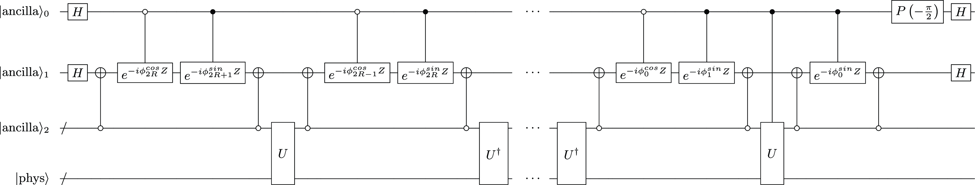


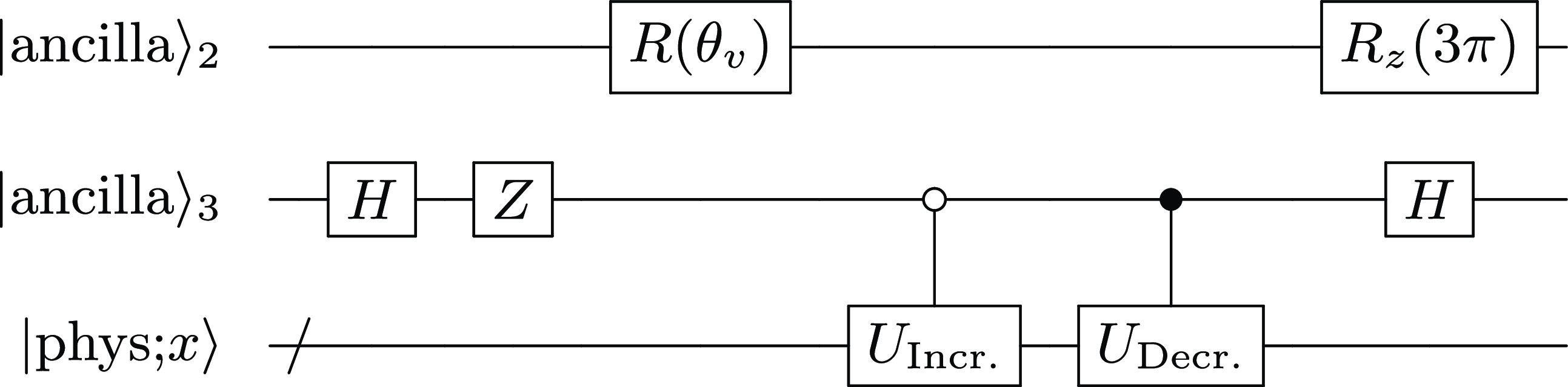


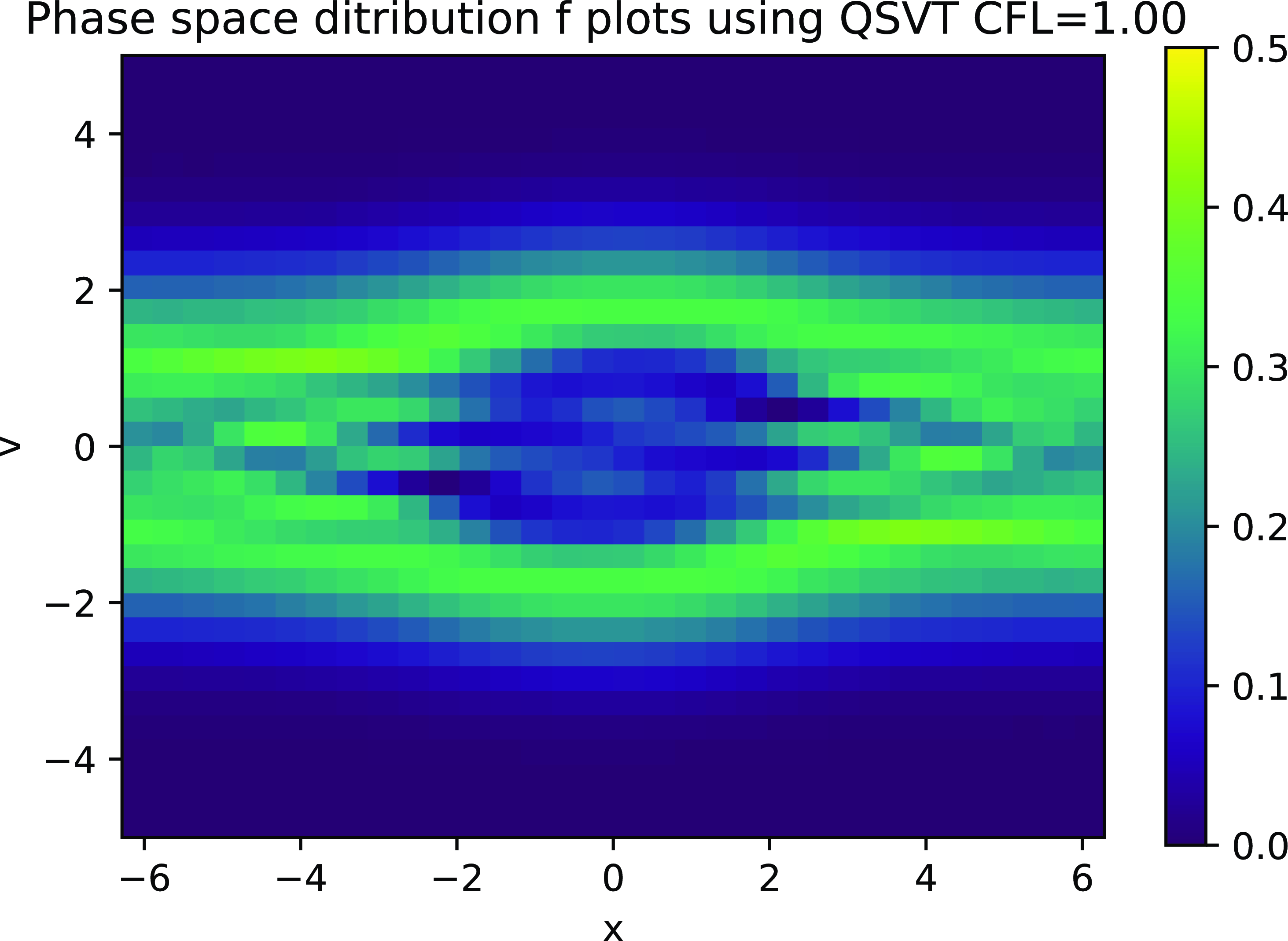


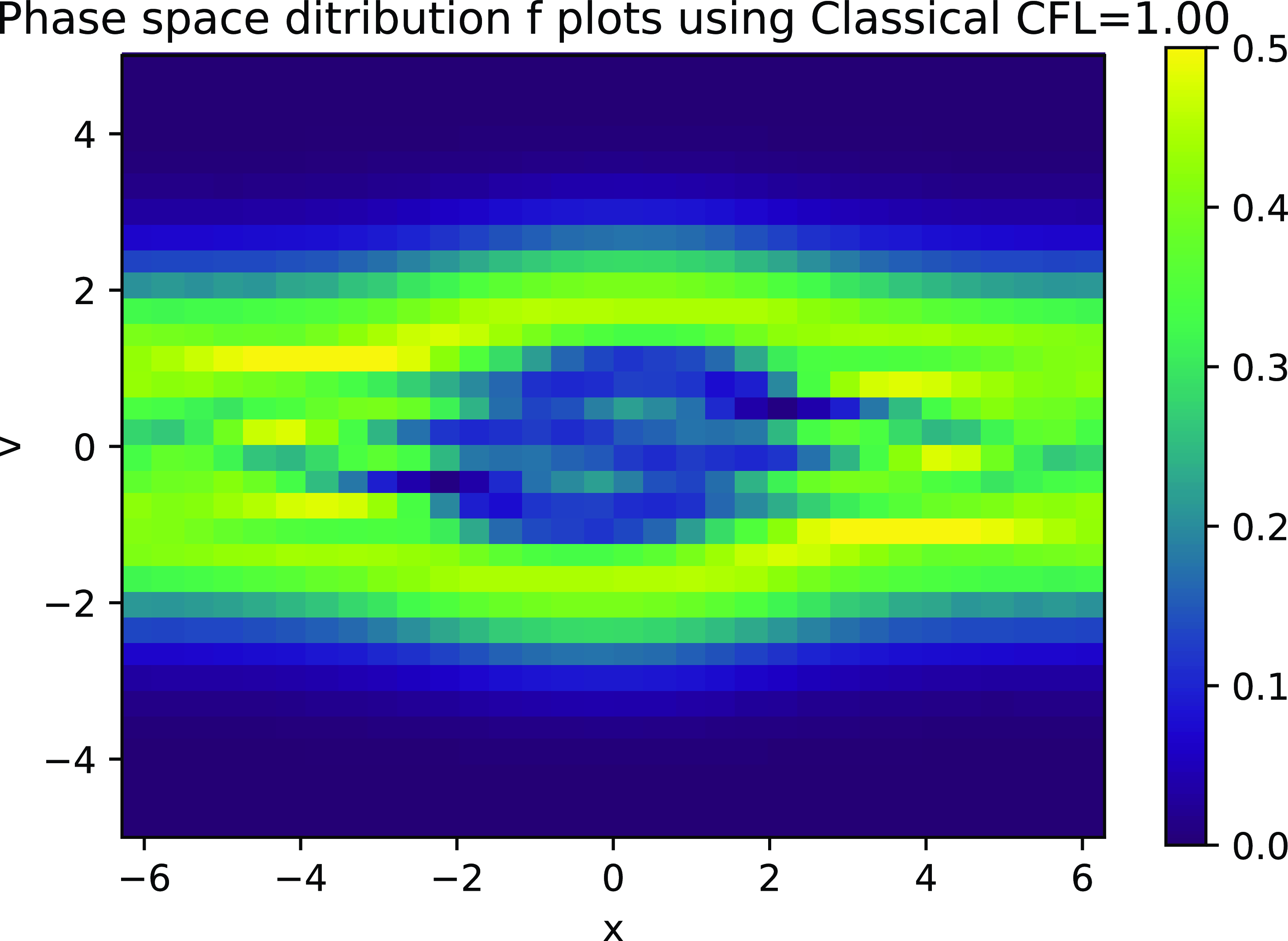


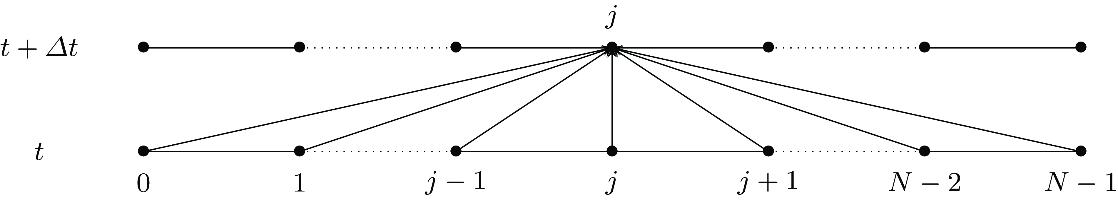


 Open access