


DISCUSSION POINTS
• Concern over climate change often leads to a pessimistic view of a future in which energy will be costly and scarce; careful consideration of the electrification of energy through free-fuel sources leads instead to an optimistic view of a future in which energy will be affordable and abundant.
• Affordability and abundance of free-fuel electricity at low penetration is no longer in doubt; it is at high penetration that the uncertainty and challenges lie.
• We can be optimistic about the many energy/information options available to an adaptive grid that could accommodate free-fuel electricity sources that fluctuate in space and time, though we do not know which of these options will be important in future.
Introduction
Consumption of energy at ever-increasing rates has been key to humanity’s improvement in quality of life. The human body itself only consumes ∼100 W. But, enhanced by modern technology, the global average human consumes ∼2.5 kW, about twenty-five times more, and the average U.S. resident consumes ∼10.3 kW, about 100 times more.1
In much conventional thinking, however, energy consumption is coupled to significant negative environmental externalities. Continued increases in the rate of energy consumption thus can seem problematic, and the resulting perspective is one of energy scarcity. Though such a perspective is a powerful motivator for increased energy efficiency, which enables humans to do more with less energy, continued increases in the global average human’s absolute rate of energy consumption are necessary for significant continued improvement in quality of life. Said differently, absence of continued increases would be at least as problematic for humanity.Reference Kelly2
In this paper, we examine three major long-term trends in energy and particularly electricity, trends which offer a more optimistic perspective, one of energy abundance and of significant increases in the rate of energy consumption and in humanity’s quality of life. A first major trend is from a world trading energy in a diversity of energy “currencies” to one whose predominant currency is electrical energy. A second major trend is from electrical energy generated from a diversity of sources to electrical energy generated predominantly by “free-fuel” sources such as solar and wind. A third major trend is from a grid in which electricity is transported unidirectionally, traded at (relatively) static prices and consumed under direct human control, to a flexible grid in which electricity is transported bidirectionally, traded at (relatively) dynamic prices, and consumed under human-tailored agential control.
We present, analyze, and discuss these trends, as well as opportunities and challenges arising when following these trends to their logical conclusions: a future in which energy is affordable, abundant, and consumed in much greater amounts than ever before. Early appreciation of these trends can accelerate them, along with the advent of an energy future which is not problematic, but instead pervasively positive.
We emphasize that our perspective in this paper is long-term and fundamental: are these trends compatible with fundamental considerations that are valid over the long term? Our purpose is not to discount also-extremely-important short-term and less-fundamental considerations, but simply to make the over-arching case that there do not appear to be fundamental reasons these trends might not continue into the long-term future. We also emphasize that our perspective is not intended to be normative (advocating for policy that favors or disfavors these long-term trends), but to be descriptive (pointing out historical trends and their compatibility with long-term and fundamental considerations).
Electrification of energy
The first long-term trend is from a world containing a diversity of energy “currencies” to one whose predominant currency is electrical energy.
In the United States, the electricity fraction of end-use energy consumption was zero in 1882, when commercial electricity generation started with a hydroelectric power plant at Niagara Falls and a coal-powered plant in New York CityReference Hausman, Hertner and Wilkins3 but has steadily and continuously grown over the last 130 years, reaching ∼30% in 2016.4 Worldwide, the fraction is slightly less (20–25%) but is nonetheless growing faster than the fraction of any other form of end-use energy consumption, as illustrated by the historical chart of Fig. 1 based on data from the United Kingdom.5
Historical trends in the percentages of various energy “currencies” consumed by end users in the United Kingdom. Electricity, the most functional of the energy currencies, has commanded a continuously increasing percentage. Note that, to the extent that the electricity is generated using one of the other fuels (coal, petroleum, natural and town gas), the total primary consumption (not just by end users) of those other fuels is higher than indicated.

This trend is certainly not over. In loose analogy to the national monetary currencies that power economic exchange, electricity uniquely has, or will soon have, all the characteristics most important for a currency that powers energy exchangeReference Rosenberg6; there is no need to invent a new and better energy currency. The characteristics of electricity, discussed below in comparison to the only other possible contender for such a near-perfect7 currency, natural gas, are that it be easily transportable, easily exchangeable into other forms of energy, and low-cost.
Transportability
The first important characteristic of an energy currency is that it be conveniently transportable all the way from point-of-creation to point-of-use, over long-haul “trunk” lines transmitting massive amounts of power as well as point-of-use “last meter” lines transmitting much smaller amounts of power.
For electricity, the state-of-the-art long-haul transport is via high-voltage DC transmission lines. At a voltage of 380 kV and a thermal-sag-limited current of ∼9 kA, a dual-conductor 2 × 3.3-cm-diameter line can transport ∼3 GW of electrical power.Reference Kiessling, Nefzger, Nolasco and Kaintzyk8 This amount of power is enormous—the equivalent of several utility-scale power plants.
For fossil fuels, long-haul transport can also be at very high rates. For natural gas, a state-of-the-art pressurized 42-inch-diameter pipeline can transport ∼500 million ft3/day of natural gas.9 Using an energy content of 1.055 MJ/ft3 and 86,400 s/day gives an effective transport rate of ∼6 GW of natural gas “power,”10 comparable to electricity transport. For coal, one 50-foot-long rail car carries ∼120 tons of coal with an energy content of ∼8.14 MW h/ton at a speed of ∼55 miles/h. Thus, the transport rate of coal “power” is ∼5700 GW.11 The time-averaged rate is of course much lower, e.g., a factor of ∼1000, if rail car utilization duty factor is considered but is nonetheless a high effective transport rate of coal “power.”
In other words, the carrying capacities of state-of-the-art long-haul electricity, natural gas and coal transport have similar orders of magnitude. The same is true for their costs, which also have similar orders of magnitude. Note, though, that their costs all have different capital, operating, and environmental (social) components,Reference Oudalov, Lave, Reza and Bahrman12 so any particular use case will depend in detail on geography, power carrying capacity, and trunk-line length. In general, trunk lines that are longer favor coal, trunk lines that are intermediate in length favor natural gas, while trunk lines that are shorter favor electricity.Reference Bergerson and Lave13
These transport rates and costs for fossil fuels are for “trunk” lines only, however—typically from point-of-origin to an electricity generating plant. At point-of-use, “last meter” fossil fuel transport is much less economical and convenient than is electricity transport. For electricity, simple 14-gauge two-strand residential wire can transport ∼1.4 kW at a capital cost of less than ∼$0.30/foot.14 For natural gas, standard 1/2″-diameter corrugated stainless steel tubing can also transport ∼1.4 kW15 but at a capital cost of ∼$1.50/foot14—a similar power carrying capacity but about 5× higher capital cost as well as with much less convenient installation procedures. For coal, there is no convenient method of point-of-use “last meter” transport.
In other words, electricity, more so than other potential energy currencies, such as natural gas and coal, is easily, flexibly, and cheaply transportable over trunk lines as well as “last-meter” wires.16,17
Exchangeability
The second important characteristic of an energy currency is that it be exchangeable efficiently and in flexibly sized units into whatever final form of energy the end-use dictates: mechanical, thermal, photonic, electrochemical, or even electrical of different voltage, frequency, or phase.
With respect to efficiency, because electrical energy is a form of potential energy, with zero entropy,18 it can be transformed with near-100% efficiency into any other form of energy without suffering from the Carnot efficiency losses (usually >50%) associated with the conversion of thermal energy into potential energy. In practice, with its inherent compatibility with electromagnetic and semiconductor technologies, electrical energy can be transformed easily and with high efficiency into all the above-mentioned forms of energy. An exception is into chemical energy, which often requires thermal activation of complex and nonselective chemical reaction pathways and outcomes.
With respect to flexibly sized units, the importance has long been noted of the availability of electromechanical power “in ‘fractionalized’ form—in small units of any required size and in a form that did not involve the wasteful generation of a large quantity of power when all that was required were small or intermittent doses.”Reference Rosenberg6 Such fractionalized power permitted in the early 20th century a reorganization of work processes that freed factory layouts from the constraints imposed by belts and shafts that were previously needed to transfer mechanical power.Reference Du Boff19
By contrast, transport and use of “fractionalized” quantities of other kinds of energy—natural gas, coal, mechanical, and thermal—is much less convenient. Particularly when end use requires intermediate conversion into heat, such as chemical to thermal to mechanical energy via a heat engine, use of fractionalized quantities of energy is not economical because of inefficiencies caused by poor size-scaling of various quantities including heat losses.Reference Peterson20
Low cost
The third important characteristic of an energy currency is that it be low cost. This characteristic is especially critical because energy is universally important, and must be universally accessible, across all of human society.
The long-term cost trends for electricity are illustrated in Figs. 2(a) and 2(b), which show the inflation-adjusted historical consumer prices of the major historical energy currencies: electrical energy, heating oil, gasoline, and natural/town gas.
(a) Long-term (1800–2014) inflation-adjusted absolute UK and U.S. consumer prices per kW h of different energy currencies versus time using purchase power parity for the conversion of UK Pence to U.S. Cents. Inspection of the figure shows a general trend of a long-term decreasing cost of most of the energy currencies, including electricity. (b) Shorter term (1960–2014) inflation-adjusted U.S. consumer prices of different energy currencies versus time (expressed in 2015 U.S. Cents). The shorter-term price of electricity has been decreasing whereas that of other energy currencies has been increasing.

The top Fig. 2(a) shows the longer-term (1800–2014) historical evolution of the prices of those energy currencies. The figure includes (i) historical data back to 1900 from the United Kingdom5 and (ii) data back to 1960 from the United States. Although taxation rates in the United Kingdom and the United States are different (and are reflected in the figure), the evolution of the prices of the different energy currencies in the two countries is remarkably consistent. Each of the energy currencies, upon introduction, underwent an initial decrease in price. Electricity, as the most recent, underwent the most recent initial decrease in price.
Fig. 2(b) shows a shorter-term (1960–2014) historical evolution of the prices of energy currencies based on data21 made available by the U.S. Energy Information Administration (EIA). Inspection of the figure reveals opposite trends in the evolution of the prices of electrical energy versus prices of other forms of energy. While the inflation-adjusted price of natural gas, gasoline, and heating oil has generally been constant or increasing, the price of electricity has decreased by 40% over the last 50 years.
At present, the price of electricity is approximately three times the price of natural gas. This makes sense in the context of non-free-fuel electricity generation: electricity is currently predominantly generated by burning natural gas; the efficiency of utility-scale conversion from natural gas to electricity is about 1/3; thus, the price of electricity can be expected to be about 3× that of natural gas per unit of energy content.22 However, in the longer term, as discussed below, electricity predominantly generated from free-fuel sources will enable even lower electricity prices. Thus, in the context of non-free-fuel electricity generation, the price of electricity will at most be about 3× the price of natural gas. In the context of free-fuel electricity generation, the price of electricity is likely to become much lower.
Moreover, the “effective” price of electricity for many uses is not 3× that of C-chemistry–based fuels. For example, the conversion efficiency of the energy in C-chemistry–based fuels to mechanical energy (e.g., in transportation’s internal combustion engine) is typically 1/4, making the effective price of electricity for transportation ∼3/4 the price of gasoline.23 Or, for example, the conversion of the energy in C-chemistry–based fuels to thermal energy (e.g., for space or water heating) is, using modern gas furnaces or boilers, about 0.9, while the coefficient of performance for heat pumps which use electricity to transfer thermal energy is approximately 3× (albeit under moderate temperature conditions), making the “effective” price of electricity for heating about 0.9 = 0.9 (3/3) the price of natural gas. In other words, the price of electricity is generally already comparable if not lower than the price of C-chemistry–based fuels per unit energy delivered in the desired form.
Free-fuelification of electricity
The second long-term trend is from electrical energy generated by a diversity of sources to electrical energy generated predominantly by free-fuel sources. What do we mean by “free-fuel” sources? Free-fuel sources of electricity are sources for which no fuel needs to be purchased: e.g., wind, water, solar (WWS), and geothermal.24 But free-fuel sources are by no means synonymous with “renewable” sources, as these include sources for which fuel is not free: e.g., biomass or biofuels whose production and transport25 must be purchased. The reason we emphasize here “free-fuel” sources is because, as discussed below, the price of electricity from these sources is limited mainly by the harvesting technology, not by the price of the fuel, thereby providing a fundamental advantage and potential to decrease radically in price.
Indeed, free-fuel electricity generation has been increasing very rapidly during the past two decades. The left panels of Fig. 3 show a sixty-five-year history of annual U.S. electricity generated from all sources, including free-fuel sources, along with the total annual U.S. electricity generated. Wind electricity has been doubling every two years, an exponential growth rate, and is projected to exceed hydroelectricity within a few years.26 Similarly, solar electricity has been doubling every year, an even higher exponential growth rate that might enable it ultimately to exceed both hydroelectricity and wind.27 Although not shown in Fig. 3, geothermal electricity generation also has significant potential, particularly with deep (10 km) “enhanced geothermal” technologies on the horizon.Reference Tester, Anderson, Batchelor, Blackwell, DiPippo, Drake, Garnish, Livesay, Moore, Nichols and Petty28
Historical development of the generation of electric energy in the United States, on linear (a) and logarithmic (b) scales. In the United States, the annual electric energy generated by wind energy is expected to exceed hydroelectric energy in a few years. Historical development of new electricity generating capacity, both total (c) and broken out by free-fuel (d) and non-free-fuel (e) sources.

These rapid growth rates are consistent with recent data on electricity generation capacity added in the United States. As illustrated in the right panels of Fig. 3, a higher 2016 new generation capacity is anticipated for free-fuel than non-free-fuel generation sources: 64% of new generation capacity added in 2016 was from free-fuel sources, dominated by solar (9.5 GW) and wind (6.5 GW); while only 36% of new generation capacity added in 2016 was from non-free-fuel sources, dominated by natural gas (8 GW).29
Of course, these new generation capacity additions may be influenced by government subsidies and incentives. And the absolute amount of electricity generated from free fuels (11%) is still small compared to that from non-free-fuels (89%). But exponential-growth curves are powerful, and even if their growth slows (as it inevitably must), current trends suggest a long-term future in which electricity is dominated by free-fuel sources. Still, for this trend to continue, the prices of electricity from free-fuel sources must (i) continue to decrease and, if electricity itself is to become the dominant energy currency, free-fuel sources must (ii) be abundant enough to fulfill the vast majority of the world’s energy needs. We discuss these two topics next in sections “Steadily decreasing ‘low-penetration’ cost of free-fuel electricity” and “Abundance limit to free-fuel electricity is more than a century away”.
Steadily decreasing “low-penetration” cost of free-fuel electricity
Regarding the price of electricity generated from free-fuel sources, we first discuss the “low-penetration” cost—the cost of generating the electricity then adding it to the grid at low (<50%) penetration. We discuss later (in section “Making the grid adaptive”) the “high-penetration” cost of generating the electricity when adding it to the grid at high (>50%) penetration, which will be higher because of the need to mitigate “lumpiness” of electricity generation in time and space.
The historical trends for the low-penetration cost of solar and wind electricity are illustrated in Fig. 4. To make comparison with end-use consumer prices for other sources of electricity, we plot calculated and projected levelized costs of electricity (LCOEs)—basically a life-cycle cost that includes operating (Opex) costs as well as capital (Capex) costs of harvesting technologies amortized over their lifetimes. Note, since LCOE calculations and projections generally contain significant uncertainties, including discount and interest rates, we plot the LCOEs from a number of literature sources.30
LCOE, both actual and projections, for solar and wind, compiled from various sources. ASPs in the United States are also indicated; from 1980 to 2009, based on data published by Lazard (2014), the LCOE for solar photovoltaics exceeded 300 US$/MW h, as indicated by the horizontal orange bar at the top. LCOEs are beset with uncertainties that include future interest rates and payments that are part of the capital expenses (Capex). By contrast, ASPs do not include such uncertainties. Accordingly, the (estimated) LCOEs and the (precise) ASPs can be (substantially) different. Furthermore, given that the LCOE includes uncertainties, there are inevitably differences amongst the LCOE values originating from multiple literature sources. These differences are consistent with the spread of data displayed in the figure.

Inspection of Fig. 4 reveals that the LCOEs of both solar and wind electricity are decreasing rapidly, suggesting room for continued decrease. This is not the case for non-free-fossil-fuel electricity. An important reason for this is found in the fact that for non-free-fuel electricity, the major or even dominant cost of the electricity is the fuel itself. Indeed, a detailed analysis of the historical development of the LCOE of coal-fired power plants has shown that the cost of fuel is the single largest (40–60%) expense.Reference McNerney, Doyne Farmer and Trancik31 And, since coal and natural gas are comparably priced [see Fig. 2(a)], even with the recent fracking-enabled decreases in the cost of natural gas,Reference Mason, Muehlenbachs and Olmstead32 fuel is the dominant expense for all fossil-fuel–based power plants.
By contrast, for free-fuel electricity, instead of the cost of fuel, it will be the capital investment in harvesting technology that is the dominant expense.Reference Smil33 These may have their own fundamental cost limits, but can be anticipated to be subject to relentless technology improvement rather than by the geopolitics and scarcity of fuel.
Indeed, if technology improvement on the electricity generation side is anything like that on the electricity usage side, the room for further cost reduction is considerable. The dominant cost of virtually all energy services (lighting, heating, cooling, and transportation) is not for the capital expense of the appliance itself (Capex) but for the operating expense of the fuel (Opex). In other words, relentless improvements in technology drive down appliance costs until they are no longer dominant. In general lighting, for example, traditional incandescent, fluorescent, and high-intensity-discharge lamps and fixtures (the “appliance”) represent approximately 1/3 of the cost of lighting, while electricity (the “fuel”) represents approximately 2/3.Reference Tsao and Waide34 Rapidly evolving solid-state lighting is heading for a very similar cost structure, even while adding many new performance features.Reference Tsao, Crawford, Coltrin, Fischer, Koleske, Subramania, Wang, Wierer and Karlicek35,36
In other words, since technology advance rather than fuel “mining” becomes cost determinative, there is significant room for continued decrease in the cost of free-fuel electricity. Thus, the impending transition to free-fuel generation sources “breaks” the linkage between the price of electricity and the price of the fossil fuels that historically have been used to generate electricity. As mentioned in section “Low cost”, in the recent past, the price of electricity (per kW h generated) has been 3× that of fossil fuels (per kW h energy content) since fossil fuels have been the dominant electricity generation method. Looking forward, the price of electricity can and presumably will be less than 3× that of fossil fuels, perhaps much less, as the price of free-fuel electricity generation continues to decrease.
Irrespective of these considerations, and keeping in mind that LCOE is a calculated cost, the true test of the viability of free-fuel generation sources is the actual price paid for the electrical energy, i.e., the average selling price (ASP) for 1 MW h. Inspection of Fig. 4 reveals that the ASPs (in the United States) of both solar and wind electricity have been decreasing steadily, are now of the order US$25–40/MW h,37 and hence are more than competitive with the cost of non-free-fuel sources. One might even expect solar and wind electricity prices ultimately to approach those of free-fuel-based hydroelectricity, at present the lowest cost generally available electricity.38
Abundance limit to free-fuel electricity is more than a century away
Regarding the maximum abundance of electricity generated from free-fuel sources, wind and solar energy combined are believed to be capable of supplying humanity’s consumption of electricity well into the next century. For wind alone, some estimates are as high as 5× of all global energy consumed in 2007,Reference Lu, McElroy and Kiviluoma39,Reference Archer and Jacobson40 though these estimates are likely high because they do not, among other things, account for incomplete replenishment of solar energy into the wind at high harvesting rates.Reference Miller and Kleidon41–Reference Wallace and Hobbs43
Perhaps more importantly, for solar, the limits are even higher. Indeed, superficially the supply of solar electricity seems nearly unlimited: the sun delivers to the earth in 1.8 h the energy consumed by all humanity in the year 2012,Reference Tsao, Lewis and Crabtree44 and thus the solar resource seems roughly 5000 ≈ (1 year)/(1.8 h) times larger than current human needs.
However, harvesting of solar electricity on a global scale would alter the earth–sun radiation balance, hence would not be global-warming-neutral. The earth’s land surface albedo, the fraction of the solar power incident on the earth’s land surface that on average is reflected, is αland ∼ 0.26. Harvesting of solar energy on land thus means on average replacing surfaces of such intermediate albedo with surfaces of near-zero albedo, thereby reducing the earth’s overall albedo. A reduced albedo implies a higher absorption of solar power by the earth, and thus implies a higher earth temperature necessary to reradiate that solar power and restore the earth–sun radiation balance.Reference Hu, Levis, Meehl, Han, Washington, Oleson, van Ruijven, He and Strand45
Based on well-established treatments of the earth–sun radiation balance,46 the degree to which the earth’s temperature must be higher as a consequence of the artificial human harvesting of solar power can be given as
 $${{\Delta {T_{{\rm{earth}}}}} \over {{T_{{\rm{earth}}}}}} = \left( {{{{\alpha _{{\rm{land}}}}{f_{\rm{a}}}} \over \varepsilon }} \right)\left( {{{{S_{\rm{o}}}} \over {{S_{{\rm{surf}}}}}}} \right){{\Delta {P_{{\rm{earth}}}}} \over {4{P_{{\rm{earth}}}}}}.$$
Up to an order-unity correction factor, (αlandf a/ε)(S o/S surf), the fractional increase in the earth’s temperature (ΔT earth/T earth) is one fourth the artificially harvested solar power (ΔP earth) that the fractional increase in the earth’s temperature would enable to be radiated, itself as a fraction of the blackbody power radiated by the earth into space (P earth) in the absence of artificially harvested solar power. The various terms in the correction factor in Eq. (1) are as follows: the earth’s land surface albedo (αland),Reference Wild, Folini, Hakuba, Schär, Seneviratne, Kato, Rutan, Ammann, Wood and König-Langlo47 the solar harvesting efficiency (ε),Reference Leite, Woo, Munday, Hong, Mesropian, Law and Atwater48 the proportional change in planetary albedo per change in land surface albedo (f a),Reference Lenton and Vaughan49 and the ratio between the solar flux at the top of the atmosphere and the land surface (S o/S surf)Reference Trenberth, Fasullo and Kiehl50
Using the numerical values listed in the endnotes, the correction factor becomes (αlandf a/ε)(S o/S surf) ∼ 0.46. The quantitative implication is that, if we wish to limit the earth’s temperature rise to a negligible ΔT earth ∼ 0.2 K on a base of T earth ∼ 288 K, then artificially harvested solar power would need to be limited to ΔP earth ∼ 600 TW on a base of P earth ∼ 100 PW. This is about 30× larger than the power consumed by humanity in 2012. If one projects the past 100 years of energy consumptionReference Smil51 into the future, as illustrated in Fig. 5, this consumption would not be reached until the year 2170, about 150 years from now, and is thus consistent with a future in which humanity can largely be fueled by solar electricity.Reference Ahn, Cowern, Han and Lee52 It is, however, certainly not infinite. Depending on the growth rate of humanity’s power needs, sometime next century albedo-preserving methods for artificially harvesting solar power, or alternative sources of power, might be necessary. For example, the earth’s land surface albedo could be preserved by balancing the absorbing black solar-cell surfaces with reflecting white surfaces (such as white-colored roofs); or solar power could be preferentially harvested over the oceans, whose albedos are very low.Reference Reindl and Schmaelzle53
World consumption of artificial power. Data [orange circles, after V. Smil, “Energy transitions: history, requirements, prospects” (ABC-CLIO, 2010)] are estimates over the past two centuries; projection into the future (dashed blue line) is based on a fit to the past century’s data. In 2170, humanity’s world artificial power consumption projects to be ∼0.6 PW, which is the point at which the earth’s temperature rise, if this consumption was totally from solar power absorbed by the earth due to artificial harvesting (ΔP earth), would no longer be negligible.

Making the grid adaptive
The two trends discussed above paint an optimistic scenario: a world in which the predominant energy currency, electricity, is transportable, exchangeable, and low-cost, and in which electricity is predominantly generated from free-fuel sources with the potential for continuing decreases in the cost of energy and for supplying humanity’s long-term energy needs, possibly for the next century and a half.
However, with respect to low-cost, we only discussed above the “low-penetration” cost of free-fuel electricity. The “high-penetration” cost is also critically important but is much higher due to the cost of accommodating the fluctuations of the supply of and demand for electricity in space and time (“lumpiness”). This cost already exists, of course, because of demand fluctuations which force the supply of relatively expensive “peaking” power. But the cost becomes much more significant with free-fuel electricity, as solar or wind electricity can only be generated when sun or wind are present, and supply fluctuations are added to demand fluctuations, both in time and space.
The fluctuations in time are illustrated by the “Duck Curve”Reference Denholm, O’Connell, Brinkman and Jorgenson54 in Fig. 6(a). To some extent, solar electricity is synchronous with daily and yearly systematic variations in electricity demand, that is, solar electricity can sometimes be most plentiful when needed most, during mid-day and during the summer period when air conditioning is desirable. But, as seen in the “Duck Curve”, the remaining variations and fluctuations are large and must be managed. Moreover, the cost of managing these will increase super linearly with increasing fraction of electricity generated from free-fuel sources.Reference Frew, Becker, Dvorak, Andresen and Jacobson55
(a) A “duck” curveReference Denholm, O’Connell, Brinkman and Jorgenson54 illustrating the forecasted hourly mismatch in California, from midnight to midnight, between the total demand for electricity, and the anticipated supply of solar electricity, as the projected penetration of solar electricity increases from 2013 to 2020. During the mid-day hours, from 10 am until 4 pm, the solar resource is high, so demand-minus-supply is lowest (the belly of the duck). During the early evening hours, from 6 pm until 8 pm, residential demand spikes but the solar resource is low, so demand-supply is highest (the head of the duck). During the late evening and early morning hours, from 10 pm until 9 am, demand is low and the solar resource is also low, so demand-minus-supply is moderate (the tail of the duck). Licensed with permission from the California ISO (Independent System Operator). (b) A “heat map” of the geographic variation of the solar resource in the United States. The regions of high solar resource (high solar electricity supply) do not generally overlap the regions of high population density (high electricity demand). The map was created by (and reproduced here courtesy of) the National Renewable Energy LaboratoryReference Roberts56 for the U.S. Department of Energy.

The fluctuations in space are illustrated by the “heat map”Reference Roberts56 in Fig. 6(b). Some regions, such as California, with plentiful solar resource (high supply) coincide with high population density (high demand). But many regions, such as the Northeast United States, have scarcer solar resource (low supply) and high population density (high demand).
Moreover, to these more predictable supply and demand fluctuations in time and space must also be added those that are less predictable, including those due to accident, war, or terrorism, or even normal uncertainties in peaceful human activity.
The solution to the accommodation of these fluctuations must lie in an adaptive grid, the coming dual network of energy and information flow that unleashes pricing and market forces to optimally and dynamically facilitate the matching of energy supply and demand. The third long-term trend, then, is the grid becoming more adaptive: from a grid in which electricity is transported unidirectionally, traded at (relatively) static prices, and consumed under direct human control; to a grid in which electricity is transported bidirectionally, traded at (relatively) dynamic prices, and generated and consumed under human-tailored agential control.
Note that what we mean by “adaptive” goes beyond what is conventionally meant by “smart.” Specifically, we mean to include the energy sources and sinks as well as the energy flow (transmission) technologies; and we mean to include the information-processing agents as well as the information flow technologies. We mean a grid whose energy sources and sinks self-organize into an energy market that mediates energy generation and use on behalf of human needs, much as financial markets self-organize so as to mediate the generation and use of goods and services on behalf of human needs.
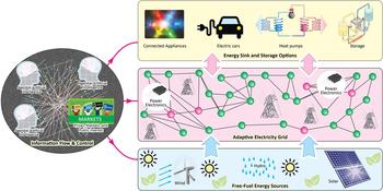
We are optimistic about two classes of technologies, both necessary to an adaptive grid. The first class are energy technologies which give the adaptive grid energy source and sink options for the flexible matching of energy supply and demand.Reference Jacobson, Delucchi, Cameron and Frew57 The second class are technologies which give the adaptive grid the ability to facilitate the energy and information control and flow required to optimally and dynamically match energy supply and demand (Fig. 7).
Two classes of technologies necessary for making the grid adaptive so as to manage the lumpiness in space and time of free-fuel electricity. On the right, an adaptive electricity grid (middle in pink) facilitates energy flow from free-fuel energy sources (bottom in blue) to energy sink and storage options (top in yellow). On the left, agential artificial intelligences direct the trading of electricity so as to arbitrage away price differences created by demand/supply variation in time and space.
In this Section, we briefly discuss these two classes of technologies. We do not set economic or performance targets for them, so do not estimate and compare how near or far these technologies are from practical application, though such targets would be of great interest to develop.58
Energy source and sink options
The first class of technology necessary for the adaptive grid are energy sources and sinks which will give the adaptive grid options for the flexible matching of energy supply and demand. The most important of these are production overcapacity, storage, and “connected” appliances.
Production overcapacity
One important energy source is simply the free-fuel source of electricity itself. The continuing decrease in the cost of electricity generated from such sources may allow for a generation-infrastructure overcapacity that buffers the variation in fuel availability in time and space. In other words, in the limit of cheap electricity, “lumpiness” of electricity can be alleviated, to some degree, by production overcapacity. That is, the lowest production capacity can be matched to the highest consumption rate, and when consumption rates are lower, production can be “curtailed.” Such curtailment is often viewed negatively, but if the energy source is sufficiently inexpensive, some amount of curtailment is economically optimal.Reference Jacobsen and Schröder59
Storage
An important energy source and sink is storage, which can alleviate lumpiness of electricity in time. Though historically storage has been electricity’s Achilles Heel, much progress is being made.
First, the cost of Li-ion rechargeable batteries has decreased so much that the levelized cost of storage of electricity at a utility scale is now in the order of US$0.27–0.56/kW h,60 still higher than the cost of the electricity itself, but by less than 3–6×.
Second, because of the many performance advantages of electrified transportation, an enormous infrastructure of rechargeable batteries will be created in the coming decades, which might be co-opted for storage of grid electricity.
Third, competitors to Li-ion batteries are on the horizon, including chemical storage based on fuel and flow cells, and on hydrogen.
Fourth, although water and other forms of mechanical potential energy storage depend on local geography and will not be equally available globally, where it is available, it can be quite powerful as demonstrated by its integration into the three-nation Norway–Denmark–Germany grid in which Norway provides hydropower to complement Denmark’s wind and Germany’s solar power.
We emphasize that, though much progress is being made, it is as yet unclear whether many practical challenges can be overcome, including in the long-term the sheer magnitude of energy storage (and of the materials used for energy storage) that may be necessary. We note, though, that storage is but one of the three options discussed here for the flexible matching of energy supply and demand, so the magnitude of energy storage might well be lower than currently thought necessary.
Connected appliances
Perhaps the most important “sink” for electricity is appliances—broadly defined, these are the “actuators” that serve humanity. If one includes amongst these all residential, office, industrial, and outdoor grid-connected services such as heating, cooling, lighting, cooking, washing, cloud computing, and data storage, Internet-of-Things devices—very quickly, a large fraction of all energy demand is captured.
Importantly, all of these grid-connected appliances have considerable flexibility in when and how intensely they can be used: they can be “load scheduled.” Warm or cool air can be stored in unused rooms and zones in a building then vented to used rooms and zones as needed. The human eye has a logarithmic response to light intensity, so lumen levels in various rooms and zones in a building can be almost unnoticeably increased or decreased to accommodate real-time fluctuations in the price of electricity.
The key is that these appliances be connected not just to the energy grid but to the information grid that will enable their use to be intelligently managed. In the artificial lighting case mentioned above, a new generation of smart,Reference Schubert and Kim61 connectedReference Tsao, Crawford, Coltrin, Fischer, Koleske, Subramania, Wang, Wierer and Karlicek35 lighting is enabling exactly this.
Energy and information flow and control
Given energy sources and sinks which will give the smart grid options for the flexible matching of energy supply and demand, a second class of technology is also necessary for the adaptive grid: that which facilitates the energy and information flow and control required to optimally match intermittent energy supply and demand. Indeed, on a larger scale, energy and information are likely to become so profoundly interconnected in future that the term “information-energy nexus” may be appropriate. Similar to the so-called “water-energy nexus,”62 the impact will be bidirectional: we will need information tools to manage electrification and the smart grid; at the same time, information tools in general will increasingly consume huge amounts of electricityReference Schulte, Welsch and Rexhäuser63—by some estimates as much as 9–51% of all electricity by 2030.Reference Andrae and Edler64
Energy flow: long-distance electricity transport
One key aspect of fluctuations is that they themselves vary over geography. On a very large geographical scale, seasonal fluctuations depend on hemisphere and latitude, and daily fluctuations depend on longitude. On smaller geographical scales, real-time fluctuations due to weather (cloudy skies, calm air) depend on local (meters to kilometers to hundreds of kilometers) position.
Because the fluctuations vary over geography and over different length scales, there is a great advantage to being able to transport electricity and average out the fluctuations over the largest possible geographical areas. Very approximately, if the standard deviation of the fluctuations in electricity generation is σo in an area A o, and if the amplitude and phase of the fluctuations across contiguous such areas were random, then the standard deviation of the fluctuations in electricity generation σ over larger areas A would scale as σ = σo × (A o/A)1/2. In other words, the fluctuations in electricity generation decrease as 1/√A. The decrease is sublinear and reduced by correlations in the variations across contiguous areas,Reference Kahn65 but is nonetheless significant.Reference Archer and Jacobson66,Reference MacDonald, Clack, Alexander, Dunbar, Wilczak and Xie67
This general idea is one motivation for a globe-spanning “SuperGrid”Reference Gellings68 that would enable global scale averaging of fluctuations, not to mention unleashing the full economic benefits of geographic specialization of electricity production (the sunniest areas specializing in solar electricity, the windiest areas in wind electricity). Indeed, though continued innovations in high-voltage DC transmission technology are likely necessary, one might argue that such a SuperGrid is already economically viable.Reference Blarke and Jenkins69 The challenges are more at the system level: how to maintain reliability even in the presence of large-scale unintentional (accidents) or intentional (terrorism or war) events; and how to allocate economic return to infrastructure investments that cross political borders.
Energy control: power electronics
As discussed above, electricity has an inherent intimate compatibility with electromagnetic and semiconductor technologies. It also comes in various “formats”: voltages, currents, and waveforms (AC, DC). Mediating the bidirectional flow and interconversion of electricity between formats is the domain of power electronics, the class of semiconductor technologies that switches and controls high voltages and high currents.
Power electronics based on Si is already well developed, with much ongoing development on wider band gap semiconductors such as SiC and GaN for higher voltage higher current switching. On the horizon are ultra-wide-bandgap semiconductorsReference Tsao, Chowdhury, Hollis, Jena, Johnson, Jones, Kaplar, Rajan, Van de Walle, Bellotti, Chua, Collazo, Coltrin, Cooper, Evans, Graham, Grotjohn, Heller, Higashiwaki, Islam, Juodawlkis, Khan, Koehler, Leach, Mishra, Nemanich, Pilawa-Podgurski, Shealy, Sitar, Tadjer, Witulski, Wraback and Simmons70 such as AlGaN/GaN, diamond, and Ga2O3. Among the challenges are not only to increase open-circuit voltages (standing off high voltages when the switch is off) and closed-circuit currents (conducting high currents when the switch is on), but also to decrease losses to a level where thermal dissipation and heat sinks no longer limit subsystem and system performance and design. For example, it has been suggested that neighborhood MW-class power transformer stations, currently school-bus-sized behemoths weighing 4500 kg or more, might be replaced with suitcase-sized switched power converters weighing only 450 kg (a “sub-station in a suitcase”).71
Ultimately, semiconductor power electronics may bring performance and cost advantages to switching and voltage conversion throughout the grid, all the way from high-capacity trunk lines at 100’s of kV (using transistor stacks) to low-capacity local lines at 1’s of V. This trend would only be accelerated as the convenience and flexibility of DC electricity is increasingly recognized.72
Information control: agential artificial intelligence
It is one thing to have the hardware that transports, switches, and converts electricity over distances both short and long (m to 1000 s of km). It is another thing to have the software, or “smarts,” to control that transport, switching, and conversion. Such smarts must enable a market-based matching of electricity supply and demand via the real-time negotiation of the hundreds of millions, even billions, of energy-producing and consuming agents (prosumers) that will ultimately comprise the growing Internet of “Energy-Things”.
Humans of course cannot do this negotiation; they do not have the necessary real-time smartness. Instead, they must have software agents, smart agents, to negotiate on their behalf—agents that have artificial intelligence of some form.Reference Ramchurn, Vytelingum, Rogers and Jennings73
The agents must learn from past behavior to anticipate future behavior. They must learn the detailed behavior of their own patch of the network: at what times, for instance, is a given household’s electric vehicle (potentially both a form of transport and a temporary energy storage unit) likely to be a load on, or a supply into, the grid? They must also learn the behavior of other agents they are likely to negotiate with: at what times, for instance, will other agents be likely to have not enough energy and at what other times to have surplus energy?
The agents must cooperate and compete with other agents, and so must have both information about other agents’ negotiating positions (price, production, consumption) and meta-information about their trustworthiness. Some agents will aggregate and negotiate aggregately, leading to a hierarchically aggregated (modular) architecture.Reference Simon74 Some aggregate agents will publish and guarantee their future intentions to other agents on various time scales (minutes, hours, days, weeks, months, perhaps even years)—a predictability that other agents may value and pay for. Some agents will be simply intermediaries that scour the network looking for inefficiencies that they can arbitrage away and profit from: tracking, e.g., commercial, industrial, and municipal energy usage and automatically charging/discharging energy from storage to shave peak demand.Reference Brazell75
Interestingly, exactly these kinds of artificially intelligent agents are already being developed for other purposes, so it is entirely possible that very little additional investment will be needed for adaptive-grid agents.Reference Russell, Dewey and Tegmark76
Information control: prices, markets, and the public interest
Mediating agential negotiation will be prices and the markets (both current and futures) that form around those prices. Perhaps most important will be the rules that govern those markets, rules that must ensure fairness to the agents, but also that represent the public interest. For example, the reliability and robustness of the network against unintentional or intentional perturbations is important to all agents. Policies which protect against network failure must be present, either via pricing or regulatory signals.
Indeed, many of the public interest issues present for the smart grid also arise for other domains such as water distribution, transportation, telecommunication, even financial networks where large numbers of heterogeneous entities act and interact. Hence, there is potential to borrow technologies across these domains and also address broader issues that affect the sustainability of such systems in a unified manner: cybersecurity; the ethics of delegating human decision making to artificially intelligent systems; the use of insurance mechanisms to guarantee various levels of reliability; and the possible existence of natural transmission and distribution monopolies (utilities).
To best design policies that protect the public interest, it will be important to design simulation systems that can accurately represent both the grid and the behaviors of prosumers, to predict the emergent properties of the system under a range of different conditions (e.g., weather patterns or social activities) and worst-case scenarios (generators failing or circuits tripping). Perhaps we have the opportunity to construct an energy marketplace that learns from, and goes beyond, current financial marketplaces in protecting the public interest. Note, though, that electricity markets are very different from (and more challenging than) other markets in that they have the requirement of absolute and real-time supply/demand balancing.
Finally, we note that energy markets are a complex mix of highly regulated public and private interests, so a redesign of the price and market “rules” that agents use to negotiate amongst themselves on the adaptive grid will not be trivial. They will require overcoming significant institutional and public policy inertia.
Conclusions
We have discussed in this article three major trends: electrification of energy, free-fuelification of electricity, and making the electrical grid adaptive to handle the lumpiness of electricity supply and demand in space and time. Though not without many significant practical challenges, there appear to be no fundamental technological barriers to the continuation of these trends into the future—not just in the United States, whose data were used to illustrate the trends, but worldwide and thus for all of humanity. The result would be no less than a remaking of humanity’s energy landscape into one in which energy is affordable, abundant, and efficiently deployed across all of human society.
The primary benefit would be economic: a continuation of the increase in economic productivity and wealth of human society.Reference Smalley77,Reference Smil78 But there are also important secondary geopolitical and environmental benefits.
Geopolitically, perhaps the most important benefit will stem from the diversification of energy economic “power” along a geographic dimension, as free-fuel resources (e.g., solar, wind) are much more evenly distributed geographically than non-free-fuel (e.g., fossil-fuel) resources.Reference Scholten and Bosman79 The diversification will help reduce energy-based concentrations of geopolitical power and vulnerability,Reference van de Ven and Fouquet80 likely reducing incentives toward global conflict and warReference Caselli, Morelli and Rohner81; and will also be more conducive to local infrastructure and behavioral adaptation, thus reducing the risk of locking economies into non-optimal energy-usage pathways.Reference Fouquet82 Some diversification might also take place along a market dimension, as electricity producers, consumers, and arbitragers all become information-rich actors and market participants. However, such diversification might not lead to a reduction in corporate power concentration.Reference Coady, Parry, Sears and Shang83 Instead, corporate power might simply shift from energy-resource corporations to technology corporations whose economies of scale enable them to more efficiently manage particular pieces of the energy and information producer/consumer/arbitrager network.Reference O’Sullivan, Overland and Sandalow84
Environmentally, the benefits are associated with the cleanliness of free-fuel–based electricity. The cleanliness is in part direct, in that free-fuel sources have minimal local externalities compared to fossil fuel sources (oil and gas exploration and production, e.g., has been responsible for twenty percent of all nonhazardous waste produced in the United StatesReference O’Rourke and Connolly85). The cleanliness is also indirect, in that very little CO2 is produced as a by-product, and thus will have no or negligible impact on climate.
Acknowledgments
We are grateful for helpful comments from Eugene Tsao, George Crabtree, Martin Green, Aixue Hu, Isik Kizilyalli, Jeff Koplow, Murat Okandan, Ali Pinar, and Vaclav Smil, though remaining errors are of course the responsibility of the authors. Sandia National Laboratories is a multimission laboratory managed and operated by National Technology and Engineering Solutions of Sandia, LLC, a wholly owned subsidiary of Honeywell International, Inc., for the U.S. Department of Energy’s National Nuclear Security Administration under contract DE-NA0003525.


