


1. Introduction
Turbulent flows are ubiquitous in nature, filling the gap between smooth (deterministic) and random motion. Their Eulerian properties, described by the velocity vector field
 $\boldsymbol{v}(\boldsymbol{x},t)$
and its space–time statistics, are often easy to measure, simulate and interpret. In contrast, Lagrangian characteristics are significantly more challenging to capture (especially in fusion plasmas) and have been the subject of an extensive body of research over the past century being described by the statistics of particle trajectories
$\boldsymbol{v}(\boldsymbol{x},t)$
and its space–time statistics, are often easy to measure, simulate and interpret. In contrast, Lagrangian characteristics are significantly more challenging to capture (especially in fusion plasmas) and have been the subject of an extensive body of research over the past century being described by the statistics of particle trajectories
 $\boldsymbol{x}(t|\boldsymbol{x}_0)$
and associated Lagrangian velocities
$\boldsymbol{x}(t|\boldsymbol{x}_0)$
and associated Lagrangian velocities
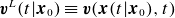 $\boldsymbol{v}^L(t|\boldsymbol{x}_0)\equiv \boldsymbol{v}(\boldsymbol{x}(t|\boldsymbol{x}_0), t)$
. The relation between these two is the V-Langevin equation (Balescu Reference Balescu2007):
$\boldsymbol{v}^L(t|\boldsymbol{x}_0)\equiv \boldsymbol{v}(\boldsymbol{x}(t|\boldsymbol{x}_0), t)$
. The relation between these two is the V-Langevin equation (Balescu Reference Balescu2007):
 \begin{eqnarray} \frac{\text{d}\boldsymbol{x}(t|\boldsymbol{x}_0)}{\text{d}t} = \boldsymbol{v}(\boldsymbol{x}(t|\boldsymbol{x}_0), t) \equiv \boldsymbol{v}^L(t), \quad \boldsymbol{x}(0|\boldsymbol{x}_0) = \boldsymbol{x}_0. \end{eqnarray}
Monin (Reference Monin1971) revealed that Eulerian velocity fields
 $\boldsymbol{v}(\boldsymbol{x}, t)$
that are homogeneous in space, stationary in time and divergence-free
$\boldsymbol{v}(\boldsymbol{x}, t)$
that are homogeneous in space, stationary in time and divergence-free
 $\boldsymbol{\nabla }\boldsymbol{\cdot }\boldsymbol{v}(\boldsymbol{x},t)=0$
drive Lagrangian velocities
$\boldsymbol{\nabla }\boldsymbol{\cdot }\boldsymbol{v}(\boldsymbol{x},t)=0$
drive Lagrangian velocities
 $\boldsymbol{v}^L(t|\boldsymbol{x}_0) \equiv \boldsymbol{v}(\boldsymbol{x}(t), t)$
with invariant distributions. Moreover, the Lagrangian velocity autocorrelation function is time-stationary, i.e.
$\boldsymbol{v}^L(t|\boldsymbol{x}_0) \equiv \boldsymbol{v}(\boldsymbol{x}(t), t)$
with invariant distributions. Moreover, the Lagrangian velocity autocorrelation function is time-stationary, i.e.
 $\hat {L}(t, t') \equiv \hat {L}(|t - t'|)$
. In many cases, stationarity is accompanied by time symmetry; however, notable exceptions occur in time-irreversible dissipative systems (Xu et al. Reference Xu, Pumir, Falkovich, Bodenschatz, Shats, Xia, Francois and Boffetta2014).
$\hat {L}(t, t') \equiv \hat {L}(|t - t'|)$
. In many cases, stationarity is accompanied by time symmetry; however, notable exceptions occur in time-irreversible dissipative systems (Xu et al. Reference Xu, Pumir, Falkovich, Bodenschatz, Shats, Xia, Francois and Boffetta2014).
The Eulerian and Lagrangian perspectives meet, inevitably, in the definition of transport coefficients. A passive scalar
 $n(\boldsymbol{x},t)$
advected by the velocity field
$n(\boldsymbol{x},t)$
advected by the velocity field
 $\boldsymbol{v}(\boldsymbol{x},t)$
experiences a mesoscopic flux
$\boldsymbol{v}(\boldsymbol{x},t)$
experiences a mesoscopic flux
 $\varGamma$
that, if the dynamics is local, can be expanded in the spirit of Fick’s law
$\varGamma$
that, if the dynamics is local, can be expanded in the spirit of Fick’s law
 $\varGamma = \boldsymbol{V} n -\hat {D}\boldsymbol{\nabla }n$
. The transport coefficients
$\varGamma = \boldsymbol{V} n -\hat {D}\boldsymbol{\nabla }n$
. The transport coefficients
 $\boldsymbol{V}, \hat {D}$
are interpreted as convection and diffusion and can be related (Taylor Reference Taylor1922) to Lagrangian quantities (particle trajectories) as
$\boldsymbol{V}, \hat {D}$
are interpreted as convection and diffusion and can be related (Taylor Reference Taylor1922) to Lagrangian quantities (particle trajectories) as
 $\boldsymbol{V}(t) =\langle \boldsymbol{v}^L(t|\boldsymbol{x}_0)\rangle ,\, \hat {D}(t)= \int _0^t \hat {L}(t, \tau ) \, \text{d}\tau = \int _0^t \hat {L}(\tau ) \, \text{d}\tau,$
where by
$\boldsymbol{V}(t) =\langle \boldsymbol{v}^L(t|\boldsymbol{x}_0)\rangle ,\, \hat {D}(t)= \int _0^t \hat {L}(t, \tau ) \, \text{d}\tau = \int _0^t \hat {L}(\tau ) \, \text{d}\tau,$
where by
 $\langle \boldsymbol{\cdot }\rangle$
we understand space-average over the distribution of initial conditions
$\langle \boldsymbol{\cdot }\rangle$
we understand space-average over the distribution of initial conditions
 $\boldsymbol{x}_0\in \varOmega$
.
$\boldsymbol{x}_0\in \varOmega$
.
Although a single experiment involves only one realisation of the turbulent field
 $\boldsymbol{v}(\boldsymbol{x},t)$
, turbulent transport is commonly described statistically (Orszag Reference Orszag1973; Balescu Reference Balescu2005, Reference Balescu2007). The key assumption is that, in homogeneous and stationary turbulence, particle motion is approximately ergodic, so that ensemble averages over field realisations are equivalent to space–time averages within a single realisation. This provides the ontic justification for using statistical ensembles. An additional, epistemic, motivation follows from the chaotic nature of turbulence: since the detailed space–time structure of the field cannot be specified or controlled, transport can only be described probabilistically, in close analogy with statistical mechanics.
$\boldsymbol{v}(\boldsymbol{x},t)$
, turbulent transport is commonly described statistically (Orszag Reference Orszag1973; Balescu Reference Balescu2005, Reference Balescu2007). The key assumption is that, in homogeneous and stationary turbulence, particle motion is approximately ergodic, so that ensemble averages over field realisations are equivalent to space–time averages within a single realisation. This provides the ontic justification for using statistical ensembles. An additional, epistemic, motivation follows from the chaotic nature of turbulence: since the detailed space–time structure of the field cannot be specified or controlled, transport can only be described probabilistically, in close analogy with statistical mechanics.
While the statistical properties of turbulent transport have been extensively studied in general fluid and plasma contexts, their implications for magnetically confined fusion plasmas – such as those found in tokamaks – require special attention. In these systems, turbulence plays a decisive role in driving cross-field transport, undermining the very confinement these devices aim to achieve. Among the most promising approaches to fusion energy, tokamaks (Wesson & Campbell Reference Wesson and Campbell2011) use strong magnetic fields to trap high-temperature plasmas, but are fundamentally limited by drift-type turbulence that gives rise to radial transport. For these reasons, the modelling and prediction of turbulent transport is of paramount importance (Mantica et al. Reference Mantica2019; Joffrin et al. Reference Joffrin2024; Yoshida et al. Reference Yoshida2025).
To a good approximation, the turbulent electrostatic potential
 $\phi (\boldsymbol{x},t)$
in a tokamak satisfies the assumptions of space–time stationarity. However, particle motion in these environments is influenced by a complex velocity field
$\phi (\boldsymbol{x},t)$
in a tokamak satisfies the assumptions of space–time stationarity. However, particle motion in these environments is influenced by a complex velocity field
 $\boldsymbol{v} = \boldsymbol{v}_{dr} + \boldsymbol{v}_{E \times B}$
(to be detailed in § 2.1), comprising a deterministic magnetic component (
$\boldsymbol{v} = \boldsymbol{v}_{dr} + \boldsymbol{v}_{E \times B}$
(to be detailed in § 2.1), comprising a deterministic magnetic component (
 $\boldsymbol{v}_{dr}$
– the magnetic drifts) and a turbulent part
$\boldsymbol{v}_{dr}$
– the magnetic drifts) and a turbulent part
 $\boldsymbol{v}_{E \times B} = \boldsymbol{b}/B \times \boldsymbol{\nabla }\phi$
. Because the magnetic field
$\boldsymbol{v}_{E \times B} = \boldsymbol{b}/B \times \boldsymbol{\nabla }\phi$
. Because the magnetic field
 $\boldsymbol{B}$
in tokamaks is inherently inhomogeneous, the resulting velocity field
$\boldsymbol{B}$
in tokamaks is inherently inhomogeneous, the resulting velocity field
 $\boldsymbol{v}$
is neither perfectly homogeneous nor divergence-free. The objective of the present work is to address, numerically, the following concerns:
$\boldsymbol{v}$
is neither perfectly homogeneous nor divergence-free. The objective of the present work is to address, numerically, the following concerns:
Given that the particle’s drifts in tokamak devices are Eulerian-inhomogeneous and compressible, is the Lagrangian turbulent transport stationary, ergodic or time-reversible?
To the best of the author’s knowledge, these questions have not been answered, by numerical means, before. The affirmative answer is often taken for granted – partly for convenience, and partly due to the observation that the deviations from Eulerian stationarity or compressibility tend to be relatively mild and relevant on mesoscopic space-scales. In this work, numerical investigations are carried out using the newly developed T3ST code (Palade & Pomârjanschi Reference Palade and Pomârjanschi2025; Palade & Pomarjanschi Reference Palade and Pomarjanschi2026). T3ST is a high-performance framework designed to track test-particle trajectories in tokamak environments under the combined influence of magnetic drifts and turbulent fields (Palade Reference Palade2023; Palade, Pomârjanschi & Ghiţă Reference Palade, Pomârjanschi and Ghiţă2023; Pomârjanschi Reference Pomârjanschi2024). It offers an ideal platform for analysing Lagrangian quantities. It must be emphasised that the present simulations focus on the well-known Cyclone Base Case (CBC) (Dimits et al. Reference Dimits, Cohen, Mattor, Nevins, Shumaker, Parker and Kim2000a , Reference Dimits, Cohen, Mattor, Nevins, Shumaker, Parker and Kimb ), which is commonly used as a benchmark for gyrokinetic codes. Although exploring additional physical regimes in pursuit of the central questions addressed here would provide a more comprehensive perspective, such an investigation lies beyond the scope of the present work. The CBC configuration is sufficiently rich and complex to capture most of the physically relevant features of Lagrangian transport.
The remainder of this paper is organised as follows: § 2 reviews particle dynamics in tokamak environments and outlines the main features of the T3ST code. Section 3 presents numerical answers to the questions posed previously. Section 4 concludes with a discussion and future perspectives.
2. Theory and numerical simulations
2.1. Description of turbulent transport in tokamaks
Tokamak confinement is fundamentally limited by turbulence-driven radial transport, which dominates over collisional transport in most operational regimes (Hinton Reference Hinton1983; Balescu Reference Balescu2005). Predictive modelling of turbulent transport therefore remains a central challenge for magnetic confinement fusion (Wesson & Campbell Reference Wesson and Campbell2011; Mantica et al. Reference Mantica2019).
We adopt an electrostatic gyrokinetic description in gyrocentre coordinates
 $(\boldsymbol{X}, v_\parallel , \mu )$
, assuming a prescribed equilibrium magnetic field and neglecting collisions and magnetic fluctuations. The resulting equations of motion are given by (Brizard & Hahm Reference Brizard and Hahm2007)
$(\boldsymbol{X}, v_\parallel , \mu )$
, assuming a prescribed equilibrium magnetic field and neglecting collisions and magnetic fluctuations. The resulting equations of motion are given by (Brizard & Hahm Reference Brizard and Hahm2007)
 \begin{eqnarray} \frac{\text{d}\boldsymbol{X}}{\text{d}t} &\,=\,& v_\parallel \frac {\boldsymbol{B}^\star }{B_\parallel ^\star } + \frac {\boldsymbol{E}^\star \times \boldsymbol{b}}{B_\parallel ^\star }, \end{eqnarray}
 \begin{eqnarray} \frac{\text{d} v_\parallel }{\text{d}t} &\,=\,& \frac {q}{m} \frac {\boldsymbol{E}^\star \boldsymbol{\cdot }\boldsymbol{B}^\star }{B_\parallel ^\star }. \end{eqnarray}
The effective fields are given by
 $\boldsymbol{E}^\star = -\mu /q\boldsymbol{\nabla }B -\boldsymbol{\nabla }\phi ^{gc},\, \boldsymbol{B}^\star = \boldsymbol{B}+mv_\parallel/q \boldsymbol{\nabla }\times \boldsymbol{b}$
. Employing the usual toroidal coordinates system
$\boldsymbol{E}^\star = -\mu /q\boldsymbol{\nabla }B -\boldsymbol{\nabla }\phi ^{gc},\, \boldsymbol{B}^\star = \boldsymbol{B}+mv_\parallel/q \boldsymbol{\nabla }\times \boldsymbol{b}$
. Employing the usual toroidal coordinates system
 $(r,\theta ,\varphi )$
, we consider here a simplified circular equilibrium:
$(r,\theta ,\varphi )$
, we consider here a simplified circular equilibrium:
 \begin{eqnarray} \boldsymbol{B} = B_0 R_0 \left ( \boldsymbol{\nabla }\varphi + \frac {r b_\theta (r)}{R} \boldsymbol{\nabla }\theta \right )\!, \end{eqnarray}
where
 $B_0$
is the field magnitude at the magnetic axis (
$B_0$
is the field magnitude at the magnetic axis (
 $r=0$
,
$r=0$
,
 $R=R_0$
) and
$R=R_0$
) and
 $b_\theta (r) = r/\bar {q}(r)/\sqrt {R_0^2 - r^2}$
characterises the poloidal component.
$b_\theta (r) = r/\bar {q}(r)/\sqrt {R_0^2 - r^2}$
characterises the poloidal component.
Breaking down the expressions from (2.1) to (2.2) one can identify two types of components of motion. First, we have the magnetic drifts
 $\boldsymbol{v}_{dr} \approx v_\parallel \boldsymbol{b}+(m v_\parallel ^2+\mu B)/qB\boldsymbol{\nabla }\ln B\times \boldsymbol{b}$
that emerge from the toroidally curved, large-scale magnetic field
$\boldsymbol{v}_{dr} \approx v_\parallel \boldsymbol{b}+(m v_\parallel ^2+\mu B)/qB\boldsymbol{\nabla }\ln B\times \boldsymbol{b}$
that emerge from the toroidally curved, large-scale magnetic field
 $\boldsymbol{B}$
and are fully deterministic (Balescu Reference Balescu1988). From now on, we shall call the physical regime without turbulence (or collisions) quiescent. Second, turbulent forces can be effectively reduced to the
$\boldsymbol{B}$
and are fully deterministic (Balescu Reference Balescu1988). From now on, we shall call the physical regime without turbulence (or collisions) quiescent. Second, turbulent forces can be effectively reduced to the
 $\boldsymbol{E} \times \boldsymbol{B}$
drift,
$\boldsymbol{E} \times \boldsymbol{B}$
drift,
 $\boldsymbol{v}_{E\times B} \approx -\boldsymbol{\nabla }\phi ^{gc} \times \boldsymbol{b}/B$
, and the associated parallel acceleration,
$\boldsymbol{v}_{E\times B} \approx -\boldsymbol{\nabla }\phi ^{gc} \times \boldsymbol{b}/B$
, and the associated parallel acceleration,
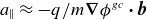 $a_\parallel \approx -q/m \boldsymbol{\nabla }\phi ^{gc} \boldsymbol{\cdot }\boldsymbol{b}$
.
$a_\parallel \approx -q/m \boldsymbol{\nabla }\phi ^{gc} \boldsymbol{\cdot }\boldsymbol{b}$
.
The turbulent potential
 $\phi$
is attributed to ion temperature gradient (ITG)\trapped electron mode (TEM) turbulence, with electron temperature gradient (ETG) contributions neglected. Gyroaveraging introduces finite-Larmor-radius corrections,
$\phi$
is attributed to ion temperature gradient (ITG)\trapped electron mode (TEM) turbulence, with electron temperature gradient (ETG) contributions neglected. Gyroaveraging introduces finite-Larmor-radius corrections,
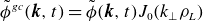 $\tilde {\phi }^{gc}(\boldsymbol{k},t) = \tilde {\phi }(\boldsymbol{k},t)J_0(k_\perp \rho _L)$
(Horton Reference Horton1999).
$\tilde {\phi }^{gc}(\boldsymbol{k},t) = \tilde {\phi }(\boldsymbol{k},t)J_0(k_\perp \rho _L)$
(Horton Reference Horton1999).
In the saturated regime, the turbulent potential
 $\phi (\boldsymbol{x},t)$
is modelled as a stationary, homogeneous, Gaussian random field with zero mean (Balescu Reference Balescu2005). Its statistical properties are fully determined by the two-point correlation function
$\phi (\boldsymbol{x},t)$
is modelled as a stationary, homogeneous, Gaussian random field with zero mean (Balescu Reference Balescu2005). Its statistical properties are fully determined by the two-point correlation function
 \begin{align} E(\boldsymbol{x},t|\boldsymbol{x}^\prime ,t^\prime )=\langle \phi (\boldsymbol{x},t)\phi (\boldsymbol{x}^\prime ,t^\prime )\rangle \equiv E(\boldsymbol{x}-\boldsymbol{x}^\prime ,|t-t^\prime |), \end{align}
or, equivalently, by the turbulence spectrum
 $S(\boldsymbol{k},\omega )$
(Palade & Vlad Reference Palade and Vlad2021).
$S(\boldsymbol{k},\omega )$
(Palade & Vlad Reference Palade and Vlad2021).
The transport coefficients are expressed in terms of gyrocentre trajectories
 $\boldsymbol{X}(t|x)$
evolving under equations (2.1)–(2.2) as
$\boldsymbol{X}(t|x)$
evolving under equations (2.1)–(2.2) as
 \begin{eqnarray} D(t|x) &\,=\,& \frac {1}{2}\frac{\text{d}}{\text{d}t} (\{\langle \boldsymbol{X}(t|x)^2\rangle \}-\{\langle \boldsymbol{X}(t|x)\rangle \}^2 ), \end{eqnarray}
 \begin{eqnarray} V(t|x) &\,=\,& \frac{\text{d}}{\text{d}t}\{\langle \boldsymbol{X}(t|x)\rangle \}, \end{eqnarray}
where
 $\boldsymbol{X}(t|x)$
denotes trajectories initialised at radial position
$\boldsymbol{X}(t|x)$
denotes trajectories initialised at radial position
 $x$
at
$x$
at
 $t=0$
, with all other phase-space coordinates sampled according to the equilibrium distribution. The coefficient
$t=0$
, with all other phase-space coordinates sampled according to the equilibrium distribution. The coefficient
 $D(t|x)$
thus provides a local estimate of radial diffusion. Here,
$D(t|x)$
thus provides a local estimate of radial diffusion. Here,
 $\langle \boldsymbol{\cdot }\rangle$
denotes ensemble averaging over turbulence realisations, while
$\langle \boldsymbol{\cdot }\rangle$
denotes ensemble averaging over turbulence realisations, while
 $\{\boldsymbol{\cdot }\}$
represents averaging over the remaining phase-space coordinates at fixed
$\{\boldsymbol{\cdot }\}$
represents averaging over the remaining phase-space coordinates at fixed
 $x$
, including the flux-surface average.
$x$
, including the flux-surface average.
2.2. The numerical code T3ST
The code T3ST (Turbulent Transport in Tokamaks via Stochastic Trajectories) Palade & Pomârjanschi (Reference Palade and Pomârjanschi2025) is a numerical framework for computing charged-particle gyrocentre trajectories in axisymmetric tokamak geometry with prescribed electrostatic turbulence, directly implementing the transport formalism previously described.
T3ST evolves an ensemble of
 $N_p$
independent test particles, each in a distinct realisation of the turbulent field. In this work, particles are initialised with a Maxwell–Boltzmann velocity distribution and are uniformly distributed in the
$N_p$
independent test particles, each in a distinct realisation of the turbulent field. In this work, particles are initialised with a Maxwell–Boltzmann velocity distribution and are uniformly distributed in the
 $(\theta ,\varphi )$
directions on a magnetic flux tube at fixed radius
$(\theta ,\varphi )$
directions on a magnetic flux tube at fixed radius
 $r=r_0$
.
$r=r_0$
.
In each field realisation, the synthetic turbulent potential is built with the aid of
 $N_c$
pairs of random wavenumbers and frequencies,
$N_c$
pairs of random wavenumbers and frequencies,
 $\{\boldsymbol{k}_i, \omega _i\}_{i,\in 1,N_c}$
, sampled from a probability distribution function (p.d.f.) defined by the normalised turbulence spectrum
$\{\boldsymbol{k}_i, \omega _i\}_{i,\in 1,N_c}$
, sampled from a probability distribution function (p.d.f.) defined by the normalised turbulence spectrum
 $S(\boldsymbol{k}, \omega )$
. The chaotic nature of fluctuations is also controlled by random phases
$S(\boldsymbol{k}, \omega )$
. The chaotic nature of fluctuations is also controlled by random phases
 $\alpha _i \in [0, 2\pi )$
that are assigned to each mode. The resulting potential (evaluated at the gyrocentre) is computed numerically as
$\alpha _i \in [0, 2\pi )$
that are assigned to each mode. The resulting potential (evaluated at the gyrocentre) is computed numerically as
 \begin{eqnarray} \phi _1^{gc}(\boldsymbol{X}, t) = \sqrt {\frac {2}{N_c}} \sum _{i=1}^{N_c} J_0(k_i^\perp \rho _L) \sin \left (\boldsymbol{k}_i \boldsymbol{\cdot }\boldsymbol{X} - \omega _i t + \alpha _i\right )\!, \end{eqnarray}
where the factor
 $\sqrt {2/N_c}$
ensures normalisation,
$\sqrt {2/N_c}$
ensures normalisation,
 $J_0(k_i^\perp \rho _L)$
accounts for finite Larmor radius (FLR) effects due to gyroaveraging and
$J_0(k_i^\perp \rho _L)$
accounts for finite Larmor radius (FLR) effects due to gyroaveraging and
 $k_i^\perp$
is the perpendicular component of
$k_i^\perp$
is the perpendicular component of
 $\boldsymbol{k}_i$
with respect to the local magnetic field. For further technical details, see Palade & Vlad (Reference Palade and Vlad2021), Iorga (Reference Iorga2023) and Palade & Pomârjanschi (Reference Palade and Pomârjanschi2025).
$\boldsymbol{k}_i$
with respect to the local magnetic field. For further technical details, see Palade & Vlad (Reference Palade and Vlad2021), Iorga (Reference Iorga2023) and Palade & Pomârjanschi (Reference Palade and Pomârjanschi2025).
To remain consistent with gyrokinetic conventions, field-aligned coordinates
 $(x, y, z)$
are used in the generation of turbulent fields (Beer, Cowley & Hammett Reference Beer, Cowley and Hammett1995), defined as
$(x, y, z)$
are used in the generation of turbulent fields (Beer, Cowley & Hammett Reference Beer, Cowley and Hammett1995), defined as
 \begin{equation} x = C_x \rho (\psi ) \approx r, \qquad y = C_y (\varphi - \bar {q} \chi ), \qquad z = C_z \chi , \end{equation}
where
 $C_x = a$
is the tokamak’s minor radius,
$C_x = a$
is the tokamak’s minor radius,
 $C_y = r_0 / \bar {q}(r_0)$
is a normalisation based on a reference radius
$C_y = r_0 / \bar {q}(r_0)$
is a normalisation based on a reference radius
 $r_0$
,
$r_0$
,
 $C_z = 1$
and
$C_z = 1$
and
 $\rho (\psi ) \equiv \rho _t = \sqrt {\varPhi _t(\psi )/\varPhi _t(\psi _{edge})}$
is the normalised effective radius, approximated by
$\rho (\psi ) \equiv \rho _t = \sqrt {\varPhi _t(\psi )/\varPhi _t(\psi _{edge})}$
is the normalised effective radius, approximated by
 $\rho _t \approx r/a$
in circular geometries. Here,
$\rho _t \approx r/a$
in circular geometries. Here,
 $\varPhi _t(\psi )$
is the toroidal magnetic flux
$\varPhi _t(\psi )$
is the toroidal magnetic flux
 $\varPhi _t(\psi ) = \int _{\psi _{axis}}^\psi \boldsymbol{B}\boldsymbol{\cdot }\boldsymbol{e}_\varphi\,\text{d} S(\psi ^\prime )$
measuring the flux enclosed between the axis and the surface labelled by
$\varPhi _t(\psi ) = \int _{\psi _{axis}}^\psi \boldsymbol{B}\boldsymbol{\cdot }\boldsymbol{e}_\varphi\,\text{d} S(\psi ^\prime )$
measuring the flux enclosed between the axis and the surface labelled by
 $\psi$
.
$\psi$
.
The turbulence spectrum
 $S(\boldsymbol{k}, \omega )$
used in this study captures key features of ITG-driven turbulence. It is constructed from analytical forms derived from saturation arguments and growth-rate-based heuristics (Staebler et al. Reference Staebler, Candy, Howard and Holland2016; Dudding et al. Reference Dudding, Casson, Dickinson, Patel, Roach, Belli and Staebler2022):
$S(\boldsymbol{k}, \omega )$
used in this study captures key features of ITG-driven turbulence. It is constructed from analytical forms derived from saturation arguments and growth-rate-based heuristics (Staebler et al. Reference Staebler, Candy, Howard and Holland2016; Dudding et al. Reference Dudding, Casson, Dickinson, Patel, Roach, Belli and Staebler2022):
 \begin{eqnarray} S(\boldsymbol{k}, \omega ) &=& A_\phi ^2 \frac {\tau _c \lambda _x \lambda _y \lambda _z}{(2\pi )^{5/2}} \frac {e^{-{k_x^2 \lambda _x^2 + k_z^2 \lambda _z^2}/{2}}}{1 + \tau _c^2 \omega ^2} \frac {k_y}{k_0} \times \big( e^{-{(k_y - k_0)^2 \lambda _y^2}/{2}} - e^{-{(k_y + k_0)^2 \lambda _y^2}/{2}} \big), \end{eqnarray}
where
 $\lambda _x$
,
$\lambda _x$
,
 $\lambda _y$
and
$\lambda _y$
and
 $\lambda _z$
are the spatial correlation lengths along the field-aligned directions
$\lambda _z$
are the spatial correlation lengths along the field-aligned directions
 $(x, y, z)$
,
$(x, y, z)$
,
 $k_0$
sets the characteristic scale of the most unstable mode (influenced jointly with
$k_0$
sets the characteristic scale of the most unstable mode (influenced jointly with
 $\lambda _y$
),
$\lambda _y$
),
 $\tau _c$
is the correlation time, representing the departure of actual mode frequencies from linear predictions due to nonlinear interactions, and
$\tau _c$
is the correlation time, representing the departure of actual mode frequencies from linear predictions due to nonlinear interactions, and
 $A_\phi$
characterises the turbulence amplitude.
$A_\phi$
characterises the turbulence amplitude.
2.3. Set-up of numerical simulations
While T3ST solves equations of motion that require many physical parameters, we restrict here to the famous scenario called the ‘Cyclone Base Case’ (CBC) that corresponds to a typical DIII-D discharge (Dimits et al. Reference Dimits, Cohen, Mattor, Nevins, Shumaker, Parker and Kim2000a
; Falchetto et al. Reference Falchetto2008). The values of the relevant parameters are
 $T_i=T_e=0.5\,\text{keV}, n_0=10^{19}\,\text{m}^{-3}, B_0 = 1.9T, R_0=1.71\,\text{m}, R_0/L_{T_i} =6.9, R_0/L_n=2.2, a= 0.625\,\text{m}, c_1 = 0.85, c_2 = 0, c_3 = 2.2, r_0 = a/2$
. Note that, in the case of
$T_i=T_e=0.5\,\text{keV}, n_0=10^{19}\,\text{m}^{-3}, B_0 = 1.9T, R_0=1.71\,\text{m}, R_0/L_{T_i} =6.9, R_0/L_n=2.2, a= 0.625\,\text{m}, c_1 = 0.85, c_2 = 0, c_3 = 2.2, r_0 = a/2$
. Note that, in the case of
 $H$
ions,
$H$
ions,
 $\rho _i/a=\rho ^\star \approx 1/519$
and the values for the safety factor
$\rho _i/a=\rho ^\star \approx 1/519$
and the values for the safety factor
 $q(r)=c_1+c_3(r/a)^2$
and magnetic shear
$q(r)=c_1+c_3(r/a)^2$
and magnetic shear
 $\hat {s}=\text{d}\ln \bar {q}/\text{d}\ln r$
are
$\hat {s}=\text{d}\ln \bar {q}/\text{d}\ln r$
are
 $\bar {q}(r_0) = 1.4, \hat {s} = 0.78$
. Gyrokinetic simulations (Lin & Hahm Reference Lin and Hahm2004) of this scenario have shown that the ITG turbulence develops from the dominant instability and has approximately constant phase velocity
$\bar {q}(r_0) = 1.4, \hat {s} = 0.78$
. Gyrokinetic simulations (Lin & Hahm Reference Lin and Hahm2004) of this scenario have shown that the ITG turbulence develops from the dominant instability and has approximately constant phase velocity
 $v_{ph}\approx V_\star \approx v_{th}\rho _i/L_n$
, i.e.
$v_{ph}\approx V_\star \approx v_{th}\rho _i/L_n$
, i.e.
 $\omega _{\boldsymbol{k}} \approx v_{ph}k_\theta$
. Regarding the growing rates
$\omega _{\boldsymbol{k}} \approx v_{ph}k_\theta$
. Regarding the growing rates
 $\gamma$
, they encompass the interval
$\gamma$
, they encompass the interval
 $[0,0.7]\rho _i^{-1}$
, with a maximum at
$[0,0.7]\rho _i^{-1}$
, with a maximum at
 $k_\theta \rho _i\approx 0.3$
. The turbulent amplitude at mid-radius in the saturated regime is
$k_\theta \rho _i\approx 0.3$
. The turbulent amplitude at mid-radius in the saturated regime is
 $\varPhi = eA_\phi /T_i\approx 1.1\,\%$
with a radial correlation length of
$\varPhi = eA_\phi /T_i\approx 1.1\,\%$
with a radial correlation length of
 $\lambda _r \approx 7\rho _i$
and a peaked spectrum in the poloidal wavenumber at
$\lambda _r \approx 7\rho _i$
and a peaked spectrum in the poloidal wavenumber at
 $k_\theta \rho _i\approx 0.15$
. Finally, the electrostatic potential is time-correlated (Lin & Hahm Reference Lin and Hahm2004)
$k_\theta \rho _i\approx 0.15$
. Finally, the electrostatic potential is time-correlated (Lin & Hahm Reference Lin and Hahm2004)
 $\langle \phi _1(\boldsymbol{x},t)\phi _1(\boldsymbol{x},0)\rangle \propto \exp (-t/\tau _c)$
with
$\langle \phi _1(\boldsymbol{x},t)\phi _1(\boldsymbol{x},0)\rangle \propto \exp (-t/\tau _c)$
with
 $\tau _c\approx 1/\gamma \approx 3/\omega \approx 10\rho _i/v_{ph}$
. For T3ST, these parameters translate into scaled values as
$\tau _c\approx 1/\gamma \approx 3/\omega \approx 10\rho _i/v_{ph}$
. For T3ST, these parameters translate into scaled values as
 $A_i = 1, \varPhi =0.011,\lambda _x=7,\lambda _y=5,k_0=0.05,\tau _c = 4$
, while
$A_i = 1, \varPhi =0.011,\lambda _x=7,\lambda _y=5,k_0=0.05,\tau _c = 4$
, while
 $\lambda _z\to \infty$
is chosen (no ballooning or parallel fluctuations).
$\lambda _z\to \infty$
is chosen (no ballooning or parallel fluctuations).
The present simulations are performed for
 ${}^{1}_{1}\mathrm{H}$
ions of the bulk plasma, thus, Maxwell–Boltzmann distributed with the temperature
${}^{1}_{1}\mathrm{H}$
ions of the bulk plasma, thus, Maxwell–Boltzmann distributed with the temperature
 $T_i$
. Unless otherwise specified, most simulations use
$T_i$
. Unless otherwise specified, most simulations use
 $N_p=5\times 10^{5}$
test-particles, each field realisation being constructed with
$N_p=5\times 10^{5}$
test-particles, each field realisation being constructed with
 $N_c = 10^2$
Fourier modes (2.7). The dynamics is followed over
$N_c = 10^2$
Fourier modes (2.7). The dynamics is followed over
 $t_{max}=60 R_0/v_{th}$
with a time-step of
$t_{max}=60 R_0/v_{th}$
with a time-step of
 $\Delta t = t_{max}/N_t, N_t=1500$
.
$\Delta t = t_{max}/N_t, N_t=1500$
.
For brevity, in § 3, whenever transport coefficients are discussed, they are evaluated at
 $x\equiv r=r_0$
and are denoted as
$x\equiv r=r_0$
and are denoted as
 $V(t)\equiv V(t|r_0), D(t)\equiv D(t|r_0)$
.
$V(t)\equiv V(t|r_0), D(t)\equiv D(t|r_0)$
.
3. Results
3.1. The dynamical scenario
Before answering questions about the Lagrangian features of turbulent transport, it is important to have a qualitative view on the nature of particle dynamics driven by ITG turbulence.
Evolution of test-particle positions in the
 $(R, Z)$
poloidal plane. Red markers show initial positions (
$(R, Z)$
poloidal plane. Red markers show initial positions (
 $t = 0$
) and blue markers show final positions (
$t = 0$
) and blue markers show final positions (
 $t = t_{max}$
).
$t = t_{max}$
).

The numerical simulations of T3ST assume, as initial distribution of particles, Maxwell–Boltzmann statistics in the energy-pitch-angle space and uniform distribution over a thin flux tube defined by
 $r = r_0 = a/2$
in the physical space (a circle in poloidal projection). This corresponds to a local Maxwellian (Vernay et al. Reference Vernay, Brunner, Villard, McMillan, Jolliet, Tran, Bottino and Graves2010), which is not an equilibrium distribution – unlike the canonical Maxwellian (Angelino et al. Reference Angelino, Bottino, Hatzky, Jolliet, Sauter, Tran and Villard2006; Garbet et al. Reference Garbet, Dif-Pradalier, Nguyen, Sarazin, Grandgirard and Ghendrih2009; Vernay et al. Reference Vernay, Brunner, Villard, McMillan, Jolliet, Tran, Bottino and Graves2010).
$r = r_0 = a/2$
in the physical space (a circle in poloidal projection). This corresponds to a local Maxwellian (Vernay et al. Reference Vernay, Brunner, Villard, McMillan, Jolliet, Tran, Bottino and Graves2010), which is not an equilibrium distribution – unlike the canonical Maxwellian (Angelino et al. Reference Angelino, Bottino, Hatzky, Jolliet, Sauter, Tran and Villard2006; Garbet et al. Reference Garbet, Dif-Pradalier, Nguyen, Sarazin, Grandgirard and Ghendrih2009; Vernay et al. Reference Vernay, Brunner, Villard, McMillan, Jolliet, Tran, Bottino and Graves2010).
Consequently, even if particles are allowed to move solely under the influence of magnetic drifts (with no turbulence) the distribution function will evolve manifesting finite Larmor radius (FLR) effects. However, the quiescent particle trajectories are periodic orbits (banana or passing) which means they are effectively confined. One expects the system to reach, eventually, a steady-state with no radial transport.
This scenario should be broken once turbulence is introduced since the low-
 $k$
drift-type ITG imparts – mainly via the
$k$
drift-type ITG imparts – mainly via the
 $\boldsymbol{v}_{E \times B}$
drift – correlated and continuous, but essentially random, kicks to particles. This should result in a non-equilibrium state with levels of transport that, hopefully, saturate asymptotically to finite values.
$\boldsymbol{v}_{E \times B}$
drift – correlated and continuous, but essentially random, kicks to particles. This should result in a non-equilibrium state with levels of transport that, hopefully, saturate asymptotically to finite values.
Numerical T3ST simulations are performed with or without turbulence. Figures 1(a) and 1(b) show, in the poloidal plane, the initial (red) and final (
 $t = t_{{max}}$
, blue) particle distributions for the purely quiescent (panel a) and the turbulent cases (panel b). In the quiescent case (figure 1
a), FLR effects are evident: gyrocentres do not remain on the initial flux surface, but spread along their orbits, producing a finite radial width – slightly broader on the low-field side. When turbulence is present (figure 1
b), particles undergo significant radial transport, effectively erasing the quiescent signature.
$t = t_{{max}}$
, blue) particle distributions for the purely quiescent (panel a) and the turbulent cases (panel b). In the quiescent case (figure 1
a), FLR effects are evident: gyrocentres do not remain on the initial flux surface, but spread along their orbits, producing a finite radial width – slightly broader on the low-field side. When turbulence is present (figure 1
b), particles undergo significant radial transport, effectively erasing the quiescent signature.
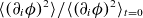
The expectation that quiescent motion leads asymptotically to confined equilibrium states with vanishing transport, while turbulence drives the system to non-equilibrium states with finite saturated transport is confirmed in figures 2(a) and 2(b). These plots show the time-dependent transport coefficients: diffusion
 $D(t)$
(panel a) and convection
$D(t)$
(panel a) and convection
 $V(t)$
(panel b). After a short transient period (
$V(t)$
(panel b). After a short transient period (
 $t \sim 20 R_0 / v_{th}$
), quiescent transport vanishes, while turbulent transport saturates to finite values. Notably, the convective term
$t \sim 20 R_0 / v_{th}$
), quiescent transport vanishes, while turbulent transport saturates to finite values. Notably, the convective term
 $V(t)$
is more susceptible to numerical fluctuations, despite both quantities being extracted from the same simulations. This peculiarity is explained in a recent work (Palade & Pomarjanschi Reference Palade and Pomarjanschi2026).
$V(t)$
is more susceptible to numerical fluctuations, despite both quantities being extracted from the same simulations. This peculiarity is explained in a recent work (Palade & Pomarjanschi Reference Palade and Pomarjanschi2026).
Time evolution of radial transport coefficients. In both panels, blue lines represent quiescent dynamics (no turbulence) and red lines represent turbulent dynamics. Diffusion saturates under turbulence, while it vanishes in the quiescent case.

Asymptotic (
 $t=t_{max}$
) distributions of radial particle positions in the (a) absence or the (b) presence of turbulence.
$t=t_{max}$
) distributions of radial particle positions in the (a) absence or the (b) presence of turbulence.

The diffusive character of turbulent transport is further evidenced by the radial particle distributions in figure 3(b), which approximates a Gaussian profile. In contrast, the quiescent case (figure 3
a) shows a narrower, symmetric distribution. These profiles can be understood by analysing also the distributions of Lagrangian radial velocities which can be seen in figures 4(a) and 4(b) at initial (
 $t = t_0$
, blue) and final (
$t = t_0$
, blue) and final (
 $t = t_{{max}}$
, red) times for the quiescent and turbulent cases, respectively. The nature of the profiles for velocities matches the profiles of radial tracers with or without turbulence. The reason for Gaussianity can be understood taking into account that turbulent drifts are, essentially, a sum of many random contributions (see (2.7) and the central limit theorem). Conversely, the long tails in the quiescent case are attributed to the relatively simple dependence of magnetic drifts on a limited number of variables. A simple estimate shows that the radial magnetic drift velocity is
$t = t_{{max}}$
, red) times for the quiescent and turbulent cases, respectively. The nature of the profiles for velocities matches the profiles of radial tracers with or without turbulence. The reason for Gaussianity can be understood taking into account that turbulent drifts are, essentially, a sum of many random contributions (see (2.7) and the central limit theorem). Conversely, the long tails in the quiescent case are attributed to the relatively simple dependence of magnetic drifts on a limited number of variables. A simple estimate shows that the radial magnetic drift velocity is
 \begin{align} V_r^{\text{neo}} &\approx -\frac {m\big(v_\parallel ^2 + v_\perp ^2 / 2\big)}{q B^3} (\boldsymbol{\nabla }B \times \boldsymbol{B}) \boldsymbol{\cdot }\boldsymbol{e}_r \nonumber \\[4pt] &\approx -\frac {(1 + \lambda ^2)E}{q B_0 R_0} \sin \theta = -\frac {v_{th}\rho _i}{R_0}(1 + \lambda ^2)\tilde {E} \sin \theta . \end{align}
Given that initially
 $\theta \in [0, 2\pi )$
,
$\theta \in [0, 2\pi )$
,
 $\lambda \in [-1, 1]$
and
$\lambda \in [-1, 1]$
and
 $P(\tilde {E}) \sim \sqrt {\tilde {E}} \exp (-\tilde {E})$
, the resulting distribution can be approximated numerically as
$P(\tilde {E}) \sim \sqrt {\tilde {E}} \exp (-\tilde {E})$
, the resulting distribution can be approximated numerically as
 $P[V_r^{\text{neo}}, t=0]\approx \exp (-0.9 |V_r|R_0/(v_{th}\rho _i))$
. This is in good accordance with the numerical data from figure 4(a).
$P[V_r^{\text{neo}}, t=0]\approx \exp (-0.9 |V_r|R_0/(v_{th}\rho _i))$
. This is in good accordance with the numerical data from figure 4(a).
What is remarkable is the fact that the velocity distributions seem to be extremely robust across dynamics with initial and asymptotic distributions matching almost perfectly (the overlapping of red and blue histograms results in a magenta hue, illustrating their near identity). This is a necessary condition for Lagrangian stationarity.
Radial Lagrangian velocity distributions at initial (blue) and final (red) simulation times.

3.2. The nature of the radial pinch
Figure 2(b) shows the effective running velocity coefficient
 $V(t)$
, defined as the time derivative of the average radial position of the particles. Since this quantity is not constant over time – but instead exhibits a transient growth phase before reaching a stationary value – this implies that Lagrangian stationarity is invalid. However, is this not in direct contradiction with the apparent identical distributions of initial and final radial velocities shown in figure 4(b)? The answer is that a small displacement of
$V(t)$
, defined as the time derivative of the average radial position of the particles. Since this quantity is not constant over time – but instead exhibits a transient growth phase before reaching a stationary value – this implies that Lagrangian stationarity is invalid. However, is this not in direct contradiction with the apparent identical distributions of initial and final radial velocities shown in figure 4(b)? The answer is that a small displacement of
 $V(t\to t_{max})\approx 2\,\mathrm{m\,s}^{-1}$
between distribution profiles in figure 4(b) is below the resolution of the figure, given that the mean square displacement (MSD) of velocities is
$V(t\to t_{max})\approx 2\,\mathrm{m\,s}^{-1}$
between distribution profiles in figure 4(b) is below the resolution of the figure, given that the mean square displacement (MSD) of velocities is
 $\sim\!1\,\mathrm{km\,s}^{-1}$
, that is, three orders of magnitude higher. Note that this also explains the noisy character of
$\sim\!1\,\mathrm{km\,s}^{-1}$
, that is, three orders of magnitude higher. Note that this also explains the noisy character of
 $V(t)$
.
$V(t)$
.
Effective velocity
 $V(t)$
(red, large fluctuations) compared with the normalised diffusion coefficient
$V(t)$
(red, large fluctuations) compared with the normalised diffusion coefficient
 $2D(t)/R$
(blue, smoother behaviour).
$2D(t)/R$
(blue, smoother behaviour).

At early times, the radial pinch arises from both quiescent and turbulent effects, given that both cases exhibit a similar growing phase. The asymptotic value, however, is driven solely by turbulence, since the quiescent case leads to
 $V(t)\to 0$
as
$V(t)\to 0$
as
 $t\to t_{max}$
. However, what is the mechanisms behind the existence of this effective pinch? Currently, there are several pinch mechanisms identified in the literature that rely on the existence of thermal, rotational (Camenen et al. Reference Camenen, Peeters, Angioni, Casson, Hornsby, Snodin and Strintzi2009), magnetic field inhomogeneities (Isichenko, Gruzinov & Diamond Reference Isichenko, Gruzinov and Diamond1995; Naulin, Nycander & Rasmussen Reference Naulin, Nycander and Rasmussen1998; Vlad, Spineanu & Benkadda Reference Vlad, Spineanu and Benkadda2006) or polarisation drifts (Palade Reference Palade2023). Since the present work does not include temperature gradients, toroidal rotation or polarisation drift effects, all these are excluded. It remains possible that the pinch is a turbulence equipartition pinch (TEP) (Isichenko et al. Reference Isichenko, Gruzinov and Diamond1995; Naulin et al. Reference Naulin, Nycander and Rasmussen1998; Vlad et al. Reference Vlad, Spineanu and Benkadda2006) which relies on the inhomogeneity of the magnetic field and on the compressibility of the
$t\to t_{max}$
. However, what is the mechanisms behind the existence of this effective pinch? Currently, there are several pinch mechanisms identified in the literature that rely on the existence of thermal, rotational (Camenen et al. Reference Camenen, Peeters, Angioni, Casson, Hornsby, Snodin and Strintzi2009), magnetic field inhomogeneities (Isichenko, Gruzinov & Diamond Reference Isichenko, Gruzinov and Diamond1995; Naulin, Nycander & Rasmussen Reference Naulin, Nycander and Rasmussen1998; Vlad, Spineanu & Benkadda Reference Vlad, Spineanu and Benkadda2006) or polarisation drifts (Palade Reference Palade2023). Since the present work does not include temperature gradients, toroidal rotation or polarisation drift effects, all these are excluded. It remains possible that the pinch is a turbulence equipartition pinch (TEP) (Isichenko et al. Reference Isichenko, Gruzinov and Diamond1995; Naulin et al. Reference Naulin, Nycander and Rasmussen1998; Vlad et al. Reference Vlad, Spineanu and Benkadda2006) which relies on the inhomogeneity of the magnetic field and on the compressibility of the
 $\boldsymbol{v}_{E\times B}$
drift.
$\boldsymbol{v}_{E\times B}$
drift.
The nature of this effect can be emphasised with a simple perturbative calculus, using the linearisation
 $B(\boldsymbol{x})^{-1}\approx B(\boldsymbol{0})^{-1} - B(\boldsymbol{0})^{-2} \boldsymbol{x}\boldsymbol{\nabla }B(\boldsymbol{0})$
:
$B(\boldsymbol{x})^{-1}\approx B(\boldsymbol{0})^{-1} - B(\boldsymbol{0})^{-2} \boldsymbol{x}\boldsymbol{\nabla }B(\boldsymbol{0})$
:
 \begin{align} \boldsymbol{v}_{E\times B}(\boldsymbol{X}(t),t) &= \frac {\boldsymbol{b} \times \boldsymbol{\nabla }\phi (\boldsymbol{X}(t),t)}{B} \nonumber \\[5pt] &\approx \frac {\boldsymbol{b} \times \boldsymbol{\nabla }\phi (\boldsymbol{X}(t),t)}{B(\boldsymbol{0})} \left (1 - \boldsymbol{X}(t) \boldsymbol{\cdot }\boldsymbol{\nabla }\ln B(\boldsymbol{0}) \right )\!. \end{align}
Taking the ensemble average and considering an homogeneous distribution of positions
 $\boldsymbol{X}(t)$
that are driven mainly by the
$\boldsymbol{X}(t)$
that are driven mainly by the
 $E\times B$
drift, it yields
$E\times B$
drift, it yields
 \begin{align} V(t)&=\left \langle \frac {\boldsymbol{b} \times \boldsymbol{\nabla }\phi (\boldsymbol{X}(t),t)}{B(\boldsymbol{0})} \int _0^t \text{d}\tau \frac {\boldsymbol{b} \times \boldsymbol{\nabla }\phi (\boldsymbol{X}(\tau ),\tau )}{B(\boldsymbol{0})} \boldsymbol{\cdot }\boldsymbol{\nabla }\ln B(\boldsymbol{0}) \right \rangle \nonumber \\[5pt] & = \int _0^t \text{d}\tau \left \langle \frac {\boldsymbol{b} \times \boldsymbol{\nabla }\phi (\boldsymbol{X}(t),t)}{B(\boldsymbol{0})} \frac {\boldsymbol{b} \times \boldsymbol{\nabla }\phi (\boldsymbol{X}(\tau ),\tau )}{B(\boldsymbol{0})} \right \rangle \boldsymbol{\cdot }\boldsymbol{\nabla }\ln B(\boldsymbol{0}) \nonumber \\[5pt] &\approx \int _0^t \text{d}\tau \left \langle V_r(t)V_r(\tau )\right \rangle \boldsymbol{\cdot }\partial _r \ln B(\boldsymbol{0}) \propto \frac {2D(t)}{R_0}. \end{align}
In the final step, we have identified the expression of diffusion as time-integral of the velocity auto-correlation. It turns out that the numerical results are very much in line with this approximate dependency (see figure 5); thus, the TEP is confirmed.
3.3. Lagrangian stationarity
Previously, results shown in figures 4(a) and 4(b) suggested that the distributions
 $P[V_r]$
of radial Lagrangian velocities of particles are almost identical between the starting point of the simulation
$P[V_r]$
of radial Lagrangian velocities of particles are almost identical between the starting point of the simulation
 $t=0$
and the final time
$t=0$
and the final time
 $t=t_{max}=60R_0/v_{th}$
. A closer inspection into figure 5 has revealed that this is not entirely true: particles do experience an average Lagrangian velocity
$t=t_{max}=60R_0/v_{th}$
. A closer inspection into figure 5 has revealed that this is not entirely true: particles do experience an average Lagrangian velocity
 $V(t)$
which is of TEP nature and results from the inhomogeneity of the magnetic field. It is not visible in the plot of distributions due to scale disparity:
$V(t)$
which is of TEP nature and results from the inhomogeneity of the magnetic field. It is not visible in the plot of distributions due to scale disparity:
 $V(t)=\langle V_r(t)\rangle \sim 1\,\mathrm{m\,s}^{-1}$
, while
$V(t)=\langle V_r(t)\rangle \sim 1\,\mathrm{m\,s}^{-1}$
, while
 $\sqrt {\langle V_r^2(t)\rangle }\sim 1\,\mathrm{km\,s}^{-1}$
. Thus, we conclude that stationarity is broken for the average of velocities, but is approximately valid in the asymptotic region.
$\sqrt {\langle V_r^2(t)\rangle }\sim 1\,\mathrm{km\,s}^{-1}$
. Thus, we conclude that stationarity is broken for the average of velocities, but is approximately valid in the asymptotic region.
Lagrangian auto-correlation
 $L(t,t^\prime )$
of radial velocity fields in the (a) quiescent and (b) turbulent cases.
$L(t,t^\prime )$
of radial velocity fields in the (a) quiescent and (b) turbulent cases.

Lagrangian auto-correlation
 $L(t_0,t_0+t)$
evaluated in the (a) quiescent and (b) turbulent cases for
$L(t_0,t_0+t)$
evaluated in the (a) quiescent and (b) turbulent cases for
 $t_0 = 0,5,10,15,20 R_0/v_{th}$
(red, blue, green, brown, black, respectively, lines). The curves are essentially indistinguishable.
$t_0 = 0,5,10,15,20 R_0/v_{th}$
(red, blue, green, brown, black, respectively, lines). The curves are essentially indistinguishable.

We look further to the Lagrangian velocity auto-correlation along the radial direction, defined, in this work’s notation, as
 \begin{eqnarray} L(t,t^\prime ) = \{\langle V_r(t)V_r(t^\prime )\rangle \}-\{\langle V_r(t)\rangle \}\{\langle V_r(t^\prime )\rangle \}. \end{eqnarray}
If the dynamics would be truly stationary, this quantity should be time-invariant, i.e.
 $L(t,t^\prime )\equiv L(|t-t^\prime |,0)$
. Figures 6(a) and 6(b) plot precisely
$L(t,t^\prime )\equiv L(|t-t^\prime |,0)$
. Figures 6(a) and 6(b) plot precisely
 $L$
for the quiescent and the turbulent case, respectively. It appears that, at least qualitatively, the graphs are in both cases symmetrical, implying stationarity. The matter can be explored further by investigating slices of
$L$
for the quiescent and the turbulent case, respectively. It appears that, at least qualitatively, the graphs are in both cases symmetrical, implying stationarity. The matter can be explored further by investigating slices of
 $L(t_0,t_0+t)$
in terms of the time-difference
$L(t_0,t_0+t)$
in terms of the time-difference
 $t$
. This is shown for many
$t$
. This is shown for many
 $t_0$
values in figures 7(a) and 7(b) (quiescent and turbulent case) and in figures 8(a) and 8(b) for only two values (
$t_0$
values in figures 7(a) and 7(b) (quiescent and turbulent case) and in figures 8(a) and 8(b) for only two values (
 $t_0 = 0$
– blue line and
$t_0 = 0$
– blue line and
 $t_0=30$
– red line). In all these figures, the lines are virtually indistinguishable, thus signalling almost perfect stationarity of the Lagrangian velocities across the super-ensemble.
$t_0=30$
– red line). In all these figures, the lines are virtually indistinguishable, thus signalling almost perfect stationarity of the Lagrangian velocities across the super-ensemble.
Lagrangian auto-correlation
 $L(t_0,t_0+t)$
evaluated in the (a) quiescent and (b) tur-bulent cases for
$L(t_0,t_0+t)$
evaluated in the (a) quiescent and (b) tur-bulent cases for
 $t_0 = 0,20 R_0/v_{th}$
(blue, red lines). The curves are hardly distinguishable.
$t_0 = 0,20 R_0/v_{th}$
(blue, red lines). The curves are hardly distinguishable.

We now go back to the local in time dynamics and ask wether the second-order cumulant of Lagrangian velocities is time-invariant. It so happens that this quantity is identical to the diagonal part of the correlation function, i.e.
 $\{\langle V^2(t)\rangle \} - \{\langle V(t)\rangle \}^2 = L(t,t)$
. The results are shown in figure 9, where small departures from stationarity, i.e.
$\{\langle V^2(t)\rangle \} - \{\langle V(t)\rangle \}^2 = L(t,t)$
. The results are shown in figure 9, where small departures from stationarity, i.e.
 ${\sim} 1\,\%$
, can be observed both for the quiescent (blue) and the turbulent (red) cases. While in the former case one observes only a transient growth followed by a saturation, the latter exhibits continuous linear growth. This again must be connected with the inhomogeneity of
${\sim} 1\,\%$
, can be observed both for the quiescent (blue) and the turbulent (red) cases. While in the former case one observes only a transient growth followed by a saturation, the latter exhibits continuous linear growth. This again must be connected with the inhomogeneity of
 $B$
and it suggests that the transport might not even be perfectly saturated (or local, for that matter).
$B$
and it suggests that the transport might not even be perfectly saturated (or local, for that matter).
Time evolution of the second moment of the distribution of velocities scaled to its initial value
 $\{\langle V^2(t)\rangle \} - \{\langle V(t)\rangle \}^2 = L(t,t)$
for the quiescent (blue) and the turbulent (red) cases.
$\{\langle V^2(t)\rangle \} - \{\langle V(t)\rangle \}^2 = L(t,t)$
for the quiescent (blue) and the turbulent (red) cases.

Thus, given the results from this section, one can conclude that the Lagrangian stationarity is approximately present, with small deviations that are, in general, quantifiable to
 ${\sim} 1\,\%$
.
${\sim} 1\,\%$
.
A more surprising aspect is that there is stationarity in the quiescent case. This cannot be attributed to the approximate homogeneity of the turbulence and it is in apparent striking conflict with the fact that magnetic drifts in (3.1) are starkly inhomogeneous. The only player in this picture that could drive Lagrangian stationarity are the particles, more precisely, their guiding-centre coordinates. Indeed, the initial phase-space distribution function used by T3ST, although it is one of non-equilibrium, evolves conserving the phase-space volume. Given how wide it is, it must be the reason behind Lagrangian homogeneity and ergodicity.
3.4. Statistics of field derivatives
The Lagrangian stationarity of the velocity statistics was proven to be approximately true, despite the inhomogeneous and compressible nature of the Eulerian drift field. A natural extension of this analysis is to investigate whether the Lagrangian statistics of the potential gradients, which directly generate the turbulent
 $\boldsymbol{E} \times \boldsymbol{B}$
drift, also exhibit stationary behaviour over time.
$\boldsymbol{E} \times \boldsymbol{B}$
drift, also exhibit stationary behaviour over time.
In the gyrokinetic approximation, the dominant turbulent contribution to particle motion arises from the electrostatic potential via the drift:
 \begin{equation} \boldsymbol{v}_{E \times B} = \frac {\boldsymbol{b} \times \boldsymbol{\nabla }\phi }{B}, \end{equation}
where
 $\phi$
is the fluctuating electrostatic potential evaluated at the gyrocentre. Therefore, the gradients
$\phi$
is the fluctuating electrostatic potential evaluated at the gyrocentre. Therefore, the gradients
 $\boldsymbol{\nabla }\phi$
– and in particular, their Lagrangian statistics – are key drivers of transport.
$\boldsymbol{\nabla }\phi$
– and in particular, their Lagrangian statistics – are key drivers of transport.
We compute the first- and second-order Lagrangian statistics of the field derivatives over time, namely
 \begin{equation} \left \langle \partial _i \phi (t) \right \rangle \quad \text{and} \quad \langle \left ( \partial _i \phi (t) \right )^2 \rangle , \quad i \in \{x, y\}, \end{equation}
where the spatial derivatives are evaluated along test-particle trajectories and averaged over the super-ensemble.
Figure 10(a) shows the time evolution of the average values
 $\left \langle \partial _x \phi \right \rangle$
and
$\left \langle \partial _x \phi \right \rangle$
and
 $ \langle \partial _y \phi \rangle$
, normalised by their respective standard deviations. Both quantities remain very close to zero throughout the simulation time, indicating that there is no net directional bias in the turbulent forcing fields along particle paths. This is consistent with the Eulerian property that the turbulent potential has zero mean and is symmetric in space.
$ \langle \partial _y \phi \rangle$
, normalised by their respective standard deviations. Both quantities remain very close to zero throughout the simulation time, indicating that there is no net directional bias in the turbulent forcing fields along particle paths. This is consistent with the Eulerian property that the turbulent potential has zero mean and is symmetric in space.
Time evolution of the Lagrangian average of (a) field derivatives
 $\{\langle \partial _x\phi (t)\rangle \},\{\langle \partial _y\phi (t)\rangle \}$
(red, blue) and (b) derivative amplitudes
$\{\langle \partial _x\phi (t)\rangle \},\{\langle \partial _y\phi (t)\rangle \}$
(red, blue) and (b) derivative amplitudes
 $\{\langle (\partial _x\phi (t))^2\rangle \},\{\langle (\partial _x\phi (t))^2\rangle \}$
(red, blue). (c) Distribution of poloidal derivatives
$\{\langle (\partial _x\phi (t))^2\rangle \},\{\langle (\partial _x\phi (t))^2\rangle \}$
(red, blue). (c) Distribution of poloidal derivatives
 $\partial _y\phi (t)$
at the initial (blue,
$\partial _y\phi (t)$
at the initial (blue,
 $t=t_0$
) and the final (red,
$t=t_0$
) and the final (red,
 $t=t_{max}$
) simulation times.
$t=t_{max}$
) simulation times.

Figure 10(b) presents the normalised second moments
 $\langle ( \partial _i \phi )^2 \rangle / \langle ( \partial _i \phi )^2 \rangle _{t=0}$
, which represent the average amplitude of the turbulent gradients as experienced along Lagrangian trajectories. These amplitudes remain stable over time, with only small fluctuations (below
$\langle ( \partial _i \phi )^2 \rangle / \langle ( \partial _i \phi )^2 \rangle _{t=0}$
, which represent the average amplitude of the turbulent gradients as experienced along Lagrangian trajectories. These amplitudes remain stable over time, with only small fluctuations (below
 $2\,\%$
) relative to their initial values. This indicates that the turbulence maintains its effective strength along the paths of particles and supports the earlier observation of approximate Lagrangian stationarity in drift velocities.
$2\,\%$
) relative to their initial values. This indicates that the turbulence maintains its effective strength along the paths of particles and supports the earlier observation of approximate Lagrangian stationarity in drift velocities.
Additionally, figure 10(c) compares the probability distributions
 $P[\partial _y \phi ]$
(
$P[\partial _y \phi ]$
(
 $\partial _y \phi$
is the main contribution to radial transport) at the initial and final simulation times. The distributions are nearly indistinguishable and closely approximate Gaussian profiles, consistent with the assumption of normally distributed fluctuations in
$\partial _y \phi$
is the main contribution to radial transport) at the initial and final simulation times. The distributions are nearly indistinguishable and closely approximate Gaussian profiles, consistent with the assumption of normally distributed fluctuations in
 $\phi$
. The invariance of these distributions over time provides further evidence for the ergodic and statistically stationary character of the turbulent forcing fields along gyrocentre trajectories.
$\phi$
. The invariance of these distributions over time provides further evidence for the ergodic and statistically stationary character of the turbulent forcing fields along gyrocentre trajectories.
Taken together, these results reinforce the conclusion that not only the Lagrangian velocities, but also the turbulent driving gradients remain approximately statistically stationary over time, despite the fact that the Eulerian fields themselves are inhomogeneous and compressible.
3.5. Time-symmetry
Lagrangian stationarity, in the general case, does not require nor does it imply time-reversibility/symmetry. The applicability of the Lagrangian method for the calculation of diffusion (
 $D_L(t)$
, see § 3.8), however, requires symmetry since the Lagrangian velocity auto-correlation must obey
$D_L(t)$
, see § 3.8), however, requires symmetry since the Lagrangian velocity auto-correlation must obey
 $L(t,t^\prime )= L(t-t^\prime ,0)=L(t^\prime -t,0)$
. For this reason, in this section, the time-symmetry of turbulent transport is investigated.
$L(t,t^\prime )= L(t-t^\prime ,0)=L(t^\prime -t,0)$
. For this reason, in this section, the time-symmetry of turbulent transport is investigated.
(a) Running diffusion and (b) velocity coefficients for quiescent (dashed lines) and turbulent (solid lines) dynamics, computed forward (red) and backward (blue) in time.

The time direction in the numerical integration of particle trajectories is simply inverted. We then compare transport quantities: diffusion (figure 11 a) and velocity (figure 11 b) coefficients, radial particle distributions (figure 12), and the Lagrangian velocity autocorrelation (figure 13).
Long-time (
 $t = t_{{max}}$
) distribution of particle radial positions for (a) quiescent and (b) turbulent dynamics, computed forward (red) and backward (blue) in time.
$t = t_{{max}}$
) distribution of particle radial positions for (a) quiescent and (b) turbulent dynamics, computed forward (red) and backward (blue) in time.

Figures 11(a) and 11(b) show that forward (red) and backward (blue) transport coefficients are nearly symmetric with respect to
 $t = 0$
, for both quiescent and turbulent dynamics. This symmetry, apart from small numerical fluctuations, indicates that the transport is effectively time-reversible.
$t = 0$
, for both quiescent and turbulent dynamics. This symmetry, apart from small numerical fluctuations, indicates that the transport is effectively time-reversible.
This conclusion is further supported by figures 12(a) and 12(b) that present the final distributions of radial particle positions. They are nearly identical in the forward and backward simulations, indicating an even stronger manifestation of time-symmetric dynamics. Finally, figure 13 shows that the Lagrangian velocity autocorrelation
 $L(t_0, t_0 + t)$
also exhibits the same symmetry between forward (dashed) and backward (solid) time evolutions.
$L(t_0, t_0 + t)$
also exhibits the same symmetry between forward (dashed) and backward (solid) time evolutions.
Lagrangian velocity autocorrelation
 $L(t_0, t_0 + t)$
for the turbulent case, evaluated at
$L(t_0, t_0 + t)$
for the turbulent case, evaluated at
 $t_0 = 0$
and
$t_0 = 0$
and
 $t_0 = 20 R_0 / v_{th}$
(blue and red lines), for forward (dashed) and backward (solid) dynamics.
$t_0 = 20 R_0 / v_{th}$
(blue and red lines), for forward (dashed) and backward (solid) dynamics.

These findings are consistent with the structure of the equations of motion (2.1)–(2.2). The magnetic drifts are time-independent, while the turbulent fields introduce time dependence through their mode frequencies
 $\omega = \omega _\star (\boldsymbol{k})+\Delta \omega$
. Part of this time dependence
$\omega = \omega _\star (\boldsymbol{k})+\Delta \omega$
. Part of this time dependence
 $\Delta \omega$
arises from nonlinear saturation processes, which contribute symmetrically in time and are governed by the decorrelation time
$\Delta \omega$
arises from nonlinear saturation processes, which contribute symmetrically in time and are governed by the decorrelation time
 $\tau _c$
. These components do not break time-reversibility. The dispersive part
$\tau _c$
. These components do not break time-reversibility. The dispersive part
 $\omega _\star (\boldsymbol{k})$
imposes a preferential direction in space and time for the drift of turbulent waves. However, the plasma equilibrium and particle distributions are space–time symmetrical relative to this special direction of drift, thus, inverting time switches the ITG into a TEM-like instability, but without affecting the radial transport.
$\omega _\star (\boldsymbol{k})$
imposes a preferential direction in space and time for the drift of turbulent waves. However, the plasma equilibrium and particle distributions are space–time symmetrical relative to this special direction of drift, thus, inverting time switches the ITG into a TEM-like instability, but without affecting the radial transport.
3.6. On the validity of the statistical approach
As detailed in § 1, the use of statistical ensembles to study turbulent transport can be motivated by the epistemic argument that turbulence is chaotic and its configuration cannot be precisely known. The rigorous argument is rather ontic and relies on ergodicity that arises from space-homogeneity, time-stationarity and incompressibility of the Eulerian velocity field
 $\boldsymbol{v}(\boldsymbol{x},t)$
. Given that these properties are not perfectly met by the gyrocentre drifts in tokamaks, we ask here wether a statistical ensemble of turbulent potentials
$\boldsymbol{v}(\boldsymbol{x},t)$
. Given that these properties are not perfectly met by the gyrocentre drifts in tokamaks, we ask here wether a statistical ensemble of turbulent potentials
 $\phi (\boldsymbol{x},t)$
is able to produce transport features similar to a single field realisation.
$\phi (\boldsymbol{x},t)$
is able to produce transport features similar to a single field realisation.
Running diffusion coefficient for the turbulent regime, evaluated for a single field realisation (red, solid line) and for a statistical ensemble of realisations (blue, dashed line).

Two numerical simulations are performed. In the first,
 $N_p$
particles evolve in a single turbulent field realisation (shared by all particles); in the second, each of the
$N_p$
particles evolve in a single turbulent field realisation (shared by all particles); in the second, each of the
 $N_p$
particles evolves in its own independent realisation of the turbulent field. The resulting diffusion coefficients for both cases are shown in figure 14. Minor differences
$N_p$
particles evolves in its own independent realisation of the turbulent field. The resulting diffusion coefficients for both cases are shown in figure 14. Minor differences
 ${\sim} 5\,\%$
can be observed across the entire time profile and stem from numerical fluctuations. It is interesting to note that the latter seem to have similar amplitudes in both cases. This suggests that the numerical noise is independent of the number of realisations.
${\sim} 5\,\%$
can be observed across the entire time profile and stem from numerical fluctuations. It is interesting to note that the latter seem to have similar amplitudes in both cases. This suggests that the numerical noise is independent of the number of realisations.
Thus, at least from the perspective of transport, modelling turbulence via an ensemble of random fields is equivalent to using a single realisation of a chaotic field.
3.7. The influence of initial distributions
Up to this point, all numerical results have indicated approximate Lagrangian stationarity of the turbulent dynamical processes, despite the Eulerian inhomogeneity of magnetic fields and
 $\boldsymbol{E}\times \boldsymbol{B}$
drifts. This behaviour was attributed to the space–time ergodicity of particle trajectories, which in practice is supported by the broad initial distribution of particles in phase space which induce ergodic mixing. This hypothesis will be tested in this and the next section.
$\boldsymbol{E}\times \boldsymbol{B}$
drifts. This behaviour was attributed to the space–time ergodicity of particle trajectories, which in practice is supported by the broad initial distribution of particles in phase space which induce ergodic mixing. This hypothesis will be tested in this and the next section.
Here, we focus specifically on the impact of initial conditions on transport – particularly on the computed diffusion coefficients. Beyond its relevance to Lagrangian stationarity, this topic is important for a fundamental reason: in deriving Fick-like transport laws,
 $\varGamma = V n -D\boldsymbol{\nabla }n$
, whether from Onsager symmetry relations or Green–Kubo relations, it is generally assumed that the distribution function is either an equilibrium or a statistical average.
$\varGamma = V n -D\boldsymbol{\nabla }n$
, whether from Onsager symmetry relations or Green–Kubo relations, it is generally assumed that the distribution function is either an equilibrium or a statistical average.
However, in T3ST, particles are typically initialised uniformly over a flux-tube with a Maxwell–Boltzmann velocity distribution. This does not represent an equilibrium distribution, nor does it reflect the dynamical statistical average. A more consistent approach would be to initialise particles in either a known equilibrium state (such as a canonical Maxwellian) or a steady-state – like the one reached asymptotically under pure magnetic motion. Unfortunately, both alternatives would require additional and non-trivial numerical procedures.
Comparison of running radial diffusion coefficients obtained under different initial conditions.

To explore the sensitivity of transport to initial phase-space distributions, we carry out several comparative numerical simulations which differ from the typical simulation described in § 2.3 through one of the following:
-
(i) initial pitch angles are fixed at
 $\lambda = 0.3$
;
$\lambda = 0.3$
; -
(ii) initial energies are fixed at
$E = T_i$
; -
(iii) particles are placed at a single radial point on the low-field side (LFS);
-
(iv) turbulence is later, at
$t = 35R_0/v_{th}$
, after the particles reach a quasi-steady quiescent state; -
(v) initial pitch angles and energies are concurrently set to
$\lambda =0.3, E=T_i$
; -
(vi) initial pitch angles are set to
$\lambda =0.3$
and particle placed at the low-field side (LFS); -
(vii) initial energies are set to
$E=T_i$
and particle placed at the LFS.


The first four scenarios constitute a mild degradation (restriction) of the initial filling of the phase space. Their associated radial diffusion coefficients are shown in figure 15(a). Perhaps surprisingly, aside from short-time transients, the resulting asymptotic diffusion coefficients are largely insensitive to the choice of initial conditions. The only notable deviation occurs when particles are initialised exclusively at the LFS line, which leads to a modest (
 ${\sim} 5\,\%$
) change in the long-time diffusion coefficient.
${\sim} 5\,\%$
) change in the long-time diffusion coefficient.
The most significant result shown in figure 15(a) is that the asymptotic diffusion coefficients are virtually identical regardless of whether turbulence is activated at
 $t=0$
(black) or later, at
$t=0$
(black) or later, at
 $t=35R_0/v_{th}$
(red). This indicates that initialising turbulence on a non-equilibrium particle distribution (the standard T3ST scenario) yields essentially the same asymptotic transport as starting from a near-equilibrium distribution. This is particularly valuable, as it justifies the use of the simpler and computationally cheaper red scenario.
$t=35R_0/v_{th}$
(red). This indicates that initialising turbulence on a non-equilibrium particle distribution (the standard T3ST scenario) yields essentially the same asymptotic transport as starting from a near-equilibrium distribution. This is particularly valuable, as it justifies the use of the simpler and computationally cheaper red scenario.
We proceed further to the last three cases which are a consistent degradation of the initial phase space occupied volume by the particles. The results are shown in figure 15(b). The time profiles of diffusions and their asymptotic values are somehow more dispersed, but they are still surprisingly close (
 ${\sim} 20\,\%$
). This tells us that even a modest initial filling of the phase space leads to similar transport as much more extended distributions (the standard case).
${\sim} 20\,\%$
). This tells us that even a modest initial filling of the phase space leads to similar transport as much more extended distributions (the standard case).
3.8. Two methods of computing diffusion
If the Lagrangian velocity auto-correlation function is indeed stationary – as approximately suggested in § 3.6 – i.e.
 $L(t, t^\prime ) \equiv L(|t - t^\prime |,0)$
, then the following definitions of the diffusion coefficient should be equivalent,
$L(t, t^\prime ) \equiv L(|t - t^\prime |,0)$
, then the following definitions of the diffusion coefficient should be equivalent,
 $D_d(t) = D_L(t)$
:
$D_d(t) = D_L(t)$
:
 \begin{eqnarray} D_d(t) &\,=\,& \frac {1}{2} \frac{\text{d}}{\text{d}t}\left \langle \delta x^2(t) \right \rangle, \end{eqnarray}
 \begin{eqnarray} D_L(t) &\,=\,& \int _0^t L(\tau ) \, \text{d}\tau . \end{eqnarray}
This equivalence is important for many theoretical and computational approaches. In particular, it underlies the decorrelation trajectory method (DTM) (Vlad et al. Reference Vlad, Spineanu, Misguich and Balescu1998), which has been widely applied in the study of turbulent transport in fluids (Vlad et al. Reference Vlad, Spineanu, Misguich and Balescu2001), tokamaks (Vlad et al. Reference Vlad, Spineanu, Misguich and Balescu2000; Palade, Vlad & Spineanu Reference Palade, Vlad and Spineanu2021; Vlad, Palade & Spineanu Reference Palade, Vlad and Spineanu2021) and astrophysical plasmas (Vlad Reference Vlad2018). An alternative view on the matter can be drawn from the fact that
 $D_L(t)$
is, in reality, a Green–Kubo relation which stems from the fluctuation–dissipation theorem (Kubo Reference Kubo1966). The latter requires ergodicity and time-translational invariance (Vainstein, Costa & Oliveira Reference Vainstein, Costa and Oliveira2006).
$D_L(t)$
is, in reality, a Green–Kubo relation which stems from the fluctuation–dissipation theorem (Kubo Reference Kubo1966). The latter requires ergodicity and time-translational invariance (Vainstein, Costa & Oliveira Reference Vainstein, Costa and Oliveira2006).
Running diffusion coefficients computed using the MSD-based method
 $D_d$
(red) and the Lagrangian correlation method
$D_d$
(red) and the Lagrangian correlation method
 $D_L$
(blue) for both the quiescent (dashed lines) and turbulent (solid lines) cases.
$D_L$
(blue) for both the quiescent (dashed lines) and turbulent (solid lines) cases.

We assess the validity of the equality
 $D_d(t) = D_L(t)$
by comparing numerical data. They are shown in figure 16, where the MSD-derived diffusion coefficient
$D_d(t) = D_L(t)$
by comparing numerical data. They are shown in figure 16, where the MSD-derived diffusion coefficient
 $D_d^{(X)}(t)$
is plotted in red and the correlation-based estimate
$D_d^{(X)}(t)$
is plotted in red and the correlation-based estimate
 $D_L^{(X)}(t)$
in blue for
$D_L^{(X)}(t)$
in blue for
 $X=$
neo (dashed lines) and
$X=$
neo (dashed lines) and
 $X=$
turb (filled lines). The agreement between the two methods is remarkably close, with only small
$X=$
turb (filled lines). The agreement between the two methods is remarkably close, with only small
 ${\sim} 1\,\%$
discrepancies. This suggests, once again, good but not perfect stationarity of the Lagrangian correlation function
${\sim} 1\,\%$
discrepancies. This suggests, once again, good but not perfect stationarity of the Lagrangian correlation function
 $L(t, t')$
.
$L(t, t')$
.
According to figure 16, the Lagrangian method of computing diffusion seems to provide a much smoother time-profile that saturates at the same asymptotic values as the differential method
 $D_d$
. This smoothness makes
$D_d$
. This smoothness makes
 $D_L$
an attractive alternative of computation with much less numerical noise to computing effort ratio. This is further supported by the histograms in figures 17(a) and 17(b) that show the distributions of saturated (
$D_L$
an attractive alternative of computation with much less numerical noise to computing effort ratio. This is further supported by the histograms in figures 17(a) and 17(b) that show the distributions of saturated (
 $t \gt 40$
) diffusion values obtained via
$t \gt 40$
) diffusion values obtained via
 $D_d$
and
$D_d$
and
 $D_L$
.
$D_L$
.
The explanation for this difference is two-fold. First, the numerical fluctuations in the velocity correlation function are smoothed through time integration in the Lagrangian method, whereas the MSD method amplifies noise due to time differentiation. Second, the uncertainty in MSD scales with the square of the noise amplitude,
 $\sim\!A_{\text{noise}}^2$
, because it involves squaring particle displacements. In contrast, the uncertainty in the autocorrelation function scales linearly,
$\sim\!A_{\text{noise}}^2$
, because it involves squaring particle displacements. In contrast, the uncertainty in the autocorrelation function scales linearly,
 $\sim\!A_{\text{noise}}$
. Thus, for finite particle ensembles, the Lagrangian method is inherently less sensitive to sampling noise.
$\sim\!A_{\text{noise}}$
. Thus, for finite particle ensembles, the Lagrangian method is inherently less sensitive to sampling noise.
Distribution of
 $D(t)$
values in the saturated region
$D(t)$
values in the saturated region
 $t \gt 50$
, computed using
$t \gt 50$
, computed using
 $D_d$
(blue) and
$D_d$
(blue) and
 $D_L$
(red) for the (a) quiescent and (b) turbulent regimes.
$D_L$
(red) for the (a) quiescent and (b) turbulent regimes.

However, this does not mean that
 $D_L$
is free of numerical fluctuations. In fact, a low-resolution simulations (i.e. small particle numbers
$D_L$
is free of numerical fluctuations. In fact, a low-resolution simulations (i.e. small particle numbers
 $N_p=60\,000$
) is shown in figure 18, where such oscillations can be seen more clearly. The difference is that they are of lower-frequency than the fluctuations of
$N_p=60\,000$
) is shown in figure 18, where such oscillations can be seen more clearly. The difference is that they are of lower-frequency than the fluctuations of
 $D_d$
.
$D_d$
.
Running diffusion coefficient computed using the MSD and Lagrangian methods for a low-resolution simulation
 $N_p=60\,000$
.
$N_p=60\,000$
.

The quantity that has physical relevance is the asymptotic diffusion coefficient
 $D^\infty$
which is calculated in practice (Palade & Pomârjanschi Reference Palade and Pomârjanschi2025) (to smooth out numerical noise) via a time-average over the saturated phase:
$D^\infty$
which is calculated in practice (Palade & Pomârjanschi Reference Palade and Pomârjanschi2025) (to smooth out numerical noise) via a time-average over the saturated phase:
 \begin{eqnarray} D_x^\infty = \frac {1}{0.2 t_{max}}\int _{0.8t_{max}}^{t_{max}}D_x(t)\text{d}t. \end{eqnarray}
The fact that
 $D_L$
is smoother than
$D_L$
is smoother than
 $D_d$
across time does not imply necessarily that
$D_d$
across time does not imply necessarily that
 $D_L^\infty$
is more precise than
$D_L^\infty$
is more precise than
 $D_d^\infty$
. In fact, figure 17(b) already suggests that this value might not match so well. The matter is verified further by performing multiple identical numerical simulations of low resolution and investigate their statistics. This is shown in figure 19(a) for the distribution of asymptotic values and in figure 19(b) for the statistics of running diffusions. The results are rather disappointing. It seems that
$D_d^\infty$
. In fact, figure 17(b) already suggests that this value might not match so well. The matter is verified further by performing multiple identical numerical simulations of low resolution and investigate their statistics. This is shown in figure 19(a) for the distribution of asymptotic values and in figure 19(b) for the statistics of running diffusions. The results are rather disappointing. It seems that
 $D_L^\infty$
are much more prone to numerical fluctuations than
$D_L^\infty$
are much more prone to numerical fluctuations than
 $D_d^\infty$
, while also providing a smaller average value. Not only is this result unintuitive, but it also raises the question: which is to be trusted,
$D_d^\infty$
, while also providing a smaller average value. Not only is this result unintuitive, but it also raises the question: which is to be trusted,
 $D_L^\infty$
or
$D_L^\infty$
or
 $D_d^\infty ?$
Statistical comparison of the diffusion estimates from the MSD and Lagrangian methods. (a) Distribution of asymptotic diffusion coefficients. (b) Time-resolved diffusion estimates with statistical error bars.

The answer is that
 $D_d$
is to be trusted because
$D_d$
is to be trusted because
 $D_L$
relies on the stationarity assumption which is only approximately correct. In fact, we can understand that
$D_L$
relies on the stationarity assumption which is only approximately correct. In fact, we can understand that
 $D_L$
, since it works with the correlation
$D_L$
, since it works with the correlation
 $\langle v(0)v(t)\rangle$
, is unable to fully capture the growing amplitude of
$\langle v(0)v(t)\rangle$
, is unable to fully capture the growing amplitude of
 $v(t)$
, as shown in figure 9. This is the reason for the consistent underestimation of diffusion.
$v(t)$
, as shown in figure 9. This is the reason for the consistent underestimation of diffusion.
Asymptotic diffusion coefficients with their error bars obtained at different (a)
 $N_p$
values and (b)
$N_p$
values and (b)
 $N_c$
values with
$N_c$
values with
 $D_d$
(red) and
$D_d$
(red) and
 $D_L$
(blue). In the inset of each figure, one can see the behaviour of the statistical error.
$D_L$
(blue). In the inset of each figure, one can see the behaviour of the statistical error.

In figures 20(a) and 20(b), we have investigated the convergence of the statistics of asymptotic diffusion coefficients
 $D_L^\infty$
and
$D_L^\infty$
and
 $D_d^\infty$
with the number of test-particles used
$D_d^\infty$
with the number of test-particles used
 $N_p$
or partial modes
$N_p$
or partial modes
 $N_c$
. The purpose was to rule out any possible numerical resolution as explanation for the
$N_c$
. The purpose was to rule out any possible numerical resolution as explanation for the
 $D_L {-} D_d$
discrepancies.
$D_L {-} D_d$
discrepancies.
3.9. Lagrangian statistics of a single quiescent trajectory under turbulent drifts
The observed quasi-stationarity of Lagrangian velocities in the quiescent case is particularly striking, given the explicit spatial inhomogeneity and compressibility of magnetic drifts. This observation led us to hypothesise that the apparent stationarity arises not from the drift field itself, but rather from the statistical properties of the (initial) phase-space distribution of particles. In other words, the ergodicity required for stationarity may be effectively induced by the broad sampling of phase space present in the kinetic distribution function (ergodic mixing).
To test this hypothesis, we perform a numerical experiment in which a single quiescent trajectory is evolved under an ensemble of statistically independent turbulent field realisations. In contrast to the typical approach – where a large ensemble of particles is used to probe a single or multiple field realisations – this set-up isolates the contribution of the field ensemble by keeping particle initial conditions fixed. The particle is initialised with a prescribed energy
 $E = T_i$
, pitch angle
$E = T_i$
, pitch angle
 $\lambda \in \{0.3, 0.8\}$
and located on the low-field-side equatorial plane. The
$\lambda \in \{0.3, 0.8\}$
and located on the low-field-side equatorial plane. The
 $\lambda =0.3$
corresponds to a trapped banana, while
$\lambda =0.3$
corresponds to a trapped banana, while
 $\lambda = 0.8$
to a passing trajectory.
$\lambda = 0.8$
to a passing trajectory.
(a) Distribution of particles at the end of the simulation time for
 $\lambda = 0.3$
(red) and
$\lambda = 0.3$
(red) and
 $\lambda = 0.8$
(blue) in poloidal projection, and (b) histogram of radial positions.
$\lambda = 0.8$
(blue) in poloidal projection, and (b) histogram of radial positions.

The final distributions of particle trajectories within the statistical ensemble of turbulent fields for the
 $\lambda = 0.3$
(red) and
$\lambda = 0.3$
(red) and
 $\lambda = 0.8$
(blue) pitches is plotted in figure 21(a) (poloidal projection) and figure 21(b) (radial positions). One can see how the passing particles until the end of the simulation are quite homogeneous and have a wide distribution, in contrast to the banana particles that seem to have quite similar trajectories up to longer times.
$\lambda = 0.8$
(blue) pitches is plotted in figure 21(a) (poloidal projection) and figure 21(b) (radial positions). One can see how the passing particles until the end of the simulation are quite homogeneous and have a wide distribution, in contrast to the banana particles that seem to have quite similar trajectories up to longer times.
Comparison between running radial diffusions computed with
 $D_L$
(dashed lines) and
$D_L$
(dashed lines) and
 $D_d$
(filled lines) for banana (red) and passing trajectory (blue).
$D_d$
(filled lines) for banana (red) and passing trajectory (blue).

If the particle distribution were solely responsible for the emergence of stationarity, then a single particle would not exhibit stationary velocity statistics, since it cannot sample the full phase space. Indeed, this is confirmed by our results (see figure 22): the running diffusion coefficient
 $D(t)$
computed from the single trajectory under an ensemble of fields shows large fluctuations and it appears to converge at much larger times to a smooth asymptotic value. In contrast, simulations with the full kinetic distribution (i.e. a broad ensemble of initial conditions) consistently produce smooth, saturated profiles. Moreover, the diffusions evaluated with the Green–Kubo relation
$D(t)$
computed from the single trajectory under an ensemble of fields shows large fluctuations and it appears to converge at much larger times to a smooth asymptotic value. In contrast, simulations with the full kinetic distribution (i.e. a broad ensemble of initial conditions) consistently produce smooth, saturated profiles. Moreover, the diffusions evaluated with the Green–Kubo relation
 $D_L$
is unable to follow the MSD
$D_L$
is unable to follow the MSD
 $D_d$
(figure 22), which implies that stationarity is broken for the turbulent dynamics of a single quiescent trajectory.
$D_d$
(figure 22), which implies that stationarity is broken for the turbulent dynamics of a single quiescent trajectory.
This broken stationarity is supported further by plots of the Lagrangian auto-correlation either in two-dimensional (2-D), such as figures 23(a) and 23(b), or in single time, figures 24(a) and 24(b).
These results confirm that the apparent ergodicity and stationarity observed in previous sections are emergent properties of the joint ensemble of particle states and turbulent fields – what it is termed a super-ensemble. It is the extensiveness of the initial kinetic distribution, spanning a large region of phase space, that enables each particle to sample a quasi-independent portion of the drift field. This effective averaging leads to statistically stationary behaviour at the ensemble level, even when the underlying dynamics are spatially inhomogeneous.
This finding emphasises the importance of correctly modelling the particle distribution function in test-particle simulations of transport. Narrow or non-representative initial distributions may fail to reproduce correct transport properties, not due to inaccuracies in the field model, but due to insufficient sampling of relevant phase-space regions.
Lagrangian velocity auto-correlation
 $L(t,t^\prime )$
.
$L(t,t^\prime )$
.

Lagrangian auto-correlation
 $L(t_0,t_0+t)$
evaluated for
$L(t_0,t_0+t)$
evaluated for
 $t_0 = 0,15 R_0/v_{th}$
(blue, red lines).
$t_0 = 0,15 R_0/v_{th}$
(blue, red lines).

4. Conclusions
This work presents a comprehensive numerical study of the Lagrangian features of turbulent transport in tokamak plasmas, with a focus on the stationarity, ergodicity and time-symmetry of test-particle dynamics. The present simulations focus on the well-known Cyclone Base Case (CBC) (Dimits et al. Reference Dimits, Cohen, Mattor, Nevins, Shumaker, Parker and Kim2000a , Reference Dimits, Cohen, Mattor, Nevins, Shumaker, Parker and Kimb ), which is commonly used as a benchmark for gyrokinetic codes. Although this scenario is limited in scope, it may be regarded as a generic and effectively randomly chosen operating point, without any particular bias towards a specific physical regime. Consequently, we do not expect the main conclusions of the present work to change qualitatively when considering other physical regimes.
Despite the inhomogeneous and compressible nature of the Eulerian drift fields – arising from magnetic curvature and electrostatic turbulence – it is found that Lagrangian velocity statistics are quite robust, exhibiting approximate stationarity and symmetry over time.
Simulations reveal that in the absence of turbulence, magnetic drifts lead to confined, quasi-equilibrium particle distributions with vanishing net transport. In contrast, the introduction of drift-type turbulence results in sustained radial spreading, consistent with a diffusive process. The turbulent regime is characterised by asymptotically Gaussian distributions of both radial displacements and velocities, and a finite, saturated diffusion coefficient. Notably, we identify the presence of a finite radial pinch velocity, attributable to a TEP mechanism linked to magnetic field inhomogeneity.
Through detailed analysis of velocity autocorrelation functions, we confirm that Lagrangian stationarity holds approximately – within a few percent – even in the presence of non-idealities such as field compressibility. Time-symmetry is also found to be preserved in both turbulent and quiescent regimes, as evidenced by symmetric behaviour under time-inverted simulations.
Two methods for estimating the diffusion coefficient – the MSD method and the Green–Kubo-type correlation method – were tested. While the correlation-based method offers smoother temporal behaviour, it may systematically underestimate diffusion due to imperfections of stationarity. Nevertheless, the agreement between methods supports the use of statistical formalisms such as the decorrelation trajectory method (DTM) in fusion plasma modeling.
A particularly important finding is the insensitivity of asymptotic transport properties to the choice of initial particle distribution. Whether particles are initialised from a Maxwell–Boltzmann distribution or a more constrained subset of phase space, the long-time diffusion coefficient remains approximately the same.
In summary, our results provide numerical confirmation that many of the foundational assumptions underlying reduced models of turbulent transport – such as stationarity, ergodicity and ensemble equivalence – are upheld to good approximation in tokamak-relevant geometries. These findings support the continued use of statistical and semi-analytical tools in fusion transport modelling and may guide future refinements of gyrokinetic theory and test-particle frameworks.
Acknowledgements
Editor Steve Tobias thanks the referees for their advice in evaluating this article.
Data availability statement
The data that support the findings of this study are available from the corresponding author upon reasonable request.
Funding
This work was supported by a grant of the Ministry of Research, Innovation and Digitization, CNCS – UEFISCDI, project number PN-IV-P2-2.1-TE-2023-1102, within PNCDI IV.
Declaration of interests
The authors report no conflict of interest.


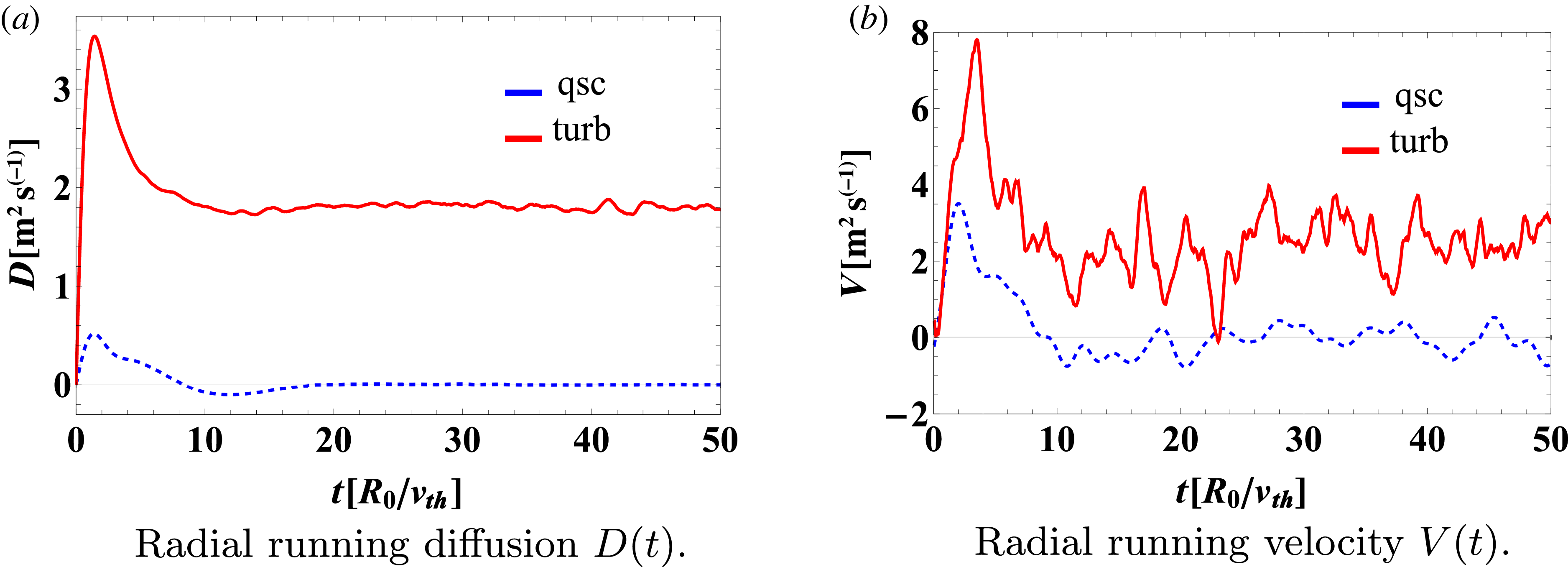
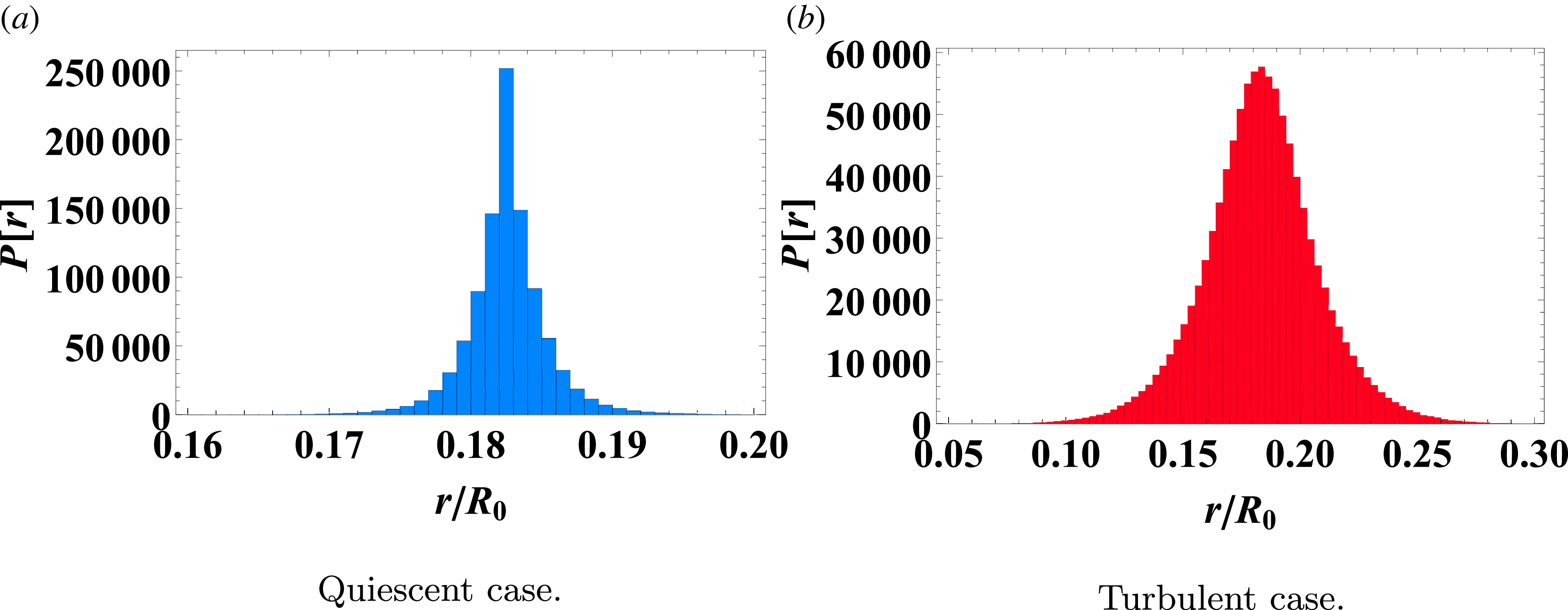


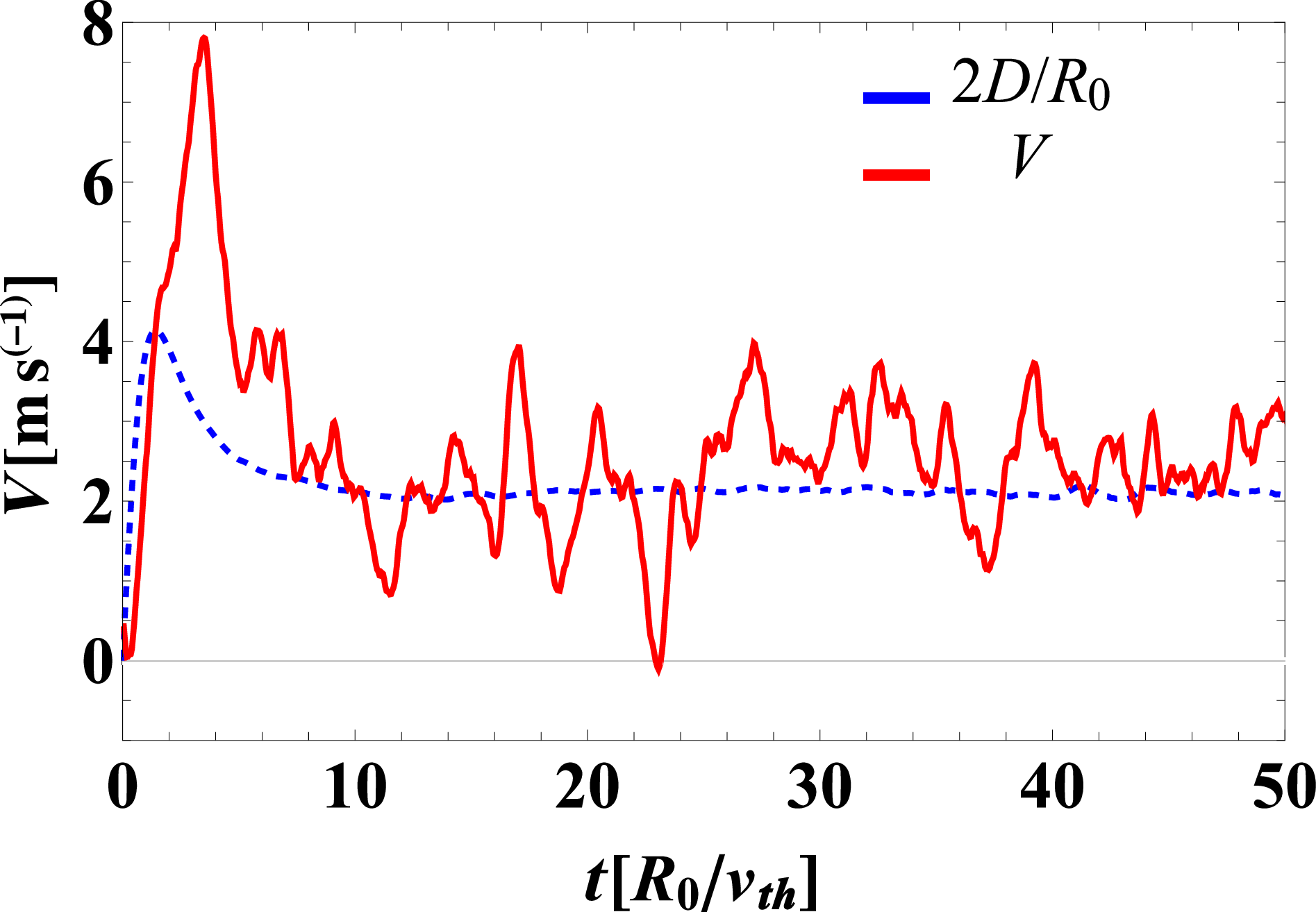


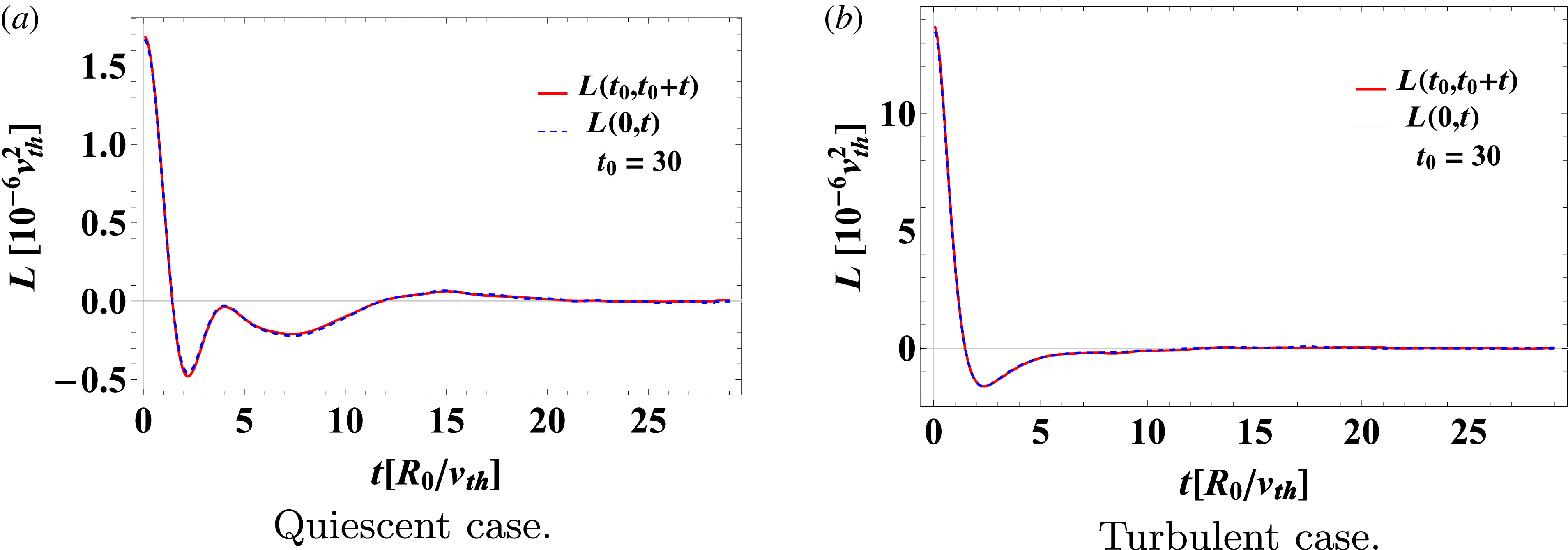


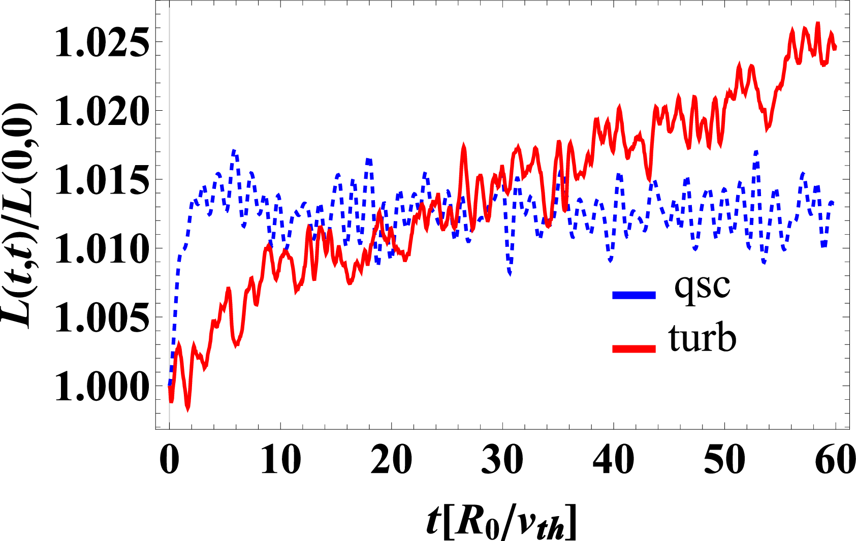


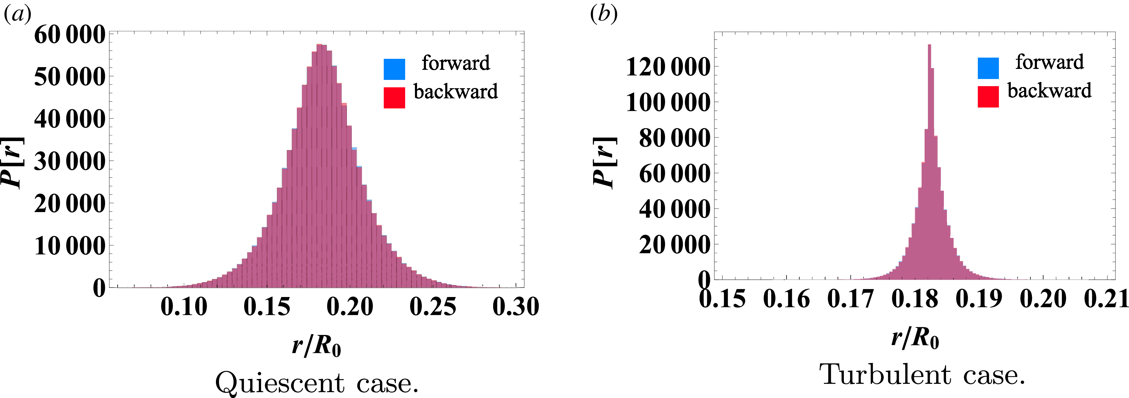

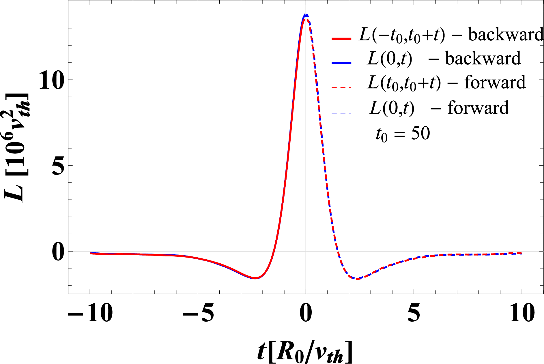


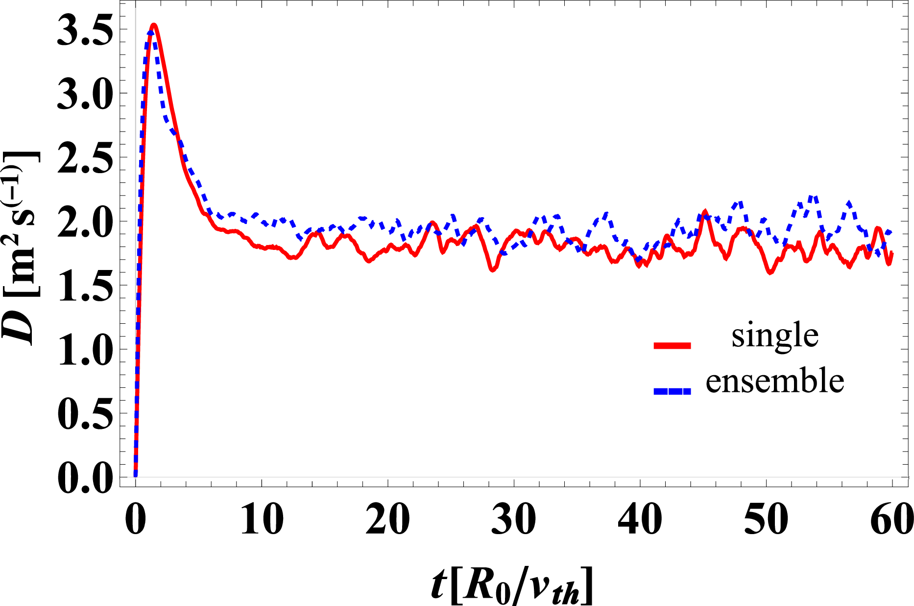

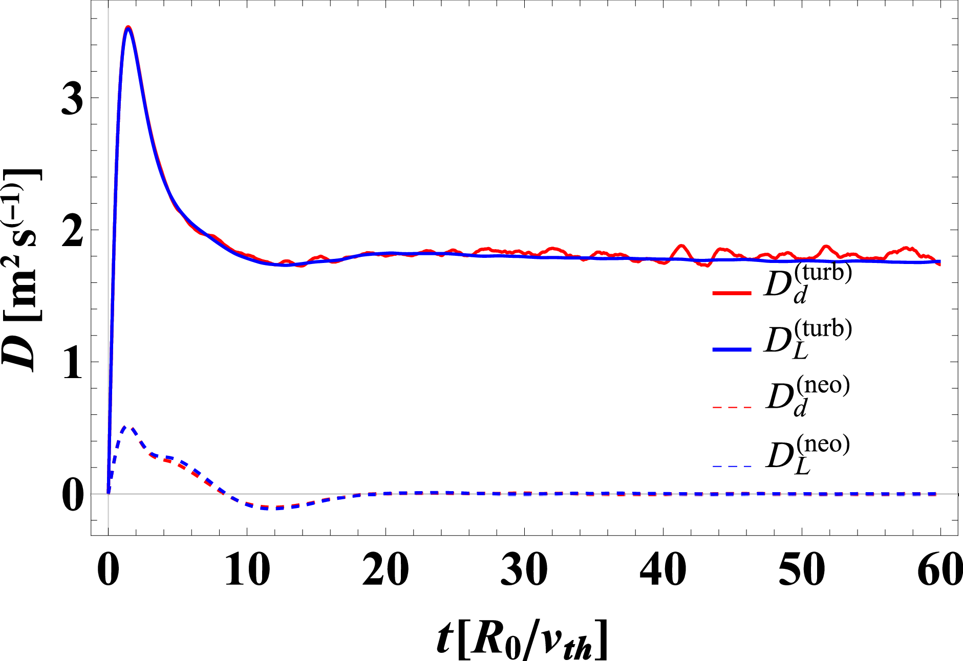


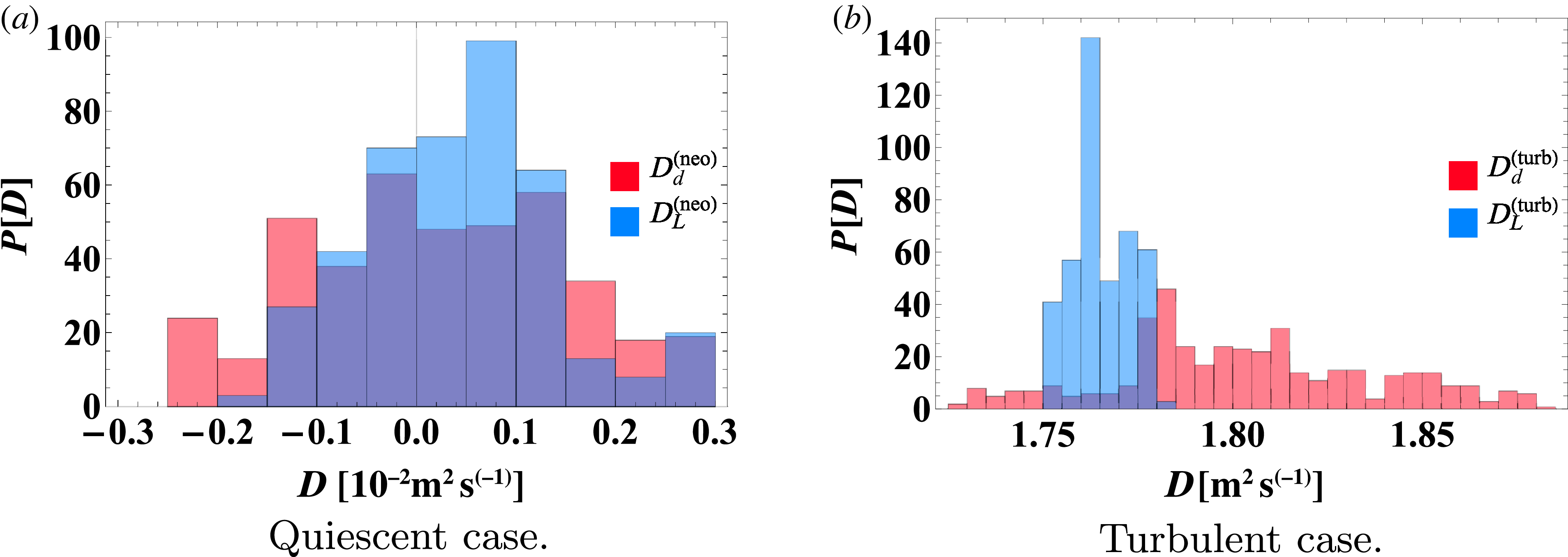


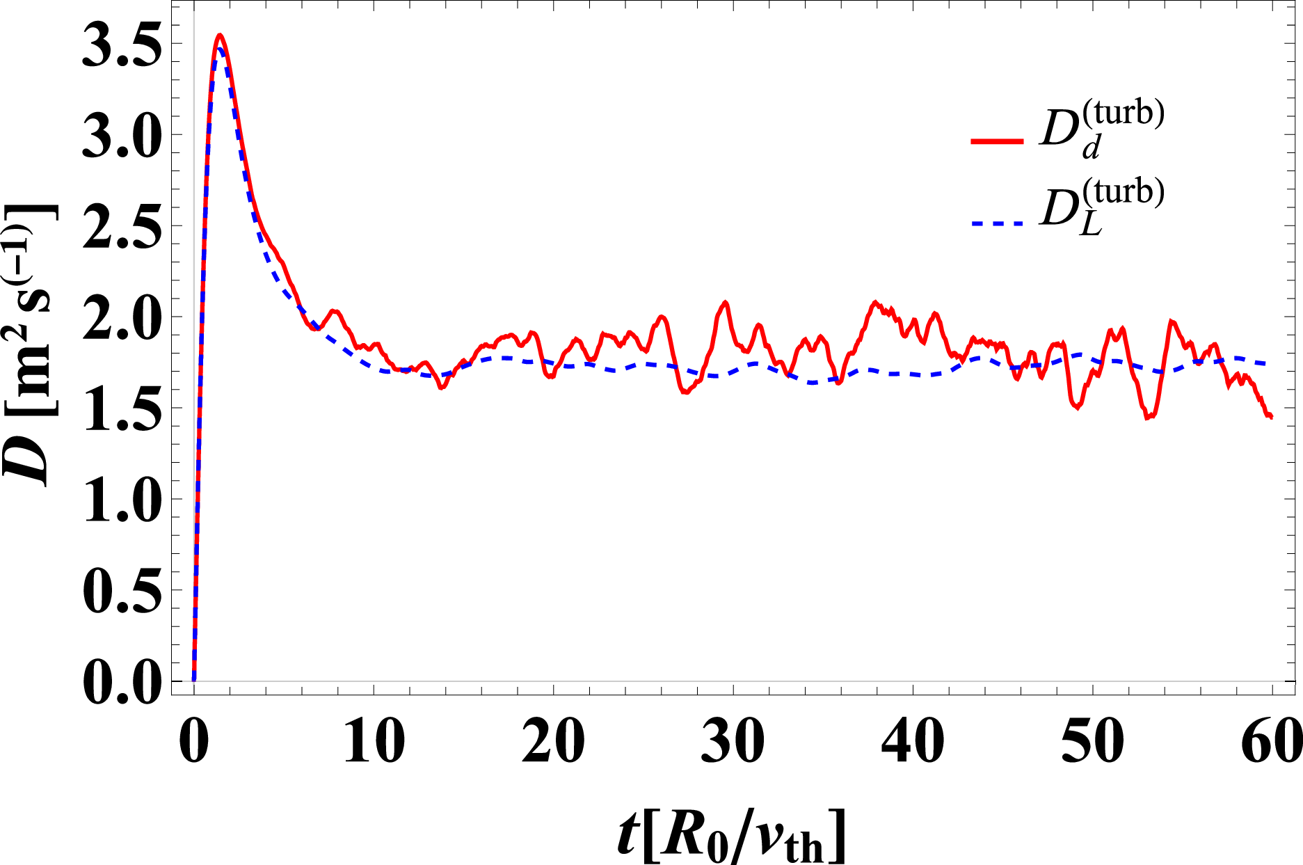

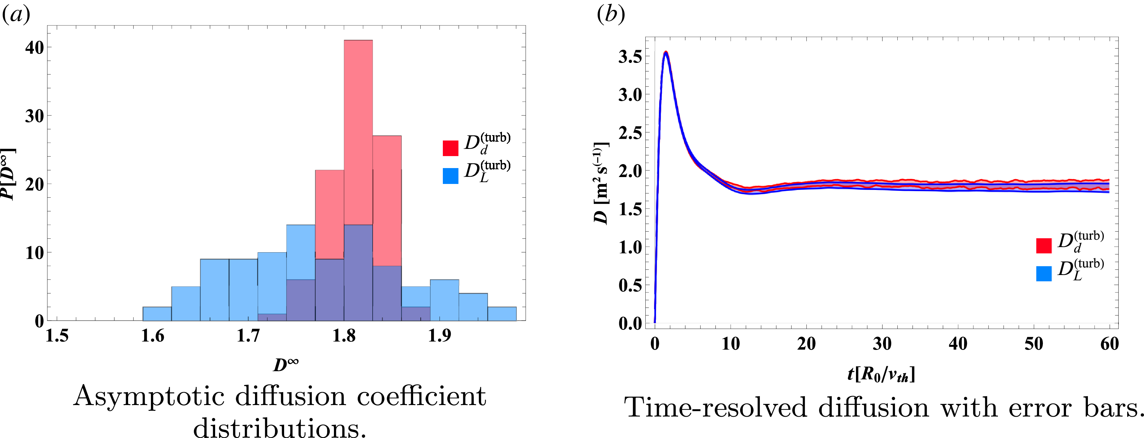


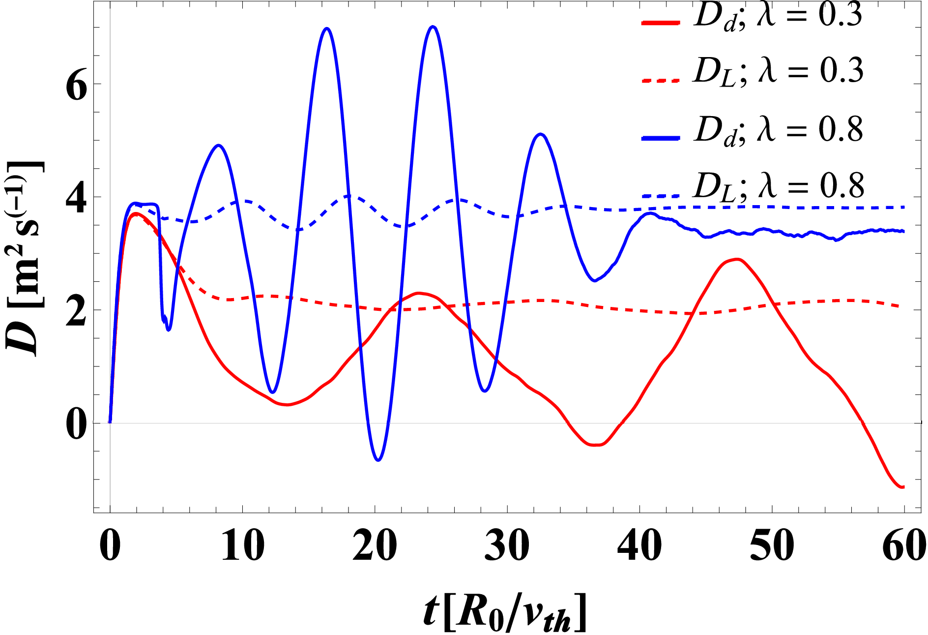


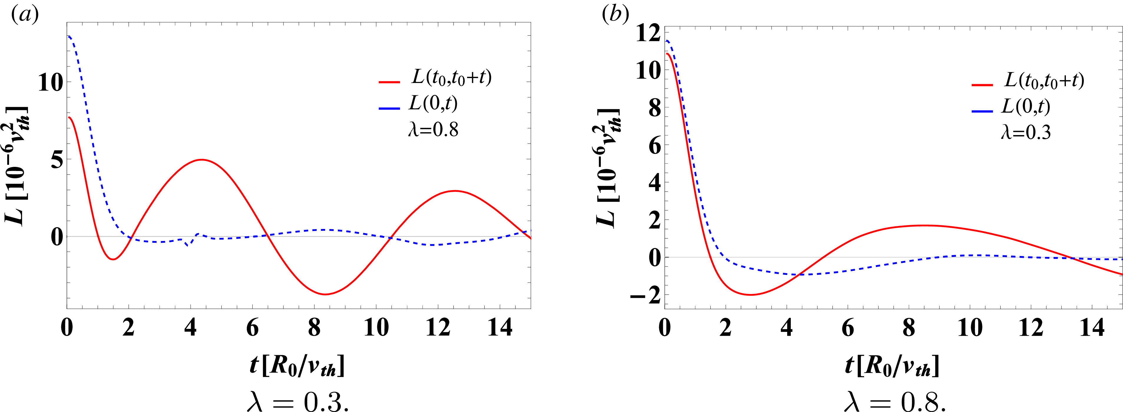


 Open access