


1. Introduction
The term self-induced transparency was first introduced in nonlinear optics, where it refers to a phenomenon occurring due to quantum interference which manifests in allowing propagation of high intensity light through an otherwise opaque medium (Kocharovskaya & Khanin Reference Kocharovskaya and Khanin1986). In nonlinear acoustics the term refers to a drop of resonant absorption for a strong acoustic wave in a fluid with bubbles, since a strong wave decreases the concentration of bubbles, such a wave can propagate without attenuation (e.g. Naugolnykh & Ostrovsky Reference Naugolnykh and Ostrovsky1998). Here, we show that, phenomenologically, somewhat similar behaviour can occur for long water waves propagating over inhomogeneous bathymetry.
It is known that, in the context of linear long water waves, transmission by a localized inhomogeneity acts as a high-pass filter, allowing short waves to pass through, while long waves are strongly reflected (e.g. Meyer Reference Meyer1975, Reference Meyer1979; Mei, Yue & Stiassnie Reference Mei, Yue and Stiassnie2005; Ermakov & Stepanyants Reference Ermakov and Stepanyants2020). However, if a long wave is weakly nonlinear, a significant share of its energy can be transferred to shorter wave scales that experience negligible reflection and cause significant changes in the reflected/transmitted energy ratio.
Long water waves exhibit a powerful scale cascade mechanism: under the combined effects of nonlinearity and dispersion, such waves tend disintegrate into a train of shorter pulses. A celebrated example is the occurrence of ‘undular bores’, observed in rivers at tidal fronts (e.g. Rayleigh Reference Rayleigh1914; Lamb Reference Lamb1932; Benjamin & Lighthill Reference Benjamin and Lighthill1954; Chanson Reference Chanson2011; and also more recent works by El, Grimshaw & Kamchatnov Reference El, Grimshaw and Kamchatnov2005; El, Grimshaw & Tiong Reference El, Grimshaw and Tiong2012 and reference therein). Undular bore-like wave patterns are a universal feature of the weakly nonlinear evolution of weakly dispersive waves, with or without inhomogeneity, encountered a wide variety of physical contests, such as nonlinear optics (e.g. Wan, Jia & Fleischer Reference Wan, Jia and Fleischer2007; Fatome et al. Reference Fatome, Finot, Millot, Armaroli and Trillo2014), flows of Bose–Einstein condensates (Xu et al. Reference Xu, Conforti, Kudlinski, Mussot and Trillo2017), internal waves in the ocean and the atmosphere (Porter & Smyth Reference Porter and Smyth2002) and many others. Their formation and evolution was studied mostly within the Korteweg–de Vries (KdV) framework (e.g. Karpman Reference Karpman1967, Reference Karpman1975; Whitham Reference Whitham1973; Gurevich & Pitayevsky Reference Gurevich and Pitayevsky1974); see also a recent review by Kamchatnov (Reference Kamchatnov2021), although it should be stressed that the dispersive shock wave (DSW) formation is a generic robust phenomenon which in the water wave context is in no way linked to any specific bathymetry. The strong gravitation of DSW studies towards the KdV is primarily due to the KdV integrability, which greatly facilitates the analysis.
Consider an initially smooth, localized elevation disturbance of the free surface, of maximum height  $a$ and characteristic length $L$, in water of characteristic depth $h_{0}$ and with the nonlinearity and dispersion parameters $\epsilon =a/h_{0}$ and $\mu =h_{0}^{2}/L^{2}$, both assumed small. If initially $\mu \ll \epsilon$, the perturbation dynamics may be approximately described as that of a Riemann wave with no dispersion (e.g. Whitham Reference Whitham1973), which evolves toward a shock wave. As the wave steepens and approaches gradient catastrophe, dispersion becomes important at the front of the wave, causing it to disintegrate into much shorter waves for which nonlinearity and dispersion are in balance. In the KdV framework, these shorter waves evolve toward KdV soliton shapes (e.g. Whitham Reference Whitham1973; Karpman Reference Karpman1975; El et al. Reference El, Grimshaw and Kamchatnov2005, Reference El, Grimshaw and Tiong2012; Kamchatnov et al. Reference Kamchatnov, Kuo, Lin, Horng, Gou, Clift, El and Grimshaw2012). In different geographical locations and different physical contexts the DSW phenomenon is known under different names (e.g. Chanson Reference Chanson2011). For obvious reasons, the general name for this process is ‘dispersive shock waves’; this term, along with its abbreviation, will be used throughout the paper. Here, we show that the disintegration of a long water wave into a DSW pattern can transfer enough energy to short scales to significantly enhance the transmission past a bathymetric inhomogeneity. Because DSWs form faster for larger amplitude waves, the DSW enhanced transmission effect is similar to the self-induced transparency in nonlinear optics (note that the physical mechanism of the phenomenon differs qualitatively from the original self-induced transparency in nonlinear optics occurring due to quantum interference discovered by Kocharovskaya & Khanin (Reference Kocharovskaya and Khanin1986)): at a bathymetric inhomogeneity, a small amplitude long wave experiences strong reflection, while a larger amplitude one is more likely to form a DSW and to blueshift its power spectrum to the range of transparency, and thus pass through.
Long water waves in the ocean susceptible to DSW self-induced transparency include, in particular, tsunamis and meteotsunamis (figure 1). Tsunamis are usually generated in the deep ocean, primarily by earthquakes or volcanic activity. Due to their characteristic dimensions (length  $L\sim 10^2$ km, amplitude $a\sim 1$ m) tsunamis generated in the deep ocean evolve over the open ocean effectively as linear waves and may develop a DSW only on the shelf (e.g. Madsen, Fuhrman & Schäffer Reference Madsen, Fuhrman and Schäffer2008). In contrast, meteotsunamis are usually much shorter waves ( $L\sim 10\ {\rm km}, a\sim 0.5\ {\rm m}$), typically generated on the continental shelf by atmospheric perturbations through the Proudman resonance (e.g. Proudman Reference Proudman1929; Rabinovich & Monserrat Reference Rabinovich and Monserrat1996, Reference Rabinovich and Monserrat1998; Monserrat, Vilibić & Rabinovich Reference Monserrat, Vilibić and Rabinovich2006; Vilibić, Monserrat & Rabinovich Reference Vilibić, Monserrat and Rabinovich2014; Pellikka et al. Reference Pellikka, Šepić, Lehtonen and Vilibić2022). To give a rough idea of characteristic scales of DSW formation consider a constant shelf slope of $5\times 10^{-4}$, table 1 shows characteristic parameters for the evolution of a 1 m height tsunami entering the shelf at 100 m depth, and a 0.5 m amplitude meteotsunami generated near the 50 m isobath. In spite of large difference in scales, estimates of the gradient catastrophe location obtained using the nonlinear shallow water equations with no dispersion are similar for tsunamis and meteotsunamis waves. Note that the DWS disintegration occurs before the gradient catastrophe. Table 1 suggests that both tsunamis and meteotsunalis develop a DSW structure on the shallow shelf, before reaching the near-shore slope (typically of the order of ${\sim }10^{-2}$).
Examples of tsunami and meteotsunami DSWs. (a) Fukushima tsunami (2011) at Kuji Port, Iwate Prefecture, Japan; frame 1 : 20 min from video posted by Kamaishi Port Office and Ministry of Land, Infrastructure, Transport and Tourism (MLIT) (2011). The tug boat length is  $\approx$20 m long (visual estimation). (b) Meteotsunami DSW or solibore recorded in near the 8 m isobath on the Atchafalaya shelf, LA, USA (Sheremet, Gravois & Shrira Reference Sheremet, Gravois and Shrira2016).

Characteristic scales of tsunamis and meteotsunamis on the shelf of slope  ${\approx }5\times 10^{-4}$ (Madsen et al. Reference Madsen, Fuhrman and Schäffer2008; Sheremet et al. Reference Sheremet, Gravois and Shrira2016); $T$,
$T$,  $L$ and $a$ are the characteristic wave period, length and amplitude scales; $\epsilon$ and $\mu$ are the nonlinearity and dispersion parameters; $\sigma^2=\epsilon/\mu$ is the Ursell number; $h$ is the depth at wave origin (shelf edge for tsunamis); $h_{c}$ is the depth at the location of gradient catastrophe estimated ignoring dispersion.

The shoreline hazard posed by long waves such as tsunamis and meteotsunamis depends critically on the processes affecting their propagation from the deep ocean onto the shallow near-shore shelf. While DSW solitons are a hazard in their own right, as illustrated in figure 1(a) by the precarious pitch of the tugboat attempting to evade them, the increased transmission of energy due to the DSW self-induced transparency may play a significant role in the shoreline impact of the wave and is the focus of our study.
To the best of our knowledge, the DSW self-induced transparency has never been studied. The main aim of the work is to elucidate its mechanism employing the maximally simplified setting. The simplest, but still adequate, mathematical model able to capture the essence of the phenomenon by taking into account weak nonlinearity, weak dispersion and bathymetry, is the Boussinesq equations (e.g. Peregrine Reference Peregrine1967; Dingemans Reference Dingemans1997). It is relatively straightforward to simulate the Boussinesq equations numerically, and there are available reliable established codes, e.g. FUNWAVE-TVD (Kirby et al. Reference Kirby, Wei, Chen, Kennedy and Dalrymple1998). However, untangling and accounting for the roles of nonlinearity, dispersion and interaction with localized bathymetric inhomogeneity poses a significant challenge – even upon restricting the wave dynamics to one-dimensional, non-breaking regimes of propagation over a frictionless bottom. Reconstructing the general picture of the phenomenon from numerical simulations using realistic, comprehensive wave physics is problematic, due to the large number and range of required parameters.
The main difficulty of the problem is in the apparent necessity of simultaneous handling of wave nonlinear dynamics and reflection/transmission. To fix the idea, we consider here an idealized model of bathymetry, which enables us to spatially separate the effects of nonlinearity and dispersion, on the one hand, and of bathymetry, on the other. This makes it easier to get a quantitative description of the phenomenon for the chosen bathymetry and, crucially, to provide an overall qualitative picture. It also helps to clarify the particular roles of the mechanism's essential components: DSW formation and reflection. Our approach is a posteriori validated by comparison with an established numerical model, FUNWAVE-TVD (Kirby et al. Reference Kirby, Wei, Chen, Kennedy and Dalrymple1998).
In § 2 we provide the mathematical formulation of the problem and discuss the mathematical and the numerical tools we use. The relevant aspects of the DSW evolution over even bottom are discussed in § 3. The results of the analysis are presented in § 4 and briefly summarized in § 6. Section 5 discusses the robustness of the phenomenon and its modelling with respect the underlying assumptions. The Appendix compares our results with FUNWAVE-TVD simulations.
2. Formulation of the problem
2.1. Basic equations, assumptions and simplifications
We consider the evolution of weakly nonlinear long waves over bathymetry within the framework the Boussinesq system of equations (e.g. Peregrine Reference Peregrine1967; Whitham Reference Whitham1973; Karpman Reference Karpman1975; Dingemans Reference Dingemans1997; Mei et al. Reference Mei, Yue and Stiassnie2005). We confine our attention to non-breaking regimes. There are many asymptotically equivalent formulations of the Boussinesq equations, however, in the context of this work, the differences between various versions are immaterial. For simplicity only, we consider a one-dimensional geometry. For certainty, we choose
 \begin{equation} \eta_{t}+[\left(h+\eta\right)u]_{x}=0,\quad u_{t}+g\eta_{x}+uu_{x}=\tfrac{1}{2}h\left[\left(hu\right)_{xx}-\tfrac{1}{3}hu_{xx}\right]_{t},\end{equation}
where  $\eta (x,t)$ is the free surface elevation, $x$ is the horizontal coordinate, $t$ is time, $u$ is the vertically averaged horizontal velocity, $h(x)$ is the bathymetry, $g$ is the gravitational acceleration and the subscripts $x$ and $t$ denote partial derivatives.
The Boussinesq equations (2.1a,b) describe both left- and right-propagating waves, as well as their interactions, and therefore provide a full description of wave scattering by inhomogeneities of topography. Often physics allows for considering only left- or right-propagating waves alone, then all the variety of formulations of the Boussinesq equations can be simplified to the same KdV equation with variable coefficients (e.g. Ostrovsky & Pelinovsky Reference Ostrovsky and Pelinovsky1975)
 \begin{equation} \eta_{t}\pm \sqrt{gh}\left(1 +\frac{3\eta}{2h}\right) \eta_x + \frac{h}{6g}\eta_{xxx} +\frac{\sqrt{gh}}{4h}h_x\eta=0 . \end{equation}
Since the aim of the work is to elucidate the mechanism of the DSW self-induced transparency in the simplest possible setting, we choose a strongly idealized model of bathymetry which will allow us to use the KdV equation for a considerable part of the domain. This simplification is ostensibly inapplicable when the reflection is not negligible, not only because the reflection implies bidirectional propagation, but also because the outcome of wave evolution propagating in any direction may be modified by the weak interaction with the counter-propagating waves. To validate the use of the adopted KdV reduction we use a well-established numerical model, FUNWAVE-TVD (Wei et al. Reference Wei, Kirby, Grilli and Subramanya1995; Kirby et al. Reference Kirby, Wei, Chen, Kennedy and Dalrymple1998; Shi et al. Reference Shi, Kirby, Tehranirad, Harris, Choi and Malej2016) in the Appendix.
Because this is the first study of the long wave DSW self-induced transparency with the prime aim of understanding the nature of the process, we focus on the two key components of the mechanism: weak nonlinearity and reflection. This implies neglecting all other processes likely to occur at the near shore, such as wave breaking, wave–current interaction, bottom friction and others. We also leave aside three-dimensional aspects of the wave dynamics, which are not essential for fixing the idea.
Even in the basic Boussinesq representations in the strictly two-dimensional setting (2.1a,b) the interplay of nonlinearity, dispersion and inhomogeneity in the wave evolution is usually too complex to be described analytically. Even with numerical models, it is not straightforward to deconstruct it into its basic mechanisms. The KdV equation has provided much of the analytical understanding of the DSW process (e.g. Whitham Reference Whitham1973; Gurevich & Pitayevsky Reference Gurevich and Pitayevsky1974; Karpman Reference Karpman1975; El et al. Reference El, Grimshaw and Kamchatnov2005, Reference El, Grimshaw and Tiong2012; El & Hoefer Reference El and Hoefer2016; Kamchatnov Reference Kamchatnov2021).
2.2. Bathymetry model: the decoupling hypothesis
Remarkably, separating reflection from nonlinearity is a plausible approximation in many real conditions. The basis for this is the observation that ocean topography is often characterized by significant bathymetric inhomogeneity separated by relatively flat areas. For example, the continental slope separating the abyssal plane and the shelf; the pattern repeats itself for smaller scales closer to the shoreline. For brevity only, we refer to the flat areas as ‘shelves’, and the inhomogeneity as ‘slopes’, irrespective of the scales.
For oceanic long waves we consider, the bottom slopes are typically steep in the following sense: for example, for the meteotsunami scales given in table 1, a near-shore slope of 0.01 corresponds to the commonly used ‘mild slope parameter’ of order one (Mei et al. Reference Mei, Yue and Stiassnie2005). Over such a steep slope, wave evolution is fast compared with the time scale of nonlinearity, the nonlinear interaction between the incoming and reflected waves to leading order is negligible and wave reflection then is approximately linear. If in addition the long wave is localized, the counterpropagating waves are passing through each other too quickly for nonlinear effects to accumulate. Thus, there are situations where the reflected wave can be effectively decoupled from the nonlinear evolution of the incoming wave.
With this observation, the DSW reflection problem greatly simplifies. Rather than considering a Boussinesq system for waves propagating in two opposite directions, we can solve instead a unidirectional KdV initial value problem. The reflected wave may now be computed ‘offline’, as a postprocessing result, using existing linear reflection models (e.g. Ermakov & Stepanyants Reference Ermakov and Stepanyants2020). The validity of this simplifying assumption may be verified using the FUNWAVE-TVD numerical model (see the Appendix). To eliminate entanglement of DSW evolution and shoaling effects, we choose a particular profile of the bathymetry: a shelf of constant depth  $h_{2}$ extending for an arbitrary distance towards a slope that transitions to another shallow shelf of constant depth $h_{1}$; for certainty, for now let $h_{1}< h_{2}$ (figure 2a). Because the reflection process is not directly related to DSW evolution, the toe of the slope may be placed at any location on the shelf $h_{1}$, and the reflected wave may be computed at any stage of the DSW evolution.
(a) Schematics of simplified reflection/transmission problem for a weakly nonlinear positive perturbation. The perturbation propagates over a shelf of constant depth  $h_{1}$. The slope from $h_{2}$ to $h_{1}$ is assumed to be steep in the sense that the interaction between incoming and reflected waves may be neglected. The problem reduces to the well-understood KdV evolution of a DSW over a flat bottom, with the reflected wave computed in postprocessing, and may be computed for any DSW evolution stage. (b) Bathymetry settings for reflection/transmission coefficients, reproduced from Ermakov & Stepanyants (Reference Ermakov and Stepanyants2020). The direction of the depth variation is irrelevant.

2.3. Reflection and transmission at a constant slope
By virtue of negligible reflection for linear waves in the WKB (Wentzel–Kramers– Brillouin) asymptotic regime, it has long been known that, for linear waves, a bathymetric inhomogeneity acts as a high-pass filter, therefore, in this section we confine our discussion to reflection and transmission of longer wave components. In the linear settings, this is equivalent to reducing the linearized Boussinesq system to the classical non-dispersive linear shallow water equations. A comprehensive discussion of linear reflection of non-dispersive waves by several analytic slope shapes is given in Ermakov & Stepanyants (Reference Ermakov and Stepanyants2020) (see also references therein). Here, we just provide a brief overview of reflection by a constant slope, but the results are of general applicability.
In the framework of the linearized shallow water equations in the standard notation, where  $u$ and $\eta$ are particle velocity and free surface elevation, $x$ and $t$ are the horizontal coordinate and time, while $h(x)$ and $g$ are the local depth and acceleration due to gravity
 \begin{equation} \eta_{t}+u_{x}h+uh_{x}=0,\quad u_{t}+g\eta_{x}=0.\end{equation}
The solution for a bathymetry consisting of two shelves of  $h_{1}$ and $h_{2}$ separated by a constant slope $\alpha =({h_{2}-h_{1}})/{L_{12}}$ (figure 2b) may be sought as a Fourier summation of monochromatic time solutions. For a single harmonic of frequency $\omega$, (2.3a,b) reduce over the slope to the Bessel equation with the known general solution
 $$\begin{gather} \eta =\alpha L_{12}\frac{{\rm i}}{\varpi}\left[A{\rm J}_{0}\left(2\varpi\sqrt{\xi}\right)+ B{\rm Y}_{0}\left(2\varpi\sqrt{\xi}\right)\right]{\rm e}^{{\rm i}\varpi\tau}. \end{gather}$$
 $$\begin{gather}u =\frac{L_{12}}{T_{12}}\frac{1}{\varpi\sqrt{\xi}}\left[A{\rm J}_{1}\left(2\varpi\sqrt{\xi}\right)+ B{\rm Y}_{1}\left(2\varpi\sqrt{\xi}\right)\right]{\rm e}^{{\rm i}\varpi\tau}, \end{gather}$$
where  ${\rm J}_{n}$ and ${\rm Y}_{n}$ are the Bessel functions of the first and second kinds, $A$,
$A$,  $B$ are arbitrary constants and variables $x=L_{12}\xi$, $h=h_{1}-\alpha L_{12}\xi$ and the angular frequency $\varpi =\omega T_{12}$, are scaled using the length of the slope $L_{12}$ and the slope time scale
 \begin{equation} T_{12}=\sqrt{\frac{L_{12}}{\alpha g}}.\end{equation}
 The complete solution is obtained by matching the solution (2.4)–(2.5) at the slope toe/top  $x_{1,2}$ with monochromatic waves propagating in both directions of the two shelves. This yields reflection and transmission coefficients
 $$\begin{gather} \mathcal{R}_{\uparrow}=\frac{z_{J1}^{*}z_{Y2}^{*}-z_{J2}^{*}z_{Y1}^{*}}{z_{J1}^{*}z_{Y2}-z_{J2}z_{Y1}^{*}};\quad\mathcal{T}_{\uparrow}=\frac{z_{J1}^{*}z_{Y1}-z_{J1}z_{Y1}^{*}}{z_{J1}^{*}z_{Y2}-z_{J2}z_{Y1}^{*}}, \end{gather}$$
 $$\begin{gather}\mathcal{R}_{\downarrow}=\frac{z_{J1}z_{Y2}-z_{J2}z_{Y1}}{z_{J1}^{*}z_{Y2}-z_{J2}z_{Y1}^{*}};\quad \mathcal{T}_{\downarrow}=\frac{z_{J2}^{*}z_{Y2}-z_{J2}z_{Y2}^{*}}{z_{J1}^{*}z_{Y2}-z_{J2}z_{Y1}^{*}}, \end{gather}$$
for waves propagating upslope ( $\uparrow$), and downslope ( $\uparrow$), where
 \begin{align} z_{Jn}={\rm J}_{0}\left(2\varpi\sqrt{\xi}_{n}\right)+{\rm i}{\rm J}_{1}\left(2\varpi\sqrt{\xi}_{n}\right);\quad z_{Yn}={\rm Y}_{0}\left(2\varpi\sqrt{\xi}_{n}\right)+{\rm i}{\rm Y}_{1}\left(2\varpi\sqrt{\xi}_{n}\right),\end{align}
and the asterisk denotes complex conjugation.
The reflected waves are found by using expressions (2.7a,b)–(2.8a,b) and the Fourier transform of the incoming wave
 \begin{align} \varphi_{R}(t)=\int_{-\infty}^{\infty}\mathcal{R}(\,f)\hat{\varphi}(\,f)\exp({2{\rm \pi} {\rm i}ft})\,{\rm d}f,\quad \text{where}\ \hat{\varphi}(\,f)=\int_{-\infty}^{\infty}\varphi(t)\exp({-2{\rm \pi} {\rm i}ft})\,{\rm d}t,\end{align}
where the subscript  $R$ denotes the reflected wave. For the transmitted component one has to replace $\mathcal {R}$ with $\mathcal {T}$ and the subscript $R$ with the subscript $T$. The reflected and transmitted fractions of the incoming energy flux are given by the expressions
 \begin{equation} F_{R}=\int_{-\infty}^{\infty}\frac{1}{2}\left|\hat{\varphi}_{R}(\,f)\right|^{2}\,{\rm d}f\quad \text{and}\quad F_{T}=\sqrt{\frac{h_{1}}{h_{2}}}\int_{-\infty}^{\infty}\frac{1}{2}\left|\hat{\varphi}_{T}(\,f)\right|^{2}\,{\rm d}f,\end{equation}
valid both for the upslope and downslope propagation.
The absolute values of the coefficients do not depend on the direction of propagation:  $|\mathcal {R}_{\uparrow }|=|\mathcal {R}_{\downarrow }|$ and $|\mathcal {T}_{\uparrow }|=|\mathcal {T}_{\downarrow }|$. The reflection and transmission coefficients given by (2.7a,b) satisfy the conservation of energy, in the sense that the energy flux of the incoming wave is equal to the sum of the energy fluxes of the reflected and transmitted waves, $|\mathcal {R}|^{2}+|\mathcal {T}|^{2}\sqrt {{h_{1}}/{h_{2}}}=1$ (direction subscript omitted). In this relation, $|\mathcal {R}|^{2}$ may be interpreted as the fraction of the energy flux reflected by the slope, and $|\mathcal {T}|^{2}\sqrt {{h_{1}}/{h_{2}}}$ represents the fraction of the incoming energy flux transmitted past the slope. Figure 3 shows the reflected and transmitted energy flux fractions for ${h_{2}}/{h_{1}}=50$; downslope and upslope energy flux fractions have identical frequency distributions for the same ratio of depths. In the long wave limit, the reflection and transmission coefficients take the well-known forms (Mei et al. Reference Mei, Yue and Stiassnie2005; constant gain, no phase shift)
 \begin{equation} \mathcal{R}(0) \sim\frac{\sqrt{\xi_{2}}-\sqrt{\xi_{1}}}{\sqrt{\xi_{1}}+\sqrt{\xi_{2}}},\quad \mathcal{T}(0)\sim\frac{2\sqrt{\xi_{2}}}{\sqrt{\xi_{1}}+\sqrt{\xi_{2}}}.\end{equation}
Reflected and transmitted fractions of energy flux for monochromatic wave by a constant slope for  $h_{2}/h_{1}=50$ (log scale; see also figure 2b). The reflected fraction is below 10 % for all frequencies greater than $0.4\ T_{12}^{-1}$ (2.6). The reflection coefficient decays roughly as $f^{-2}$ outside the red box, where $f$ is the scaled frequency.
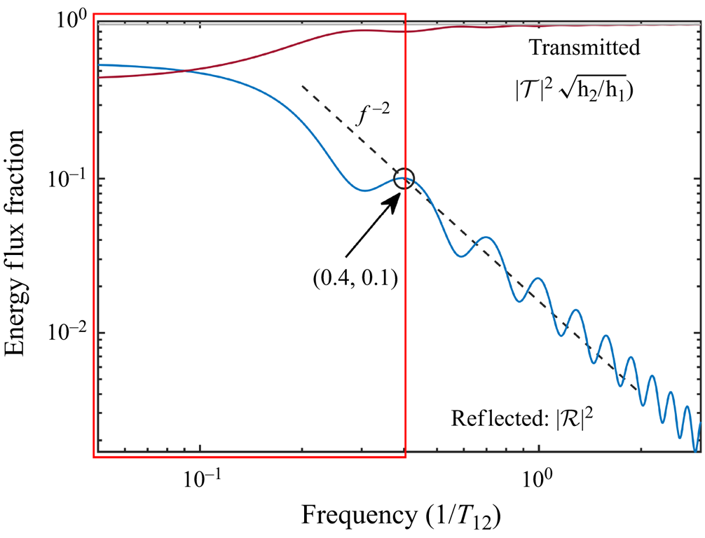
The reflected energy fraction falls below 10 % for the frequencies exceeding 0.4  $T_{12}^{-1}$ (outside the red box in figure 3). Figure 3 illustrates the statement that reflection and transmission processes may be described as dual linear low- and high-pass filters, with the spectral response given by (2.7a,b)–(2.8a,b). This is consistent with our consideration of reflection within the framework of the shallow water equation, neglecting high frequency dispersion.
3. Dispersive shock wave formation and evolution over constant depth
As discussed in § 2.2, here, we are concerned with the evolution of localized perturbations over a flat shelf prior to encountering the bathymetric inhomogeneity. As we argued above, at this stage of wave evolution it is legitimate to confine our consideration to unidirectional propagation. Then all versions of the Boussinesq system can be reduced to a single KdV equation. Recasting this KdV equation in non-dimensional ‘signalling’ coordinates (e.g. Karpman Reference Karpman1975; Osborne Reference Osborne1975; Caputo & Stepanyants Reference Caputo and Stepanyants2003)
 \begin{equation} \varphi_{\xi}+\varphi\varphi_{\tau}+\frac{1}{\sigma^{2}}\varphi_{\tau\tau\tau}=0,\end{equation}
gives an initial value problem with initial condition
 \begin{equation} \varphi(0,\tau)=\varphi_{0}(\tau);\quad\varphi(\xi>0,0)=0,\end{equation}
where the space and time variables  $x=\frac {a}{T}\xi$ and $t=T\tau$ are scaled using the characteristic time scale $T$ of the initial perturbation, the parameter $\sigma ^{2}={\epsilon }/{\mu }$ is the Ursell number and $\epsilon ={a}/{h}$ and $\mu ={h^{2}}/{L^{2}}$, with $L=3cT$ and $c=\sqrt {gh}$. Equation (3.1) is known to have an infinite number of conserved quantities (e.g. Miura, Gardner & Kruskal Reference Miura, Gardner and Kruskal1968; Whitham Reference Whitham1973; Karpman Reference Karpman1975) of the form
 \begin{equation} Q_{m}=\int_{-\infty}^{\infty}q_{m}(\eta)\,{{\rm d}\kern0.06em x},\quad m=1,2,\ldots\end{equation}
where  $q_{m}$ are polynomials of order $m$ in $q$ and may contain its spatial derivatives. Depending on the meaning of the function $\varphi$, the lowest orders $q_{1}=\varphi$, $q_{2}=\varphi ^{2}/2$ may be interpreted as the densities of mass and momentum (e.g. Drazin & Johnson Reference Drazin and Johnson1989), or momentum and energy (e.g. Dingemans Reference Dingemans1997). We chose here the latter interpretation. Note, however, that $q_2$ is used here only to evaluate the distribution over the DSW disintegration products; the exact relationship between these quantities and the actual form of water wave momentum and energy (e.g. Ablowitz & Segur Reference Ablowitz and Segur1979) is not important for this study.
The equation is exactly solvable by the inverse scattering transform technique (e.g. Whitham Reference Whitham1973; Karpman Reference Karpman1975; Ablowitz & Segur Reference Ablowitz and Segur1981) and other methods. Solitons of the form  $\varphi \propto \operatorname {sech}^{2}$ play a fundamental role in the solution of the Cauchy problem: solitons emerge as the large-time asymptotics of any initially localized perturbation of positive polarity. Equation (3.1) is scaled in such a way that the scale of a soliton of (3.1) corresponds to $\sigma _{s}^{2}=12$. If $\int _{-\infty }^{\infty }\varphi _{0}(\tau )\,{\rm d}\tau \geq 0$, the initial pulse disintegrates into a number of solitons and a dispersive tail. If the disturbance $\varphi _{0}$ is such that, $\sigma ^{2}\gg \sigma _{s}^{2}$, then, initially, the wave evolves as a Riemann simple wave without dispersion: the front steepens, then a shock wave begins to form. However, as the wave front approaches the gradient catastrophe, at the front of the wave dispersion becomes important, causing the wave to disintegrate into wave groups that eventually transform into solitons, that is, the DSW is formed. For the self-induced transparency phenomenon, of most interest are the cases with large $\sigma$ that can generate $N\gg 1$ solitons, where
 \begin{equation} N\approx \frac{\sigma}{{\rm \pi}\sqrt{6}}\int_{\varphi(\xi)>0}\sqrt{\varphi(\xi)}\,{\rm d}\xi.\end{equation}
Note that an arbitrary small perturbation will always generate at least one soliton if  $\int _{-\infty }^{\infty }\varphi _{0}(\tau )\,{\rm d}\tau >0$ and, crucially, if the evolution domain is large enough.
These theoretical results are valid for infinite time and infinite extent of the horizontal segment, which is often far from realistic situations. Nevertheless, these results enable us to get important a priori bounds on reflected and transmitted energy, which we will briefly discuss in § 5.
For an initial disturbance (3.2a,b) of the form
 \begin{equation} \varphi_{0}(\tau)=a\operatorname{sech}^{2}\frac{\tau-\tau_{0}}{T},\end{equation}
the analytical solution for large time is known (e.g. Karpman Reference Karpman1967, Reference Karpman1975). It does not include any dispersive wave residual, and the number and amplitude of the solitons produced are
 \begin{align} \frac{a_{n}}{a}=\frac{3}{\sigma^{2}}\left[1+\sqrt{1+\frac{2}{3}\sigma^{2}}-2n\right]^{2},\quad \text{with}\ n=1,2,\ldots,N<\frac{1}{2}\left(1+\sqrt{1+\frac{2}{3}\sigma^{2}}\right).\end{align}
The nth soliton in the sequence carries the values of the mth conservation integral  $Q_{m,n}$ as follows:
 \begin{equation} Q_{m,n}=\sqrt{\frac{12}{\sigma^{2}}}\frac{2^{m}\left[\left(m-1\right)!\right]^{2}}{2m-1}a_{n}^{{\left(2m-1\right)}/{2}}.\end{equation}
These results will be used below for a priori estimates from above for the outcome of the DSW evolution and transmission.
4. Reflection of a DSW at a constant slope
4.1. Simulations
The asymptotic state of the disintegration of a DSW is well understood (e.g. Whitham Reference Whitham1973; Gurevich & Pitayevsky Reference Gurevich and Pitayevsky1974; Karpman Reference Karpman1975; Caputo & Stepanyants Reference Caputo and Stepanyants2003; El et al. Reference El, Grimshaw and Kamchatnov2005, Reference El, Grimshaw and Tiong2012; Kamchatnov et al. Reference Kamchatnov, Kuo, Lin, Horng, Gou, Clift, El and Grimshaw2012; Kamchatnov Reference Kamchatnov2021). However, the reflection by an inhomogeneity can occur during transient states of the DSW disintegration, well before the wave reaches its asymptotic state. At present, numerical simulations are the only approach available for investigating this problem.
The KdV equation (3.1) is integrated for initial conditions of the form given in (3.5) using a symmetric split step method that combines the time Fourier transform with a fourth-order Runge–Kutta integration of the nonlinear term (Sheremet et al. Reference Sheremet, Gravois and Shrira2016). In all simulations presented here, the relative error for the energy flux was  ${<}10^{-7}$.
The reflected and transmitted waves are calculated using the linear model discussed in § 2.3 for the toe of the slope located at positions ranging from the position of the initial perturbation to the full extent of the integration domain. This provides an estimate of the DSW reflection process at all simulated evolution stages.
The effect of the DSW disintegration on reflection is determined primarily by two time scales: the reflection time scale  $T_{12}$ (specified by (2.6)) and the characteristic time scale $T$ of the wave itself. The frequency band allowed by the reflection and transmission filters (2.7a,b)–(2.8a,b) depends on the relation between these two time scales. For sufficiently gentle or too steep slopes $\alpha$, i.e. $T\ll T_{12}$ or $T\gg T_{12}$, the contribution of the DSW to transmission is small, because the initial perturbation is either almost entirely transmitted or nearly entirely reflected. Therefore, the maximum effect of the DSW on transmission occurs for the waves of time scales comparable to the reflection time scale, i.e. $T\sim T_{12}$.
As a reference example in the meteotsunami context, consider an initial positive perturbation of the form given in (3.5) of  $L\approx 3.3$ km width and time scale $T=150$ s, starting its propagation either towards the shoreline or in the opposite direction at a shelf of depth $h=50$ m, which implies $\mu =2.5\times 10^{-5}$. A wave height of $a=1$ m corresponds to $\epsilon =0.02$, and $\sigma ^{2}=795$, In the absence of dispersion, such a wave would reach the gradient catastrophe point after propagating over a distance of ${\approx }40\ L$, or $\approx$134 km; by virtue of (3.6), its disintegration can produce at most 12 solitons. The reflected and transmitted components are calculated below for an upslope transition from 50 to 1 m depth (similar to the reflection at an inner shelf and beach), and a downslope transition from 50 to 1000 m. The 1 m and 1000 m depths only determine the values of the long wave coefficients ((2.11a,b); i.e. the scale of the $\mathcal {R}(\,f)$ function), but otherwise have no effect on the shape of the reflected and transmitted waves.
Figure 4 shows the reflected fraction of the energy flux for different upslope values. Downslope reflection has a similar dependence on the slope (not shown). The maximum effect of the DSW disintegration on reflection occurs for slopes 0.01 $\leq \alpha \leq 0.02$ for upslope propagation, and for 0.05 $\leq \alpha \leq 0.1$ for downslope propagation.
Dependence of the reflected fraction of energy flux for a monochromatic wave on the slope (see figure 2a). The reflection coefficient is plotted as a function of the time scale (inverse period) of the wave. A comparison with figure 3 suggests that  $T\approx T_{12}$ for slope $\alpha =0.015$.

4.2. Simulation results
The results of the simulations are presented below for two reference waves of initial amplitude 0.5 m and 1.0 m, corresponding to  $\sigma ^{2}=397$ and $\sigma ^{2}=795$, respectively. The simulations were carried out assuming the slope value $\alpha \approx 0.015$ for upslope propagation (blue line in figure 4), which is a rather typical value for the USA Atlantic inner shelf. For downslope propagation we set the slope $\alpha =0.07$.
The energy transfer away from the strong reflection spectral band (indicated by red rectangle, figures 3 and 4), which is the basis of the self-induced transparency phenomenon, may be caused not just by the DSW formation and evolution, but also by simple nonlinear steepening of the initial perturbation. Before shifting our attention to the DSW reflection, we examine briefly the effect of nonlinear steepening. The non-dispersive evolution of the initial perturbation (3.5) is shown in figure 5 for  $\sigma ^{2}=397$ (reference wave initial amplitude $a=0.5$ m). The wave evolves as a Riemann simple wave (e.g. Whitham Reference Whitham1973): the height is constant, the front steepens and eventually becomes vertical (‘gradient catastrophe’) at approximately 80 $L$ (266 km for the reference wave) from the initial location. The heights of the reflected and transmitted waves are, respectively, 0.58 and 2.38 (the latter accounts for shoaling). Bound Fourier components appear in the energy flux spectra at frequencies outside the strong reflection band indicated by red boxes in figures 5(d)–5(f). For these modes, the fraction of the transmitted energy flux increases significantly. Still, the variance of these bound modes is bounded from above by an $f^{-2}$ decay (where $f$ is the frequency in $T^{-1}$ units) characteristic of square pulse variance spectrum. The effect of the Riemann steepening manifests as a limited increase, up to ${\approx }3.5$ %, in the transmitted flux fraction.
Reflection/transmission at different stages of the non-dispersive evolution of a perturbation with  $\sigma ^{2}=397$ (reference wave amplitude $a=0.5$ m). (a–c) Free surface elevation for the incoming (a,d), transmitted (b,e) and reflected (c,f) waves. (d–f) Modal variance normalized by the maximum value. Lines represent wave shapes produced if the slope toe were positioned at the location indicated. The red box indicates the spectral band subjected to strong reflection. The reflected energy flux fraction outside the red box in the lower panels is <10 %. Dashed lines in panel (d) plot the frequency dependence of the modal variance for the Fourier series of a step function ( $f^{-2}$), and triangle wave ( $f^{-4}$).

In contrast, the formation and disintegration of DSW structures have a much stronger effect on energy flux reflection and transmission at the slope. We illustrate these effects for the Ursell numbers  $\sigma ^{2}=397$ and $\sigma ^{2}=795$; for the reference wave, these values correspond to amplitudes $a=0.5$ m and $a=1.0$ m, and nonlinearity parameters $\epsilon =0.01$ and $\epsilon =0.02$; the dispersion parameter is the same for both waves, $\mu =2.5\times 10^{-5}$. Based on (3.6) the maximum number of solitons which might be produced by the DSW disintegration is 8 and 12, respectively.
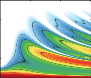
The simulations shown in figures 6–8 illustrate the importance of the intermediate stages of the DSW evolution. In both cases the initial perturbation evolves as a non-dispersive Riemann wave for approximately  $30$
$30$  $L$ (
$L$ ( $100$ km for the reference wave) for $\sigma ^{2}=795$, and approximately twice this distance for $\sigma ^{2}=397$. At approximately this point, solitons emerge ordered by their height, the tallest ones move faster. Despite the long integration domain, the complete disintegration predicted by the theory does not occur, much larger times are required. For the $\sigma ^{2}=397$ case only 4 solitons can be distinguished as truly separated, with perhaps two more beginning to form toward the end of the domain (figure 6a). Similarly, only 6 out of the expected 12 solitons may be confidently identified for the $\sigma ^{2}=795$ case (figure 7a).
Evolution of perturbation with  $\sigma ^{2}=397$ (reference wave amplitude 0.5 m). (a,d,g) Incoming wave; (b,e,h) transmitted wave; (c,f,i) reflected wave. (a–c) Upslope propagation, from 50 m to 1 m. (d–f) Downslope propagation from 50 m to 1000 m. (g–i) Modal variance normalized by the maximum value. The red box (g–i) indicates the spectral band subjected to strong reflection; the energy flux fraction outside the red box is <5 %. Time and space units are scaled by the characteristic scales $T$ and $L$ of the initial perturbation.

Same as in figure 6 but for a wave with  $\sigma ^{2}=795$ (reference wave amplitude 1.0 m).

Solitons identified in the numerical simulation with  $\sigma ^{2}=397$ (reference amplitude 0.5 m) at the end of the integration domain $600\ L$ (2000 km for the reference wave). Panel columns: incoming, transmitted and reflected waves. (a–c) Free surface elevation. (d–f) Modal variance. The reflected energy flux fraction outside the red box in the lower panels is less than 10 %.

The DSW is most effective in transferring energy away from the strong reflection band (figures 6–7g–i). As soon as solitons form they dominate the transmitted variance (variance outside the red box increases substantially, figures 6–7, panel h). Note that the shifting variance lobes are an artefact of the Fourier transform of the entire time series, which converts soliton separation into phase modulation. The modulation disappears if solitons are considered considered in isolation (figure 8d–f), however, because the disintegration is incomplete, only well-separated leading solitons can be confidently identified (figure 8a–c). Figure 9 compares the solitons identified in the solution after propagating for 600  $L$ (reference wave, $2000$ km), with the asymptotic solution ((3.6); Karpman Reference Karpman1967, Reference Karpman1975). While taller solitons are practically identical to the analytic form (also a validation of the numerical integration), lower solitons are not fully formed yet.
Numerical solitons (dots) compared with the analytical solution (lines, (3.6)) for  $\sigma ^{2}=397$ and $\sigma ^{2}=795$ (reference amplitudes 0.5 m and 1.0 m, expected to produce 8 and 12 solitons, respectively). Numerical solitons are identified at the end of the integration domain $600\ L$ (2000 km for the reference wave).

Because the first emerging solitons are taller and narrower, they are more effective in transferring energy to higher wavenumbers and high transmission rates; lagging solitons may have widths comparable to that of the initial perturbation and, therefore, experience a similarly strong reflection. Under the adopted idealization of flat bottom for the DSW evolution, the amplitudes and widths of the solitons eventually emerging out of any given initial perturbations can be easily found by employing the inverse scattering transform; for example, the amplitudes and hence widths of the solitons emerging out of sech-squared initial elevation (3.5) are given by explicit formulae (3.6).
However, to find out how many solitons would form for a given initial perturbation and distance to the toe of the slope one has to resort to numerical simulation. While the nature of the reflection process makes the slope opaque to long waves, the DSW disintegration breaks down the initial perturbation into ‘particles’ (solitons) carrying ‘quanta’ of energy flux (3.7). Smaller (narrower) particles carry larger quanta and have larger transmission rates. The slope can be transparent at least for some of the ‘particles’ resulting from the DSW disintegration.
The strength of the self-induced transparency effect is primarily controlled by the magnitude of the Ursell number  $\sigma ^{2}$. The nonlinearity, as quantified by $\sigma ^{2}$, affects the process in several ways:
(i) the DSW disintegration occurs earlier for larger $\sigma ^{2}$ (compare figures 6–7a–c);
(ii) the number of emerging solitons increases for larger
$\sigma ^{2}$ ((3.6); figures 6–7);(iii) the height of resulting solitons increases (3.6), which means that the energy carried by each soliton increases (3.7), and the emerging solitons are narrower (figure 9).
(iv) Overall, energy flux transmission increases. Figure 10 shows the evolution of the transmitted fraction of the total incoming energy flux for
$8\times 10^1\leq \sigma ^{2}\leq 1.2\times 10^2$ (reference wave: $0.1\leq a\leq 1.5$ m) for a distance of propagation of ${\approx }450\ L$ (reference wave, ${\approx }2000$ km). The transmitted fraction of total energy flux monotonically increases with $\sigma ^{2}$ and the degree of soliton separation. Over a flat bottom the process approaches saturation as the solitons approach the asymptotic state, but the distances required are not realistic. As noted before, the simple wave deformation prior to the gradient catastrophe accounts for only an approximately 3 % increase in transmission efficiency. For realistic bathymetries, only the first few solitons are likely to get fully separated. Hence reliance upon IST formulae might considerably overestimate the transmission.


Transmitted fraction of total energy flux for initial perturbation with  $80\leq \sigma ^{2}\leq 1200$ or for the reference wave with the amplitude $a$ in the range $0.1\leq a\leq 1.5$ m. Black lines represent the transmitted fraction for non-dispersive propagation. The lines in the detached ‘column’ to the right show the transmitted flux calculated by employing the asymptotic solution (3.6). The total propagation distance is ${\approx }600\ L$, or 2000 km for the reference wave.

5. Discussion
Here, we briefly discuss the sensitivity of the general picture to the underlying assumptions and approximations we adopted.
A key element of the broad picture is the high-pass filter behaviour of linear scattering by a localized inhomogeneity. Although analytical results supporting the high-pass filter role of bathymetry inhomogeneity exist only in the linear setting for a few geometrically simple inhomogeneity models (Meyer Reference Meyer1975, Reference Meyer1979; Mei et al. Reference Mei, Yue and Stiassnie2005; Ermakov & Stepanyants Reference Ermakov and Stepanyants2020), the behaviour of smaller scale harmonics can always be described using the WKB approximation, which suggests that this behaviour is universal within the linear theory framework, and may be extended to the weakly nonlinear waves. Indeed, for the bathymetry profile with an inhomogeneity of scale  $\varLambda$ (e.g. $L_{12}$ in figure 2b), estimating the ‘nonlinearity length’ as the distance to ‘gradient catastrophe’ yields ${L}/{\epsilon }$. The assumption that $\varLambda \ll {L}/{\epsilon }$ allows for neglecting, in the first order, the effect of the nonlinearity on the slope. This regime is applicable to a wide range of realistic situations. When this assumption is not valid, the self-induced transparency phenomenon does not disappear, it just becomes more complex and exhibits a new dynamics. For example, for high enough initial nonlinearity, pulses resulting from the ‘primary’ DSW disintegration could develop ‘secondary’ DSWs, further enhancing the phenomenon; or could become strongly nonlinear and break. In fact, a number of interesting scenarios may be imagined which merit dedicated studies. For example, if adiabatic evolution of the DSW solitons is plausible, the nonlinear Green's law (shoaling soliton's amplitude growing inversely proportional to local depth) could be applied. Moreover, although ignored here for the sake of simplicity, wave breaking deserves a dedicated investigation. While there is a wide range of non-breaking regimes of evolution, delineating breaking and non-breaking regimes in the parameter space goes beyond the scope of this work. Here, we just note that breaking obviously weakens the self-induced transparency effects.
Replacing the flat segments in out model bathymetry with mild sloping segments should ensure negligible reflection, and could enhance the DSW transfer of energy into smaller scales. The essence of the DSW self-induced transparency phenomenon will be preserved, but the governing equation will switch from the KdV form used here to a variable coefficient KdV. Qualitatively, for shoaling waves the number of solitons produced increases while their scale decreases, which has the effect that the transmitted fraction of the energy flux increases steadily instead of saturating as for the flat bathymetry case. We stress that, if reflection over the mildly sloping segment remains negligible, whatever is the bathymetry profile, the wave dynamic up to the reflecting part of the bathymetry could be studied using the variable coefficient KdV equation without much additional numerical effort.
These arguments suggest that the key elements of the mechanism, the inhomogeneity high-pass filter and DSW disintegration, are robust and not sensitive to tweaking either the model or topography. Moreover, even if we take into consideration the factors and effects a priori neglected, such as the three-dimensional bathymetry and wave fields, bottom friction and interaction with the atmosphere, we do not see a candidate mechanism potentially able to destroy the phenomenon.
Although the calculations presented in the paper demonstrate the relevance of the self-induced transparency for long ocean waves, the model is too simplified for realistic tsunami/meteotsunami applications. Although we argued that the phenomenon is universal, we stress that its manifestation is specific for each bathymetry. Quantifying the DSW disintegration for any given conditions requires extensive direct integration of the Boussinesq equations for the specific bathymetry and a range of parameters of incoming waves. For long ocean waves, numerical models are readily accessible (e.g. FUNWAVE-TVD Shi et al. (Reference Shi, Kirby, Tehranirad, Harris, Choi and Malej2016), tested and validated over many years), but this task goes beyond the scope of present work.
We conclude this discussion by noting that the elements of the self-induced transparency mechanism are robust, universal physical processes, which implies that the phenomenon itself is universal and robust. The Boussinesq-type equations with inhomogeneity play a fundamental role in many physical contexts, such as e.g. long internal gravity waves (e.g. Grimshaw et al. Reference Grimshaw, Ostrovsky, Shrira and Stepanyants1998), plasmas (Karpman Reference Karpman1975) and nonlinear waves in solids (Khusnutdinova, Gavrilyuk & Ostrovsky Reference Khusnutdinova, Gavrilyuk and Ostrovsky2023). Scattering by localized homogeneities is also a universal phenomenon, and its high-pass filter behaviour is well documented in the framework of linear theory (e.g. Felsen & Marcuwitz Reference Felsen and Marcuwitz1994; Lekner Reference Lekner2016).
While DSW structures associated with tsunami/meteotsunami waves provided a major motivation for this study, it should be noted that they are rare occurrences in comparison with the daily occurring internal tide DSWs formed by propagation on the continental shelf (e.g. Vlasenko, Stashchuk & Hutter Reference Vlasenko, Stashchuk and Hutter2005). Predicting the amount of energy brought into the shelf area by each tidal cycle is important for estimating shelf ‘ventilation’ and its impact on shelf biological processes. The dynamics of long internal waves on the shelf is governed by the same Boussinesq equations modified to account for the Earth's rotation with the stratification profiles incorporated into the coefficients (e.g. Grimshaw et al. Reference Grimshaw, Ostrovsky, Shrira and Stepanyants1998).
Furthermore, we expect the DSW self-induced transparency mechanism to be far more general than the Boussinesq-type equations with inhomogeneity and to be applicable to a wide class of weakly dispersive systems. In particular, we have not touched on possible effects due to higher-order nonlinear terms; the conclusions we arrived at are expected to stand for the Euler equations without any simplifications. These expectations remain to be properly developed and verified.
6. Conclusion
The main result of this study is introducing and elucidating the long wave DSW self-induced transparency as a mechanism affecting the reflection/transmission of the wave at a bathymetric inhomogeneity. The idealized bathymetric profile used here allows for separating the effects of nonlinearity and dispersion from those of the reflection at a bathymetric inhomogeneity which, in turn, elucidates their roles in the phenomenon of long wave self-induced transparency. Although the quantitative analysis presented here is limited to this idealized bathymetry, its results outline a general picture of the phenomenon and allows for qualitative predictions for other bathymetry profiles. Thus, we conclude that the DSW self-induced transparency is a universal phenomenon. However, its manifestation in realistic conditions is expected to depend strongly on the specific bathymetry and initial wave parameters. For these applications, quantitative predictions may be obtained only using numerical simulation using numerical models of matching complexity.
Within the wide range of parameters we examined, the DSW disintegration is shown to be effective in transferring energy flux across the scale boundary that separates the high and low reflection domains in the parameter space. As a result, the self-induced transparency can be an order-one effect: reflection can drop from order one to nearly zero. The mechanism works both for up- and downslope bathymetric inhomogeneities. The generation of bound harmonics, dominant for non-dispersive waves, has a much weaker effect, up to 3.5 %, on reflection/transmission.
Funding
The work was supported by NSFGEO-NERC program, NSF grant no. 1737274 and NERC grant NE/R012202. V.I.S. is grateful to the Isaac Newton Institute for Mathematical Sciences, Cambridge, for support and hospitality during the stimulating programme ‘Dispersive hydrodynamics: mathematics, simulation and experiments, with applications in nonlinear waves’ supported by EPSRC grant EP/R014604/1; the work in this paper was partially undertaken by V.I.S. at INI.
Declaration of interests
The authors report no conflict of interest.
Appendix. Numerical testing of the decoupling hypothesis
A fundamental hypothesis we employed in this study is that, if the sloping transition between two shelves is steep enough and the incoming perturbation is localized, the evolution of the incoming and reflected waves is effectively decoupled. To leading order, the nonlinear interaction between the incoming and reflected waves may be neglected, and wave reflection in the chosen regime is approximately linear. This assumption greatly simplifies the problem by reducing the problem of dealing with counter-propagating waves (e.g. Boussinesq equation) to the two independent parts: unidirectional propagation (KdV equation) for the incoming wave, and an ‘offline’ linear calculation of reflected and transmitted waves. We stress that the hypothesis is needed only for the simplification of the consideration.
The nonlinear interaction between two counter-propagating pulses was thoroughly studied by Khusnutdinova & Moore (Reference Khusnutdinova and Moore2012) and Khusnutdinova, Moore & Pelinovsky (Reference Khusnutdinova, Moore and Pelinovsky2014) from a different perspective. We are not aware of dedicated studies of the nonlinear interaction of two counter-propagating waves in the Boussinesq-type equations with inhomogeneity, but have every reason to expect that the same logic as in the homogeneous case should be applicable. This assumption could be verified by direct integration of the Boussinesq equations. Here, we test the plausibility of this hypothesis by comparing the simple KdV/linear reflection representation used in this study with numerical results of a numerical Boussinesq model. To this end we use the FUNWAVE-TVD model, which is the official shallow water model of the US Army Corps of Engineers, and has a long list of well-tested capabilities (Kirby et al. Reference Kirby, Wei, Chen, Kennedy and Dalrymple1998; Shi et al. Reference Shi, Kirby, Harris, Geiman and Grilli2012a; Shi, Kirby & Tehranirad Reference Shi, Kirby and Tehranirad2012b; Kirby et al. Reference Kirby, Shi, Tehranirad, Harris and Grilli2013; Malej, Smith & Salgado-Dominguez Reference Malej, Smith and Salgado-Dominguez2015; Kirby Reference Kirby2016; Shi et al. Reference Shi, Kirby, Tehranirad, Harris, Choi and Malej2016, Reference Shi, Malej, Smith and Kirby2018).
Before attempting such a comparison, however, some precautions have to be made. The KdV/linear reflection representation adopted here was formulated to retain the minimal set of processes essential to the self-induced transparency phenomenon: balanced nonlinearity and dispersion, and reflection. All other processes were purposely ignored. In contrast, FUNWAVE-TVD is a numerical framework built for the opposite goal – to include all the processes relevant for shallow water wave evolution. Bringing the two models to some level of capability parity would require either adding extra physics to our simple model, or stripping FUNWAVE-TVD of some of its capabilities. Neither proposition fits into the scope of this study. The only alternative is to reformulate the problem in a way that may be simulated in FUNWAVE-TVD by engaging a minimal subset of physics.
For the comparison, we use the settings of the chosen reference wave: an initial positive perturbation of the sech-squared form (3.5) with amplitude 0.8 m, width  $L\approx 3.3$ km and time scale $T=150$ s ( $\sigma ^{2}=636$), propagating over a shelf of $h_{2}=50$ m depth toward a slope of 0.015. To avoid engaging FUNWAVE-TVD wave breaking modules over the slope, the shallow shelf was set at $h_{1}=10$ m. The propagation on the 50 m depth shelf was simulated for 1000 km at a 20 m grid step, and then the output was used as a hot start for a secondary higher resolution (0.75 m grid step) run over the slope.
Figure 11 compares the FUNWAVE-TVD results with the KdV/reflection model used here for the propagation distances of 320, 440, 560, 1040 km. The results agree well in both shape and magnitude of the reflected wave, considering that the FUNWAVE-TVD runs exhibit a significant energy loss: 0.02, 0.06, 0.09 and 0.2 for the four distances, respectively. This suggests that the decoupling hypothesis works well in the highly idealized framework of the KdV/linear reflection model.
Comparison between FUNWAVE-TVD and currently adopted KdV/linear reflection mode for the reference wave with an amplitude of 0.8 m,  $\sigma ^{2}=636$. (a–d) Incoming DSW structure at the slope toe. (e–h) Reflected wave. To avoid the breaking regime, the shallow shelf is set here at $h_{2}=10$ m.


 Open access