


1 Introduction
Turbulent convection is a commonly occurring phenomenon in the oceans and atmosphere. Deep convection in open ocean is a particular form of turbulent convection observed especially at high latitudes, such as the Northwestern Mediterranean, the Labrador Sea, the Central Greenland Sea and the Weddell Sea. The surface waters at these locations become denser, either due to atmospheric cooling or brine rejection, and sink to greater depths. Deep-ocean convection plays an important role in thermohaline circulation (Marshall & Schott Reference Marshall and Schott1999) through an efficient vertical mixing process which sometimes results in well-mixed layers extending down to the abyss. The review article by Killworth (Reference Killworth1983) provides useful insights into the mechanism of open-ocean convection at various locations around the globe. However, advances in observational techniques, sophisticated experimental tools and numerical modelling have improved our understanding of the dynamics of deep-ocean convection as reviewed by Marshall & Schott (Reference Marshall and Schott1999).
The first attempt to unravel the mysteries of open-ocean deep convection is the classical Mediterranean Ocean Convection (MEDOC) experiment in the Gulf of Lions, Northwestern Mediterranean (Medoc Reference Medoc1970). The MEDOC experiment demonstrated the formation of a homogeneous region as a consequence of surface forcing by strong cold winds. Mixing of the water column down to 2000 m within a few days was observed. Further investigations carried out by Gascard (Reference Gascard1978) and Leaman & Schott (Reference Leaman and Schott1991) demonstrated the regular occurrence of deep convection at the end of the winter period in the Gulf of Lions. The experiments of Leaman & Schott (Reference Leaman and Schott1991) and Schott et al. (Reference Schott, Visbeck, Send, Fischer, Stramma and Desaubies1996) depicted the existence of small-scale convection cells, known as plumes, in the Gulf of Lions and deduced that these plumes behave as mixing agents rather than transporting bulk fluid in the downward direction. Analogous experiments by Schott, Visbeck & Fischer (Reference Schott, Visbeck and Fischer1993) in the Greenland Sea also corroborated the presence of plumes and their role as mixing agents. More recently, observations by Testor et al. (Reference Testor, Bosse, Houpert, Margirier, Mortier, Legoff, Dausse, Labaste, Karstensen and Hayes2018) in the Northwestern Mediterranean Sea reported deepening of the mixed layer owing to horizontal inhomogeneities in density. They also observed sharpening of fronts and the development of baroclinic instabilities resulting in mesoscale turbulence. Similarly, field experiments were also conducted in the Labrador Sea by Lazier (Reference Lazier1973) and Clarke & Gascard (Reference Clarke and Gascard1983), and the presence of deep, mixed water columns as a result of inter-annual variation in temperature and salinity was reported. Gordon (Reference Gordon1982) have also documented the sinking of freezing point surface water to a depth of approximately 2700 m in the Weddell Sea during the winter.
Laboratory experiments of localized convection are also conducted by either imposing a source of buoyancy flux at the surface (Maxworthy & Narimousa Reference Maxworthy and Narimousa1994; Whitehead, Marshall & Hufford Reference Whitehead, Marshall and Hufford1996) or by heating the bottom boundary (Brickman Reference Brickman1995; Coates, Ivey & Taylor Reference Coates, Ivey and Taylor1995; Ivey, Taylor & Coates Reference Ivey, Taylor and Coates1995) in a rotating environment. The experiments of Maxworthy & Narimousa (Reference Maxworthy and Narimousa1994) were performed in an unstratified medium, and agree with the findings of Jones & Marshall (Reference Jones and Marshall1993), especially in terms of the length and velocity scales of the plumes. Similar plumes are also reported by Aurnou et al. (Reference Aurnou, Andreadis, Zhu and Olson2003) in their thermal convection experiments in a rotating fluid. Whitehead et al. (Reference Whitehead, Marshall and Hufford1996), however, carried out their experiments in a stratified medium and concluded that the depth of penetration of the convective mixed layer depends only on the nature of the surface buoyancy flux and ambient stratification rather than rotation. The unstratified experiments of Brickman (Reference Brickman1995) and the stratified experiments of Ivey et al. (Reference Ivey, Taylor and Coates1995) and Coates et al. (Reference Coates, Ivey and Taylor1995) revealed the formation of baroclinic eddies at the edges of the heating disk after the initial evolution, and are responsible for the lateral distribution of heat. Recently, Frank et al. (Reference Frank, Landel, Dalziel and Linden2017) conducted experiments on saltwater point plumes in an unstratified rotating environment and highlighted the importance of background rotation in the evolution of plumes. They reported anticyclonic precession of the plume at a rate proportional to the background rotation rate.
Several numerical studies were also performed (Madec et al. Reference Madec, Delecluse, Crepon and Chartier1991; Jones & Marshall Reference Jones and Marshall1993; Denbo & Skyllingstad Reference Denbo and Skyllingstad1996; Legg, McWilliams & Gao Reference Legg, McWilliams and Gao1998; Raasch & Etling Reference Raasch and Etling1998; Noh, Jang & Kim Reference Noh, Jang and Kim1999; Noh, Cheon & Raasch Reference Noh, Cheon and Raasch2003) with a focus on understanding the flow physics and quantifying the length and velocity scales of the plumes in deep-ocean convection. The subgrid-scale features in these simulations were parameterized by using either eddy viscosity models or a high artificial viscosity and, therefore, the small-scale turbulence was not explicitly resolved. The simulations of Madec et al. (Reference Madec, Delecluse, Crepon and Chartier1991), with the help of a simple parameterization scheme of convection, focused on the mechanism responsible for the generation of the mesoscale features and the energetics associated with them in deep-ocean convection in the Northwestern Mediterranean Sea. Jones & Marshall (Reference Jones and Marshall1993) performed simulations of localized convection in a neutral environment using a non-hydrostatic ocean model and proposed length and velocity scaling of the plumes. They deduced that if the dynamics of the deep-ocean convection is dominated by the Earth’s rotation, the length and velocity of the plumes vary as  $(B_{0}/f^{3})^{1/2}$ and $(B_{0}/f)^{1/2}$ respectively. However, if the rotational effects are weak and the ocean depth becomes important, the length and velocity scale as $L_{3}$ (fluid depth) and $(B_{0}L_{3})^{1/3}$, respectively. Large eddy simulations (LES) were performed by Raasch & Etling (Reference Raasch and Etling1998) to investigate the growth of the convective mixed layer as a consequence of localized heating at the bottom boundary in a rotating and stably stratified fluid. The heating flux magnitude considered in their study was four orders of magnitude larger compared to the typical cooling flux magnitudes measured in the ocean. Noh et al. (Reference Noh, Jang and Kim1999) also carried out LES to study the effects of preconditioning and surface flux magnitude on convective patterns. Direct numerical simulations were performed by Julien et al. (Reference Julien, Legg, McWilliams and Werne1996a,Reference Julien, Legg, McWilliams and Werneb) to study the dynamics of plumes and the energetics in Rayleigh–Bénard convection under the influence of rapid rotation.
In this study, localized convection typically observed in open-ocean deep convection is considered. The current problem set-up is different from the classical ‘Rayleigh–Bénard’ convection (Bénard Reference Bénard1901; Rayleigh Reference Rayleigh1916). The convective processes in the ocean are characterized by intermittent localized forcing (Gascard & Clarke Reference Gascard and Clarke1983) at the surface whereas the Rayleigh–Bénard convection typically represents the convective phenomenon between two infinite plates at different temperatures. Although the initial evolution for both deep-ocean convection and Rayleigh–Bénard convection have similar characteristics such as plume formation, the late time flow evolution in deep-ocean convection is significantly influenced by the horizontal inhomogeneities in density, resulting in an entirely different set of physical processes such as baroclinic instabilities and slantwise convection. The formation of a rim current at the interface of the mixed and surrounding fluid is also a distinctive feature found in the deep-ocean convection and is absent in traditional Rayleigh–Bénard convection.
Deep-ocean convection has traditionally been categorized into three phases (Medoc Reference Medoc1970; Jones & Marshall Reference Jones and Marshall1993; Marshall & Schott Reference Marshall and Schott1999) namely pre-conditioning, violent mixing and sinking and spreading. The pre-conditioning phase sets up an environment for the convection process by transporting weakly stratified fluid from the interior of the ocean to the surface by means of large-scale cyclonic circulations. Legg et al. (Reference Legg, McWilliams and Gao1998) and Noh et al. (Reference Noh, Cheon and Raasch2003) investigated the influence of pre-conditioning on the dynamics of the deep-ocean convection in a stratified environment by imposing uniform surface buoyancy loss and mesoscale eddies as initial conditions. In the studies with disk-shaped surface cooling, the location of the deep convection remains fixed whereas the presence of an initial mesoscale eddy gives deep convection the liberty of evolving in response to the motion of the baroclinic eddies and changes in stratification. The cooling at the surface instigates the violent-mixing phase during which the denser fluid at the surface sinks to greater depths in the form of multiple plume-like structures, resulting in overturning and mixing of the entire water column. This localized mixing results in lateral density gradients between the mixed fluid and the surrounding fluid. The sinking and spreading phase begins with the weakening of the surface cooling, as a consequence of which the convective overturning process ceases. The lateral density front under the influence of rotation undergoes baroclinic instabilities and results in baroclinic eddies responsible for lateral mixing, entrainment of surrounding fluid and restratification of the water column.
Although different phases of deep-ocean convection and their roles in overall large-scale circulation are studied extensively (Medoc Reference Medoc1970; Jones & Marshall Reference Jones and Marshall1993; Marshall & Schott Reference Marshall and Schott1999), there are discrepancies in the parameterization of deep-ocean convection due to the poor representation of small-scale turbulence. The vertical mixing during convection occurs over hundreds of metres during a period of hours (Aagaard & Carmack Reference Aagaard and Carmack1989). The existing ocean general circulation models (OGCMs) cannot resolve these convective processes owing to their coarse resolution. Therefore, the OGCMs use one-dimensional (1-D) parameterization schemes (Rahmstorf Reference Rahmstorf1993; Klinger, Marshall & Send Reference Klinger, Marshall and Send1996; Paluszkiewicz & Romea Reference Paluszkiewicz and Romea1997) to represent the convective processes. These parameterizations inherently assume homogeneity in the horizontal directions. In the real ocean the mixing owing to convection is heterogeneous in nature (M. Ilicak, Adcroft & Legg Reference Ilicak, Adcroft and Legg2014). Therefore, these 1-D parameterization schemes are unable to accurately model the effect of small-scale turbulence on large-scale circulation. In this study, we perform direct numerical simulations (DNS) and LES with a focus on small-scale turbulence in the deep-ocean convection process, particularly during the violent-mixing phase. The present simulations explicitly resolve the energy containing eddies of the flow imperative for understanding the effect of small-scale turbulence on the evolution of large-scale flow structures. Note that DNS are carried out in a scaled-down computational box and LES are performed at large scales  $O$(10 km) while keeping the Rossby number for both DNS and LES relevant to realistic values observed in the ocean. We explore if the scaling laws proposed by Jones & Marshall (Reference Jones and Marshall1993) under neutral ocean conditions are valid in a weakly stratified environment with Brunt–Väisälä frequency $N\leqslant f$. We also investigate the effects of rotation on the overall flow evolution by varying the background rotation rate.
The problem formulation is presented in § 2. Results from the numerical simulations are discussed in § 3 and the conclusions drawn from this study are given in § 4.
2 Problem formulation
2.1 Governing equations
The three-dimensional conservation equations for mass, momentum and temperature deviation from the background subject to the Boussinesq approximation for an unsteady incompressible flow are
continuity:
 $$\begin{eqnarray}\unicode[STIX]{x1D735}\boldsymbol{\cdot }\boldsymbol{u}=0,\end{eqnarray}$$
momentum:
 $$\begin{eqnarray}\frac{\unicode[STIX]{x2202}\boldsymbol{u}}{\unicode[STIX]{x2202}t}+\boldsymbol{u}\boldsymbol{\cdot }\unicode[STIX]{x1D735}\boldsymbol{u}=-\frac{1}{\unicode[STIX]{x1D70C}_{0}}\unicode[STIX]{x1D735}p^{\prime }-f\hat{\boldsymbol{k}}\times \boldsymbol{u}-\frac{\widetilde{\unicode[STIX]{x1D70C}}}{\unicode[STIX]{x1D70C}_{0}}g\hat{\boldsymbol{k}}+\unicode[STIX]{x1D708}\unicode[STIX]{x1D6FB}^{2}\boldsymbol{u}-\unicode[STIX]{x1D735}\boldsymbol{\cdot }\unicode[STIX]{x1D749},\end{eqnarray}$$
temperature:
 $$\begin{eqnarray}\frac{\unicode[STIX]{x2202}\widetilde{T}}{\unicode[STIX]{x2202}t}+\boldsymbol{u}\boldsymbol{\cdot }\unicode[STIX]{x1D735}\widetilde{T}=\unicode[STIX]{x1D705}_{t}\unicode[STIX]{x1D6FB}^{2}\widetilde{T}-u_{3}\frac{\unicode[STIX]{x2202}\overline{T}(x_{3})}{\unicode[STIX]{x2202}x_{3}}-\unicode[STIX]{x1D735}\boldsymbol{\cdot }\unicode[STIX]{x1D740}+F_{T}.\end{eqnarray}$$
 Here,  $\boldsymbol{u}$ is the velocity vector with components ( $u_{1},u_{2},u_{3}$) in the $x_{1}$, $x_{2}$ and $x_{3}$ (vertical) directions respectively, $p^{\prime }$ is the deviation of pressure from the hydrostatic background state, $f$ is the Coriolis parameter, $g=9.81~\text{m}~\text{s}^{-2}$ is the acceleration due to gravity, $\unicode[STIX]{x1D708}\;(\text{m}^{2}~\text{s}^{-1})$ is the kinematic viscosity, $\unicode[STIX]{x1D705}_{t}\;(\text{m}^{2}~\text{s}^{-1})$ is the thermal diffusivity and the Prandtl number $Pr=\unicode[STIX]{x1D708}/\unicode[STIX]{x1D705}_{t}$. The terms $\unicode[STIX]{x1D749}$ and $\unicode[STIX]{x1D740}$ represent the subgrid stress tensor and temperature flux vector respectively. In the case of DNS, these terms will be zeros as all the scales of the flow are well resolved and there is no need for any subgrid-scale parameterization. However, in the case of LES, these terms need to be evaluated from the resolved components of the velocity and temperature fields. The subgrid-scale stress, $\unicode[STIX]{x1D70F}_{ij}$, and subgrid temperature flux, $\unicode[STIX]{x1D706}_{j}$, are parameterized as follows:
 $$\begin{eqnarray}\displaystyle & \displaystyle \unicode[STIX]{x1D70F}_{ij}=-2C_{d}\widehat{\unicode[STIX]{x1D6E5}}^{2}|\unicode[STIX]{x1D64E}|\widehat{\unicode[STIX]{x1D61A}_{ij}}, & \displaystyle\end{eqnarray}$$
 $$\begin{eqnarray}\displaystyle & \displaystyle \unicode[STIX]{x1D706}_{j}=-C_{\unicode[STIX]{x1D703}}\widehat{\unicode[STIX]{x1D6E5}}^{2}|\unicode[STIX]{x1D64E}|\frac{\unicode[STIX]{x2202}\widehat{T}}{\unicode[STIX]{x2202}x_{j}}, & \displaystyle\end{eqnarray}$$
 where  $\widehat{\unicode[STIX]{x1D6E5}}$ is the filter (top hat) width, $C_{d}$ is the model coefficient, $\widehat{\unicode[STIX]{x1D61A}}_{ij}=1/2(\unicode[STIX]{x2202}\widehat{u}_{i}/\unicode[STIX]{x2202}x_{j}+\unicode[STIX]{x2202}\widehat{u}_{j}/\unicode[STIX]{x2202}x_{i})$ is the resolved strain rate and $|\unicode[STIX]{x1D64E}|$ is defined as $\sqrt{2\widehat{\unicode[STIX]{x1D61A}}_{ij}\widehat{\unicode[STIX]{x1D61A}}_{ij}}$. The subgrid eddy viscosity and diffusivity are computed using the Smagorinsky model as:
 $$\begin{eqnarray}\displaystyle & \displaystyle \unicode[STIX]{x1D708}_{sgs}=C_{d}\widehat{\unicode[STIX]{x1D6E5}}^{2}|\unicode[STIX]{x1D64E}|, & \displaystyle\end{eqnarray}$$
 $$\begin{eqnarray}\displaystyle & \displaystyle \unicode[STIX]{x1D705}_{sgs}=C_{\unicode[STIX]{x1D703}}\widehat{\unicode[STIX]{x1D6E5}}^{2}|\unicode[STIX]{x1D64E}|, & \displaystyle\end{eqnarray}$$
 respectively. The model coefficient  $C_{d}$ is taken as 0.17 (Lilly Reference Lilly1967; McMillan & Ferziger Reference McMillan and Ferziger1979; Meyers & Sagaut Reference Meyers and Sagaut2006) and, since the turbulent Prandtl number ( $Pr_{t}$) is assumed to be 1 (Taylor & Ferrari Reference Taylor and Ferrari2010), $C_{\unicode[STIX]{x1D703}}$ is also taken as 0.17.
The temperature can be decomposed into a reference temperature,  $T_{0}$, background variation in the $x_{3}$ direction, $\overline{T}(x_{3})$, and a deviation from the background, $\tilde{T}(x_{i},t)$, given by
 $$\begin{eqnarray}T=T_{0}+\overline{T}(x_{3})+\widetilde{T}(x_{i},t).\end{eqnarray}$$
 In the ocean, the density can change as a result of variations in temperature, salinity and pressure. However, in this study, since our focus is on understanding the plume scaling and turbulent dynamics for a given background condition, we assume the density to be a linear function of temperature only to avoid additional complexities. The density is given by  $\unicode[STIX]{x1D70C}=\unicode[STIX]{x1D70C}_{0}(1-\unicode[STIX]{x1D6FC}(T-T_{0}))$, where $T_{0}=298~\text{K}$ is the reference temperature, $\unicode[STIX]{x1D6FC}=2\times 10^{-4}~\text{K}^{-1}$ is the coefficient of thermal expansion of water and $\unicode[STIX]{x1D70C}_{0}=1000~\text{kg}~\text{m}^{-3}$ is the reference density. The density deviation and the temperature deviation are related to each other as follows:
 $$\begin{eqnarray}\widetilde{\unicode[STIX]{x1D70C}}(x_{i},t)=-\unicode[STIX]{x1D70C}_{0}\unicode[STIX]{x1D6FC}\widetilde{T}(x_{i},t).\end{eqnarray}$$
 The background temperature gradient is related to the Brunt–Väisälä frequency as  $\unicode[STIX]{x2202}\overline{T}(x_{3})/\unicode[STIX]{x2202}x_{3}=(1/g\unicode[STIX]{x1D6FC})N^{2}$. We have chosen a constant value for the Brunt–Väisälä frequency, $N=10^{-2}~\text{rad}~\text{s}^{-1}$ for DNS, and $N=3.16\times 10^{-5}~\text{rad}~\text{s}^{-1}$ for LES. The reason for such a selection is to keep the ratio $N/f\leqslant 1$ for DNS and LES. At the initial time, $t=0$, the temperature deviation is taken as zero. A surface forcing, $F_{T}$, is imposed at the top boundary in a circular region (see figure 1) given by $F_{T}=H/\unicode[STIX]{x1D70C}_{0}C_{w}h$, where $H=-800~\text{W}~\text{m}^{-2}$ is the cooling flux at the top surface, $C_{w}=3900~\text{J}~\text{Kg}^{-1}~\text{K}^{-1}$ is the specific heat of water and $h$ is the depth over which the surface forcing $F_{T}$ is applied. In our simulations, we apply the forcing at the first vertical grid cell i.e. $h=\unicode[STIX]{x0394}x_{3}$. Note that the buoyancy flux through the surface is related to the cooling flux by $B_{0}=g\unicode[STIX]{x1D6FC}H/\unicode[STIX]{x1D70C}_{0}C_{w}$ (Jones & Marshall Reference Jones and Marshall1993).
All the numerical values for the variables that will be discussed in the subsequent sections are in SI units ( $L_{1}$, $L_{2}$, $L_{3}$ are in metres, time $t$ is in seconds).

Figure 1. Schematic of the computational domain. The dimensions of the computational box are  $L_{1},L_{2}$ and $L_{3}$ respectively in the $x_{1},x_{2}$ and $x_{3}$ directions. The coordinates of the computational domain are in the ranges $(-L_{1}/2,L_{1}/2)$, $(-L_{2}/2,L_{2}/2)$ and $(-L_{3},0)$ respectively. The surface forcing is applied in a circular region of radius $r_{0}=0.114L_{1}$ centred at $(0,0,0)$ for both DNS and LES cases. All of the dimensional and non-dimensional parameters are given in tables 1 and 2.
Table 1. Simulation parameters for DNS: here  $B_{0}$ is the magnitude of the buoyancy flux applied near the surface, $f$ is the Coriolis parameter. $Ra_{f}=B_{0}L_{3}^{4}/\unicode[STIX]{x1D705}_{t}^{2}\unicode[STIX]{x1D708}$ is the (flux) Rayleigh number, where $\unicode[STIX]{x1D705}_{t}=0.143\times 10^{-6}~\text{m}^{2}~\text{s}^{-1}$ is the thermal diffusivity and $\unicode[STIX]{x1D708}=10^{-6}~\text{m}^{2}~\text{s}^{-1}$ is the kinematic viscosity. The Rossby number is defined as $Ro=B_{0}^{1/2}/f^{3/2}L_{3}$. The number of grid points used for all of the cases in the $x_{1}$, $x_{2}$ and $x_{3}$ directions are $N_{x}=1024$, $N_{y}=1024$ and $N_{z}=512$ respectively. The domain lengths in the corresponding directions are $L_{1}=2.2~\text{m}$, $L_{2}=2.2~\text{m}$ and $L_{3}=0.4~\text{m}$ for all of the cases listed above. $\mathscr{T}=2\unicode[STIX]{x03C0}/f$ is the inertial time period and signifies the importance of rotational effects on the flow.

2.2 Numerical method and simulation parameters
Equations (2.1)–(2.3) are discretized using a staggered-grid method, i.e. velocity fields are stored on the cell faces, whereas pressure and temperature fluctuations are stored at the cell centres. The governing equations are advanced in time using a mixed third-order Runge–Kutta and Crank–Nicolson scheme (Pham, Sarkar & Brucker Reference Pham, Sarkar and Brucker2009; Brucker & Sarkar Reference Brucker and Sarkar2010; Pal, de Stadler & Sarkar Reference Pal, de Stadler and Sarkar2013; Pham & Sarkar Reference Pham and Sarkar2014, Reference Pham and Sarkar2018; Pal & Sarkar Reference Pal and Sarkar2015). A second-order central finite-difference method is used to compute spatial derivatives. The dynamic pressure is obtained by solving the Poisson equation via a multigrid iterative method. Periodic boundary conditions are used in  $x_{1}$ and $x_{2}$ directions for all variables. In the vertical direction, Dirichlet and Neumann boundary conditions are used as follows:
 $$\begin{eqnarray}\frac{\unicode[STIX]{x2202}u_{1}}{\unicode[STIX]{x2202}x_{3}}(x_{3}=0,-L_{3})=0,\quad \frac{\unicode[STIX]{x2202}u_{2}}{\unicode[STIX]{x2202}x_{3}}(x_{3}=0,-L_{3})=0,\quad u_{3}(x_{3}=0,-L_{3})=0,\end{eqnarray}$$
 $$\begin{eqnarray}\frac{\unicode[STIX]{x2202}p^{\prime }}{\unicode[STIX]{x2202}x_{3}}(x_{3}=0,-L_{3})=0,\quad \frac{\unicode[STIX]{x2202}\widetilde{T}}{\unicode[STIX]{x2202}x_{3}}(x_{3}=0,-L_{3})=0.\end{eqnarray}$$
This solver has been extensively validated and used for several DNS (Pham et al. Reference Pham, Sarkar and Brucker2009; Brucker & Sarkar Reference Brucker and Sarkar2010; Pal et al. Reference Pal, de Stadler and Sarkar2013; Pal & Sarkar Reference Pal and Sarkar2015) and LES (Pham & Sarkar Reference Pham and Sarkar2014, Reference Pham and Sarkar2018) studies of stratified turbulence. Grid resolution in this study has been chosen such that the smallest scales of the flow (Kolmogorov scales) are well resolved in DNS.
Table 2. Simulation parameters for LES:  $\unicode[STIX]{x1D705}_{t}=1.2\times 10^{-2}~\text{m}^{2}~\text{s}^{-1}$ and $\unicode[STIX]{x1D708}=8.5\times 10^{-2}~\text{m}^{2}~\text{s}^{-1}$ for LES. The number of grid points used for all of the LES cases in the $x_{1}$, $x_{2}$ and $x_{3}$ directions are $N_{x}=768$, $N_{y}=768$ and $N_{z}=256$ respectively. The domain lengths in the respective directions are $L_{1}=11\,000~\text{m}$, $L_{2}=11\,000~\text{m}$ and $L_{3}=2000~\text{m}$ for all of the LES cases listed above.

The Reynolds decomposition of any of the following quantities  $u_{1}$, $u_{2}$, $u_{3}$ and $\widetilde{T}$ into mean and fluctuating components is given by
 $$\begin{eqnarray}\unicode[STIX]{x1D719}=\langle \unicode[STIX]{x1D719}\rangle +\unicode[STIX]{x1D719}^{\prime }.\end{eqnarray}$$
 Periodic boundary conditions are applied in the  $x_{1}$ and $x_{2}$ directions, and therefore horizontal averaging of the variables is performed to calculate the Reynolds averaged value as follows:
 $$\begin{eqnarray}\langle \unicode[STIX]{x1D719}\rangle ={\displaystyle \frac{1}{L_{1}\times L_{2}}}\int _{-L_{1/2}}^{L_{1/2}}\int _{-L_{2/2}}^{L_{2/2}}\unicode[STIX]{x1D719}\,\text{d}x_{1}\,\text{d}x_{2}.\end{eqnarray}$$
Figure 2. Contour plots of vertical velocity in the  $x_{2}=0$ plane for (a) $B_{0}=4\times 10^{-9}~\text{m}^{2}~\text{s}^{-3}$ (DNS1), (b) $B_{0}=4\times 10^{-8}~\text{m}^{2}~\text{s}^{-3}$ (DNS3) and (c) $B_{0}=4\times 10^{-7}~\text{m}^{2}~\text{s}^{-3}$ (DNS7). The domain height and Rossby number in all of these cases are $L_{3}=0.4~\text{m}$ and $Ro=0.32$, respectively. We have only shown the vertical domain in the range $[0,-0.25]$ in order to zoom in on the initial evolution of the plumes. Each snapshot corresponds to a time $t\approx 100\times (\unicode[STIX]{x1D705}_{t}/B_{0})^{1/2}$ for all three cases.
Tables 1 and 2 show the complete list of numerical experiments that we performed in this study. In the first set of test cases, corresponding to DNS (see cases DNS1–DNS7), the buoyancy flux magnitude and the Coriolis parameter are varied, keeping the Rossby number constant. We are motivated to quantify the initial plume characteristics such as plume velocity and diameter in terms of  $B_{0}$ and $\unicode[STIX]{x1D705}_{t}$. The number of grid points in all of the DNS cases is $N_{x}=1024$, $N_{y}=1024$ and $N_{z}=512$ in the $x_{1}$, $x_{2}$ and $x_{3}$ directions, respectively. The corresponding domain lengths are $L_{1}=2.2~\text{m}$, $L_{2}=2.2~\text{m}$ and $L_{3}=0.4~\text{m}$. Similarly, we have performed additional large eddy simulations (see table 2, cases LES1–LES6) to verify if the scaling obtained from the DNS simulations performed at laboratory scale is still valid at geophysical scales. The number of grid points in all of the LES cases in the $x_{1}$, $x_{2}$ and $x_{3}$ directions is $N_{x}=768$, $N_{y}=768$ and $N_{z}=256$ respectively. The domain lengths in the respective directions are $L_{1}=11\,000~\text{m}$, $L_{2}=11\,000~\text{m}$ and $L_{3}=2000~\text{m}$. Also, it is to be noted that, in the LES cases, the thermal diffusivity $\unicode[STIX]{x1D705}_{t}=1.2\times 10^{-2}~\text{m}^{2}~\text{s}^{-1}$, and kinematic viscosity $\unicode[STIX]{x1D708}=8.5\times 10^{-2}~\text{m}^{2}~\text{s}^{-1}$, so as to keep the flux Rayleigh number similar between the DNS and LES cases. All of the results in the upcoming sections are presented in dimensional time units.
3 Results
3.1 Initial evolution
Cooling at the surface increases the density of the fluid in the top layers. Therefore, this denser fluid at the surface sinks whereas the lighter fluid from below rises, setting up a circulation in the entire domain. The downward moving columns of denser fluid, known as plumes, transport the denser fluid away from the top surface. A quantitative analysis of the early evolution of the plumes, such as their characteristic length and velocity scales, suggests that the background rotation rate has little impact initially.
Figure 2(a–c) shows contour plots of vertical velocity  $u_{3}$ in a vertical $(x_{1}{-}x_{3})$ plane at $x_{2}=0$ for cases DNS1, DNS3, DNS7. Owing to the fact that the surface cooling is applied symmetrically in both horizontal directions, the $(x_{2}{-}x_{3})$ plane snapshots (not shown here) at $x_{1}=0$ also show a similar flow evolution. Three different snapshots correspond to different values of $B_{0}$ ranging from $4\times 10^{-9}$ to $4\times 10^{-7}~\text{m}^{2}~\text{s}^{-3}$. Note that the Coriolis parameter $f$ is also changing among these three cases to keep the Rossby number constant at $Ro=0.32$. The time instance at which each plot is shown corresponds to an early evolution of the flow where the plumes are well organized and the rotation effects are negligible. In all plots, the plumes are associated with downward velocities, implying that they are transporting the denser fluid from the top surface towards the bottom. Two important differences to be noted among these cases are the increase in the vertical velocity magnitude and the decrease in the plume width with increasing $B_{0}$.
Since the Coriolis effects only become prominent at a later time (i.e. at  $t>2\unicode[STIX]{x03C0}/f$), there must be another time scale which governs the initial flow evolution. Based on the force balance between dominant terms in the vertical momentum and temperature equations (see appendix A for details), we formulated time $({\mathcal{T}}_{i})$, length ( $D_{i}$) and velocity ( $U_{3,i}$) scales for the plumes using the magnitude of surface buoyancy flux $B_{0}$ and thermal diffusivity $\unicode[STIX]{x1D705}_{t}$ ( $\text{m}^{2}~\text{s}^{-1}$) as follows:
 $$\begin{eqnarray}\displaystyle & \displaystyle {\mathcal{T}}_{i}\sim \left(\frac{\unicode[STIX]{x1D705}_{t}}{B_{0}}\right)^{1/2}, & \displaystyle\end{eqnarray}$$
 $$\begin{eqnarray}\displaystyle & \displaystyle D_{i}\sim \left(\frac{\unicode[STIX]{x1D705}_{t}^{3}}{B_{0}}\right)^{1/4}, & \displaystyle\end{eqnarray}$$
 $$\begin{eqnarray}\displaystyle & \displaystyle U_{3,i}\sim (\unicode[STIX]{x1D705}_{t}B_{0})^{1/4}. & \displaystyle\end{eqnarray}$$
 Consistent with the above scaling, we found that the time at which the plumes start to disintegrate into small-scale turbulence is proportional to  $(\unicode[STIX]{x1D705}_{t}/B_{0})^{1/2}$. Accordingly, figure 2(a–c) shows time $t\approx 100\times (\unicode[STIX]{x1D705}_{t}/B_{0})^{1/2}$ for all three cases.
Figure 3(a) shows line plots of the vertical velocity as a function of  $x_{1}$ at $x_{2}=0$, $x_{3}=-0.05~\text{m}$ (along the dotted line in figure 2a–c). The plot is only shown in the range $-0.17~\text{m}<x_{1}<-0.08~\text{m}$ such that individual plumes can be clearly identified. Similar line plots for the LES cases at $x_{3}=-50~\text{m}$ are shown in figure 3(b). For DNS1–DNS7 and the LES cases, it is evident that the plume velocity is increasing, and the plume diameter is decreasing with increasing $B_{0}$. We quantified the plume characteristics by calculating the plume velocity and diameter for all of the plumes in the range $-0.1L_{1}<x_{1}<0.1L_{1}$ and averaging them subsequently. Plume diameter is measured as the distance between the two crests i.e. where the gradient $\unicode[STIX]{x2202}u_{3}/\unicode[STIX]{x2202}x_{1}$ becomes zero. Plume velocity is defined as the peak downward velocity associated with each plume.

Figure 3. (a) Line plots of vertical velocity at a depth  $x_{3}=-0.05~\text{m}$ for DNS (represented by a dotted line in figure 2a–c). The coloured arrows depict individual plumes. (b) Line plots of vertical velocity at a depth $x_{3}=-50~\text{m}$ for LES. (c) Plume diameter plotted as a function of $\log _{e}(\unicode[STIX]{x1D705}_{t}^{3}/B_{0})$, and (d) peak downward velocity as a function of $\log _{e}(\unicode[STIX]{x1D705}_{t}B_{0})$. The blue dashed line is drawn to fit the data points.
Figure 3(c,d) shows the average plume diameter and velocity for DNS1–DNS7 and the LES cases. The blue dashed line represents the theoretical scaling given by (A 10) and (3.3). It is evident that the plume diameter and velocity agree well with the theoretical scalings in DNS1–DNS7 and the LES cases. It is important to note that these theoretical scalings are only valid during the initial evolution, when the flow is not fully turbulent. At a later time, when the plumes disintegrate into small-scale turbulence, identification of the plumes and quantification of their length scales become very difficult.
3.2 High Rayleigh number LES

Figure 4. Line plots of vertical velocity for cases LES6 and LES7 shown at  $-650~\text{m}<x_{1}<0~\text{m}$, $(x_{2},x_{3})=(0,-50)~\text{m}$ and at time $t=3.94~\text{h}$.
Table 3. Simulation parameters for high  $Ra$ LES: the number of grid points used in the $x_{1}$, $x_{2}$ and $x_{3}$ directions is $N_{x}=768$, $N_{y}=768$ and $N_{z}=256$, respectively. The domain lengths in the respective directions are $L_{1}=11\,000~\text{m}$, $L_{2}=11\,000~\text{m}$ and $L_{3}=2000~\text{m}$.


Figure 5. Contour plot of the subgrid diffusivity  $\unicode[STIX]{x1D705}_{sgs}$ ( $\text{m}^{2}~\text{s}^{-1}$) for case LES7 shown at $x_{2}=0$ ( $x_{1}{-}x_{3}$ plane) and time $t=3.94~\text{h}$. Vertical profiles of $\unicode[STIX]{x1D705}_{sgs}$ are also shown at $x_{1}=-500~\text{m}$ and $x_{1}=100~\text{m}$.
In addition to the above-discussed LES cases, another test case, LES7, is performed to demonstrate the validity of the theoretical plume scaling at the high Rayleigh number relevant to real ocean scenarios. The simulation parameters for this case are given in table 3. The only difference in simulation parameters between cases LES6 and LES7 is that the thermal diffusivity  $\unicode[STIX]{x1D705}_{t}$ is nearly five orders of magnitude smaller in LES7 compared to LES6. The corresponding Rayleigh numbers for cases LES6 and LES7 are 5 × 10¹² and 3. 13 × 1026, respectively. Figure 4 shows the line plots of vertical velocity for cases LES6 and LES7 at $-650~\text{m}<x_{1}<0~\text{m}$, $(x_{2},x_{3})=(0,-50)~\text{m}$ and at time $t=3.94~\text{h}$. The length and the velocity scales associated with downward moving plumes for case LES7 are larger compared to those of LES6. Based on the theoretical scaling given in (A 10)–(3.3), one can expect the diameter and velocity associated with the plumes to have smaller values for LES7 compared to LES6. However, the LES data show an opposite trend. This is because, at high Rayleigh numbers, the subgrid eddy viscosity and diffusivity (not the molecular viscosity and thermal diffusivity) govern the turbulent energy transfer among different scales of the flow. In LES7, the subgrid eddy diffusivity $\unicode[STIX]{x1D705}_{sgs}$ is several orders of magnitude larger compared to the thermal diffusivity $\unicode[STIX]{x1D705}_{t}$ (table 3), as evident from the contour plot at $x_{2}=0$ ( $x_{1}$– $x_{3}$ plane), and time $t=3.94~\text{h}$ in figure 5. Line plots of $\unicode[STIX]{x1D705}_{sgs}$ at $x_{1}=-500~\text{m}$ (red coloured line) and $x_{1}=100~\text{m}$ (blue line) are also shown in figure 5(b). An average value of $\unicode[STIX]{x1D705}_{sgs}$ is computed over a region beneath the cooling disk ( $-1250~\text{m}<x_{1}<1250~\text{m}$ and $-400~\text{m}<x_{3}<0~\text{m}$). The vertical extent of averaging is chosen based on the line plots of figure 5, which show negligible $\unicode[STIX]{x1D705}_{sgs}$ below a depth of 400 m. Based on this averaged value of $\unicode[STIX]{x1D705}_{sgs}$ ( $0.034~\text{m}^{2}~\text{s}^{-1}$), the theoretical values of the plume diameter and velocity are 232 m and $0.067~\text{m}~\text{s}^{-1}$, respectively. The corresponding values obtained from LES data are 230 m and $0.077~\text{m}~\text{s}^{-1}$, respectively. Therefore, even at a high Rayleigh number of the $O(10^{26})$, we obtain a good agreement between theory and simulation data.
Previous numerical study by Jones & Marshall (Reference Jones and Marshall1993) reported a plume diameter of  $\mathit{O}$(1 km) and an average plume velocity of $O$(
$O$( $0.15~\text{m}~\text{s}^{-1}$) during the initial evolution of the flow. They considered a vertical diffusivity of $0.2~\text{m}^{2}~\text{s}^{-1}$ and $B_{0}=4\times 10^{-7}~\text{m}^{2}~\text{s}^{-3}$. So, the theoretical values of the diameter and velocity corresponding to the above mentioned $B_{0}$ and diffusivity are 876 m and $0.1~\text{m}~\text{s}^{-1}$, respectively. Thus, it is evident that the theoretical scalings (A 10)–(3.3) provide reasonable estimates of the plume velocity and length scales during the initial evolution of the flow when the effects of background rotation are still negligible.
Figure 6 presents the horizontal ( $x_{1}$) turbulent kinetic energy spectra for DNS and LES at $x_{3}/L_{3}=-0.8$. The energy drops by more than four orders of magnitude in both DNS and LES, implying that the grid resolution in both DNS and LES is sufficient to capture a wide range of scales spanning from the largest eddy down to small-scale turbulence.
3.3 Effects of rotation
After the initial evolution period, the plumes disintegrate to small-scale structures, and nonlinear dynamics plays a dominant role in the flow evolution until the rotational effects become important at  $t>2\unicode[STIX]{x03C0}/f$. The lateral dynamics of the flow is then governed by the combined effects of the pressure gradient and the Coriolis forces. Figure 7 shows contour plots of the pressure perturbation for three different test cases (DNS9, DNS10 and DNS13, as shown in table 1) where the Coriolis parameter, $f$, is varied, keeping $B_{0}=4\times 10^{-7}~\text{m}^{2}~\text{s}^{-3}$. Low pressure zones are created due to fluid motion beneath the disk of cooling, whereas high pressure exists in the zone surrounding the disk of cooling. This difference in the lateral distribution of the pressure perturbation results in a horizontal pressure gradient force. With the increase in $Ro$ (decrease in rotation rate $f$), the pressure gradient force becomes dominant as compared to the Coriolis force, resulting in the entrainment of the surrounding fluid towards the centre of the domain. This phenomenon can be observed by the velocity vectors pointed towards the centre in the upper half of the domain in figure 7(c). It is important to note that the time $t=128~\text{s}$ at which figure 7(a–c) is shown corresponds to different inertial periods for each case. For the $Ro=0.078$ case (DNS9), the inertial period is 85 seconds, so the rotation is already influencing the flow at $t=128~\text{s}$. However, for cases at $Ro=0.32$ (DNS10), 2.2 (DNS13), the inertial periods are 216 and 785 s, respectively. So the rotation has a negligible effect at $t=128~\text{s}$ for these two cases.

Figure 6. Horizontal ( $x_{1}$) spectra of turbulent kinetic energy ( $E_{k}$) for DNS and LES at $x_{3}/L_{3}=-0.8$; $\unicode[STIX]{x1D702}$ is the Kolmogorov length scale. The DNS cases are shown at time $t\sim 251~\text{s}$, whereas the LES cases are shown at time $t\sim 3.94~\text{h}$.

Figure 7. Contour plots of pressure perturbation and velocity vectors in the  $x_{2}=0$ plane: (a) $Ro=0.078$ (DNS9), (b) $Ro=0.32$ (DNS10) and (c) $Ro=2.2$ (DNS13) at time $t\approx 128~\text{s}$ for $B_{0}=4\times 10^{-7}~\text{m}^{2}~\text{s}^{-3}$.

Figure 8. Contour plots of vertical velocity in the  $x_{2}=0$ plane: (a) $Ro=0.078$ (DNS9), (b) $Ro=0.32$ (DNS10) and (c) $Ro=2.2$ (DNS13) at time $t\approx 251~\text{s}$ for $L_{3}=0.4$.

Figure 9. Contour plots of vertical vorticity  $(\unicode[STIX]{x1D714}_{3})$ in horizontal planes near the bottom boundary ( $x_{3}/L_{3}=-0.95$) for (a) $Ro=0.032$ (DNS8), (b) $Ro=0.078$ (DNS9), (c) $Ro=0.32$ (DNS10), (d) $Ro=2.2$ (DNS13) and at $t\approx 251$. (Note that the domain sizes are adjusted in these panels to show the details of the structures clearly. The actual sizes of the domains are $-1.1<x_{1}<1.1$ and $-1.1<x_{2}<1.1$.)
Velocity vectors shown for  $Ro=0.078$ (high rotation rate) in figure 7(a) reveal an interesting flow pattern. There are two circulation cells in the left half of the domain in contrast to a single circulation cell at $Ro=2.2$. The circulation cell between $x_{3}=-0.1$ and $x_{3}=0$ in figure 7(a) is probably the effect of rotation. Strong Coriolis forces drive the fluid away from the centre and can be visualized by the outward pointing velocity vectors at $x_{3}\approx -0.1$ in figure 7(a). However, for $Ro=2.2$, since the rotational effects are negligible at this time, only the pressure gradient force governs the flow circulation. Another contrasting flow pattern between the low and high rotation cases can be found near the centre of the domain. For $Ro=0.078$, there is a wide band of upward pointing vectors centred around $x_{1}=0$, whereas for $Ro=2.2$, there is a relatively narrow band of upwards pointing velocity vectors at $x_{1}=0$.
The entrainment of fluid towards the centre is weaker for  $Ro=0.078$ as compared to $Ro=2.2$. As evident in figure 7(a–c), the pressure difference between $x_{1}=0$ and $x_{1}=\pm 0.5$ is strongest in the case of $Ro=2.2$ and thus the overall circulation strength is consistent with the pressure difference across the different regions of the flow.
Contour plots of vertical velocity are shown in figure 8 for cases DNS9, DNS10 and DNS13 at Rossby numbers of 0.078, 0.32 and 2.2, respectively. This plot is shown at  $t\approx 251~\text{s}$, which corresponds to 2.95 inertial periods for $Ro=0.078$ (a) and 1.16 inertial periods for $Ro=0.32$ (b). Therefore, the rotational effects are prominent for both these cases. However, for $Ro=2.2$, this time corresponds to 0.3 inertial periods, and thus rotation effects are still negligible. Comparing figures 8(a)–8(c) shows that the vertical velocity magnitude is highest for the $Ro=2.2$ case. There is a narrow region at $x_{1}=0$ with strong upward velocity surrounded by downward moving fluid. However, in the case of $Ro=0.078$, there is a strong downward velocity at the centre $x_{1}=0$ surrounded by upward moving fluid. As shown in figure 8(c) for $Ro=2.2$, the downward moving fluid hits the bottom boundary where the vertical momentum is converted to horizontal momentum and the fluid spreads as a gravity current along the bottom surface. However, for $Ro=0.078$ (figure 8a), the flow reaches a quasi-steady state by this time, and the dense fluid barely reaches the bottom boundary. For $Ro=0.32$ (figure 8b), the dense fluid starts spreading as a gravity current by this time. However, it soon reaches a quasi-steady state and the fluid stops spreading laterally. At this stage, a geostrophic balance is achieved. The gravity current observed in our simulations at high Rossby numbers was not reported in the earlier numerical studies of Jones & Marshall (Reference Jones and Marshall1993), possibly due to their coarse vertical resolution. The formation of gravity currents at the bottom boundary is also observed for $Ro=0.25$ in the experiments of Maxworthy & Narimousa (Reference Maxworthy and Narimousa1994) (figure 8c). It is also important to note that the case $Ro=2.2$ has not reached a steady state yet and the dense fluid will continue to spread as a gravity current until a much later time. However, the simulation has been terminated at this instance to avoid the gravity current moving out of the computational domain.
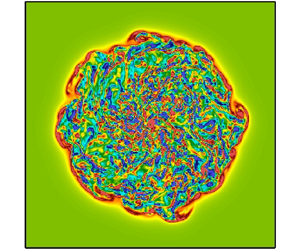
To understand the flow features near the bottom boundary, we plotted the contours of vertical vorticity  $(\unicode[STIX]{x1D714}_{3})$ in a horizontal $(x_{1}{-}x_{2})$ plane near the bottom boundary $(x_{3}/L_{3}=-0.95)$, as shown in figure 9. The plots are shown at $t\approx 251~\text{s}$ for all cases. This time instants correspond to 5.4, 2.9, 1.16 inertial periods for $Ro=0.032$ (DNS8), 0.078 (DNS9) and 0.32 (DNS10), respectively. Figure 9(a,b) shows that the flow in these two cases is already affected by rotation significantly, as evident from the modified structure of the rim current and baroclinic vortices. The rim current is the geostrophic current formed at the interface of a dense and a lighter fluid due to the combination of pressure gradient and Coriolis forces. In this case, the pressure gradient force is directed radially inward and the Coriolis force is directed radially outward, so the rim current is in the azimuthal direction, perpendicular to both the pressure gradient and Coriolis forces. Since the rotation effects are already prominent by this time for $Ro=0.032$, 0.078, the rim current has undergone baroclinic instability, as is evident from the baroclinic vortices in figure 9(a,b). An experimental study by Griffiths & Linden (Reference Griffiths and Linden1981) reported the formation of similar baroclinic vortices when a buoyant fluid is released into a two-layer rotating system. For $Ro=0.32$, $t=251~\text{s}$ corresponds to 1.16 inertial periods, therefore the rim current feels weak rotational effects and is in the process of undergoing baroclinic instability, as shown in figure 9(c). For $Ro=2.2$, the rotation effects are negligible, and therefore there is no evidence of a rim current. The instability of the gravity current spreading along the bottom surface results in small-scale vortices, as shown in figure 9(d).
An interesting feature found from the vorticity field for higher rotation cases is that there is a cyclonic circulation near the top surface, and an anti-cyclonic circulation near the bottom boundary (see movies 1–4 in the supplementary material available at https://doi.org/10.1017/jfm.2020.94). A similar phenomenon is also reported in an observational study near the Greenland Sea (Schott et al. Reference Schott, Visbeck and Fischer1993). In the cases with low rotation rates, cyclonic circulation is observed near the top surface similar to the high rotation cases. However, near the bottom boundary, both cyclonic (inner region) and anti-cyclonic (near the periphery of mixed fluid) circulations are observed.
As mentioned earlier, the effect of rotation is found to be prominent after the first inertial period. Due to the variation of the Coriolis parameter  $f$ among the different cases, the inertial period varies by nearly an order of magnitude (see table 1). For example, at a low rotation rate (DNS13), the inertial period is much longer than in the high rotation cases (DNS8, DNS9). The mixed fluid in DNS13 reaches the bottom boundary and spreads as a gravity current well before the first inertial period. Therefore, comparing the flow evolution at the same dimensional time rather than the same non-dimensional time (based on the inertial period) accentuates the contrasting flow features between the low and high rotation cases.
3.4 Turbulent statistics
As discussed in the previous section, low Rossby number cases reach a quasi-steady state, where further expansion in the lateral directions is inhibited by a balance of Coriolis and pressure gradient forces. However, for the high Rossby number cases, dense fluid plunges down quickly, leading to an increase in turbulence. Therefore, it is important to understand how the turbulence evolves during the convection processes for various Rossby numbers. In this section, a detailed analysis of the root-mean-square (r.m.s.) velocities and turbulent kinetic energy budget is presented.
3.4.1 Root-mean-square velocity
Figure 10 shows the vertical profiles of non-normalized and normalized  $u_{1,rms}$ at intermediate and late times for different rotation rates. The analogous profiles of $u_{3,rms}$ are shown in figure 11. It is evident from figures 10 and 11 that the magnitude of turbulence decreases with increasing rotation rate. In a rotating environment, a fluid parcel experiences a Coriolis force opposing the existing horizontal pressure gradient. At low rotation rates, the horizontal pressure gradient dominates over the Coriolis force, drawing the fluid parcel towards the centre. This fluid parcel eventually plunges and releases its potential energy to turbulent kinetic energy. However, an increase in the rotation rate results in an increased Coriolis force, which is balanced by the horizontal pressure gradient. This horizontal force balance stabilizes the flow by inhibiting the downward motion of the fluid parcel, and hence impedes the release of potential energy to turbulent kinetic energy (Veronis Reference Veronis1970).

Figure 10. Vertical profiles of  $u_{1,rms}$ (a,c) at times $t\approx 151~\text{s}$ and 251 s, respectively. Panels (b,d) show $u_{1,rms}$ normalized by $(B_{0}/f)^{1/2}$. The domain depth is $L_{3}=0.4$ in all cases.

Figure 11. Vertical profiles of  $u_{3,rms}$ (a,c) at times $t\approx 151$ and 251, respectively. Panels (b,d) show $u_{3,rms}$ normalized by $(B_{0}/f)^{1/2}$. The domain depth is $L_{3}=0.4$ in all cases.
The comparison of non-normalized and normalized velocity profiles (figure 10c,d) shows that the normalization with  $(B_{0}/f)^{1/2}$ drifts the profiles apart near the top surface. At the bottom boundary, a jet-like feature is observed at $t=251~\text{s}$. This jet-like feature is attributed to the interaction of the gravity current with the viscous boundary layer. Also, the magnitude of this jet decreases with increasing rotation rate, consistent with the previously discussed idea of the Coriolis force being a stabilizing factor suppressing the conversion of potential energy to kinetic energy. The comparison of non-normalized and normalized $u_{1,rms}$ profiles near the bottom boundary shows that normalization with $(B_{0}/f)^{1/2}$ brings the profiles closer to each other, however, a proper collapse is not achieved. This jet-like feature was absent in the previous numerical study of Jones & Marshall (Reference Jones and Marshall1993) owing to a coarse vertical resolution and high values of the eddy viscosity and thermal diffusivity. The central region also has a trend similar to the bottom boundary. The normalization of the velocity profiles brings them closer to each other, however, the normalized profiles of the lowest rotation rate ( $f=0.008$, DNS13) and the highest rotation rate ( $f=0.134$, DNS8) simulations are still significantly far apart. Some of the previous studies suggested a velocity scaling of $(B_{0}L_{3})^{1/3}$ at lower rotation rates. However, we found that this scaling performs no better than $(B_{0}/f)^{1/2}$ in low rotation cases. In summary, although the velocity field appears to scale with $(B_{0}/f)^{1/2}$ in some regions of the flow, in agreement with previous studies (Jones & Marshall Reference Jones and Marshall1993; Maxworthy & Narimousa Reference Maxworthy and Narimousa1994), there are certain regions (e.g. near the top surface) of the flow where normalization actually results in the velocity profiles drifting apart.
The profiles of  $u_{3,rms}$ at time $t=151~\text{s}$ (figure 11a) show a maximum vertical velocity near the mid-depth location and gradual decrease towards the boundaries. The magnitude of $u_{3,rms}$ also decreases with an increase in rotation rate. At a later time $t=251~\text{s}$, the location of maximum vertical velocity shifts towards the bottom boundary, except for high rotation rates ( $f=0.074$ and 0.134). At low rotation rates, the denser fluid under the effect of gravity collapses onto the bottom boundary. When this denser turbulent fluid hits the bottom solid wall, vertical momentum is transferred into horizontal momentum, as is evident from the jet-like features shown in the $u_{1,rms}$ profiles (figure 10). At high rotation rates, the Coriolis effect prevents the denser fluid from collapsing onto the bottom boundary, and thus prevents conversion of vertical momentum into horizontal momentum. An interesting phenomenon occurs at an intermediate rotation rate of $f=0.029~\text{s}^{-1}$, corresponding to a $Ro=0.32$, where the upper half of the profile resembles higher rotation rates and the bottom half of the profile resembles lower rotation rates.
3.4.2 Turbulent kinetic energy budget
An analysis of the turbulent kinetic energy (TKE) budget is presented in this section to understand the role of turbulent energetics in the deep-ocean convection process. We compute the various terms of the TKE budget equation as follows:
 $$\begin{eqnarray}\frac{\text{d}(TKE)}{\text{d}t}=P+B-\unicode[STIX]{x1D700}-\frac{\unicode[STIX]{x2202}\mathfrak{T}_{\mathfrak{i}}}{\unicode[STIX]{x2202}x_{i}}-\unicode[STIX]{x1D700}_{sgs}-\frac{\unicode[STIX]{x2202}\mathfrak{T}_{\mathfrak{i},\mathfrak{s}\mathfrak{g}\mathfrak{s}}}{\unicode[STIX]{x2202}x_{i}},\end{eqnarray}$$
where
 $$\begin{eqnarray}P=-\langle u_{i}^{\prime }u_{j}^{\prime }\rangle \frac{\text{d}U_{i}}{\text{d}x_{j}},\quad B=-\frac{g}{\unicode[STIX]{x1D70C}_{0}}\langle \unicode[STIX]{x1D70C}^{\prime }u_{3}^{\prime }\rangle ,\end{eqnarray}$$
are the turbulent production and turbulent buoyancy flux respectively,
 $$\begin{eqnarray}\unicode[STIX]{x1D700}=2\unicode[STIX]{x1D708}\langle s_{ij}^{\prime }s_{ij}^{\prime }\rangle ,\end{eqnarray}$$
 is the turbulent dissipation rate, where  $s_{ij}^{\prime }=\frac{1}{2}((\unicode[STIX]{x2202}u_{i}^{\prime }/\unicode[STIX]{x2202}x_{j})+(\unicode[STIX]{x2202}u_{j}^{\prime }/\unicode[STIX]{x2202}x_{i}))$ is the turbulent strain rate and $\unicode[STIX]{x2202}\mathfrak{T}_{\mathfrak{i}}/\unicode[STIX]{x2202}x_{i}$ is the transport term where
 $$\begin{eqnarray}\mathfrak{T}_{\mathfrak{i}}=\frac{1}{2}\langle u_{i}^{\prime }u_{j}^{\prime }u_{j}^{\prime }\rangle +\frac{\langle u_{i}^{\prime }p^{\prime }\rangle }{\unicode[STIX]{x1D70C}_{0}}-2\unicode[STIX]{x1D708}\langle u_{j}^{\prime }s_{ij}^{\prime }\rangle .\end{eqnarray}$$
 The subgrid dissipation  $\unicode[STIX]{x1D700}_{sgs}$ is defined as:
 $$\begin{eqnarray}\unicode[STIX]{x1D700}_{sgs}=-\left\langle \unicode[STIX]{x1D70F}_{ij}^{\prime }\frac{\unicode[STIX]{x2202}\overline{u_{i}^{\prime }}}{\unicode[STIX]{x2202}x_{j}}\right\rangle .\end{eqnarray}$$
 The subgrid transport  $\unicode[STIX]{x2202}\mathfrak{T}_{\mathfrak{i},\mathfrak{s}\mathfrak{g}\mathfrak{s}}/\unicode[STIX]{x2202}x_{i}$ is calculated as:
 $$\begin{eqnarray}\frac{\unicode[STIX]{x2202}\mathfrak{T}_{\mathfrak{i},\mathfrak{s}\mathfrak{g}\mathfrak{s}}}{\unicode[STIX]{x2202}x_{i}}=\langle \unicode[STIX]{x1D70F}_{ij}^{\prime }\overline{u_{i}^{\prime }}\rangle .\end{eqnarray}$$
The subgrid dissipation and transport terms are zero for DNS.

Figure 12. TKE budget,  $Ro=0.32$ (DNS10 in table 1): (a) all the terms in the TKE budget at time $t=251~\text{s}$, (b) time evolution of vertically integrated TKE budget terms. TKE budget, $Ro=0.32$ (LES6 in table 2): (c) all the terms in the TKE budget at time $t=20.5~\text{h}$, (d) time evolution of vertically integrated TKE budget terms. TKE budget, $Ro=0.32$ (LES7 in table 3): (e) all the terms in the TKE budget at time $t=20.5~\text{h}$, (f) time evolution of vertically integrated TKE budget terms.
Figures 12(a), 12(c) and 12(e) show all the terms of the TKE budget equation for DNS10, LES6 and LES7 for  $Ro=0.32$ at $t\approx 251~\text{s}$ and 20.5 h, respectively. The shear production term $P$ is negligible at all times for both DNS and LES owing to the absence of externally imposed shear. The transport term for both DNS and LES has some spatial variability owing to the turbulence, however, the vertically integrated values are negligible compared to the dominant terms in the budget. The turbulent buoyancy flux $B$ for both DNS and LES is the primary source of turbulence whereas the turbulent dissipation rate is the energy sink. Figures 12(a), 12(c) and 12(e) show that energy transfer to turbulence occurs near the top surface, as evident from the high turbulent buoyancy flux between $x_{3}/L_{3}=0$ and $x_{3}/L_{3}\approx -0.5$. The dissipation rate ( $\unicode[STIX]{x1D700}$ for DNS10, $\unicode[STIX]{x1D700}$ and $\unicode[STIX]{x1D700}_{sgs}$ for LES6, $\unicode[STIX]{x1D700}_{sgs}$ for LES7) is maximum near the bottom boundary, suggesting that the interaction of the mixed fluid with the viscous boundary layer plays an important role in the energy dissipation.
Figures 12(b), 12(d) and 12(f) show the time evolution of the vertically integrated TKE budget terms. All quantities are negligible until  $t\approx 50~\text{s}$ for DNS and $t\approx 3~\text{h}$ for LES as the flow remains laminar. At a later time, due to the conversion from potential energy to TKE by means of turbulent buoyancy flux $B$, the flow turns turbulent and small-scale features appear. The ‘Balance’ term (represented by the green dashed curve) in figures 12(b), 12(d) and 12(e) is the sum of all the quantities on the right-hand side of the TKE budget equation (3.4). Close agreement between the ‘Balance’ term and the unsteady term $\text{d}(TKE)/\text{d}t$ shows that the residual is small and the TKE budget closure is well maintained for both DNS and LES. A nominal value of residual ( $\text{d}(TKE)/\text{d}t$ – Balance) also suggests that the grid spacing considered in DNS is small enough to resolve the smallest scales of turbulence. It also signifies that the large scales are well resolved in LES, and the Smagorinsky model is able to parameterize the small scales accurately. It is important to note that the increase in dissipation rate for DNS (figure 12b) is small until $t\approx 100~\text{s}$, but a sudden jump is observed when $t>100~\text{s}$. This is due to the fact that the dense turbulent fluid reaches the bottom boundary at $t\approx 100~\text{s}$ and the subsequent interaction of the turbulent fluid with the bottom boundary increases the dissipation rate substantially. Similarly, in LES6, a uniform increase in both resolved and subgrid dissipation is observed after $t\approx 5.5~\text{h}$, signifying the interaction of the dense fluid with the bottom boundary. For DNS, at $t>210~\text{s}$, the turbulent quantities reach a quasi-steady state, with the unsteady term close to zero, and the turbulent buoyancy flux is approximately balanced by the turbulent dissipation rate. A similar quasi-steady state is observed in LES cases for $t>20.5~\text{h}$. We have also analysed the flow evolution at a later time (not shown in the figure) and found that the buoyancy flux and $\text{d}(TKE)/\text{d}t$ terms oscillate around the steady state values, whereas the dissipation term remains similar. Closure of the TKE budget is also achieved for the rest of the cases in tables 1 and 2.
In DNS, since all the scales of the flow are explicitly resolved, dissipation is entirely contributed by the resolved scales of the flow. However, in LES, dissipation has contributions from both the resolved and subgrid scales of the flow. The ratio between the largest and the smallest scales of the flow increases with increasing  $Ra$. Even though the grid resolution is exactly the same for LES6 and LES7, owing to the difference in $Ra$, the fraction of the scales explicitly resolved in LES7 is much smaller than in LES6. Owing to this, the resolved dissipation is much smaller as compared to the subgrid-scale dissipation in LES7.
4 Conclusions
Three-dimensional direct numerical simulations and large eddy simulations are performed to investigate the dynamics of deep-ocean convection in a stratified rotating framework. DNS are performed at laboratory scales and LES are carried out at large scales ( $O$(10 km)) to understand the effect of the imposed surface buoyancy flux and background rotation rate on the dynamics of deep-ocean convection. The Rossby numbers in both DNS and LES are kept relevant to the real ocean convection, varying from 0.032 (high rotation rates) to 2.2 (low rotation rates). The highest Rayleigh number that is considered in the present simulations is $10^{26}$, which lies within the range of Rayleigh numbers, $10^{25}{-}10^{31}$, typically observed in the ocean (Maxworthy & Narimousa Reference Maxworthy and Narimousa1994). Each DNS uses approximately half a billion grid points with a grid spacing fine enough to resolve the small-scale turbulence. As evident from the horizontal spectra of turbulent kinetic energy, the Kolmogorov length scale is well resolved in DNS. Similarly, turbulent eddies are well resolved in LES, as evident from the energy spectrum showing an approximately four orders of magnitude drop in the energy.
The initial evolution of the flow ( $t\ll 2\unicode[STIX]{x03C0}/f$) manifests downward moving dense fluid columns (plumes) with a well-defined shape. We proposed a scaling for the diameter and velocity of these plumes based on the balance between the leading-order terms in the vertical velocity and temperature equations. Surface flux magnitude $B_{0}$ and thermal (eddy) diffusivity $\unicode[STIX]{x1D705}_{t}(\unicode[STIX]{x1D705}_{sgs})$ were used to quantify the initial plume characteristics. The Coriolis parameter was not considered to characterize initial flow evolution as the rotation effects are found to be negligible when $t<2\unicode[STIX]{x03C0}/f$. We found a reasonably good agreement between the theoretical values of the plume diameter and velocity when compared with the corresponding values obtained from the numerical simulations. We also found that varying the rotation rate at a particular surface flux magnitude does not change the early plume characteristics. It is important to note that the scaling proposed here for initial flow evolution may have limited applicability when the flow is dominated by background rotation or in the presence of background shear, both of which can alter the plume characteristics significantly. It is possible that, in situations where the surface cooling is observed to be localized and the rotation effects are not prominent, the plume characteristics at real ocean convection sites can be deduced from the scalings proposed in this study. However, this conjecture warrants further investigation at various test sites where deep-ocean convection is observed.
At time  $t>2\unicode[STIX]{x03C0}/f$, the rotational effects become important and the flow evolution can be understood by considering a balance between the Coriolis and pressure gradient forces. At low rotation rates ( $Ro>0.32$), denser fluid formed due to surface cooling plunges quickly, hits the bottom boundary and spreads as a gravity current. At high rotation rates $Ro<0.32$, the denser fluid spreads in the lateral directions before reaching the bottom boundary and attains a quasi-steady state with an approximate balance between the pressure gradient and Coriolis forces. An interesting feature observed at higher rotation rates is the formation of the rim current at the periphery of the mixed fluid. The lateral density gradient that exists at the interface comes under the influence of rotation and forms the rim current, similar to the geostrophic current observed in the oceans. This rim current undergoes baroclinic instability, resulting in the formation of baroclinic vortices and turbulent eddies which augment the mixing rate.
The r.m.s. velocities are found to decrease with an increase in rotation rate, in agreement with the previous studies by Raasch & Etling (Reference Raasch and Etling1998) and Jones & Marshall (Reference Jones and Marshall1993). High rotation acts as a stabilizing agent by establishing a balance between the horizontal pressure gradient and the Coriolis force. This horizontal force balance inhibits the plummeting of the fluid parcels and hence hinders the conversion of potential energy to turbulent kinetic energy. The r.m.s. velocity profiles manifest a jet-like feature (figure 11) near the bottom boundary for  $Ro\geqslant 0.32$. This qualitative feature of the flow can only be observed when the grid resolution in the vertical direction is fine enough to capture the boundary layer dynamics. The vertical grid resolution of Jones & Marshall (Reference Jones and Marshall1993) was not fine enough to capture this feature.
In summary, the initial flow evolution is found to be governed by a balance between the diffusion and buoyancy flux while the rotation effects are negligible. At a later time, the rotational effects become important and the scaling proposed by Jones & Marshall (Reference Jones and Marshall1993) can predict flow quantities to a good extent. However, it is important to note that, in certain regions of the flow, for example, near the top surface where the rotational effects on plumes are negligible, normalization of the  $u_{1,rms}$ velocity profiles with the scaling proposed by Jones & Marshall (Reference Jones and Marshall1993) results in a drifting apart of the profiles rather than a collapse of the profiles. Overall, this study gave us insights into the relative importance of buoyancy flux, diffusion and rotation rate at various stages of the flow evolution. The role of background stratification in the flow evolution will be considered in a future study, especially when the ambient is strongly stratified ( $N/f>1$).
Acknowledgements
This research used resources of the Oak Ridge Leadership Computing Facility, which is a DOE Office of Science User Facility supported under Contract DE-AC05-00OR22725. The code used in this study is available athttps://github.com/itsanikesh/OCONVECTION.git. This repository also contains the set-up files for all the DNS and LES cases.
Declaration of interests
The authors report no conflict of interest.
Supplementary movies
Supplementary movies are available at https://doi.org/10.1017/jfm.2020.94.
Appendix A
Since the Coriolis effects become prominent at a later time (i.e. at  $t>2\unicode[STIX]{x03C0}/f$), there must be another time scale which governs the initial evolution of the plumes. The scaling for initial flow evolution can be obtained by considering leading-order terms in the vertical momentum ( $i=3$ in (2.2)) and temperature deviation (2.3) equations. First, considering the temperature deviation equation, the leading-order balance will be between the advection and the diffusion terms as shown below:
 $$\begin{eqnarray}\displaystyle & \displaystyle U_{3,i}\frac{\text{d}\widetilde{T}}{\text{d}x_{3}}\sim \unicode[STIX]{x1D705}_{t}\frac{\text{d}^{2}\widetilde{T}}{\text{d}x_{3}^{2}}, & \displaystyle\end{eqnarray}$$
 $$\begin{eqnarray}\displaystyle & \displaystyle U_{3,i}\frac{\widetilde{T}}{h}\sim \unicode[STIX]{x1D705}_{t}\frac{\widetilde{T}}{h^{2}}, & \displaystyle\end{eqnarray}$$
 $$\begin{eqnarray}\displaystyle & \displaystyle U_{3,i}h\sim \unicode[STIX]{x1D705}_{t}, & \displaystyle\end{eqnarray}$$
 where  $h$ is the vertical length scale, $U_{3,i}$ is the vertical velocity scale associated with plumes.
Now, considering the vertical momentum equation, the balance will be between the advection and the buoyancy terms as shown below:
 $$\begin{eqnarray}U_{3,i}\frac{\text{d}U_{3,i}}{\text{d}x_{3}}\sim \frac{g\tilde{\unicode[STIX]{x1D70C}}}{\unicode[STIX]{x1D70C}_{0}}.\end{eqnarray}$$
 Multiplying the above equation with  $U_{3,i}$, we obtain
 $$\begin{eqnarray}\displaystyle & \displaystyle U_{3,i}^{2}\frac{\text{d}U_{3,i}}{\text{d}x_{3}}\sim \frac{g\tilde{\unicode[STIX]{x1D70C}}U_{3,i}}{\unicode[STIX]{x1D70C}_{0}}, & \displaystyle\end{eqnarray}$$
 $$\begin{eqnarray}\displaystyle & \displaystyle U_{3,i}^{2}\frac{U_{3,i}}{h}\sim B_{0}, & \displaystyle\end{eqnarray}$$
 $$\begin{eqnarray}\displaystyle & \displaystyle \frac{U_{3,i}^{3}}{h}\sim B_{0}. & \displaystyle\end{eqnarray}$$
 Now, we obtain the scaling for  $U_{3,i}$ by eliminating $h$ from (3.3) and (3.7), as given below:
 $$\begin{eqnarray}U_{3,i}\sim (\unicode[STIX]{x1D705}_{t}B_{0})^{1/4}.\end{eqnarray}$$
Based on the dimensional analysis, the time scale can be obtained as
 $$\begin{eqnarray}{\mathcal{T}}_{i}\sim \left(\frac{\unicode[STIX]{x1D705}_{t}}{B_{0}}\right)^{1/2}.\end{eqnarray}$$
 Now, from the continuity equation, we know that  $U_{1,i}/D_{i}\sim U_{3,i}/h$, where $D_{i}$ is the horizontal length scale associated with the plumes. However, the horizontal and vertical velocity scales, $U_{1,i}$ and $U_{3,i}$, have similar magnitudes during the initial flow evolution. Thus, the horizontal length scale associated with the plume $D_{i}$ can be obtained as
 $$\begin{eqnarray}D_{i}\sim U_{3,i}\times {\mathcal{T}}_{i}\sim \left(\frac{\unicode[STIX]{x1D705}_{t}^{3}}{B_{0}}\right)^{1/4}.\end{eqnarray}$$


