


1. Introduction
Remarkable variations in mixing rates have been observed at river confluences. For instance, Cook & Richmond (Reference Cook and Richmond2004) discussed images of both slow and fast mixing at the same confluence on different dates, with complete mixing occurring after a short distance into the postconfluent reach on one date and a much longer distance on another. Lane et al. (Reference Lane, Parsons, Best, Orfeo, Kostaschuk and Hardy2008) also noted impressive variations in mixing at a very large confluence in South America in two consecutive years. While Cook & Richmond (Reference Cook and Richmond2004) attributed the fast mixing rate to a thermal density difference, Lane et al. (Reference Lane, Parsons, Best, Orfeo, Kostaschuk and Hardy2008) cited bed discordance and inertial effects, yet noted (on p. 14): ‘The possible contribution of density differences [due to suspended sediment gradients] to near-field mixing remains an issue that needs further research’. At a smaller confluence, Rhoads & Sukhodolov (Reference Rhoads and Sukhodolov2001) measured flow from a cooler tributary downwelling under a warmer tributary, forming a helical pattern in temperature contours, a pattern also repeated in the velocity field. Rhoads & Sukhodolov (Reference Rhoads and Sukhodolov2001) emphasised planform flow curvature, yet later work at the site stressed the importance of thermal density differences influencing these patterns (Lewis & Rhoads Reference Lewis and Rhoads2015). Whether caused by gradients in temperature, suspended sediments or dissolved minerals, it is becoming increasingly clear that small density differences (< 0.75 kg m $^{-3}$) dramatically affect a confluence's mixing processes (Cook & Richmond Reference Cook and Richmond2004; Lyubimova et al. Reference Lyubimova, Lepikhin, Konovalov, Parshakova and Tiunov2014; Ramón et al. Reference Ramón, Armengol, Dolz, Prats and Rueda2014; Duguay, Biron & Lacey Reference Duguay, Biron and Lacey2022a; Jiang et al. Reference Jiang, Constantinescu, Yuan and Tang2022; Li et al. Reference Li, Tang, Yuan, Xiao, Xu, Huang, Rennie and Gualtieri2022), though the extents to which, and the mechanisms by which remain unclear.
Examples of gravity currents in nature occur where cool rivers enter warm lakes (Kostaschuk et al. Reference Kostaschuk, Nasr-Azadani, Meiburg, Wei, Chen, Negretti, Best, Peakall and Parsons2018), concentrated saline channels flow on the ocean's floor (Thomas Reference Thomas2001; Parsons et al. Reference Parsons, Peakall, Aksu, Flood, Hiscott, Beşiktepe and Mouland2010) and where tidal circulation causes brackish water to stratify in estuaries and straits (Hansen & Rattray Reference Hansen and Rattray1965). The classic lock exchange, in which two adjacent vertical volumes of fluid of different density are released to stratify vertically and mix, is the most basic form of gravity current (Rottman & Simpson Reference Rottman and Simpson1983). Lock exchanges are vertical shear flows characterised by corotating streamwise-orientated Kelvin–Helmholtz (KH) instabilities along the mixing interface of the two fluids (Brown & Roshko Reference Brown and Roshko1974; Winant & Browand Reference Winant and Browand1974). Gravity currents at river confluences are different. First, the converging rivers develop a horizontal shear flow confined between the bed and the free surface. Second, the vertically oriented KH instabilities typical of horizontal shear flows can be strongly altered as the mixing interface slumps due to the density-induced hydrostatic pressure gradient across the mixing interface (White & Helfrich Reference White and Helfrich2013). Third, the dense front is forced laterally under the lighter tributary, which is converging towards the mixing interface, as opposed to an initially quiescent body of fluid such as in a lock exchange. Therefore, confluences with a density difference ( $\Delta \rho$) are most appropriately categorised as shallow, gravitationally adjusted horizontal shear flows, similar to those investigated by White & Helfrich (Reference White and Helfrich2013). They are expected to share characteristics of both free shear flows (i.e. vertical KH vortices produced by horizontal shear) and gravity currents (i.e. streamwise KH instabilities on the slumping mixing interface Rottman & Simpson Reference Rottman and Simpson1983; Cantero et al. Reference Cantero, Lee, Balachandar and Garcia2007), yet are more complex due to the interactions of these flow processes with other complications caused by the confluence's planform geometry, momentum ratio, bathymetry and bed roughness (Chu & Babarutsi Reference Chu and Babarutsi1988).
Little is known of the gravity currents common to confluences. Most work has focused on assessing time-averaged vertical stratification caused by the slumping mixing interface. Cook & Richmond (Reference Cook and Richmond2004) showed this, as did Biron & Lane (Reference Biron and Lane2008) and numerous other numerical and field studies since (Lyubimova et al. Reference Lyubimova, Lepikhin, Konovalov, Parshakova and Tiunov2014; Ramón et al. Reference Ramón, Armengol, Dolz, Prats and Rueda2014; Ramón, Prats & Rueda Reference Ramón, Prats and Rueda2016; Cheng & Constantinescu Reference Cheng and Constantinescu2018; Horna-Munoz et al. Reference Horna-Munoz, Constantinescu, Rhoads, Lewis and Sukhodolov2020; Pouchoulin et al. Reference Pouchoulin, Le Coz, Mignot, Gond and Riviere2020; van Rooijen et al. Reference van Rooijen, Mosselman, Sloff and Uijttewaal2020; Cheng & Constantinescu Reference Cheng and Constantinescu2022). What is less known, is how the inertial attributes of the confluence alter the gravity current's secondary flow structure and dynamics. Some progress has been made with numerical models. Notably, van Rooijen et al. (Reference van Rooijen, Mosselman, Sloff and Uijttewaal2020) showed that strong slumping can hamper, or even eliminate vertically orientated coherent structures entirely. Horna-Munoz et al. (Reference Horna-Munoz, Constantinescu, Rhoads, Lewis and Sukhodolov2020) identified streamwise-orientated KH instabilities on the slumped mixing interface (i.e. interfacial instabilities) and detected streamwise-oriented vortices (SOVs) in the time-averaged flow field, yet attributed them to causes other than density differences (i.e. downwelling superelevated flow). Cheng & Constantinescu (Reference Cheng and Constantinescu2022) also detected numerous corotating, density-induced SOVs on the slumped mixing interface of a parallel channel resembling the horizontal KH instabilities mentioned by Horna-Munoz et al. (Reference Horna-Munoz, Constantinescu, Rhoads, Lewis and Sukhodolov2020).
Recently, Duguay et al. (Reference Duguay, Biron and Lacey2022a) suggested that SOVs observed at the Coaticook- Massawippi confluence (Quebec, Canada) were a confined gravity current, based on eddy-resolved numerical modelling considering buoyant forces. This spiralling gravity current is formed when the dense front and its lighter counterpart that is pulled laterally above due to the incompressibility constraint, extend laterally downstream from the confluence's apex and become confined between the flows of the converging tributaries. More specifically, as the fronts encounter sufficient momentum from the opposing channel, the dense front is deflected above itself and the light front downwards, resulting in a strongly coherent density-driven SOV (see supplementary movie 1 of Duguay et al. Reference Duguay, Biron and Lacey2022a). In a follow-up study, Duguay, Biron & Lacey (Reference Duguay, Biron and Lacey2022b) showed that under identical hydraulic conditions, reversing the direction of  $\Delta \rho$ caused either highly coherent density SOVs or less coherent streamwise KH instabilities to form, with the difference attributed to whether the dense front protruded into the slow or fast tributary, respectively. Consequently, the dynamics of the secondary flow are altered by the inertial attributes of the channels and their difference in density, a subject of which we know little, and of which recent attempts to describe mixing dynamics at river confluences make no account (e.g. Sukhodolov et al. Reference Sukhodolov, Shumilova, Constantinescu, Lewis and Rhoads2023).
To the authors’ knowledge, the effects of  $\Delta \rho$ on confluence hydrodynamics, the proposed confined gravity current and the coherent flow structures it produces have not yet been studied in a controlled laboratory setting. Our objective is therefore to empirically investigate how gravity currents behave at river confluences, with the aim of identifying the hydrodynamic and densimetric conditions necessary to produce strongly coherent density SOVs similar to those observed at the Coaticook-Massawippi confluence. To this end, experiments are carried out in a laboratory confluence allowing a spectrum of thermally induced density differences of similar magnitude to that common to many natural mesoscale confluences. Spatially and temporally resolved flow field measurement and visualisation techniques provide insights into the dynamic density-driven secondary flow structure of the confluence's mixing interface.
2. Methods
2.1. Flume and water supply
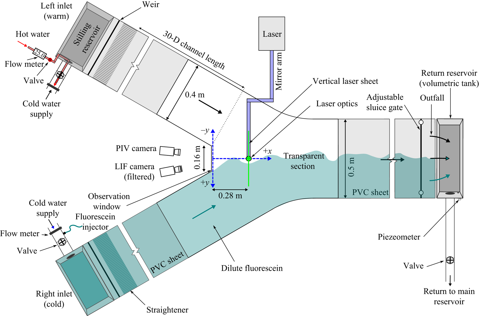
Experiments were conducted in a flatbed (zero slope), open-channel, symmetric laboratory confluence with a 60  $^{\circ }$C junction angle at the Université de Sherbrooke's Hydraulics laboratory (figure 1). The central section has a clear, transparent polycarbonate bed and walls to allow optical access to the mixing interface for particle image velocimetry (PIV) and laser-induced fluorescence (LIF) experiments. The flume walls are 0.11 m high, with upstream tributary channels 2.6 m long and downstream channels 1.5 m long. A 0.16 m wide clear polycarbonate observation window was fitted for the vertical wall at the apex. Cold water was supplied to the flume from a constant head tank on the facility's roof, to which water was pumped from a large subterranean reservoir ( $\approx$100 m $^{3}$). Flow from the tank passed through a sand filter to remove large particulate matter before entering the flume. The discharges in each channel were adjusted separately by valves with flow measurements obtained from ultrasonic flow meters on the inflow pipes. Discharges entered upstream of each channel first by passing into a stilling basin, then under a sluice gate, before flowing through a series of perforated stainless steel flow straighteners. The water depth in the flume where the PIV and LIF measurements were performed was kept constant through all experiments at $D = 0.07$ m (at 0.28 m from the apex at the PIV imaging plane, see figure 1) and was set by adjusting a sluice gate at the downstream end of the flume. Lateral variations in the water surface elevation were imperceptible in measured traverses with a point gauge. The flow exiting the sluice gate fell into a rectangular reservoir fitted with a piezometer and a valve on its exit pipe to enable volumetric discharge measurements to calibrate the ultrasonic flow meters.
Details of the experimental flume used to study the secondary flow structure in the mixing interface of a 60 $^{\circ }$ symmetric confluence with a temperature-induced $\Delta \rho$ between both channels.
2.2. Thermal density difference
The flume was designed so the left channel's density could be lowered by increasing its temperature relative to that of the right channel. This was done to permit experiments with a density difference ( $\Delta \rho$) between the two channels. Density differences were achieved by mixing hot water of discharge $Q_{h}$ and temperature $T_{h}$ ( $_h$ for hot) supplied from the building (more details below) with cold water of discharge $Q_{c}$ and temperature $T_{c}$ ( $_c$ for cold) from the laboratory's mainline head tank, producing a mixed warm flow of temperature ( $T_{l}$) and discharge $Q_{l}$ in the left channel ( $_l$ for left). The right channel's temperature ( $T_r$, with $_r$ indicating right) was the same as the cold water from the head tank (i.e. $T_{c}$). The discharges $Q_{c}$ and $Q_{h}$ required to produce the nominal thermally induced $\Delta \rho$ were calculated in four steps. First, the density of the left channel,
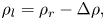 \begin{equation} \rho_{l} = \rho_{r} - \Delta\rho, \end{equation}
was determined knowing the target value of  $\Delta \rho$ and the density of the colder right channel ( $\rho _{r}$) calculated using
 \begin{align} \rho &= 999.84847 + 6.337563 \times 10^{{-}2}T \nonumber\\ &\quad - 8.523829 \times 10^{{-}3}T^{2} + 6.943248 \times 10^{{-}5}T^{3} \nonumber\\ &\quad - 3.821216 \times 10^{{-}7}T^{4}, \end{align}
where  $\rho$ is the density of air-saturated water at temperature ( $T$) (Jones & Harris Reference Jones and Harris1992). Second, (2.2) was reapplied and iterated to solve for $T_{l}$ necessary to produce $\rho _{l}$. Third, by performing various substitutions and rearrangements of the thermal energy conservation equation,
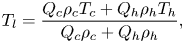 \begin{equation} T_{l}=\frac{Q_{c}\rho_{c}T_{c}+Q_{h}\rho_{h}T_{h}}{Q_{c}\rho_{c}+Q_{h}\rho_{h}}, \end{equation}
it can be shown to result in
 \begin{equation} 0=\frac{Q_{h}}{Q_{l}- Q_{h}}-\frac{\rho_{c}(T_{l}-T_{c})}{(\rho_{c}-\Delta\rho)(T_{h}-T_{l})} \end{equation}
which was iterated for  $Q_{h}$. Finally, $Q_{c}$ was obtained with,
 \begin{equation} Q_{c}=Q_{l}-Q_{h}. \end{equation}
 Hot water was supplied from the building to a 200 litre (L) reservoir with a small constant head tank (20 L) inside of it. Hot water from the 200 L reservoir was pumped into the small tank connected to the left channel's cold water supply by a pipe. Here  $Q_h$ was regulated by a valve to readings from an electromagnetic flow meter (Picomag DN20) installed on the pipe. The constant head tank ensured a stable $Q_{h}$ during the experiments. The temperature $T_h$ supplied from the building could vary between $\approx$45 $^{\circ }$C and 52 $^{\circ }$C for reasons beyond our control and $T_c$ could also vary between 15 $^{\circ }$C and 19 $^{\circ }$C as it warmed in the piping network during a given experimental day ( $\approx$0.5 $^{\circ }$C h $^{-1}$). Due to these drifts, values of $T_h$ and $T_c$ were measured immediately before each experiment and used to update $Q_h$ and $Q_c$ to produce the targeted $\Delta \rho$. Flow measurements required less than 5 min and no temperature differences measured before and after a given experiment were detected. For each experiment, measured $T_l$ were within $\pm$0.2 $^{\circ }$C the nominal value necessary to produce $\rho _l$ calculated using (2.2).
2.3. Tested flow conditions
The depth, velocity and density conditions were chosen based on the following considerations: (1) to respect similitude with many natural mesoscale confluence Froude numbers and  $\Delta \rho$ magnitudes, such as those of the Coaticook-Massawippi confluence; and (2) constraints related to limited laboratory space, laser safety protocol, refraction issues related to the mixing of water of different densities (problematic for PIV at higher values of $\Delta \rho$), available hot water discharge and considerations related to performing out-of-plane PIV (e.g. out-of-plane velocities cannot be too fast).
Table 1 summarises the three sets of density conditions studied: equal density ( $\Delta \rho = 0.00$ kg m $^{-3}$, labelled $eq$), low ( $\Delta \rho = 0.33$ kg m $^{-3}$) and high ( $\Delta \rho = 0.66$ kg m $^{-3}$) labelled $lo$ and $hi$, respectively. The bulk velocity of the right channel ( $U_r$) was held constant at 0.071 m s $^{-1}$, and two different bulk velocities were tested in the left channel ( $U_l$): fast (0.071 m s $^{-1}$, subscript 1) and slow (0.039 m s $^{-1}$, subscript 2). Depth ( $D$) was 0.07 m in all experiments. These variations were chosen to study how the difference in momentum between the dense and light channel modifies the density-driven secondary flow structure, with the $eq$ experiments providing a baseline in the absence of $\Delta \rho$. The ratio of the dense channel's momentum (always the right channel) to the light (left) channel's momentum is expressed as
 \begin{equation} Mr_{D} = \frac{\rho_{r}Q_{r}U_{r}}{\rho_{l}Q_{l}U_{l}}, \end{equation}
and provides a means to overcome the ambiguity associated with choosing a main channel in the symmetric confluence, but also as a means to parameterise the potential of the dense channel to deflect the flow of the light channel. The  $Mr_{D}$ of the cases are presented in table 1.
Flow properties. Here  $\Delta \rho$ is the density difference; $Q_{l}$, $Q_{r}$ the flow rates of the right and left channels, respectively; $Q_{l}/Q_{r}$ the discharge ratio; $Mr_{D} = \rho _{r}Q_{r}U_{r}/\rho _{l}Q_{l}U_{l}$ the density momentum ratio; $\boldsymbol {F}_{l}$, $\boldsymbol {F}_{r}$ the Froude number of the left and right channels; $\boldsymbol {Re}_{l}$, $\boldsymbol {Re}_{r}$ the Reynolds number of the left and right channels.
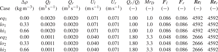
The Froude number of the left channel ( $\boldsymbol {F}_r = U/\sqrt {gD}$, where $U_l$ is taken as $U$) in the slow experiments was 0.048, similar in magnitude to the $\boldsymbol {F}_{r}$ of 0.04 of the Massawippi during the density SOV observations of Duguay et al. (Reference Duguay, Biron and Lacey2022b). The Froude number of the right channel ( $\boldsymbol {F}_r = 0.086$) is also of similar magnitude to that of the Coaticook (0.12) in Duguay et al. (Reference Duguay, Biron and Lacey2022b). The values of $\Delta \rho$ straddle that of 0.50 kg m $^{-3}$ estimated between the Coaticook and Massawippi rivers during the coherent density SOV observations of July 9th, 2020, discussed by Duguay et al. (Reference Duguay, Biron and Lacey2022a). Scaling is not done with the densimetric Froude number for reasons discussed in § 4.3.
2.4. Particle image velocimetry and laser-induced fluorescence
Particle image velocimetry was used to quantify the flow field. During the experiments, LIF was also performed simultaneously with PIV to visualise the corresponding flow structure. A Q-switched, dual-cavity Nd:YLF laser with a wavelength of 532 nm and maximum energy of 20 mJ at 200 Hz was used as the light source for the PIV and LIF experiments. The laser beam was directed through a mirror arm and optics (see figure 1) to form a  $\approx$2 mm thick by 0.20 m wide light sheet used to illuminate PIV seeding and perform LIF experiments. The cold water supply was seeded with near neutrally buoyant, fused borosilicate glass hollow microspheres ( $\text {median diameter} = 10\,\mathrm {\mu }$m, Sphericel, 110P8). A high-speed controller synchronized two Phantom Miro M110 high-speed video cameras fitted with a 50 mm Nikkon lens (AF NIKKOR 50 mm f/1.4D) to the laser pulses. The fluid imaging software DaVis (version 8.3.1) was used to control the PIV and LIF imaging equipment.
The light sheet was positioned at 4 $D$ from the apex parallel to the transparent observation window (figure 1). A left and right camera looked through the observation window. The left camera recorded the movements of seeding particles to estimate the lateral ( $v$) and vertical ( $w$) velocity components (2C) on the two-dimensional (2D) $yz$ plane using 2C2D-PIV. The right camera captured the LIF images. To produce LIF visualisations, a rotometer (Aalborg, Orangeburg, New York, part P11A1-BB0A-034-39-ST) controlled the flow rate of a concentrated solution of fluorescein into the right channel. When exposed to 532 nm light, the dye mixed in $Q_{r}$ emitted longer wavelength light. To capture clear images of this light, the right camera was fitted with a 540 nm long-pass filter, thus blocking all 532 nm laser light. This 2C2D-PIV and LIF set-up allowed simultaneous time-resolved measurements and visualizations of secondary flow patterns in the mixing interface over a cross-section at 4 $D$.
$D$.
To further illustrate the dynamics of the mixing interface, a single camera LIF experiment was performed on the  $hi_2$ case with the laser sheet positioned at $\tilde {z} = 0.5$ parallel to the bed and centred laterally at $\tilde {x} = 4$ (i.e. 4 $D$). The laser sheet was shone through the apex's observation window, with the LIF camera looking upwards through the polycarbonate bottom. This single camera LIF configuration allowed a qualitative analysis of the dynamics of the lateral flow structures in the mixing interface.
All experiments were performed at a pulse frequency of 200 Hz ( $\Delta t = 0.005$ s), the laser's lowest permissible frequency. Seeding particles on the right side of the field of view, where the fastest out-of-plane components are expected, were visually confirmed to remain illuminated in the light sheet in excess of six frames (0.03 s), indicating the repetition rate of the laser was sufficient to perform out-of-plane PIV. However, cross-correlations between each successive frame produced significant peak locking in the vertical velocity component. Consequently, correlations were instead performed using a three-frame increment (i.e. skipping the set of two intermediary frames). Therefore, of the 8302 images taken in each experiment, 2767 vector fields were measured over a 41.5 s period, for a sampling frequency of 66.7 Hz. Each experimental condition was repeated twice, for a combined measurement period of 83 s. Vectors were calculated using a multipass, shifting and decreasing interrogation window cross-correlation method beginning with $128\times 128$ pixel interrogation windows and ending at 24 pixel $\times$ pixel with a 50 % overlap, for a final spatial resolution of $1.27 \times 10^{-3}$ m. A two-standard-deviation median filter was applied to remove and replace spurious vectors. The final vector field was smoothed with a 3 pixel $^{2}$ Gaussian filter. Flow field statistics were obtained from ensemble averaging the two measurements.
2.5. Non-dimensional variables and symbology
Velocity components measured using PIV, and quantities derived thereof, are presented in non-dimensionalized form using the following scaling conventions. The bulk velocity of the right channel ( $U_{r} = 0.071$ m s $^{-1}$) is used as the velocity scaling parameter. It is always either the faster of the two or equal in velocity to the left channel and it is a constant value for all experiments. The length scaling parameter is the flow depth in the mixing interface (0.07 m) at 4 $D$. The time scale was calculated as $D$/
$D$/ $U_{r}$. Table 2 lists the non-dimensional variables used and their calculation. The time average of a variable ( $\phi$) is denoted by $\bar {\phi }$ and its turbulent fluctuation is denoted as $\phi ^{'}$. Non-dimensionalized variables are indicated by the tilde symbol ( $\tilde {\phi }$).
Dimensionless variables and definitions.

3. Results
3.1. Bulk secondary flow patterns and turbulent statistics
It is useful to begin with an overview of the bulk time-averaged secondary flow patterns measured with 2C2D-PIV (figure 2). As expected, case  $eq_{1}$ is nearly symmetric on both sides of $\tilde {y} = 0$ (figure 2a). Less expectantly, two small, surface-divergent, counter-rotating vortices develop near the surface. In case $eq_{2}$, the lateral symmetry breaks due to the excess momentum of the right channel. A distinct anticlockwise rotating vortex forms near the surface to the left of $\tilde {y} = 0$ (figure 2b). When a small $\Delta \rho$ of 0.33 kg m $^{-3}$ is introduced in $lo_{1}$, the mixing interface (band of $\overline {\tilde {U}}_{v,w}< 0.09$) tilts at an angle of $\approx$33.7 $^{\circ }$ from the bed and a clockwise rotating secondary flow cell forms with its core located at $\tilde {z}\approx 0.75$ (figure 2c). Now, decreasing the velocity in the left channel in case $lo_{2}$, the lower momentum of the left channel allows a near-circular, clockwise rotating SOV to form near the bed accompanied by a smaller cell of secondary flow near the surface (figure 2d). When $\Delta \rho$ is doubled to 0.66 kg m $^{-3}$ in $hi_1$, the mixing interface slants more ( $\approx$19.7 $^{\circ }$ from the bed) compared with $lo_1$ and develops an apparent clockwise secondary flow cell spanning nearly the whole field of view (figure 2e). Finally, in the $hi_{2}$ case a clockwise rotating SOV, similar to, but larger than that observed in the $lo_2$ case, forms to the left of $\tilde {y} = 0$ (figure 2f). However, now the smaller near-surface secondary flow cell is no longer present. In all cases, the bands of low $\overline {\tilde {U}}_{v,w}$ develop where the lateral momentum of the opposing channels equate and flow deflects downstream.
Streamline representation of mean dimensionless secondary motions, ( $\overline {\tilde {v}}$, $\overline {\tilde {w}}$), for the six tested cases (i.e. flow into the page). (a) Case $eq_1$, (b) case $eq_2$, (c) case $lo_1$, (d) case $lo_2$, (e) case $hi_1$, ( f) case $hi_2$. Contours provide the dimensionless magnitude of in-plane secondary velocity, $\overline {\tilde {U}}_{v,w}$. The principal flow direction is into the page.

As will become apparent in the analysis of the instantaneous flow field, the mixing interface of each case is highly dynamic and replete with vortices rotating about the streamwise axis. A sense of the spatial distribution of these vortices is possible from plots of dimensionless mean swirl strength ( $\overline {\tilde {\lambda }}$) (figure 3), which can be used to identify vortex cores (Adrian, Christensen & Liu Reference Adrian, Christensen and Liu2000). Instantaneous $\tilde {\lambda }$ fields were obtained using
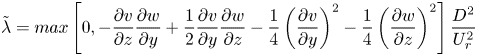 \begin{equation} \tilde{\lambda} = max\left [ 0, -\frac{\partial v}{\partial z} \frac{\partial w}{\partial y} + \frac{1}{2}\frac{\partial v}{\partial y} \frac{\partial w}{\partial z} - \frac{1}{4} \left ( \frac{\partial v}{\partial y} \right )^{2} - \frac{1}{4} \left ( \frac{\partial w}{\partial z} \right )^{2} \right ]\frac{D^2}{U_r^2} \end{equation}
from each of the vector fields measured using PIV. The  $\tilde {\lambda }$ fields were then time-averaged to produce the subplots of figure 3. Note in figure 3 that bands of high $\overline {\tilde {\lambda }}$ also coincide with bands of low $\overline {\tilde {U}}_{v,w}$ in figure 2, attesting to the vorticity that develops along the mixing interface.
Mean swirl strength  $\overline {\tilde {\lambda }}$ distributions with streamlines of in-plane velocity in overlay. (a) Case $eq_1$, (b) case $eq_2$, (c) case $lo_1$, (d) case $lo_2$, (e) case $hi_1$, ( f) case $hi_2$. Left-hand panels show data for the equal velocity cases ( $V_{rt} = 1$), whereas the right-hand panels present findings for the slower left-hand channel cases ( $V_{rt} =0.56$). Flow is into the page.
The highest values of  $\overline {\tilde {\lambda }}$ are collocated with the SOV cores identified by the streamline overlays in figure 3. The greatest $\overline {\tilde {\lambda }}$ occurs in $hi_{2}$ and to a lesser extent in $lo_2$ (the cases with a slower left channel). The tilted band of $\overline {\tilde {\lambda }}$ leading from the high values of $\overline {\tilde {\lambda }}$ near the bed in these cases, to the surface are caused by numerous vortices with diameters $\approx$ 0.1H often observed to descend from the surface, and down the mixing interface before eventually coalescing with the larger SOV cores. These vortices have a predominant clockwise sense of rotation and originate upstream in the confluence before momentarily being visualised as they advect through the laser sheet (see LIF movie 1 of $hi_{2}$ available at https://doi.org/10.1017/jfm.2023.656 (also available at https://youtu.be/aTqLrtxW9Wg)).
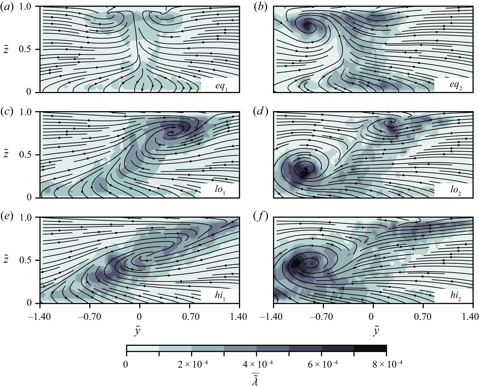
Dimensionless, two-component turbulent kinetic energy distributions ( $\tilde {k}_{v,w}$, right column figure 4) also coincide with zones of low $\overline {\tilde {U}}_{v,w}$ in figure 2. Notably, much of the in-plane kinetic energy is caused by the lateral fluctuations of the mixing interface due to passing episodic pulses. This is apparent by the greater contribution of dimensionless lateral kinetic energy ( $\tilde {k}_{v}$), compared with that of its vertical counterpart ( $\tilde {k}_{w}$) in figure 4. Generally, the contribution of $\tilde {k}_{w}$ is only significant near the SOV cores, indicating that over much of the mixing interface, $\tilde {k}$ is generated by the lateral fluctuations of the mixing interface.
Contours of dimensionless in-plane turbulent kinetic energy ( $\tilde {k}_{v,w}$, right) and its lateral ( $\tilde {k}_{v}$, left) and vertical ( $\tilde {k}_{w}$, middle) components for each of the six cases. Flow is into the page.
3.2. Instantaneous flow field
Interactions between the magnitude of  $\Delta \rho$ and $Mr_{D}$ are apparent in the space–time matrices of figure 5. The matrices were constructed from the first 20 s ( $\tilde {t}\leq 19.5$) of LIF images for each case. In postprocessing the images are ‘stacked’ in time, thresholded based on pixel intensities and then volumetrically rendered to give a depth perspective when viewed from above. For the $eq_1$ case ( $Mr_{D} = 1$, equal density, figure 5a), the passage of episodic pulses is apparent by the fluctuations of the partition line that sharply separates the illuminated waters (grey tones) of the right channel (bottom portion of each subplot) from the clear water of the left channel (removed by thresholding, top portion of each subplot). Evidence of episodic pulses is also apparent when $Mr_{D} = 3.3$ (figure 5b) and the partition line is observed to have shifted towards $\tilde {y} = -1$ because of the additional momentum of the right channel.
Space–time matrices derived from volumetric postprocessing of temporally stacked LIF images. The matrices depict the passage of coherent secondary flow structures through the 4 $D$ measurement plane in time. (a) Case $eq_1$, (b) case $eq_2$, (c) case $lo_1$, (d) case $lo_2$, (e) case $hi_1$, ( f) case $hi_2$.

The small density difference of 0.33 kg m $^{-3}$ has important effects on the turbulent secondary flow structure of the mixing interface. In the $lo_1$ case, the dense front of the right channel often extends to ${\approx }\tilde {y} = -1$, with the occasional near-bed wisps extending farther (figure 5c). A visible increase in the spatial coherence of the secondary flow structure is apparent when the velocity of the left channel is decreased ( $lo_2$, figure 5d). The increase in coherence is even more apparent when $\Delta \rho$ is doubled to 0.66 kg m $^{-3}$ in the $hi_2$ case (figure 5f). A strongly coherent streamwise-orientated vortex persistently passes through the LIF measurement plane in the $hi_2$ case, with the left-most limit of the SOV being well defined at ${\approx }\tilde {y} = -1.7$. This lateral limit occurs where the dense front is arrested (confined) by the converging lateral momentum of the left channel. This also occurs for the other density cases, albeit in a less spatiotemporally coherent manner. In all cases, the presence of episodic pulses is apparent by the temporal variations in the amplitude of the partition line in figure 5. However, the character of the pulses differs considerably between the cases, suggesting that interactions between density effects and $Mr_{D}$ influence how these pulses develop.
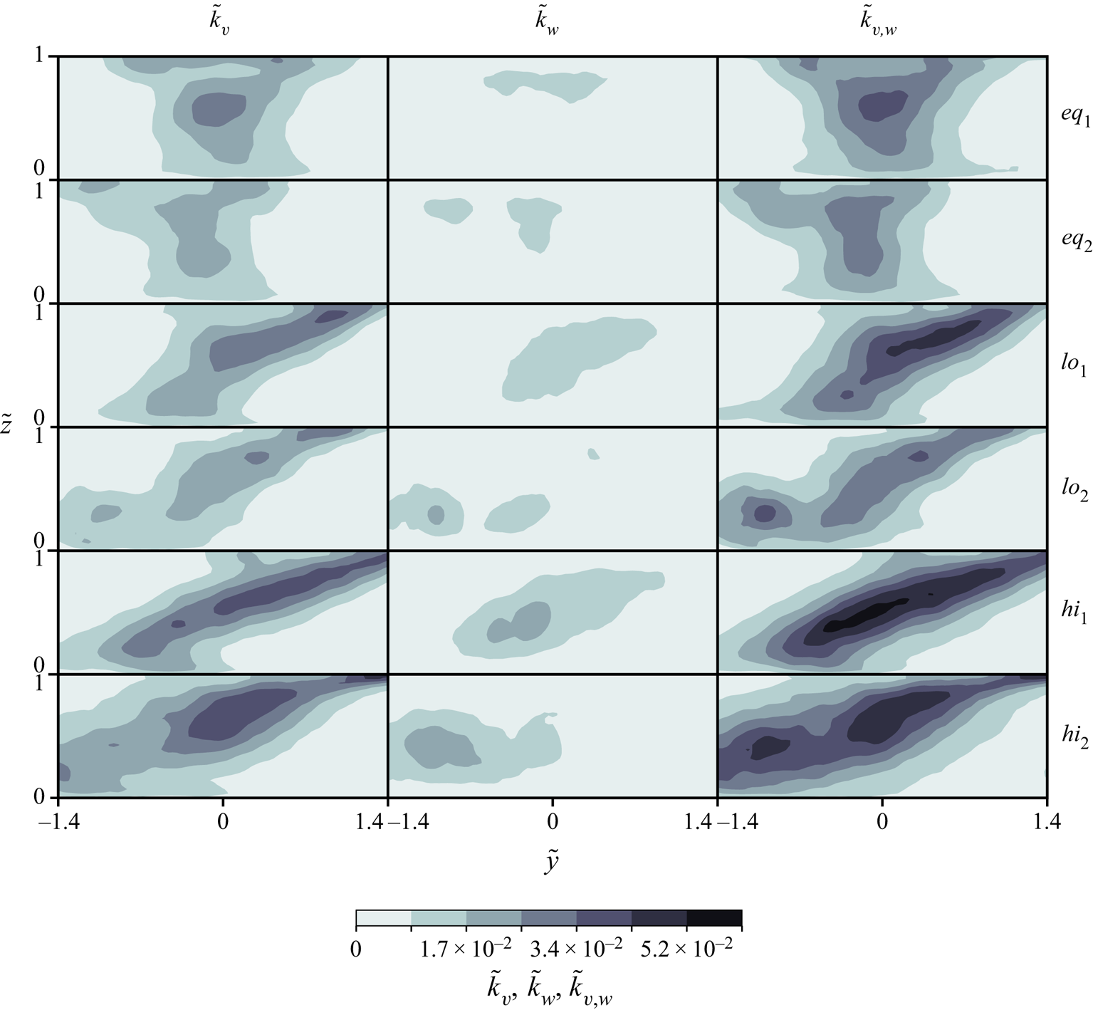
A sample time series of the instantaneous measurements on the  $\tilde {y}\tilde {z}$ plane are presented in figure 6. In the $eq_1$ case, the in-plane velocities on top of their corresponding LIF images reveal two counter-rotating, and nearly axisymmetric SOVs close to the free surface (figure 6a). These SOVs are confirmed to persist in time by the streamlines of average in-plane velocity (figure 2a). However, other vortical structures are also apparent in the water column that are not persistent in time. Their sense of rotation can be either clockwise or anticlockwise. Their presence averages out in figure 2(a), but their vorticity is apparent by the elevated values of $\overline {\tilde {\lambda }}$ in figure 3. In the $eq_2$ case a single anticlockwise rotating SOV appears near the surface, with other smaller vortices present below (figure 6b). The shift of the mixing interface towards the left is evident by its deviation from $\tilde {y} = 0.0$ to the left near the surface. This anticlockwise SOV also persists in the mean flow field (figure 2b).
Time series of the instantaneous flow structure with corresponding LIF images underlaid for the (a)  $eq_1$, (b) $eq_2$, (c) $hi_1$ and (d) $hi_2$ cases. Vector density has been decimated to improve clarity. Flow is into the page.
Numerous clockwise rotating instabilities develop along the mixing interface when the high-density difference is introduced and high velocities are present in the left channel (case  $hi_1$, figure 6c). These are instabilities generated by shear as the dense front attempts to move left, yet is opposed by the light channel as it is pulled above in the opposite direction due to the incompressibility constraint. The light front can attain instantaneous lateral velocities similar to the bulk velocity of the right channel ( $\overline {\tilde {U}}_{v,w} \approx 0.8$). The average effect of the shear caused by the fast-overtopping flow of the light channel is the nearly linear tilt of the mixing interface apparent in figure 2(e).
Despite cases  $hi_1$ and $hi_2$ having the same magnitude of $\Delta \rho$, their secondary flow structures are drastically different. In $hi_2$ the inertial attributes of the left channel favour the formation of large and spatiotemporally coherent clockwise SOVs to the left of $\tilde {y} = 0$ (figure 6d). The distinguishing feature of case $hi_2$ is its lower momentum in the left channel compared with $hi_1$. Without the shear associated with the characteristically high lateral velocities of the faster front in case $hi_1$ (i.e. near the surface in figure 6c), the upwelling of the dense front in case $hi_2$ is permitted to coherently rise towards the surface (in contrast to being sheared and advected downstream in $hi_1$). Simultaneously, a volume of clear water from the left channel slowly moves over the SOV as it proceeds to the right to replace the fallen volume of dense fluid. Where the light front encounters the dense channel, it downwells between the SOV and the main front of the dense channel. Combined, these movements produce a clockwise rotating SOV that advects down the mixing interface, consistent with the confined gravity current mechanism proposed by Duguay et al. (Reference Duguay, Biron and Lacey2022a).
3.3. Focus on cases  $hi_2$ and $hi_1$


The density SOVs of case  $hi_2$ dynamically interact with passing episodic pulses in the mixing interface. The LIF movie of the $hi_2$ case best conveys these dynamics (see LIF movie 1). In movie 1 the SOVs often attain their greatest coherence when the pulses reach their maximum displacement in the $-\tilde {y}$ direction. Conversely, the coherence of the SOVs diminishes most as the pulses recede to their maximum $+\tilde {y}$ location. A time series of LIF images extracted from movie 1 is presented in figure 7 to illustrate these dynamics. At $\tilde {t} = 0.0$, the upright portion of the mixing interface is at its maximum $+\tilde {y}$ position (i.e. short black arrow, figure 7) and a plume of partially mixed fluid with a clockwise sense of rotation extends over the $-\tilde {y}$ portion. One should bear in mind that what is recorded on the light sheet largely results from processes that occurred upstream a few moments earlier.
Exemplary time series of LIF images from the  $hi_{2}$ case showing the dynamics of the confined gravity current with the progression ( $\tilde {t} = 0.00$ to 0.2.19) and recession ( $\tilde {t} = 2.19$ to 3.65) of a lateral pulse through the mixing interface. The length of the black arrows conveys the lateral displacement of the mixing interface. Flow is into the page.
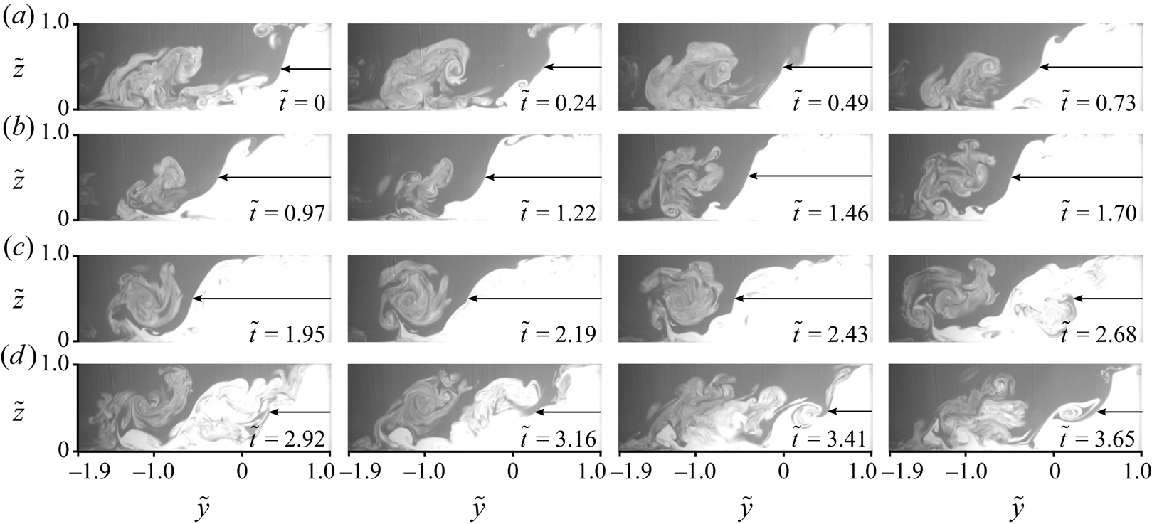
As time progresses from  $\tilde {t} = 0.00$, the pulse of dense fluid from upstream enters the light sheet progressively farther to the left. The coherence of the plume increases until a near-circular SOV forms (i.e. $\tilde {t} = 2.19$) as the crest of the pulse passes through 4 $D$. Then, as the trough proceeding the crest advects through the laser sheet, the mixing interface inclines and the SOV loses much of its coherence, causing a large number of smaller streamwise-orientated vortices to develop with a dominant clockwise sense of rotation. Importantly, between $\tilde {t} = 2.43$ and $\tilde {t} = 2.68$ the position of the mixing interface quickly shifts to the right (much shorter arrow). This happens because the passage from crest to trough abruptly occurs. Eventually, the sharp interface recedes to the maximum $+\tilde {y}$ position and the LIF image ( $\tilde {t} = 3.65$) resembles that at the beginning of the cycle. Over the course of the cycle, a layer of buoyant warm fluid persists above and to the side of the dense plume that remains at essentially the same lateral position (i.e. $\tilde {y}\approx -1.5$), despite the obvious lateral shifts of the mixing interface by $\Delta \tilde {y} \approx 1$. This lateral position is persistent and was also noted in the volumetric renders of figure 5( f).
Now a description of the flow as viewed on a LIF plane parallel to the bed and positioned at  $\tilde {z} = 0.5$. The flow in figure 8 has the same $hi_2$ conditions used in figure 7, but was measured on a different date. As in figure 7, figure 8 begins at $\tilde {t} = 0.00$, in the trough of the preceding pulse. As $\tilde {t}$ progresses, the crest of the pulse advances until it attains $\tilde {x} = 4$ (the location of the vertical light sheet used in figure 7) at ${\approx }\tilde {t} = 2.2$. This corresponds to when the adjacent SOV is most coherent (e.g. $\tilde {t} = 2.19$ in figure 7). As the pulse advances farther downstream, the interface at 4 $D$ gradually moves to the right until the second trough (appearing at $\tilde {t} = 2.48$) passes through 4 $D$ at ${\approx }\tilde {t} = 4.13$. This corresponds to when the coherence of the SOVs is least (i.e. $\tilde {t} = 0.00$ and 3.65 in figure 7).
The LIF experiment showing a plane parallel to the bed positioned at  $\tilde {z} = 0.5$ (flow is from left to right in each subplot). From top left to bottom right, a single period of a lateral pulse from trough to trough in the $hi_2$ case is shown as the pulse progresses down the mixing interface. Lighter tones indicate dense fluid from the right channel. Partially mixed patches in the upper half of the images correspond to upwelling of denser fluid within streamwise-orientated vorticity. Note that banding is caused by light refracting on the interfaces between the two fluids.

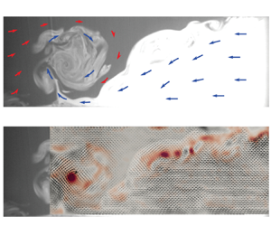
The flow in the vicinity of the density SOVs is conceptualised in figure 9(a) and supported by the measured vectors in figure 9(b). The cold dense front deflects upwards upon contact with the opposing water of the left channel ( $\tilde {y}\approx -1.5$ in figure 9). A portion of the buoyant flow from the left channel then flows over the deflected dense front, towards the partition line near the surface. This causes the dense front to curl over itself and a portion of warm fluid to be trapped between the SOV and the main body of dense flow. Because this happens simultaneously over a sizeable portion of the mixing interface, the result is a rolled-up and volumetrically coherent density SOV advecting downstream. The contours of non-dimensional vorticity
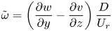 \begin{equation} \tilde{\omega}=\left(\frac{\partial w}{\partial y}-\frac{\partial v }{\partial z} \right )\frac{D}{U_r} \end{equation}
in figure 9(b) indicate the strength and clockwise sense of rotation of the large density SOV to the left and the smaller streamwise vortices often observed descending the mixing interface (see movie 1).
Turbulent mixing interface with a coherent density SOV. (a) A LIF image from the  $hi_{2}$ case showing the cross-section of a large diameter density SOV ( $\varnothing \approx 0.8D$) confined between the lighter, slower flow on the left, and the denser, faster flow on the right. Arrows show typical flow patterns in the vicinity of the SOV. (b) Vectors of instantaneous in-plane velocity ( $\tilde {U}_{v,w}$) over contours of $\tilde {\omega }$. The turbulent structure of the LIF is revealed by making the vector image overlay partially transparent. The left-most portion of the vector field was beyond the field of view of the PIV and, therefore, not measured. Flow is into the page.

The secondary flow structure in the mixing interface is much different in the  $hi_1$ case. The effects of the higher inertia of the left channel on the turbulent secondary flow structure are apparent by comparing LIF time series from $hi_1$ in figure 10 with those of $hi_{2}$ in figure 7 (see movie 2 (also available at https://youtu.be/h75POhbmm6Y)) for LIF of $hi_1$ case). First, a persistent tilt of the mixing interface consistent with the mean flow field depicted in figure 2(e) is noted. Second, and importantly, the diameter of the secondary flow cell is smaller now due to the fast buoyant flow of the left channel moving quickly above. Third, a greater volume of fluid above the dense front is occupied by that of the left channel. Finally, the mixing interface is characterised by many small diameter interfacial vortices resulting from considerable shear along the gravitationally adjusted mixing interface.
Exemplary time series of LIF images from the  $hi_1$ case showing the dynamics of turbulent secondary flow features in the mixing interface over the same time interval as in figure 7. Flow is into the page.

The flow field of the  $hi_1$ case is conceptualised in figure 11(a), and supported by measured velocity vectors in figure 11(b). Small diameter density SOVs develop where the dense front is arrested by the lateral momentum of the left channel. These are also more ephemeral than the large density SOVs of the $hi_2$ case (comparing movie 1 and movie 2), as they are more quickly advected downstream. The mixing interface also presents numerous streamwise KH vortices at mid-depth and higher, which in contrast to $hi_2$, are observed to ascend, rather than descend the mixing interface. The greater inertia of the light channel sweeps above the dense front, shearing it and generating these streamwise KH vortices.
Turbulent flow field of the mixing interface with small diameter density SOVs and numerous ascending streamwise-oriented KH vortices. (a) A LIF image from the  $hi_1$ case with numerous interfacial instabilities and a small diameter ( $\varnothing \approx 0.4D$) density SOV at the tip of the dense front. Arrows conceptualise flow patterns. (b) Vectors of $\tilde {U}_{v,w}$ are placed above contours of $\tilde {\omega }$. The left-most portion of the vector field was beyond the field of view of the PIV and therefore not measured. Flow is into the page.

3.4. Instantaneous circulation analysis
Vortex circulation ( $\varGamma$) is a useful metric to examine how each flow condition affects the strength and dominant sense of rotation of the secondary flow structures in the mixing interface. The $\varGamma$ of a vortex, such as an SOV traversing the 4 $D$ plane, can be calculated as the line integral of $\boldsymbol {U}_{v,w}$ tangent to the circumference of the vortex ( $\boldsymbol {L}$),
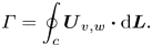 \begin{equation} \varGamma = \oint_{c} \boldsymbol{U}_{v,w}\boldsymbol{\cdot} {\rm d}\boldsymbol{L}.\end{equation}
However, Stokes’ theorem allows a more convenient calculation of  $\varGamma$ as the surface integral of $\omega$ over the vortex area ( $\boldsymbol {S}$),
 \begin{equation} \varGamma = \int_{S} \left ( \frac{\partial w}{\partial y}-\frac{\partial v }{\partial z} \right ) \boldsymbol{\cdot} {\rm d}\boldsymbol{S} = \int_{S} \omega \boldsymbol{\cdot} {\rm d}\boldsymbol{S} \end{equation}
and non-dimensionalized as
 \begin{equation} \tilde{\varGamma} = \frac{\varGamma}{DU_{r}}. \end{equation}
 For our purpose, the cross-sectional area of a vortex on the PIV plane is a detached region of  $\tilde {\lambda }>0$ (dark shades in figure 12, step 3). The integral of $\tilde {\omega }$ within this region is an estimate of that vortices’ circulation ( $\tilde {\varGamma }$), with positive $\tilde {\varGamma }$ indicating anticlockwise rotation, denoted and calculated as
 \begin{equation} \tilde{\varGamma}_{\curvearrowleft}=\tilde{\varGamma} > 0 \end{equation}
and negative  $\tilde {\varGamma }$ indicating clockwise rotation, denoted and calculated as,
 \begin{equation} \tilde{\varGamma}_{\curvearrowright}=\tilde{\varGamma} < 0. \end{equation}
Masking of a vorticity field using swirl strength and then its dissection to identify clockwise and anticlockwise vortices necessary for calculating  $\varGamma$.

The steps necessary to mask the vorticity field of the  $hi_2$ case based on $\tilde {\lambda }$ and its subsequent dissection into clockwise and anticlockwise rotating vortices is depicted in steps 2–6 in figure 12. At any given instant, many SOVs, possibly with an opposing sense of rotation, are often observed to comprise a larger secondary flow structure (see figure 12), thus making attempts to calculate the circulation of individual density SOVs difficult. However, the total circulation of all anticlockwise vortices,
 \begin{equation} sum(\tilde{\varGamma}_{\curvearrowleft})= \sum_{i=1}^{N}\tilde{\varGamma}_{\curvearrowleft}, \end{equation}
and the total circulation of all clockwise vortices,
 \begin{equation} sum(\tilde{\varGamma}_{\curvearrowright})=\sum_{i=1}^{N} \tilde{\varGamma}_{\curvearrowright}, \end{equation}
can be readily calculated to provide convenient metrics to examine how a flow condition influence's the mixing interface's secondary flow structure.
3.4.1. Instantaneous $sum(\tilde {\varGamma })$ analysis

As depicted in figure 13(a), the time series of  $sum(\tilde {\varGamma }_{\curvearrowleft })$ and $sum(\tilde {\varGamma }_{\curvearrowright })$ for the equal density and $Mr_{D} = 1$ $eq_1$ case are, as expected, of similar magnitude ( $|sum(\overline {\tilde {\varGamma }_{\curvearrowleft }})| = 0.70$, $|sum(\overline {\tilde {\varGamma }_{\curvearrowright }})| = 0.63$, with bars indicating absolute values as clockwise $\tilde {\varGamma }$ is negative). The anticlockwise SOVs appearing near the surface in case $eq_{2}$ (see figures 3(b) and 6(b)) explain why the anticlockwise circulation is generally greater than the clockwise circulation in figure 13(b) ( $|sum(\overline {\tilde {\varGamma }_{\curvearrowleft }})| = 0.88$ compared with $|sum(\overline {\tilde {\varGamma }_{\curvearrowright }})| = 0.57$, respectively).
Time series of  $sum(\tilde {\varGamma })$ for the six studied cases. Left-hand panels show data for the equal momentum ratio cases ( $Mr_{D} = 1$), whereas the right-hand panels present findings for the high momentum ratio cases ( $Mr_{D} = 3.3$). As clockwise circulation is negative by definition, absolute values are presented for comparative purposes.

Introducing a  $\Delta \rho$ of 0.33 kg m $^{-3}$ in $lo_{1}$ causes a clockwise dominant secondary flow structure to develop (figure 13c), with $|sum(\overline {\tilde {\varGamma }_{\curvearrowright }})| = 1.14$ being 1.8 times greater than $|sum(\overline {\tilde {\varGamma }_{\curvearrowleft }})|$ of 0.65. Interestingly, increasing the momentum ratio has a counteracting effect on total circulation, where the anticlockwise circulation in case $eq_2$ counteracts the stronger clockwise effects of density, thus reducing the dominance of clockwise secondary flow structures in case $lo_2$ compared with $lo_1$ (figure 13d). Therefore, the effects of $\Delta \rho = 0.33$ kg m $^{-3}$ on $|sum(\overline {\tilde {\varGamma }_{\curvearrowright }})|$ are less pronounced between $eq_2$ and $lo_2$ than they are between $eq_1$ and $lo_1$.
Increasing  $\Delta \rho$ further to 0.66 kg m $^{-3}$ in $hi_{1}$ (figure 13e) developed a mixing interface clearly dominated by clockwise vorticity, with a $|sum(\overline {\tilde {\varGamma }_{\curvearrowright }})|$ of 1.6, or a factor 2.1 times greater than $|sum(\overline {\tilde {\varGamma }_{\curvearrowleft }})|$ of 0.75. In the $hi_1$ case, clockwise circulation is a factor 2.6 times stronger than in $eq_1$. With a larger density difference, the counteracting effect of $Mr_{D}$ is reduced, so clockwise circulation clearly dominates in both $hi_1$ and $hi_2$ (figure 13e, f). Such additional clockwise circulation caused by density differences is expected to significantly increase mixing rates. Pronounced periodic peaks are also observed in the time series of figure 13( f) and are the subject of the next section.
3.4.2. Instantaneous $Hi_{2}$ circulation

The LIF movie of case  $hi_2$ shows strong lateral incursions (movie 1). The peaks in $sum(\tilde {\varGamma })$ in figure 13( f) are correlated to these incursions. A metric was derived from the LIF movie frames to assess these correlations. First, the LIF frames were cropped to define a sampling surface spanning a $\Delta \tilde {y}$ range of 0.5 on both sides of $\tilde {y} = -0.29$ ( $-$0.29 is $\approx$ the centre of the laterally shifted mixing interface caused by the greater $Mr_{D}$ of the $eq_2$ case; see figure 3b). The LIF images were binarized at an appropriate threshold intensity to make pixels containing fluoresced dye equal to 1 and those without dye equal to 0. Equation (3.10) was then applied to calculate $sum(I)$
 \begin{equation} sum(I)=\frac{1}{M*N}\sum_{i=1}^{M}\sum_{j=1}^{N} I_{i,j} \end{equation}
(where  $M$ and $N$ are respectively the number of rows and columns of pixels in the cropped image). A time series of the resulting $sum(I)$ is presented in figure 14(a). The mean of $sum(I)$ is 0.52, indicating the LIF sampling zone was approximately centred about the lateral fluctuation point.
Non-dimensionalized time series: (a)  $sum{(I)}$, (b) non-dimensionalized lateral velocity spatially averaged over the top half of the LIF sampling zone, (c) clockwise (blue) and anticlockwise (red) circulation $sum(\tilde {\varGamma })$.

The peaks in  $sum(I)$ occur when the lateral pulses are farthest to the left, therefore occupying a majority of the sampling zone. This is also when the lateral flow is predominantly negative (i.e. the pulse of dense fluid is moving towards the left, see figure 14(b), where $\sigma _{v}$ is the standard deviation of $\tilde {v}$). In contrast, the peaks in the $|sum(\overline {\tilde {\varGamma }})|$ generally lag those of $sum(I)$ (vertical lines help compare figure 14a,c). Observation of the LIF movie in conjunction with movies of the vorticity field, shows vorticity attains its maximum as the pulse of dense fluid recedes towards the right. As it recedes, the spatially averaged velocity in the top half of the LIF sampling region (i.e. $\tilde {z}>0.5$) becomes strongly positive (i.e. the upper portion of the water column is moving to the right). The peaks in circulation result as numerous smaller interfacial vortices develop due to shear as lighter fluid is pulled over the gravity current as the pulse recedes.
Cross-correlation analysis between  $sum(I)$ and $\tilde {\varGamma }_{\curvearrowright }$ using
 \begin{equation} R_{\sigma_I\tilde{\varGamma}_{\curvearrowright}} = \frac{\displaystyle\frac{1}{N}\sum_{n=1}^N I(n) \tilde{\varGamma}_{\curvearrowright}(n+\Delta\tilde{t})}{\sigma_I \sigma_{\tilde{\varGamma}_{\curvearrowright}}}, \end{equation}
where  $\Delta \tilde {t}$ is the non-dimensionalized time lag, shows a peak at $\Delta \tilde {t} = 0.62$ (figure 15), in agreement with observed lags between peaks of $sum(I)$ and $sum(\tilde {\varGamma })$ in figure 14.
Cross-correlation of  $sum(I)$ with $\tilde {\varGamma }_{\curvearrowright }$ and autocorrelation of $\tilde {\varGamma }_{\curvearrowright }$.

Finally, auto-correlations of  $sum(I)$ using
 \begin{equation} R_{\tilde{\varGamma}_{\curvearrowright}\tilde{\varGamma}_{\curvearrowright}} = \frac{\displaystyle\frac{1}{N}\sum_{n=1}^N \tilde{\varGamma}_{\curvearrowright}(n) \tilde{\varGamma}_{\curvearrowright}(n+\Delta\tilde{t})}{\tilde{\varGamma}_{\curvearrowright} \tilde{\varGamma}_{\curvearrowright}} \end{equation}
produce a peak at 3.3  $\Delta \tilde {t}$ (figure 15) indicating lateral pulses visible in the LIF movie occur at a dimensionless frequency of 0.30 (calculated as $1/\Delta \tilde {t}$). This frequency was also corroborated by peaks in power spectral density plots of $sum(I)$ and $\tilde {v}/\sigma _{\tilde {v}}$ (not shown).
4. Discussion
Density differences are likely always present to some degree at natural river confluences. Therefore, understanding how they affect secondary flow is necessary if confluence hydrodynamics is to be understood. Our experiments, performed in a laboratory confluence allowing a thermal difference between its tributaries, reveal quite clearly how the magnitude of  $\Delta \rho$ interacts with the inertia of the tributaries to alter confluence hydrodynamics. The spatiotemporal resolution of our data has permitted a number of insights into these processes.
A key finding is that density SOVs, similar to those observed at the Coaticook- Massawippi confluence can be reproduced empirically. Several shared traits were noted between the density SOVs of case  $hi_2$ and those of the Coaticook-Massawippi confluence, and this despite the nearly two-order magnitude difference in physical scale of these confluences (postconfluent widths of 0.5 and 34 m, respectively). For instance, in both the lab and field confluences, the density SOVs dynamically interact with passing episodic pulses, revolve clockwise around the streamwise axis and increase in coherence as the episodic pulses push farther into the light channel. Furthermore, remarkable similarities are often observed in the instantaneous cross-sections of their mixing interfaces. Figure 16 shows a collection of qualitative matches of their flow structures (scaled by the mixing interface depth). Cross-sections in the right-hand column of figure 16 are taken from the numerical model of the Coaticook-Massawippi confluence of Duguay et al. (Reference Duguay, Biron and Lacey2022a). The red fluid is the denser Coaticook that was modelled to be 0.5 kg m $^{-3}$ denser than the Massawippi (blue). The interested reader is directed to Duguay et al. (Reference Duguay, Biron and Lacey2022a) for full details on the model's parameters. The similarities apparent in figure 16 suggest the confined gravity current is a scale-independent secondary flow pattern at confluences.
The LIF visualisations of density-driven secondary flow structures in the  $hi_2$ case (left panels) with similar flow structures (right panels) in the eddy-resolved $\alpha$ contours (mixed density field, useful to observe secondary flow structures, see Duguay et al. Reference Duguay, Biron and Lacey2022a) modelled at the Coaticook-Massawippi confluence. The numerical panels are from the $\overleftarrow {\Delta \rho }_{0.5}$ eddy-resolved numerical simulation of Duguay et al. (Reference Duguay, Biron and Lacey2022b) (see their figure 3 for cross-section location). The depth in the centre of the cross-section (1.6 m) was used to non-dimensionalize $y$ for the Coaticook-Massawippi confluence. Resemblances: (a) a pulse receding to the right, (b) a pulse advancing to the left, (c) dense front extending left and (d) smaller KH instabilities descending the mixing interface.

4.1. Conceptual description of three-dimensional density-driven flow at confluences
Our results taken on a single cross-section show that density gradients strongly alter the secondary flow structure. However, what remains challenging is to understand the complex three-dimensional (3-D) dynamics of the confined gravity current, a difficult task given the inherent limitations of our planar PIV methodology. Nevertheless, these dynamics can be observed directly in the laboratory and an attempt is made here to convey them by discussing plan-view movies of the  $hi_2$ 3-D flow field as revealed by a fluorescent black-light imaging technique (see movie 3 (also available at https://youtu.be/yhJQ0u5UZHk)). Similar to the LIF measurements, fluorescein dye was mixed in the right channel. However, in the left channel a stream of fluorescent dye was injected 1 cm below the surface near the wall upstream of the apex allowing it to be visualised as it mixed within the density SOV. The dye was fluoresced using two 50 W LED black lights positioned above the flume. Figure 17 presents a time series of still images extracted from movie 3 to illustrate key events and their locations in the mixing interface.
Still images taken from the dye visualisation movie of the  $hi_2$ case (movie 3). An injected stream of fluorescent dye is tracked as it first downwells ( $\tilde {t} = 2$), laterally advects within the density SOV close to the bed ( $\tilde {t} = 4$), upwells towards the surface ( $\tilde {t} = 6$), laterally advects towards the dense channel ( $\tilde {t} = 8$) before finally downwelling a second time ( $\tilde {t} = 10$) to complete a revolution. The bright line indicates the centre of the flume ( $\tilde {y} = 0$), whereas the numbers indicate intervals of $D$ downstream. Here $\tilde {t} = 0$ is arbitrarily defined for illustration purposes and is not related to the start of movie 3.

As flow enters the confluence, it separates from the edges of the observation window (forming the stagnation zone) before colliding at  $\approx 2D$ (left in subplots of figure 17). Upon collision, the horizontal shear generates vertically orientated KH instabilities that deform and stretch laterally as the dense side of the mixing interface slumps along the bed (indicated in figure 17, and visible to some extent in movie 3). Between distances of 1 $D$ and 2 $D$, the density difference is strongest and considerable slumping is observed. Following a stream of injected dye through time, beginning at $t = 0$ s in figure 17, the dye crosses laterally to the right above the slumping dense front (due to the incompressibility constraint) before downwelling upon contact with the opposing dense channel (figure 17 $\tilde {t} = 2$). In movie 3 the downwelling dye is often observed to mix within vertically orientated KH instabilities (indicated in the bottom right panel of figure 17) before laterally advecting along the bed ( $\tilde {t} = 4$). The dense front, now carrying the stream of injected dye, upwells and is sheared back towards the dense channel ( $\tilde {t} = 6$) as a portion of the light channel is pulled above the SOV ( $\tilde {t} = 8$). Once near the dense channel, the dye downwells a second time to complete a full revolution about the streamwise axis ( $\tilde {t} = 10$). This revolution occurs over a distance of $\tilde {x}\approx 7.14$ in $\tilde {t}\approx 7.5$, for an approximate revolution rate of 0.84 rad $\tilde {t}^{-1}$. By the time the injected dye attains $\tilde {x} = 9D$, it is generally well mixed and difficult to discern.
On some occasions in movie 3, highly coherent density SOVs form resembling those observed and discussed by Duguay et al. (Reference Duguay, Biron and Lacey2022a). The production of secondary circulation and the coherence of the density SOV appears to be greatest where the flows encounter one another with greatest opposing momentum (i.e. between 1 $D$ and 4 $D$). Also, the SOVs and KH instabilities (episodic pulses) grow laterally and stretch longitudinally as flow accelerates into the postconfluent reach. These dynamics are all similar to those of the SOV observed and described in the Coaticook-Massawippi confluence. Figure 18 conceptualises the key density-driven secondary flow patterns applicable to the laboratory confluence. Based on the similarities with the Coaticook-Massawippi case, the conceptual patterns should equally apply to many natural confluences.
Conceptualisation of the density-driven secondary flow patterns at river confluences based on observations in movie 3 of the  $hi_2$ case. The depicted flow patterns are proposed to be scale independent, as similar patterns were noted at the Coaticook-Massawippi confluence by Duguay et al. (Reference Duguay, Biron and Lacey2022a).

4.2. Secondary flow structure without density effects
As expected, the mixing interfaces of the  $eq_1$ and $eq_2$ cases were nearly vertical. However, dual back-to-back surface-convergent SOVs, which have been largely attributed to, or at least discussed in relation to the downwelling of superelevated flow (Mosley Reference Mosley1976; Ashmore Reference Ashmore1982; Paola Reference Paola1997; Constantinescu et al. Reference Constantinescu, Miyawaki, Rhoads, Sukhodolov and Kirkil2011; Sukhodolov & Sukhodolova Reference Sukhodolov and Sukhodolova2019), did not develop in either $eq_1$ or $eq_2$. Instead, two small, surface-divergent SOVs developed near the surface, rotating in the opposite sense to that predicted if downwelling superelevated flow was their cause. Injected dye visualisations showed these vortices originate at the downstream tip of the stagnation zone between $\approx$1 $D$ and 2 $D$ (see injected dye visualisations of case $eq_1$ in movie 4 (also available at https://youtu.be/_OYi3qJQv6w). They develop as the flow carrying the injected dye is deflected upwards upon colliding with the flow of the right channel. Then, trapped between the free surface and the ambient flow, the deflected flow becomes confined within a spiraling SOV.
In movie 4 the coherence of these SOVs is greatest when the dye stream hits an advancing episodic pulse from the right channel (i.e. hits the side of a pulse moving into the left channel). However, if the dye stream instead enters when the pulse is receding, the collision is less abrupt and much of the left channel's momentum smoothly advects downstream, with notably less streamwise vorticity being produced. By the principle of the conservation of momentum, we presume that as the fluid carrying the dye stream abruptly collides with an advancing pulse, a portion of its momentum converts into the angular momentum of the SOV during the collision. This is a plausible explanation for the coherent SOVs measured near the surface in figure 3(a) (and observed directly in the laboratory dye visualisations), yet requires empirical validation.
A similar momentum conversion mechanism is also proposed to result in the lone anticlockwise SOVs rotating near the surface in the  $eq_2$ case (see figure 2(b) and movie 5 (also available at https://youtu.be/LHVPRA8NfG0)). Interestingly, similar lone anticlockwise SOVs were also noted in the mixing interface of the equal density simulation of the Coaticook-Massawippi confluence of Duguay et al. (Reference Duguay, Biron and Lacey2022b) (see their figure 3d) and in situ at the Coaticook-Massawippi confluence when there was no density difference between the tributaries (see figure 10 Duguay et al. Reference Duguay, Biron and Lacey2022b). Though many details of how these anticlockwise near-surface SOVs form are lacking, their presence at the Coaticook-Massawippi confluence and in the laboratory suggests they may be common coherent flow structures at confluences, irrespective of the confluence's physical scale. Further research on this topic is required.
4.3. The densimetric Froude number
The effect of density gradients on a confluence's hydrodynamics is typically parameterised using the densimetric Froude number ( $\boldsymbol {F}_{D}$),
 $$\begin{gather} \boldsymbol{F}_{D} = \frac{U_{0}}{\sqrt{g'D}}, \end{gather}$$
 $$\begin{gather}g'=\frac{(\rho_{1}-\rho_{2})}{\rho_{1}}g, \end{gather}$$
where  $g'$ is reduced gravity ((4.2) with $g$ the constant of gravitational acceleration, and $\rho _{1}$ and $\rho _{2}$ respectively the densities of the denser and lighter tributaries), $D$ is a characteristic depth and $U_{0}$ is a characteristic velocity (Rhoads Reference Rhoads2020). However, Duguay et al. (Reference Duguay, Biron and Lacey2022a) demonstrated that $\boldsymbol {F}_{D}$ can vary considerably depending on the definition of $D$ (e.g. average cross-sectional main channel depth, average cross-sectional tributary depth, average depth in the mixing interface) and $U_{0}$ (e.g. a discharge-weighted average of the tributaries’ bulk velocities, the bulk velocity of the tributary or the bulk velocity of the main channel). Also, Duguay et al. (Reference Duguay, Biron and Lacey2022b) showed that $\boldsymbol {F}_{D}$ is incapable of accounting for the effects that the sign of the density gradient has on secondary flow structure (i.e. a fast denser channel encountering a slow light channel produces different structures than a fast-light channel encountering a slow-dense channel). Because of this variability and because there is currently no consensus on which values of $D$ and $U_{0}$ should be used, we have deliberately avoided referring to our trials in terms of $\boldsymbol {F}_{D}$.
Our experiments help further illustrate the difficulties encountered in defining  $\boldsymbol {F}_{D}$ as pointed out in Duguay et al. (Reference Duguay, Biron and Lacey2022a,Reference Duguay, Biron and Laceyb). Table 3 presents the values of $\boldsymbol {F}_{D}$ for each case with $U_0$ taken as either the cross-sectional average velocity of the left channel ( $U_l$), the right channel ( $U_r$) or the downstream channel $U_{dwn}$. Depending on which value of $U_0$ is taken, the same condition could have three possible values of $\boldsymbol {F}_{D}$. For example, $hi_2$ can be either 1.85, 3.35 or 4.17. Furthermore, different cases with disparate secondary flow patterns can nevertheless have an identical value of $\boldsymbol {F}_{D}$ depending on which definition of $U_0$ is used (e.g. $lo_1$'s value of 4.74 based on $U_{l}$ and $lo_2$'s value of 4.74 based on $U_{r}$, see patterns in figure 3). Also, if $U_{dwn}$ is used to define $U_{0}$ for case $lo_1$, then $\boldsymbol {F}_{D} = 7.58$, which many would agree should indicate insignificant density effects. Yet, the difference between the secondary flow patterns for cases $eq_1$ and $lo_1$ in figure 3 are by no means insignificant. Furthermore, the counteracting effect of velocity (or momentum) ratio and density difference on total SOV circulation (observed in figure 13) cannot be accounted for in the current definition of $\boldsymbol {F}_{D}$. It is not clear how to remove the ambiguities inherent to the use of $\boldsymbol {F}_{D}$ at confluences. However, the difficulties described here, in addition to those discussed by Duguay et al. (Reference Duguay, Biron and Lacey2022a,Reference Duguay, Biron and Laceyb), strongly suggest another metric is required so that density effects on confluence hydrodynamics can unambiguously be quantified. Future research effort on this topic is needed.
Densimetric Froude numbers considering three possible definitions of  $U_0$.
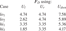
4.4. Other potential sources of secondary flow and future work
Our results provide compelling evidence that the observed secondary flow structures (i.e. SOVs) are caused by the gravitational adjustment of the mixing interface and its interaction with the converging ambient flows of the confluence. As the dense front slumps and begins to extend laterally, an equivalent volume of lower density fluid is pulled above due to the incompressibility constraint of water. The lateral movement of lower density fluid opposes that of the dense front and causes the dense fluid to curl above itself, thus initiating and maintaining streamwise-orientated vorticity. The strength of secondary circulation is a function of the hydrostatic pressure gradient between the tributaries (i.e.  $\Delta \rho gh$). As the pressure gradient increases, so does the speed of the slumping front and, consequently, that of the lighter fluid pulled above. The increase in the strength of circulation with increased $\Delta \rho$ noted herein (§ 3.4) supports this.
Curvature-induced secondary flow of Prandtl's first kind and turbulence-induced secondary flow from upstream (Prandtl's second kind) are not expected to contribute to the formation of the observed secondary flow structures (i.e. SOVs) in the density cases. If Prandtl's secondary motions of the first and second kind were important contributors, significant SOVs would have also been detected in the equal density cases. It is possible, however, that curvature-induced secondary flow may have more of an impact at meander-bend confluences such as the Coaticook-Massawippi confluence – the natural confluence studied in our previous work (Duguay et al. Reference Duguay, Biron and Lacey2022a,Reference Duguay, Biron and Laceyb). Yet, the fact that the coherent SOVs measured in our laboratory confluence of relatively mild curvature were so like those observed at the Coaticook-Massawippi meander-bed confluence of very pronounced curvature, suggests planform curvature and turbulence-induced secondary flow are of much less importance compared with the difference in density.
Though our results support density differences as being the main cause of the observed secondary flow, density effects do not act alone. The gravitationally adjusted mixing interface is also dynamically coupled to vertically orientated KH instabilities caused by lateral shear between the converging streams. The coherence of the SOVs is also altered by the momentum ratio of the confluence, with the SOVs being most coherent when a higher momentum denser channel collides with a lower momentum lighter channel. Furthermore, the average velocity of the flow through the confluence is also expected to alter the SOVs, as faster flows will result in shorter transit times of the fluid through the confluence and, consequently, less time for the denser fluid to slump laterally before being swept downstream. Finally, the sign of the density gradient is also expected to alter secondary flow production. A fast-light channel colliding with a slow-dense channel has been shown to produce a different secondary flow structure than a fast-dense channel colliding with a slow-light channel (Duguay et al. Reference Duguay, Biron and Lacey2022b). In the end, the relevant spatiotemporal scales of the density-driven secondary flow result from the complex interactions of a number of important hydrodynamic parameters of the confluence. Given this complexity, much additional research is required before density-driven secondary flow is to be fully understood and a means can be obtained to accurately predict mixing rates of two converging rivers.
5. Conclusions
Large diameter ( $\approx$0.8H) and strongly spatiotemporally coherent density SOVs were confirmed in a laboratory flume confluence designed to study thermally induced $\Delta \rho$ effects on secondary flow structure. The measured density SOVs share many similarities to the SOVs filmed in situ using an aerial drone at the natural Coaticook-Massawippi confluence by Duguay et al. (Reference Duguay, Biron and Lacey2022a). Measured flow fields, LIF and supporting fluorescent dye movies of the mixing interface show that the confined gravity current mechanism proposed by Duguay et al. (Reference Duguay, Biron and Lacey2022a) causes the density SOVs in the laboratory. The findings support the use of laboratory experiments in studying confluence hydrodynamics as they permit the application of spatiotemporally resolved flow field quantification and visualisation techniques that are currently not available in situ.
A main finding is that the inertia of the lighter tributary shears the dense front, and depending on the magnitude of this shear, it can either produce strongly coherent density SOVs as a portion of the light channel's flow gently moves over the dense front (e.g.  $hi_{2}$), or it can produce a tilted mixing interface replete with numerous streamwise-orientated KH instabilities as a portion of the light channel's flow rapidly moves over the dense front and shears the mixing interface ( $hi_1$). Greater bulk velocities through the confluence are proposed to sweep the protruding dense front downstream quicker, reducing the time available for the front to propagate laterally and develop into a large spatially coherent density SOV. Our work empirically shows the role of the confined gravity current mechanism in the formation of density SOVs such as those observed at the Coaticook-Massawippi confluence by Duguay et al. (Reference Duguay, Biron and Lacey2022a). Much work remains to understand how more complex confluence planforms, bathymetries and bed roughness alter confluence mixing interface dynamics subjected to $\Delta \rho$. Testing a larger range of velocity/momentum ratio conditions will also allow a better understanding of the interactions between density and inertia effects at natural confluences and their impact on longitudinal mixing rates. Eddy-resolved numerical modelling should prove useful in this regard, as the highly transient and multidimensional character of the mixing interface is difficult to study using laboratory and in situ methods. It has been demonstrated that even small variations in density can have a considerable impact on the secondary flow characteristics of a confluence. These variations are commonplace in natural confluences, as a result of differences in the temperatures of the tributaries and their concentrations of suspended sediments and dissolved minerals. Consequently, it is essential that future confluence research take these variations into account to reach valid conclusions.
Supplementary movies
Supplementary movies are available at https://doi.org/10.1017/jfm.2023.656.
Acknowledgements
We would like to extend our gratitude to the Université de Sherbrooke for providing access to the hydraulics laboratory needed to carry out these experiments. The comments of two anonymous reviewers are greatly appreciated.
Funding
The authors would like to thank the Fonds de Recherche du Québec - Nature et Technologies (FRQNT) for supporting the BX3 postdoctoral research scholarship that funded the majority of this research. The Natural Science and Engineering Research Council of Canada Discovery grant of P.M.B. and R.W.J.L. also supported this research.
Declaration of interests
The authors report no conflict of interest.


 Open access