


1. Introduction
The stability and laminar-to-turbulent transition of high-speed boundary layers have been extensively investigated in recent decades. The skin friction and heat flux can be escalated by several times after the transition is completed. As a result, the transition mechanism is of great significance. Physically, multiple processes can emerge during the instability and transition. From early to late stages, the physical processes may include the receptivity to external disturbances, transient growth, eigenmodal growth, parametric resonance and mode–mode interactions, breakdown to turbulence, etc. The specific transition path and involved process are dependent on the environmental disturbance level (Morkovin, Reshotko & Herbert Reference Morkovin, Reshotko and Herbert1994).
During the flight or in the quiet wind tunnel, the disturbance level tends to be relatively low. In this case, the long-distance eigenmodal amplification of small-amplitude disturbances is likely dominant in triggering the transition. Common boundary layer eigenmodes include the Tollmien–Schlichting mode in subsonic, the first mode in low supersonic, the Mack second mode in hypersonic boundary layers, etc. These modes are solvable from a local eigenvalue analysis. The terms ‘local’ and ‘global’ refer to the instability of the local profile and of the entire flow field, respectively (Huerre & Monkewitz Reference Huerre and Monkewitz1990). These local modes possess predominantly high growth rates of energy under certain conditions, and can be exponentially amplified (Mack Reference Mack1984; Fedorov Reference Fedorov2011). In contrast to the exponential growth, algebraic growth is also likely responsible for the transition. For instance, the eigenmodal growth can be bypassed, provided that the environment is sufficiently noisy. Another scenario is that the system is linearly stable by local normal-mode analysis, whereas it undergoes an evident algebraic growth from global analysis (Schmid Reference Schmid2007). The discrepancy is attributed to the fact that the global analysis can be based on the linearised Navier–Stokes (N–S) equation, which includes the non-normality nature of the operator. By contrast, a local analysis usually neglects this factor. From the perspective of local analysis, the growth of the convective instability is called ‘non-modal’ if the local normal-mode analysis reports no unstable solutions.
In the high-speed transition community, one of the issues under debate is the nose-tip bluntness effect, which may be linked with the non-modal growth discussed above. This bluntness effect arises as the leading edge of the vehicle needs to be blunted to mitigate aerodynamic heating. Historically, Stetson discovered the ‘transition reversal’ phenomenon due to the bluntness effect in different tunnel facilities (Stetson & Rushton Reference Stetson and Rushton1967; Stetson Reference Stetson1983). Later, this phenomenon has been widely reported by transition measurements over blunt flat plates (Lysenko Reference Lysenko1990; Borovoy et al. Reference Borovoy, Radchenko, Aleksandrov and Mosharov2022), blunt cones (Softley, Graber & Zempel Reference Softley, Graber and Zempel1969; Ericsson Reference Ericsson1988; Zanchetta Reference Zanchetta1996; Aleksandrova et al. Reference Aleksandrova, Novikov, Utyuzhnikov and Fedorov2014; Marineau et al. Reference Marineau, Moraru, Lewis, Norris, Lafferty, Wagnild and Smith2014; Paredes et al. Reference Paredes, Choudhari, Li, Jewell, Kimmel, Marineau and Grossir2019) and ogive cylinders (Hill et al. Reference Hill, Oddo, Komives, Reeder, Borg and Jewell2022) for a wide range of Mach numbers. To be specific, as the nose-tip bluntness (normally characterised by the radius) is gradually increased, the transition onset or end locations can be firstly delayed and then moved forward. These two distinct regimes, called the small-bluntness regime and the large-bluntness regime, display a reversal trend. The trend is usually observable in a $Re_{\textit {R}}$
–
$Re_{\textit {R}}$
– $Re_{\textit {t}}$
or
$Re_{\textit {t}}$
or $Re_{\textit {R}}$
–
$Re_{\textit {R}}$
– $Re_{\textit {T}}$
plot. Here,
$Re_{\textit {T}}$
plot. Here, $Re_{\textit {R}}$
,
$Re_{\textit {R}}$
, $Re_{\textit {t}}$
and
$Re_{\textit {t}}$
and $Re_{\textit {T}}$
refer to the Reynolds numbers based on the nose-tip radius, the transition onset location and the transition end location, respectively. More detailed introductions to the stabilisation effect of the entropy layer in the small-bluntness regime and to the poorly understood large-bluntness regime can be found in Part 1 (Guo, Hao & Wen Reference Guo, Hao and Wen2025). In addition to experimental research, numerical efforts on the receptivity (Zhong & Ma Reference Zhong and Ma2002, Reference Zhong and Ma2006; Kara, Balakumar & Kandil Reference Kara, Balakumar and Kandil2011; Balakumar & Kegerise Reference Balakumar and Kegerise2015; Balakumar & Chou Reference Balakumar and Chou2018; He & Zhong Reference He and Zhong2021; Ba, Niu & Su Reference Ba, Niu and Su2023) and the nonlinear instability stage (Paredes, Choudhari & Li Reference Paredes, Choudhari and Li2020; Hartman, Hader & Fasel Reference Hartman, Hader and Fasel2021; Goparaju & Gaitonde Reference Goparaju and Gaitonde2022; Liu et al. Reference Liu, Schuabb, Duan, Paredes and Choudhari2022; Zhu et al. Reference Zhu, Li, Guo, Liu and Tong2023) were also reviewed.
$Re_{\textit {T}}$
refer to the Reynolds numbers based on the nose-tip radius, the transition onset location and the transition end location, respectively. More detailed introductions to the stabilisation effect of the entropy layer in the small-bluntness regime and to the poorly understood large-bluntness regime can be found in Part 1 (Guo, Hao & Wen Reference Guo, Hao and Wen2025). In addition to experimental research, numerical efforts on the receptivity (Zhong & Ma Reference Zhong and Ma2002, Reference Zhong and Ma2006; Kara, Balakumar & Kandil Reference Kara, Balakumar and Kandil2011; Balakumar & Kegerise Reference Balakumar and Kegerise2015; Balakumar & Chou Reference Balakumar and Chou2018; He & Zhong Reference He and Zhong2021; Ba, Niu & Su Reference Ba, Niu and Su2023) and the nonlinear instability stage (Paredes, Choudhari & Li Reference Paredes, Choudhari and Li2020; Hartman, Hader & Fasel Reference Hartman, Hader and Fasel2021; Goparaju & Gaitonde Reference Goparaju and Gaitonde2022; Liu et al. Reference Liu, Schuabb, Duan, Paredes and Choudhari2022; Zhu et al. Reference Zhu, Li, Guo, Liu and Tong2023) were also reviewed.
Some of the 3-D simulation work can capture the flow structures that qualitatively resembled the experimental image (Hartman et al. Reference Hartman, Hader and Fasel2021; Liu et al. Reference Liu, Schuabb, Duan, Paredes and Choudhari2022). Nonetheless, no numerical simulation replicated the transition reversal phenomenon that agreed with the experiment. Recently, Guo et al. (Reference Guo, Hao and Wen2025) simulated the complete transition to turbulence over a blunt plate with varying nose-tip radii. The authors applied three-dimensional (3-D) broadband slow acoustic perturbations in front of the bow shock to trigger the instability and transition at Mach 5. A good agreement with the experimental $Re_{\textit {R}}$
–
$Re_{\textit {R}}$
– $Re_{\textit {t}}$
curve was achieved for the first time, which manifested the transition reversal.
$Re_{\textit {t}}$
curve was achieved for the first time, which manifested the transition reversal.
As a continuation question of Guo et al. (Reference Guo, Hao and Wen2025) where acoustic perturbations were utilised, the response of the flow over a largely blunted body to various types of free-stream disturbances merits an investigation. Basically, there are fundamental types of disturbances in the uniform free stream, namely slow/fast acoustic waves, vortical waves and entropy waves (Kovasznay Reference Kovasznay1953). They are independent solutions when the perturbation amplitude is small to allow the linearisation of the governing equation. Over configurations such as flat plates, wedges and cones, the instability waves in boundary layers are three to five times more susceptible to slow acoustic waves than fast acoustic, vorticity and entropy waves (Balakumar & Kegerise Reference Balakumar and Kegerise2015; He & Zhong Reference He and Zhong2022). Numerical and experimental studies have revealed that the slow acoustic wave dominates the environment of noisy hypersonic tunnel facilities (Laufer Reference Laufer1961; Schneider Reference Schneider2001; Wagner et al. Reference Wagner, Schülein, Petervari, Hannemann, Ali, Cerminara and Sandham2018). Recently, Zhao & Dong (Reference Zhao and Dong2025) examined the receptivity of non-modal instabilities to free-stream perturbations over a blunt wedge. The work was based on the shock-fitting harmonic linearised Navier–Stokes (HLNS) equation. They demonstrated that the linear response is more susceptible to acoustic and entropic disturbances than the vortical counterpart. Their focus is the receptivity and instability stages rather than the transitional one.
What remains to be explored is how the laminar–turbulent transition responds to various free-stream disturbances in the large-bluntness regime based on the following reasons. First, a sufficiently blunted leading edge is frequently encountered over a hypersonic vehicle, whereas the corresponding transition mechanism in the large-bluntness regime is scarcely recorded in literature. The sensitivity of the transition to the disturbance form is of interest. The transition dominated by non-modal instabilities may be different from conventional modal scenarios. Second, the transition onset Reynolds number during the flight test ( $\sim O(10^7)$
) is usually larger than that in the conventional or quiet wind tunnel (
$\sim O(10^7)$
) is usually larger than that in the conventional or quiet wind tunnel ( $\sim O(10^6)$
) (Lee & Jiang Reference Lee and Jiang2019; Tu et al. Reference Tu, Chen, Yuan, Yang, Duan, Yang, Duan, Chen, Wan and Xiang2021), regardless of the configuration. An alternative cause is the varied pronounced form of environmental disturbances, which may be the vortical disturbance in the atmospheric environment and the radiated acoustic wave in the tunnel. The flight/ground discrepancy is closely related to the disturbance type. In fact, during the revision of Part 1 (Guo et al. Reference Guo, Hao and Wen2025), the author has continued the consideration of the disturbance-form effect and the flight/ground discrepancy inspired by the feedback of reviewers.
$\sim O(10^6)$
) (Lee & Jiang Reference Lee and Jiang2019; Tu et al. Reference Tu, Chen, Yuan, Yang, Duan, Yang, Duan, Chen, Wan and Xiang2021), regardless of the configuration. An alternative cause is the varied pronounced form of environmental disturbances, which may be the vortical disturbance in the atmospheric environment and the radiated acoustic wave in the tunnel. The flight/ground discrepancy is closely related to the disturbance type. In fact, during the revision of Part 1 (Guo et al. Reference Guo, Hao and Wen2025), the author has continued the consideration of the disturbance-form effect and the flight/ground discrepancy inspired by the feedback of reviewers.
Following the above note, the efficiency in inducing the laminar–turbulent transition by different fundamental disturbances will be evaluated by 3-D direct numerical simulation (DNS). To this end, the strength of different free-stream fundamental disturbances will be set to be identical based on the criterion of Zhong (Reference Zhong2001), and then 3-D broadband disturbances will be constructed by superimposition. A systematic analysis will be made to elucidate the physical cause of different transitional progress. The remainder of the paper is organised as follows. Section 2 describes the physical problem and free-stream condition. Section 3 gives the numerical method, the detailed construction of free-stream disturbances and the case set-up. Section 4 displays the solution of fundamental free-stream waves in a wide parameter space. Section 5 gives the LST results. Section 6 shows the DNS results and discussions. Section 7 provides a remark on a recent similar study. Section 8 and the appendixes present the conclusion and other relevant information, respectively.
2. Problem description
A flat-plate model with a cylindrically blunted leading edge is studied. The benchmark experiment was performed in a Ludwig wind tunnel UT-1 M by Borovoy et al. (Reference Borovoy, Radchenko, Aleksandrov and Mosharov2022) at Mach 5. Figure 1(a) depicts the free-stream condition as well as the comparison of the data trend in the $Re_{\textit {R}}$
–
$Re_{\textit {R}}$
– $Re_{\textit {t}}$
plot between the experiment and the DNS of Guo et al. (Reference Guo, Hao and Wen2025). The relevant symbols are: dimensionless nose-tip radius
$Re_{\textit {t}}$
plot between the experiment and the DNS of Guo et al. (Reference Guo, Hao and Wen2025). The relevant symbols are: dimensionless nose-tip radius $R$
, Reynolds number based on the nose-tip radius
$R$
, Reynolds number based on the nose-tip radius $Re_{\textit {R}}$
, Reynolds number based on the transition onset location
$Re_{\textit {R}}$
, Reynolds number based on the transition onset location $Re_{\textit {t}}$
, Mach number
$Re_{\textit {t}}$
, Mach number $M_{\infty }$
, total temperature
$M_{\infty }$
, total temperature $T^{\ast }_{0}$
, static temperature
$T^{\ast }_{0}$
, static temperature $T^{\ast }_{\infty }$
, wall temperature
$T^{\ast }_{\infty }$
, wall temperature $T^{\ast }_{{w}}$
and unit Reynolds number
$T^{\ast }_{{w}}$
and unit Reynolds number $Re^{\ast }_{\infty }$
. The asterisk represents dimensional quantities. The subscript ‘
$Re^{\ast }_{\infty }$
. The asterisk represents dimensional quantities. The subscript ‘ $\infty$
’ refers to the free-stream quantity. The subscript ‘
$\infty$
’ refers to the free-stream quantity. The subscript ‘ $\textit {w}$
’ represents the quantity at the wall. The primitive variables are non-dimensionalised by the corresponding free-stream quantities, except that the pressure
$\textit {w}$
’ represents the quantity at the wall. The primitive variables are non-dimensionalised by the corresponding free-stream quantities, except that the pressure $p$
is by the free stream
$p$
is by the free stream $\rho ^{\ast }_{\infty } {u}^{\ast 2}_{\infty }$
. The symbols
$\rho ^{\ast }_{\infty } {u}^{\ast 2}_{\infty }$
. The symbols $\rho$
and
$\rho$
and $u$
represent the density and the streamwise velocity, respectively. The reference length scale for non-dimensionalisation is
$u$
represent the density and the streamwise velocity, respectively. The reference length scale for non-dimensionalisation is $L^{\ast }_{\textit {ref}}=1$
mm, which is in the same order of magnitude as the thickness of the downstream laminar boundary layer .
$L^{\ast }_{\textit {ref}}=1$
mm, which is in the same order of magnitude as the thickness of the downstream laminar boundary layer .
Figure 1(a) illustrates that our recent DNS favourably reproduced the transition reversal trend of the experimental data. Given $Re^{\ast }_{\infty } =6\times 10^7$
m
$Re^{\ast }_{\infty } =6\times 10^7$
m $^{-1}$
, the critical nose-tip radius for transition reversal is around
$^{-1}$
, the critical nose-tip radius for transition reversal is around $R_{\textit {critical}}^{\ast }=1.19$
mm. In this paper the radius
$R_{\textit {critical}}^{\ast }=1.19$
mm. In this paper the radius $R^{\ast }=3$
mm, referred to as ‘R3’ in figure 1(a), is selected to conduct further investigations in the large-bluntness regime. Figure 1(b) provides a schematic drawing of the simulated problem. The Cartesian coordinate system (
$R^{\ast }=3$
mm, referred to as ‘R3’ in figure 1(a), is selected to conduct further investigations in the large-bluntness regime. Figure 1(b) provides a schematic drawing of the simulated problem. The Cartesian coordinate system ( $x$
,
$x$
, $y$
,
$y$
, $z$
), corresponding to streamwise, wall-normal and spanwise velocities (
$z$
), corresponding to streamwise, wall-normal and spanwise velocities ( $u$
,
$u$
, $v$
,
$v$
, $w$
), and the orthogonal body-fitted system (
$w$
), and the orthogonal body-fitted system ( $\xi$
,
$\xi$
, $\eta$
,
$\eta$
, $z$
) are constructed with the origin at the centre of the cylindrical nose.
$z$
) are constructed with the origin at the centre of the cylindrical nose.
(a) Comparison of experimental and DNS data trends in the $Re_{\textit {R}}$
–
$Re_{\textit {R}}$
– $Re_{\textit {t}}$
plot and (b) the simulation strategy of the flow over a blunt plate (not to scale) (Guo et al. Reference Guo, Hao and Wen2025).
$Re_{\textit {t}}$
plot and (b) the simulation strategy of the flow over a blunt plate (not to scale) (Guo et al. Reference Guo, Hao and Wen2025).

Mach number contour of the laminar flow with nose-tip radius $R=3$
. Solid and dashed lines in the left panel represent the edges of the entropy layer and the boundary layer, respectively. The solid line in the right panel represents the sonic line near the nose.
$R=3$
. Solid and dashed lines in the left panel represent the edges of the entropy layer and the boundary layer, respectively. The solid line in the right panel represents the sonic line near the nose.

The Mach number contour of the two-dimensional (2-D) laminar flow is shown in figure 2 for R3. The edge positions of boundary and entropy layers are marked by the dashed and solid lines, respectively, which are defined by the criteria of Paredes et al. (Reference Paredes, Choudhari, Li, Jewell, Kimmel, Marineau and Grossir2019) and specified in Part 1 (Guo et al. Reference Guo, Hao and Wen2025). As shown in figure 2, the boundary layer is entirely covered by the thick entropy layer. In other words, entropy swallowing does not appear in the blunt-plate flow, which is different from the blunt-cone flow. Hence, the pronounced entropy-layer effect is persistent along the plate, enabling the stabilisation of normal-mode instabilities.
3. Methodology, physical model and case description
The numerical set-up in Part 1 (Guo et al. Reference Guo, Hao and Wen2025) is inherited, since a good agreement in the $Re_{\textit {R}}$
–
$Re_{\textit {R}}$
– $Re_{\textit {t}}$
correlation has been reached with the experiment and mesh convergence of the instability evolution has been achieved. It is believed that useful and reliable insights can be provided via the same methodology as Guo et al. (Reference Guo, Hao and Wen2025). Note that the stability analysis in Part 1 has shown that first and second modes are rendered stabilised by leading-edge bluntness with
$Re_{\textit {t}}$
correlation has been reached with the experiment and mesh convergence of the instability evolution has been achieved. It is believed that useful and reliable insights can be provided via the same methodology as Guo et al. (Reference Guo, Hao and Wen2025). Note that the stability analysis in Part 1 has shown that first and second modes are rendered stabilised by leading-edge bluntness with $R=3$
. This work only provides further discussions on the entropy-layer mode. What remains to be explored is the transitional characterisation subject to different fundamental free-stream waves, which will be done via comparative studies.
$R=3$
. This work only provides further discussions on the entropy-layer mode. What remains to be explored is the transitional characterisation subject to different fundamental free-stream waves, which will be done via comparative studies.
3.1. Direct numerical simulation
The 3-D compressible N–S equations are written in a dimensionless conservation form, i.e.
 \begin{equation} \frac {{\partial {\boldsymbol{Q}}}}{{\partial t}} + \frac {{\partial {\boldsymbol{F}}}}{{\partial x}} + \frac {{\partial {\boldsymbol{G}}}}{{\partial y}} + \frac {{\partial {\boldsymbol{H}}}}{{\partial z}} = \frac {1}{Re}\left (\frac {{\partial {\boldsymbol{F}_v}}}{{\partial x}} + \frac {{\partial {\boldsymbol{G}_v}}}{{\partial y}} + \frac {{\partial {\boldsymbol{H}_v}}}{{\partial z}}\right), \end{equation}
where $t$
denotes time,
$t$
denotes time, ${\boldsymbol{Q}} = (\rho , \rho u, \rho v, \rho w, \rho e)^{\text{T}}$
refers to the vector of conservative variables,
${\boldsymbol{Q}} = (\rho , \rho u, \rho v, \rho w, \rho e)^{\text{T}}$
refers to the vector of conservative variables, $\boldsymbol{F}$
,
$\boldsymbol{F}$
, $\boldsymbol{G}$
and
$\boldsymbol{G}$
and $\boldsymbol{H}$
represent the vectors of inviscid fluxes, and
$\boldsymbol{H}$
represent the vectors of inviscid fluxes, and $\boldsymbol{F}_v$
,
$\boldsymbol{F}_v$
, $\boldsymbol{G}_v$
and
$\boldsymbol{G}_v$
and $\boldsymbol{H}_v$
are the vectors of viscous fluxes. The symbol
$\boldsymbol{H}_v$
are the vectors of viscous fluxes. The symbol $e$
refers to the total energy per unit mass and the superscript ‘T’ represents matrix transpose. A calorically perfect gas (air) model is used with a constant specific heat ratio
$e$
refers to the total energy per unit mass and the superscript ‘T’ represents matrix transpose. A calorically perfect gas (air) model is used with a constant specific heat ratio $\gamma =1.4$
. Sutherland’s law is utilised to compute the dynamic viscosity
$\gamma =1.4$
. Sutherland’s law is utilised to compute the dynamic viscosity $\mu$
and the thermal conductivity
$\mu$
and the thermal conductivity $\kappa$
is calculated with a constant Prandtl number
$\kappa$
is calculated with a constant Prandtl number $\textit {Pr}=0.72$
. Direct simulations of the 2-D laminar base flow and the full 3-D transitional flow are conducted using a finite-volume-based solver (Hao, Wang & Lee Reference Hao, Wang and Lee2016; Hao & Wen Reference Hao and Wen2020), which has been well validated (Hao et al. Reference Hao, Fan, Cao and Wen2022; Guo, Hao & Wen Reference Guo, Hao and Wen2023).
$\textit {Pr}=0.72$
. Direct simulations of the 2-D laminar base flow and the full 3-D transitional flow are conducted using a finite-volume-based solver (Hao, Wang & Lee Reference Hao, Wang and Lee2016; Hao & Wen Reference Hao and Wen2020), which has been well validated (Hao et al. Reference Hao, Fan, Cao and Wen2022; Guo, Hao & Wen Reference Guo, Hao and Wen2023).
With regard to the mesh and numerical method, the structured mesh is iteratively designed to align with the shock of the steady laminar flow. A shock-capturing method is applied to solve the 2-D and 3-D problems. The inviscid flux is calculated by the seventh-order upwind scheme in the smooth region without the shock or away from the nose-tip region ( $x\leqslant 0$
), while by a second-order MUSCL scheme in the remaining region. Time-accurate marching is implemented by the third-order Runge–Kutta method. More details about the numerical method and boundary condition can be found in Part 1 (Guo et al. Reference Guo, Hao and Wen2025).
$x\leqslant 0$
), while by a second-order MUSCL scheme in the remaining region. Time-accurate marching is implemented by the third-order Runge–Kutta method. More details about the numerical method and boundary condition can be found in Part 1 (Guo et al. Reference Guo, Hao and Wen2025).
3.2. Fundamental incident waves
To mimic a real-life environment, broadband perturbations are to be added on the far-field boundary in front of the shock. All the fundamental solutions in the free stream will be considered, namely the slow/fast acoustic wave, the vortical wave and the entropic wave. Multiple solutions will be superimposed to constitute the numerical perturbation in DNS. Before discussing the summed numerical forcing, it is necessary to elaborate the fundamental solutions of the free-stream waves.
Schematic drawing of the placed model and the radiated acoustic wave from the tunnel wall (not to scale). Red arrows: the wavenumber vector of the slow acoustic wave.

As shown in figure 3, the eddy sources in the boundary layer over the two-sided tunnel wall can radiate acoustic waves into the main stream. The wave front is assumed to be planar, since the averaged wavelength of the field is far less than the distance from the wall to the measured position (Laufer Reference Laufer1961). The inclination angle of the wave front depends on the source velocity $u_s$
, and the limit is the Mach wave angle (Schilden & Schröder Reference Schilden and Schröder2019). Planar acoustic, vortical and entropic waves in the free stream, propagating in arbitrary directions, are in the form
$u_s$
, and the limit is the Mach wave angle (Schilden & Schröder Reference Schilden and Schröder2019). Planar acoustic, vortical and entropic waves in the free stream, propagating in arbitrary directions, are in the form
 \begin{equation} \hat {\boldsymbol{\varPsi }} = \hat {\boldsymbol{q}}\exp \left ( {{\textrm {i}}\alpha x + {\textrm {i}}\kappa y + {\textrm {i}}\beta z - {\textrm {i}}\omega t} \right), \end{equation}
where ${\boldsymbol{\varPsi }} = { ( {\rho ,u,v,w,T,p})^{\textrm {T}}}$
is the vector of variables,
${\boldsymbol{\varPsi }} = { ( {\rho ,u,v,w,T,p})^{\textrm {T}}}$
is the vector of variables, $\alpha ,\kappa ,\beta \in \mathbb{R}$
are wavenumbers in the x, y and z directions, respectively,
$\alpha ,\kappa ,\beta \in \mathbb{R}$
are wavenumbers in the x, y and z directions, respectively, $\omega$
is the angular frequency and
$\omega$
is the angular frequency and $\hat {\boldsymbol{q}}$
is the amplitude. In the present paper the hat ‘
$\hat {\boldsymbol{q}}$
is the amplitude. In the present paper the hat ‘ $\hat {\boldsymbol{\cdot }}$
’ and prime `
$\hat {\boldsymbol{\cdot }}$
’ and prime ` $^{\prime}$
’ represent the spectral domain and the time domain, respectively. For waves propagating in a far-field uniform medium, the wavenumber vector
$^{\prime}$
’ represent the spectral domain and the time domain, respectively. For waves propagating in a far-field uniform medium, the wavenumber vector $\boldsymbol{k}_{\infty }=(\alpha ,\kappa ,\beta)^{\text{T}}$
must satisfy the dispersion relation arising from the linearised Euler equation (Kinsler et al. Reference Kinsler, Frey, Coppens and Sanders2000; Cook & Nichols Reference Cook and Nichols2024)
$\boldsymbol{k}_{\infty }=(\alpha ,\kappa ,\beta)^{\text{T}}$
must satisfy the dispersion relation arising from the linearised Euler equation (Kinsler et al. Reference Kinsler, Frey, Coppens and Sanders2000; Cook & Nichols Reference Cook and Nichols2024)
 \begin{align} \begin{array}{ll} \omega =\bar {\boldsymbol{u}}_{\infty }\boldsymbol{\cdot }\boldsymbol{k}_{\infty }\pm |\boldsymbol{k}_{\infty }|/M_{\infty }\quad &{\text{for acoustic waves}},\\ \omega =\bar {\boldsymbol{u}}_{\infty }\boldsymbol{\cdot }\boldsymbol{k}_{\infty }&\text{for entropic/vortical waves}, \end{array} \end{align}
where the plus/minus sign indicates the fast/acoustic wave and the overbar represents the time-averaged value. Note that the free-stream velocity is in the streamwise direction, i.e. $\bar {\boldsymbol{u}}_{\infty }=(1,0,0)^{\textrm {T}}$
. For purely convected vortical/entropic waves, the dispersion relation becomes
$\bar {\boldsymbol{u}}_{\infty }=(1,0,0)^{\textrm {T}}$
. For purely convected vortical/entropic waves, the dispersion relation becomes
 \begin{equation} \omega = {\alpha _{v,e}}. \end{equation}
The subscripts ‘ $\textit {a},\textit {v},\textit {e}$
’ refer to acoustic, vortical and entropic disturbances, respectively. The oblique wave angle on the
$\textit {a},\textit {v},\textit {e}$
’ refer to acoustic, vortical and entropic disturbances, respectively. The oblique wave angle on the $x$
–
$x$
– $z$
plane and the angle of inclination on the
$z$
plane and the angle of inclination on the $x$
–
$x$
– $y$
plane are defined by
$y$
plane are defined by
 \begin{align} \begin{array}{l} \theta = {\textrm {arctan}}\left ( {{\beta }/{\alpha }} \right),\qquad \phi = {\textrm {arctan}}\left ( {{\kappa }/{\alpha }} \right), \end{array} \end{align}
respectively. The angle $\phi$
is also the angle with counterclockwise rotation from the
$\phi$
is also the angle with counterclockwise rotation from the $+x$
direction to the wavenumber vector.
$+x$
direction to the wavenumber vector.
With regard to acoustic waves, (3.3) yields
 \begin{equation} \frac {\omega }{{{\alpha _{\textit {a}}}}} = 1 \pm \frac {\text{sgn}(\alpha _{\textit {a}})}{{{M_\infty }}}\sqrt {1 + {{\left ( {\frac {{{\kappa _{\textit {a}}}}}{{{\alpha _{\textit {a}}}}}} \right)}^2} + {{\left ( {\frac {{{\beta _{\textit {a}}}}}{{{\alpha _{\textit {a}}}}}} \right)}^2}}, \end{equation}
where $\text{sgn}(\boldsymbol{\cdot })$
denotes the sign function. Combining (3.5) and (3.6) in turn yields
$\text{sgn}(\boldsymbol{\cdot })$
denotes the sign function. Combining (3.5) and (3.6) in turn yields
 \begin{equation} \frac {\omega }{{{\alpha _{\textit {a}}}}} = 1 \pm \frac {\text{sgn}(\alpha _{\textit {a}})}{{{M_\infty }}}\sqrt {1 + {{\tan }^2}\theta _{\textit {a}} + {{\tan }^2}\phi _{\textit {a}} }. \end{equation}
A special case is for a zero angle of incidence, where $\kappa _{\textit {a}}=\phi _{\textit {a}}=0$
. Hereupon, (3.3) gives rise to
$\kappa _{\textit {a}}=\phi _{\textit {a}}=0$
. Hereupon, (3.3) gives rise to
 \begin{equation} |\boldsymbol{k}_{{\infty },\textit {a}}|=\omega /(\cos {\theta _{\textit {a}}}\pm 1/M_{\infty }). \end{equation}
Similarly, with $\theta _{\textit {a}}=0$
, (3.3) yields what Egorov, Sudakov & Fedorov (Reference Egorov, Sudakov and Fedorov2006) have shown:
$\theta _{\textit {a}}=0$
, (3.3) yields what Egorov, Sudakov & Fedorov (Reference Egorov, Sudakov and Fedorov2006) have shown:
 \begin{equation} |\boldsymbol{k}_{{\infty },\textit {a}}|=\omega /(\cos {\phi _{\textit {a}}}\pm 1/M_{\infty }). \end{equation}
To avoid ambiguity, a note is given on the range of $\phi _{\textit {a}}$
, which is discussed in
$\phi _{\textit {a}}$
, which is discussed in $[-180^{\circ },180^{\circ }]$
. In the terminology framework of Duan et al. (Reference Duan2019), the angle of inclination of the radiated acoustic wave from the lower-side wall ranges from
$[-180^{\circ },180^{\circ }]$
. In the terminology framework of Duan et al. (Reference Duan2019), the angle of inclination of the radiated acoustic wave from the lower-side wall ranges from $0^{\circ }$
to
$0^{\circ }$
to $180^{\circ }$
, where the two limits represent the fast and slow acoustic waves, respectively. Moreover, the mean angle of inclination is around
$180^{\circ }$
, where the two limits represent the fast and slow acoustic waves, respectively. Moreover, the mean angle of inclination is around $120^{\circ }$
based on the DNS of turbulent boundary layers over the nozzle wall. By contrast, Schilden & Schröder (Reference Schilden and Schröder2019) claimed that, for the same situation, the inclination angle between the stream direction and the wavenumber vector should be no more than
$120^{\circ }$
based on the DNS of turbulent boundary layers over the nozzle wall. By contrast, Schilden & Schröder (Reference Schilden and Schröder2019) claimed that, for the same situation, the inclination angle between the stream direction and the wavenumber vector should be no more than $90^{\circ }$
for slow acoustic waves, as shown in figure 3. To clarify this issue, first, it is stipulated that
$90^{\circ }$
for slow acoustic waves, as shown in figure 3. To clarify this issue, first, it is stipulated that $\omega \gt 0$
, since a negative value of
$\omega \gt 0$
, since a negative value of $\omega$
would lead to ambiguity in the definitions of fast and slow acoustic waves (Huang & Wang Reference Huang and Wang2019). For slow acoustic waves where the negative sign is taken in (3.9),
$\omega$
would lead to ambiguity in the definitions of fast and slow acoustic waves (Huang & Wang Reference Huang and Wang2019). For slow acoustic waves where the negative sign is taken in (3.9), $|\boldsymbol{k}_{{\infty },\textit {a}}|\gt 0$
and
$|\boldsymbol{k}_{{\infty },\textit {a}}|\gt 0$
and $\omega \gt 0$
indicate that
$\omega \gt 0$
indicate that $|\phi _{\textit {a}} |\lt \arccos (1/M_{\infty })\approx 78.46^\circ \lt 90^\circ$
. This agreement with Schilden & Schröder (Reference Schilden and Schröder2019) starts from the wave ansatz in (3.2), i.e.
$|\phi _{\textit {a}} |\lt \arccos (1/M_{\infty })\approx 78.46^\circ \lt 90^\circ$
. This agreement with Schilden & Schröder (Reference Schilden and Schröder2019) starts from the wave ansatz in (3.2), i.e. $\hat {\boldsymbol{\varPsi }}_{\textit {a}} \propto \exp ( {\boldsymbol{k}_{{\infty },\textit {a}}}\boldsymbol{\cdot }{\boldsymbol{X}} - {\textrm {i}}\omega t)$
, where
$\hat {\boldsymbol{\varPsi }}_{\textit {a}} \propto \exp ( {\boldsymbol{k}_{{\infty },\textit {a}}}\boldsymbol{\cdot }{\boldsymbol{X}} - {\textrm {i}}\omega t)$
, where $\boldsymbol{X}$
is the coordinate vector. Alternatively, the left-running wave can have the form
$\boldsymbol{X}$
is the coordinate vector. Alternatively, the left-running wave can have the form $\hat {\boldsymbol{\varPsi }}_{\textit {a}} \propto \exp ( {\boldsymbol{k}_{{\infty },\textit {a}}}\boldsymbol{\cdot }{\boldsymbol{X}} + {\textrm {i}}\omega t)$
, and accordingly the dispersion relation is changed to satisfy the linearised Euler equation. Finally, (3.9) becomes
$\hat {\boldsymbol{\varPsi }}_{\textit {a}} \propto \exp ( {\boldsymbol{k}_{{\infty },\textit {a}}}\boldsymbol{\cdot }{\boldsymbol{X}} + {\textrm {i}}\omega t)$
, and accordingly the dispersion relation is changed to satisfy the linearised Euler equation. Finally, (3.9) becomes $|\boldsymbol{k}_{{\infty },\textit {a}}|=\omega /(\mp 1/M_{\infty }-\cos {\tilde {\phi }_{\textit {a}}})$
. In this case,
$|\boldsymbol{k}_{{\infty },\textit {a}}|=\omega /(\mp 1/M_{\infty }-\cos {\tilde {\phi }_{\textit {a}}})$
. In this case, $\tilde {\phi }_{\textit {a}}$
can exceed
$\tilde {\phi }_{\textit {a}}$
can exceed $90^\circ$
for slow acoustic waves. To keep consistent with Schilden & Schröder (Reference Schilden and Schröder2019),
$90^\circ$
for slow acoustic waves. To keep consistent with Schilden & Schröder (Reference Schilden and Schröder2019), $\hat {\boldsymbol{\varPsi }}_{\textit {a}} \propto \exp ( {\boldsymbol{k}_{{\infty },\textit {a}}}\boldsymbol{\cdot }{\boldsymbol{X}} - {\textrm {i}}\omega t)$
is assumed to hold throughout this paper. In this case, for slow acoustic waves, one has
$\hat {\boldsymbol{\varPsi }}_{\textit {a}} \propto \exp ( {\boldsymbol{k}_{{\infty },\textit {a}}}\boldsymbol{\cdot }{\boldsymbol{X}} - {\textrm {i}}\omega t)$
is assumed to hold throughout this paper. In this case, for slow acoustic waves, one has $|\phi _{\textit {a}} |\lt 90^\circ$
if
$|\phi _{\textit {a}} |\lt 90^\circ$
if $\theta _{\textit {a}} =0$
and, similarly from (3.8),
$\theta _{\textit {a}} =0$
and, similarly from (3.8), $|\theta _{\textit {a}} |\lt 90^\circ$
if
$|\theta _{\textit {a}} |\lt 90^\circ$
if $\phi _{\textit {a}} =0$
.
$\phi _{\textit {a}} =0$
.
For fast acoustic waves, it can be proven that the $x$
component of the direction of energy propagation, i.e. the
$x$
component of the direction of energy propagation, i.e. the $x$
component of the group velocity
$x$
component of the group velocity $\partial \omega /\partial \boldsymbol{k}_{{\infty },\textit {a}}$
, is equal to
$\partial \omega /\partial \boldsymbol{k}_{{\infty },\textit {a}}$
, is equal to $(M_{\infty }|\boldsymbol{k}_{{\infty },\textit {a}}|-|\boldsymbol{k}_{{\infty },\textit {a}}|/M_{\infty }+\omega)/(M_{\infty }|\boldsymbol{k}_{{\infty },\textit {a}}|)$
. Apparently, the component is always positive for supersonic flows. Hence, the streamwise direction of energy propagation is always pointing to downstream for fast acoustic waves, regardless of the direction of the phase velocity
$(M_{\infty }|\boldsymbol{k}_{{\infty },\textit {a}}|-|\boldsymbol{k}_{{\infty },\textit {a}}|/M_{\infty }+\omega)/(M_{\infty }|\boldsymbol{k}_{{\infty },\textit {a}}|)$
. Apparently, the component is always positive for supersonic flows. Hence, the streamwise direction of energy propagation is always pointing to downstream for fast acoustic waves, regardless of the direction of the phase velocity $\omega /\boldsymbol{k}_{{\infty },\textit {a}}$
. Regarding the slow acoustic waves radiated from the lower wall in figure 3, the
$\omega /\boldsymbol{k}_{{\infty },\textit {a}}$
. Regarding the slow acoustic waves radiated from the lower wall in figure 3, the $y$
component of the group velocity equals
$y$
component of the group velocity equals $-\kappa _{\textit {a}}/(M_{\infty }|\boldsymbol{k}_{{\infty },\textit {a}}|)$
, which needs to be positive to propagate energy away from the lower wall. As a result, for the radiated slow acoustic waves,
$-\kappa _{\textit {a}}/(M_{\infty }|\boldsymbol{k}_{{\infty },\textit {a}}|)$
, which needs to be positive to propagate energy away from the lower wall. As a result, for the radiated slow acoustic waves, $\kappa _{\textit {a}}\lt 0$
and, thus,
$\kappa _{\textit {a}}\lt 0$
and, thus, $\phi _{\textit {a}}\lt 0$
for the lower wall, while
$\phi _{\textit {a}}\lt 0$
for the lower wall, while $\kappa _{\textit {a}}\gt 0$
and, thus,
$\kappa _{\textit {a}}\gt 0$
and, thus, $\phi _{\textit {a}}\gt 0$
for the upper wall. This justifies the direction of the wavenumber vector in figure 3. As shown in figure 3, a positive/negative
$\phi _{\textit {a}}\gt 0$
for the upper wall. This justifies the direction of the wavenumber vector in figure 3. As shown in figure 3, a positive/negative $\phi _{\textit {a}}$
signifies that the disturbance source is above/below the test model. In the following DNS, the disturbance source is above the blunt flat plate. In this case,
$\phi _{\textit {a}}$
signifies that the disturbance source is above/below the test model. In the following DNS, the disturbance source is above the blunt flat plate. In this case, $\phi _{\textit {a}}\in [0,78.46^\circ)$
for slow acoustic waves if
$\phi _{\textit {a}}\in [0,78.46^\circ)$
for slow acoustic waves if $\theta _{\textit {a}}=0^\circ$
, and
$\theta _{\textit {a}}=0^\circ$
, and $\phi _{\textit {a}}=0$
is a limit that neglects the effect of angle of incidence.
$\phi _{\textit {a}}=0$
is a limit that neglects the effect of angle of incidence.
In this paper the angle of incidence $\phi$
is assumed to be a specific constant for each type of fundamental waves. Next, the effect of a non-zero angle of incidence will be examined for the acoustic wave. According to the linear regression of experimental noise data in a supersonic wind tunnel (Laufer Reference Laufer1961; Schilden & Schröder Reference Schilden and Schröder2019), the relation holds, i.e.
$\phi$
is assumed to be a specific constant for each type of fundamental waves. Next, the effect of a non-zero angle of incidence will be examined for the acoustic wave. According to the linear regression of experimental noise data in a supersonic wind tunnel (Laufer Reference Laufer1961; Schilden & Schröder Reference Schilden and Schröder2019), the relation holds, i.e.
 \begin{equation} \cos (\phi _{\textit {a}})=(0.8139-0.0784M_{\infty })^{-1}M_{\infty }^{-1}, \end{equation}
which yields $|\phi _{\textit {a}}|=61.0^\circ$
at Mach 6 and
$|\phi _{\textit {a}}|=61.0^\circ$
at Mach 6 and $|\phi _{\textit {a}}|=61.7^\circ$
at Mach 5. The angles are close to the
$|\phi _{\textit {a}}|=61.7^\circ$
at Mach 5. The angles are close to the $60^\circ$
value of the radiated wave angle (Duan et al. Reference Duan2019), which is based on the DNS of turbulent boundary layers over the nozzle wall. To be realistic, the examined non-zero angle of incidence is taken as
$60^\circ$
value of the radiated wave angle (Duan et al. Reference Duan2019), which is based on the DNS of turbulent boundary layers over the nozzle wall. To be realistic, the examined non-zero angle of incidence is taken as $\phi _{\textit {a}}=60^\circ$
in the present work.
$\phi _{\textit {a}}=60^\circ$
in the present work.
To satisfy the linearised Euler equation, the amplitudes in (3.2) of the corresponding waves are
 \begin{align} \begin{array}{l} \displaystyle {\hat {\boldsymbol{q}}_{\textit {a}}} \propto {\left ( {1, \pm \alpha _{\textit {a}}/({M_\infty }|k_{\infty ,\textit {a}}|),\pm \kappa _{\textit {a}}/({M_\infty }|k_{\infty ,\textit {a}}|),\pm \beta _{\textit {a}}/({M_\infty }|k_{\infty ,\textit {a}}|),\gamma - 1,1/{{M_\infty ^2}}} \right)^{\textrm {T}}},\\[2pt] \displaystyle {\hat {\boldsymbol{q}}_v} \propto {\left ( {0,-(\kappa _{\textit {v}}+\beta _{\textit {v}})/\alpha _{\textit {v}},1,1,0,0} \right)^{\textrm {T}}},\\[2pt] \displaystyle {\hat {\boldsymbol{q}}_e} \propto {\left ( { -1,0,0,0,1,0} \right)^{\textrm {T}}}, \end{array} \end{align}
where the plus/minus sign indicates the fast/acoustic wave. For vortical waves, the listed amplitude is one possible case to satisfy the dispersion relation $\alpha _{\textit {v}}\hat u_{\textit {v}}+\kappa _{\textit {v}}\hat v_{\textit {v}}+\beta _{\textit {v}}\hat w_{\textit {v}}=0$
. With the same reference quantities for non-dimensionalisation, (3.11) has been confirmed to reduce to the same form as Kamal, Lakebrink & Colonius (Reference Kamal, Lakebrink and Colonius2023). Under the present free-stream condition, precursor numerical tests of a uniform flow have also verified that the respective planar wave is propagating with the correct angles
$\alpha _{\textit {v}}\hat u_{\textit {v}}+\kappa _{\textit {v}}\hat v_{\textit {v}}+\beta _{\textit {v}}\hat w_{\textit {v}}=0$
. With the same reference quantities for non-dimensionalisation, (3.11) has been confirmed to reduce to the same form as Kamal, Lakebrink & Colonius (Reference Kamal, Lakebrink and Colonius2023). Under the present free-stream condition, precursor numerical tests of a uniform flow have also verified that the respective planar wave is propagating with the correct angles $\theta$
and
$\theta$
and $\phi$
, as shown in Appendix A.
$\phi$
, as shown in Appendix A.
Due to the homogeneity of the considered base flow in the $z$
direction, the obliquely propagating planar waves should be symmetrical on the
$z$
direction, the obliquely propagating planar waves should be symmetrical on the $x$
–
$x$
– $z$
plane. As a result, the physical fluctuation in the time domain should be the combination of a pair of obliquely propagating waves with opposite wave angles, i.e. the sum of the wave
$z$
plane. As a result, the physical fluctuation in the time domain should be the combination of a pair of obliquely propagating waves with opposite wave angles, i.e. the sum of the wave $(\alpha ,\kappa ,\pm \beta)^{\text{T}}$
. Mathematically, the fluctuation takes the form
$(\alpha ,\kappa ,\pm \beta)^{\text{T}}$
. Mathematically, the fluctuation takes the form
 \begin{equation} {\boldsymbol{\varPsi }}^{\prime} = \hat {\boldsymbol{\varPsi }}_{\beta }+\hat {\boldsymbol{\varPsi }}_{-\beta }+\text{c.c.}, \end{equation}
where ‘ $\text{c.c.}$
’ means complex conjugate.
$\text{c.c.}$
’ means complex conjugate.
The present paper intends to investigate the transitional blunt-plate flow in response to different forms of disturbances. A comparative numerical study will be conducted under the same strength of different disturbances. Regarding the definition of ‘strength’, the receptivity study of Zhong (Reference Zhong2001) via DNS measured the strengths of free-stream acoustic, vortical and entropic waves by $\left | {{p^{\prime}_{\textit {a}}}} \right |M_\infty ^2,\left | {{v^{\prime}_{\textit {v}}}} \right |{M_\infty },\left | {{S^{\prime}_\infty }} \right |$
, respectively. The strengths are set equal to
$\left | {{p^{\prime}_{\textit {a}}}} \right |M_\infty ^2,\left | {{v^{\prime}_{\textit {v}}}} \right |{M_\infty },\left | {{S^{\prime}_\infty }} \right |$
, respectively. The strengths are set equal to $\epsilon {M_\infty }$
for all the three waves by Zhong to examine the response of the boundary layer. Here,
$\epsilon {M_\infty }$
for all the three waves by Zhong to examine the response of the boundary layer. Here, $S$
is entropy and
$S$
is entropy and $\epsilon$
is a small parameter. Note that substituting (3.11) into (3.12) yields the amplitudes superimposed by a pair of oblique waves. To keep the same strength for the three types of fundamental waves, the amplitudes in the time domain need to satisfy
$\epsilon$
is a small parameter. Note that substituting (3.11) into (3.12) yields the amplitudes superimposed by a pair of oblique waves. To keep the same strength for the three types of fundamental waves, the amplitudes in the time domain need to satisfy
 \begin{align} \displaystyle {{\boldsymbol{q}}^{\prime}_{\textit {a}}} &= \epsilon {M_\infty } \boldsymbol{\cdot }{\left ( {1, \pm \alpha _{\textit {a}}/({M_\infty }|k_{\infty ,\textit {a}}|),\pm \kappa _{\textit {a}}/({M_\infty }|k_{\infty ,\textit {a}}|),0,\gamma - 1,1/{{M_\infty ^2}}} \right)^{\textrm {T}}}\!,\nonumber \\[2pt] \displaystyle {{\boldsymbol{q}}^{\prime}_v} &= \epsilon \boldsymbol{\cdot }{\left ( {0,0,1,1,0,0} \right)^{\textrm {T}}}\!, \nonumber \\[2pt] \displaystyle {{\boldsymbol{q}}^{\prime}_e} &= \epsilon {M_\infty } \boldsymbol{\cdot }{\left ( { - 1,0,0,0,1,0} \right)^{\textrm {T}}}\!. \end{align}
Here, $w^{\prime}_{\textit {a}}$
and
$w^{\prime}_{\textit {a}}$
and $u^{\prime}_{\textit {v}}$
become zero owing to the superimposition of
$u^{\prime}_{\textit {v}}$
become zero owing to the superimposition of $\pm \beta$
waves and the zero angle of inclination for vortical waves, respectively. One can easily prove that the Chu’s energy density, extensively studied in stability analyses, is close to each other for the fundamental waves in the free stream, provided that
$\pm \beta$
waves and the zero angle of inclination for vortical waves, respectively. One can easily prove that the Chu’s energy density, extensively studied in stability analyses, is close to each other for the fundamental waves in the free stream, provided that $\phi =0^{\circ }$
. In detail, Chu’s energy density is constituted by kinetic energy and a positive definite thermodynamic energy of fluctuations, which is defined by (Chu Reference Chu1965)
$\phi =0^{\circ }$
. In detail, Chu’s energy density is constituted by kinetic energy and a positive definite thermodynamic energy of fluctuations, which is defined by (Chu Reference Chu1965)
 \begin{equation} \mathcal{E}_{\textit {Chu}} =\frac {1}{2}\left [{\bar \rho \left ( {\overline {{{u^{\prime}}^2}} + \overline {{v^{\prime}}^2} + \overline {{w^{\prime}}^2}} \right) + \frac {{\bar T}}{{\gamma M_\infty ^2\bar \rho }}\overline {{\rho ^{\prime}}^2} + \frac {{\bar \rho }}{{\gamma \left ( {\gamma - 1} \right)M_\infty ^2\bar T}}\overline {{T^{\prime}}^2}}\right ]. \end{equation}
With the scaling in (3.13), (3.14) yields the relation
 \begin{equation} {\mathcal{E}_{\textit {Chu,a}}} = {\mathcal{E}_{\textit {Chu,v}}} = 0.8{\mathcal{E}_{\textit {Chu,e}}} = {\epsilon ^2}. \end{equation}
This equivalence somewhat justifies the strength measurement criterion for free-stream disturbances by Zhong (Reference Zhong2001).
3.3. Broadband disturbance model
On the far-field boundary of the simulation, a 3-D broadband model of the disturbance is employed, resembling that of Cerminara & Sandham (Reference Cerminara and Sandham2020). The merit of the broadband model is that the flow is allowed to select preferential frequencies and wavenumbers naturally. Part 1 of this work (Guo et al. Reference Guo, Hao and Wen2025) replicated the experimental transition reversal by using this model, which suggests that the model is a useful choice. The harmonic perturbation for a Fourier mode ( $m$
,
$m$
, $n$
) with respect to the frequency and the spanwise wavenumber, respectively, is given by
$n$
) with respect to the frequency and the spanwise wavenumber, respectively, is given by
 \begin{equation} {{\boldsymbol{\varPsi }}^{\prime}_{m,n}} = {{\boldsymbol{B}}_m}\left [ {\cos ({\beta _n}z + {\psi _{m,n}}) + \cos ( - {\beta _n}z + {\psi _{m,n}})} \right ]\cos ({\alpha _{m,n}}x + {\kappa _{m,n}}y - {\omega _m}t + {\varphi _{m,n}}), \end{equation}
where $m = 1,2,\ldots ,{M_f }$
,
$m = 1,2,\ldots ,{M_f }$
, $n = 0,1,\ldots ,{N_\beta }$
and
$n = 0,1,\ldots ,{N_\beta }$
and ${{\boldsymbol{B}}_m}\in \mathbb{R}$
is the vector of frequency-dependent dimensionless amplitudes. The subscripts ‘
${{\boldsymbol{B}}_m}\in \mathbb{R}$
is the vector of frequency-dependent dimensionless amplitudes. The subscripts ‘ $m$
’ and ‘
$m$
’ and ‘ $n$
’ represent the
$n$
’ represent the $m$
th frequency component and the
$m$
th frequency component and the $n$
th spanwise-wavenumber component, respectively. Here
$n$
th spanwise-wavenumber component, respectively. Here $M_f$
and
$M_f$
and $N_\beta$
are the total numbers of frequencies and non-zero spanwise wavenumbers, respectively. The symbols
$N_\beta$
are the total numbers of frequencies and non-zero spanwise wavenumbers, respectively. The symbols $\psi _{m,n}$
(
$\psi _{m,n}$
( $n\ne 0$
) and
$n\ne 0$
) and $\varphi _{m,n}$
represent random constant phase angles. In other words, once all the phase angles are randomly generated at the beginning, the angle values will not change with time. The phase angles are also unchanged for different DNS cases, such that the effect of the initial phase difference is excluded. For
$\varphi _{m,n}$
represent random constant phase angles. In other words, once all the phase angles are randomly generated at the beginning, the angle values will not change with time. The phase angles are also unchanged for different DNS cases, such that the effect of the initial phase difference is excluded. For $n = 0$
, it is enforced that
$n = 0$
, it is enforced that ${\beta _0} = {\psi _{m,0}} = 0$
. Furthermore,
${\beta _0} = {\psi _{m,0}} = 0$
. Furthermore, ${\omega _m} = 2\pi {f_m}$
, where
${\omega _m} = 2\pi {f_m}$
, where $f_m$
is the frequency. In fact, (3.16) is obtained by combining (3.2) and (3.12), except that random phases are introduced for different Fourier harmonics. For a fixed frequency, the components of the vector
$f_m$
is the frequency. In fact, (3.16) is obtained by combining (3.2) and (3.12), except that random phases are introduced for different Fourier harmonics. For a fixed frequency, the components of the vector $\boldsymbol{B}_m$
, i.e. the primitive variables, are forced to obey (3.13).
$\boldsymbol{B}_m$
, i.e. the primitive variables, are forced to obey (3.13).
The amplitude ${\boldsymbol{B}}_m$
is set equal for each spanwise-wavenumber component. In other words, no preferential spanwise wavenumber is assumed, and the flow will naturally select appropriate spanwise scales to amplify. This ad hoc set-up is less perfect than adopting a rigorously measured spatial spectrum of tunnel noise. However, we have not found any available measurement database to fit such a wavenumber scaling, as the frequency spectrum is of more concern in experiments. At least, the behaviour of the wavenumber distribution does not affect the experimental transition reversal trend, as shown in Part 1 (Guo et al. Reference Guo, Hao and Wen2025). The current same wavenumber set-up for all the cases would isolate the effect of the free-stream-disturbance form, which is sufficient for the present objective. The frequency-dependent dimensional amplitude of the pressure fluctuation
${\boldsymbol{B}}_m$
is set equal for each spanwise-wavenumber component. In other words, no preferential spanwise wavenumber is assumed, and the flow will naturally select appropriate spanwise scales to amplify. This ad hoc set-up is less perfect than adopting a rigorously measured spatial spectrum of tunnel noise. However, we have not found any available measurement database to fit such a wavenumber scaling, as the frequency spectrum is of more concern in experiments. At least, the behaviour of the wavenumber distribution does not affect the experimental transition reversal trend, as shown in Part 1 (Guo et al. Reference Guo, Hao and Wen2025). The current same wavenumber set-up for all the cases would isolate the effect of the free-stream-disturbance form, which is sufficient for the present objective. The frequency-dependent dimensional amplitude of the pressure fluctuation $p_m^{\prime\ast }$
is determined by the relation
$p_m^{\prime\ast }$
is determined by the relation
 \begin{equation} p_m^{\prime \ast} /{p_\infty ^ \ast } = \left \{ \begin{array}{ll} \sqrt {{C_L}f_m^{ * - 1}\Delta {f^ * }/2}, &f_m^ * \leqslant 40\ {\textrm {kHz}},\\[5pt] \sqrt {{C_U}f_m^{ * - 3.5}\Delta {f^ * }/2}, &\text{otherwise}, \end{array} \right . \end{equation}
which is fitted from the measured frequency spectra of noise in the Arnold engineering development complex hypervelocity wind tunnel 9 (Marineau et al. Reference Marineau, Moraru, Lewis, Norris, Lafferty and Johnson2015; Balakumar & Chou Reference Balakumar and Chou2018). The law of $f_m^{ * - 3.5}$
at high frequencies has been validated by the measured noise data in various tunnels with
$f_m^{ * - 3.5}$
at high frequencies has been validated by the measured noise data in various tunnels with $M_\infty$
ranging from 6 to 14 (Duan et al. Reference Duan2019). The law of
$M_\infty$
ranging from 6 to 14 (Duan et al. Reference Duan2019). The law of $f_m^{ * - 1}$
at lower frequencies was also verified by the DNS data of the tunnel noise at different Mach numbers (Duan et al. Reference Duan2019). The amplitude constants are
$f_m^{ * - 1}$
at lower frequencies was also verified by the DNS data of the tunnel noise at different Mach numbers (Duan et al. Reference Duan2019). The amplitude constants are ${C_L} = 3.953 \times {10^{ - 4}}$
and
${C_L} = 3.953 \times {10^{ - 4}}$
and ${C_U} = 126.5 \times {10^6}$
in SI units. According to the preceding work (Guo et al. Reference Guo, Hao and Wen2025), the current amplitude leads to a linear response of the boundary layer in 2-D simulations. Based on the dimensional
${C_U} = 126.5 \times {10^6}$
in SI units. According to the preceding work (Guo et al. Reference Guo, Hao and Wen2025), the current amplitude leads to a linear response of the boundary layer in 2-D simulations. Based on the dimensional $p_m^{\prime\ast }$
from (3.17), the dimensionless pressure fluctuation
$p_m^{\prime\ast }$
from (3.17), the dimensionless pressure fluctuation $p_m^{\prime}=p_m^{\prime\ast }/(\rho ^{\ast }_{\infty } {u}^{\ast 2}_{\infty })$
is determined to calculate the
$p_m^{\prime}=p_m^{\prime\ast }/(\rho ^{\ast }_{\infty } {u}^{\ast 2}_{\infty })$
is determined to calculate the $\epsilon$
in (3.13) for each frequency component. In this way, the reported law of the frequency spectrum is incorporated into the 3-D broadband disturbance. In reality, note that vorticity or entropy waves should have their own spectra. However, there are hardly available experimentally measured data or laws in the literature for vorticity waves or entropy waves in atmospheric environments, which the present work intends to mimic. Furthermore, it is likely difficult to reach a unified scaling law for different heights (say 0–100 km) resembling (3.17) in various facilities. Given the challenge, (3.17) is employed for all the disturbance forms to isolate the effect of the dispersion relation. This strategy at least provides some useful conclusions in this preliminary stage of investigating the flight/ground discrepancy.
$\epsilon$
in (3.13) for each frequency component. In this way, the reported law of the frequency spectrum is incorporated into the 3-D broadband disturbance. In reality, note that vorticity or entropy waves should have their own spectra. However, there are hardly available experimentally measured data or laws in the literature for vorticity waves or entropy waves in atmospheric environments, which the present work intends to mimic. Furthermore, it is likely difficult to reach a unified scaling law for different heights (say 0–100 km) resembling (3.17) in various facilities. Given the challenge, (3.17) is employed for all the disturbance forms to isolate the effect of the dispersion relation. This strategy at least provides some useful conclusions in this preliminary stage of investigating the flight/ground discrepancy.
In the present model, the dimensional frequency ranges from $f_1^ {\ast }=10$
kHz to
$f_1^ {\ast }=10$
kHz to $f_{\textrm{max}}^ {\ast }=1000$
kHz with an interval
$f_{\textrm{max}}^ {\ast }=1000$
kHz with an interval $\Delta {f^ {\ast }} = 5$
kHz. The lowest frequency
$\Delta {f^ {\ast }} = 5$
kHz. The lowest frequency $f_1^ {\ast }$
is not decreased further, because the experimental data for the fitting of (3.17) showed insufficient resolution in a low-frequency range. Regarding the spanwise wavenumber, it ranges from
$f_1^ {\ast }$
is not decreased further, because the experimental data for the fitting of (3.17) showed insufficient resolution in a low-frequency range. Regarding the spanwise wavenumber, it ranges from ${\beta ^{\ast } _1}=2\pi /\lambda ^{\ast }_1$
to
${\beta ^{\ast } _1}=2\pi /\lambda ^{\ast }_1$
to $\beta _{\textrm{max}}^ {\ast }=40{\beta ^{\ast } _1}$
with an interval
$\beta _{\textrm{max}}^ {\ast }=40{\beta ^{\ast } _1}$
with an interval $\Delta {\beta ^ * }=\beta ^{\ast }_1$
, which is expected to achieve a broadband state. Here, the fundamental spanwise wavelength
$\Delta {\beta ^ * }=\beta ^{\ast }_1$
, which is expected to achieve a broadband state. Here, the fundamental spanwise wavelength $\lambda ^{\ast }_1=L_z^{\ast }=9\ \text{mm}=10\lambda ^{\ast }_{\textit {streak}}$
, where
$\lambda ^{\ast }_1=L_z^{\ast }=9\ \text{mm}=10\lambda ^{\ast }_{\textit {streak}}$
, where $\lambda ^{\ast }_{\textit {streak}}$
is the spacing of the most amplified streamwise streak in the work of Guo et al. (Reference Guo, Hao and Wen2025). Therefore, the spanwise width of the computational domain contains 10 preferential streaks, which is deemed sufficient. The corresponding spanwise wavelength considered in the numerical forcing varies from 0.225 to 9 mm. The mode numbers are
$\lambda ^{\ast }_{\textit {streak}}$
is the spacing of the most amplified streamwise streak in the work of Guo et al. (Reference Guo, Hao and Wen2025). Therefore, the spanwise width of the computational domain contains 10 preferential streaks, which is deemed sufficient. The corresponding spanwise wavelength considered in the numerical forcing varies from 0.225 to 9 mm. The mode numbers are $M_f = 199$
and
$M_f = 199$
and ${N_\beta } = 40$
accordingly.
${N_\beta } = 40$
accordingly.
Eventually, the total perturbation of the variable $\boldsymbol{\varPsi }^{\prime}$
is given by
$\boldsymbol{\varPsi }^{\prime}$
is given by
 \begin{equation} {\boldsymbol{\varPsi }} ^{\prime}(x,z,t) = A_{\textit {rescaled}}\sum \limits _{n = 0}^{{N_\beta }} {\sum \limits _{m = 1}^{{M_f}} {{{\boldsymbol{\varPsi }} ^{\prime}_{m,n}}} }, \end{equation}
where the amplitude rescaling parameter is set to $A_{\textit {rescaled}}=0.366$
. With this set-up, the spanwise averaged
$A_{\textit {rescaled}}=0.366$
. With this set-up, the spanwise averaged $p^{\ast \prime }_{\infty ,\textit {rms}}$
of the 3-D wave is numerically equal to the 2-D counterpart determined by (3.17) for the baseline slow acoustic wave case. The subscript ‘rms’ denotes root mean square. For this baseline case, the detailed intensity of the pressure fluctuation is
$p^{\ast \prime }_{\infty ,\textit {rms}}$
of the 3-D wave is numerically equal to the 2-D counterpart determined by (3.17) for the baseline slow acoustic wave case. The subscript ‘rms’ denotes root mean square. For this baseline case, the detailed intensity of the pressure fluctuation is $p^{\ast \prime }_{\infty ,\textit {rms}}/\bar {p}^{\ast }_{\infty }=2.85\,\%$
. This amplitude is larger than that in Guo et al. (Reference Guo, Hao and Wen2025), which would probably lead to an earlier transition. Nonetheless, comparative studies are still valid under the same amplitude rescaling for different fundamental free-stream waves. For each time step during marching, the instantaneous variable on the far-field boundary is forced to be the sum of the base flow and the perturbed ones.
$p^{\ast \prime }_{\infty ,\textit {rms}}/\bar {p}^{\ast }_{\infty }=2.85\,\%$
. This amplitude is larger than that in Guo et al. (Reference Guo, Hao and Wen2025), which would probably lead to an earlier transition. Nonetheless, comparative studies are still valid under the same amplitude rescaling for different fundamental free-stream waves. For each time step during marching, the instantaneous variable on the far-field boundary is forced to be the sum of the base flow and the perturbed ones.
3.4. Case description
As shown in table 1, five cases are simulated with the same computational domain, mesh resolution and strength of the forcing prescribed by (3.13). The only difference is the type of free-stream disturbances and the angle of incidence $\phi$
. The chosen grid spacings can achieve mesh convergence regarding the streamwise evolution of statistical quantities (Guo et al. Reference Guo, Hao and Wen2025). To save computational cost, the present streamwise length and spanwise width of the computational domain are reduced to
$\phi$
. The chosen grid spacings can achieve mesh convergence regarding the streamwise evolution of statistical quantities (Guo et al. Reference Guo, Hao and Wen2025). To save computational cost, the present streamwise length and spanwise width of the computational domain are reduced to $L_x=155$
and
$L_x=155$
and $L_z=9$
, respectively. The reduction in the streamwise domain length is acceptable because of the earlier transition onset subject to an increased forcing amplitude. The decrease in the spanwise width is also safe to maintain the same transitional characterisation according to precursor tests in Guo et al. (Reference Guo, Hao and Wen2025).
$L_z=9$
, respectively. The reduction in the streamwise domain length is acceptable because of the earlier transition onset subject to an increased forcing amplitude. The decrease in the spanwise width is also safe to maintain the same transitional characterisation according to precursor tests in Guo et al. (Reference Guo, Hao and Wen2025).
Case description for DNS.

With regard to the mesh, the wall-normal distribution of the node is clustered near the wall and the shock using a hyperbolic tangent function. In the wall-normal direction, at least 140 points are placed in the fully developed turbulent boundary layers. The grid spacing is uniform in the spanwise direction. The spacing is almost uniform in the streamwise direction, except clustered in the vicinity of the leading edge. As in the former work, 22 points are used in the spanwise direction for each spacing of the most amplified streamwise streak. In the remainder of the paper, the mean and root-mean-square (r.m.s.) quantities are obtained after statistical stationarity is reached. The statistical convergence is also verified by comparing the results from different temporal windows.
3.5. Linear stability analysis
The linear stability theory (LST) is utilised to identify the normal-mode instability. The primitive variable vector $\boldsymbol{\mathcal{Q}}=(u,v,p,w,T)^{\text{T}}$
can be decomposed into
$\boldsymbol{\mathcal{Q}}=(u,v,p,w,T)^{\text{T}}$
can be decomposed into $\boldsymbol{\mathcal{Q}}(\xi ,\eta ,z,t)=\bar {\boldsymbol{\mathcal{Q}}}(\xi ,\eta)+\boldsymbol{\mathcal{Q}}^{\prime}(\xi ,\eta ,z,t)$
. With the normal-mode ansatz, the small-amplitude disturbance can be expressed by
$\boldsymbol{\mathcal{Q}}(\xi ,\eta ,z,t)=\bar {\boldsymbol{\mathcal{Q}}}(\xi ,\eta)+\boldsymbol{\mathcal{Q}}^{\prime}(\xi ,\eta ,z,t)$
. With the normal-mode ansatz, the small-amplitude disturbance can be expressed by $\boldsymbol{\mathcal{Q}}^{\prime} = \hat {\boldsymbol{\mathcal{Q}}}(\eta)\exp { [ {{\textrm {i}} ( {\tilde {\alpha }\xi +\beta z - \omega t})} ]}+ {\textrm {c}}{\textrm {.c}}{\textrm {.}}$
, where
$\boldsymbol{\mathcal{Q}}^{\prime} = \hat {\boldsymbol{\mathcal{Q}}}(\eta)\exp { [ {{\textrm {i}} ( {\tilde {\alpha }\xi +\beta z - \omega t})} ]}+ {\textrm {c}}{\textrm {.c}}{\textrm {.}}$
, where $\hat {\boldsymbol{\mathcal{Q}}}$
denotes the eigenfunction and
$\hat {\boldsymbol{\mathcal{Q}}}$
denotes the eigenfunction and $\tilde {\alpha }$
is the complex streamwise wavenumber. Under the quasi-parallel flow assumption, the linear stability equation can then be derived from the linearised N–S equation and transformed to a complex eigenvalue problem. Dirichlet boundary conditions are enforced for
$\tilde {\alpha }$
is the complex streamwise wavenumber. Under the quasi-parallel flow assumption, the linear stability equation can then be derived from the linearised N–S equation and transformed to a complex eigenvalue problem. Dirichlet boundary conditions are enforced for $\hat u, \hat v, \hat w$
and
$\hat u, \hat v, \hat w$
and $\hat T$
. The local spatial growth rate
$\hat T$
. The local spatial growth rate $\sigma =-\tilde {\alpha }_i$
is positive if the eigenmode is unstable. The linear stability analysis is performed by our in-house code, which has been well validated by benchmark cases. A spectral collocation method is employed for discretisation to obtain the eigenspectrum. More details can be found in Guo et al. (Reference Guo, Hao and Wen2025).
$\sigma =-\tilde {\alpha }_i$
is positive if the eigenmode is unstable. The linear stability analysis is performed by our in-house code, which has been well validated by benchmark cases. A spectral collocation method is employed for discretisation to obtain the eigenspectrum. More details can be found in Guo et al. (Reference Guo, Hao and Wen2025).
4. Solution of fundamental waves in the parameter space
As remarked in § 3.3, a maximum total number of $M_f\times (N_\beta +1)=199\times 41=8159$
Fourier components will be added in the 3-D broadband disturbance model. As shown by (3.4),
$M_f\times (N_\beta +1)=199\times 41=8159$
Fourier components will be added in the 3-D broadband disturbance model. As shown by (3.4), $\omega = {\alpha _{v,e}}$
and, thus,
$\omega = {\alpha _{v,e}}$
and, thus, $\beta _{v,e} = \omega _{v,e}\tan \theta _{v,e}$
. Hence, for purely convected vortical/entropic waves, the streamwise wavenumber
$\beta _{v,e} = \omega _{v,e}\tan \theta _{v,e}$
. Hence, for purely convected vortical/entropic waves, the streamwise wavenumber $\alpha$
is decoupled from the spanwise wavenumber
$\alpha$
is decoupled from the spanwise wavenumber $\beta$
and there is no explicit limit on the wave angle
$\beta$
and there is no explicit limit on the wave angle $\theta _{v,e}$
. As a result, there always exist solutions for planar vortical/entropic waves with given
$\theta _{v,e}$
. As a result, there always exist solutions for planar vortical/entropic waves with given $\omega$
and
$\omega$
and $\beta$
.
$\beta$
.
Contour of the oblique wave angle $\theta$
in the considered parameter space in § 3.3 for the incident angle
$\theta$
in the considered parameter space in § 3.3 for the incident angle $\phi =0^{\circ }$
(contour) and
$\phi =0^{\circ }$
(contour) and $\phi =60^{\circ }$
(dashed line): (a) slow acoustic wave and (b) fast acoustic wave.
$\phi =60^{\circ }$
(dashed line): (a) slow acoustic wave and (b) fast acoustic wave.

For acoustic waves, by combining (3.7) and $\beta _{\textit {a}}=\alpha _{\textit {a}} \tan \theta _{\textit {a}}$
, one can obtain
$\beta _{\textit {a}}=\alpha _{\textit {a}} \tan \theta _{\textit {a}}$
, one can obtain
 \begin{equation} {\beta _{\textit {a}}} = \omega \tan \theta _{\textit {a}} {\left ( {1 \pm \frac {\text{sgn}(\alpha _{\textit {a}})}{{{M_\infty }}}\sqrt {1 + {{\tan }^2}\theta _{\textit {a}} + {{\tan }^2}\phi _{\textit {a}} } } \right)^{ - 1}}, \end{equation}
where the plus/minus sign is taken for the fast/acoustic wave. Provided that $\beta _{\textit {a}}$
,
$\beta _{\textit {a}}$
, $\omega$
and the assumed constant angle of incidence
$\omega$
and the assumed constant angle of incidence $\phi _{\textit {a}}$
are given, (4.1) yields a quadratic equation with respect to
$\phi _{\textit {a}}$
are given, (4.1) yields a quadratic equation with respect to $\tan \theta _{\textit {a}}$
, of which the solution is
$\tan \theta _{\textit {a}}$
, of which the solution is
 \begin{equation} \tan \theta _{\textit {a}} = \left ( { - B \pm \sqrt {{B^2} - 4AC} } \right)/\left ( {2A} \right), \end{equation}
where $A = M_\infty ^2{\omega ^2}/{\beta _{\textit {a}} ^2} - 1,B = - 2M_\infty ^2\omega /\beta _{\textit {a}}$
and
$A = M_\infty ^2{\omega ^2}/{\beta _{\textit {a}} ^2} - 1,B = - 2M_\infty ^2\omega /\beta _{\textit {a}}$
and $C = M_\infty ^2 - {\tan ^2}\phi _{\textit {a}} - 1$
. The two roots of (4.2), with a positive or negative sign, will be substituted back into (4.1). The purpose is to verify that the final solution of
$C = M_\infty ^2 - {\tan ^2}\phi _{\textit {a}} - 1$
. The two roots of (4.2), with a positive or negative sign, will be substituted back into (4.1). The purpose is to verify that the final solution of $\theta _{\textit {a}}$
satisfies (4.1) and the associated relation
$\theta _{\textit {a}}$
satisfies (4.1) and the associated relation $\beta _{\textit {a}}=\alpha _{\textit {a}} \tan \theta _{\textit {a}}$
. In addition, the wave angle limit should also be satisfied. For slow acoustic waves,
$\beta _{\textit {a}}=\alpha _{\textit {a}} \tan \theta _{\textit {a}}$
. In addition, the wave angle limit should also be satisfied. For slow acoustic waves, $\theta _{\textit {a}}\in (-78.46^\circ ,78.46^\circ)$
for
$\theta _{\textit {a}}\in (-78.46^\circ ,78.46^\circ)$
for $\phi _{\textit {a}}=0$
, while the upper and lower limits are slightly changed for
$\phi _{\textit {a}}=0$
, while the upper and lower limits are slightly changed for $\phi _{\textit {a}}=60^\circ$
. For fast acoustic waves with
$\phi _{\textit {a}}=60^\circ$
. For fast acoustic waves with $\phi _{\textit {a}}=0$
, (3.8) implies that
$\phi _{\textit {a}}=0$
, (3.8) implies that $\cos {\theta _{\textit {a}}}+1/M_{\infty }\gt 0$
, which means that
$\cos {\theta _{\textit {a}}}+1/M_{\infty }\gt 0$
, which means that $|\theta _{\textit {a}}|\lt \arccos (-1/M_{\infty })\approx 101.53^\circ$
. Similar to slow acoustic waves, the effect of a non-zero
$|\theta _{\textit {a}}|\lt \arccos (-1/M_{\infty })\approx 101.53^\circ$
. Similar to slow acoustic waves, the effect of a non-zero $\phi _{\textit {a}}$
does not change the critical
$\phi _{\textit {a}}$
does not change the critical $\theta _{\textit {a}}$
evidently for fast acoustic waves. It finally turns out that there exist solutions for the fast or slow acoustic wave if and only if the positive or negative sign is taken in (4.2), respectively.
$\theta _{\textit {a}}$
evidently for fast acoustic waves. It finally turns out that there exist solutions for the fast or slow acoustic wave if and only if the positive or negative sign is taken in (4.2), respectively.
Figure 4 depicts the resulting oblique wave angle $\theta _{\textit {a}}$
in the considered (discretised) parameter space of
$\theta _{\textit {a}}$
in the considered (discretised) parameter space of $(\omega ,\beta)$
. The contours and dashed lines mark the isolines of the oblique wave angle
$(\omega ,\beta)$
. The contours and dashed lines mark the isolines of the oblique wave angle $\theta _{\textit {a}}$
for
$\theta _{\textit {a}}$
for $\phi =0^{\circ }$
(contour) and
$\phi =0^{\circ }$
(contour) and $\phi =60^{\circ }$
(dashed line), respectively. Obviously, the non-zero angle of incidence
$\phi =60^{\circ }$
(dashed line), respectively. Obviously, the non-zero angle of incidence $\phi$
revises the oblique wave angle
$\phi$
revises the oblique wave angle $\theta$
to a certain degree, while the general distribution of
$\theta$
to a certain degree, while the general distribution of $\theta$
stays similar. As shown in figure 4 for the whole parameter space, there always exists a solution of
$\theta$
stays similar. As shown in figure 4 for the whole parameter space, there always exists a solution of $\theta _{\textit {a}}$
within the respective limit values for slow and fast acoustic waves. For fast acoustic waves, figure 4(b) shows that
$\theta _{\textit {a}}$
within the respective limit values for slow and fast acoustic waves. For fast acoustic waves, figure 4(b) shows that $\theta _{\textit {a}}$
can exceed
$\theta _{\textit {a}}$
can exceed $90^{\circ }$
. Above and below the boundary
$90^{\circ }$
. Above and below the boundary $\theta _{\textit {a}}=90^{\circ }$
, one finds that
$\theta _{\textit {a}}=90^{\circ }$
, one finds that $\text{sgn}(\alpha _{\textit {a}})=-1$
and
$\text{sgn}(\alpha _{\textit {a}})=-1$
and $\text{sgn}(\alpha _{\textit {a}})=1$
, respectively. This suggests that the streamwise component of the phase velocity, i.e.
$\text{sgn}(\alpha _{\textit {a}})=1$
, respectively. This suggests that the streamwise component of the phase velocity, i.e. $\omega /\alpha _{\textit {a}}$
, can be negative for fast acoustic waves. However, as discussed in § 3.2, the streamwise component of the group velocity is always positive for fast acoustic waves in supersonic flows, regardless of the direction of the phase velocity. Hence, the streamwise direction of energy propagation is still along the
$\omega /\alpha _{\textit {a}}$
, can be negative for fast acoustic waves. However, as discussed in § 3.2, the streamwise component of the group velocity is always positive for fast acoustic waves in supersonic flows, regardless of the direction of the phase velocity. Hence, the streamwise direction of energy propagation is still along the $+x$
direction in this situation.
$+x$
direction in this situation.
Taking one parametric point in figure 4(a) as an example, we verify by numerical simulation in Appendix A that the perturbation can propagate as a planar wave, and that the inclination angle on the $x$
–
$x$
– $z$
plane is aligned with the theoretical value in this section. Once the wave angle
$z$
plane is aligned with the theoretical value in this section. Once the wave angle $\theta$
is determined, all the wavenumber information is known for each Fourier component with fixed
$\theta$
is determined, all the wavenumber information is known for each Fourier component with fixed $\omega$
and
$\omega$
and $\beta$
. Superimposed by a large number of Fourier components, planar waves with different spatial scales are combined. The broadband forcing will be used to initiate the laminar–turbulent transition.
$\beta$
. Superimposed by a large number of Fourier components, planar waves with different spatial scales are combined. The broadband forcing will be used to initiate the laminar–turbulent transition.
5. Results of LST
Part 1 of this work (Guo et al. Reference Guo, Hao and Wen2025) has provided the primary LST result, which showed that the nose radius $R=3$
already renders the first and second modes stable throughout the parametric and computational domains, i.e.
$R=3$
already renders the first and second modes stable throughout the parametric and computational domains, i.e. $\sigma \lt 0$
. The present work further discusses the entropy-layer mode, which was recognised marginal in literature and neglected in Part 1. This entropy-layer mode is known to be generated due to the generalised inflection point located in the entropy-layer profile (Fedorov Reference Fedorov1990). Figure 5 shows the growth rate contours for the sharp-leading-edge case (left) and the current
$\sigma \lt 0$
. The present work further discusses the entropy-layer mode, which was recognised marginal in literature and neglected in Part 1. This entropy-layer mode is known to be generated due to the generalised inflection point located in the entropy-layer profile (Fedorov Reference Fedorov1990). Figure 5 shows the growth rate contours for the sharp-leading-edge case (left) and the current $R=3$
case (right). In the
$R=3$
case (right). In the $R=3$
case, the unstable first and second modes disappear while they are present in the sharp-leading-edge case. This strong stabilisation effect is achieved by the persistent entropy layer over the flat plate. Furthermore, multiple weakly unstable entropy-layer modes are observed (similar to Dietz & Hein Reference Dietz and Hein1999), and the most unstable one is depicted in figure 5. The entropy-layer mode is found to be concentrated near the leading edge, of low frequency, with low growth rate (
$R=3$
case, the unstable first and second modes disappear while they are present in the sharp-leading-edge case. This strong stabilisation effect is achieved by the persistent entropy layer over the flat plate. Furthermore, multiple weakly unstable entropy-layer modes are observed (similar to Dietz & Hein Reference Dietz and Hein1999), and the most unstable one is depicted in figure 5. The entropy-layer mode is found to be concentrated near the leading edge, of low frequency, with low growth rate ( $\simeq$
1/25 for the second-mode value), which is totally consistent with previous LST results (Dietz & Hein Reference Dietz and Hein1999; Wan et al. Reference Wan, Luo and Su2018, Reference Wan, Su and Chen2020). The
$\simeq$
1/25 for the second-mode value), which is totally consistent with previous LST results (Dietz & Hein Reference Dietz and Hein1999; Wan et al. Reference Wan, Luo and Su2018, Reference Wan, Su and Chen2020). The $\beta =0$
state has almost the largest growth rate for the entropy-layer mode, which is shown as an example. Figure 6 displays the
$\beta =0$
state has almost the largest growth rate for the entropy-layer mode, which is shown as an example. Figure 6 displays the $N$
-factor curves to reveal the degree of amplification for broadband disturbances. The
$N$
-factor curves to reveal the degree of amplification for broadband disturbances. The $N$
factor is defined by
$N$
factor is defined by $N=\int _{x_{\textit{nt}}}^{x}{\sigma \text{d}x}$
, where
$N=\int _{x_{\textit{nt}}}^{x}{\sigma \text{d}x}$
, where $x_{\textit{nt}}$
denotes the neutral point. The envelope of the
$x_{\textit{nt}}$
denotes the neutral point. The envelope of the $N$
factor reaches 5.3 and 0.065 for the sharp-leading-edge case and the
$N$
factor reaches 5.3 and 0.065 for the sharp-leading-edge case and the $R=3$
case, respectively, and the corresponding amplitude amplification
$R=3$
case, respectively, and the corresponding amplitude amplification $e^N$
is 200 and 1.067, respectively. Therefore, the calculation indicates for the current blunt-plate flow that the disturbance amplitude can only be augmented by only 6.7 %, provided that merely normal-mode instability participates. Combined with later DNS results (figure 11), the disturbance amplitude in the laminar-flow region should be at least amplified by several times (hundreds of percent) to trigger the transition. As a result, the normal-mode instability cannot induce the transition to turbulence and the non-modal growth mechanism has to be dominant.
$e^N$
is 200 and 1.067, respectively. Therefore, the calculation indicates for the current blunt-plate flow that the disturbance amplitude can only be augmented by only 6.7 %, provided that merely normal-mode instability participates. Combined with later DNS results (figure 11), the disturbance amplitude in the laminar-flow region should be at least amplified by several times (hundreds of percent) to trigger the transition. As a result, the normal-mode instability cannot induce the transition to turbulence and the non-modal growth mechanism has to be dominant.
Contours of the growth rate $\sigma$
of the least stable mode versus
$\sigma$
of the least stable mode versus $x$
–
$x$
– $\omega$
with
$\omega$
with $\beta =0$
for (a) the sharp-leading-edge flat plate and (b) the blunt flat plate with
$\beta =0$
for (a) the sharp-leading-edge flat plate and (b) the blunt flat plate with $R=3$
. The growth rate below 0.001 is cut off for the blunt-plate case since it is minor.
$R=3$
. The growth rate below 0.001 is cut off for the blunt-plate case since it is minor.

The $N$
-factor curves for (a) the sharp-leading-edge flat plate and (b) the blunt flat plate with
$N$
-factor curves for (a) the sharp-leading-edge flat plate and (b) the blunt flat plate with $R=3$
. The bold line is the envelope, while grey lines are for single-frequency disturbances with ranges shown in figure 5. In (a) the curves with small
$R=3$
. The bold line is the envelope, while grey lines are for single-frequency disturbances with ranges shown in figure 5. In (a) the curves with small $N$
factors near the
$N$
factors near the $x$
axis correspond to the marginal first mode.
$x$
axis correspond to the marginal first mode.

Another situation of interest is where the base flow is three dimensional, e.g. with an angle of attack. In that case, the presence of cross-flow modes in the large-bluntness regime should be further examined by stability analysis, as done by Cerminara & Sandham (Reference Cerminara and Sandham2020).
6. Results of DNS
6.1. Transition onset and end
As a first step of the discussion, the transition progress is shown. Figure 7(a) shows the spanwise- and time-averaged Stanton number versus the streamwise coordinate. Except for case VW, the $St$
curves after the transition collapse very well onto the turbulent empirical formula. This observation indicates that the transition to a fully developed turbulent state has been achieved. In the turbulent region the law of the wall for turbulent mean profiles was verified in Guo et al. (Reference Guo, Hao and Wen2025). The viscous sublayer and the log layer were found to be well resolved. In Appendix B we further examine the mean temperature–velocity relation by comparing the DNS statistical profile with the literature formulae (Walz Reference Walz1969; Duan & Martin Reference Duan and Martin2011), which again confirms the fully developed turbulent state.
$St$
curves after the transition collapse very well onto the turbulent empirical formula. This observation indicates that the transition to a fully developed turbulent state has been achieved. In the turbulent region the law of the wall for turbulent mean profiles was verified in Guo et al. (Reference Guo, Hao and Wen2025). The viscous sublayer and the log layer were found to be well resolved. In Appendix B we further examine the mean temperature–velocity relation by comparing the DNS statistical profile with the literature formulae (Walz Reference Walz1969; Duan & Martin Reference Duan and Martin2011), which again confirms the fully developed turbulent state.
(a) Spanwise- and time-averaged Stanton number and (b) determination of the transition onset Reynolds number $Re_{\textit {t}}$
and the transition end Reynolds number
$Re_{\textit {t}}$
and the transition end Reynolds number $Re_{\textit {T}}$
. In (a) the turbulent Stanton number is calculated based on the Reynolds analogy and van Driest II correlation (Franko & Lele Reference Franko and Lele2013; Guo et al. Reference Guo, Shi, Gao, Jiang, Lee and Wen2022). In (b) the transition Reynolds numbers are marked as an example for cases EW and VW.
$Re_{\textit {T}}$
. In (a) the turbulent Stanton number is calculated based on the Reynolds analogy and van Driest II correlation (Franko & Lele Reference Franko and Lele2013; Guo et al. Reference Guo, Shi, Gao, Jiang, Lee and Wen2022). In (b) the transition Reynolds numbers are marked as an example for cases EW and VW.

Figure 7(b) depicts how the transition onset Reynolds number $Re_{\textit {t}}$
and the transition end Reynolds number
$Re_{\textit {t}}$
and the transition end Reynolds number $Re_{\textit {T}}$
are determined in the logarithmic plot. The displayed approach is consistent with that used by the benchmark experiment (Borovoy et al. Reference Borovoy, Radchenko, Aleksandrov and Mosharov2022). Following that, the transition onset location
$Re_{\textit {T}}$
are determined in the logarithmic plot. The displayed approach is consistent with that used by the benchmark experiment (Borovoy et al. Reference Borovoy, Radchenko, Aleksandrov and Mosharov2022). Following that, the transition onset location $x_{\textit {t}}$
and the transition end location
$x_{\textit {t}}$
and the transition end location $x_{\textit {T}}$
are calculated and listed in table 2. The length of the transitional region,
$x_{\textit {T}}$
are calculated and listed in table 2. The length of the transitional region, $x_{\textit {T}}-x_{\textit {t}}$
, and the transition Reynolds number are also provided. Note that for case VW, the intersection point between the lines in the transitional region and the turbulent correlation line is approximately determined, albeit the transition to turbulence is not completed. Notably, with the same strength of free-stream disturbances, the transition onset location
$x_{\textit {T}}-x_{\textit {t}}$
, and the transition Reynolds number are also provided. Note that for case VW, the intersection point between the lines in the transitional region and the turbulent correlation line is approximately determined, albeit the transition to turbulence is not completed. Notably, with the same strength of free-stream disturbances, the transition onset location $x_t$
induced by the vortical disturbance is significantly postponed compared with the other cases. This finding is likely to partly interpret why the transition Reynolds number during the flight test is generally larger than the wind-tunnel counterpart. The tendency also resembles that of the linear receptivity study by Zhao & Dong (Reference Zhao and Dong2025). Moreover, compared with the baseline case SAW, the angle of incidence has no significant impact on the transition onset (
$x_t$
induced by the vortical disturbance is significantly postponed compared with the other cases. This finding is likely to partly interpret why the transition Reynolds number during the flight test is generally larger than the wind-tunnel counterpart. The tendency also resembles that of the linear receptivity study by Zhao & Dong (Reference Zhao and Dong2025). Moreover, compared with the baseline case SAW, the angle of incidence has no significant impact on the transition onset ( $\simeq$
6 %). However, this effect shortens the length of the transitional region
$\simeq$
6 %). However, this effect shortens the length of the transitional region $x_{\textit {T}}-x_{\textit {t}}$
by about 24 %, which is also obvious from figure 7(a).
$x_{\textit {T}}-x_{\textit {t}}$
by about 24 %, which is also obvious from figure 7(a).
Reynolds numbers ( $Re_{\textit {t}}$
,
$Re_{\textit {t}}$
, $Re_{\textit {T}}$
) and streamwise locations (
$Re_{\textit {T}}$
) and streamwise locations ( $x_{\textit {t}}$
,
$x_{\textit {t}}$
, $x_{\textit {T}}$
) for the transition onset and end, and the length of the transitional region (
$x_{\textit {T}}$
) for the transition onset and end, and the length of the transitional region ( $x_{\textit {T}}-x_{\textit {t}}$
). The information is determined from the approach shown in figure 7(b).
$x_{\textit {T}}-x_{\textit {t}}$
). The information is determined from the approach shown in figure 7(b).

Regarding the overall effect of the free-stream-disturbance form, the form has no evident impact on the transition onset, except the slowly transitional case VW. Nonetheless, the form affects the length of the transitional region. Among the cases except VW, the EW disturbance and the SAW disturbance without angle of incidence lead to the shortest and the longest lengths of transitional regions, respectively.
6.2. ‘Streak-turbulent spot’ features
In brief, all the simulated cases in table 1 report a visibly similar transition process after the data are inspected. In response to free-stream broadband disturbances, a ‘streak-turbulent spot’ two-stage process is unifiedly observed, which resembles the work of Guo et al. (Reference Guo, Hao and Wen2025). Figure 8 presents the instantaneous and mean Stanton number contours for case SAW60DEG. All the cases present an additional spanwise swing motion of the instantaneous streamwise streak. For case SAW60DEG, the motion is recorded in figure 8(a) in the vicinity of the junction $x=0$
. This new feature is possibly due to a stronger far-field forcing than the previous study. Furthermore, a first glance seems to signify that the spanwise spacings of the streaks on the blunt nose (
$x=0$
. This new feature is possibly due to a stronger far-field forcing than the previous study. Furthermore, a first glance seems to signify that the spanwise spacings of the streaks on the blunt nose ( $x\lt 0$
) and the flat plate (
$x\lt 0$
) and the flat plate ( $x\gt 0$
) differ from each other. Regarding the transitional region, the isoline
$x\gt 0$
) differ from each other. Regarding the transitional region, the isoline $\overline {St}=6\times 10^{-4}$
, which roughly visualises the transition front in
$\overline {St}=6\times 10^{-4}$
, which roughly visualises the transition front in $x\in (50,100)$
, is highly spanwise inhomogeneous seemingly due to the shape of the turbulent spots.
$x\in (50,100)$
, is highly spanwise inhomogeneous seemingly due to the shape of the turbulent spots.
Contours of (a,b) instantaneous and (c,d) time-averaged Stanton number for case SAW60DEG. Panels (a,c) and (b,d) depict the complete and the nose regions, respectively. The solid line in (c) represents the isoline $\overline {St}=6\times 10^{-4}$
.
$\overline {St}=6\times 10^{-4}$
.

Wall-normal profiles of spanwise-averaged (a,d) $u^{\prime}_{\textit {rms}}$
, (b,e)
$u^{\prime}_{\textit {rms}}$
, (b,e) $v^{\prime}_{\textit {rms}}$
, (c,f)
$v^{\prime}_{\textit {rms}}$
, (c,f) $w^{\prime}_{\textit {rms}}$
. Locations: (a,b,c) are at
$w^{\prime}_{\textit {rms}}$
. Locations: (a,b,c) are at $x=5$
, and (d,e,f) are at
$x=5$
, and (d,e,f) are at $x=20$
.
$x=20$
.

The streaky feature and the effect of the free-stream-disturbance form are further investigated by examining the statistical fluctuation field. Figure 9 displays the distribution of spanwise-averaged fluctuating velocities, which are at the laminar-flow locations $x=5$
in subfigures (a,b,c) and at
$x=5$
in subfigures (a,b,c) and at $x=20$
in (d,e,f). The statistical performance
$x=20$
in (d,e,f). The statistical performance $|u^{\prime}|\gg |v^{\prime}|$
,
$|u^{\prime}|\gg |v^{\prime}|$
, $|u^{\prime}|\gg |w^{\prime}|$
is a clear signature of streamwise streaks, which has been interpreted in Part 1 (Guo et al. Reference Guo, Hao and Wen2025). As
$|u^{\prime}|\gg |w^{\prime}|$
is a clear signature of streamwise streaks, which has been interpreted in Part 1 (Guo et al. Reference Guo, Hao and Wen2025). As $x$
is increased from 5 to 20, the maximum of
$x$
is increased from 5 to 20, the maximum of $u^{\prime}_{\textit {rms}}$
is visibly amplified, while those of
$u^{\prime}_{\textit {rms}}$
is visibly amplified, while those of $v^{\prime}_{\textit {rms}}$
and
$v^{\prime}_{\textit {rms}}$
and $w^{\prime}_{\textit {rms}}$
are not. In other words, the streamwise growth of kinetic energy in this stage is achieved mainly by the increased streamwise velocity. At a fixed location, the magnitude of the peak values
$w^{\prime}_{\textit {rms}}$
are not. In other words, the streamwise growth of kinetic energy in this stage is achieved mainly by the increased streamwise velocity. At a fixed location, the magnitude of the peak values $u^{\prime}_{\textit {rms,max}}$
at both
$u^{\prime}_{\textit {rms,max}}$
at both $x=5$
and
$x=5$
and $x=20$
is consistent with the ability to trigger the transition in figure 7(a), i.e.
$x=20$
is consistent with the ability to trigger the transition in figure 7(a), i.e. $|u^{\prime}|_{\textit {EW}}\gt |u^{\prime}|_{\textit {SAW}},|u^{\prime}|_{\textit {SAW60DEG}}, |u^{\prime}|_{\textit {FAW}}\gt |u^{\prime}|_{\textit {VW}}$
. Therefore, the strength of the streaky response may play an important role in the instability and transition.
$|u^{\prime}|_{\textit {EW}}\gt |u^{\prime}|_{\textit {SAW}},|u^{\prime}|_{\textit {SAW60DEG}}, |u^{\prime}|_{\textit {FAW}}\gt |u^{\prime}|_{\textit {VW}}$
. Therefore, the strength of the streaky response may play an important role in the instability and transition.
6.3. Early growth of instabilities
For case SAW60DEG, figure 10 displays the spanwise-averaged r.m.s. value of the streamwise velocity fluctuation. Along with the contour, the local maximum location is also marked by the dashed line. The corresponding maximum and the wall-normal height are plotted against the streamwise coordinate in figure 11. In the vicinity of the stagnation point $(x,y)=(-3,0)$
, the boundary layer thickness is negligible. The post-shock peak of
$(x,y)=(-3,0)$
, the boundary layer thickness is negligible. The post-shock peak of $u^{\prime}_{\textit {rms}}$
is located in a wall-normal height
$u^{\prime}_{\textit {rms}}$
is located in a wall-normal height $\eta _{\textrm{max}}=0.2\sim 0.3$
(figure 11
b), which is an order of magnitude smaller than the nose-tip radius, yet non-zero. This observation suggests that the initial response in the stagnation-point flow is detached from rather than attached to the wall. As the boundary layer is growing, this peak
$\eta _{\textrm{max}}=0.2\sim 0.3$
(figure 11
b), which is an order of magnitude smaller than the nose-tip radius, yet non-zero. This observation suggests that the initial response in the stagnation-point flow is detached from rather than attached to the wall. As the boundary layer is growing, this peak $u^{\prime}_{\textit {rms}}$
off the wall attenuates, while the local maximum in the boundary layer increases. Eventually, the original outer peak is replaced by that in the boundary layer. At this location of replacement
$u^{\prime}_{\textit {rms}}$
off the wall attenuates, while the local maximum in the boundary layer increases. Eventually, the original outer peak is replaced by that in the boundary layer. At this location of replacement $x\simeq -2.2$
, the peak height
$x\simeq -2.2$
, the peak height $\eta _{\textrm{max}}$
suddenly decreases. Figure 11(b) shows that the outer peak location, the location of replacement and the following development of the inner peak location are all insensitive to the form of the disturbance. The qualitative distribution of
$\eta _{\textrm{max}}$
suddenly decreases. Figure 11(b) shows that the outer peak location, the location of replacement and the following development of the inner peak location are all insensitive to the form of the disturbance. The qualitative distribution of $u^{\prime}_{\textit {rms}}$
in figure 10 is also unaffected by the forcing type. In this early laminar region, the peak location of the response to broadband disturbances is probably simply determined by the laminar base flow.
$u^{\prime}_{\textit {rms}}$
in figure 10 is also unaffected by the forcing type. In this early laminar region, the peak location of the response to broadband disturbances is probably simply determined by the laminar base flow.
Contour of the spanwise-averaged $u^{\prime}_{\textit {rms}}$
and the location of its local maximum (dash-dotted line) for case SAW60DEG.
$u^{\prime}_{\textit {rms}}$
and the location of its local maximum (dash-dotted line) for case SAW60DEG.

Streamwise evolution of (a) the local maximum of the spanwise-averaged $u^{\prime}_{\textit {rms}}$
and (b) the corresponding wall-normal height.
$u^{\prime}_{\textit {rms}}$
and (b) the corresponding wall-normal height.

To reveal the roles of receptivity and non-modal growth, the overall receptivity to the far-field disturbance is evaluated. By referring to ‘receptivity’, the process is examined during which the free-stream disturbances penetrate the boundary layer in the vicinity of the leading edge. By mentioning ‘non-modal growth’, the early transient evolution of the streaky strength is considered. In this paper, Zhong’s receptivity parameter is adopted to evaluate the level of receptivity, which reads $\mathcal{I}=u^{\prime}_{\textit {rms}, \textit {max}; x = x_{\textit {LE}}} / (\epsilon {M_\infty })$
(Zhong Reference Zhong2001). Herein,
$\mathcal{I}=u^{\prime}_{\textit {rms}, \textit {max}; x = x_{\textit {LE}}} / (\epsilon {M_\infty })$
(Zhong Reference Zhong2001). Herein, $x_{\textit {LE}}$
refers to a leading-edge reference location and
$x_{\textit {LE}}$
refers to a leading-edge reference location and $\epsilon {M_\infty }$
is related to the strength measure criterion for free-stream disturbances in § 3.2. Since the strength for different disturbance forms is identical, Zhong’s receptivity parameter can be unifiedly employed in the present cases. Subsequently, case SAW is used as a baseline to define a normalised receptivity parameter
$\epsilon {M_\infty }$
is related to the strength measure criterion for free-stream disturbances in § 3.2. Since the strength for different disturbance forms is identical, Zhong’s receptivity parameter can be unifiedly employed in the present cases. Subsequently, case SAW is used as a baseline to define a normalised receptivity parameter $I_{\textit {recp}} = \mathcal{I}/\mathcal{I}_{\textit {SAW}}$
. If
$I_{\textit {recp}} = \mathcal{I}/\mathcal{I}_{\textit {SAW}}$
. If $I_{\textit {recp}}\gt 1$
, it signifies that the examined case is locally more susceptible to the corresponding disturbance form than the slow acoustic wave without angle of incidence. Otherwise, the receptivity to the examined form is no more significant than the baseline case SAW. In the meantime, the importance of non-modal transient growth, as shown in figure 11(a) for
$I_{\textit {recp}}\gt 1$
, it signifies that the examined case is locally more susceptible to the corresponding disturbance form than the slow acoustic wave without angle of incidence. Otherwise, the receptivity to the examined form is no more significant than the baseline case SAW. In the meantime, the importance of non-modal transient growth, as shown in figure 11(a) for $x\in [0,20]$
, is measured by another function. This function, defined by
$x\in [0,20]$
, is measured by another function. This function, defined by $\mathcal{J} = u^{\prime}_{\textit {rms}, \textit {max};x = 20} / u^{\prime}_{\textit {rms}, \textit {max};x = x_{\textit {LE}}}$
, evaluates the streaky amplification from the reference
$\mathcal{J} = u^{\prime}_{\textit {rms}, \textit {max};x = 20} / u^{\prime}_{\textit {rms}, \textit {max};x = x_{\textit {LE}}}$
, evaluates the streaky amplification from the reference $x=x_{\textit {LE}}$
to the approximate end of the transient growth
$x=x_{\textit {LE}}$
to the approximate end of the transient growth $x = 20$
. Similarly, a normalised indicator is defined as
$x = 20$
. Similarly, a normalised indicator is defined as $I_{\textit {nonmd}}=\mathcal{J}/\mathcal{J}_{\textit {SAW}}$
. If
$I_{\textit {nonmd}}=\mathcal{J}/\mathcal{J}_{\textit {SAW}}$
. If $I_{\textit {nonmd}}\gt 1$
, the examined disturbance form increases the significance of non-modal growth compared with case SAW.
$I_{\textit {nonmd}}\gt 1$
, the examined disturbance form increases the significance of non-modal growth compared with case SAW.
Figures 12(a) and 12(b) characterise the effects of the free-stream-disturbance form on receptivity and non-modal growth, respectively. Compared with the slow acoustic wave without angle of incidence, the boundary layer is considerably less receptive to the vortical wave because $I_{\textit {recp}}$
is evidently less than 1. By contrast, the effects of the fast acoustic wave, the entropy wave and the realistic angle of incidence consistently enhance the receptivity, indicated by
$I_{\textit {recp}}$
is evidently less than 1. By contrast, the effects of the fast acoustic wave, the entropy wave and the realistic angle of incidence consistently enhance the receptivity, indicated by $I_{\textit {recp}}\gt 1$
mostly. Again, the qualitative conclusion is in accord with Zhao & Dong (Reference Zhao and Dong2025). Regarding the non-modal growth, the entropy wave is the only one that promotes non-modal growth, i.e.
$I_{\textit {recp}}\gt 1$
mostly. Again, the qualitative conclusion is in accord with Zhao & Dong (Reference Zhao and Dong2025). Regarding the non-modal growth, the entropy wave is the only one that promotes non-modal growth, i.e. $I_{\textit {nonmd}}\gt 1$
if the reference location is on the nose (
$I_{\textit {nonmd}}\gt 1$
if the reference location is on the nose ( $x_{\textit {LE}}\lt 0$
). If the reference location is on the plate (
$x_{\textit {LE}}\lt 0$
). If the reference location is on the plate ( $x_{\textit {LE}}\gt 0$
), the vortical wave may have a positive impact on the non-modal growth. Nonetheless, the disadvantage that accumulates in the receptivity process renders the vortical wave unable to overtake the other disturbance forms downstream, as shown in figure 11(a). For example, at
$x_{\textit {LE}}\gt 0$
), the vortical wave may have a positive impact on the non-modal growth. Nonetheless, the disadvantage that accumulates in the receptivity process renders the vortical wave unable to overtake the other disturbance forms downstream, as shown in figure 11(a). For example, at $x=20$
in figure 11(a), the peak r.m.s. values of the streamwise velocity fluctuation are 8.9 %, 9.1 %, 9.3 % and 10.0 % of the free-stream mean velocity for cases SAW, SAW60DEG, FAW and EW, respectively, whereas the percentage is only 5.4 % for case VW. The weak receptivity gives rise to the insufficient linear response for case VW after the transient growth stage, thus triggering the transition uneasily.
$x=20$
in figure 11(a), the peak r.m.s. values of the streamwise velocity fluctuation are 8.9 %, 9.1 %, 9.3 % and 10.0 % of the free-stream mean velocity for cases SAW, SAW60DEG, FAW and EW, respectively, whereas the percentage is only 5.4 % for case VW. The weak receptivity gives rise to the insufficient linear response for case VW after the transient growth stage, thus triggering the transition uneasily.
Normalised indicators as a function of the reference location $x_{\textit {LE}}$
: (a)
$x_{\textit {LE}}$
: (a) $I_{\textit {recp}}$
to evaluate the impact on receptivity and (b)
$I_{\textit {recp}}$
to evaluate the impact on receptivity and (b) $I_{\textit {recp}}$
to evaluate the impact on non-modal transient growth. If the indicator is higher/lower than 1, the corresponding case exerts a positive/negative impact compared with case SAW.
$I_{\textit {recp}}$
to evaluate the impact on non-modal transient growth. If the indicator is higher/lower than 1, the corresponding case exerts a positive/negative impact compared with case SAW.

6.4. Quantitative evolution and contribution of streaks
On the aspect of aerodynamic performance, the laminar streamwise streak augments the heat transfer, as shown by the discrepancy between 3-D transitional and 2-D laminar cases in figure 7(a). Thus, the contribution of streamwise streaks to heat transfer is of interest. Note that the streaky signature is visible from the contour of the time-averaged Stanton number $\overline {St}$
in figure 8(c,d). Figure 13 shows the contour of the spanwise Fourier transform of
$\overline {St}$
in figure 8(c,d). Figure 13 shows the contour of the spanwise Fourier transform of $\overline {St}$
, as a function of the streamwise coordinate
$\overline {St}$
, as a function of the streamwise coordinate $x$
and the spanwise wavelength
$x$
and the spanwise wavelength $\lambda _z$
. The contour levels of all the cases are the same for a convenient comparison. The marked wavelengths exactly correspond to those wavenumbers after the Fourier transform, i.e. the wavelength is equal to
$\lambda _z$
. The contour levels of all the cases are the same for a convenient comparison. The marked wavelengths exactly correspond to those wavenumbers after the Fourier transform, i.e. the wavelength is equal to $L_z/n$
, where
$L_z/n$
, where $n$
is an integer.
$n$
is an integer.
Spanwise Fourier transforms of the time-averaged Stanton number versus $x$
and the spanwise wavelength
$x$
and the spanwise wavelength $\lambda _z$
for cases (a) SAW, (b) SAW60DEG, (c) FAW, (d) EW and (e) VW. The right panel displays the streamwise range on the nose.
$\lambda _z$
for cases (a) SAW, (b) SAW60DEG, (c) FAW, (d) EW and (e) VW. The right panel displays the streamwise range on the nose.

As illustrated in figure 13(a), the wavelength $\lambda _z=0.9$
, dominant in Part 1 (Guo et al. Reference Guo, Hao and Wen2025), becomes one of the pronounced spanwise wavelengths on the plate possibly due to a stronger far-field forcing in this paper. Notably, there are a few remarkable wavelengths on the nose (
$\lambda _z=0.9$
, dominant in Part 1 (Guo et al. Reference Guo, Hao and Wen2025), becomes one of the pronounced spanwise wavelengths on the plate possibly due to a stronger far-field forcing in this paper. Notably, there are a few remarkable wavelengths on the nose ( $x\lt 0$
) and different values of pronounced wavelengths on the plate (
$x\lt 0$
) and different values of pronounced wavelengths on the plate ( $x\gt 0$
). The results indicate that the time-averaged field is manifested as a superimposition of several components with different pronounced wavelengths, rather than dominated by a single spanwise scale. Moreover, the spanwise spacings on the nose differ from those on the plate. These observations indicate that the streamwise streak on the plate is not simply inherited from the nose upstream. There might be different local selection processes of the streaky spanwise scale between the stagnation-line flow and the flat-plate flow.
$x\gt 0$
). The results indicate that the time-averaged field is manifested as a superimposition of several components with different pronounced wavelengths, rather than dominated by a single spanwise scale. Moreover, the spanwise spacings on the nose differ from those on the plate. These observations indicate that the streamwise streak on the plate is not simply inherited from the nose upstream. There might be different local selection processes of the streaky spanwise scale between the stagnation-line flow and the flat-plate flow.
Comparing figures 13(a) and 13(b) one finds that the angle of incidence affects the wavelength to a limited extent. By inspecting the contour level of figure 13(d) and other subfigures, one observes that the EW disturbance induces a strong response and wide spectral band in the laminar plate flow. In general, the form of the free-stream disturbance has a non-negligible effect on the early streamwise streak.
Streamwise evolution of the integrated Chu’s energy and contributions to the Stanton number by Fourier mode $(m,n)$
at
$(m,n)$
at $m=0$
(
$m=0$
( $f^\ast =0\ \textrm {kHz}$
) for cases (a) SAW, (b) SAW60DEG, (c) FAW, (d) EW and (e) VW. Grey lines represent other unmarked modes with different spanwise wavelengths. Arrows represent the transition onset locations.
$f^\ast =0\ \textrm {kHz}$
) for cases (a) SAW, (b) SAW60DEG, (c) FAW, (d) EW and (e) VW. Grey lines represent other unmarked modes with different spanwise wavelengths. Arrows represent the transition onset locations.

Figure 13 does not quantify the direct contribution to heat transfer from each spectral component, albeit the wavelength information is clear. Note that the numerous Fourier modes in the broadband far-field forcing generate the response in the blunt-plate flow, constituted by different Fourier components. These components interact with each other in a complicated manner. Quantitative evolutions of Fourier modes are to be discussed to identify the significant Fourier mode. A bi-Fourier transform of the 3-D flow field with respect to time and the spanwise coordinate is performed with a Hann windowing function. For each Fourier mode $(m, n)$
, figure 14 displays the streamwise evolution of the wall-normal integrated Chu’s energy
$(m, n)$
, figure 14 displays the streamwise evolution of the wall-normal integrated Chu’s energy $E_{\textit {Chu}}$
in the left column and the contribution to the Stanton number in the right column. Here,
$E_{\textit {Chu}}$
in the left column and the contribution to the Stanton number in the right column. Here, $E_{\textit {Chu}}=\int _{0}^{\infty }\mathcal{E}_{\textit {Chu}}\text{d}\eta$
is defined to squeeze the dimension of the wall-normal coordinate. It is useful to remember that a higher energy density does not necessarily indicate a larger contribution to heat transfer. The quantitative contribution of each Fourier mode to the Stanton number can be compared. To this end, the maximum absolute contribution from mode
$E_{\textit {Chu}}=\int _{0}^{\infty }\mathcal{E}_{\textit {Chu}}\text{d}\eta$
is defined to squeeze the dimension of the wall-normal coordinate. It is useful to remember that a higher energy density does not necessarily indicate a larger contribution to heat transfer. The quantitative contribution of each Fourier mode to the Stanton number can be compared. To this end, the maximum absolute contribution from mode $(m, n)$
to the instantaneous Stanton number is sought in the (z, t) space (Guo et al. Reference Guo, Hao and Wen2023):
$(m, n)$
to the instantaneous Stanton number is sought in the (z, t) space (Guo et al. Reference Guo, Hao and Wen2023):
 \begin{equation} \Delta St_{{(\textit {m},\textit { n})}}(x) = \mathop {\max }\limits _{(\textit {z},\textit {t})} \left | {St_{{(\textit {m},\textit { n}),{\textit { disturbed}}}} - St_{\textit {laminar}}} \right |. \end{equation}
Here, $St_{{(\textit {m},\textit { n}),{\textit { disturbed}}}}$
and
$St_{{(\textit {m},\textit { n}),{\textit { disturbed}}}}$
and $St_{\textit {laminar}}$
are the instantaneous Stanton numbers induced by the laminar flow plus mode
$St_{\textit {laminar}}$
are the instantaneous Stanton numbers induced by the laminar flow plus mode $(m, \pm n)$
alone and the laminar flow alone, respectively. Please note that the maximum absolute contribution
$(m, \pm n)$
alone and the laminar flow alone, respectively. Please note that the maximum absolute contribution $\Delta St$
of each component cannot be accumulated to be the total Stanton number. This is because the actual contribution to
$\Delta St$
of each component cannot be accumulated to be the total Stanton number. This is because the actual contribution to $St$
from each Fourier mode can be positive or negative, and the phase difference of each mode also renders the direct accumulation invalid.
$St$
from each Fourier mode can be positive or negative, and the phase difference of each mode also renders the direct accumulation invalid.
In this section we are concerned with the stationary modes with $m=0$
, because the stationary streak is directly associated with the mean heat flux. As shown in figure 14, once the transition starts, mode (0, 0), i.e. the mean flow distortion (MFD), grows the fastest in energy and contributes the most to the heat flux. This observation is not surprising because MFD is directly related to the spatiotemporal averaged flow field. In terms of the remaining steady modes, the contribution to the Stanton number from the moderate range of wavelength (
$m=0$
, because the stationary streak is directly associated with the mean heat flux. As shown in figure 14, once the transition starts, mode (0, 0), i.e. the mean flow distortion (MFD), grows the fastest in energy and contributes the most to the heat flux. This observation is not surprising because MFD is directly related to the spatiotemporal averaged flow field. In terms of the remaining steady modes, the contribution to the Stanton number from the moderate range of wavelength ( $0.5\hbox{-}3$
mm) is relatively high on the plate. The range is called ‘moderate’ because it is neither close to the spanwise width of the domain nor far less than the laminar boundary layer thickness (of order 1 mm). Multiple wavelengths are active in this range, depending on the form of the disturbances. What is consistent between figures 13 and 14 (right panel) is that the pronounced wavelengths in the time-averaged field also contribute considerably to the heat flux. For instance, for case SAW60DEG, the wavelengths
$0.5\hbox{-}3$
mm) is relatively high on the plate. The range is called ‘moderate’ because it is neither close to the spanwise width of the domain nor far less than the laminar boundary layer thickness (of order 1 mm). Multiple wavelengths are active in this range, depending on the form of the disturbances. What is consistent between figures 13 and 14 (right panel) is that the pronounced wavelengths in the time-averaged field also contribute considerably to the heat flux. For instance, for case SAW60DEG, the wavelengths $\lambda _z=1.125$
,
$\lambda _z=1.125$
, $\lambda _z=0.9$
and
$\lambda _z=0.9$
and $\lambda _z=0.64$
are leading in both figure 13(b) and the right panel of figure 14(b). The instantaneous heat flux like that in figure 8(a,b) is a consequence of the multiple modes with different wavelengths.
$\lambda _z=0.64$
are leading in both figure 13(b) and the right panel of figure 14(b). The instantaneous heat flux like that in figure 8(a,b) is a consequence of the multiple modes with different wavelengths.
Furthermore, the dominant steady modes on the plate differ from those on the blunt nose. For example, the right panel of figure 14(a) shows that the contribution to $St$
is dominated by the steady mode
$St$
is dominated by the steady mode $n=8\ (\lambda _z=1.125)$
and
$n=8\ (\lambda _z=1.125)$
and $n=16\ (\lambda _z=0.56)$
on the plate region
$n=16\ (\lambda _z=0.56)$
on the plate region $x\in (10, 30)$
, except the MFD. By contrast, the most pronounced wavelengths on the blunt nose (
$x\in (10, 30)$
, except the MFD. By contrast, the most pronounced wavelengths on the blunt nose ( $x\lt 0$
) are shown by grey lines, where the leading two are
$x\lt 0$
) are shown by grey lines, where the leading two are $n=4\ (\lambda _z=2.25)$
and
$n=4\ (\lambda _z=2.25)$
and $n=12\ (\lambda _z=0.75)$
. These two leading spanwise wavelengths also coincide with figure 13(a). On the nose, the overall contribution to
$n=12\ (\lambda _z=0.75)$
. These two leading spanwise wavelengths also coincide with figure 13(a). On the nose, the overall contribution to $St$
is substantially higher than the plate. Unsteady streaks also make contributions to the instantaneous heat flux, whereas they are less linked with the mean heat transfer than steady streaks. Furthermore, high-frequency components are found to be not significant in heat transfer, which will be later shown to be associated with lesser secondary instabilities by spectral proper orthogonal decomposition (SPOD).
$St$
is substantially higher than the plate. Unsteady streaks also make contributions to the instantaneous heat flux, whereas they are less linked with the mean heat transfer than steady streaks. Furthermore, high-frequency components are found to be not significant in heat transfer, which will be later shown to be associated with lesser secondary instabilities by spectral proper orthogonal decomposition (SPOD).
Apart from the contribution to the heat flux, the energy evolution can also be obtained. At a probed location, say $x=20$
, the numbers of the stationary mode with the integrated Chu’s energy falling in
$x=20$
, the numbers of the stationary mode with the integrated Chu’s energy falling in $O(10^{-5})$
is 7, 8, 9, 10 and 6 for cases SAW, SAW60DEG, FAW, EW and VW, respectively. None of the stationary modes possess the Chu’s energy in
$O(10^{-5})$
is 7, 8, 9, 10 and 6 for cases SAW, SAW60DEG, FAW, EW and VW, respectively. None of the stationary modes possess the Chu’s energy in $O(10^{-4})$
. In general, the Fourier modes arising from the free-stream vortical-wave disturbance are not as energetic as the others.
$O(10^{-4})$
. In general, the Fourier modes arising from the free-stream vortical-wave disturbance are not as energetic as the others.
6.5. The SPOD analysis
The response on the $x$
–
$x$
– $y$
plane is also of interest. Spectral proper orthogonal decomposition analysis is further conducted, which is a data-driven method to extract orthogonal modes or coherent structures from flow fields. The SPOD method reveals the dominant modes that are coherent in space and time (Towne, Schmidt & Colonius Reference Towne, Schmidt and Colonius2018). Mathematically, SPOD modes are the eigenvectors of the cross-spectral density tensor for each frequency. An introduction to the formulation and code has been provided by Guo et al. (Reference Guo, Hao and Wen2025). Details of the parametric set-up are provided in Appendix C.
$y$
plane is also of interest. Spectral proper orthogonal decomposition analysis is further conducted, which is a data-driven method to extract orthogonal modes or coherent structures from flow fields. The SPOD method reveals the dominant modes that are coherent in space and time (Towne, Schmidt & Colonius Reference Towne, Schmidt and Colonius2018). Mathematically, SPOD modes are the eigenvectors of the cross-spectral density tensor for each frequency. An introduction to the formulation and code has been provided by Guo et al. (Reference Guo, Hao and Wen2025). Details of the parametric set-up are provided in Appendix C.
Streamwise velocity (left column) and pressure (right column) for the first leading SPOD modes on the $x$
–
$x$
– $y$
plane with
$y$
plane with $f^\ast =60\ \textrm {kHz}$
for cases (a) SAW, (b) SAW60DEG, (c) FAW, (d) EW and (e) VW. The solid line represents the edge of the laminar-flow entropy layer.
$f^\ast =60\ \textrm {kHz}$
for cases (a) SAW, (b) SAW60DEG, (c) FAW, (d) EW and (e) VW. The solid line represents the edge of the laminar-flow entropy layer.

Streamwise Fourier transform of pressure for the first leading SPOD modes on the $x$
–
$x$
– $y$
plane with
$y$
plane with $f^\ast =60\ \textrm {kHz}$
along the edge of the laminar-flow entropy layer.
$f^\ast =60\ \textrm {kHz}$
along the edge of the laminar-flow entropy layer.

Streamwise velocity (left column) and pressure (right column) for the first leading SPOD modes on the $x$
–
$x$
– $y$
plane with
$y$
plane with $f^\ast =450\ \textrm {kHz}$
for cases (a) SAW and (b) SAW60DEG. The solid line represents the edge of the laminar-flow entropy layer.
$f^\ast =450\ \textrm {kHz}$
for cases (a) SAW and (b) SAW60DEG. The solid line represents the edge of the laminar-flow entropy layer.

For $f^\ast =60\ \textrm {kHz}$
, figure 15 shows the SPOD modes of all the five DNS cases with respect to the streamwise velocity and the pressure. The leading-edge enlarged view of the SPOD mode for
$f^\ast =60\ \textrm {kHz}$
, figure 15 shows the SPOD modes of all the five DNS cases with respect to the streamwise velocity and the pressure. The leading-edge enlarged view of the SPOD mode for $u$
shows the inclined structure of the energetic streamwise streak, which is concentrated in the boundary layer. In figure 15(a,c,d,e) the radiated inclined structure of the pressure fluctuation inside the entropy layer and outside the boundary layer is probably due to acoustic radiation from the turbulent patch of the boundary layer. The inclination angle is close to
$u$
shows the inclined structure of the energetic streamwise streak, which is concentrated in the boundary layer. In figure 15(a,c,d,e) the radiated inclined structure of the pressure fluctuation inside the entropy layer and outside the boundary layer is probably due to acoustic radiation from the turbulent patch of the boundary layer. The inclination angle is close to $60^{\circ }$
, which agrees with (3.10). Notably, figure 15(b) shows that the realistic angle of incidence generates a distinct response in the post-shock region. With the presence of a non-zero angle of incidence, the wave components with higher streamwise wavenumbers can be transmitted across the shock and the entropy layer more effectively. To reveal the discrepancy quantitatively, the pressure of the SPOD mode is extracted along the entropy-layer edge, i.e. along the pink line in figure 15. Subsequently, Fourier transform is performed with respect to the streamwise coordinate downstream of
$60^{\circ }$
, which agrees with (3.10). Notably, figure 15(b) shows that the realistic angle of incidence generates a distinct response in the post-shock region. With the presence of a non-zero angle of incidence, the wave components with higher streamwise wavenumbers can be transmitted across the shock and the entropy layer more effectively. To reveal the discrepancy quantitatively, the pressure of the SPOD mode is extracted along the entropy-layer edge, i.e. along the pink line in figure 15. Subsequently, Fourier transform is performed with respect to the streamwise coordinate downstream of $x=50$
. Figure 16 depicts the modulus of the transformed pressure as a function of the streamwise wavelength
$x=50$
. Figure 16 depicts the modulus of the transformed pressure as a function of the streamwise wavelength $\lambda _x$
. Obviously, case SAW60DEG exhibits a pronounced SPOD response with two small-wavelength peaks in the spectrum: 9.3 mm (main) and 4.5 mm (lesser). By contrast, the other cases present larger-wavelength maxima, such as 20 mm for the FAW case. Overall, the realistic angle of incidence of the broadband acoustic disturbance can alter the post-shock pressure structure and the spatial scale considerably.
$\lambda _x$
. Obviously, case SAW60DEG exhibits a pronounced SPOD response with two small-wavelength peaks in the spectrum: 9.3 mm (main) and 4.5 mm (lesser). By contrast, the other cases present larger-wavelength maxima, such as 20 mm for the FAW case. Overall, the realistic angle of incidence of the broadband acoustic disturbance can alter the post-shock pressure structure and the spatial scale considerably.
For a high frequency $f^\ast =450\ \textrm {kHz}$
, the response near the leading edge and outside the boundary layer is minor, as shown in figure 17. Emergence of high-frequency structures is visible mainly after the transition onset, i.e. downstream of about
$f^\ast =450\ \textrm {kHz}$
, the response near the leading edge and outside the boundary layer is minor, as shown in figure 17. Emergence of high-frequency structures is visible mainly after the transition onset, i.e. downstream of about $x=50$
. A similar result in Guo et al. (Reference Guo, Hao and Wen2025) was ascribed to arise from secondary instabilities inside the low-frequency distorted flow. Figure 18 displays the energy spectra of the 20 leading SPOD modes in the
$x=50$
. A similar result in Guo et al. (Reference Guo, Hao and Wen2025) was ascribed to arise from secondary instabilities inside the low-frequency distorted flow. Figure 18 displays the energy spectra of the 20 leading SPOD modes in the $x$
–
$x$
– $y$
plane for case SAW60DEG. Other cases are similar but not shown. In accordance with Part 1 (Guo et al. Reference Guo, Hao and Wen2025), the mode energy is descending with an increasing frequency. No pronounced mid-frequency or high-frequency peak is formed in the energy spectrum.
$y$
plane for case SAW60DEG. Other cases are similar but not shown. In accordance with Part 1 (Guo et al. Reference Guo, Hao and Wen2025), the mode energy is descending with an increasing frequency. No pronounced mid-frequency or high-frequency peak is formed in the energy spectrum.
Energy spectra of the 20 leading SPOD $x$
–
$x$
– $y$
modes for case SAW60DEG.
$y$
modes for case SAW60DEG.

6.6. Behaviour of turbulent spots
The transition progress is manifested in the development of the spanwise- and time-averaged Stanton number in figure 7. In the transitional region the progress is almost dominated by the gradual spanwise spread of the turbulent spot. In this subsection we intend to interpret how the form of free-stream disturbances alters the transition progress. To this end, the behaviour of the turbulent spot is focused on. For case SAW60DEG, figure 19 displays the $x$
–
$x$
– $t$
diagram of the Stanton number along
$t$
diagram of the Stanton number along $z=L_z/2$
. The flow events that travel across each streamwise point on the wall along
$z=L_z/2$
. The flow events that travel across each streamwise point on the wall along $z=L_z/2$
are visualised. It is found that most of the events with high heat transfer rates are propagating in a proximate propagation velocity. This is implied by the approximately parallel slopes of these events, as shown by dashed lines in figure 19. If the streamwise propagation speed is around a constant, the streamwise evolution of the events is frozen in a moving frame
$z=L_z/2$
are visualised. It is found that most of the events with high heat transfer rates are propagating in a proximate propagation velocity. This is implied by the approximately parallel slopes of these events, as shown by dashed lines in figure 19. If the streamwise propagation speed is around a constant, the streamwise evolution of the events is frozen in a moving frame $x^{\prime}=x-V_{\textit {prop}}t$
. Based on the slopes of different ensembles,
$x^{\prime}=x-V_{\textit {prop}}t$
. Based on the slopes of different ensembles, $V_{\textit {prop}}\simeq 0.55\pm 0.05$
, which is not sensitive to the form of free-stream disturbances (not shown here).
$V_{\textit {prop}}\simeq 0.55\pm 0.05$
, which is not sensitive to the form of free-stream disturbances (not shown here).
Spatiotemporal $x$
–
$x$
– $t$
diagram of the Stanton number at
$t$
diagram of the Stanton number at $z=L_z/2$
for case SAW60DEG. Dashed lines serve to approximate parts of the high-Stanton-number events.
$z=L_z/2$
for case SAW60DEG. Dashed lines serve to approximate parts of the high-Stanton-number events.

Spatiotemporal $t$
–
$t$
– $z$
diagram of the Stanton number at the locations (a)
$z$
diagram of the Stanton number at the locations (a) $x=20$
, (b)
$x=20$
, (b) $x=30$
, (c)
$x=30$
, (c) $x=40$
, (d)
$x=40$
, (d) $x=50$
, (e)
$x=50$
, (e) $x=60$
and (f)
$x=60$
and (f) $x=70$
for case SAW60DEG.
$x=70$
for case SAW60DEG.

Note that the visualisation of a few snapshots is unable to capture all the events during the whole intermittent window. Alternatively, a $t$
–
$t$
– $z$
spatiotemporal diagram helps to record the encompassed events in history that have moved across the probe. Given that the propagation speed
$z$
spatiotemporal diagram helps to record the encompassed events in history that have moved across the probe. Given that the propagation speed $V_{\textit {prop}}$
is almost a constant, the current
$V_{\textit {prop}}$
is almost a constant, the current $t$
axis approximates the streamwise coordinate. Figure 20 shows the diagram in the
$t$
axis approximates the streamwise coordinate. Figure 20 shows the diagram in the $t$
–
$t$
– $z$
space. At
$z$
space. At $x=20$
, the mean Stanton number is behaving as a laminar state. In this early stage, streamwise oscillation emerges in a packet called ‘spot A’, as shown in figure 20(a). This spot has no other substantial difference from the surrounding streaks. Spot A is found to have a nearly mirrored image with respect to the symmetrical plane
$x=20$
, the mean Stanton number is behaving as a laminar state. In this early stage, streamwise oscillation emerges in a packet called ‘spot A’, as shown in figure 20(a). This spot has no other substantial difference from the surrounding streaks. Spot A is found to have a nearly mirrored image with respect to the symmetrical plane $z=L_z/2=4.5$
, since the far-field forcing (3.16) is spanwise symmetrical. At the next monitored location
$z=L_z/2=4.5$
, since the far-field forcing (3.16) is spanwise symmetrical. At the next monitored location $x=30$
, the spot is convected with emergence at a later time instant. As shown in figures 20(a) and 20(b), the spot periodically appears twice during
$x=30$
, the spot is convected with emergence at a later time instant. As shown in figures 20(a) and 20(b), the spot periodically appears twice during $t\in (0,350)$
with an approximate interval
$t\in (0,350)$
with an approximate interval $\Delta t_{\textit {spot}}=175$
. This dimensionless time scale corresponds to a physical frequency
$\Delta t_{\textit {spot}}=175$
. This dimensionless time scale corresponds to a physical frequency ${u}^{\ast }_{\infty }/(L^{\ast }_{\textit {ref}}\Delta t_{\textit {spot}})=5$
kHz. The frequency of spot emergence is exactly the minimum frequency, which arises from the nonlinear interaction between
${u}^{\ast }_{\infty }/(L^{\ast }_{\textit {ref}}\Delta t_{\textit {spot}})=5$
kHz. The frequency of spot emergence is exactly the minimum frequency, which arises from the nonlinear interaction between $f_1^{\ast }=10$
kHz and
$f_1^{\ast }=10$
kHz and $f_1^{\ast }+\Delta f^{\ast }=15$
kHz in the far-field forcing. This difference interaction can be represented by
$f_1^{\ast }+\Delta f^{\ast }=15$
kHz in the far-field forcing. This difference interaction can be represented by
 \begin{equation} (f_1^{\ast }+\Delta f^{\ast })-f_1^{\ast }\rightarrow \Delta f^{\ast }. \end{equation}
The 5 kHz component was also reported by the SPOD spectrum in Part 1 (Guo et al. Reference Guo, Hao and Wen2025). It is thus inferred that the time scale of spot emergence is linked with the very-low-frequency component in the far-field forcing. Due to the high computational cost, further lower frequency components are no longer added and examined in the forcing.
Two snapshots of $St$
normalised by its maximum (contour) and the turbulent/non-turbulent boundary indicated by
$St$
normalised by its maximum (contour) and the turbulent/non-turbulent boundary indicated by $\varGamma$
(solid line) for case SAW60DEG.
$\varGamma$
(solid line) for case SAW60DEG.

Note that the minimum location of the spanwise- and time-averaged Stanton number is about $x=38$
for case SAW60DEG. As depicted in figure 20(c) soon at
$x=38$
for case SAW60DEG. As depicted in figure 20(c) soon at $x=40$
, four evident spots (A–D) are visualised that contribute to the increase of the spanwise- and time-averaged Stanton number. These turbulent spots are growing, spreading and merging in the spanwise direction during their streamwise convection. The merging of mirrored spots C and of spots A and B are observed roughly at
$x=40$
, four evident spots (A–D) are visualised that contribute to the increase of the spanwise- and time-averaged Stanton number. These turbulent spots are growing, spreading and merging in the spanwise direction during their streamwise convection. The merging of mirrored spots C and of spots A and B are observed roughly at $x=60$
and
$x=60$
and $x=70$
, respectively. Eventually, the merged turbulent spot spans the spanwise domain, and a constantly escalated rate of surface heat transfer is maintained in the fully developed turbulent region.
$x=70$
, respectively. Eventually, the merged turbulent spot spans the spanwise domain, and a constantly escalated rate of surface heat transfer is maintained in the fully developed turbulent region.
To identify the spot based on evidence, a laminar–turbulent discrimination approach is employed similarly to Nolan & Zaki (Reference Nolan and Zaki2013). As shown in figure 9, the streamwise velocity fluctuation is predominant in the streamwise streak. As a result, the detector function $|v^{\prime}|+|w^{\prime}|$
is a good candidate to identify the turbulent/non-turbulent boundary, which avoids an obvious interference from the streamwise streak. The detector is calculated for each snapshot at the first off-wall grid point. Subsequently, this detector function is lowpass filtered in the
$|v^{\prime}|+|w^{\prime}|$
is a good candidate to identify the turbulent/non-turbulent boundary, which avoids an obvious interference from the streamwise streak. The detector is calculated for each snapshot at the first off-wall grid point. Subsequently, this detector function is lowpass filtered in the $x$
–
$x$
– $z$
space by a 2-D standard deviation filter. The filter employs a surrounding stencil, including three points in each coordinate direction. The resulting field is thresholded to generate a binary indicator
$z$
space by a 2-D standard deviation filter. The filter employs a surrounding stencil, including three points in each coordinate direction. The resulting field is thresholded to generate a binary indicator $\varGamma$
, which is unity in the turbulent region and zero in the non-turbulent zone. This step is accomplished using Otsu’s method (Otsu Reference Otsu1979) for image processing. The method generates a global optimum threshold for a snapshot, which maximises the variance between the turbulent and non-turbulent regions, or the inter-class variance.
$\varGamma$
, which is unity in the turbulent region and zero in the non-turbulent zone. This step is accomplished using Otsu’s method (Otsu Reference Otsu1979) for image processing. The method generates a global optimum threshold for a snapshot, which maximises the variance between the turbulent and non-turbulent regions, or the inter-class variance.
Note that the identification is performed at the first off-wall grid node, which is close to the wall. Thus, the detector function can be used to identify the turbulent spot characterised by the wall Stanton number. Figure 21 displays two selected snapshots of the Stanton number and the turbulent/non-turbulent boundaries described by the binary indicator $\varGamma$
. Apparently, the turbulent spots with small scales can be identified favourably. Since
$\varGamma$
. Apparently, the turbulent spots with small scales can be identified favourably. Since $u^{\prime}$
is not involved in the detector function, the early streaky signature at
$u^{\prime}$
is not involved in the detector function, the early streaky signature at $x\simeq 20$
does not interfere with the spot identification.
$x\simeq 20$
does not interfere with the spot identification.
After thresholding, the averaged intermittency is calculable by the spanwise and temporal average of the binary indicator (Nolan & Zaki Reference Nolan and Zaki2013)
 \begin{equation} I_{\textit {im}}(x)=\frac {1}{t_{\textrm{max}}L_{\textit {z}}}\int _{0}^{L_{\textit {z}}}\int _{t_0}^{t_0+t_{\textrm{max}}}\varGamma (x,z,t) \text{d}t\text{d}z, \end{equation}
where $t_{\textrm{max}}$
denotes the maximum time interval since statistical stationarity at
$t_{\textrm{max}}$
denotes the maximum time interval since statistical stationarity at $t_0$
. The maximum spanwise width
$t_0$
. The maximum spanwise width $D_{\textrm{max}}$
and the mean spanwise width
$D_{\textrm{max}}$
and the mean spanwise width $D_{\textit {mean}}$
of the spot, normalised by the domain width
$D_{\textit {mean}}$
of the spot, normalised by the domain width $L_z$
, are computed by
$L_z$
, are computed by
 \begin{equation} D_{\textrm{max}}(x) = \mathop {\max }\limits _t \left \{\frac {1}{L_{\textit {z}}}\int _{0}^{L_{\textit {z}}}\varGamma (x,z,t) \text{d}z\right \} \end{equation}
and
 \begin{equation} D_{\textit {mean}}(x) = \frac {1}{t_{\textrm{max}}L_{\textit {z}}}\int _{0}^{L_{\textit {z}}}\int _{t_0}^{t_0+t_{\textrm{max}}}\varGamma (x,z,t) \text{d}t\text{d}z, \end{equation}
respectively. The function $D_{\textrm{max}}(x)$
measures the normalised maximum width of the ensemble turbulent spot that passes through the probed location in history. In comparison,
$D_{\textrm{max}}(x)$
measures the normalised maximum width of the ensemble turbulent spot that passes through the probed location in history. In comparison, $D_{\textit {mean}}$
represents the normalised mean width of the spot. It is found that the averaged intermittency is exactly the normalised mean spanwise width of the spot, i.e.
$D_{\textit {mean}}$
represents the normalised mean width of the spot. It is found that the averaged intermittency is exactly the normalised mean spanwise width of the spot, i.e. $I_{\textit {im}}=D_{\textit {mean}}$
, albeit the two have different physical meanings.
$I_{\textit {im}}=D_{\textit {mean}}$
, albeit the two have different physical meanings.
Figure 22 shows the streamwise growth of the spot width $D_{\textrm{max}}$
(dash-dotted lines) and
$D_{\textrm{max}}$
(dash-dotted lines) and $D_{\textit {mean}}$
(solid lines). The state where
$D_{\textit {mean}}$
(solid lines). The state where $D=1$
, i.e. the spot occupies the spanwise domain, is always earlier for
$D=1$
, i.e. the spot occupies the spanwise domain, is always earlier for $D_{\textrm{max}}$
than
$D_{\textrm{max}}$
than $D_{\textit {mean}}$
. This is conceivable because the largest spot cannot continuously span the width due to intermittency, namely
$D_{\textit {mean}}$
. This is conceivable because the largest spot cannot continuously span the width due to intermittency, namely $I_{\textit {im}}\lt 1$
. In terms of the growth of
$I_{\textit {im}}\lt 1$
. In terms of the growth of $D_{\textrm{max}}$
, the EW disturbance is not the most efficient form to reach
$D_{\textrm{max}}$
, the EW disturbance is not the most efficient form to reach $D_{\textrm{max}}=1$
, while it is to reach
$D_{\textrm{max}}=1$
, while it is to reach $D_{\textit {mean}}=1$
. This finding indicates that the EW disturbance induces the most intensive appearance of turbulent spots in time history, albeit the growth rate of a single spot is not the highest. In other words, the progress of intermittency for the EW disturbance is the fastest, which accounts for its shortest length of the transitional region. The maximum growth rates,
$D_{\textit {mean}}=1$
. This finding indicates that the EW disturbance induces the most intensive appearance of turbulent spots in time history, albeit the growth rate of a single spot is not the highest. In other words, the progress of intermittency for the EW disturbance is the fastest, which accounts for its shortest length of the transitional region. The maximum growth rates, $\max \{\text{d}D_{\textrm{max}}/\text{d}x\}$
and
$\max \{\text{d}D_{\textrm{max}}/\text{d}x\}$
and $\max \{\text{d}D_{\textit {mean}}/\text{d}x\}$
, are also computed and listed in table 3. Apparently, case EW and case VW have the highest and lowest growth rates in the mean spot width, respectively, which is also the averaged intermittency. The relative magnitude in
$\max \{\text{d}D_{\textit {mean}}/\text{d}x\}$
, are also computed and listed in table 3. Apparently, case EW and case VW have the highest and lowest growth rates in the mean spot width, respectively, which is also the averaged intermittency. The relative magnitude in $\text{d}D_{\textit {mean}}/\text{d}x$
among different cases, characterising how fast transition is completed, is consistent with the tendency with respect to the length of the transitional region in table 2. To be specific, the relation VW
$\text{d}D_{\textit {mean}}/\text{d}x$
among different cases, characterising how fast transition is completed, is consistent with the tendency with respect to the length of the transitional region in table 2. To be specific, the relation VW $\lt$
SAW
$\lt$
SAW $\lt$
FAW
$\lt$
FAW $\lt$
SAW60DEG
$\lt$
SAW60DEG $\lt$
EW with respect to
$\lt$
EW with respect to $\max \{\text{d}D_{\textit {mean}}/\text{d}x\}$
coincides with the relation VW
$\max \{\text{d}D_{\textit {mean}}/\text{d}x\}$
coincides with the relation VW $\gt$
SAW
$\gt$
SAW $\gt$
FAW
$\gt$
FAW $\gt$
SAW60DEG
$\gt$
SAW60DEG $\gt$
EW regarding the length of the transitional region. Therefore, the length of the transitional region is closely related to the mean spanwise spreading rate of the turbulent spot, rather than the maximum spreading rate of a single spot.
$\gt$
EW regarding the length of the transitional region. Therefore, the length of the transitional region is closely related to the mean spanwise spreading rate of the turbulent spot, rather than the maximum spreading rate of a single spot.
Maximum growth rate in the streamwise direction of the maximum spanwise width $D_{\text{max}}$
and the mean spanwise width
$D_{\text{max}}$
and the mean spanwise width $D_{\textit {mean}}$
of the turbulent spot.
$D_{\textit {mean}}$
of the turbulent spot.

Streamwise growth of the maximum spanwise width $D_{\textrm{max}}$
(dash-dotted lines) and the mean spanwise width
$D_{\textrm{max}}$
(dash-dotted lines) and the mean spanwise width $D_{\textit {mean}}$
(solid lines) of the turbulent spot, normalised by the domain width.
$D_{\textit {mean}}$
(solid lines) of the turbulent spot, normalised by the domain width.

6.7. Contribution to heat transfer in transitional regions
From the perspective of energy budget, the contribution to wall heat transfer in the transitional region can be examined. The dimensional transport equation of internal energy per unit volume $e$
can be expressed by
$e$
can be expressed by
 \begin{equation} \rho ^* \left ( {\frac {{\partial e^*}}{{\partial t^*}} + {{\textbf {V}}^*} \boldsymbol{\cdot }\boldsymbol{\nabla }e^*} \right) = - \boldsymbol{\nabla }\boldsymbol{\cdot }{\boldsymbol{q}^*} - p^*\boldsymbol{\nabla }\boldsymbol{\cdot }{{\textbf {V}}^*} + \varPhi ^*, \end{equation}
where $\boldsymbol{q}$
is the heat flux vector. The terms on the right-hand side of (6.6) signify thermal conduction, pressure dilatation and viscous dissipation, respectively. After a time-averaging operation, the unsteady time-dependent term in (6.6) is minor compared with the other terms. Meanwhile, the left-hand side advection term vanishes on the wall. Therefore, the non-negligible terms are all located on the right-hand side. The production terms, including pressure dilatation
$\boldsymbol{q}$
is the heat flux vector. The terms on the right-hand side of (6.6) signify thermal conduction, pressure dilatation and viscous dissipation, respectively. After a time-averaging operation, the unsteady time-dependent term in (6.6) is minor compared with the other terms. Meanwhile, the left-hand side advection term vanishes on the wall. Therefore, the non-negligible terms are all located on the right-hand side. The production terms, including pressure dilatation $- p^*\boldsymbol{\nabla }\boldsymbol{\cdot }{{\textbf {V}}^*}$
and viscous dissipation
$- p^*\boldsymbol{\nabla }\boldsymbol{\cdot }{{\textbf {V}}^*}$
and viscous dissipation $\varPhi ^*$
, will directly determine the wall thermal conduction.
$\varPhi ^*$
, will directly determine the wall thermal conduction.
Given the unsteadiness of the transitional flow, the significant source terms are further decomposed into the contributions from the mean flow field and the higher-order moments arising from the effect of fluctuations. We denote the non-dimensional spanwise- and time-averaged viscous dissipation term simply by $\varPhi$
. This total dissipation is decomposed into the contributions induced by shear and dilatation, referred to by
$\varPhi$
. This total dissipation is decomposed into the contributions induced by shear and dilatation, referred to by $\varPhi _{\omega }$
and
$\varPhi _{\omega }$
and $\varPhi _{\vartheta }$
, respectively (Zhu et al. Reference Zhu, Zhang, Chen, Yuan, Wu, Chen, Lee and Gad-el Hak2016; Guo et al. Reference Guo, Shi, Gao, Jiang, Lee and Wen2022):
$\varPhi _{\vartheta }$
, respectively (Zhu et al. Reference Zhu, Zhang, Chen, Yuan, Wu, Chen, Lee and Gad-el Hak2016; Guo et al. Reference Guo, Shi, Gao, Jiang, Lee and Wen2022):
 \begin{equation} \varPhi = {\varPhi _\omega } + {\varPhi _\vartheta }. \end{equation}
Here
 \begin{align} \begin{array}{l} {\varPhi _\omega } = \langle {\overline {{\mu {\omega _k}{\omega _k}}}}\rangle ,\qquad {\varPhi _\vartheta } = \langle {\overline {{\mu _d}{\vartheta ^{2}}}}\rangle , \end{array} \end{align}
where $\langle \boldsymbol{\cdot }\rangle$
denotes spanwise averaging and
$\langle \boldsymbol{\cdot }\rangle$
denotes spanwise averaging and ${\mu _d} = 4\mu /3$
. In a Cartesian coordinate system, the vorticity components
${\mu _d} = 4\mu /3$
. In a Cartesian coordinate system, the vorticity components $\omega _k$
and the dilatation
$\omega _k$
and the dilatation $\vartheta$
are expressed as
$\vartheta$
are expressed as
 \begin{align} \begin{array}{l} \displaystyle {\omega _1}=\frac {{\partial w}}{{\partial y}} - \frac {{\partial v}}{{\partial z}},\qquad {\omega _2}=\frac {{\partial u}}{{\partial z}} - \frac {{\partial w}}{{\partial x}}, \qquad {\omega _3}=\frac {{\partial v}}{{\partial x}} - \frac {{\partial u}}{{\partial y}}, \end{array} \end{align}
and
 \begin{equation} \vartheta =\frac {{\partial u}}{{\partial x}} + \frac {{\partial v}}{{\partial y}} + \frac {{\partial w}}{{\partial z}}. \end{equation}
Apart from the fluctuation effect, the spanwise distortion induced by the streak is also noticeable. In this subsection the instantaneous quantity is split into $\phi =\left \langle {\overline {\phi }}\right \rangle +\phi ^{\prime\prime}$
, such that both the fluctuation and spanwise-distortion effects are absorbed into
$\phi =\left \langle {\overline {\phi }}\right \rangle +\phi ^{\prime\prime}$
, such that both the fluctuation and spanwise-distortion effects are absorbed into $\phi ^{\prime\prime}$
. Physically,
$\phi ^{\prime\prime}$
. Physically, $\left \langle {\overline {\phi }}\right \rangle$
denotes the 2-D base flow plus MFD and
$\left \langle {\overline {\phi }}\right \rangle$
denotes the 2-D base flow plus MFD and $\phi ^{\prime\prime}$
is the total perturbation excluding MFD. In this way, the MFD is incorporated into the laminar base flow to reflect the overall spanwise- and time-averaged field, in accord with figure 7. The shear-induced dissipation is decomposed into four parts as
$\phi ^{\prime\prime}$
is the total perturbation excluding MFD. In this way, the MFD is incorporated into the laminar base flow to reflect the overall spanwise- and time-averaged field, in accord with figure 7. The shear-induced dissipation is decomposed into four parts as $\varPhi _\omega = {\varPhi _{\omega 0}} + {\varPhi _{\omega 1}} + {\varPhi _{\omega 2}} + {\varPhi _{\omega 3}}$
, where
$\varPhi _\omega = {\varPhi _{\omega 0}} + {\varPhi _{\omega 1}} + {\varPhi _{\omega 2}} + {\varPhi _{\omega 3}}$
, where
 \begin{align} \begin{array}{l} {\varPhi _{\omega 0}} = \left \langle {\bar \mu }\right \rangle \left \langle {{{\bar \omega }_k}}\right \rangle \left \langle {{{\bar \omega }_k}}\right \rangle ,\quad {\varPhi _{\omega 1}} = 2\left \langle {{{\bar \omega }_k}}\right \rangle \big \langle {\overline {\mu ^{\prime\prime}{\omega ^{\prime\prime}_k}}}\big \rangle ,\\[6pt] {\varPhi _{\omega 2}} = \left \langle {\bar \mu }\right \rangle \big \langle {\overline {{\omega ^{\prime\prime}_k}{\omega ^{\prime\prime}_k}}}\big \rangle ,\quad \quad {\varPhi _{\omega 3}}=\big \langle {\overline {\mu ^{\prime\prime}{\omega ^{\prime}_k}{\omega ^{\prime\prime}_k}}}\big \rangle . \end{array} \end{align}
Here, $\varPhi _{\omega 0}$
,
$\varPhi _{\omega 0}$
, $\varPhi _{\omega 1}$
,
$\varPhi _{\omega 1}$
, $\varPhi _{\omega 2}$
and
$\varPhi _{\omega 2}$
and $\varPhi _{\omega 3}$
manifest the effects of the spanwise- and time-averaged field, the second-order moment of the cross-correlation between the fluctuations in dynamic viscosity and vorticity, the second-order moment of the vorticity self-correlation and the third-order moment, respectively. Both the streak mode and the oblique wave mode make contributions to the second- and third-order moment terms, while only the base flow and MFD determine the first term
$\varPhi _{\omega 3}$
manifest the effects of the spanwise- and time-averaged field, the second-order moment of the cross-correlation between the fluctuations in dynamic viscosity and vorticity, the second-order moment of the vorticity self-correlation and the third-order moment, respectively. Both the streak mode and the oblique wave mode make contributions to the second- and third-order moment terms, while only the base flow and MFD determine the first term $\varPhi _{\omega 0}$
.
$\varPhi _{\omega 0}$
.
Similarly, the dissipation induced by dilatation is decomposed into $\varPhi _\vartheta = {\varPhi _{\vartheta 0}} + {\varPhi _{\vartheta 1}} + {\varPhi _{\vartheta 2}} + {\varPhi _{\vartheta 3}}$
, where
$\varPhi _\vartheta = {\varPhi _{\vartheta 0}} + {\varPhi _{\vartheta 1}} + {\varPhi _{\vartheta 2}} + {\varPhi _{\vartheta 3}}$
, where
 \begin{align} \begin{array}{l} {\varPhi _{\vartheta 0}} = \left \langle {\bar \mu }\right \rangle \left \langle {{\bar {\vartheta }}}\right \rangle ^2,\quad {\varPhi _{\vartheta 1}} = 2\left \langle {{\bar {\vartheta }}}\right \rangle \left \langle {\overline {\mu ^{\prime\prime}\vartheta ^{\prime\prime}}}\right \rangle ,\\[6pt] {\varPhi _{\vartheta 2}} = \left \langle {\bar \mu }\right \rangle \big \langle {\overline {\vartheta {\prime }{\prime }^2}}\big \rangle ,\quad {\varPhi _{\vartheta 3}}=\big \langle {\overline {\mu ^{\prime\prime}\vartheta {\prime }{\prime }^2}}\big \rangle . \end{array} \end{align}
These subterms have similar physical meanings to those of the shear-induced dissipation. The dimensionless spanwise- and time-averaged pressure dilatation term, denoted by $\mathcal{P}=\langle \overline {- p\boldsymbol{\nabla }\boldsymbol{\cdot }{\textbf {V}}}\rangle$
, is decomposed as
$\mathcal{P}=\langle \overline {- p\boldsymbol{\nabla }\boldsymbol{\cdot }{\textbf {V}}}\rangle$
, is decomposed as $\mathcal{P}=\mathcal{P}_0+\mathcal{P}_1$
, where
$\mathcal{P}=\mathcal{P}_0+\mathcal{P}_1$
, where
 \begin{equation} \mathcal{P}_0 = - \left \langle {\bar p}\right \rangle \left \langle {\overline {\frac {{\partial {u_i}}}{{\partial {x_i}}}} } \right \rangle ,\qquad \mathcal{P}_1 = - \left \langle {\overline {p^{\prime\prime}\frac {{\partial {u^{\prime\prime}_i}}}{{\partial {x_i}}}}}\right \rangle . \end{equation}
The term $\mathcal{P}_0$
manifests the spanwise- and time-averaged field, while
$\mathcal{P}_0$
manifests the spanwise- and time-averaged field, while $\mathcal{P}_1$
is the second-order moment of the cross-correlation between the fluctuations in pressure and dilatation.
$\mathcal{P}_1$
is the second-order moment of the cross-correlation between the fluctuations in pressure and dilatation.
Streamwise variation in dimensionless energy budget terms for cases (a) SAW (solid line) and SAW60DEG (dashed line) and (b) EW (solid line) and VW (dashed line). Grey lines represent the remaining minor terms.

Figure 23 shows the streamwise development of all the subterms of the production terms. Due to the absence of Mack modes, the effects of both pressure dilatation and dilatation-induced dissipation are ignorable. These minor dilatation-related terms are marked by part of the grey lines. It turns out that only the total shear-induced dissipation $\varPhi _\omega$
and its subterms
$\varPhi _\omega$
and its subterms $\varPhi _{\omega 0}$
(due to spatiotemporal averaging) and
$\varPhi _{\omega 0}$
(due to spatiotemporal averaging) and $\varPhi _{\omega 2}$
(due to vorticity self-correlation) are significant. The third-order and the cross-correlation second-order moments are negligible, falling into the grey lines near zero. Furthermore, the tendency of the dissipative source-term growth shown by different cases is consistent with the averaged Stanton number in figure 7. Therefore, the heat transfer escalation is dominated by the shear-induced dissipation in such a transition scenario dominated by the non-modal instability.
$\varPhi _{\omega 2}$
(due to vorticity self-correlation) are significant. The third-order and the cross-correlation second-order moments are negligible, falling into the grey lines near zero. Furthermore, the tendency of the dissipative source-term growth shown by different cases is consistent with the averaged Stanton number in figure 7. Therefore, the heat transfer escalation is dominated by the shear-induced dissipation in such a transition scenario dominated by the non-modal instability.
7. Remarks on recent similar work
Notably, the recent work by Zhao & Dong (Reference Zhao and Dong2025) investigated the response to various disturbance forms of a blunt-wedge flow through a shock-fitting HLNS framework, which seems to be similar to the present work. This section summarises the shared and different findings as well as the pros and cons of the two studies.
As shown in table 4, Zhao & Dong (Reference Zhao and Dong2025) and the present work are focusing on the linear receptivity/instability and the fully 3-D complete transition, respectively. The HLNS framework has the obvious merit in exploring the wide parameter space, while addressing the stability rather than transition directly. It should be particularly noted that the stability and the transition are two different research objects, albeit they are closely related to each other. For instance, the transition onset and its associated reversal observation physically arise from the MFD, which is induced by nonlinearity and unable to be directly revealed by the linear $e^N$
approach. Furthermore, the complicated phenomenon, e.g. the turbulent spot that determines the length of the transitional region and appears in experiments, has not even been reported by nonlinear stability analysis. Note that the turbulent spot actually appears early near the transition onset rather than only in the late stage, as shown in figure 20. Therefore, the current DNS study, which also partly verifies the conclusion of stability-based research by Zhao & Dong, cannot be replaced by pure stability analysis.
$e^N$
approach. Furthermore, the complicated phenomenon, e.g. the turbulent spot that determines the length of the transitional region and appears in experiments, has not even been reported by nonlinear stability analysis. Note that the turbulent spot actually appears early near the transition onset rather than only in the late stage, as shown in figure 20. Therefore, the current DNS study, which also partly verifies the conclusion of stability-based research by Zhao & Dong, cannot be replaced by pure stability analysis.
Comparative summary of the latest two studies.

Table 4 also highlights the new findings of this work, including the relationship between the length of the transitional region and the turbulent spot, the directly resolved transition onset location and additional realistic effects that are likely encountered in tunnel environments. Other aspects merit further investigations to enhance the current methodology, e.g. a realistic wavenumber spectrum of incoming disturbances, which is almost missing in current experimental measurements in literature. This may be implemented by direct simulation of the nozzle turbulent boundary layer and the radiated noise in the future.
8. Conclusions
This paper follows the recent DNS framework of Guo et al. (Reference Guo, Hao and Wen2025) that reproduced the experimental phenomenon of transition reversal. The effect of the form of free-stream broadband disturbances is revealed by comparative studies, subject to the same strength of perturbations. Particular emphasis is placed on the blunt-plate transitional flow, which has a nose-tip radius larger than the reversal value.
All the four forms of fundamental disturbances generate the ‘streamwise streak-turbulent spot’ two-stage transition scenario. The transition to turbulence is entirely due to the non-modal instability. With regard to the transition onset, the entropic, slow acoustic and fast acoustic waves lead to remarkably earlier transition onset than the vortical one. This observation arises from the weakest receptivity of the blunt-plate flow to the vortical wave, which agrees with the work of Zhao & Dong (Reference Zhao and Dong2025). The finding also implies that the flight test may be intrinsically more difficult to trigger the transition than the wind tunnel. The form of the free-stream disturbances also alters the length of the transitional region, which is physically caused by different mean spanwise spreading rates of turbulent spots. The entropy wave and the vortical wave result in the shortest and longest transitional regions, respectively. Furthermore, the form of the free-stream disturbance modifies the selected (multiple) spanwise wavelengths of the streamwise streak on the nose and the plate. A realistic angle of incidence that mimics the wind-tunnel environment shortens the transitional region and changes the post-shock structure of the acoustic field. From the perspective of energy budget, shear-induced dissipation is responsible for the heat transfer increase during the transition over a largely blunted body. This is distinct from the pronounced dilatation-induced dissipation by the Mack second mode occasionally over a slightly blunted configuration (Zhu et al. Reference Zhu, Zhang, Chen, Yuan, Wu, Chen, Lee and Gad-el Hak2016).
Acknowledgements
The N–S solver provided by Professor Jiaao Hao and insightful private communication with Professor Lei Zhao are sincerely appreciated.
Funding
This research is supported by the Start-up Fund for RAPs by the Hong Kong Polytechnic University (no. P0053712).
Declaration of interests
The author reports no conflict of interest.
Appendix A. Verification of wave angle via simulation
To verify the formulation of planar waves and their wave angles, a numerical test is conducted. According to (3.2) and (3.11), an obliquely propagating Fourier mode (not a pair of it), i.e. the perturbation $\hat {\boldsymbol{\varPsi }}+\text{c.c.}$
, is added on the far-field boundary. The base flow is uniform without the influence of any solid wall. The frequency and spanwise-wavenumber values correspond to Fourier mode (79, 5). The theoretically predicted angle is calculated based on the description in § 4. With a fixed
$\hat {\boldsymbol{\varPsi }}+\text{c.c.}$
, is added on the far-field boundary. The base flow is uniform without the influence of any solid wall. The frequency and spanwise-wavenumber values correspond to Fourier mode (79, 5). The theoretically predicted angle is calculated based on the description in § 4. With a fixed $\phi _{\textit {a}}=60^{\circ }$
, the theoretical oblique wave angle turns out to be
$\phi _{\textit {a}}=60^{\circ }$
, the theoretical oblique wave angle turns out to be $\theta _{\textit {a}}=35.3^{\circ }$
. In figures 24(a) and 24(b) we mark the expected angles
$\theta _{\textit {a}}=35.3^{\circ }$
. In figures 24(a) and 24(b) we mark the expected angles $\phi _{\textit {a}}$
and
$\phi _{\textit {a}}$
and $\theta _{\textit {a}}$
with arrows, respectively. It is illustrated that the wavenumber vector with either
$\theta _{\textit {a}}$
with arrows, respectively. It is illustrated that the wavenumber vector with either $\phi _{\textit {a}}$
on the
$\phi _{\textit {a}}$
on the $x$
–
$x$
– $y$
plane or the theoretically predicted angle
$y$
plane or the theoretically predicted angle $\theta _{\textit {a}}$
on the
$\theta _{\textit {a}}$
on the $x$
–
$x$
– $z$
plane is perpendicular to the actual wave front of the numerical simulation. As a result, the numerical simulation verifies the planar-wave property as well as the angle calculated from the present theory.
$z$
plane is perpendicular to the actual wave front of the numerical simulation. As a result, the numerical simulation verifies the planar-wave property as well as the angle calculated from the present theory.
Contour of the pressure fluctuation of the slow acoustic planar wave, Fourier mode (79, 5) with an incident angle $\phi =60^{\circ }$
: (a)
$\phi =60^{\circ }$
: (a) $x$
–
$x$
– $y$
plane and (b)
$y$
plane and (b) $x$
–
$x$
– $z$
plane.
$z$
plane.

Appendix B. Mean temperature–velocity relation for turbulent profiles
Note that the law of the wall has been verified in the same case (nose-tip radius R3) by Guo et al. (Reference Guo, Hao and Wen2025). This section examines the mean temperature–velocity relation for turbulent profiles, which is depicted in figure 25 at $x=150$
for case SAW60DEG. The classical mean temperature–velocity relation, Walz’s equation, reads (Walz Reference Walz1969)
$x=150$
for case SAW60DEG. The classical mean temperature–velocity relation, Walz’s equation, reads (Walz Reference Walz1969)
 \begin{equation} \frac {\overline T}{\overline {T}_{\textit {e}}}=\frac {\overline {T}_{{w}}}{\overline {T}_{\textit {e}}}+\frac {\overline {T}_{\textit {a}w}-\overline {T}_{{w}}}{\overline {T}_{\textit {e}}}\frac {\overline u}{\overline {u}_{\textit {e}}}+\frac {\overline {T}_{\textit {e}}-\overline {T}_{\textit {a}w}}{\overline {T}_{\textit {e}}}\left (\frac {\overline u}{\overline {u}_{\textit {e}}}\right)^2. \end{equation}
The subscript ‘e’ in this appendix represents the quantity on the edge of the spanwise- and time-averaged boundary layer profile. As depicted in figure 25, the Walz’s equation does not agree with the present DNS data since the equation did not involve the wall cooling effect. By incorporating this non-adiabatic effect into the DNS study, Duan & Martin (Reference Duan and Martin2011) revised the relation to
 \begin{equation} \frac {\overline T}{\overline {T}_{\textit {e}}}=\frac {\overline {T}_{{w}}}{\overline {T}_{\textit {e}}}+\frac {\overline {T}_{\textit {a}w}-\overline {T}_{{w}}}{\overline {T}_{\textit {e}}}f\left (\frac {\overline u}{\overline {u}_{\textit {e}}}\right)+\frac {\overline {T}_{\textit {e}}-\overline {T}_{\textit {a}w}}{\overline {T}_{\textit {e}}}\left (\frac {\overline u}{\overline {u}_{\textit {e}}}\right)^2, \end{equation}
where
 \begin{equation} f\left (\frac {\overline u}{\overline {u}_{\textit {e}}}\right)=0.1741\left (\frac {\overline u}{\overline {u}_{\textit {e}}}\right)^2+0.8259\left (\frac {\overline u}{\overline {u}_{\textit {e}}}\right). \end{equation}
An excellent agreement is reported between the present DNS data and the improved temperature–velocity relation, which manifests the fully turbulent state of the boundary layer.
Spanwise- and time-averaged temperature–velocity relation at $x=150$
for case SAW60DEG.
$x=150$
for case SAW60DEG.

Appendix C. Set-up of SPOD analysis
Note that the needs to converge the SPOD mode and to save the computational cost should be compromised. To achieve statistical convergence in the spectral density, the number of overlapping blocks ${N_{{\textit {blk}}}}\geqslant 20$
was considered to be a sufficient condition for a transitional boundary layer (Lin & Schmidt Reference Lin and Schmidt2024). In this work a reasonable number for the flow realisation
${N_{{\textit {blk}}}}\geqslant 20$
was considered to be a sufficient condition for a transitional boundary layer (Lin & Schmidt Reference Lin and Schmidt2024). In this work a reasonable number for the flow realisation ${N_{{\textit {blk}}}}=20$
and the resolution
${N_{{\textit {blk}}}}=20$
and the resolution ${N_{\textit {FFT}}}=256$
with 75 % overlapping are employed. With the identity
${N_{\textit {FFT}}}=256$
with 75 % overlapping are employed. With the identity
 \begin{equation} {N_{{\textit {blk}}}} = \left \lfloor {\frac {{{N_{\textit {t}}} - {N_{\textit {ovlp}}}}}{{{N_{\textit {FFT}}} - {N_{\textit {ovlp}}}}}} \right \rfloor , \end{equation}
where $\lfloor \boldsymbol{\cdot }\rfloor$
is the floor operator, the total snapshot number should be at least
$\lfloor \boldsymbol{\cdot }\rfloor$
is the floor operator, the total snapshot number should be at least $N_{\textit {t}}=1472$
. These snapshots are collected after statistical stationarity is achieved. Guo et al. (Reference Guo, Hao and Wen2025) showed that the components with tens of kilohertz tend to contribute to the primary instability, while components with hundreds of kilohertz tend to contribute to the secondary instability. For a fixed frequency of tens of kilohertz, say 60 kHz, the corresponding period
$N_{\textit {t}}=1472$
. These snapshots are collected after statistical stationarity is achieved. Guo et al. (Reference Guo, Hao and Wen2025) showed that the components with tens of kilohertz tend to contribute to the primary instability, while components with hundreds of kilohertz tend to contribute to the secondary instability. For a fixed frequency of tens of kilohertz, say 60 kHz, the corresponding period $t_1^{\ast }\approx 1.67\times 10^{-5}\ \textrm {s}$
. To obtain a good temporal resolution, 4 periods are fitted into one block, which yields
$t_1^{\ast }\approx 1.67\times 10^{-5}\ \textrm {s}$
. To obtain a good temporal resolution, 4 periods are fitted into one block, which yields ${N_{\textit {FFT}}}/4=64$
snapshots for each period of interest. As a result, the physical snapshot sampling time
${N_{\textit {FFT}}}/4=64$
snapshots for each period of interest. As a result, the physical snapshot sampling time $\Delta t^{\ast }_{\textit {snap}}=t_1^{\ast }/64$
and sampling frequency
$\Delta t^{\ast }_{\textit {snap}}=t_1^{\ast }/64$
and sampling frequency $f^{\ast }_s=1/\Delta t^{\ast }_{\textit {snap}}=3840\ \textrm {kHz}$
. The Nyquist frequency is thus 1920 kHz, and the minimum resolved frequency for the SPOD mode is
$f^{\ast }_s=1/\Delta t^{\ast }_{\textit {snap}}=3840\ \textrm {kHz}$
. The Nyquist frequency is thus 1920 kHz, and the minimum resolved frequency for the SPOD mode is $f_{\textit{min}}^{\ast }=1/(N_{\textit {FFT}}\Delta t^{\ast }_{\textit {snap}})=15\ \textrm {kHz}$
.
$f_{\textit{min}}^{\ast }=1/(N_{\textit {FFT}}\Delta t^{\ast }_{\textit {snap}})=15\ \textrm {kHz}$
.


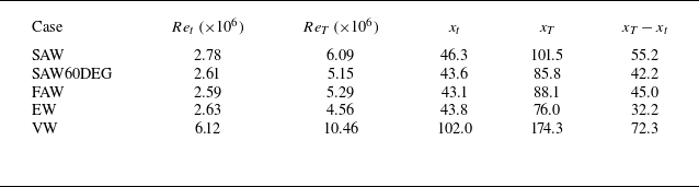


 Open access