





Non-technical Summary
Using computational simulation experiments, we investigated how distribution parameters affect the minimum sample size required to detect dimorphism in univariate variables. We constructed an artificial neural network model based on simulation results and validated our model with datasets from extant avian and reptilian species. Our study provides novel insights into understanding the detection of bimodal patterns in phenotype distribution, based on metrics from extant avian populations, such as average body mass, adult sex ratio, and within-population body-mass standard deviation. Also, we estimated a specific numerical threshold indicating the minimum sample size necessary for detecting bimodal patterns in fossils.
Introduction
Diverse phenotypes within natural populations, encompassing intraspecific variations such as sex, age, size, shape, behavior, or physiology (Darwin Reference Darwin1859, Reference Darwin1871; Dobzhansky Reference Dobzhansky1970; Bolnick et al. Reference Bolnick, Amarasekare, Araújo, Bürger, Levine, Novak, Rudolf, Schreiber, Urban and Vasseur2011; Richardson et al. Reference Richardson, Urban, Bolnick and Skelly2014; Moran et al. Reference Moran, Hartig and Bell2016), form the foundation for natural selection and are a central focus of evolutionary theory (Bolnick et al. Reference Bolnick, Amarasekare, Araújo, Bürger, Levine, Novak, Rudolf, Schreiber, Urban and Vasseur2011; Richardson et al. Reference Richardson, Urban, Bolnick and Skelly2014; Moran et al. Reference Moran, Hartig and Bell2016). These intraspecific trait variations consist of genetic variability and phenotypic plasticity for a given sex and age class (Pigliucci Reference Pigliucci2001; Violle et al. Reference Violle, Enquist, McGill, Jiang, Albert, Hulshof, Jung and Messier2012) and reflect microgeographic adaptation, divergent selection, and incipient speciation (Kingsolver and Pfennig Reference Kingsolver and Pfennig2007; Richardson et al. Reference Richardson, Urban, Bolnick and Skelly2014), driven by mechanisms such as local adaptation, parental conditions, and phenotypic plasticity (Violle et al. Reference Violle, Enquist, McGill, Jiang, Albert, Hulshof, Jung and Messier2012). Regardless of the underlying mechanisms, the resulting intraspecific phenotypic variation has profound ecological implications, shaping the dynamic interplay between ecology and evolution, often referred to as “eco-evolutionary dynamics” (Pelletier et al. Reference Pelletier, Garant and Hendry2009; Hendry Reference Hendry2017).
Understanding the role of intraspecific polymorphism can be crucial in the unraveling of the mechanisms of adaptation, speciation processes, and the intricate interactions between organisms and their environment. There are classic cases of polymorphism, such as plant height in Anthoxanthum odoratum (Antonovics and Bradshaw Reference Antonovics and Bradshaw1970; Antonovics Reference Antonovics2006), intensity of dark pigmentation in Drosophila americana (Wittkopp et al. Reference Wittkopp, Stewart, Arnold, Neidert, Haerum, Thompson, Akhras, Smith-Winberry and Shefner2009), body shape in Eurasian perch Perca fluviatilis (Svanbäck et al. Reference Svanbäck, Eklöv, Fransson and Holmgren2008), pharyngeal jaw shape and body shape in cichlid Herichthys minckleyi (Swanson et al. Reference Swanson, Gibb, Marks and Hendrickson2003), and bill size in African estrildid finch Pyrenestes ostrinus (Smith Reference Smith1987). Especially, Darwin’s finches, renowned for their diverse beak sizes and shapes, enable different populations and species to exploit different food resources across the Galápagos Islands (Lack Reference Lack1947; Grant Reference Grant1986). A medium ground finch (Geospiza fortis) population demonstrates a bimodal distribution in beak size as a critical dual-context trait (Grant Reference Grant1986; Podos Reference Podos2001; Huber et al. Reference Huber, León, Hendry, Bermingham and Podos2007; Grant and Grant Reference Grant and Grant2008). This trait reflects differences not only in beak shape but also in diet (Abbott et al. Reference Abbott, Abbott and Grant1977), bite force (Herrel et al. Reference Herrel, Podos, Huber and Hendry2005), and other ecological and reproductive factors, highlighting the role of beak size in both food processing (Grant and Grant Reference Grant and Grant1997) and species recognition (Huber et al. Reference Huber, León, Hendry, Bermingham and Podos2007). Within this population, beak size and shape underwent rapid evolution in response to fluctuating seed availability (Grant and Grant Reference Grant and Grant1995, Reference Grant and Grant2002), emphasizing the significance of polymorphism in adaptation and speciation processes and the interaction of organisms with their environment.
Nevertheless, exploring polymorphism in phenotypic distributions within the fossil record presents methodological and interpretative challenges. The fossil record, inherently fragmentary and incomplete, often yields datasets of limited sample size that are also subject to sampling biases, thereby constraining the reliability of polymorphism detection (Mallon Reference Mallon2017). This limitation is particularly problematic when attempting to distinguish between monomorphism and polymorphism in a single trait. A unimodal distribution of the trait may reflect true monomorphism, but it could also result from insufficient sample size or preservational biases (Mallon Reference Mallon2017; Motani Reference Motani2021). The absence of direct genetic and environmental contexts necessitates the use of inferential methods, such as comparative morphometrics and paleoenvironmental reconstructions, to assess the phenotypic diversity and evolutionary trajectories of extinct taxa (Hunt et al. Reference Hunt, Bell and Travis2008; Hopkins and Smith Reference Hopkins and Smith2015).
In this study, we focused on dimorphism instead of polymorphism in a single trait, which allows for a more streamlined analysis. To detect dimorphism in a single trait, we need to detect whether the distribution pattern of this single univariate trait is unimodal or bimodal. We aimed to estimate the optimal sample size required to detect bimodal patterns in phenotypic distribution of the single trait. To achieve this, we conducted computer simulation experiments to explore how distribution patterns influence the minimum sample size required to detect bimodal distributions. A previous study by Godfrey et al. (Reference Godfrey, Lyon and Sutherland1993) demonstrated that the mean difference and standard deviation determine the minimum sample size required for detecting bimodal distribution. Additionally, Motani (Reference Motani2021) qualitatively explained through computer simulations that the standard deviation ratio and the relative population size ratio significantly influence this minimum sample size. However, these studies were limited to two similar subgroups of simple normal distributions (Godfrey et al. Reference Godfrey, Lyon and Sutherland1993; Motani Reference Motani2021), which do not accurately reflect the complexities of biological populations that can exhibit substantial variations in parameters such as mean, standard deviation, and skewness. Herein, we expanded the scope by considering a wider range of parameter variations and included skewness in our computer simulations—an aspect that had not been previously addressed. Furthermore, we simultaneously varied multiple parameters and quantitatively studied how distribution parameters jointly influence the minimum sample size required for detecting bimodal distributions.
According to the simulation experiment results, a model was built to estimate the minimum sample size for detecting bimodality based on key distribution parameters. Then, we analyzed population data of modern avians and reptiles to assess whether the relationships between minimum sample size for detecting bimodality and distribution parameters were accurately identified. Our findings led us to conclude that specific distribution characteristics significantly influence the minimum sample size required to detect phenotypic dimorphism, which can serve as a reference for understanding phenotypic dimorphism in fossil avian taxa as well as in non-avian theropod dinosaurs.
Methods
Overview
Because the probability density distribution of character measurements can be highly variable, we assumed that each phenotypic group within a population emanates from a distinct probability distribution, characterized by a unique set of parameters: mean, standard deviation, skewness, and relative population size (Supplementary Fig. S1). Based on these parameters, we defined six metrics to characterize the distribution of two phenotypic groups within a population: the dimorphism index (DI), absolute magnitude of the standard deviation of both groups (Abs SD), standard deviation ratio (SD ratio), absolute magnitude of the skewness of both groups (Abs Skew), skewness difference (Skew Diff), and the relative population size ratio of the two phenotypic groups (Pop ratio).
This investigation primarily focused on examining how these six metrics influenced the minimum sample sizes required to detect bimodal phenotypes. We conducted sampling across a spectrum of sample sizes for each combination of two hypothetical distributions that represent two members of a dimorphic species population. To ensure the robustness and reliability of the data for each specified sample size, random sampling was repeated 500 times (Supplementary Fig. S2).
Workflow
In this study, we generated two distinct probability distributions (skew-normal distribution) (Azzalini Reference Azzalini and Azzalini2013) describing dimorphic phenotypic variation of one trait within a population. Random samples were generated from these distributions of populations for subsequent analyses.
In probability theory and statistics, the skew-normal distribution is a continuous probability distribution that derives from the normal distribution (Azzalini Reference Azzalini and Azzalini2013). Here, the standard normal probability density function is denoted as $ \unicode{x03C6} (x) $
:
$ \unicode{x03C6} (x) $
:
 $$ \unicode{x03C6} (x)=\frac{1}{\sqrt{2\unicode{x03C0}}}{e}^{-\frac{x^2}{2}}\;\left(-\infty <x<\infty \right) $$
where e, also called Euler’s number, is a mathematical constant (Rice Reference Rice2006b), and the cumulative distribution function is denoted as $ \unicode{x03D5} (x) $
:
$ \unicode{x03D5} (x) $
:
 $$ {\displaystyle \begin{array}{c}\unicode{x03D5} (x)={\int}_{-\infty}^x\unicode{x03C6} (t)dt=\frac{1}{2}\left[1+ erf\left(\frac{x}{\sqrt{2}}\right)\right]\;\left(-\infty <x<\infty \right)\end{array}} $$
where erf is the error function (Rice Reference Rice2006b). It is obtained by integrating the probability density function from negative infinity to x. Then the probability density function of the skew-normal distribution with parameter $ \unicode{x03B1} $
is denoted as
$ \unicode{x03B1} $
is denoted as $ \unicode{x03C6} \left(x;\unicode{x03B1} \right) $
(Azzalini Reference Azzalini and Azzalini2013):
$ \unicode{x03C6} \left(x;\unicode{x03B1} \right) $
(Azzalini Reference Azzalini and Azzalini2013):
 $$ {\displaystyle \begin{array}{c}\unicode{x03C6} \left(x;\unicode{x03B1} \right)=2\unicode{x03C6} (x)\unicode{x03D5} \left(\unicode{x03B1} x\right)\;\left(-\infty <x<\infty \right)\end{array}} $$
For applied work, location and scale parameters ( $ \xi $
and
$ \xi $
and $ \unicode{x03C9} $
) must be introduced (Azzalini Reference Azzalini and Azzalini2013):
$ \unicode{x03C9} $
) must be introduced (Azzalini Reference Azzalini and Azzalini2013):
 $$ {\displaystyle \begin{array}{c}Y=\unicode{x03BE} +\unicode{x03C9} x\end{array}} $$
Here, Y is a skew-normal variable. So that, the skew-normal probability density function with location $ \unicode{x03BE} $
, scale
$ \unicode{x03BE} $
, scale $ \unicode{x03C9} $
, and parameter
$ \unicode{x03C9} $
, and parameter $ \unicode{x03B1} $
becomes:
$ \unicode{x03B1} $
becomes:
 $$ {\displaystyle \begin{array}{c}f(Y)=\unicode{x03C6} \left(\frac{Y-\unicode{x03BE}}{\unicode{x03C9}};\unicode{x03B1} \right)=\frac{2}{\unicode{x03C9}}\unicode{x03C6} \left(\frac{Y-\unicode{x03BE}}{\unicode{x03C9}}\right)\unicode{x03D5} \left(\unicode{x03B1} \frac{Y-\unicode{x03BE}}{\unicode{x03C9}}\right)\left(-\infty <Y<\infty \right)\end{array}} $$
We can express the probability distribution using the skew-normal distribution:
 $$ {\displaystyle \begin{array}{c}Y\sim SN\left(\unicode{x03BE}; \hskip0.2em ;{\unicode{x03C9}}^2;\hskip0.2em ;\unicode{x03B1} \right)\end{array}} $$
where Y is a skew-normal (SN) variable with location parameter $ \unicode{x03BE} $
, scale parameter
$ \unicode{x03BE} $
, scale parameter $ \unicode{x03C9} $
, and slant parameter
$ \unicode{x03C9} $
, and slant parameter $ \unicode{x03B1} $
, and its density function is 5 (Azzalini Reference Azzalini and Azzalini2013). Then the probability distributions of the trait in two distinct phenotypic groups were hypothesized to follow skew-normal distributions, represented as:
$ \unicode{x03B1} $
, and its density function is 5 (Azzalini Reference Azzalini and Azzalini2013). Then the probability distributions of the trait in two distinct phenotypic groups were hypothesized to follow skew-normal distributions, represented as:
 $$ {\displaystyle \begin{array}{c}{Y}_1\sim SN\left({\unicode{x03BE}}_1;\hskip0.2em ;{\unicode{x03C9}_1}^2;\hskip0.2em ;{\unicode{x03B1}}_1\right)\end{array}} $$
 $$ {\displaystyle \begin{array}{c}{Y}_2\sim SN\left({\unicode{x03BE}}_2;\hskip0.2em ;{\unicode{x03C9}_2}^2;\hskip0.2em ;{\unicode{x03B1}}_2\right)\end{array}} $$
Here Y 1 and Y 2 are continuous random variables indicating one trait in two distinct phenotypic groups. These distributions are uniquely defined by three parameters derived from moments: first raw moment (mean), positive square root of second central moment (standard deviation), and normalized third central moment (skewness) (Rice Reference Rice2006a):
Mean:
 $$ {\displaystyle \begin{array}{c}\unicode{x03BC} =E\left\{Y\right\}=\unicode{x03BE} +\unicode{x03C9} {\unicode{x03BC}}_Z\;\left(Y\sim SN\right)\end{array}} $$
Standard deviation:
 $$ {\displaystyle \begin{array}{c}\unicode{x03C3} ={\left(E\left\{{\left(Y-E\left\{Y\right\}\right)}^2\right\}\right)}^{\frac{1}{2}}=\unicode{x03C9} {\unicode{x03C3}}_Z\;\left(Y\sim SN\right)\end{array}} $$
Skewness:
 $$ {\displaystyle \begin{array}{c}{\unicode{x03B3}}_1\left\{Y\right\}=\frac{E\left\{{\left(Y-E\left\{Y\right\}\right)}^3\right\}}{E{\left\{{\left(Y-E\left\{Y\right\}\right)}^2\right\}}^{\frac{3}{2}}}=\frac{4-\unicode{x03C0}}{2}\frac{\unicode{x03BC}_Z^3}{\unicode{x03C3}_Z^3}\;\left(Y\sim SN\right)\end{array}} $$
where
 $$ {\displaystyle \begin{array}{c}{\unicode{x03BC}}_Z=\sqrt{\frac{2}{\unicode{x03C0}}}\cdotp \unicode{x03B4}, {\unicode{x03C3}}_Z^2=1-{\unicode{x03BC}}_Z^2\end{array}} $$
The mean, or the expected value, is a measure of the location of a density or a frequency function (Rice Reference Rice2006a; Supplementary Fig. S3A). The standard deviation is a measure of dispersion about the mean (Rice Reference Rice2006a; Supplementary Fig. S3B). The skewness is a measure of the asymmetry of a density or a frequency function about its mean (Rice Reference Rice2006a; Supplementary Fig. S3C). Moreover, the population size of each group was also specified (Supplementary Fig. S3D).
Based on these parameters, we employed these six metrics to characterize the distributions within two distinct phenotypic groups: the DI, the Abs SD, the SD ratio, the Abs Skew, the Skew Diff, and the Pop ratio (Supplementary Fig. S4). The definitions for these six metrics are as follows:
 $$ {\displaystyle \begin{array}{c}\mathrm{DI}=\left(\mathrm{mean}\ \mathrm{of}\ \mathrm{population}\hskip0.3em 2/\mathrm{mean}\ \mathrm{of}\ \mathrm{population}\;1\right)-1\end{array}} $$
 $$ {\displaystyle \begin{array}{c}\mathrm{Abs}\hskip0.3em \mathrm{SD}=\\ {}\sqrt{\mathrm{standard}\ \mathrm{deviation}\ \mathrm{in}\ \mathrm{population}\hskip0.3em 1\hskip0.2em \ast \hskip0.3em \mathrm{standard}\ \mathrm{deviation}\ \mathrm{in}\ \mathrm{population}\hskip0.3em 2}\end{array}} $$
 $$ {\displaystyle \begin{array}{c}\mathrm{SD}\hskip0.2em \mathrm{ratio}=\\ {}\mathrm{standard}\ \mathrm{deviation}\ \mathrm{in}\ \mathrm{population}\hskip0.2em 2/\mathrm{standard}\ \mathrm{deviation}\ \mathrm{in}\ \mathrm{population}\hskip0.2em 1\end{array}} $$
 $$ {\displaystyle \begin{array}{c}\mathrm{Abs}\hskip0.2em \mathrm{Skew}=\\ {}\left(\mathrm{skewness}\ \mathrm{in}\ \mathrm{population}\hskip0.2em 2+\mathrm{skewness}\ \mathrm{in}\ \mathrm{population}\hskip0.2em 1\right)/2\end{array}} $$
 $$ {\displaystyle \begin{array}{c}\mathrm{Skew}\ \mathrm{Diff}=\\ {}\mathrm{skewness}\ \mathrm{in}\ \mathrm{population}\hskip0.2em 2-\mathrm{skewness}\ \mathrm{in}\ \mathrm{population}\hskip0.2em 1\end{array}} $$
 $$ {\displaystyle \begin{array}{c}\mathrm{Pop}\hskip0.2em \mathrm{ratio}=\\ {}\mathrm{population}\ \mathrm{size}\ \mathrm{of}\ \mathrm{population}\hskip0.2em 2/\mathrm{population}\ \mathrm{size}\ \mathrm{of}\ \mathrm{population}\hskip0.2em 1\end{array}} $$
Accordingly, four computational simulation experiments were designed to systematically investigate how the minimum sample size required for detecting bimodal phenotypes varies with changes in these metrics. Each simulation experiment focused on manipulating one parameter while keeping the others constant, thereby altering the distribution patterns. The following simulation experiments were conducted to explore: (1) the role of the DI in determining the minimum sample size; (2) the role of the Abs SD and the SD ratio in determining the minimum sample size; (3) the role of the Abs Skew and the Skew Diff in determining the minimum sample size; and (4) the role of the Pop ratio in determining the minimum sample size.
For each combination of two hypothetical distributions in an experiment, random sampling was performed with varying sample sizes, ranging from 10 to 1000. We selected the following 31 sample sizes as representative:
 $$ n=10,20,30,40,50,60,70,80,90,100, $$
 $$ 120,140,160,180,200,250,300,350,400,450, $$
 $$ 500,550,600,650,700,750,800,850,900,950,1000 $$
For each specific sample size (e.g., n = 100), 500 repeated samplings were performed. Then, for each replication, the generated data were subjected to an ACR test (Ameijeiras-Alonso, Crujeiras, Rodríguez-Casal test) to determine whether the bimodal distribution could be identified (Ameijeiras-Alonso et al. Reference Ameijeiras-Alonso, Crujeiras and Rodríguez-Casal2019). The ACR test combines excess mass and smoothing approaches to test for unimodal or bimodal distribution in univariate data with fewer errors than the dip test (Ameijeiras-Alonso et al. Reference Ameijeiras-Alonso, Crujeiras and Rodríguez-Casal2019). The number of replicates used in the test was set as 500, and the significance level employed for testing was set as 0.05. Consequently, each replication yielded a p-value. For the set of 500 p-values, the 95th percentile was calculated. If the 95th percentile was less than 0.05, it was determined that bimodal distribution can be detected at that particular sample size.
Then, based on the simulation results, we developed a prediction model for estimating the minimum sample size required to detect bimodality by training an artificial neural network (ANN). This approach not only enhances predictive accuracy but also contributes to advancing statistical methodologies in paleontology (Zhou Reference Zhou2021). We employed neural networks using resilient back-propagation with weight backtracking (Riedmiller Reference Riedmiller1994). Neural networks were trained with one hidden layer, consisting of 32 hidden neurons; the maximum steps for the training of the neural network were set as 1e + 08; the activation function was set as the logistic function; and the function used for the calculation of the error was set as the sum of the squared errors (Zhou Reference Zhou2021).
Finally, we used neontological data to test the model and estimate the minimum sample size for detecting bimodality. The datasets used were: beak length of the medium-sized finch species (Geospiza fortis) that display two phenotypes (Beausoleil et al. Reference Beausoleil, Carrión, Podos, Camacho, Rabadán-González, Richard and Lalla2023), body mass of the white-browed coucal bird (Centropus superciliosus) that displays sexual dimorphism (Goymann et al. Reference Goymann, Makomba, Urasa and Schwabl2015), and pelvic measurements of the American alligator (Alligator mississippiensis) that displays sexual dimorphism (Prieto-Marquez et al. Reference Prieto-Marquez, Gignac and Joshi2007).
Code and Dataset
All computational simulations experiments and analyses using the ANN model were performed in R (R Core Team Reference Team2024). To optimize computational efficiency, the simulation data generation and subsequent bimodal testing were executed on a high-performance computing blade server. Each experimental set utilized eight computing nodes, with each node employing 100 cores for parallel processing.
The code to generate simulation data, construct ANN models, and make predictions is available on GitHub. The simulation data produced by the program and neontological data used in this study are available on Dryad.
Results
Effect of the Dimorphism Index in Determining the Required Minimum Sample Size for Detecting Bimodality
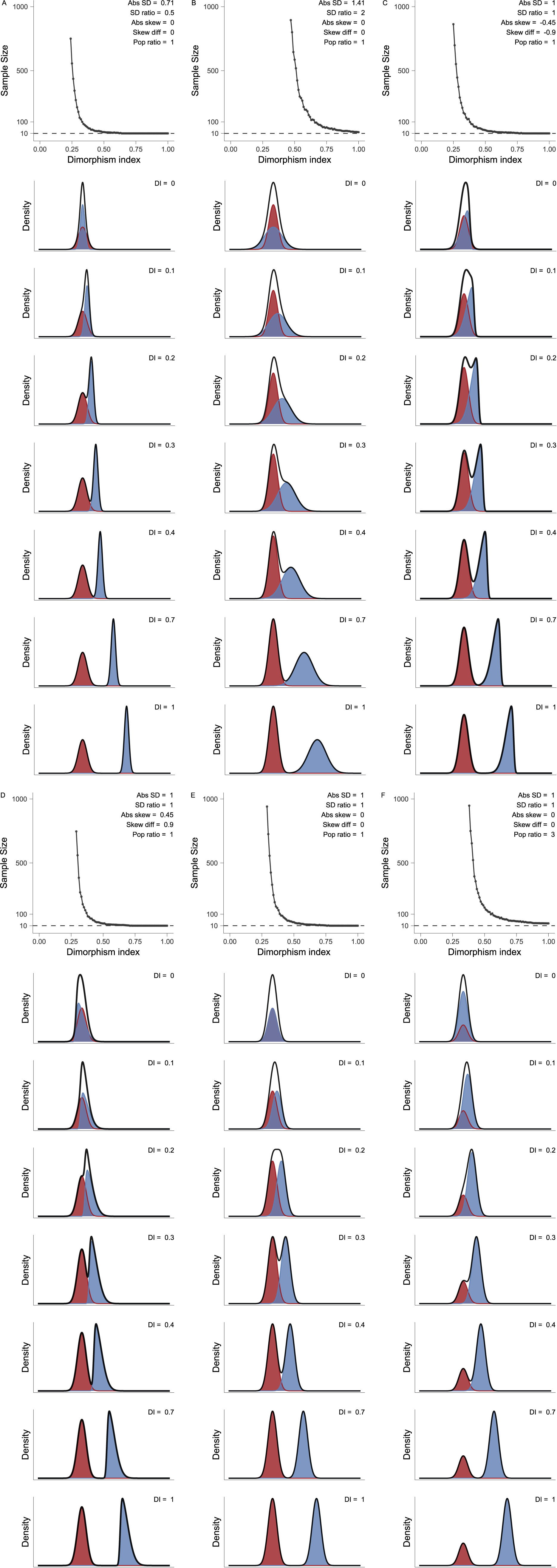
The results of these experiments focused on manipulating the DI to understand its relationship with sample size and ability to detect bimodal data distribution (assuming a skew-normal distribution model). The experiments were conducted with various settings, including different values for Abs SD, SD ratio, Abs Skew, Skew Diff, and Pop ratio. In the first experiment, we maintained Abs Skew at 0, Skew Diff at 0, Pop ratio at 1, and systematically adjusted Abs SD and SD ratio (Fig. 1A,B). In the initial scenario, setting Abs SD to $ \surd 0.5 $
and SD ratio to 0.5, it was observed that the requisite minimum sample size for identifying a bimodal distribution fell to 10 when the DI was greater than or equal to 0.64 (Fig. 1A). However, when the DI diminished to below 0.24, the minimum sample size for detecting bimodality drastically increased, surpassing 1000. The range between the DI values of 0.24 and 0.5 demonstrated an exponential reduction in the minimum sample size for detecting bimodality correlating with an increase in the DI, presenting a notable challenge in analyzing fossil data, as lower DI values necessitate substantially larger sample sizes for the reliable detection of bimodal distributions.
$ \surd 0.5 $
and SD ratio to 0.5, it was observed that the requisite minimum sample size for identifying a bimodal distribution fell to 10 when the DI was greater than or equal to 0.64 (Fig. 1A). However, when the DI diminished to below 0.24, the minimum sample size for detecting bimodality drastically increased, surpassing 1000. The range between the DI values of 0.24 and 0.5 demonstrated an exponential reduction in the minimum sample size for detecting bimodality correlating with an increase in the DI, presenting a notable challenge in analyzing fossil data, as lower DI values necessitate substantially larger sample sizes for the reliable detection of bimodal distributions.
Effect of the dimorphism index (DI) on sample size, illustrating the effect of the DI on minimum sample size when controlling other parameters. Each column represents a set of parameter combinations. For example, the first column (column A) represents the combination Abs SD = 0.71, SD ratio = 0.5, Abs skew = 0, Skew Diff = 0, and Pop ratio = 1. Line charts, the first image in each column, illustrate how the minimum sample size for detecting bimodality changes with variations in the DI. The subsequent images in each column, from top to bottom, demonstrate the changes in the distribution patterns of the two phenotypic subgroups as the DI increases. The red and blue probability plots represent the distribution patterns of the two phenotypic subgroups, while the black curve represents their combined distribution, that is, the overall population distribution. Abs SD, absolute standard deviation of both; SD ratio, standard deviation ratio; Abs Skew, absolute skewness of both; Skew Diff, skewness difference; Pop ratio, relative population size ratio.

A parallel trend was evident when the Abs SD and SD ratio were adjusted to $ \surd 2 $
and 2 (Fig. 1B). In this instance, the minimum sample size for detecting bimodality remained larger than 10 even when the DI reached 1. When the DI diminished below the threshold of 0.47, the minimum sample size escalated significantly, exceeding 1000. The interval between the DI values of 0.47 and 0.72 witnessed a similar exponential decrease in the minimum sample size with an increasing DI. These results suggested the relationship between the DI and the minimum sample size for detecting bimodality is consistent across varying SD, emphasizing the importance of considering DI values in fossil data analysis.
$ \surd 2 $
and 2 (Fig. 1B). In this instance, the minimum sample size for detecting bimodality remained larger than 10 even when the DI reached 1. When the DI diminished below the threshold of 0.47, the minimum sample size escalated significantly, exceeding 1000. The interval between the DI values of 0.47 and 0.72 witnessed a similar exponential decrease in the minimum sample size with an increasing DI. These results suggested the relationship between the DI and the minimum sample size for detecting bimodality is consistent across varying SD, emphasizing the importance of considering DI values in fossil data analysis.
Subsequently, the experimental framework was expanded to scenarios where the Abs SD was fixed at 1, SD ratio at 1, and Pop ratio at 1 (Fig. 1C,D). When Abs Skew and Skew Diff were set to −0.45 and −0.9 respectively, the results maintained consistent trends, revealing that a DI exceeding 0.79 yielded a minimum sample size of 10 for identification of bimodal distribution. Conversely, when the DI dropped below 0.25, the minimum sample size exceeded 1000. The range of DI values from 0.25 to 0.43 exhibited an exponential decrease in the minimum sample size as the DI increased. Additionally, when the Abs Skew and Skew Diff were set to 0.45 and 0.9, a DI greater than 0.71 resulted in a minimum sample size of 10 for the identification of bimodal distribution. In contrast, a DI falling 0.25 resulted in the minimum sample size exceeding 1000. Within the DI range spanning 0.25 to 0.52, a comparable exponential decrease in the minimum sample size for detecting bimodality was observed, in direct proportion to the increasing DI values. These findings collectively underscored a consistent relationship between the DI and the minimum sample size required for detecting bimodality across varied skewness compositions (comprising Abs Skew and Skew Diff), thus once again highlighting the importance of considering DI values in fossil data analysis.
Further investigation considered scenarios with the Abs SD at 1, SD ratio at 1, Abs Skew at 0, Skew Diff at 0, and the Pop ratio set to 1 and 3, respectively; the results revealed congruent trends (Fig. 1E,F). In scenarios where the Pop ratio was set to 1, a DI greater than or equal to 0.78 resulted in a minimum sample size of 10 for the identification of bimodal distribution, while a DI below 0.29 resulted in the minimum sample size exceeding 1000. The range between DI values of 0.29 and 0.52 exhibited an exponential decrease in the minimum sample size for detecting bimodality with an increasing DI.
In scenarios where the Pop ratio was set to 3, even a DI reaching 1 resulted in a minimum sample size larger than 10 for the identification of bimodal distribution, while a DI below 0.38 resulted in the minimum sample size exceeding 1000. In this case, the range of DI values from 0.38 to 0.62 exhibited an exponential decrease in the minimum sample size with an increasing DI. These findings suggested that the DI has a significant impact on the minimum sample size for detecting bimodality under varying conditions.
These simulations illustrated the significant role of the DI in determining the minimum sample size required for the accurate identification of bimodal distributions. As the DI increases, a discernible trend reveals a decreasing required minimum sample size for detecting bimodality, characterized by a nuanced transition from rapid to gradual reduction before ultimately converging to a minimum value (Fig. 1). Conversely, lower DI values presented significant challenges, requiring substantially larger sample sizes for the reliable identification of bimodal distributions. Such a trend remains consistent across various metrics sets of Abs SD, SD ratio, Abs Skew, Skew Diff, and Pop ratio, although differing subtly in the minimum DI required to identify bimodal distribution when the sample size is smaller than 1000.
Furthermore, DI can be expressed by a function of the mean difference (MD) and location of mode (LM) as follows:
 $$ {\displaystyle \begin{array}{c}\mathrm{DI}=\frac{2\mathrm{MD}}{2\mathrm{LM}-\mathrm{MD}}\end{array}} $$
The location parameter was proven to have no influence on the minimum sample size for detecting bimodality (Fig. 2), so when the DI influences the minimum sample size for detecting bimodality, it is the mean difference that influences the minimum sample size for detecting bimodality.
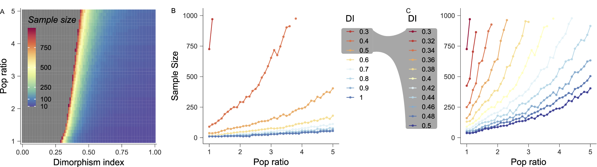
Effect of the absolute magnitude of mean (Abs mean), expressed as mean difference (MD) in main text, and the mean difference, expressed as location of mode (LM) in main text, on the minimum sample size for detecting bimodality. A, Heat map illustrating how the minimum sample size for detecting bimodality varies with the combined changes in the Abs mean and mean difference. Differences in colors indicate different minimum sample sizes for detecting bimodality. B, Line chart between the minimum sample size for detecting bimodality and the Abs mean. Each line shows how the minimum sample size for detecting bimodality changes with variations in the Abs mean at a constant mean difference, with different lines representing different mean differences. C, Line chart between the minimum sample size for detecting bimodality and mean difference. Each line shows how the minimum sample size for detecting bimodality changes with variations in the mean difference at a constant Abs mean, with different lines representing different Abs means.

Effect of the Dimorphism Index and Standard Deviation in Determining the Required Minimum Sample Size for Detecting Bimodality
With the DI as the pivotal factor, we next examined the impact of the standard deviation on the essential minimum sample size for detecting bimodal distributions. The standard deviation encompasses three critical dimensions: Abs SD, SD ratio, and the standard deviation specific to one of the groups.
The initial segment of this analysis centered on the role played by the absolute magnitude of the standard deviation within both groups (Figs. 3, 4). This examination was conducted under a controlled paradigm where the SD ratio was held constant, with the Abs Skew set at 0, Skew Diff set at 0, and Pop ratio set at 1. This allowed for an isolated study of variations in both the DI and the absolute magnitude of the standard deviation concerning the required minimum sample size for detecting bimodality. Moreover, three parallel experimental designs were executed to qualitatively study the effect of the SD ratio. Within these distinct experimental configurations, the SD ratio was varied, with the assigned values being 1, 1.25, and 1.5, respectively (Fig. 5).
Distribution patterns with changes in dimorphism index (DI) and absolute magnitude of the standard deviation of both groups (Abs SD) at a constant standard deviation ratio (SD ratio). The horizontal arrow represents changes in the DI, while the vertical arrows represent changes in the Abs SD.

Distribution patterns with changes in dimorphism index (DI) and absolute magnitude of the standard deviation of both groups (Abs SD) on the left and the corresponding ACR test results on the right. The left column displays the distribution patterns, corresponding to the nine plots in Fig. 3. In each row, the plot on the right shows the results of the ACR test for simulation data, which was generated from the distribution pattern on the left. For each distribution pattern combination, random sampling was performed with varying sample sizes, ranging from 10 to 1000. For each specific sample size (e.g., n = 100), 500 repeated samplings were performed.

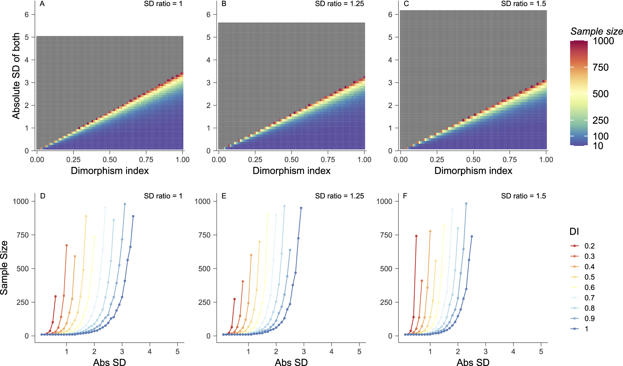
Effect of the dimorphism index (DI) and absolute magnitude of the standard deviation of both groups (Abs SD) on the minimum sample size for detecting bimodality. A–C, Heat maps illustrating how the minimum sample size varies with the combined changes in the DI and Abs SD. Differences in color indicate different minimum sample sizes for detecting bimodality. The gray area indicates that the minimum sample size for detecting bimodality exceeds 1000. D–F, Line charts showing the relationship between sample size and Abs SD. Each line shows how the minimum sample size for detecting bimodality changes with variations in the Abs SD at a constant DI, with different lines representing different DIs. A–D, B–E, and C–F represent three parallel experiments with different standard deviation ratios (SD ratio): 1, 1.25, and 1.5, respectively.

When the SD ratio was set at 1, the results revealed a positive correlation between the Abs SD and the minimum sample size required to recognize bimodal signals (Figs. 4, 5A,D). These findings demonstrated a direct correlation between an increase in the absolute magnitude of the standard deviation and a concurrent increase in the required minimum sample size for detecting bimodality. These trends persisted across varying SD ratio (1, 1.25, 1.5), highlighting consistent patterns of change in response to alterations in both the absolute magnitude of the standard deviation and the DI.
Furthermore, when the SD ratio increases from 1 to 1.25, maintaining the same Abs SD and DI, the minimum sample size required for detecting bimodality increases (Fig. 5B,E). When the SD ratio increased to 1.5, the required minimum sample size also exhibited an increase (Fig. 5C,F).
When the Abs SD was set at 1, the results revealed a positive correlation between the SD ratio and the minimum sample size required to recognize bimodal signals (Fig. 6). The findings demonstrated a direct correlation between an increase in the SD ratio and a concurrent increase in the required minimum sample size for detecting bimodality. Conversely, a larger DI was associated with a reduction in the required minimum sample size for detecting bimodality. These trends persisted across varying Abs SD (1, 1.5, 2) (Fig. 6), highlighting consistent patterns of change in response to alterations in both the absolute magnitude of the standard deviation and the DI.
Effect of the dimorphism index (DI) and standard deviation ratio (SD ratio) on the minimum sample size. A–C, Heat maps illustrating how the minimum sample size varies with the combined changes in DI and SD ratio. Differences in color indicate different sample size. The gray area indicates that the minimum sample size for detecting bimodality exceeds 1000. D–F, Line charts showing the relationship between sample size and SD ratio. Each line shows how the minimum sample size for detecting bimodality changes with variations in the SD ratio at a constant DI, with different lines representing different DIs. A–D, B–E, and C–F represent three parallel experiments with Abs SD: 1, 1.5, and 2, respectively.

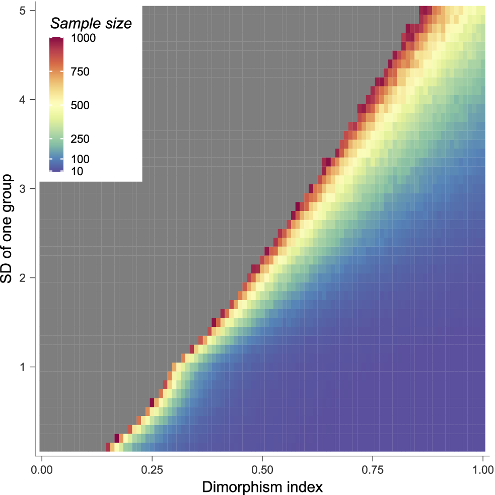
In scenarios where the standard deviation of one group was held constant while that of the other was varied (Supplementary Fig. S5), the results consistently indicated that a larger standard deviation necessitates a correspondingly larger required minimum sample size for the identification of bimodal distribution (Supplementary Figs. S6, S7). Differing from the linear relationships between the minimum sample size for detecting bimodality and the absolute magnitude of standard deviation, relationships between the minimum sample size for detecting bimodality and the standard deviation of one group displayed nonlinear relationships (Fig. 7), thus further explaining the effect of the SD ratio.
Heat map illustrating how the minimum sample size for detecting bimodality varies with the combined changes in the dimorphism index (DI) and standard deviation of one group (SD of one group). Differences in color indicate different minimum sample sizes for detecting bimodality. The gray area indicates that the minimum sample size for detecting bimodality exceeds 1000.

Effect of the Dimorphism Index and Skewness in Determining the Required Minimum Sample Size for Detecting Bimodality
In the subsequent phase of the study, we investigated the influence of skewness on the minimum sample size required for detecting bimodal distribution. Skewness encompasses three essential dimensions: Abs Skew, Skew Diff, and the specific skewness value associated within one group.
This investigation was initiated by assessing the impact of the absolute magnitude of skewness within the two groups. In this context, with the Abs SD at 0, SD ratio at 1, Pop ratio at 1, and keeping the Skew Diff constant, we exclusively manipulated the Abs Skew and the DI, thereby evaluating their collective influence on the required minimum sample size for detecting bimodality (Supplementary Figs. S7, S8). This facet of the study involved the implementation of three parallel experimental groups, each characterized by distinct Skew Diffs, assigned values of 0, 0.25, and 0.5 respectively (Fig. 8), to examine how Skew Diff influences the minimum sample size required to identify bimodal patterns.
Effect of the dimorphism index (DI) and absolute magnitude of the skewness of both groups (Abs Skew) on the minimum sample size for detecting bimodality. A–C, Heat maps illustrating how the minimum sample size varies with the combined changes in DI and Abs Skew. Differences in color indicate different sample sizes. The gray area indicates that the minimum sample size for detecting bimodality exceeds 1000. D–I, Line charts showing the relationship between sample size and Abs Skew. Each line shows how the minimum sample size changes with variations in the Abs Skew at a constant DI, with different lines representing different DIs. A–D–G, B–E–H, and C–F–I represent three parallel experiments with skewness difference (Skew Diff): 0, 0.25, and 0.5, respectively. When the DI ranges from 0.3 to 0.4, the relationship between the sample size and Abs Skew is more significantly influenced by the DI. Therefore, G–H–I further illustrates the changes in sample size with variations in the Abs Skew for DI values between 0.3 and 0.4, providing additional information to supplement D–E–F.

When the Skew Diff was set at 0, the results demonstrated that when the DI value remains unchanged, deviations of the Abs Skew from 0, whether positive or negative, were associated with a reduction in the minimum sample size required to identify the bimodal pattern (Figs. 8A,D,G, Supplementary Fig. S8). Nevertheless, it was observed that the impact of the Abs Skew appeared to be relatively limited. Notably, when the DI reached a sufficiently high threshold, such as 0.5 or above, the requisite minimum sample size for the detection of bimodal distributions became markedly reduced, irrespective of variations in the Abs Skew (Fig. 8A–C). Furthermore, these trends persisted across varied Skew Diff (0, 0.25, 0.5), highlighting persistent patterns of change in response to alterations in both the absolute magnitude skewness and the DI.
Limited changes in patterns were observed among varying Skew Diff values, indicating that the relative impact of Skew Diff on the required minimum sample size for detecting bimodality was comparatively modest (Fig. 9). Notably, a pronounced influence of the Skew Diff was observed, particularly when the DI was less than around 0.34 (Fig. 9G,H,L). When the Abs Skew and DI were held constant, the sample size necessary to detect bimodality initially increased and then decreased as the Skew Diff increased (Fig. 9). This indicates that as the Skew Diff increases, the depth of the gap between the two peaks first decreases and then increases. Additionally, the position of the turning point or maximum value shifts with changes in the DI. For example, with Abs Skew = 0 and DI = 0.3, as the Skew Diff increased from −1.9 to approximately 0.8, the required minimum sample size for detecting bimodality gradually increased (Fig. 9K), while as the Skew Diff continued to increase from around 0.8 to 1.9, the required minimum sample size for detecting bimodality rapidly decreased (Fig. 9K).
Effect of the dimorphism index (DI) and skewness difference (Skew Diff) on the minimum sample size for detecting bimodality. A–C and J, Heat maps illustrating how the minimum sample size for detecting bimodality varies with the combined changes in the DI and Skew Diff. Differences in color indicate different minimum sample sizes for detecting bimodality. The gray area indicates that the minimum sample size for detecting bimodality exceeds 1000. D–I, K, and L, Line charts showing the relationship between the sample size and Skew Diff. Each line shows how the minimum sample size for detecting bimodality changes with variations in the Skew Diff at a constant DI, with different lines representing different DIs. A–D–G, B–E–H–J–K–L, and C–F–I represent three parallel experiments with Abs Skew: −0.5, 0, and 0.5, respectively. When the DI ranges from 0.3 to 0.4, the relationship between the sample size and Skew Diff is more significantly influenced by the DI. Therefore, G–H–I and L further illustrate the changes in sample size with variations in Skew Diff for DI values between 0.3 and 0.4, providing additional information to supplement D–E–F and K. When Abs Skew = 0, the Skew Diff exhibits a wider range of variation (−1.9 to 1.9). Therefore, J, K, and L specifically show how the minimum sample size for detecting bimodality changes as the Skew Diff ranges from −1.9 to 1.9. To allow for parallel comparison with Abs Skew = −0.5 (A–D–G) and 0.5 (C–F–I), B–E–H are retained, where the Skew Diff ranges from −0.9 to 0.9, consistent with A–D–G and C–F–I.

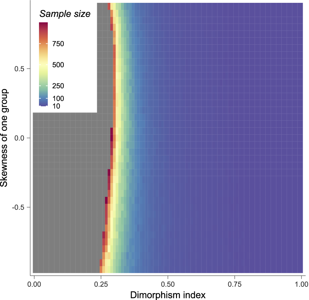
Moreover, in scenarios where skewness was kept constant for one group while being varied in another group (Supplementary Figs. S9, S10), the results consistently indicated that the greater the deviation of skewness from 0, the lesser the minimum sample size for detecting bimodality (Fig. 10, Supplementary Fig. S10). Contrary to symmetrical patterns of the relationship between the minimum sample size for detecting bimodality and absolute magnitude skewness (Fig. 8), the impact of specific skewness value associated within one group on minimum sample size for detecting bimodality was asymmetric (Fig. 10), demonstrating that Skew Diff does influence, although weakly, the minimum sample size for detecting bimodality.
Heat map illustrating how the minimum sample size for detecting bimodality varies with the combined changes in the dimorphism index (DI) and skewness of one group. Differences in color indicate different minimum sample sizes for detecting bimodality. The gray area indicates that the minimum sample size for detecting bimodality exceeds 1000.

Effect of the Dimorphism Index and Relative Population Size Ratio in Determining the Required Minimum Sample Size for Detecting Bimodality
With the DI as the pivotal factor, we finally examined the effects of Pop ratio on the essential minimum sample size required for detecting bimodal distribution (Supplementary Fig. S11). We manipulated the DI and Pop ratio as variable metrics, while maintaining constancy in the standard deviation and skewness values (the Abs SD at 1, SD ratio at 1, Abs Skew at 0, and Skew Diff at 0) (Fig. 11, Supplementary Fig. S12).
Effect of the dimorphism index (DI) and relative population size ratio of the two phenotypic groups (Pop ratio) on the minimum sample size for detecting bimodality. A, Heat map illustrating how the minimum sample size for detecting bimodality varies with the combined changes in the DI and Pop ratio. Differences in colors indicate different sample size. The gray area indicates that the minimum sample size for detecting bimodality exceeds 1000. B and C, Line charts showing the relationship between the minimum sample size for detecting bimodality and Pop ratio. Each line shows how minimum sample size for detecting bimodality changes with variations in Pop ratio at a constant DI, with different lines representing different DIs. When the DI ranges from 0.3 to 0.5, the relationship between the minimum sample size for detecting bimodality and Pop ratio is more significantly influenced by the DI. Therefore, C further illustrates the changes in the minimum sample size for detecting bimodality with variations in the Pop ratio for the DI values between 0.3 and 0.5, providing additional information to supplement B.

Results revealed that an increase in the Pop ratio necessitates an increase in the minimum sample size required for the effective detection of a bimodal distribution under a constant DI (Fig. 11A). This trend was observed across different DI values. Notably, when the DI value fell within the range of 0.3 to 0.5, the impact of the Pop ratio became particularly noteworthy (Fig. 11C). However, when the DI value was sufficiently large, such as 0.7 or larger, change of the Pop ratio value had almost no discernible effect on the minimum sample size required for identification of bimodal patterns (Fig. 11B). Conversely, elevation in the DI was found to be associated with a reduction in the minimum sample size for the effective detection of a bimodal distribution (Fig. 11A).
Mode Construction and Validation
Our simulations show that the mean difference, standard deviation, skewness, and population size ratio all significantly affect the minimum sample size. Higher-order moments are typically considered as more detailed descriptions of the shape of a distribution (Stuart and Ord Reference Stuart and Ord2010) and are thus viewed as less critical for characterizing a distribution compared with lower-order moments like mean and variance (Stuart and Ord Reference Stuart and Ord2010). However, skewness, albeit derived from a higher-order moment (Rice Reference Rice2006a), exhibits significant influence on determining the minimum sample size required for identifying bimodal distributions.
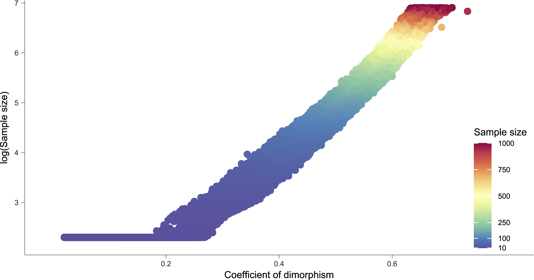
Based on the simulation data, we fit the minimum sample size for detecting bimodality to the regression function with respect to the coefficient of dimorphism (CD), which is defined as (SD1 + SD2)/mean difference, as well as the Abs SD, SD ratio, and Pop ratio. When the minimum sample size for detecting bimodality exceeds 10, the logarithm of the minimum sample size shows a strong linear relationship with the coefficient of dimorphism (Fig. 12). In this way, when obtaining the parameters (coefficient of dimorphism, Abs SD, SD ratio, and Pop ratio) of a certain trait of a biological population, the minimum sample size required to identify the bimodal distribution of that trait can be estimated.
 $$ {\displaystyle \begin{array}{c}\mathrm{Minimum}\ \mathrm{sample}\ \mathrm{size}=f\left(\mathrm{CD},\mathrm{Abs}\hskip0.32em \mathrm{SD},\mathrm{SD}\hskip0.32em \mathrm{ratio},\mathrm{Pop}\hskip0.42em \mathrm{ratio}\right)\end{array}} $$
Scatter plot of the minimum sample size for detecting bimodality and the coefficient of dimorphism, indicating the effect of the coefficient of dimorphism on the minimum sample size for detecting bimodality. Differences in color indicate different minimum sample sizes for detecting bimodality.

Here we employed ANN models to approximate the functional relationship between the minimum sample size and the input parameters. An exhaustive comparison of various parameter configurations was undertaken to identify the model configuration yielding the optimal predictive performance (Supplementary Fig. S13). This comparative analysis is crucial for elucidating the neural network architecture most adept at encapsulating the complex nonlinear relationships inherent to the minimum sample size estimation for identifying bimodal distributions in biological traits.
The medium-sized finch species (Geospiza fortis) displays two phenotypes of beak length (Beausoleil et al. Reference Beausoleil, Carrión, Podos, Camacho, Rabadán-González, Richard and Lalla2023), so their data are valuable for our model testing when considered without the prior identification of the two subgroups. We treated the true distribution of single-year data of this Darwin’s finches’ beak length as a population feature and calculated the four key metrics (CD, Abs SD, SD ratio, and Pop ratio) based on the prior identification of the two subgroups. Using these population metrics, we calculated the minimum sample size for detecting bimodal distribution with the model. If the population displays a unimodal distribution according to the mode test on the collected data, the minimum sample size for detecting bimodal distributions calculated by the model would be larger than the true sample size. Results indicated that all computed minimum sample sizes for detecting bimodality surpassed the actual sample sizes (Supplementary Table S1). Our results do not imply criticism of Beausoleil et al.’ s work, as their analysis relied on prior knowledge of the two subgroups identification.
Additionally, the white-browed coucal bird (Centropus superciliosus) displays sexual dimorphism in body mass (Goymann et al. Reference Goymann, Makomba, Urasa and Schwabl2015), and the American alligator (Alligator mississippiensis) displays sexual dimorphism in pelvic measurements (Prieto-Marquez et al. Reference Prieto-Marquez, Gignac and Joshi2007). These studies also provide valuable data for our model testing when considered without prior knowledge of sexual identification. The results of the ACR test on these two species demonstrated that such distributions are unimodal. We also used their population data to test the model we constructed. The outcomes presented earlier were congruent with the initial hypotheses that the computed minimum sample sizes for detecting bimodality surpass the actual sample sizes (Supplementary Table S1). Through this rigorous evaluation, the model remained unrefuted at the current juncture. Again, our results do not imply criticism of these previous works, as their analysis relied on prior knowledge of sexual identification.
Applications and Limitations
A Standard Minimum Sample Size for Detecting Bimodality in Fossil Populations
Given the evidence for sexual dimorphism in crocodilians (Webb and Messel Reference Webb and Messel1978; Prieto-Marquez et al. Reference Prieto-Marquez, Gignac and Joshi2007; Platt et al. Reference Platt, Rainwater, Thorbjarnarson, Finger, Anderson and McMurry2009) and birds (Darwin Reference Darwin1871; Goymann et al. Reference Goymann, Makomba, Urasa and Schwabl2015; Schoenjahn et al. Reference Schoenjahn, Pavey and Walter2020; Caron and Pie Reference Caron and Pie2024), the closest extant relatives of dinosaurs (Bryant and Russell Reference Bryant and Russell1992; Witmer Reference Witmer and Thomason1995), we suppose that sexual dimorphism, whether strong or weak, was present in at least some dinosaur taxa. However, to date, reliable evidence of sexual dimorphism in Mesozoic Avialae based on statistically robust analysis has only been found in Confuciusornis sanctus (Zhou et al. Reference Zhou, Pan, Wang, Wang, Zheng and Zhou2024). The reasons for this situation could be the limit of fossil specimens, weak signals of sexual dimorphism, or the actual absence of sexual dimorphism within these species. Therefore, a standardized way of determining whether the sample size is sufficient or not is crucial.
Until now, only ambiguous statements have been available as references, such as “strongly expressed dimorphism could be detected” (Motani Reference Motani2021) or “weakly expressed dimorphism could be impossible to detect” (Kościński and Pietraszewski Reference Kościński and Pietraszewski2004). Such statements provide low informational content and cannot serve as clear references. Providing a specific numerical threshold indicating the sample size, whether sufficient or insufficient, is much more effective and informative.
It is obvious that more is usually better in terms of sample size, and such a challenge typically resolves around the availability of that sample (Plavcan Reference Plavcan1994; Kościński and Pietraszewski Reference Kościński and Pietraszewski2004; Mallon Reference Mallon2017). However, our results place a potential constraint on sample size for statistically significant studies. Our study suggests that the minimum sample size required for detecting bimodal patterns is strongly dependent on the parameters of the density distribution of the measured character. Through a series of computer simulation experiments with multiple varying distribution parameters, we have estimated potential thresholds for different parameters of the distribution of univariate morphological variables. Thus, we built a model to estimate the minimum sample size for detecting bimodality based on simulation experiment results (Fig. 13), and this estimate can serve as a reference point. However, its utility is limited, as real biological populations are often structured in more complicated ways.
Schematic showing the simulation experiments, construction of the model, and the use of neontological data to test the model to estimate the minimum sample size for detecting bimodality. A–D, Steps of computer simulation experiment and model construction. E–G, Steps of estimating parameters of extant avian. H and I, Steps of model validation and estimate of the minimum sample size for detecting bimodality. A, A set of distribution patterns based on designed parameters. B, Relationship between the minimum sample size for detecting bimodality and the distribution parameters. C, Several sets of the relationship between the minimum sample size for detecting bimodality and the distribution parameters. D, Artificial neural network (ANN) model used to estimate the minimum sample size for detecting bimodality based on input distribution parameters: coefficient of dimorphism (CD), absolute magnitude of the standard deviation of both groups (Abs SD), standard deviation ratio (SD ratio), and relative population size ratio of the two phenotypic groups (Pop ratio). Specifically, the ANN includes one input layer with four input nodes (I1, I2, I3, and I4), one output layer with one output variable (O1), and one hidden layer with 32 nodes labeled as H1 through H32. Bias nodes (B1 and B2) are also connected to the hidden and output layer. Positive weights are plotted as black lines, and negative weights are plotted as gray lines between layers. Line thickness is in proportion to the relative magnitude of each weight. E, Plot of log(SD of body mass) versus log(mean of body mass) for estimating SD of body mass. F, Distribution of coefficient of dimorphism. G, Distribution of Pop ratio. H, Model validation according to neontological population data. I, Estimate of minimum sample size for detecting bimodality based on extant avian population data. All silhouettes were sourced PhyloPic (http://phylopic.org/) under a public domain license.

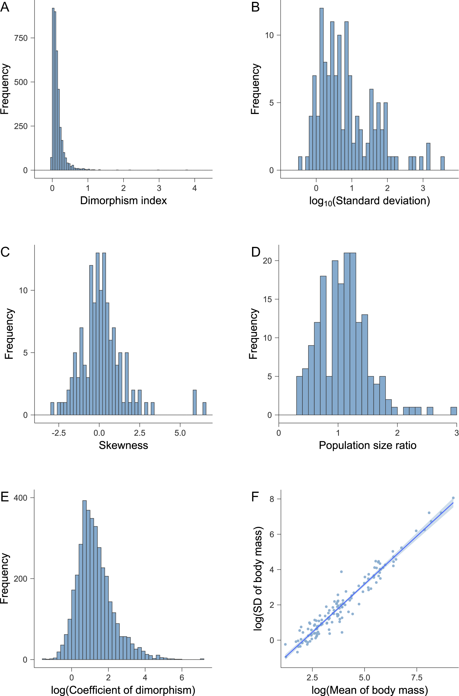
Considering that we could hardly calculate the distribution parameters of different sexes in fossil species without prior sexual determination, approximately estimating the probability of detecting sexual dimorphism is important. To determine whether fossil avian and non-avian theropod dinosaurs exhibit a single trait with a bimodal distribution caused by sexual dimorphism, we estimated the minimum sample size required for identifying bimodal distributions using population parameters from extant birds (Figs. 13E,F,G, 14). The accurate Mean difference was calculated based on the body mass of female and male extant birds using a published dataset (Gonzalez-Voyer et al. Reference Gonzalez-Voyer, Thomas, Liker, Krüger, Komdeur and Székely2022), which includes 3813 species, of which 98.11% exhibit sexual dimorphism in body mass (Fig. 14A). Due to the lack of a large database for the standard deviation (SD), its values were estimated through the regression relationship between the standard deviation and the mean (Fig. 13E), based on a database containing population data (Read et al. Reference Read, Baiser, Grady, Zarnetske, Record and Belmaker2018). In addition, the Pop ratio was estimated from the median of the adult sex ratio from Gonzalez-Voyer et al.’s dataset (2022).
Distribution of parameters from extant avian. A, Distribution of dimorphism index. B, Distribution of standard deviation. C, Distribution of standard skewness. D, Distribution of relative population size ratio. E, Distribution of coefficient of dimorphism. F, Scatter plots and regression line of log (SD of body mass) vs. log (mean of body mass). SD, standard deviation.

The results indicated that, when the sample size reaches 10 samples, 13.65% of birds can be identified with a bimodal distribution; at 100 samples, 19.21% can be identified; at 200 samples, 20.39% can be identified; at 500 samples, 22.13% can be identified; at 1000 samples, 23.15% can be identified; at 2000 samples, 24.07% can be identified; and at 5000 samples, 25.05% can be identified (Fig. 13I). Assuming the parameters of fossil avian species are included within those of extant birds, with a sample size of 200, it is possible to identify phenotypic dimorphism caused by sexual dimorphism in one-fifth of the species. Furthermore, samples sizes of more than 200 only minimally contributed to sexual dimorphism detection, because an increase of 25 times in sample size from 200 to 5000 only resulted in a 5% increase in the number of bird species identified with sexual dimorphism. So, 200 samples could be an important threshold value when we want to detect sexual dimorphism in fossil avian species.
Limitations
Our findings about standard minimum sample size significantly contribute to the refinement of methodologies in paleontological research by guiding researchers in optimizing sample sizes based on the characteristics of the data under investigation. However, these results are to some extent artificial, as the distribution was simulated to be normal or skew-normal and thus may not fully reflect the actual distribution of biological traits. Our primary focus was to understand how sample size influences the dynamics of dimorphisms without prior knowledge of the subgroups. The dynamics of dimorphisms in nature are more complex than our model suggests. It is essential to recognize that bimodality in univariate distributions does not necessarily indicate the presence of dimorphism (Schilling et al. Reference Schilling, Watkins and Watkins2002).
Our model simplified this relationship. For example, even when dimorphism exists, the combined population distribution may not exhibit bimodality due to overlapping distributions (Schilling et al. Reference Schilling, Watkins and Watkins2002). In our simulations, even with extremely large sample sizes, identifying bimodality in such scenarios remains elusive. This situation often requires prior knowledge of the sex or subgroups to accurately interpret the results (Saitta et al. Reference Saitta, Stockdale, Longrich, Bonhomme, Benton, Cuthill and Makovicky2020). Various methods for assessing sexual dimorphism (Plavcan Reference Plavcan1994; Rehg and Leigh Reference Rehg and Leigh1999) provide additional frameworks for understanding dimorphism beyond just bimodality.
Additionally, when estimating the minimum sample size required for fossil avialans using extant avian data, limitations in the available data prevented precise estimates for the SD ratio, Pop ratio, and skewness. In our model, we approximated the SD ratio as 1, the Pop ratio as the median of the extant avian dataset, and the skewness as 0, which may introduce some bias into the final estimates. Furthermore, the minimum sample size thresholds we identified can appear arbitrary and are influenced by various parameter values. Our analysis suggests that the threshold is approximately 200 and that increasing sample sizes beyond this point does not significantly enhance the ability to identify bimodality. It is important to emphasize that this threshold serves primarily as a reference point for fossil avialans.
Acknowledgments
We are grateful to C. R. Marshall for his valuable discussions regarding this paper. We would like to thank W. Song, K. Cao, and B. Zhang for their advice on the method, and Y. O’Connor for her assistance with English language/grammar. We thank the editor, M. Hopkins, associate editor, A. Dunhill, reviewers E. T. Saitta and P. Godoy, and an anonymous reviewer for their constructive comments that improved this article. This research was supported by the National Natural Science Foundation of China (42288201, 41922011), and the Fundamental Research Funds for the Central Universities No. 0206-14380219.
Competing Interests
The authors declare no competing interests.
Data Availability Statement
All code used in the article presented here are available from GitHub Repository: https://github.com/BOBOXY/Min-Sample-Size-Phenotypic-Dimorphism. All data used in the article are available from Dryad Digital Repository: https://doi.org/10.5061/dryad.08kprr5f9.







 Open access

