2. Mathematical formulation

A traditional Hele-Shaw cell consists of two parallel plates separated by a small distance, $b$, and filled with viscous fluid with viscosity, $\mu$. For the case of a circular geometry, like that depicted in figure 2, an inviscid fluid is injected at a point, and this drives an outwards-expanding interface between viscous and inviscid fluids.

We now consider the related wedge-shaped geometry, as shown in figure 3(a). Here, the inviscid fluid is injected at the wedge corner at some prescribed flow rate. The viscous fluid is constrained to lie between the wedge walls separated by an internal angle $\theta _0$. As can be observed experimentally (Thomé et al. 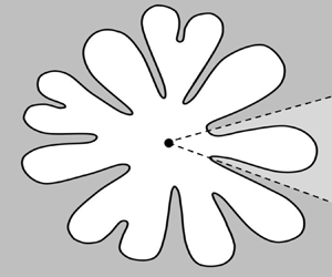Reference Thomé, Rabaud, Hakim and Couder1989), a self-similar shape is reached eventually, where the inviscid fluid occupies an angle $\lambda \theta _0$, with $0<\lambda <1$. This set-up is referred to as divergent flow in Ben Amar (Reference Ben Amar1991a). For the case of zero-surface-tension, a prototypical solution is shown in figure 3(a), and we observe the petal-shaped interface between viscous fluid and inviscid fluid.

Figure 3.

(a) A numerical plot of the top-down view of the self-similar physical profile in the $\hat {z}$-plane is shown for the zero-surface-tension case, with parameter values $\theta _0 = 20^{\circ }$ and $\lambda = 0.6$. The free surface was computed using (3.7). The Hele-Shaw cell is bounded by the thick black lines and is filled with a viscous fluid, shown in grey. An inviscid fluid is injected from the corner of the wedge and forms a finger with angle $\lambda \theta _0$. The corner of the wedge lies at $\hat z = 0$ ($BF$) and the tip of the finger lies at $\hat {z}=1$ ($CE$). (b) A sketch of the $z$-plane, computed via the conformal map $z=(2/\theta _0)\log \hat {z}$. This configuration is analogous to the traditional Saffman–Taylor finger (McLean & Saffman Reference McLean and Saffman1981).

The classic problem of Saffman–Taylor viscous fingering in a channel is typically studied in a travelling frame corresponding to a steady-state finger. In the wedge geometry, the analogue of a travelling wave frame of reference is a self-similar solution. In Appendix A, we demonstrate how the original equations of potential flow for a Hele-Shaw cell, with boundary conditions on the channel walls and free boundary, and an injection condition can be reposed in the self-similar framework. The key idea relates to a transformation of the original dimensional lengths, $\bar {x}$ and $\bar {y}$, which are scaled via

(2.1)\begin{equation} (\hat{x}, \hat{y}) = \frac{(\bar{x}, \bar{y})}{R_0 {A}(t)}, \end{equation}

where $R_0$ is a length scale (chosen to be the distance between the corner of the wedge and the tip of the finger at $t=0$) and ${A}(t)$ is a dimensionless scaling factor that depends on dimensionless time, $t$. As shown in Appendix A, two possible choices of ${A}(t)$ result in effectively the same self-similar problem, given by (A6), in dimensionless variables with a time-independent effective surface-tension parameter $\sigma$. This $\sigma$, when rescaled, then gives us our small parameter $\epsilon$, defined below in (2.10); see Ben Amar (Reference Ben Amar1991b) for further details.

We thus have the governing set of potential-flow equations in (A6) corresponding to a scaled velocity potential, $\hat {\phi }$, and self-similar physical-plane coordinates, written in complex form as $\hat {z} = \hat {x} + \mathrm {i} \hat {y}$ (figure 3a). Note that the free surface is now stationary. We introduce the complex potential, $\hat {f}=\hat {\phi }+\mathrm {i}\hat {\psi }$, with harmonic conjugate given by the streamfunction $\hat{\psi}$. Within the $\hat {f}$-plane, fluid is located in the infinite strip bounded by $\hat {\psi } \in [-1,1]$.

Finally, the flow domain is mapped to a channel geometry via

(2.2)\begin{equation} z= \frac{2}{\theta_0}\log \hat{z}, \end{equation}

so that the walls $BA$ and $FG$ lie on $\operatorname {Im} z=\pm 1$, respectively, and the tip $CE$ is fixed to the origin $z=0$. This is shown in figure 3(b).

Following § 3B of Ben Amar (Reference Ben Amar1991b), we review the procedure for developing a set of boundary-integral equations for the potential-flow problem. First, the velocity potential is shifted as

(2.3)\begin{equation} f^*=\phi^*+\mathrm{i}\psi^*=\frac{\hat{f}-H(z)}{(1-\lambda)Q_0/\lambda}. \end{equation}

Above, $2Q_0$ is the dimensionless flux of fluid across the wedge at infinity in the self-similar frame (cf. later (2.8)). The function $H(z)$ is implicitly defined so that the free surface lies on $\psi ^*=$ constant (cf. (3.10) of Ben Amar Reference Ben Amar1991b). For the case of the classic Saffman–Taylor viscous fingering problem in a parallel channel, $H(z) = z$, as shown by McLean & Saffman (Reference McLean and Saffman1981).

As in Chapman (Reference Chapman1999), it is convenient for later analysis to map the fluid region to the upper-half-$\zeta$-plane via

(2.4)\begin{equation} \zeta^2 = \mathrm{e}^{{\rm \pi} f^*} - 1. \end{equation}

The mapped fluid domain for the configuration in figure 3 is shown in figure 4. Thus we see that, under the map (2.4), the free surface ($BCEF$) lies on the real $\zeta$-axis while the tip of the finger ($CE$) is at $\zeta = 0$.

Figure 4.

The fluid region (grey) is mapped to the upper-half-$\zeta$-plane. The key points from figure 3 are labelled here. Within the $\zeta$-plane, there is a branch cut from the point $D$ ($\zeta = \mathrm {i}$). Here, the branch cut is taken vertically up the imaginary axis from $\zeta = \mathrm {i}$.

In the governing equations to follow, we shall seek to solve for the unknown free-surface location and fluid velocities along the interface, $\zeta = \xi \in \mathbb {R}$. It is convenient to introduce quantities $q$ and $\tau$ via

(2.5)\begin{equation} \frac{q}{1-\lambda}\mathrm{e}^{-\mathrm{i}\tau} = \frac{\operatorname{d}{}f^*}{\operatorname{d}{}z} = \frac{\partial\phi^*}{\partial x} + \mathrm{i} \frac{\partial\phi^*}{\partial y}, \end{equation}

which are analogues of speed and streamline angle, respectively (and reduce to the actual fluid speed and streamline angle in the limit $\theta _0\rightarrow 0$). Therefore, we require a set of governing equations for the unknowns $(x(\xi ), y(\xi ), q(\xi ), \tau (\xi ))$.

With the various conformal maps now established, at this point, we may follow the same procedures as found in § 3B of Ben Amar (Reference Ben Amar1991b). We find on the free surface, where $\zeta = \xi$ is real, that continuity of pressure yields Bernoulli's equation

(2.6) \begin{align} &\epsilon^2 \frac{P(\xi)}{4} \frac{\partial}{\partial \xi}\left(r(x) \left[{-}P(\xi) q(\xi)\frac{\partial \tau}{\partial \xi} + \frac{\ell}{2}\sin\tau(\xi)\right]\right) \nonumber\\ &\quad\quad = \frac{Q_0}{1-\lambda} - \frac{2}{\rm \pi}(1+\xi^2){\int\hskip -1,05em -\,}_{-\infty}^0 \frac{K(\tilde{\xi})\operatorname{d}{}{\tilde{\xi}}}{P(\tilde{\xi})(\xi^2- \tilde{\xi}^2)}, \end{align}

which can be compared with (3.10) of Ben Amar (Reference Ben Amar1991b). In (2.6), we have defined a number of functions for convenience. Firstly, we have written

(2.7a–c)\begin{equation} P(\xi) = (1+\xi^2)/\xi, \quad r(x) = \exp({-\theta_0 x(\xi)/2}), \quad K(\xi) = \frac{\sin [\tau(\xi)] }{q(\xi) [r(x(\xi))]^2}. \end{equation}

Note that $r$ is a function of $x$ which, in turn, depends on $\xi$. In (2.6), we have defined $Q_0$ to be

(2.8)\begin{equation} Q_0 = \frac{2(1-\lambda)}{\rm \pi} \int_{-\infty}^0 \frac{K(\tilde{\xi})}{P(\tilde{\xi})}\,{\rm d}{\tilde{\xi}}, \end{equation}

which, as mentioned above, represents a dimensionless constant describing the fluid flux. It is also convenient to define a scaled value for the interior wedge angle $\theta _0$

(2.9)\begin{equation} \ell = \ell(\lambda) = \frac{\theta_0}{\rm \pi} (1 - \lambda), \end{equation}

where $\lambda$ is the proportional finger angle parameter. Finally, we have introduced the key non-dimensional parameter, $\epsilon$, by

(2.10)\begin{equation} \epsilon^2 = \frac{4{\rm \pi}^2 \hat{\sigma}}{(1-\lambda)^2}, \end{equation}

where $\hat {\sigma }$ is the modified surface-tension parameter presented in (A9a–c) in Appendix A. We consider $\epsilon ^2$ to be a small parameter, corresponding to the small-surface-tension regime, and we will therefore study the problem in the asymptotic limit $\epsilon \rightarrow 0$.

Analyticity of $q\mathrm {e}^{-\mathrm {i} \tau }$ in the upper-half-$\zeta$-plane gives, by the Hilbert transform,

(2.11)\begin{equation} \log q(\xi) = \mathcal{H}[\tau](\xi) \quad \text{where} \ \mathcal{H}[\tau](\xi) = \frac{2}{\rm \pi}{\int\hskip -1,05em -\,}_{-\infty}^0 \frac{\tau(\tilde{\xi}) \, \tilde{\xi}}{\xi^2 - \tilde{\xi}^2} \, {\rm d}{\tilde{\xi}}, \end{equation}

where we have defined the operator, $\mathcal {H}$. Finally, we close the system by integrating the free-surface velocity relationships (2.5). This yields

(2.12)\begin{equation} x(\xi) +\mathrm{i} y(\xi) = \frac{2(1-\lambda)}{\rm \pi}\int_\xi^0 \frac{\mathrm{e}^{\mathrm{i}\tau(\tilde{\xi})}}{q(\tilde{\xi}) P(\tilde{\xi})} \, {\rm d}{\tilde{\xi}}. \end{equation}

Thus, the full system consists of (2.6), (2.11) and (2.12) for the unknowns $(x, y, q, \tau )$ in addition to the boundary conditions

(2.13a,b)$$\begin{gather} x({\pm} \infty) ={-}\infty, \quad y({\pm} \infty) ={\mp} \lambda, \end{gather}$$

(2.13c,d,e)$$\begin{gather}q({\pm} \infty) = 1, \quad \tau(-\infty) = 0, \quad \tau(\infty) ={-}{\rm \pi}. \end{gather}$$

Above, the first set of boundary conditions corresponds to imposing the geometrical constraints while the second set corresponds to the velocity and streamline angle constraints. In total, the equations and boundary conditions are equivalent to those of Ben Amar (Reference Ben Amar1991a). In the next section, we shall examine the zero-surface-tension solutions of these equations.

3. Zero-surface-tension solutions

We first discuss the zero-surface-tension solutions, $(x_0(\xi ), y_0(\xi ), q_0(\xi ), \tau _0(\xi ))$, which correspond to setting $\epsilon = 0$ in the governing equations (2.6), (2.11) and (2.12). We thus approximate $x \sim x_0$, $y \sim y_0$, $q \sim q_0$ and $\tau \sim \tau _0$ in the limit $\epsilon \to 0$. The zero-surface-tension equations are given by

(3.1a)$$\begin{gather} 0 =\frac{Q_0}{1-\lambda} - \frac{2}{\rm \pi} (1+\xi^2){\int\hskip -1,05em -\,}_{-\infty}^0 \frac{K_0(\tilde{\xi}) }{ P(\tilde{\xi})(\xi^2-\tilde{\xi}^2)}\,{\rm d}{\tilde{\xi}}, \end{gather}$$

(3.1b)$$\begin{gather}\log q_0(\xi) = \mathcal{H}[\tau_0](\xi), \end{gather}$$

(3.1c)$$\begin{gather}x_0(\xi) + \mathrm{i} y_0(\xi) ={-} \frac{2(1-\lambda)}{\rm \pi}\int_\zeta^0 \frac{\mathrm{e}^{\mathrm{i}\tau_0(\tilde{\xi})}} {q_0(\tilde{\xi})P(\tilde{\xi})}\,{\rm d}{\tilde{\xi}}, \end{gather}$$

where

(3.2)\begin{equation} K_0(\xi) = \frac{\sin[\tau_0(\xi)]}{q_0(\xi)[r(x_0(\xi))]^2}. \end{equation}

The corresponding boundary conditions are

(3.3a–e)\begin{equation} q_0(0) = 0, \quad q_0({\pm} \infty) = 1, \quad \tau_0(-\infty) = 0, \quad \tau_0(0) ={-}\frac{\rm \pi}{2}, \quad \tau_0(\infty) ={-}{\rm \pi}. \end{equation}

As shown by Ben Amar (Reference Ben Amar1991a) and Tu (Reference Tu1991), the leading-order system (3.1) can be re-arranged so as to obtain a Riccati equation

(3.4)\begin{equation} \frac{\mathrm{d}G}{\mathrm{d}\xi} = G^2(\xi) \frac{\xi}{1+\xi^2} + G(\xi) \left(2\ell\frac{\xi}{1+\xi^2} - \frac{1}{\xi}\right) + \ell\left(\frac{1}{(1-\lambda)^2} - 1\right)\frac{1+\xi^2}{\xi}, \end{equation}

with boundary conditions

(3.5)\begin{equation} G({\pm} \infty) = 0, \end{equation}

where the new unknown is defined by

(3.6)\begin{equation} G(\xi) = \frac{\mathrm{e}^{\mathrm{i}\tau_0(\xi)}}{q_0(\xi)} - 1. \end{equation}

It was shown by Ben Amar (Reference Ben Amar1991a) and Tu (Reference Tu1991) that the leading-order (zero-surface-tension) solutions can then be written in terms of the hypergeometric function $F$ (Abramowitz & Stegun Reference Abramowitz and Stegun1972)

(3.7a)$$\begin{gather} x_0 = (1+\xi^2)^{-\ell/2} \times F\left(\frac{\theta_0(2-\lambda)}{2{\rm \pi}}, - \frac{\lambda \theta_0}{2{\rm \pi}}, \frac{1}{2}, \frac{\xi^2}{1+\xi^2}\right), \end{gather}$$

(3.7b)$$\begin{gather}y_0 = \tilde{A}\, \xi\,(1+\xi^2)^{(1-\ell)/2}\times F\left(\frac{1}{2} + \frac{\theta_0 (2-\lambda)}{2{\rm \pi}}, \frac{1}{2} - \frac{\lambda \theta_0}{2{\rm \pi}}, \frac{3}{2}, \frac{\xi^2}{1+\xi^2}\right), \end{gather}$$

where we have also defined the constant

(3.7c)\begin{equation} \tilde{A} = 2 \tan \left(\frac{\lambda \theta_0}{2}\right)\dfrac{\varGamma\left(1-\dfrac{\theta_0(2-\lambda)}{2{\rm \pi}}\right) \varGamma \left(1+ \dfrac{\lambda\theta_0}{2{\rm \pi}}\right)}{\varGamma \left(\dfrac{1}{2} - \dfrac{\theta_0 (2-\lambda)}{2{\rm \pi}}\right)\varGamma \left(\dfrac{1}{2}+\dfrac{\lambda\theta_0}{2{\rm \pi}}\right)}. \end{equation}

By differentiating and rearranging (3.1c) we also obtain expressions for $q_0(\xi )$ and $\tau _0(\xi )$

(3.8a,b)\begin{align} q_0 = \ell\,\frac{\xi}{1+\xi^2}\,\sqrt{\frac{x_0^2+y_0^2}{\left(\dfrac{\mathrm{d}\kern1pt x_0}{\mathrm{d}\xi}\right)^2 + \left(\dfrac{\mathrm{d}y_0}{\mathrm{d}\xi}\right)^2}}, \quad \cos\tau_0 ={-}\frac{q_0}{\ell}\,\frac{1+\xi^2}{\xi}\,\frac{x_0\dfrac{\mathrm{d}\kern1pt x_0}{\mathrm{d}\xi} + y_0 \dfrac{\mathrm{d}y_0}{\mathrm{d}\xi}}{x_0^2 + y_0^2}. \end{align}

In figure 5, we plot example profiles for the leading-order solutions, $(x_0, y_0, q_0, \tau _0)$, along the free surface for parameter values $\theta _0 = 20^\circ$ and $\lambda = 0.6.$ These solutions are generated using (3.7) and (3.8a,b).

Figure 5.

Plots of the leading-order (zero-surface-tension) solutions for the four variables $(x_0,y_0,q_0,\tau _0)$ on the free surface, $\zeta = \xi \in \mathbb {R}$. These plots show the solutions for parameter values $\theta _0 = 20^\circ$ and $\lambda = 0.6$ generated using (3.7) and (3.8a,b). The tip of the finger lies at $\xi = 0.$ In figure 3 we plot this solution in the physical plane.

4. Analytic continuation of the free surface

The leading-order profiles, as evaluated on the physical free surface, $\zeta = \xi \in \mathbb {R}$, were shown in the previous section. The analytic continuation of these profiles to the complex plane contains square-root singularities. We shall see that such singularities form one of the key ingredients in the exponential asymptotics procedure of § 6; these points cause the asymptotic expansion to diverge, and will be crucial in determining the eventual selection mechanism. In this section, we discuss the numerical procedure for generating the analytic continuation of the leading-order solutions $(x_0, y_0, q_0, \tau _0)$, as well as the analytic continuation of the governing equations (2.6), (2.11) and (2.12).

4.1. Analytic continuation of the leading-order solutions

In the analytic continuation, we allow the previously real-valued $\xi$ to take complex values. Keeping in mind the potential for confusion with the previously introduced $\zeta$, we write $\xi = \xi _r + \mathrm {i} \xi _c \mapsto \zeta \in \mathbb {C}$. Note that, under this notational choice, $q(\zeta )$ is complex valued within the fluid region, and it is rather the combination $\operatorname {Re}[q\mathrm {e}^{-\mathrm {i}\tau }/(1-\lambda )]$ that is identified with the fluid speed (cf. (2.5)).

In theory, one can replace $\xi$ with $\zeta$, and evaluate the special-function solution (3.7) using standard built-in packages (e.g. Mathematica) to obtain an analytically continued leading-order solution. However, the branch structure of the solutions is complicated and standard software does not easily allow fine-tune control of the branch placement; generation of the full Riemann surface is subsequently difficult. In order to develop the results later in the paper, we must implement a scheme that allows for better control over the generation of the Riemann surface and placement of branches.

For this analytic continuation scheme we first split the Riccati equation (3.4) into its real and imaginary parts

(4.1a)$$\begin{gather} \frac{\mathrm{d}q_0}{\mathrm{d}\zeta} ={-} C(\zeta) \frac{\zeta}{1+\zeta^2}q_0^2 \cos \tau_0 + \frac{q_0}{\zeta} -\ell \frac{\zeta}{1+\zeta^2}\cos\tau_0, \end{gather}$$

(4.1b)$$\begin{gather}\frac{\mathrm{d}\tau_0}{\mathrm{d}\zeta} ={-}C(\zeta)\frac{\zeta}{1+\zeta^2} q_0 \sin\tau_0 + \frac{\ell}{q_0}\frac{\zeta}{1+\zeta^2} \sin\tau_0, \end{gather}$$

where

(4.1c)\begin{equation} C(\zeta) ={-} \ell + \frac{1}{\zeta^2} \left(1+\zeta^2+ \frac{\theta_0\lambda}{\rm \pi}\left(\frac{2-\lambda}{1-\lambda}\right)\right). \end{equation}

Recall that $\ell$ is the rescaled angle parameter introduced in (2.9). Here, we prefer to use $\zeta$, as we are now working with the complexified version of the Riccati equation (3.4).

We may now solve the above system along a chosen parameterised path in the complex $\zeta$-plane by using the exact solution on the free surface as an initial condition. More specifically, we first pre-solve for $(x_0(\zeta ), y_0(\zeta ), q_0(\zeta ), \tau _0(\zeta ))$ on the free surface using (3.7) and (3.8a,b) and setting $\zeta = \xi \in \mathbb {R}$. Then, we parameterise a path into the complex plane that starts on the free surface. For example

(4.2)\begin{equation} \zeta_{path}(s) = \zeta_{IC} + \mathrm{i} s, \quad s\in [0,\infty), \quad \text{where} \ \zeta_{IC}\in \mathbb{R}. \end{equation}

We can then solve (4.1) along the parameterised path using any standard ordinary differential equation integrator (we use MATLAB's ode113 with absolute and relative tolerances set to $10^{-10}$) and the initial condition $\zeta _{IC}$.

The solution consists of eight complexified components (the real and imaginary parts of each of the four variables, $(x_0,y_0,q_0,\tau _0)$). In figure 6, we show the analytically continued surface for one of these components, $\operatorname {Re}(q_0)$. The figure shows one possible path of analytic continuation. By repeatedly solving along a mesh of different paths, the primary Riemann sheet is generated.

Figure 6.

Illustrations of the analytic continuation corresponding to $\theta _0 = 20^{\circ }$ and $\lambda = 0.6$ shown via (a) the $(\operatorname {Re} \zeta, \operatorname {Im} \zeta, \operatorname {Re} q_0)$-space; and (b) a top-down view of the $\zeta$-plane. In both, a prototypical path of analytic continuation from the physical free surface is shown with an arrow; branch cuts are shown wavy. Singularities (white circles) lie at $\zeta _1=0.59+1.32\mathrm {i}$ and $\zeta _{C}=0.96\mathrm {i}$; these both correspond to square-root singularities. There is an additional square-root branch point at $\mathrm {i}$. The leading-order solution $q_0$ on the free surface lies on the real $\zeta$ axis.

Next, we find the location of the singularities in the complex plane numerically. Numerical analytic continuation along a closed loop around a branch point demonstrates that the start and end points of the solution differ. Hence, continuation around smaller and smaller loops allows the branch point location to be identified. The singularities in this problem are all square-root singularities. Their locations can be found using the method described above; the singularity strength can be further confirmed by verifying the rate of blow up of the solution as the singularity is approached.

Using this scheme, we find three pairs of complex conjugate singularities, which we denote as $\{\zeta _1, \overline {\zeta _1}\}, \{\zeta _{C}, \overline {\zeta _{C}}\}$ and $\{ \zeta _2,\overline {\zeta _2}\}$. The central singularities, $\{\zeta _{C}, \, \overline {\zeta _{C}}\}$, lie on the imaginary axis and the non-central singularities $\{\zeta _1, \overline {\zeta _1}\}$ and $\{\zeta _2, \overline {\zeta _2}\}$ lie equidistant from the imaginary axis. The conformal map introduces branch points at $\pm \mathrm {i}$ in the $\zeta$-plane. Consequently, the $\{\zeta _1, \overline {\zeta _1}\}$ singularities do not lie on the same Riemann sheet of the complex $\zeta$-plane as the $\{ \zeta _2, \overline {\zeta _2}\}$ singularities. The three groupings of singularity locations are shown in figure 7 panels (a–c) for the specific case of $\theta _0 = 20^\circ$ and $\lambda =0.6$.

Figure 7.

Plots of the locations of the three complex conjugate pairs of singularities in the $\zeta$-plane: (a) $\{\zeta _1, \overline {\zeta _1}\}$, (b) $\{\zeta _{C}, \overline {\zeta _{C}}\}$, (c) $\{\zeta _2, \overline {\zeta _2}\}$. These plots are for parameter values $\theta _0 = 20^\circ$ and $\lambda = 0.6.$ The branch cuts at $\pm \mathrm {i}$ are chosen to show the relevant branches of the Riemann surface which the singularities lie on. The free surface lies on the real $\zeta$ axis, $\zeta = \xi \in \mathbb {R}.$

We can track the locations of the singularities as we vary the parameters $\theta _0$ (the wedge angle) and $\lambda$ (the proportion of the wedge angle occupied by the finger). If $\theta _0>0$ and $\lambda >0.5$, the non-central singularities $\{\zeta _1, \overline {\zeta _1}, \zeta _2, \overline {\zeta _2}\}$ lie off the imaginary axis. In the limit $\theta _0 \rightarrow 0$ the two singularities $\zeta _1$ and $\zeta _2$ converge to the same point on the imaginary axis, but one will be directly above the other on a separate sheet. A reflection of this behaviour occurs for singularities $\overline {\zeta _1}$ and $\overline {\zeta _2}$ in the lower-half-$\zeta$-plane. The singularity locations in the limit $\theta _0 \to 0$ agree with those found by Chapman (Reference Chapman1999) in the classic Saffman–Taylor problem with parallel channel walls. A summary of the locations of these non-central singularities, for varying values of $\theta _0$ and $\lambda$, is shown in figure 8.

Figure 8.

Complex $\zeta$-plane showing how the location of the non-central singularities $\{\zeta _1, \overline {\zeta _1} \}, \{\zeta _2, \overline {\zeta _2} \}$ vary with the parameters $\theta _0$ and $\lambda$. The $\zeta _1$ singularity is shown in the top right quadrant with corresponding $\theta _0$ and $\lambda$ values. The locations of the $\zeta _2,$ $\overline {\zeta _2}$ and $\overline {\zeta _1}$ singularities are shown in the top left, bottom left and bottom right quadrants, respectively.

Finally, the central singularity, $\zeta _{C}$, remains on the imaginary axis between the origin and $\mathrm {i}$ for all parameter values. It moves closer to $\mathrm {i}$ as either $\lambda$ decreases towards 0.5, or as $\theta _0$ decreases towards zero. A reflection of this behaviour occurs for $\overline {\zeta _{C}}$ in the lower-half-plane. Example locations of the singularity $\zeta _{C}$ as $\theta _0$ and $\lambda$ are varied are listed in table 1.

Table 1.

The locations of the central singularity, $\zeta _{C}$ (to 4 significant figures) for different values of $\theta _0$ and $\lambda$.

4.2. Analytic continuation for the full problem

If the variable $\zeta$ is analytically continued into the upper-half-$\zeta$-plane, the Bernoulli equation (2.6) becomes

(4.3a)\begin{equation} \epsilon^2 \frac{P(\zeta)}{4} \frac{\partial}{\partial\zeta} \left(r(x) \left[P(\zeta) q(\zeta) \frac{\partial\tau}{\partial\zeta} - \ell \sin\tau(\zeta)\right]\right) = \frac{2}{\rm \pi} \int_{-\infty}^0 \frac{K(\tilde{\zeta}) \,\tilde{\zeta}}{\zeta^2-\tilde{\zeta}^2}\,{\rm d}{\tilde{\zeta}} + \mathrm{i} K(\zeta). \end{equation}

Here, the principal-value integral becomes a normal integral and can then be combined with the $Q_0$ term in (2.6) to simplify the right-hand side. Recall that $P(\zeta ), r(x(\zeta )),\ell, K(\zeta )$ were introduced in (2.7a–c) for convenience.

To analytically continue the boundary-integral equation (2.11) we must consider the complexification of the Hilbert transform

(4.3b)\begin{equation} \mathcal{H}[\tau] = \hat{\mathcal{H}}[\tau] + \mathrm{i} \tau, \end{equation}

where $\hat {\mathcal {H}}[\tau ]$ is the complex-valued Hilbert transform

(4.3c)\begin{equation} \hat{\mathcal{H}}[\tau](\xi) = \frac{2}{\rm \pi}\int_{-\infty}^0 \frac{\tau(\tilde{\xi}) \, \tilde{\xi}}{\xi^2 - \tilde{\xi}^2} \, {\rm d}{\tilde{\xi}}. \end{equation}

The boundary-integral equation (2.11) then becomes

(4.3d)\begin{equation} \log q(\zeta) - \mathrm{i} \tau(\zeta) = \hat{\mathcal{H}}[\tau](\zeta), \end{equation}

and hence the integrated equation for the surface position (2.12) becomes

(4.3e)\begin{equation} x(\zeta)+\mathrm{i} y(\zeta) = \frac{2(1-\lambda)}{\rm \pi}\int_\zeta^0 \frac{\exp\left(-\hat{\mathcal{H}}[\tau](\tilde{\zeta})\right)}{P(\tilde{\zeta})}\,{\rm d}{\tilde{\zeta}}. \end{equation}

This results in a set of analytically continued governing equations (4.3) that hold in the upper-half-$\zeta$-plane.

5. Exponential asymptotics

Our procedure for the exponential asymptotic analysis follows similar work by Tanveer (Reference Tanveer1987) and Chapman (Reference Chapman1999), using the methodology established in Chapman et al. (Reference Chapman, King and Adams1998). In essence, the goal is to derive the behaviour of the late terms in the asymptotic series. After, in § 6, these late terms are used to study the exponentially small terms via the Stokes-line switching.

As $\epsilon \rightarrow 0$, we expand the dependent variables as

(5.1) \begin{equation} \begin{gathered} x(\zeta) \sim \sum_{n=0}^\infty \epsilon^{2n}x_n(\zeta), \quad y(\zeta) \sim \sum_{n=0}^\infty \epsilon^{2n}y_n(\zeta), \\ q(\zeta) \sim \sum_{n=0}^\infty \epsilon^{2n}q_n(\zeta), \quad \tau(\zeta) \sim \sum_{n=0}^\infty \epsilon^{2n}\tau_n(\zeta). \end{gathered}\end{equation}

We substitute the above into the analytically continued governing equations (4.3) and this yields, at ${O}(\epsilon ^{2n})$ for Bernoulli's equation (4.3a),

(5.2a) \begin{align} &\frac{P}{4}\frac{\partial}{\partial \zeta}\left(r(x_0)\left[Pq_{n-1} \frac{\partial \tau_0}{\partial \zeta} + Pq_0 \frac{\partial \tau_{n-1}}{\partial \zeta} - \ell \tau_{n-1}\cos\tau_0\right.\right.\nonumber\\ &\qquad \qquad \qquad \ \left.\left.-\frac{\theta_0 x_{n-1}}{2} \left(Pq_0 \frac{\partial \tau_0}{\partial \zeta} - \ell \sin\tau_0 \right) + \ldots \right] \right) \nonumber\\ &\qquad\qquad\qquad\qquad \qquad = \ldots + \frac{\mathrm{i}}{r^2(x_0)\,q_0}\left(\tau_n\cos\tau_0 - \frac{q_n}{q_0}\sin\tau_0 +\ldots\right), \end{align}

while for (4.3d) and (4.3e) we have

(5.2b)$$\begin{gather} \frac{q_n}{q_0} + \ldots - \mathrm{i}\tau_n = \hat{\mathcal{H}}[\tau_n], \end{gather}$$

(5.2c)$$\begin{gather}x_n + \mathrm{i} y_n = \frac{2(1-\lambda)}{\rm \pi}\int_\zeta^0 \frac{\exp(-\hat{\mathcal{H}}[\tau_0]) \hat{\mathcal{H}}[\tau_n] + \ldots}{P}\,{\rm d}{\tilde{\zeta}}. \end{gather}$$

At these later orders we see that the $n$th terms in the power series for $q$ and $\tau$ are obtained by differentiating the $(n-1)$th terms twice. Any singularities in the leading-order solution will grow in strength with each successive differentiation. This means that later terms in the power series will have singularities at the same locations as earlier terms, but with increasing strength. We therefore follow the method of Chapman et al. (Reference Chapman, King and Adams1998) and predict a factorial-over-power form for the late-order terms

(5.3)\begin{equation} q_n(\zeta) \sim \frac{Q(\zeta) \varGamma (2n+\gamma)}{\chi(\zeta)^{2n+\gamma}}, \quad \tau_n(\zeta) \sim \frac{\varTheta(\zeta)\varGamma(2n+\gamma)}{\chi(\zeta)^{2n+\gamma}}, \quad \text{as} \ n \rightarrow \infty, \end{equation}

where $Q$ and $\varTheta$ are prefactors and $\chi$ is a singulant function, which is zero at the singularity. The singulant ensures that each series term has singularities with the correct locations and $\gamma$ ensures they have the correct strengths. The gamma function (Abramowitz & Stegun Reference Abramowitz and Stegun1972) is a consequence of the factorial behaviour caused by repeated differentiation. The late-order terms are a sum of such factorial-over-power terms – one associated with each distinct complex singularity. Note that the prototypical factorial-over-power divergence of singular asymptotic expansions is a consequence of Darboux's theorem (cf. p. 4 of Dingle Reference Dingle1973; Crew & Trinh Reference Crew and Trinh2023).

In the limit $n\to \infty$, the behaviour of the asymptotic expansion will be dictated by the divergence caused by the singularities driving (5.3) (Chapman et al. Reference Chapman, King and Adams1998). From § 4 we know that the singularities lie in the complex plane away from the free surface. The complex Hilbert transform, $\hat {\mathcal {H}}[\tau _n]$, involves the integrand evaluated along the free surface. Once the ansatzes for $q_n$ and $\tau _n$ via (5.3) are substituted into the Hilbert transform, we may observe that the contribution of $\hat {\mathcal {H}}[\tau _n]$ will be subdominant in the limit that $n \rightarrow \infty$, compared with $q_n$ and $\tau _n$. This follows from the increasing nature of $|\chi |$ along Stokes lines, as explained on p. 526 of Chapman (Reference Chapman1999). The combination of $x_n+\mathrm {i} y_n$ will also be subdominant in this limit, although the individual components may still diverge. We will assume in this analysis that the individual components do not diverge, and this assumption will be validated a posteriori, as is done in similar asymptotic analyses of boundary-integral problems (Shelton & Trinh Reference Shelton and Trinh2022).

Using these assumptions gives the dominant behaviour from the boundary-integral equation (5.2b)

(5.4)\begin{equation} \frac{q_n}{q_0} - \frac{q_1q_{n-1}}{q_0^2} \sim \mathrm{i}\tau_n \quad \text{as} \ n \rightarrow \infty. \end{equation}

The Bernoulli equation (5.2a) can then be simplified to

(5.5)\begin{equation} \frac{q_{n-1}''}{q_n} + \left[\frac{\left(r(x_0)P\right)'}{r(x_0)P} - \frac{q_0'}{q_0} + \mathrm{i}\tau_0' - \ell \frac{\cos\tau_0}{Pq_0}\right]\frac{q_{n-1}'}{q_n} = \frac{4(\sin\tau_0 + \mathrm{i} \cos\tau_0)}{P^2q_0^2r(x_0)^3}. \end{equation}

Here, and for the rest of the paper, we use primes ($'$) to denote differentiation with respect to $\zeta$. Substitution of the factorial-over-power ansatz (5.3) and matching terms in the limit that $n \rightarrow \infty$ gives at leading order an equation for the singulant, $\chi$,

(5.6)\begin{equation} (\chi')^2 = \frac{4(\sin\tau_0 + \mathrm{i}\cos\tau_0)}{P^2q_0^2r(x_0)^3}, \end{equation}

which can be solved to obtain

(5.7)\begin{equation} \chi ={-}\int_{\zeta_*}^\zeta \frac{2\sqrt{\sin\tau_0 + \mathrm{i}\cos\tau_0}}{P\,q_0\,r(x_0)^{{3}/{2}}} \,{\rm d}{\tilde{\zeta}}. \end{equation}

In this expression, $\zeta _*$ is the singularity location and the integration limits are chosen so that $\chi (\zeta _*) = 0$. There will be a singulant function $\chi$ for each complex singularity. The negative sign is selected when taking the square root so that the Stokes line intersects the free surface, which lies on the real $\zeta$ axis.

Matching terms in (5.5) at the next order as $n \rightarrow \infty$ shows that $\gamma$ is constant, and at the following order we obtain

(5.8)\begin{equation} \frac{Q'}{Q} ={-} \frac{1}{2}\left[\frac{\chi''}{\chi'} + \frac{(r(x_0)P)'}{r(x_0)P} - \frac{q_0'}{q_0} + \mathrm{i}\tau_0' - \ell \frac{\cos\tau_0}{Pq_0}\right], \end{equation}

which can be solved to give an expression for the prefactor

(5.9)\begin{equation} Q = \varLambda \mathrm{i} \left(\frac{q_0\, \mathrm{e}^{-\mathrm{i}\tau_0} \exp \left[\displaystyle\int\nolimits_0^\zeta \ell \dfrac{\cos\tau_0}{Pq_0} {\rm d}{\tilde{\zeta}}\right]}{\chi' r(x_0)P}\right)^{{1}/{2}}, \end{equation}

where $\varLambda$ is a constant that remains to be determined. From the boundary-integral equation (5.4) we find

(5.10)\begin{equation} \varTheta ={-}\mathrm{i}\frac{Q}{q_0}. \end{equation}

By definition, $\ell \rightarrow 0$ (see (2.9)) and $r(x_0) \rightarrow 1$ (see (2.7a–c)) in the limit $\theta _0 \rightarrow 0$. This means that these results are consistent with those found by Chapman (Reference Chapman1999) for the Saffman–Taylor problem in a channel geometry.

The late-order series terms in the divergent power series solution for $q(\zeta )$ therefore have the form

(5.11)\begin{equation} q_n \sim \varLambda \mathrm{i} \left(\frac{q_0 \mathrm{e}^{-\mathrm{i}\tau_0} \exp \left[\displaystyle\int\nolimits_0^\zeta \ell \dfrac{\cos\tau_0}{Pq_0} {\rm d}{\tilde{\zeta}}\right]}{\chi' r(x_0)P}\right)^{{1}/{2}} \frac{\varGamma(2n+ \gamma)}{\chi^{2n+\gamma}}, \quad \text{as} \ n\rightarrow \infty. \end{equation}

6. Optimal truncation and Stokes lines

In the previous section, we noted that complex singularities cause the power series to become divergent and so they will need to be truncated. We will truncate the divergent power series at some to be determined optimal point $N$, and introduce the remainder terms

(6.1a)$$\begin{gather} x = \sum_{n=0}^{N-1} \epsilon^{2n} x_n + R_x, \quad y = \sum_{n=0}^{N-1} \epsilon^{2n}y_n + R_y, \end{gather}$$

(6.1b)$$\begin{gather}q = \sum_{n=0}^{N-1} \epsilon^{2n} q_n + R_q, \quad \tau = \sum_{n=0}^{N-1} \epsilon^{2n} \tau_n + R_\tau. \end{gather}$$

We can substitute these into the governing equations (4.3). Given that the first $N$ orders must exactly satisfy the relationships in (5.2), we derive leading-order relationships between the remainder terms.

From the boundary-integral equation (5.4), we derive at leading order as $\epsilon \rightarrow 0$ that

(6.2)\begin{equation} \frac{R_q}{q_0} \sim \mathrm{i} R_\tau. \end{equation}

Using this in the $x+\mathrm {i} y$ equation (5.2c) we see that $R_x$ and $R_y$ are subdominant compared with the leading orders of $R_q$ and $R_\tau$ in the limit $\epsilon \rightarrow 0$.

We substitute these relationships into the Bernoulli equation (4.3a) and derive a single ordinary differential equation for $R_q$, which we now rename as $R_N$ for consistency with other works, including Chapman (Reference Chapman1999). This ordinary differential equation, known as the remainder equation, reduces to

(6.3)\begin{equation} \epsilon^2R_N'' + \epsilon^2 \left[\frac{(r(x_0)P)'}{r(x_0)P} -\frac{q_0'}{q_0}+ \mathrm{i} \tau_0' - \ell \frac{1}{P q_0}\cos\tau_0\right]R_N' = (\chi')^2(R_N-\epsilon^{2N}q_N), \end{equation}

as $\epsilon \rightarrow 0$, where the terms that do not appear at the leading or second order in this limit have been omitted. Changing the independent variable to $\chi$ (primes will continue to denote differentiation with respect to $\zeta$) gives

(6.4)\begin{equation} \epsilon^2 \frac{\mathrm{d}^2R_N}{\mathrm{d}\chi^2} + \epsilon^2 \frac{1}{\chi'} \left[\frac{\chi''}{\chi'} + \frac{(r(x_0)P)'}{r(x_0)P} -\frac{q_0'}{q_0}+ \mathrm{i} \tau_0' - \ell \frac{1}{P q_0}\cos\tau_0\right]\frac{\mathrm{d} R_N}{\mathrm{d}\chi} - R_N ={-} \epsilon^{2N}q_N. \end{equation}

Using the definition for the prefactor (5.9), this can be simplified to

(6.5)\begin{equation} \epsilon^2 \frac{\mathrm{d}^2R_N}{\mathrm{d}\chi^2} -2\epsilon^2\frac{Q'}{Q\chi'}\frac{\mathrm{d} R_N}{\mathrm{d}\chi} - R_N ={-}\epsilon^{2N}q_N. \end{equation}

To solve (6.5) we pose a Liouville–Green or WKBJ-style ansatz for the form of the remainder given by

(6.6)\begin{equation} R_N = B(\chi){\rm e}^{{b(\chi)}/{\epsilon}}. \end{equation}

Then equating the coefficients at different powers of $\epsilon$ for the homogeneous version of the remainder equation (6.5), we find that $b = \pm \chi + \textrm {const.}$ and $B\sim Q.$ The arbitrary constant in $b$ is equivalent to multiplying the entire expression (6.6) by an arbitrary constant that is not determined by the WKBJ analysis.

To solve the full inhomogeneous remainder equation (6.5) we apply the method of variation of parameters and permit the arbitrary constant to vary in $\zeta$. This quantity is known as the Stokes multiplier, and we denote it by $A(\chi )$. The remainder becomes

(6.7)\begin{equation} R_N = A Q \mathrm{e}^{-{\chi}/{\epsilon}}, \end{equation}

where the negative sign in the exponent ensures the remainder is exponentially small. The inhomogeneous equation (6.5) gives

(6.8)\begin{equation} {-}2\epsilon \frac{\mathrm{d}A}{\mathrm{d}\chi} Q \mathrm{e}^{-{\chi}/{\epsilon}} ={-}\epsilon^{2N} \frac{Q\varGamma(2N+\gamma)}{\chi^{2N+\gamma}}, \end{equation}

where we have substituted in the late-order expression for $q_N$ from (5.3).

The next step involves truncating the series at an optimal point. We define this optimal truncation point, $N$, to be where successive terms in the divergent series are approximately equal in magnitude, so

(6.9)\begin{equation} \left| \frac{\epsilon^{2N+2} q_{N+1}}{\epsilon^{2N}q_N}\right| \approx 1. \end{equation}

This condition gives $N \approx {|\chi |}/{2\epsilon }$. As $N$ must be an integer we let $N = {|\chi |}/{2\epsilon } +\beta$, where $\beta$ is bounded as $\epsilon \rightarrow 0.$ This form motivates the transformation to polar coordinates, so we define $\chi = |\chi |\mathrm {e}^{\mathrm {i}\eta }.$

By the chain rule we have

(6.10)\begin{equation} \frac{\mathrm{d}A}{\mathrm{d}\eta} = \frac{\mathrm{d}A}{\mathrm{d}\chi}\mathrm{i}\chi. \end{equation}

We substitute the optimal value of $N$ into (6.8) and note that $N$ is large, which allows us to use Stirling's formula (Abramowitz & Stegun Reference Abramowitz and Stegun1972) to approximate $N!$ in the large $N$ limit. Then using (6.10) we obtain

(6.11)\begin{equation} \frac{\mathrm{d}A}{\mathrm{d}\eta} \sim \frac{\mathrm{i} \epsilon^{2N-1}}{2}\frac{\exp\left(\dfrac{|\chi|}{\epsilon}\mathrm{e}^{\mathrm{i}\eta}\right) \sqrt{2{\rm \pi}} \left(2N+\gamma\right)^{2N+\gamma-{1}/{2}}}{\mathrm{e}^{2N+\gamma}|\chi|^{2N+\gamma-1}\mathrm{e}^{\mathrm{i}\eta(2N+\gamma-1)}}. \end{equation}

We substitute in the optimal value of $N$ to give

(6.12)\begin{align} \frac{\mathrm{d}A}{\mathrm{d}\eta} \sim \frac{\mathrm{i}\sqrt{\rm \pi}}{\sqrt{2}c}\frac{|\chi|^{{1}/{2}}}{\epsilon^{\gamma+{1}/{2}}}\frac{\mathrm{e}^{2\beta+\gamma}}{ \exp\left(\mathrm{i}\eta\left( \dfrac{|\chi|}{\epsilon}+2\beta+\gamma\right)\right)}\frac{\exp\left(\dfrac{|\chi|}{\epsilon} \mathrm{e}^{\mathrm{i}\eta}\right)}{\exp\left(\dfrac{|\chi|}{\epsilon} + 2\beta+\gamma\right)} \quad \text{as} \ \epsilon \rightarrow 0. \end{align}

The right-hand side of (6.12) is exponentially small in $\epsilon$ unless $\eta = 2{\rm \pi} k,$ $k \in \mathbb {Z},$ in which case it will be algebraic in the limit that $\epsilon \rightarrow 0.$ Therefore, the greatest change in the Stokes multiplier $A$ will occur across curves, or Stokes lines, on which $\eta = 2{\rm \pi} k$, and so

(6.13a,b)\begin{equation} \mathrm{Re}(\chi)>0, \quad \mathrm{Im}(\chi) = 0. \end{equation}

This recovers the classic result of Dingle (Reference Dingle1973). We compute the Stokes lines numerically, with the results shown in figure 9.

Figure 9.

Complex $\zeta$-plane showing the Stokes lines emanating from the singularities (circles) and intersecting the free surface (real axis). In this figure, the wedge angle is $\theta _0 = 20^\circ$ and $\lambda = 0.6$. Branch cuts (shown wavy) lie up and down the imaginary axis from $\pm \mathrm {i}$. Stokes lines are shown with dashed when they lie on a different Riemann sheet to the free surface. The three points where the Stokes lines intersect the real axis are labelled $S_1,$ $S_{C}$ and $S_2$.

When Stokes lines intersect the free surface (the real axis in the $\zeta$-plane) then an exponentially small term will be smoothly switched on across this intersection point in the solution. We can see from figure 9 that there are three points on the free surface where such exponentially small terms will be switched on.

To find the jump in solution behaviour across a Stokes line, we rescale $\eta$ and $A$ and consider the behaviour in the neighbourhood of the Stokes line. We apply the rescaling

(6.14a,b)\begin{equation} \eta = \epsilon^2 \tilde{\eta} \quad \text{and} \quad A = \tilde{A}\epsilon^{-\gamma-1}. \end{equation}

We let $k = 0$ and then (6.12) becomes

(6.15)\begin{equation} \frac{\mathrm{d}\tilde{A}}{\mathrm{d}\tilde{\eta}} \sim \frac{\mathrm{i}\sqrt{\rm \pi}}{\sqrt{2}} |\chi|^{{1}/{2}}\exp\left(-\frac{1}{2}|\chi| \tilde{\eta}^2\right) \quad \text{as}\ \epsilon\rightarrow 0. \end{equation}

Integrating this gives

(6.16)\begin{equation} \tilde{A} = \text{const.} + \mathrm{i}\sqrt{\rm \pi} \int_{-\infty}^{\tilde{\eta}\sqrt{{|\chi|}/{2}}} \mathrm{e}^{-\tilde{\xi}^2}\,{\rm d}{\tilde{\xi}}, \end{equation}

and hence the jump in the Stokes multiplier across the Stokes line is

(6.17)\begin{equation} \lim_{\eta \rightarrow 0+}A(\eta) - \lim_{\eta \rightarrow 0-}A(\eta) = \frac{\mathrm{i}\sqrt{\rm \pi}}{\epsilon^{\gamma+1}} \int_{-\infty}^\infty \mathrm{e}^{-\tilde{\xi}^2}{\rm d}{\tilde{\xi}} = \frac{\mathrm{i}{\rm \pi}}{ \epsilon^{\gamma+1}}. \end{equation}

That is, upon crossing a Stokes line at its intersection with the real axis, a contribution in the $q$ variable is switched on. This has the form

(6.18)\begin{equation} \frac{\mathrm{i} {\rm \pi}}{ \epsilon^{\gamma+1}}Q\exp\left(-\frac{\chi}{\epsilon}\right) + \text{c.c.}, \end{equation}

where c.c. represents the complex conjugate expression, which arises from the singularity located at the complex conjugate location in the complex plane (figure 9). Similarly, by (5.10), the contribution that is switched on in the $\tau$ variable has the form

(6.19)\begin{equation} \frac{\rm \pi}{ \epsilon^{\gamma+1}} \frac{Q}{q_0}\exp\left(-\frac{\chi}{\epsilon}\right) + \text{c.c.}. \end{equation}

In the next section, we show how these terms switched on across Stokes lines will determine the selection mechanism.

7. Selection mechanism

In figure 9 we see that there are three points on the free surface ($\zeta = \xi \in \mathbb {R}$) that are intersected by Stokes lines. We will continue the notation from the singularities (introduced in § 4.1) and use the subscripts ‘$1$’, ‘${C}$’ and ‘$2$’ to label the Stokes lines, i.e. each subscript matches the respective label of the associated Stokes-line singularity. We denote the three intersection points as $S_1$, $S_{C}$ and $S_2$. Each Stokes line will have different corresponding values for $\varLambda,$ $\gamma$ and $\chi$, which will also be labelled with the same subscripts.

At each intersection point an exponentially small asymptotic contribution of the form (6.19) will be switched on or off. The far-field conditions $\tau (-\infty ) = 0$ and $\tau ( \infty ) = -{\rm \pi}$ imply there are no exponentially small contributions present on the free surface as $\tau \to \pm \infty$, so the exponential terms must only be present in the region of the free surface between the Stokes-line intersection points; that is, in the range $\zeta =\xi \in (S_1, S_2)$.

To check for existence of a solution, we can check that the conditions in both far fields are satisfied. However, due to the symmetry of the problem, it is equivalent to consider half the domain and impose symmetry conditions at the origin: $q(0) = 0,$ $\tau (0) = -{\rm \pi} /2$. A similar symmetry condition is used in Chapman et al. (Reference Chapman, Dallaston, Kalliadasis, Trinh and Witelski2023). Enforcing the condition on $\tau$ implies

(7.1)\begin{equation} \tau_0(0) ={-}\frac{\rm \pi}{2},\quad \tau_n(0) = 0 \quad \mathrm{for} \ n\geqslant 1, \quad R_\tau(0) = 0. \end{equation}

Requiring that the solution satisfies the far field conditions as $\xi \to -\infty$ and the conditions at the origin from (7.1) will result in a selection condition that must be satisfied for solutions to exist.

At the point $S_1$, a contribution of the form (6.19) is switched on as the Stokes line is crossed from left to right. And then to reach the origin we switch on half of another contribution of the form (6.19) (as we have only crossed half the boundary layer about the ‘${C}$’ Stokes line). That is, the integral in (6.16) will only range from $-\infty$ to $\tilde {\eta } = 0.$ The symmetry condition from (7.1) says that the sum of these contributions must be zero at the origin. This means

(7.2) \begin{align} &{\rm \pi} \epsilon^{-\gamma_1-1}\frac{\varLambda_1}{\sqrt{2}} \mathrm{e}^{-\mathrm{i}{\tau_0}/{4}}I(\zeta)r(x_0)^{{1}/{4}}\mathrm{e}^{3\mathrm{i}{\rm \pi}/{8}} \exp\left(-\frac{\chi_1}{\epsilon}\right) + \mathrm{c. c.}\nonumber\\ &\qquad +\left.\frac{1}{2}{\rm \pi} \epsilon^{-\gamma_{\text{C}}-1}\frac{\varLambda_C}{\sqrt{2}} \mathrm{e}^{-\mathrm{i}{\tau_0}/{4}}I(\zeta)r(x_0)^{{1}/{4}}\mathrm{e}^{3\mathrm{i}{\rm \pi}/{8}} \exp\left(-\frac{\chi_{\text{C}}}{\epsilon}\right) + \mathrm{c.c.}\right|_{\zeta=0} = 0, \end{align}

where $I(\zeta ) := \exp [\int _0^\zeta \ell ({\cos \tau _0}/{2Pq_0})\,\textrm {d}{\tilde {\zeta }}].$ We simplify this expression using the conditions at the origin, $\tau _0(0) = -{{\rm \pi} }/{2}$ and $x_0(0) = 0$. Noting that the origin lies on the ‘${C}$’ Stokes line, we use the definition for a Stokes line obtained in (6.13a,b), i.e. $\mathrm {Im}(\chi _{C}(0)) = 0$. Then

(7.3) \begin{align} &\frac{|\varLambda_1|}{|\varLambda_{C}|} \epsilon^{-\gamma_1+\gamma_{C}}e^{{-\mathrm{Re}(\chi_1(0))/\epsilon+\mathrm{Re}(\chi_{C}(0))/\epsilon}} \cos\left(\arg(\varLambda_1) + \frac{\rm \pi}{2} - \frac{\mathrm{Im}(\chi_1(0))}{\epsilon}\right)\nonumber\\ &\qquad\qquad\qquad\qquad\qquad\qquad\qquad\qquad\qquad\qquad\qquad + \frac{1}{2}\cos\left(\arg(\varLambda_{C}) + \frac{\rm \pi}{2}\right) = 0. \end{align}

By the symmetry of the problem, this condition could also be obtained by calculating the values that appear across the ‘$2$’ and ‘${C}$’ Stokes lines. Note that, for this problem, we always have symmetry of $q_0$ at the origin and so $q_0(0) = q_0'(0) = 0$. This means that the possible selection condition, $q'(0) = 0$, is automatically satisfied. We therefore use the $\tau$ variable to derive the selection mechanism.

The constants $\gamma _1$ and $\gamma _{C}$ are derived by an inner matching of the local singularity strengths at lower orders in the asymptotic series. The details of the derivation can be found in Appendix B. We find that $\gamma _1 = \gamma _{C} = {1}/{14}$ and thus we can simplify the selection condition to

(7.4) \begin{align} &\frac{|\varLambda_1|}{|\varLambda_{C}|} {\rm e}^{-\mathrm{Re}(\chi_1(0))/\epsilon+\mathrm{Re}(\chi_{C}(0))/\epsilon} \cos\left(\arg(\varLambda_1) + \frac{\rm \pi}{2} - \frac{\mathrm{Im}(\chi_1(0))}{\epsilon}\right)\nonumber\\ &\qquad\qquad\qquad\qquad\qquad\quad\qquad\qquad\qquad\qquad \ + \frac{1}{2}\cos\left(\arg(\varLambda_{C}) + \frac{\rm \pi}{2}\right) = 0. \end{align}

Above, the constants $\varLambda _1$ and $\varLambda _{C}$ are derived in Appendix C by using an asymptotic matching process to connect the late-order term behaviour (5.3) with a local expansion of the solution in a neighbourhood of the relevant singularity. We perform this matching numerically, and find that the values of $\varLambda _1$ and $\varLambda _{C}$ depend on both the parameters $\theta _0$ and $\lambda$. For example, when $\theta _0 = 20^\circ$ and $\lambda = 0.6$ then $\varLambda _1 \approx -0.48-0.15\mathrm {i}$ and $\varLambda _{C} \approx -0.49-0.24\mathrm {i}$.