


1. Introduction
Blade coating is one of the simplest methods to apply a uniform thin liquid film on a moving substrate. This method is designed to control the thickness of the deposited layer by metering an excess of the coating liquid through a narrow channel formed between the blade and substrate, which is called the coating gap. Although the method has a relatively simple configuration, it is well-known for versatility in various applications, from industrial-scale productions to laboratory-scale testings.
Commercially, the method is used to produce thin films at high speeds, such as papers and adhesive tapes. The viscous force dominates other forces in such high-speed operations. As a result, a simple hydrodynamic model can be proposed to describe the system and predict the wet film thickness. Hwang (Reference Hwang1979) used lubrication approximation to model a commercial blade coater, and Sullivan & Middleman (Reference Sullivan and Middleman1986) performed asymptotic analysis with Reynolds number and aspect ratio as perturbation parameters. They developed the model for both Newtonian and power-law fluids. Kim et al. (Reference Kim, Krane, Trumble and Bowman2006) examined a bevelled blade configuration modelled as a one-dimensional flow.
The method, also known as solution shearing or meniscus-assisted solution printing, is used primarily in laboratories to test coating materials. In this case, the substrate moves slowly in order to control chemical or physical phenomena relevant to microstructure formation, such as solute crystallization, to impose various functionalities on deposited films (Giri et al. Reference Giri, Verploegen, Mannsfeld, Atahan-Evrenk, Kim, Lee, Becerril, Aspuru-Guzik, Toney and Bao2011; Diao et al. Reference Diao2013; He et al. Reference He2017; Lee et al. Reference Lee, Lee, Lee, Ahn, Nam and Park2020). The slow withdrawal speed results in low viscous stress, allowing the capillary force to take over. This condition is characterized by a significantly low value of the capillary number, where  ${Ca} \ll 1$. However, the classical hydrodynamic model fails to explain the low-speed blade coating system on a laboratory scale. Theoretical studies by Le Berre, Chen & Baigl (Reference Le Berre, Chen and Baigl2009) reveal two distinct operating regimes based on substrate speed, with the deposited film thickness being inversely proportional to the substrate speed in the evaporation regime, which operates at relatively low speed, and proportional to the $2/3$ power of the substrate withdrawal speed in a relatively high-speed, Landau–Levich regime seen in slow dip-coating (Landau & Levich Reference Landau and Levich1942), which is dominated by capillarity. However, their model does not account for the viscous stress near the coating gap, which is significant in a tilted blade configuration.
This research revisited a classic system with low-speed non-evaporative Newtonian fluid blade coating flows. A liquid puddle forms between the blade and the substrate, and shrinks in size as the coating process continues. Despite the fact that the configuration is simple, the deposited film thickness evolves nonlinearly. This complication arises from the change in force balance caused by shrinking the puddle size, which reduces the gravitational contribution compared to the capillary force. In order to get a comprehensive understanding of the system, we conducted experimental, computational and analytical approaches. Flow visualization experiments were used to examine the shape and size of the puddle as well as the thickness of a deposited film. In addition, the complete solution of two-dimensional finite element computation was obtained to reproduce the well-controlled coating system. We also propose an improved simple viscocapillary model that includes viscous stress inside the puddle, which Le Berre et al. (Reference Le Berre, Chen and Baigl2009) did not consider. The film thickness predicted by the proposed model is in reasonable agreement with the results of the finite element computation.
2. Dimensional analysis
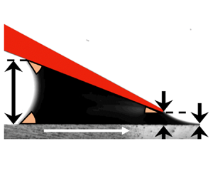
A cross-sectional view of the low-speed blade coating system is depicted in figure 1. The flow is bounded by the blade, the moving substrate and two menisci, namely the upstream meniscus between the blade and the moving substrate, and the downstream meniscus between the blade edge and the applied film surface. The coating liquid is metered by tilting the blade at angle  $\alpha$. The liquid flows through a coating gap $h_0$ between the blade and the substrate. The gap controls the amount of liquid deposited on the moving substrate, thereby serving a metering function. Meanwhile, the remainder forms a puddle between the blade and the substrate, where three three-phase contact lines are located. The advancing contact line on the substrate and the receding line under the blade are located upstream and are dynamic. The final one is downstream and is hoped to be pinned at the tip, i.e. static. As the film is deposited, the coating liquid in the puddle is exhausted continuously, causing it to shrink in size.
The cross-sectional view of non-evaporative low-speed blade coating system. Here,  $\rho$ and $\mu$ are the density and viscosity of the fluid underneath the blade, respectively, $\sigma$ is the surface tension on the gas/liquid interface, $h_{p}$, $h_0$ and $h_{w}$ are the height of the puddle, the coating gap, and the wet film thickness, respectively, $g$ is the gravitational acceleration, $\phi _{r}$ and $\phi _{a}$ are the receding and advancing contact angles, respectively, and $\alpha$ is the tilting angle of the blade.

The coating liquid was assumed to be a non-evaporative Newtonian fluid. The force balance near the coating gap determines the wet film thickness  $h_{w}$. Material properties ( $\rho$, $\mu$ and $\sigma$) and system parameters ( $g$,
$g$,  $u_{s}$, $h_{p}$, $h_0$ and $\alpha$) determine the balance. In addition to these properties and parameters, the dynamic contact angles $\phi _{r}$ and $\phi _{a}$ play a significant role in determining the size and shape of a puddle by indirectly influencing the force balance, which is a function of material properties and system parameters. The symbols’ meanings can be found in the caption of figure 1. Following the Buckingham ${\rm \pi}$ theorem, five dimensionless parameters are introduced: the dimensionless thickness $T$, the dimensionless puddle height $H_{p}$, the dimensionless edge gap $H_0$, the capillary number Ca, and the material number $m$ (Kim & Nam Reference Kim and Nam2017):
 $$\begin{gather} \displaystyle T\equiv\frac{h_{w}}{h_0},\quad H_{p}\equiv\frac{h_{p}}{\sqrt{\sigma/\rho g}},\quad H_0\equiv\frac{h_0}{\sqrt{\sigma/\rho g}},\nonumber\\ \displaystyle Ca\equiv\frac{\mu u_{s}}{\sigma},\quad m\equiv\sqrt{\frac{\rho\sigma^3}{g\mu^4}}. \end{gather}$$
As a result, the low-speed blade coating flow of non-evaporative Newtonian fluids is determined uniquely by a total of eight parameters: five dimensionless ones and three angles,  $\alpha$, $\phi _{r}$ and $\phi _{a}$. It is worth noting that the above parameters can be used to calculate the Reynolds number, which represents the competition between inertial and viscous forces:
 \begin{equation} \textit{Re} \equiv\frac{\rho u_{s}h_0}{\mu} = m H_0\,Ca. \end{equation}
In this study, we will consider the system with  $m = {O}(10^1)$, $H_0={O}(10^{-1})$ and $Ca={O}(10^{-3})$ that can be commonly encountered in a coating condition in a laboratory. As a result, $Re={O}(10^{-3})$, and the flow is described appropriately as a Stokes flow. During the coating operations, a substrate moves at a constant velocity $u_{s}$, which reduces the puddle height $h_{p}$ and, in turn, the coating thickness $h_{w}$, while all other parameters remain constant. Therefore, we concentrate primarily on the dependence of $T$ on $H_{p}$ for non-evaporative, low-Reynolds-number, capillary-dominant flows.
3. Flow visualization of blade coating flows
3.1. Experimental set-up
Figure 2 depicts a schematic of the blade coating system's experimental set-up. Silicone oil was applied to the soda-lime slide glass, which was mounted on a high-precision linear motor (V-508, Physik Instrumente GmbH & Co. KG). The physical properties of silicone oil at  $25\,^{\circ }{\rm C}$ are listed in table 1. Silicone oils are Newtonian fluids at typical laboratory temperatures and shear rates. Furthermore, the vapour pressure is low enough to ignore evaporation. To scrape the silicone oil puddle, a stainless steel blade of width 25 mm was used. The blade was sharpened so that the downstream meniscus of the oil could be pinned during coating operations.
Experimental configuration for low-speed blade coating (not to scale). The linear motor is moving in the direction indicated by the red arrow. The displacement sensor measures the wet thickness of the coated layer, and the CCD camera records the shape of the puddle for image analysis to determine the height of the puddle. (a) Side view (omit CCD camera). (b) Front view.

Physical properties of the silicone oil at  $25\,^{\circ }{\rm C}$.

As shown in figure 2, a confocal displacement sensor (CL-PT010, Keyence Co., Ltd.) was used to measure the wet thickness of the silicone oil. The wet thickness was determined indirectly by measuring the displacement of the silicone oil's free surface from the slide glass surface, which served as the reference plane. Along the centreline of the glass, the wet thickness was measured at a distance 2 mm from the blade's edge.
As depicted in the inset of figure 2(b), a CCD camera (Mako U-130B, Allied Vision Technologies GmbH) was used to record the side view of the puddle. Images obtained during flow visualizations were used to calculate the height of the puddle and the contact angles of the silicone oil.
3.2. Experimental results
The range of parameters tested in this study is summarized in table 2. The four coating speeds used are  $Ca= 0.002$, 0.004, 0.006 and 0.008, in that order. With the blade angle ${20}^{\circ }$, two different coating gaps are used. As a result, we examined eight distinct operating conditions. It should be noted that three coating experiments were performed at the same substrate speed and coating gap. Additionally, we checked the cross-web uniformity of the coated layers to ensure their flatness. This was done to validate the assumption of two-dimensional coating flows throughout the experiments.
Operating conditions for low-speed blade coating experiments.

Receding and advancing contact angles for each capillary number were measured manually and summarized in table 3. As  $Ca$ increases, the receding contact angle decreases slightly, whereas the advancing contact angle increases significantly. As a result, as $Ca$ increases, the curvature of the upstream meniscus decreases, implying a decrease in capillary force. Refer to figure 3 for details. It is important to note that the measured angles will be used as input parameters for the finite element computation and the simple viscocapillary model.
Measured dynamic contact angles for the blade coating system with  $h_0 = 300\ \mathrm {\mu }{\rm m}$.

Changes of upstream meniscus shape with respect to different  $Ca$ for the blade coating system with $h_0 = 300\ \mathrm {\mu }{\rm m}$: (a) $Ca=0.002$, (b) $Ca=0.004$, (c) $Ca=0.006$, (d) $Ca=0.008$.

The optical flow algorithm of the OpenCV library (Bradski & Kaehler Reference Bradski and Kaehler2008) was used to track the contact line on the blade as well as the substrate surface in order to extract the puddle height data from the visualization data. The algorithm produced the red markers at the upstream receding contact line, as shown in figure 3. The puddle height is then calculated by multiplying the contact line to substrate pixel distance by a pixel to length scale factor.
Despite the mechanical sharpening of the blade edge, under the following conditions, silicone oil may climb slightly above the edge, i.e. wet the upper surface of the blade edge, due to the unpinning of the downstream meniscus: fast coating speed, large puddle and narrow coating gap. When the puddle was large enough, the unpinned meniscus was observed for  $h_0=100\ \mathrm {\mu }{\rm m}$ ( $H_0 = 0.067$), as shown in figures 4(a,b). Under these conditions, both viscous stress and hydrostatic pressure may push the downstream meniscus upwards near the edge, unpinning it from the meniscus.
When the substrate moves rapidly (high  $Ca$), the gap is narrow (low $H_0$) and the puddle is large (high $H_{p}$), the contact line of the downstream meniscus can be unpinned from the blade edge, as shown in the left-hand images of (a,b). To distinguish it from the silicone oil, the blade is coloured in red. Here: (a) $Ca=0.006$, $H_0=0.067$, silicone oil wets the upper side of the blade; (b) $Ca=0.008$, $H_0=0.067$, silicone oil wets the upper side of the blade; (c) $Ca=0.002$, $H_0=0.202$, silicone oil does not wet the upper side of the blade.

Figure 5 shows dimensionless film thickness  $T$ as a function of dimensionless puddle height $H_{p}$ obtained from flow visualizations for various capillary numbers $Ca$ and coating gaps $H_0$. Unlike high-speed blade coating, wet thickness is affected by both $Ca$ and $H_{p}$. Because of the larger viscous drag that entrains the liquid, the higher the $Ca$, the thicker the film. Meanwhile, as the coating operation continues, the coating liquid in the puddle is consumed. As the puddle shrinks, the decrease in hydrostatic pressure leads to increase of the capillary pressure jump across the meniscus near the advancing contact line, and this works against viscous drag as a result.
Dimensionless film thickness  $T$ versus dimensionless puddle height $H_{p}$ for $Ca=0.002,0.004,0.006,0.008$ from flow visualizations. For each $Ca$,
$Ca$,  $H_0=0.067$ ( $h_0=100\ \mathrm {\mu }{\rm m}$) and $H_0=0.202$ ( $h_0=300\ \mathrm {\mu }{\rm m}$) are compared. The error bars represent one standard deviation. Here: (a) $Ca = 0.002$, (b) $Ca = 0.004$, (c) $Ca = 0.006$, (d) $Ca = 0.008$.

In the next section, we will introduce two-dimensional finite element computations to predict the wet thickness that can be compared directly to the experimental results.
4. Computational approach
4.1. Finite element computations
A notable geometrical feature of typical coating flows is a significantly high aspect ratio, which means that a length scale in the cross-web or cross-substrate direction is significantly greater than the other two length scales. Furthermore, the requirement for uniformity in wet thickness favours vanishing cross-flows away from edges. Otherwise, there will be thickness variations in the cross-web direction. As a result, we consider the blade coating flow to be two-dimensional. This flow represents flow away from the edges in the substrate width direction in the midplane.
We used a system of equations for the two-dimensional blade coating flow, and solved it numerically using the Galerkin finite element method in this study. The flow domain is depicted in figure 1. The arbitrary Lagrangian–Eulerian (ALE) method was also used to solve the free boundary problem caused by the two gas/liquid interfaces.
4.1.1. Governing equations and boundary conditions
The low-speed blade coating flow is governed by the mass and momentum balance equations
 \begin{gather} \boldsymbol{\nabla}^*\boldsymbol{\cdot}\boldsymbol{u}^*=0, \end{gather}
 \begin{gather}\rho\left(\frac{\partial{\boldsymbol{u}^*}}{\partial{t^*}}+\boldsymbol{u}^*\boldsymbol{\cdot}\boldsymbol{\nabla}^*\boldsymbol{u}^*\right)=\boldsymbol{\nabla}^*\boldsymbol{\cdot}\boldsymbol{\mathsf{T}}^*+\rho\boldsymbol{g}, \end{gather}
where  $\boldsymbol {u}^*$ is the velocity field, $\boldsymbol {g}$ is the gravitational field, and $\boldsymbol{\mathsf{T}}^*$ is the total stress tensor for Newtonian fluids defined by
 \begin{equation} \boldsymbol{\mathsf{T}}^*={-}p^*\boldsymbol{\mathsf{I}}+\mu\left[\boldsymbol{\nabla}^*\boldsymbol{u}^*+\left(\boldsymbol{\nabla}^*\boldsymbol{u}^*\right)^{{\rm T}}\right]\!. \end{equation}
Figure 6 summarizes the boundary conditions considered in this study. The no-slip conditions apply to the moving substrate as well as the blade surface:
 \begin{gather} \boldsymbol{u}^*=\boldsymbol{u}_{s}\quad\text{on the moving substrate}, \end{gather}
 \begin{gather}\boldsymbol{u}^*=\boldsymbol{0}\quad\text{on the blade wall}. \end{gather}
Flow domain and boundary conditions for the low-speed blade coating flow. The unit normal and tangent vector definitions are shown.

As stated previously, the downstream contact line is pinned at the blade edge during the desirable coating operations. To reduce the complexity of the computational model, therefore, we assumed that the contact line is pinned:
 \begin{equation} \boldsymbol{x}^*=\boldsymbol{x}_{p}. \end{equation}
However, the coating liquid may wet over the blade edge, as observed in § 3.2 for certain conditions.
Two contact lines moving upstream must be handled with care to avoid a non-integrable singularity in shear stress caused by the velocity discontinuity (Huh & Scriven Reference Huh and Scriven1971). We use the Navier slip condition with constant dynamic contact angles  $\phi$, as described in Romero & Carvalho (Reference Romero and Carvalho2008):
 \begin{gather} \beta\boldsymbol{t}_{w}\boldsymbol{n}_{w}:\boldsymbol{\mathsf{T}}^*=\boldsymbol{t}_{w}\boldsymbol{\cdot}\left(\boldsymbol{u}^*-\boldsymbol{u}_{s}\right)\!, \end{gather}
 \begin{gather}\boldsymbol{n}_{m}\boldsymbol{\cdot}\boldsymbol{n}_{w}={-}\cos\phi, \end{gather}
where  $\boldsymbol {n}_w$ and $\boldsymbol {t}_w$ are unit normal and tangent vectors of the wall defined as in figure 6. Here, $\beta$ is the empirical slip coefficient, chosen as $\beta =0.1\,{\rm g}^{-1}\,{\rm mm}^2\,{\rm s}$. The values of $\phi$ for advancing and receding contact angles are measured from flow visualization results and summarized in table 3.
This flow system features a synthetic outflow boundary in which a moving substrate translates a thin film. The velocity profile at the boundary was unknown a priori, so we imposed the free boundary condition proposed by Papanastasiou, Malamataris & Ellwood (Reference Papanastasiou, Malamataris and Ellwood1992):
 \begin{equation} \boldsymbol{n}_{b}\boldsymbol{\cdot}\boldsymbol{\mathsf{T}}^*={-}\boldsymbol{n}_{b}\,p^*+\boldsymbol{n}_{b}\boldsymbol{\cdot}\mu\left[\boldsymbol{\nabla}^*\boldsymbol{u}^*+\left(\boldsymbol{\nabla}^*\boldsymbol{u}^*\right)^\mathrm{T}\right]\!. \end{equation}
This boundary condition appears to impose nothing. Renardy (Reference Renardy1997), on the other hand, demonstrated that the condition ensures well-posedness at the discretization level, particularly for a nearly fully developed flow.
The size of the flow domain at the outlet, i.e. the height of the outlet, is also unknown at the outflow boundary. In this case, the height is proportional to the film thickness as determined by the force balance within the coating flow (Ruschak Reference Ruschak1985). Furthermore, the downstream meniscus is forced to be perpendicular to the outflow boundary to prevent undesirable mesh distortion at the end of the meniscus:
 \begin{equation} \boldsymbol{n}_{m}\boldsymbol{\cdot}\boldsymbol{n}_{b}=0. \end{equation}
This condition appears to fail when the outflow boundary is close to the blade edge, as the thickness profile may decrease significantly along the flow direction. Therefore, the outflow boundary is placed far away from the blade edge to reduce any numerical artefacts caused by this condition. This distance is set to thirty times the coating gap in this study.
The flow domain is deformable, comprising three fixed boundaries and two deformable ones, i.e. menisci. In this study, the domain is discretized into quadrilateral finite elements, whose nodal positions are unknown a priori. Thus the governing equations and boundary conditions on the physical domain  $\boldsymbol {x}^*=(x^*,y^*)$ should be mapped into the fixed reference domain $\boldsymbol {\xi }=(\xi,\eta )$ by $\boldsymbol {x}^*=\boldsymbol {F}(\boldsymbol {\xi })$. The inverse transformation $\boldsymbol {F}^{-1}$ is a solution of elliptic partial differential equations
 \begin{equation} \boldsymbol{\nabla}^*\boldsymbol{\cdot}\boldsymbol{D}\boldsymbol{\cdot}\boldsymbol{\nabla}^*\boldsymbol{\xi}=\boldsymbol{0}, \end{equation}
where  $\boldsymbol {D}\equiv (D_\xi,D_\eta )$ is mesh diffusivity, which controls the nodal spacing in equipotential curves of $\xi$ and $\eta$ in the physical domain. Those curves and their intersects define boundaries and nodes of quadrilateral elements in the physical domain (de Santos Reference de Santos1991).
On the upstream and downstream menisci, the stress balance as well as the kinematic conditions should be imposed:
 \begin{gather} \boldsymbol{n}_{m}\boldsymbol{\cdot}\boldsymbol{\mathsf{T}}^*=\sigma\kappa^*\boldsymbol{n}_{m}, \end{gather}
 \begin{gather}\frac{\partial{M}}{\partial{t^*}}+\boldsymbol{u}^*\boldsymbol{\cdot}\boldsymbol{\nabla}^*M=0, \end{gather}
where  $\boldsymbol {n}_{m}$ is the outward unit normal vector of the meniscus, $\kappa ^*=-\boldsymbol {\nabla }^*\boldsymbol {\cdot }\boldsymbol {n}_{m}$ is the curvature of the meniscus, and $M\equiv \xi (x^*,y^*)+C$, where $C$ is a constant. In our ALE formulation, $M=0$ is the equipotential curve for free surfaces. These coupled conditions allow the mesh boundary to track the free surface precisely.
In the ALE-formulated transient flow system considered in this study, nodal points in the physical domain governed by (4.11) move through time. As a result, the frame of reference should be transformed using total derivatives from fixed Eulerian  $x^*, y^*$ coordinates to fixed iso-parametric $\xi, \eta$ coordinates, as described by Christodoulou & Scriven (Reference Christodoulou and Scriven1992):
 \begin{equation} \frac{\partial{f^*}}{\partial{t^*}}={\mathop {f^*}\limits^\circ}-{\mathop {\boldsymbol{x^*}}\limits^\circ} \boldsymbol{\cdot}\boldsymbol{\nabla}^*f^*, \end{equation}
where  ${\mathop {f^*}\limits^\circ}$ denotes the time derivative of an arbitrary field variable $f$ at fixed iso-parametric coordinates, so ${\mathop {\boldsymbol{x^*}}\limits^\circ}$ is interpreted as the mesh velocity. Consequently, the momentum balance (4.2) and the kinematic condition (4.13) become
 \begin{gather} \rho\left[{\mathop {\boldsymbol{u^*}}\limits^\circ}+\left(\boldsymbol{u}^*-{\mathop {\boldsymbol{x^*}}\limits^\circ}\right)\boldsymbol{\cdot}\boldsymbol{\nabla}^*\boldsymbol{u}^*\right]=\boldsymbol{\nabla}^*\boldsymbol{\cdot}\boldsymbol{\mathsf{T}}^*+\rho\boldsymbol{g}, \end{gather}
 \begin{gather}\boldsymbol{n}_{m}\boldsymbol{\cdot}\left(\boldsymbol{u}^*-{\mathop {\boldsymbol{x^*}}\limits^\circ}\right)=0, \end{gather}
respectively. Finally, the governing equations (4.1), (4.11) and (4.15) are solved simultaneously with proper boundary conditions to determine field variables including position, velocity and pressure.
4.1.2. Solution methods
The finite element method (FEM) approximates field variables as linear combinations of basis functions in the iso-parametric reference domain:
 \begin{equation} \boldsymbol{x}^*=\sum_{i=1}^n \boldsymbol{x}_i^*(t^*)\,\phi_i(\xi,\eta),\quad\boldsymbol{u}^*=\sum_{i=1}^n \boldsymbol{u}_i^*(t^*)\,\phi_i(\xi,\eta),\quad p^*=\sum_{i=1}^m p_i^*(t^*)\,\psi_i(\xi,\eta), \end{equation}
where  $\phi _i(\xi,\eta )$ are Lagrangian biquadratic functions and $\psi _i(\xi,\eta )$ are linear discontinuous functions. The coefficients $\boldsymbol {x}^*_i(t^*),\ \boldsymbol {u}^*_i(t^*)$ and $p_i^*(t^*)$ are the time-dependent nodal values of the field variables to be solved.
The governing equations are multiplied by weighting functions (basis functions in the Galerkin FEM) and integrated over the physical domain. The weighted residuals and their weak forms are described specifically in Romero & Carvalho (Reference Romero and Carvalho2008). Finally, the governing equations are reduced to a system of nonlinear algebraic equations
 \begin{equation} \boldsymbol{R}\left(\boldsymbol{z},{\mathop {z}\limits^\circ},\boldsymbol{\lambda}\right)=\boldsymbol{0}, \end{equation}
where  $\boldsymbol {z}$ is the solution vector consisting of unknown coefficients of the basis functions, and ${\mathop {z}\limits^\circ}$ contains their time derivatives. The vector $\boldsymbol {\lambda }$ consists of known system parameters such as material and geometrical properties.
Utilizing a predictor–corrector algorithm, the evolution of the temporally discrete system (4.18) is managed. The predictor step provides a good initial guess for the corrector step, which employs implicit time integration methods. Except for the first and second time steps, the predictor–corrector pair consists of the second-order Adams–Bashforth (AB2) method and the second-order trapezoid rule (TR) method:
 \begin{gather} \text{AB2}\quad\boldsymbol{z}_{n+1}^{p} = \boldsymbol{z}_n + \frac{3\Delta t^*}{2}\,{\mathop {z}\limits^\circ}_n - \frac{\Delta t^*}{2}\,{\mathop {z}\limits^\circ}_{n-1}, \end{gather}
 \begin{gather}\text{TR}\quad {\mathop {z}\limits^\circ}_{n+1}=\frac{2}{\Delta t^*}\left(\boldsymbol{z}_{n+1}-\boldsymbol{z}_n\right)- {\mathop {z}\limits^\circ}_n, \end{gather}
where the superscript  ${p}$ refers to the solution vector obtained from the predictor step, and $\Delta t^*$ is a fixed time increment. The first-order backward Euler (BE) method is adopted to solve the first time step:
 \begin{equation} \mbox{BE}\quad {\mathop {z}\limits^\circ}_{n+1}=\frac{\boldsymbol{z}_{n+1}-\boldsymbol{z}_n}{\Delta t^*}. \end{equation}
Then TR followed by the forward Euler (FE) method are applied in the second time step:
 \begin{equation} \mbox{FE}\quad\boldsymbol{z}_{n+1}^{p} = \boldsymbol{z}_n + \Delta t^*\,{\mathop {z}\limits^\circ}_n. \end{equation}
In the corrector step, Newton's method is used to solve the system of nonlinear equations for each time step:
 \begin{gather} \left. \begin{array}{c@{}} \displaystyle\left[\boldsymbol{\mathsf{J}}_{\boldsymbol{R}}^{BE}\left(\boldsymbol{z}_{1}^k,\boldsymbol{\lambda}_{1}\right)+\dfrac{1}{\Delta t^*}\,\boldsymbol{\mathsf{M}}_{\boldsymbol{R}}^{BE}\left(\boldsymbol{z}_{1}^k,\boldsymbol{\lambda}_{1}\right)\right]\delta\boldsymbol{z}_{1}^k={-}\boldsymbol{R}^{BE}\left(\boldsymbol{z}_{1}^k,\boldsymbol{\lambda}_{1}\right),\\ \boldsymbol{z}_{1}^{k+1} = \boldsymbol{z}_{1}+\delta\boldsymbol{z}_{0}^k, \end{array} \right\} \end{gather}
 \begin{gather}\left. \begin{array}{c@{}} \displaystyle\left[\boldsymbol{\mathsf{J}}_{\boldsymbol{R}}^{TR}\left(\boldsymbol{z}_{n+1}^k,\boldsymbol{\lambda}_{n+1}\right)+\dfrac{2}{\Delta t^*}\,\boldsymbol{\mathsf{M}}_{\boldsymbol{R}}^{TR}\left(\boldsymbol{z}_{n+1}^k,\boldsymbol{\lambda}_{n+1}\right)\right]\delta\boldsymbol{z}_{n+1}^k ={-}\boldsymbol{R}^{TR}\left(\boldsymbol{z}_{n+1}^k,\boldsymbol{\lambda}_{n+1}\right), \\ \boldsymbol{z}_{n+1}^{k+1} = \boldsymbol{z}_{n+1}+\delta\boldsymbol{z}_{n+1}^k\quad (n\ge1), \end{array} \right\} \end{gather}
where  $\boldsymbol{\mathsf{J}}_{\boldsymbol {R}}\equiv \partial \boldsymbol {R}/\partial \boldsymbol {z}$ and $\boldsymbol{\mathsf{M}}_{\boldsymbol {R}}\equiv \partial \boldsymbol {R}/\partial {\mathop {z}\limits^\circ}$ are the Jacobian matrix and the mass matrix, respectively. The superscripts BE and TR denote the different kinds of applied temporal discretizations. The tolerance for the Newton iteration is set to $\lVert \boldsymbol {R}(\boldsymbol {z}_{n+1}^k,\boldsymbol {\lambda }_{n+1})\rVert _2 < 10^{-9}$.
In this study, transient computation was initiated with a steady-state solution rather than a static pool of the puddle behind the blade without a downstream film section. If the static pool is chosen as a starting point, then managing the growth of the downstream film section becomes necessary. However, re-meshing may be necessary due to the significant deformation of elements caused by the ALE approach, which can impact negatively the accuracy of the computed solutions.
Due to the continuous outflow, the blade coating system considered in this study will never reach a steady state. In contrast, steady-state blade coating systems can be computed in the case of continuous inflow, as demonstrated by Lee et al. (Reference Lee, Lee, Lee, Ahn, Nam and Park2020). To accommodate this approach, we added an artificial inflow boundary on the blade lower surface  $h_0/2$ away from the blade edge, as indicated by the red arrow in figure 7. The inflow boundary has size $h_0/2$. The effect of artificial boundaries must be reduced for transient computations. Therefore, the velocity profile at the boundary was designed to decrease the flow rate linearly:
 \begin{equation} \boldsymbol{u}^*= \left\{ \begin{array}{ll} \displaystyle \dfrac{6q}{w_{i}}\left[\left(\dfrac{s^*}{w_{i}}\right)-\left(\dfrac{s^*}{w_{i}}\right)^2\right]\left(1-\dfrac{n}{50}\right)(-\boldsymbol{n}_{w}), & 0\le n < 50,\\ \boldsymbol{0}, & n\ge 50, \end{array}\right. \end{equation}
where  $q$ is the flow rate per width, which in the steady state is equal to $h_{w}u_{s}$ due to mass conservation. Here, $w_{i}$ is the width of the inlet, $s^*$ is the local coordinate of the inflow boundary ( $0\le s^*\le w_{i}$), and $n$ is the time step used in (4.19)–(4.24). It is important to note that (4.25) guarantees the deactivation of the artificial inlet flow after 50 time steps.
Configuration of the mesh and streamlines of the steady-state solution at  $\alpha ={20}^{\circ }$, $m=12.94$, $Ca=0.002$, $H_0=0.202$, $T=0.3$, $H_{p}=1.356$, $\phi _{r}={40.3}^{\circ }$ and $\phi _{a}={42.7}^{\circ }$, where 3100 quadrilateral elements are used to discretize the flow domain. The artificial inflow boundary is indicated by the thick red arrow and the details on the inflow velocity profile are shown below. Note that the inlet boundary transitions into a standard no-slip wall after 50 initial time steps.

The mesh configuration and streamlines of the initial steady-state solution of the base case with  $\alpha ={20}^{\circ }$, $m=12.94$ (silicone oil, see table 1), $Ca=0.002$, $H_0=0.202$ ( $h_0=300\ \mathrm {\mu }\textrm {m}$) and $T=0.3$ are shown in figure 7. The values reported in table 3 were used for the receding and advancing contact angles. The dimensionless puddle height $H_{p}$ is calculated to be 1.356. Using the first-order natural continuation (Bolstad & Keller Reference Bolstad and Keller1986) of relevant parameters, steady-state solutions were computed with different operating conditions.
4.2. Computational results
The time increment  $\Delta t^*$ is set to $0.05/u_{s}$, where the unit of $u_{s}$ is $\textrm {mm}\ \textrm {s}^{-1}$. In other words, the substrate translates $50\ \mathrm {\mu }\textrm {m}$ in a single time step.
According to the experimental results, the film thickness decreases gradually over time. As shown in figure 8, our numerical solutions produce a typical long-wave pattern on a film profile. The minimum height of the film profile at each time step is chosen as the wet thickness  $h_{w}$. As the puddle height $h_{p}$ decreases or the time passes, the location of the minimum height moves upstream, and the wet thickness decreases.
Temporal evolution of the downstream menisci profiles from  $H_{p}=1.184$ (dark blue line) to $H_{p}=0.3200$ (dark red line), scaled by $h_0$. The time difference between two adjacent profiles is $\Delta t^*=11.502\ \textrm {s}$. The cross markers indicate the minimum height locations, which are regarded as film thickness at the time.

The results of transient computations are shown in figure 9. All computations began with the initial steady state using  $H_{p}\sim 1.4$. To reduce the numerical artefacts caused by the artificial inflow condition, at least the first 250 steps of computed solutions were discarded. It is worth noting that $H_{p}$ decreases over time.
Dimensionless wet thickness  $T$ was calculated as a function of dimensionless puddle height $H_{p}$ for different capillary numbers $Ca$ and dimensionless coating gaps $H_0$. The blade tilt angle is set to $\alpha ={20}^{\circ }$. The range of $H_{p}$ is set approximately to $1.1H_0(1+\tan \alpha )< H_{p}<1.2$. Here: (a) $Ca = 0.002$, (b) $Ca = 0.004$, (c) $Ca = 0.006$, (d) $Ca = 0.008$.

As the silicone oil is drained from the puddle during the blade coating process, the thickness of the film decreases, which is consistent with the experimental observations. The numerical results further indicate an increase in  $T$ as a result of higher viscous drag caused by high $Ca$. In addition, the narrow coating gap leads to a thicker film in a dimensionless sense. The next section will introduce a theoretical model to examine these findings in greater depth.
Figure 10 compares the computational and experimental results. Generally, the predicted thickness matches the measured thickness accurately in some parameter ranges, such as the small  $H_{p}$, large $H_0$, or small $Ca$ regimes. The disparity between the thickness $T$ obtained from computations and experiments increases with greater puddle height $H_{p}$. Two causes explain the discrepancy.
Comparison of experimental results (markers with error bars) and numerical computation (dashed lines) for  $H_0=0.067$ (blue) and $H_0=0.202$ (red). Except for $H_0=0.067$ with $Ca=0.004$, 0.006 and $0.008$, where the silicone oil was not pinned at the blade edge, the two-dimensional computation slightly overestimates the wet thickness, as shown in § 3.2. Here: (a) $Ca = 0.002$, (b) $Ca = 0.004$, (c) $Ca = 0.006$, (d) $Ca = 0.008$.

First, two-dimensional computations cannot account for three-dimensional flow features, such as swollen coated film edges caused by outward flow towards edges. This flow reduces the thickness of the film in the interior film region, where the displacement sensor is aimed. As a result, the thickness predicted by the computations should be greater than the thickness measured by the experiments, as shown in the  $H_0=0.202$ cases of figure 10. This edge effect is common in other coating flows, such as slot coating (Schmitt, Scharfer & Schabel Reference Schmitt, Scharfer and Schabel2014).
Another factor is associated with the meniscus pinning at the blade edge. During computations, the meniscus pinning is related to the boundary condition where the extreme point of the downstream meniscus is fixed at the blade edge. However, according to § 3.2, silicone oil tends to wet the upper side of the blade during high-speed operations when the coating gap is narrow. This ‘unwanted’ edge wetting increases the measured wet film thickness due to an effective increase in the coating gap. The degree of edge wetting rises with the pressure near the edge, which can be increased by either raising the viscous drag (high  $Ca$) or reducing the coating gap (low $H_0$). As a result, the discrepancy between computations and experiments increases as $Ca$ rises or $H_0$ diminishes. The cases $Ca=0.006$ and $0.008$ with $H_0=0.067$ in figure 10 highlight this effect.
To focus on the effects that govern wet film thickness, we limited our study to two-dimensional phenomena, since the precise modelling of swollen edges and edge unpinning in three dimensions is challenging. In the next section, we propose a simple viscocapillary model for low-speed blade coating flows. This model provides insight into the nonlinear change in thickness that occurs as the puddle height decreases.
5. Viscocapillary model
5.1. Construction of a simple viscocapillary model
Under the assumption that the coating flow evolves slowly (i.e. in the quasi-steady state) and the speed of the operations is sufficiently low to ignore the inertial force ( $Re=mH_0\,Ca\ll 1$), a viscocapillary model for low-speed blade coating can be proposed. As a result, the momentum balance equation (4.2) can be simplified to the Stokes equation:
 \begin{equation} \boldsymbol{0} = \boldsymbol{\nabla}^*\boldsymbol{\cdot}\boldsymbol{\mathsf{T}}^*+\rho\boldsymbol{g}. \end{equation}
On the moving substrate and the blade wall, the boundary conditions (4.4)–(4.6) are applied. Two menisci are subjected to the stress balance (4.12). The kinematic condition (4.13) on the menisci, on the other hand, is simplified as
 \begin{equation} \boldsymbol{n}_{m}\boldsymbol{\cdot}\boldsymbol{u}^*=0, \end{equation}
due to the quasi-steady state assumption.
The proposed viscocapillary model for low-speed blade coating divides the flow domain into three regions, as illustrated in figure 11. In the upstream meniscus region I, the pressure jump across the gas/liquid interface is taken into account. The pressure field in the convergent channel region II is affected significantly by the channel shape, particularly near the blade edge. The film formation region III exhibits flow characteristics similar to the drag-out problem in dip coating, which was pioneered by Landau & Levich (Reference Landau and Levich1942). To compute the field variables such as pressure, the model treats these regions separately, then patches them together using pressure-matching conditions. Finally, the wet film thickness in the film formation region is calculated using the film profile equation.
The low-speed blade coating system can be divided into three regions: the upstream meniscus region I, the convergent channel region II, and the film formation region III.

5.1.1. Upstream meniscus region
The upstream meniscus region can be simplified greatly to the static meniscus under the quasi-steady state assumption. Because  $h_{p}$ is chosen as the characteristic length, the dimensionless variables for the upstream meniscus region become
 \begin{equation} x^*=h_{p}\tilde x,\quad y^*=h_{p}\tilde y,\quad\kappa^*=\frac{\tilde\kappa}{h_{p}},\quad p^*=\frac{\sigma}{h_{p}}\,\tilde p. \end{equation}
The shape of the approximated quiescence meniscus is governed by the Young–Laplace equation. Utilizing the contact angles as boundary conditions, the capillary pressure jump across the meniscus can be derived, as shown in Yim & Nam (Reference Yim and Nam2022):
 \begin{equation} \tilde p\left(\tilde y\right) ={-}\tilde\kappa\left(\tilde y\right) ={-}H_{p}^2\tilde y+\frac{H_{p}^2}{2}-\tilde\kappa_{m0}, \end{equation}
where  $\tilde \kappa _{m0}$ represents the curvature in the absence of gravity,
 \begin{equation} \tilde\kappa_{m0}=\cos\left(\alpha+\phi_{r}\right) + \cos\phi_{a}. \end{equation}
As the matching condition, the pressure at the receding contact line  $\tilde p(\tilde y=1)$ will be used as the pressure datum for the convergent channel region.
5.1.2. Convergent channel region
The two-dimensional flow is driven by the moving boundary in this wedge-shaped region, with leakage due to film entrainment. Because the Stokes equation is used to describe the flow in this region, we use the stream function  $\psi ^*$ in polar coordinates, as shown in figure 12:
 \begin{equation} u_r^*\equiv{-}\frac{1}{r^*}\,\frac{\partial{\psi^*}}{\partial{\theta}},\quad u_\theta^*\equiv\frac{\partial{\psi^*}}{\partial{r^*}}. \end{equation}
Taking the curl of the Stokes equation followed by substituting the stream function yields the biharmonic equation
 \begin{equation} \nabla^{*4}\psi^*(r^*,\theta)=0. \end{equation}
The solutions of this equation could be represented in a separable form:
 \begin{equation} \psi^*(r^*,\theta) = Ar^{*\lambda}\,f(\theta), \end{equation}
where  $A$ is a prefactor and $\lambda$ is a real or complex number.
The convergent channel region in polar coordinates.

Following Riedler & Schneider (Reference Riedler and Schneider1983), a superposition of two distinct solutions is used to describe the flow in a corner with leakage:
 \begin{equation} \psi^*=\psi_1^*+\psi_2^*={-}u_{s}r^*\,f_1(\theta)-q\,f_2(\theta), \end{equation}
where  $\psi _1^*$ represents flow in a corner with a sliding boundary, also known as Taylor scraping flow, $\psi _2^*$ describes leakage from the point sink, i.e. the origin in figure 12, and $q$ is sink strength, which is equal to $h_{w}u_{s}$ due to mass conservation. To satisfy no-slip at the wall as well as the constant leakage to the origin, $f_1(\theta )$ and $f_2(\theta )$ in the stream function must satisfy the boundary conditions
 \begin{equation} \left. \begin{gathered} f_1=0,\quad f'_1={-}1,\quad f_2=0,\quad f'_2=0\quad\text{at}\ \theta=0, \\ f_1=0,\quad f'_1=0,\quad f_2={-}1,\quad f'_2=0\quad\text{at}\ \theta=\alpha. \end{gathered} \right\} \end{equation}
The flow can be described using the dimensionless variable definitions
 \begin{equation} r^*=h_0\,r,\quad\psi^*=h_0u_{s}\,\psi,\quad u_r^*=u_{s}\,u_r,\quad u_\theta^*=u_{s}\,u_\theta,\quad p^*=\frac{\sigma}{h_{p}}\, p_{c}. \end{equation}
Solving (5.7) by substituting (5.9) with boundary conditions (5.10) followed by non-dimensionalization yields
 \begin{equation} \psi(r,\theta) = r\,\frac{-\theta\sin\alpha\sin2(\alpha-\theta)+\alpha(\alpha-\theta)\sin\theta}{\alpha^2-\sin^2\alpha} +T\,\frac{\theta\cos\alpha-\cos(\alpha-\theta)\sin\theta}{\alpha\cos\alpha-\sin\alpha}. \end{equation}
 Now the pressure field  $p_{c}$ can be obtained from the scaled momentum equation with the velocity field $u_r$ or $u_\theta$ obtained from the stream function above:
 \begin{equation} \left. \begin{gathered} \displaystyle-\frac{H_0}{H_{p}}\,\frac{\partial{p_{c}}}{\partial{r}}+Ca\left[\frac{\partial{}}{\partial{r}}\left(\frac{1}{r}\,\frac{\partial{}}{\partial{r}}\left(ru_r\right)\right)+\frac{1}{r^2}\,\frac{\partial^{2}{u_r}}{\partial{\theta}^{2}}-\frac{2}{r^2}\,\frac{\partial{u_\theta}}{\partial{\theta}}\right]-H_0^2\sin\theta=0, \\ \displaystyle-\frac{H_0}{rH_{p}}\,\frac{\partial{p_{c}}}{\partial{\theta}}+Ca\left[\frac{\partial{}}{\partial{r}}\left(\frac{1}{r}\,\frac{\partial{}}{\partial{r}}\left(ru_\theta\right)\right)+\frac{1}{r^2}\,\frac{\partial^{2}{u_\theta}}{\partial{\theta}^{2}}+\frac{2}{r^2}\,\frac{\partial{u_r}}{\partial{\theta}}\right]-H_0^2\cos\theta=0. \end{gathered} \right\} \end{equation}
Using the pressure at the receding contact line, the pressure datum is determined by matching the upstream meniscus region and this region:
 \begin{equation} p_{c}\left(\frac{H_{p}}{H_0\sin\alpha}, \alpha\right)=\tilde p(\tilde y=1). \end{equation}
Finally, the pressure at the blade edge  $\tilde p_{c0}$ can be calculated as
 \begin{equation} p_{c0}\equiv p_{c}\left(\frac{1}{\sin\alpha}, \alpha\right) = p_{c}^{c} + p_{c}^{h} + p_{c}^{g} + p_{c}^{l}, \end{equation}
where
 \begin{equation} \left. \begin{gathered} \displaystyle p_{c}^{c}={-}\frac{H_{p}^2}{2}-\tilde\kappa_{m0},\quad p_{c}^{h}=H_{p}^2(1-R),\\ \displaystyle p_{c}^{g}=\frac{Ca\,(1-R)}{R}\,\frac{2\alpha\sin^2\alpha}{\alpha^2-\sin^2\alpha}, \\ \displaystyle p_{c}^{l}={-}\frac{Ca\,(1-R^2)}{R}\,\frac{2T\cos\alpha\sin^2\alpha}{\sin\alpha-\alpha\cos\alpha}, \end{gathered} \right\} \end{equation}
with  $p_{c}^{c}, p_{c}^{h}, p_{c}^{g}, p_{c}^{l}$ representing the capillary pressure at the receding contact line, the hydrostatic pressure between the receding contact line and the blade edge, the pressure growth due to the convergent channel, and the pressure drop due to the leakage, respectively.
Here, we introduce an additional dimensionless parameter, called the gap to puddle height ratio, which can be expressed as
 \begin{equation} R = \frac{h_0}{h_p} = \frac{H_0}{H_{p}}. \end{equation}
 As the puddle is drained, this ratio approaches unity, which can indicate the progress of coating for a given  $H_0$. The pressure at the blade edge, $p_{c0}$, will be used to determine the matching condition between this region and the film formation region.
5.1.3. Film formation region
In the film formation region, the film is formed from the downstream meniscus, as its name suggests. The balance among viscous, capillary and gravitational forces determines the film profile or shape of the gas/liquid interface. The flow system in this region is analogous to the Landau–Levich problem, with the exception that gravity acts perpendicular to the moving substrate. Therefore, the curvature-matching method of Landau & Levich (Reference Landau and Levich1942) can be utilized to determine the film thickness  $T$ for low $Ca$ flows.
Figure 13 presents a schematic of the film formation region, which can be further divided into three subregions. Near the blade edge, where flow is minimal, the meniscus can be assumed to be static, with the meniscus shape determined by the equilibrium between capillary and gravitational forces. The positive curvature in this static meniscus subregion leads to a significant reduction in the film thickness. In the dynamic meniscus subregion, the viscous drag from the moving substrate cannot be ignored and are considered in the force balance to determine the shape. The curvature and velocity gradient decrease in this region, and the film profile changes gradually. Ultimately, all forces become balanced, and the film is entrained by the moving substrate in the film entrainment subregion, where the film profile is flat.
Three flow subdomains in the film formation region. The outward unit normal vector is defined as  $\boldsymbol {n}_{m}=(-{h^*}'\boldsymbol {i}+\boldsymbol {j})/\sqrt {1+{h^*}''}.$ It should be noted that the subregions are not scaled.

Following Park & Homsy (Reference Park and Homsy1984), the variables for the static and dynamic meniscus regions are non-dimensionalized by appropriate scales, respectively:
 \begin{equation} \left. \begin{gathered} x^*=h_0 x,\quad y^*=h_0y,\quad h^*=h_0h, \\ \displaystyle u_x^*=u_{s}u_x,\quad u_y^*=u_{s}u_y,\quad p^*=\frac{\sigma}{h_0}\,p \end{gathered} \right\} \end{equation}
and
 \begin{equation} \left. \begin{gathered} x^*=h_0\, Ca^{1/3} \,\bar x,\quad y^*=h_0\, Ca^{2/3}\, \bar y,\quad h^*=h_0\,Ca^{2/3}\,\bar h,\\ \displaystyle u_x^*=u_{s}\bar u_x,\quad u_y^*=u_{s}\, Ca^{1/3}\, \bar u_y,\quad p^*=\frac{\sigma}{h_0}\,\bar p. \end{gathered} \right\} \end{equation}
Scaled variables in the static meniscus subregion are denoted by dropping the asterisks like variables in the convergent channel region (5.11a–e), whereas scaled variables in the dynamic meniscus region are denoted by overbars.
When the capillary number  $Ca$ is sufficiently low ( $Ca^{1/3}\ll 1$), the Stokes equation (5.1) and the stress balance condition (4.12) in the static meniscus region can be reduced in terms of $Ca^{1/3}$ using the leading-order approximation:
 \begin{gather} \frac{\mathrm{d}^{}{p}}{\mathrm{d}^{}{y}}+H_0^2=0, \end{gather}
 \begin{gather}p={-}\frac{\mathrm{d}^{2}{h}}{\mathrm{d}\kern 0.06em {x}^{2}}\left[1+\left(\frac{\mathrm{d}{h}}{\mathrm{d}\kern 0.06em {x}}\right)^2\right]^{{-}3/2}\quad\text{at}\
y=h(x). \end{gather}
\begin{gather}p={-}\frac{\mathrm{d}^{2}{h}}{\mathrm{d}\kern 0.06em {x}^{2}}\left[1+\left(\frac{\mathrm{d}{h}}{\mathrm{d}\kern 0.06em {x}}\right)^2\right]^{{-}3/2}\quad\text{at}\
y=h(x). \end{gather}
Integrating (5.21) requires a boundary condition. As the pressure datum boundary condition, we use the pressure at the edge obtained from the convergent region, (5.15).
As we will discuss later, the matching procedure employed in this study may lead to order inconsistency in  $Ca$ due to the absence of $Ca$ in (5.20) and (5.21), while $p_{c0}$ contains $Ca\,(1-R)/R$ in $p_{c}^{g}$ and $p_{c}^{l}$. Thus, depending on the puddle height $R$, this inconsistency may affect the accuracy of the computed thickness. Despite this issue, we adopted this matching condition for its practicality, albeit at the expense of mathematical rigour.
Using the matching condition via the pressure datum, the film profile equation for the static meniscus becomes
 \begin{equation}
\frac{\mathrm{d}^{2}{h}}{\mathrm{d}\kern 0.06em {x}^{2}}\left[1+\left(\frac{\mathrm{d}{h}}{\mathrm{d}\kern 0.06em {x}}\right)^2\right]=H_0^2(h-1)-R\,p_{c0}.
\end{equation}
\begin{equation}
\frac{\mathrm{d}^{2}{h}}{\mathrm{d}\kern 0.06em {x}^{2}}\left[1+\left(\frac{\mathrm{d}{h}}{\mathrm{d}\kern 0.06em {x}}\right)^2\right]=H_0^2(h-1)-R\,p_{c0}.
\end{equation}
In the dynamic meniscus region under  $Ca^{1/3}\ll 1$, the leading-order equations for the governing equations and boundary conditions are
 \begin{gather} \frac{\partial{\bar u_x}}{\partial{\bar x}} + \frac{\partial{\bar u_y}}{\partial{\bar y}} = 0, \end{gather}
 \begin{gather}-\frac{\mathrm{d}{\bar p}}{\mathrm{d}{\bar x}} + \frac{\partial^{2}{\bar u_x}}{\partial{\bar y}^{2}} = 0, \end{gather}
 \begin{gather}\bar u_x = 1, \bar u_y = 0\quad\mbox{at}\ \bar y=0, \end{gather}
 \begin{gather}\left. \begin{array}{c@{}} \displaystyle\dfrac{\partial{\bar u_x}}{\partial{\bar y}}=0, \\ \displaystyle\bar p ={-}\dfrac{\mathrm{d}^{2}{\bar h}}{\mathrm{d}{\bar x}^{2}} \end{array}\right\}\quad\mbox{at}\ \bar y=\bar h(\bar x), \end{gather}
 \begin{gather}-\bar u_x\,\frac{\mathrm{d}{\bar h}}{\mathrm{d}{\bar x}}+\bar u_y = 0\quad\mbox{at}\ \bar y=\bar h(\bar x). \end{gather}
The  $\bar x$-directional velocity field is obtained by solving (5.24)–(5.26):
 \begin{equation} \bar u_x = \frac{\mathrm{d}^{3}{\bar h}}{\mathrm{d}{\bar x}^{3}}\left(-\frac{\bar y^2}{2}+\bar h\,\bar y\right)+1. \end{equation}
Integrating the continuity equation (5.23), followed by applying Leibniz's rule with the no-slip condition (5.25) and the kinematic condition (5.27), yields
 \begin{equation} \frac{\partial{}}{\partial{\bar x}}\int_0^{\bar h}\bar u_x\,\mathrm{d}^{}{\bar y}=0. \end{equation}
The integral term is the flow rate per width, which should be equal to  $\bar h_{w}$ by virtue of mass conservation. From the velocity profile (5.28) and the mass conservation (5.29), the dynamic meniscus profile $\bar h(\bar x)$ is governed by differential equation
 \begin{equation} \frac{\mathrm{d}^{3}{\bar h}}{\mathrm{d}{\bar x}^{3}} = 3\,\frac{\bar h_{w}-\bar h}{\bar h^3}, \end{equation}
which is the so-called the Reynolds lubrication equation. This equation can describe the film profile from the dynamic meniscus region to the film entrainment region, where  ${\bar h}(x) = {\bar h}_{w}$.
Following Landau & Levich (Reference Landau and Levich1942), we performed the classical geometrical matching between the static meniscus profile (5.22) and the dynamic meniscus profile (5.30). For the static meniscus, the slope as well as the height of the meniscus vanishes at the matching point (Park & Homsy Reference Park and Homsy1984):
 \begin{equation}
\frac{\mathrm{d}^{2}{h}}{\mathrm{d}\kern 0.06em {x}^{2}}\to
-H_0^2-R\,p_{c0}\quad\mbox{as}\ h\to 0,\
\frac{\mathrm{d}{h}}{\mathrm{d}\kern 0.06em {x}}\to 0.
\end{equation}
\begin{equation}
\frac{\mathrm{d}^{2}{h}}{\mathrm{d}\kern 0.06em {x}^{2}}\to
-H_0^2-R\,p_{c0}\quad\mbox{as}\ h\to 0,\
\frac{\mathrm{d}{h}}{\mathrm{d}\kern 0.06em {x}}\to 0.
\end{equation}
For the dynamic meniscus, the limiting behaviour of the second derivative  $\bar h'' = {\mathrm {d}^2 \bar h}/{\mathrm {d} \bar x^2}$ towards the matching point, where the height of the meniscus $\bar h$ approaches to infinity, can be obtained by integrating the canonical form of (5.30) numerically with appropriate boundary conditions (Maleki et al. Reference Maleki, Reyssat, Restagno, Quéré and Clanet2011):
 \begin{equation}
\frac{\mathrm{d}^{2}{\bar h}}{\mathrm{d}{\bar x}^{2}}\to \frac{1.338}{\bar h_{w}}\quad\mbox{as}\ \bar
h\to\infty. \end{equation}
\begin{equation}
\frac{\mathrm{d}^{2}{\bar h}}{\mathrm{d}{\bar x}^{2}}\to \frac{1.338}{\bar h_{w}}\quad\mbox{as}\ \bar
h\to\infty. \end{equation}
Consequently, the dimensionless wet thickness  $T$ is derived via matching the curvatures (5.31) and (5.32) after rescaling the variables:
 \begin{equation} T=\frac{c_2\,Ca-c_1+\sqrt{(c_2\,Ca-c_1)^2+5.35\,c_3\,Ca^{5/3}}}{2\,c_3\,Ca}, \end{equation}
where
 \begin{equation} \left. \begin{gathered} \displaystyle c_1 = R\left(\tilde\kappa_{m0}-\frac{H_{p}^2}{2}\right), \\ \displaystyle c_2 = \frac{2\alpha\sin^2\alpha}{\alpha^2-\sin^2\alpha}\,(1-R), \\ \displaystyle c_3 = \frac{2\cos\alpha\sin^2\alpha}{\sin\alpha-\alpha~\cos\alpha}\,(1-R^2). \end{gathered} \right\} \end{equation}
5.2. Analysis and validation of the model
The dimensionless wet thickness  $T$ predicted by the simple viscocapillary model (5.33) is compared to the numerical results in figure 14, using the gap to puddle height ratio $R$ as the independent variable. Here, $R$ increases as the puddle height $H_{p}$ decreases. As shown in figure 14, all curves predicted for a given $H_0\ (= R H_{p})$ configuration collapse into a monotonically decreasing curve with respect to $R$. We will discuss later how the limiting behaviour of $R$ towards unity depends on the coating gap and capillary number.
Dimensionless wet thickness  $T$ versus gap to puddle height ratio $R$ for various $Ca$ and $H_0\ (=RH_{p})$. The blade tilt angle is set to $\alpha ={20}^{\circ }$. As the puddle size and capillary number increase, the viscocapillary model (lines) deviates from the numerical computation results (markers). Here: (a) $Ca = 0.002$, (b) $Ca = 0.004$, (c) $Ca = 0.006$, (d) $Ca = 0.008$.

The convergence of the predicted  $T$ curves for $R \rightarrow 1$ suggests a length transition similar to that observed in confined dip-coating flows (Kim & Nam Reference Kim and Nam2017). As $R$ increases, the puddle size decreases, and the gravitational contribution diminishes, rendering the capillary length $\sqrt {\sigma /\rho g}$ an invalid characteristic length. The only valid characteristic length in this regime becomes the coating gap $h_0$, akin to confined dip coating (Kim & Nam Reference Kim and Nam2017).
As  $H_{p}$ decreases or $R$ approaches unity, the hydrostatic contribution decreases, and the viscous stress contribution diminishes. In the converging channel region, $p_{c}^{h}$, $p_{c}^{g}$ and $p_{c}^{l}$ all vanish as $R \rightarrow 1$. This limiting behaviour in the converging channel region suggests that the hydrostatic contribution decreases and the viscous stress contribution diminishes as the puddle decreases in the tilted blade configuration. An alternative explanation is that the blade tilts to the parallel configuration. It is worth noting that both scenarios result in $H_0=H_{p}$. Given the focus of this research, we will focus primarily on the first interpretation.
Due to the artificial inlet dividing the computation domain of the puddle and the resulting excessive mesh distortion, our computational model is unable to predict accurately the shrinking of the puddle. Our model is capable of reaching  $R \sim 0.7$. Furthermore, because the model assumes the existence of the converging channel region, the viscocapillary model (5.33) does not accept $R \rightarrow 1$ directly.
Instead, the limiting equation can be obtained by applying  $R \rightarrow 1$ to (5.16) and performing the matching (5.31) and (5.32):
 \begin{equation} T=\frac{1.338\,Ca^{2/3}}{\tilde\kappa_{m0}-H_{p}^2/2}. \end{equation}
The resultant equation is more appropriate for the second interpretation, which involves tilting the blade to the parallel configuration with negligible viscous stress contribution from the channel, than for the first interpretation. It is worth noting that in (5.15), using  $R \rightarrow 1$ to remove all pressure contributions except $p_{c}^{c}$ is analogous to removing the converging channel contribution. Consequently, the equation is virtually equivalent to the equation proposed by Le Berre et al. (Reference Le Berre, Chen and Baigl2009).
The viscocapillary model estimates the film thickness reasonably, as shown in figure 14. However, as the puddle size and capillary number increase, the difference in predicted film thicknesses between the viscocapillary and computational models grows. The error in the viscocapillary model is caused primarily by three factors: the static upstream meniscus approximation, the quasi-steady-state approximation, and potential order inconsistency in the low- $Ca$ approximation.
The upstream contact lines move quickly when the substate drags the liquid in the puddle rapidly, i.e. high  $Ca$. The viscous stress increases near the contact lines, causing the upstream meniscus shape near the lines to deviate from its static equilibrium shape. The quasi-steady-state approximation is also no longer valid. The transient effect, including dynamic contact lines, must be considered. Consequently, as shown in figure 14, the disparity grows as $Ca$ increases.
Another possible explanation for the discrepancy is an order inconsistency of  $Ca$ in the model. While the flow was approximated in this investigation by taking the leading (zeroth) order of the low- $Ca$ expansion in the film formation region, the pressure at the blade edge, given by (5.15), already contains terms with first-order apparent $Ca$. This is due to the fact that viscous stress is the primary cause of pressure drop in the channel, making this inclusion necessary.
However, the effect of  $Ca$ is always coupled with the effect of $R$ within the channel region, as shown by $p_{c}^{g}$ and $p_{c}^{l}$ in (5.16), where $Ca\,(1-R)/R$ is commonly observed in viscous stress contributions. When $R \approx 1/(1+Ca^{-2/3}),$ this term becomes comparable to $Ca^{1/3}$. The capillary number range considered in this study is $0.001 \lesssim Ca \lesssim 0.01$, corresponding to $0.01 \lesssim R \lesssim 0.05$. It is worth noting that the majority of our experimental observations and computational predictions are conducted at $R$ values higher than those shown in figure 14. Because $(1-R)/R$ is a monotonically decreasing function in the range $0 \le R \le 1$, the viscous stress contributions considered in this study may not result in a significant order inconsistency problem with $Ca$ when $R$ is large enough. Specifically, when the viscous contribution is $o(Ca^{1/3})$, the order inconsistency of the $Ca$ problem should not be significant.
For low-speed coatings, the model predictions closely match the computational results, as shown in the  $Ca=0.002$ case in figure 14. However, as $Ca$ increases, the disparity becomes more pronounced. The model tends to overpredict the thickness for low $R$ values, but it is challenging to determine whether this discrepancy is due mainly to order inconsistency or strong two-dimensional flow contributions from the large puddle.
Despite potential sources of error, the model that we proposed performs better than the model proposed by Le Berre et al. (Reference Le Berre, Chen and Baigl2009), which contains terms independent of  $Ca$ and does not consider the converging channel. They derived a zeroth-order model using the Landau–Levich curvature matching procedure in the upstream meniscus region (see their equation (4)). We compare the accuracy of their model and our proposed model (5.33) in terms of the relative error to the numerical computation results defined as
 \begin{equation} \mbox{relative error} (\%)\equiv\left\lvert\frac{T_{model}-T_{FEM}}{T_{FEM}}\right\rvert\times100 (\%). \end{equation}
 Figure 15 shows that, except for the low- $R$ regime, our viscocapillary model has smaller relative error than the model proposed by Le Berre et al. (Reference Le Berre, Chen and Baigl2009).
Comparison of the relative error (%) to the two-dimensional (2-D) finite element computations between the model proposed by Le Berre et al. (Reference Le Berre, Chen and Baigl2009) and the proposed viscocapillary model (5.33): (a,c)  $Ca = 0.002$, (b,d) $Ca = 0.008$.

6. Conclusion
In this study, we revisit the low-speed blade coating flow using a combination of experimental, computational and theoretical analyses. Our experimental results show that the film thickness is dependent on five dimensionless parameters, and that for small coating gaps, the film thickness changes significantly as the puddle height varies. To better understand the flow dynamics, we reduce the system to two-dimensional flows and perform transient finite element computations. Our computational results capture reasonably the thickness change with respect to puddle size, except for discrepancies caused by edge depinning.
Our proposed viscocapillary model for the blade coating flow predicts accurately the dimensionless wet film thickness, especially for low capillary numbers and moderate-to-high gap to puddle height ratios. We found that the blade coating flow has two distinct modes depending on the puddle height. For small gap to puddle height ratios, the dimensionless wet thickness is relatively thick and highly sensitive to the ratio. However, as the ratio increases and the puddle shrinks, the wet thickness becomes a slowly decaying function of the ratio that is insensitive to the coating gap. This transition between the two modes is similar to that seen in meniscus roll coating, which has flooded-inlet and starved-inlet modes (Gaskell et al. Reference Gaskell, Savage, Summers and Thompson1995). Our model captures this transition because it includes the viscous stress under the blade, which the model proposed by Le Berre et al. (Reference Le Berre, Chen and Baigl2009) does not. This model can be useful for predicting film thickness and finding appropriate operating conditions for laboratory-scale blade-coating-like systems, such as the solution shearing process.
However, there is room for improvement. The current model treats the dynamic contact angles  $\phi _{r}$ and $\phi _{a}$ as constant input parameters, but they could vary with capillary numbers and solid wall conditions. It is essential to incorporate the consideration of the unpinning effect of coating liquids in future research. The presence of an unpinned coating liquid can introduce a three-dimensional effect, which ultimately causes transversal non-uniformity in the film thickness and an overall increase in the liquid film thickness when compared to the pinned state. The addition of evaporation effects in the model could be beneficial for solution shearing processes with colloidal suspensions or volatile solutions. Furthermore, for multi-functional polymeric coating solutions, the model would need to include fluids with non-Newtonian behaviour.
Acknowledgements
The authors would like to express their gratitude to M. Lee, W. Jo and Y. Yang for their diligent efforts in verifying the cross-web uniformity of the coated layers.
Funding
This work was supported by the National Research Foundation of Korea (NRF) grant funded by the Korean government (MSIT) (nos NRF-2018R1A5A1024127, NRF-2021M3H4A6A01041234 and NRF-2023R1A2C2004002) and by the Institute of Engineering Research at Seoul National University.
Declaration of interests
The authors report no conflict of interest.
Appendix. Experimental and model comparisons
In this appendix, we present a comprehensive comparison between the experimental results and two-dimensional computational simulations, considering both the current model and the model proposed previously by Le Berre et al. (Reference Le Berre, Chen and Baigl2009). The purpose is to evaluate thoroughly the performance of our model in predicting wet thickness during blade coating scenarios.
As depicted in figure 16, a close alignment is observed among the experimental results, computational predictions from 2-D computations, and both simple models for the case with  $H_0=0.202$ (red), underscoring the models’ capability to capture essential trends. However, as the blade gap diminishes ( $H_0=0.067$, blue), discrepancies become more apparent, indicative of heightened influence from viscous stress beneath the blade, which is considered only by our model.
Comparison of experimental results (markers with error bars) and the analytical models (dashed line for the previous model by Le Berre et al. (Reference Le Berre, Chen and Baigl2009), and solid line for the current model). The 2-D finite element computation results (triangular markers) are employed as a reference for the ideal ‘pinned’ scenario. Here: (a)  $Ca = 0.002$, (b) $Ca = 0.004$, (c) $Ca = 0.006$, (d) $Ca = 0.008$.

For the  $H_0=0.067$ case (blue), both models yield comparable predictions for ${Ca}$ values up to $0.004$. Yet as ${Ca}$ increases, deviations emerge between the two models and the reference computational results. Notably, our current model exhibits a closer alignment with the experimental outcomes as ${Ca}$ rises, particularly for $H_{p}$ around $0.5$, which coincides with computational predictions, signifying the favourable ‘pinned’ configuration. Figure 17 shows clearly that the relative errors of current models from the experimental results are smaller than in the model from Le Berre et al. (Reference Le Berre, Chen and Baigl2009) for those ${Ca}$ and $H_{p}$ ranges. As $H_{p}$ exceeds $0.5$, the current model maintains satisfactory agreement with experimental results. However, we acknowledge the need to consider the possible influence of an ‘unpinned’ meniscus during the experimental conditions.
Comparison of the relative error (%) to the experimental results between the model of Le Berre et al. (Reference Le Berre, Chen and Baigl2009) and the proposed viscocapillary model (5.33). The relative error is based on average values of each data point, and the error bars are omitted. Here: (a)  $Ca = 0.002$, (b) $Ca = 0.004$, (c) $Ca = 0.006$, (d) $Ca = 0.008$.

Moreover, the current model occasionally tends to overestimate outcomes, likely stemming from inherent order inconsistencies in  ${Ca}$, requiring careful consideration. Given these circumstances, the observed alignment between the model and experimental outcomes is likely a serendipitous outcome, especially in cases involving higher ${Ca}$ values.
In conclusion, our current model demonstrates enhanced predictive capability for determining wet thickness in low-speed blade coating scenarios. This is particularly relevant for configurations with reduced blade gaps and  $H_{p}$ values below approximately $0.5$, where the influence of viscous forces beneath the blade plays a significant role.


 Open access