


1. Introduction
Turbulent flows over solid surfaces (i.e. wall turbulence) is of great importance in engineering applications. Turbulent plane channel flows with impermeable no-slip walls at the bottom and top (hereinafter referred to as closed channel flows, CCFs; see figure 1a) have been explored extensively over the last few decades both in experiments (Hussain & Reynolds Reference Hussain and Reynolds1975; Gubian et al. Reference Gubian, Stoker, Medvescek, Mydlarski and Baliga2019) and numerical simulations (Kim, Moin & Moser Reference Kim, Moin and Moser1987; Bernardini, Pirozzoli & Orlandi Reference Bernardini, Pirozzoli and Orlandi2014; Lee & Moser Reference Lee and Moser2015; Hoyas et al. Reference Hoyas, Oberlack, Alcántara-Ávila, Kraheberger and Laux2022). Another important type of wall turbulence is open channel flows (OCFs) in which one of the no-slip walls is replaced by a free-slip boundary condition (figure 1b). The OCF is of practical relevance to many civil engineering applications, such as river, lake and ocean flows (Calmet & Magnaudet Reference Calmet and Magnaudet2003; Nezu Reference Nezu2005; Chaudhry Reference Chaudhry2007). During the past decades, significant attention has been given to the study of the OCFs, concerning various aspects, such as heat and mass transfer (Pinelli et al. Reference Pinelli, Herlina, Wissink and Uhlmann2022), sediment transportation (López & García Reference López and García1998; Wu, Rodi & Wenka Reference Wu, Rodi and Wenka2000; Khosronejad & Sotiropoulos Reference Khosronejad and Sotiropoulos2014) and roughness effects (Qi et al. Reference Qi, Li, Chen and Zhang2018; Aghaei Jouybari, Brereton & Yuan Reference Aghaei Jouybari, Brereton and Yuan2019).

Figure 1. Schematic of the flow configuration: (a) closed channel flow and (b) open channel flow. Here  $L_x$, $L_y$ and $L_z$ are the computational domain size in the streamwise ( $x$), wall-normal ( $y$) and spanwise ( $z$) directions, respectively.
In this study, we restrict ourselves to an idealised 2-D uniform OCF over a smooth bed. Note that a number of specific features make OCF distinctly different from other types of canonical wall turbulence, such as pipes, CCF and boundary layers. If we consider pipes and CCFs as ‘internal’ flows and boundary layers as ‘external’ flows, then the OCFs can be viewed as a flow occupying an intermediate position between them, displaying characteristics of both external and internal flows (Cameron, Nikora & Stewart Reference Cameron, Nikora and Stewart2017). Hence, a detailed comparison between OCF and other canonical wall turbulence is essential for better understanding the physics of wall turbulence: the primary goal of the current work. Most of the previous research on smooth bed OCF has been conducted experimentally (Nezu & Rodi Reference Nezu and Rodi1986; Roussinova, Shinneeb & Balachandar Reference Roussinova, Shinneeb and Balachandar2010; Wang et al. Reference Wang, Zhong, Wang and Li2017). However, the experiments are hampered by the technological difficulties of performing measurements very close to the wall and the free surface. Therefore, direct numerical simulation (DNS), which has many advantages over the experimental approach, has been recently employed to better understand turbulence statistics and coherent structures. However, compared with other types of wall turbulence, relatively few DNS have been performed on the configuration of OCFs, and most of them are limited to low Reynolds numbers. Lam & Banerjee (Reference Lam and Banerjee1992) carried out the first DNS of OCF with a pseudo-spectral formulation of the Navier–Stokes equations and discussed the role of interfacial shear stress on streak formation. Handler et al. (Reference Handler, Swean, Leighton and Swearingen1993) performed a similar DNS of OCF, mainly focusing on the statistical aspects of the free-surface turbulence, such as the budget of the Reynolds stresses. They observed that the spanwise component of turbulence kinetic energy (TKE) increases with decreasing distance from the free surface. Komori et al. (Reference Komori, Nagaosa, Murakami, Chiba, Ishii and Kuwahara1993) found that near the free surface, the TKE of the vertical motion is redistributed between the other two components via the pressure strain effect, causing higher stress anisotropy compared with the outer region of the canonical turbulent boundary layer. The thickness of the anisotropic vorticity layer where the surface parallel vorticity fluctuation components rapidly drop is very thin in OCF, according to the observation by Calmet & Magnaudet (Reference Calmet and Magnaudet2003) via large eddy simulation.
Recent research on high-Reynolds-number wall turbulence shows numerous interesting features, such as the generation of large-scale motions (LSMs) and very-large-scale motions (VLSMs) (Kim & Adrian Reference Kim and Adrian1999; Balakumar & Adrian Reference Balakumar and Adrian2007; Cameron et al. Reference Cameron, Nikora and Stewart2017). Currently, the highest Reynolds number of DNS for OCF is  $Re_\tau \approx 600$ (Bauer Reference Bauer2015; Yoshimura & Fujita Reference Yoshimura and Fujita2020), substantially lower than the highest in experiments by Duan et al. (Reference Duan, Chen, Li and Zhong2020) (i.e. $Re_\tau \approx 2400$). Due to the absence of high-resolution DNS database, CCF data are often used as a numerical surrogate instead, as OCFs near the wall have similar characteristics as the classical wall turbulence. Approaching the free surface, in contrast, OCF differs dramatically from CCF, because Reynolds stresses become highly anisotropic in the former. Furthermore, OCFs are believed to exhibit different behaviour in terms of large-scale coherent motion when compared with other wall flows. For instance, Peruzzi et al. (Reference Peruzzi, Poggi, Ridolfi and Manes2020) showed that the LSMs and VLSMs are detectable over a much larger wall-normal extent in OCFs, and VLSMs can arise at $Re_\tau$ as low as 725: much lower than that normally required in other types of wall turbulence. Duan et al. (Reference Duan, Chen, Li and Zhong2020) demonstrated that the VLSMs are stronger in OCFs than in other wall flows. This difference is closely related to the phenomenon of TKE redistribution, i.e. the higher streamwise turbulence intensity near the free-surface of OCFs is directly contributed by the higher strength of VLSMs therein.
The objective of this work is to enhance our understanding of smooth bed OCFs through well-resolved DNS at reasonably high Reynolds numbers, with a particular focus on their similarity/dissimilarity with other types of canonical wall turbulence. The rest of the paper is organised as follows. Section 2 details the simulation methods and parameters, along with other simulations and experiments used for comparison. Section 3 presents the main results, including the mean velocity, Reynolds stress, vorticity fluctuations, and the contribution of VLSMs to the turbulence statistics. Finally, conclusions are drawn in § 4.
2. Numerical simulation
DNS of fully developed turbulent OCF (figure 1a) are performed with the pseudo-spectral code developed by Lee & Moser (Reference Lee and Moser2015). In this study,  $x$,
$x$,  $y$ and $z$ denote the streamwise, wall-normal and spanwise directions, respectively; the corresponding velocity components are $u$,
$u$,  $v$ and $w$. The incompressible Navier–Stokes equations are solved using the method of Kim et al. (Reference Kim, Moin and Moser1987), in which equations for the wall-normal vorticity and the Laplacian of the wall-normal velocity are time-advanced. In the wall-parallel (i.e. $x$ and $z$) directions, periodic boundary conditions are employed, and in the wall-normal direction, no-slip ( $u,v,w=0$) and free-slip ( $\mathrm {d}u/\mathrm {d}y,\mathrm {d}w/\mathrm {d}y,v=0$) boundary conditions are applied at the wall and the free surface, respectively. The mesh was uniform in the wall-parallel directions, and stretched in the wall-normal direction with refinement near both the wall and free surface. A Fourier–Galerkin method is used in the streamwise and spanwise directions, whereas the wall-normal direction is represented using a seventh-order B-spline collocation method. A low-storage implicit–explicit scheme based on third-order Runge–Kutta for the nonlinear terms and Crank–Nicolson for the viscous terms are used for time advance. The flow is driven by a pressure gradient, which varies in time to ensure constant mass flux through the channel. For more details about the code, the numerical methods and how the simulations are run, see Lee, Malaya & Moser (Reference Lee, Malaya and Moser2013); Lee & Moser (Reference Lee and Moser2015).
DNS is conducted at four different Reynolds numbers  $Re_\tau =180$, $550$, $1000$ and $2000$, based on the frictional velocity $u_{\tau }$ and the channel height $h$. The computational domain size is $L_x\times L_y\times L_z=8{\rm \pi} h\times h \times 4{\rm \pi} h$: large enough to accommodate most large-scale structures in OCFs (Pinelli et al. Reference Pinelli, Herlina, Wissink and Uhlmann2022). The grid sizes, resolutions and integration times used are listed in table 1. The simulations are performed with resolutions that are comparable to those used in the previous CCF simulations (e.g. Lee & Moser Reference Lee and Moser2015). Time-resolved particle image velocimetry (PIV) experimental data at three Reynolds numbers ( $Re_\tau =614$, $1030$ and $1903$) reported by Duan et al. (Reference Duan, Chen, Li and Zhong2020, Reference Duan, Zhong, Wang, Zhang and Li2021b) are also included here for comparison. To highlight the similarity/difference between OCFs and CCFs, DNS datasets for CCFs at the same Reynolds numbers by Lee & Moser (Reference Lee and Moser2015, Reference Lee and Moser2019) are also included. Details of the simulation parameters (i.e. grid sizes and resolutions) are provided in table 2.
Table 1. Details of the numerical discretisation employed for the OCF simulations. The computational box size is  $L_x \times L_y \times L_z=8{\rm \pi} h\times h\times 4{\rm \pi} h$, with $h$ the channel height; and $N_x$, $N_y$ and $N_z$ are the number of grid sizes in each direction. Here $T u_\tau /h$ is the total simulation time without transition. Cases EXP600, EXP1000 and EXP1900 denote the time-resolved particle image velocimetry (PIV) experimental data by Duan et al. (Reference Duan, Chen, Li and Zhong2020, Reference Duan, Zhong, Wang, Zhang and Li2021b).

Table 2. Details of the simulation parameters for the CCF simulations by Lee & Moser (Reference Lee and Moser2015). The computational box size is  $L_x \times L_y \times L_z=8{\rm \pi} h\times 2h\times 3{\rm \pi} h$, with $h$ the half channel height; and $N_x$, $N_y$ and $N_z$ are the number of grid sizes in each direction.

3. Results
3.1. Velocity statistics
3.1.1. Mean velocity profiles
Most of the previous works in OCFs focused on the inspection of the mean velocity profiles to assess whether they follow an universal logarithmic law of the wall (e.g. Finley, Phoe & Poh Reference Finley, Phoe and Poh1966; Nezu & Rodi Reference Nezu and Rodi1986; Bergstrom, Tachie & Balachandar Reference Bergstrom, Tachie and Balachandar2001; Bonakdari et al. Reference Bonakdari, Larrarte, Lassabatere and Joannis2008). Figure 2(a) shows the non-dimensionalised mean streamwise velocity profile  $U^+(=U/u_\tau )$ for all the datasets listed in tables 1 and 2. Hereinafter, the superscript $+$ indicates non-dimensionalisation in wall units, i.e. with kinematic viscosity $\nu$ and friction velocity $u_\tau$. As expected, the profiles for the OCF match well with those for CCF, with only a small discrepancy in the vicinity of the free surface, which is due to a stronger wake for the latter (Finley et al. Reference Finley, Phoe and Poh1966).

Figure 2. (a) Mean streamwise velocity and the log-law indicator function  $\beta$ in (b) wall and (c) outer units. Here, solid and dashed lines represent OCF and CCF, respectively (see tables 1 and 2 for details of the line types and symbols). In (a), each profile has been vertically shifted for better display, and the dash-dotted lines represent the law of the wall: linear law $U^+=y^+$ and log law $U^+=(1/\kappa )\ln y^++B$ with $\kappa =0.363$ and $B=3.45$. In (b,c), the dash-dotted lines denote $1/\kappa$ with $\kappa =0.363$ and $0.384$ top down, respectively.
Despite extensive studies, it is still unclear whether/how the mean velocity profiles in OCF differ from other types of wall turbulence in the overlap region. Early DNS of OCF at very low  $Re$ regimes (e.g. $Re_\tau =134$ for Handler et al. (Reference Handler, Swean, Leighton and Swearingen1993) and $171$ for Lam & Banerjee (Reference Lam and Banerjee1992)) suggest that there is an open channel effect on the log law: either a smaller Kárman constant $\kappa$ or smaller constant $B$. Later, Bauer (Reference Bauer2015) found that both $\kappa$ and $B$ match well between OCF and CCF for $Re_\tau$ up to $600$. Figures 2(b) and 2(c) shows the log-law indicator function $\beta =y^+\partial U^+/\partial y^+$ in inner and outer scales, respectively. It is clear that there is notable differences between OCF and CCF, particularly at the low $Re_\tau$, and the discrepancy in the near-wall region decreases with increasing $Re_\tau$. For $Re_\tau =2000$, a good agreement can be observed between OCF and CCF up to $y^+\approx 300$. It is consistent with that observed by Monty et al. (Reference Monty, Hutchins, Ng, Marusic and Chong2009) for CCF, pipe and boundary layers, suggesting a near-wall universality of the inner scaled mean velocity for all types of canonical wall turbulence.
However, unlike CCF, where a constant region of  $\beta$ has not yet developed for $Re_\tau \le 2000$, there is a distinct plateau for OCF, starting from $y^+=500$ and extending up to $y^+\approx 1200$. The experimental data of Duan et al. (Reference Duan, Chen, Li and Zhong2020) appear too noisy to confirm the existence of constant $\beta$. Note that high-order corrections to the log-law were sometimes introduced to better fit the mean velocity profile of CCFs at low $Re_\tau$ in the overlap region (Afzal & Yajnik Reference Afzal and Yajnik1973; Jiménez & Moser Reference Jiménez and Moser2007). Recent higher-Reynolds-number DNS of CCF by Lee & Moser (Reference Lee and Moser2015) and Hoyas et al. (Reference Hoyas, Oberlack, Alcántara-Ávila, Kraheberger and Laux2022) found that a constant $\beta$ region would occur for $Re_\tau \ge 5200$, indicating that the minimum $Re_\tau$ threshold for $U^+$ to develop a logarithmic region should be lower in OCFs than in CCFs.
By fitting our OCF2000 data in the region  $500\le y^+\le 1200$, we obtain $\kappa =0.363$, which is slightly smaller than $0.384$ found by Lee & Moser (Reference Lee and Moser2015) and $0.394$ by Hoyas et al. (Reference Hoyas, Oberlack, Alcántara-Ávila, Kraheberger and Laux2022) for CCF. However, according to figure 2(c), the value of plateau may decrease with increasing Reynolds numbers, indicating a larger $\kappa$ at very high $Re_\tau$ that may eventually match with $\kappa$ reported for CCFs. Therefore, the possibility of a universal $\kappa$ for OCFs and CCFs as $Re_\tau \to \infty$ cannot be excluded. If so, it will lay as strong evidence for an universal wall function (Monty et al. Reference Monty, Hutchins, Ng, Marusic and Chong2009). On the other hand, there is no reason to ignore the influence of outer geometry on the value of $\kappa$, which may indeed differ among different flows. In fact, the value of $\kappa$ and its universality among different flow geometries are highly debated (Nagib & Chauhan Reference Nagib and Chauhan2008; She, Chen & Hussain Reference She, Chen and Hussain2017). Moreover, the current range of fitting for the value of $\kappa$ is from $y/h\approx 0.25$ to $0.6$ for OCF2000, which is beyond the normally considered logarithmic region $y/h \approx 0.1$– $0.2$ (Marusic et al. Reference Marusic, Monty, Hultmark and Smits2013). Hence, whether this choice is the true logarithmic range for OCF needs further study. In any case, higher $Re_\tau$ data for OCFs are needed to clarify this significant issue.
3.1.2. Reynolds stresses
Figure 3 shows the normalised non-zero Reynolds stress tensor components (or velocity variances and covariances)  $\tau ^+_{ij}=\left\langle {u'_iu'_j}\right\rangle /u^2_\tau$, with $i,j=1,2,3$ denoting streamwise, wall-normal and spanwise directions. Hereinafter, the velocity fluctuations are denoted using the prime symbol (e.g. $u'$), and the ensemble-averaged (both in time and space) quantities of the mean velocity and velocity fluctuations are expressed using bracket (e.g. $\left\langle {u' v'}\right\rangle$). Overall, all these quantities agree well with the CCF at the same $Re_\tau$ in the near-wall region but differ in the outer region due to the presence of a free surface. Our DNS results differ from the experimental data EXP600, EXP1000 and EXP1900, particularly in the region close to the wall, where the experimental data have large uncertainties.


The streamwise component exhibits the well-known inner peak in the buffer layer. Consistent with other types of wall turbulence (Schlatter & Örlü Reference Schlatter and Örlü2010; Lee & Moser Reference Lee and Moser2015), the location of the peak is universal with  $y^+_p\approx 15$, and the magnitude increases with $Re_\tau$, which is believed to be due to the modulation effect of LSMs and VLSMs in the logarithmic layer (Mathis, Hutchins & Marusic Reference Mathis, Hutchins and Marusic2009). Interestingly, at a given $Re_\tau$, the peak value is slightly higher in OCF than CCF, presumably because the LSMs and VLSMs are stronger in OCF (to be discussed in § 3.2). As suggested by Townsend's attached eddy hypothesis (Townsend Reference Townsend1976), $\tau ^+_{12}$ and $\tau ^+_{22}$ exhibit plateaus whose extent increases with increasing $Re_\tau$, whereas $\tau ^+_{11}$ and $\tau ^+_{33}$ develop logarithmic regions. Similar to the CCFs, the logarithmic region of $\tau ^+_{11}$ has not yet develop for the Reynolds number considered, and $\tau ^+_{33}$ is only marginally for $Re_\tau =2000$. With increasing $Re_\tau$, the Reynolds shear stress $-\tau ^+_{12}$ profiles also tend to become flattened and approach unity at higher $Re_\tau$. In addition, a good agreement on $\tau ^+_{12}$ is observed between OCFs and CCFs, even near the free surface. This is because the asymptotic behaviour of $\tau _{12}$ in the vicinity of the free surface should be similar to that near the centreline of CCF, both of which, in the limiting form, should follow $\tau ^+_{12}\sim c_1(1-y)+c_3(1-y)^3$ with $c_1$ and $c_3$ the fitting coefficients (Handler et al. Reference Handler, Saylor, Leighton and Rovelstad1999).
In Chen & Sreenivasan (Reference Chen and Sreenivasan2021, Reference Chen and Sreenivasan2022), a law of bounded dissipation is developed, which predicts a  $Re^{-1/4}_\tau$ defect power law for the averaged near-wall measures, i.e.
 \begin{equation} \varPhi_\infty -\varPhi = C_\varPhi Re_\tau^{{-}1/4}, \end{equation}
where  $\varPhi$ represents the peak of Reynolds normal stress (e.g. $\tau ^+_{11,p}$, $\tau ^+_{33,p}$), or vorticity fluctuation in the $x$-direction ( $\omega ^{2+}_{x,w}$) or $z$-direction ( $\omega ^{2+}_{z,w}$); $\varPhi _\infty$ denotes the bounded asymptotic value, and the coefficient $C_\varPhi$ depends on the $\varPhi$ but is Reynolds number invariant. In contrast to the logarithmic growth (e.g. in Marusic, Baars & Hutchins Reference Marusic, Baars and Hutchins2017; Diaz-Daniel, Laizet & Vassilicos Reference Diaz-Daniel, Laizet and Vassilicos2017; Samie et al. Reference Samie, Marusic, Hutchins, Fu, Fan, Hultmark and Smits2018), i.e.
 \begin{equation} \varPhi = A \ln Re_\tau + B, \end{equation}
where  $A$ and $B$ are parameters independent of $Re_\tau$, the defect power law of (3.1) supports the classical wall units scaling at asymptotically large $Re_\tau$ because of the bounded constant $\varPhi _\infty$. The underlying physics behind (3.1) is that the maximum turbulent production (which is exactly 1/4 after normalisation by the viscous unit $u^4_\tau /\nu$) provides a bounding constraint on the dissipation rate, and, in turn, on all wall quantities and near-wall peaks in the limit of infinite Reynolds number. What matters at any finite Reynolds number is the departure of the dissipation rate from its limiting value that scales as $u^3_\tau /\eta _o$, where $\eta _o$ is the Kolmogorov length scale of the outer flow. Consequently, the $Re^{-1/4}_\tau$ scaling is obtained from the departure of the wall dissipation from its limiting value.
Figure 4(a) shows the  $Re_\tau$-dependence of the maximum of Reynolds normal stresses $\tau ^+_{11,p}$, as well as the scalings of (3.1) and (3.2) with fitting parameters given in the figure legends. As a reference, DNS data of CCFs by Lee & Moser (Reference Lee and Moser2015) and Hoyas et al. (Reference Hoyas, Oberlack, Alcántara-Ávila, Kraheberger and Laux2022) are also included. The magnitude of $\tau ^+_{11,p}$ grows evidently with increasing $Re_\tau$. If the growth continues indefinitely with $Re_\tau$ (as indicated by the logarithmic proposal in prior works, e.g. in Marusic et al. Reference Marusic, Baars and Hutchins2017), the $\tau ^+_{11,p}$ would be infinitely large and, hence, the failure of the classical wall units scaling. In contrast, (3.1) indicates a bounded $\tau ^+_{11,p}$ and, hence, the validity of the wall units scaling at asymptotically large $Re_\tau$ (Klewicki Reference Klewicki2022).

Figure 4. Variations in  $Re_\tau$ of the peak (a) $\tau ^+_{11,p}$ and (b) $\tau ^+_{22,p}$.
As noted in Chen & Sreenivasan (Reference Chen and Sreenivasan2022), different from  $\tau ^+_{11}$ and $\tau ^+_{33}$, the peak locations of ‘active’ motions (i.e. $\tau ^+_{12}$ and $\tau ^+_{22}$) extend infinitely far away from the wall (in wall units) as $Re_\tau$ increases. Due to the Prandtl–Kármán log-law mean velocity, it is believed that the peak location $y_{12,p}^+$ of $\tau ^+_{12}$ follows a $Re_{\tau }^{1/2}$. Chen, Hussain & She (Reference Chen, Hussain and She2019) recently showed that there is a scaling transition for the peak location $y^+_{12,p}$ of $\tau ^+_{12}$. For low $Re_\tau$, $y^+_{12,p}$ is in the viscous buffer layer rather than in the logarithmic layer; thus, the previous derivation of the $Re_{\tau }^{1/2}$ scaling is valid only for high $Re_{\tau }$. Instead, Chen et al. (Reference Chen, Hussain and She2019) presented an alternative $Re_{\tau }^{1/3}$ scaling for low $Re_{\tau }$ (less than 3000) based on the peak located in the buffer layer. For $\tau ^+_{22}$, its peak is believed to follow the scaling of $\tau ^+_{12}$ under the ‘active’ motion (Townsend Reference Townsend1976), which is indeed validated in figure 4(b). The peak magnitude of both OCF and CCF follows $\tau ^+_{22,p}\approx c_0-c_1Re_\tau ^{-2/3}$ with $c_0\approx 1.34$ and $c_1\approx 19.6$ fitted from our DNS data. One can also use the high $Re_\tau$ scaling to fit data of $\tau ^+_{22,p}$, i.e. $\tau ^+_{22,p}=1.37-7.22Re_\tau ^{-1/2}$ shown in figure 4(b), but this would have a larger departure at low $Re_\tau$.
In the outer region,  $\tau ^+_{11}$ of OCFs is larger than that of CCFs, also observed by Tachie & Adane (Reference Tachie and Adane2007). As shown in figure 5(a), $\tau ^+_{22}$ and $\tau ^+_{33}$ for CCFs at the centreline are almost identical and both slightly increase with increasing $Re_\tau$, in contrast to $\tau ^+_{11}$ which appears to saturate at high $Re_\tau$ (whereas the centreline vorticities decrease with increasing $Re_\tau$ in CCFs; see figure 5b). The trend for CCFs suggests that as $Re_\tau$ increases, the flow near the channel centre becomes more isotropic. Due to impermeability of the free surface, the Reynolds normal stresses of OCFs are highly anisotropic when compared with the CCFs. Specifically on the free surface of OCFs, as the wall-normal Reynolds stress $\tau ^+_{22}$ drops to zero with its energy transferring to the wall-parallel components, $\tau ^+_{11}$ and $\tau ^+_{33}$ are higher than those of CCFs. Moreover, the energy of the wall-normal component is almost equally transferred to the streamwise $\tau ^+_{11}$ and the spanwise $\tau ^+_{33}$ components, in agreement with that observed in Swean et al. (Reference Swean, Leighton, Handler and Swearingen1991), Bauer (Reference Bauer2015) and Pinelli et al. (Reference Pinelli, Herlina, Wissink and Uhlmann2022). In addition, for the $Re_\tau$ considered here, both $\tau ^+_{11}$ and $\tau ^+_{33}$ on the free surface rise with increasing $Re_\tau$, suggesting more energy transfer at higher $Re_\tau$. In this regard, Komori et al. (Reference Komori, Nagaosa, Murakami, Chiba, Ishii and Kuwahara1993) and Handler et al. (Reference Handler, Swean, Leighton and Swearingen1993) showed that the pressure strain and anisotropic dissipation are the main reasons for the anisotropy of Reynolds stresses. On the other hand, it would be interesting to see whether the saturation of $\tau ^+_{11}$ in CCFs at high $Re_\tau$ similarly occurs for OCFs. If this happens, the wall-normal energy component would then be mostly transferred to the spanwise component in OCFs.

Figure 5. Variation in  $Re_\tau$ of (a) Reynolds stress and (b) root-mean-square (r.m.s.) vorticity fluctuations on the free surface for OCF and channel centreline for CCF.
3.1.3. Vorticity fluctuation
The root-mean-square (r.m.s.) vorticity fluctuations (variances)  $\left\langle {\omega ^{\prime 2}_i}\right\rangle$ are examined in figure 6. When compared with CCFs, the vorticity profiles match well in the vicinity of the wall. In addition, $\omega ^+_{y,rms}$ is remarkably $Re_\tau$-invariant for the inner flow region, whereas both $\omega ^+_{x,rms}$ and $\omega ^+_{z,rms}$ show notable $Re_\tau$ dependence, particularly at the wall where they reach their corresponding maximums. Noting that near the wall $\omega _{y}$ is dominated by the streamwise velocity streaks (i.e. $\omega _{y} \approx \partial _z u$), whose spanwise separation distance is approximately 100 wall units for all $Re_\tau$ (Jiménez Reference Jiménez2012), the profiles of $\omega _{y,rms}^+$, thus, are notably $Re$-invariant in viscous scalings (figure 6b). On the other hand, the outer flow large-scale structures are more developed along the streamwise and spanwise directions than along the wall-normal direction (due to the constraint by the outer flow boundary), their footprint effects thus result in notable $Re$-dependence on $\omega _{x, rms}^+$ and $\omega _{z;rms}^+$.

Figure 6. Root-mean-square (r.m.s.) vorticity fluctuations as a function of  $y^+$: (a) $\omega ^+_{x,rms}$, (b) $\omega ^+_{y,rms}$ and (c) $\omega ^+_{z,rms}$. The insets in (a–c) are enlarged views near the free surface.
Figures 7(a) and 7(b) show the  $Re_\tau$ scaling of vorticities variances at the wall. Again, both $\omega ^{2+}_{z,w}$ (also the spanwise wall dissipation rate) and $\omega ^{2+}_{x,w}$ (also the streamwise wall dissipation rate) are in good agreement with the defect power law (3.1). In contrast, previously published logarithmic scalings (Diaz-Daniel et al. Reference Diaz-Daniel, Laizet and Vassilicos2017; Tardu Reference Tardu2017) show notable deviations from the DNS data, particularly for $\omega ^{2+}_{x,w}$. Note that the data at $Re_\tau =10^4$ for $\omega ^{2+}_{x,w}$ in (b) deviate from both the logarithmic and defect power law, which may be due to the small domain size used by Hoyas et al. (Reference Hoyas, Oberlack, Alcántara-Ávila, Kraheberger and Laux2022). Notable differences in vorticity fluctuations are observed between OCFs and CCFs in a narrow region near the free surface. For the CCFs, the centreline r.m.s. vorticity fluctuations are almost isotropic, and all components decrease with increasing $Re_\tau$ (figure 5b). For the OCFs, due to impermeability and shear-free boundary condition on the surface, wall-parallel vorticities (i.e. $\omega _x$ and $\omega _z$) vanish, leading to only non-zero perpendicular vortices attached to the free surface (Pan & Banerjee Reference Pan and Banerjee1995). As the r.m.s. velocity fluctuations (e.g. $u^+_{rms}$ or $w^+_{rms}$) on the free surface increase but the wall-normal r.m.s. vorticity fluctuation $\omega ^+_{y,rms}$ decreases, the characteristic eddy length scale, the ratio of the two, increases in wall units with increasing $Re_\tau$. In fact, the thickness of the anisotropic vorticity layer where the surface parallel vorticity fluctuation components rapidly drop in OCF is very thin, only approximately $20$ wall units according to our data, similar to that observed by Calmet & Magnaudet (Reference Calmet and Magnaudet2003) based on the large eddy simulation of OCF at $Re_\tau =1280$.

Figure 7. Variations in  $Re_\tau$ of the maximum vorticity fluctuations located at the wall (a) $\omega ^{2+}_{z,w}$ and (b) $\omega ^{2+}_{x,w}$. The dashed lines indicate logarithmic growth in (3.2), whereas the dash-dotted lines indicate the scaling of Chen & Sreenivasan (Reference Chen and Sreenivasan2022) in (3.1).
3.2. Energy spectra
3.2.1. Premultiplied spectra of streamwise velocity
The separation of scales between the near-wall and outer-layer structures enlarges as  $Re_\tau$ increases. Following previous works (Kim & Adrian Reference Kim and Adrian1999; Guala, Hommema & Adrian Reference Guala, Hommema and Adrian2006; Lee & Moser Reference Lee and Moser2015; Duan et al. Reference Duan, Chen, Li and Zhong2020), the one-dimensional velocity spectra are employed here to examine the distribution of energy/Reynolds shear stress at different scales. Figure 8 shows the premultiplied spectrum of the streamwise velocity fluctuations $k_x\varPhi_{uu}/u^2_\tau$ of OCFs for different Reynolds numbers as functions of $\lambda ^+_x$ and $y^+$. Consistent with prior findings for other types of wall turbulence (Morrison et al. Reference Morrison, Jiang, McKeon and Smits2002; Schlatter et al. Reference Schlatter, Li, Brethouwer, Johansson and Henningson2010; Lee & Moser Reference Lee and Moser2015), $k_x\varPhi_{uu}/u^2_\tau$ exhibits a strong inner peak at $y^+\approx 13$ with a typical wavelength $\lambda ^+_x \approx 1000$, associated with the energetic near-wall streaks in the buffer layer (Waleffe Reference Waleffe1997; Schoppa & Hussain Reference Schoppa and Hussain2002). As $Re_\tau$ increases, the energy content in the outer region continuously increases. Recent experiments in OCFs (Cameron et al. Reference Cameron, Nikora and Stewart2017; Wang & Richter Reference Wang and Richter2019; Peruzzi et al. Reference Peruzzi, Poggi, Ridolfi and Manes2020) showed that there exist dual peaks in the outer region for $Re_\tau \ge 550$, and Duan et al. (Reference Duan, Chen, Li and Zhong2020) further found that because of sufficient inner- and outer-scale separation, a distinct outer peak develops for $Re_\tau \ge 1800$. The typical wavelengths of these two peaks are around ${O}(3h)$ and ${O}(20h)$, which correspond to the scale of LSMs and VLSMs, respectively. These scales are identical to those observed for CCFs and pipe flows (Balakumar & Adrian Reference Balakumar and Adrian2007; Monty et al. Reference Monty, Hutchins, Ng, Marusic and Chong2009), but much higher $Re_\tau$ is required in these flows. As the domain size employed here is comparable to the scale of VLSMs, such dual peaks are not observed in figure 8. Note that in the current numerical set-up, all structures with wavelength $\lambda _x/h\ge 8{\rm \pi}$ are considered as streamwise uniform (i.e. $k_x=0$). As demonstrated in the Appendix, a second peak with streamwise wavelength $\lambda _x/h$ around $10$–
$10$– $20$ indeed occurs when the streamwise domain size is doubled (i.e. $L_x/h=16{\rm \pi}$).

Figure 8. Premultiplied spectra of streamwise velocity  $k_x\varPhi_{uu}/u^2_\tau$ as a function of $\lambda ^+_x$ and $y^+$ for: (a) $Re_\tau =180$, (b) $Re_\tau =550$, (c) $Re_\tau =1000$ and (d) $Re_\tau=2000$.
Figure 9 further shows the premultiplied spanwise spectra of the streamwise velocity fluctuations  $k_z\varPhi_{uu}/u^2_\tau$ for different Reynolds numbers. Again, there exists a strong inner peak in the buffer layer $y^+\approx 13$ with a typical wavelength $\lambda ^+_z \approx 100$, which corresponds to the spanwise spacing of the near-wall streaks. The energy contents at large wavelengths manifest as $Re_\tau$ increases. For the OCF2000 case, a distinct outer peak occurs with $\lambda _z\sim 1h$, which is similar to that identified in CCFs (Jiménez Reference Jiménez2012; Lee & Moser Reference Lee and Moser2015). Note that to the best of our knowledge, this is the first time such an outer peak of $k_z\varPhi_{uu}(k_z)$ has been observed for the OCFs.

Figure 9. Premultiplied spectra of streamwise velocity  $k_z\varPhi_{uu}/u^2_\tau$ as a function of $\lambda ^+_z$ and $y^+$ for: (a) $Re_\tau =180$, (b) $Re_\tau =550$, (c) $Re_\tau =1000$ and (d) $Re_\tau =2000$.
Figure 10 compares the one-dimensional pre-multiplied spectra  $k_x\varPhi_{uu}(k_x)$ and $k_z\varPhi_{uu}(k_z)$ at different $y$ locations between OCF and CCFs for $Re_\tau =2000$. Note that the area under the curves is proportional to the scaled turbulence intensity of the streamwise velocity. A good agreement between OCF and CCF is observed at $y^+=15$, particularly at small wavelengths, suggesting that the near-wall coherent structures in OCFs have similar characteristics as other wall turbulence. In the overlap and outer region, both $k_x\varPhi_{uu}$ and $k_z\varPhi_{uu}$ are slightly smaller in OCFs than in CCFs at small wavelengths, but the trend reverses at large wavelengths. It indicates that the large-scale structures are more energetic in OCFs than CCFs. This can be further confirmed by examining the cumulative contributions to Reynolds stresses from all wavenumbers between $0$ and $k=2{\rm \pi} /\lambda ^c$, which is defined as (Balakumar & Adrian Reference Balakumar and Adrian2007; Duan et al. Reference Duan, Chen, Li and Zhong2020)
 \begin{equation} \gamma_{ij}(k^c)=\frac{\int^{k}_0 \varPhi_{ij}(\tilde{k})\,\mathrm{d}\tilde{k}}{\int^\infty_0 \varPhi_{ij}(\tilde{k})\,\mathrm{d}\tilde{k}}. \end{equation}
In the literature (e.g. Bernardini & Pirozzoli Reference Bernardini and Pirozzoli2011; Dogan et al. Reference Dogan, Örlü, Gatti, Vinuesa and Schlatter2019),  $\lambda _x=3h$ or $\lambda _z=h$ is widely used to separate LSMs and VLSMs. Figure 11 shows the fraction of kinetic energy carried by VLSMs as a function of $y/h$ for $Re=550$, $1000$ and $2000$ cases. The results from the CCFs are also included for comparison. Consistent with the finding in Duan et al. (Reference Duan, Chen, Li and Zhong2020), $\gamma _{uu}(\lambda _x=3h)$ is $0.5$– $0.65$ in the outer region of OCFs (e.g. $y/h>0.2$). The contribution of VLSMs to the streamwise kinetic energy is even higher when calculated based on the spanwise wavelength (i.e. $\lambda _z=0.5h$). It suggests that VLSMs contribute most to the streamwise Reynolds stress in the outer region. In addition, at the same $Re_\tau$, the streamwise kinetic energy carried by VLSMs is notably larger in OCFs than in CCFs, confirming that VLSMs are stronger in the former.

Figure 10. Comparison of premultiplied spectra of streamwise velocity (a)  $k_x\varPhi_{uu}$ and (b) $k_z\varPhi_{uu}$ at different $y$ locations for $Re_\tau =2000$. The solid and dashed lines represent OCF and CCF, respectively.


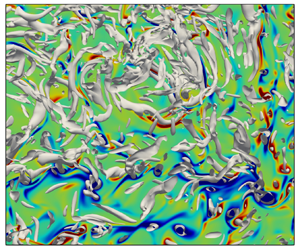
Further insights into the distribution of scales can be gained from figure 12, where we show instantaneous streamwise velocity fluctuations  $u'$ in wall-parallel ( $x$–
$x$– $z$) planes at different wall-normal locations for $Re_\tau =2000$. The $u'$ close to the wall exhibits the organisation of the streaks with a streamwise length of approximately $1000$ and spanwise spacing of $100$. Consistent with the previous findings (Hutchins & Marusic Reference Hutchins and Marusic2007; Bernardini et al. Reference Bernardini, Pirozzoli and Orlandi2014), the outer layer flow exhibits very long regions of positive/negative $u'$. Similar to the finding from energy spectra (figure 9), these streamwise meandering streaks have characteristic lengths $\lambda _z \approx h$ in the spanwise directions. These streaks can be interpreted in terms of large-scale structures that in the form of streamwise vortices of diameters comparable to the channel height (Tamburrino & Gulliver Reference Tamburrino and Gulliver1999; Duan et al. Reference Duan, Chen, Li and Zhong2020) or spatial clusters of hairpin vortices (Kim & Adrian Reference Kim and Adrian1999). In addition, these structures have their footprint both near the wall and the free surface.

Figure 12. Instantaneous streamwise velocity fluctuations ( $u'/u_\tau$) for $Re_\tau =2000$ in $x$–
$x$– $z$ planes at (a) $y^+= 15$, (b) $y^+=384$ ( $y/h=0.19$), (c) $y/h=0.5$ and (d) $y/h=1$. The inset in (a) shows an enlarged view of a box with $2000 \times 1000$ in wall units.
Compared with the CCFs (Bernardini et al. Reference Bernardini, Pirozzoli and Orlandi2014), more small scales are observed at  $y/h=1$ in OCFs (figure 12d). This can be further confirmed by showing the instantaneous wall-normal vorticity $\omega _y$ on the free surface for $Re_\tau =2000$ (figure 13a). Numerous small-scale $\omega _y$ patches (with both positive and negative signs) are observed. Figures 13(b) and 13(c) further show the vortical structures (visualised using the $\lambda _2$ criterion) near the free surface in regions I and II of figure 13(a). Compared with CCFs, more small-scale $\lambda _2$ structures are observed, mainly due to a stronger boundary layer effect near the free surface (Wang et al. Reference Wang, Zhong, Wang and Li2017). As expected, among these structures, some are aligned along the wall-normal direction, which might be generated due to the Kelvin–Helmholtz instability of the free-surface vortex sheet. There also exists significant amounts of $\lambda _2$ vortices that are parallel to the wall. Furthermore, different from the near-wall vortices, which are predominantly aligned along the streamwise direction, the wall-parallel vortices near the free surface have relatively larger tilting angle with respect to the streamwise direction. Interestingly, some of these vortices are even oriented along the spanwise direction, which is consistent with the recent finding by Duan et al. (Reference Duan, Zhong, Wang, Chen, Wang and Li2021a) that higher relative population density of spanwise vortices occurs in OCFs than in CCFs. Based on the ‘bottom-up’ perspective for the origin of VLSMs, in which VLSMs are viewed as the result of coherence in the pattern of vortices produced near the boundary (Kim & Adrian Reference Kim and Adrian1999), these additional vortical structures near the free surface may be one possible explanation for the increased VLSMs in OCFs: a topic that merits further study.

Figure 13. (a) Instantaneous wall-normal vorticity  $\omega _y$ (normalised by its r.m.s. value) on the free surface for $Re_\tau =2000$ and enlarged view of (b) box I and (c) box II along with the vortical structures visualised using the $\lambda _2$ criterion within $\Delta y^+\le 200$ from the free surface.
3.2.2. Premultiplied spectra of Reynolds shear stress
To investigate the contribution of VLSMs to the Reynolds shear stress and also to the mean wall shear stress, premultiplied cospectra of streamwise and wall-normal velocities are examined here. Figures 14 and 15, respectively, show the premultiplied cospectra  $k_x\varPhi_{uv}/u^2_\tau$ and $k_z\varPhi_{uv}/u^2_\tau$ for different Reynolds numbers in wall units. Similar to the streamwise velocity spectra $k\varPhi_{uu}$ (figures 8 and 9), an inner peak is observed, which is associated with the near-wall coherent structures. The peak occurs at a higher $y^+$ when compared with $k\varPhi_{uu}$. As $Re_\tau$ increases, the energy content in the outer region continues to increase, and a second peak located at $\lambda _z=h$ starts to occur at $Re_\tau =2000$ for the $k_z\varPhi_{uv}/u^2_\tau$ (similar to $k_z\varPhi_{uu}/u^2_\tau$ in figure 10e), but not for $k_x\varPhi_{uv}/u^2_\tau$ (again due to limited streamwise domain size).

Figure 14. Premultiplied cospectra of streamwise and wall-normal velocities  $k_x\varPhi_{uv}/u^2_\tau$ as a function of $\lambda ^+_x$ and $y^+$ for: (a) $Re_\tau =180$, (b) $Re_\tau =550$, (c) $Re_\tau =1000$ and (d) $Re_\tau =2000$.

Figure 15. Premultiplied cospectra of streamwise and wall-normal velocities  $k_z\varPhi_{uv}/u^2_\tau$ as a function of $\lambda ^+_z$ and $y^+$ for: (a) $Re_\tau =180$, (b) $Re_\tau =550$, (c) $Re_\tau =1000$ and (d) $Re_\tau =2000$.
Figure 16 compares the one-dimensional premultiplied cospectra of streamwise and wall-normal velocities  $k_x\varPhi_{uv}$ and $k_z\varPhi_{uu}$ at different $y$ locations for $Re_\tau =2000$. Again, good collapse can be observed between OCF and CCF in the near-wall region (e.g. at $y^+=15$). In the overlap region, both $k_x\varPhi_{uv}$ and $k_z\varPhi_{uv}$ are slightly smaller in OCF than in CCF at small wavelengths, but the trend reverses at large wavelengths, akin to those observed for the streamwise velocity spectra. Interestingly, very close to the free surface (e.g. at $y/h=0.9$), both $k_x\varPhi_{uv}$ and $k_z\varPhi_{uv}$ become larger again in OCFs at small $\lambda _x$ and $\lambda _z$, confirming the prominence of small-scale structures due to the boundary layer effect of the free surface (figure 13). This is also consistent with the finding by Wang et al. (Reference Wang, Zhong, Wang and Li2017), who showed that the free surface restrains the characteristic scales of the streaks and the associated vortical structures. Following (3.3), figures 17(a) and 17(b) show the fraction of Reynolds shear stress carried by VLSMs: $\gamma _{uv}(\lambda _x=3h)$ and $\gamma _{uv}(\lambda _z=0.5h)$. Both of them increase with $y$ and reach approximately $0.5$– $0.6$ at $y/h=0.5$ and then decrease near the free surface, particularly for the spanwise case. Again, at a given $Re_\tau$, the maximum values are slightly larger than that for CCF, highlighting the free surface effect in OCFs.

Figure 16. Premultiplied cospectra of streamwise and wall-normal velocities (a)  $k_x\varPhi_{uv}$ and (b) $k_z\varPhi_{uv}$ at different $y$ locations for $Re_\tau =2000$. The solid and dashed lines represent OCF and CCF, respectively.


3.3. Scale contribution to the skin friction
In this section, we further investigate the contributions of different scale motions to the mean wall shear stress (or, equivalently, the skin friction) and compare the difference between OCFs and CCFs. Based on the Fukagata–Iwamoto–Kasagi (FIK) identity (Fukagata, Iwamoto & Kasagi Reference Fukagata, Iwamoto and Kasagi2002), the skin friction coefficient can be directly linked to the alteration of the Reynolds shear stress:
 \begin{equation} C_f=\underbrace{\frac{6}{Re_b}}_{C^L_f}+\underbrace{\frac{6}{U^2_b}\int^1_0(1-y)(-\left\langle{u'v'}\right\rangle)\,{{\rm d} y}}_{C^T_f}, \end{equation}
which has been obtained for OCF by Duan et al. (Reference Duan, Zhong, Wang, Zhang and Li2021b). The skin friction coefficient  $C_f\equiv 2\tau _w/(\rho U^2_b)$ thus has an ‘equivalent’ laminar part $C^L_f$, and a turbulent part $C^T_f$ represented by the weighted integration of the total Reynolds shear stress. Table 3 lists the estimated skin friction using (3.4) at different Reynolds numbers. Note that for all cases, the relative error of $C_f$ between the direct calculation based on the definition and the FIK identity is within $\pm$1 %. In addition, at the same Reynolds number, $C_f$ and its laminar and turbulent components are identical between OCFs and CCFs. As expected, the turbulent contribution becomes larger as $Re_\tau$ increases, changing from approximately $74\,\%$ at $Re_\tau = 200$ to $97\,\%$ at $Re_\tau = 2000$.
Table 3. The skin friction coefficient and its decomposition based on FIK identity.
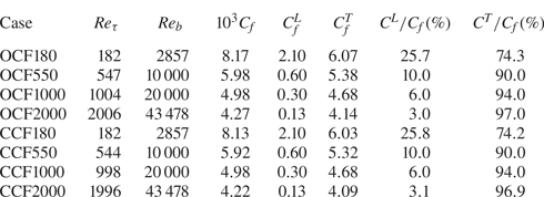
To further quantify the contributions to  $C_f$ from different scales, the FIK identity in combination with the wavenumber spectra of the Reynolds shear stress (Deck et al. Reference Deck, Renard, Laraufie and Weiss2014; Yao, Chen & Hussain Reference Yao, Chen and Hussain2019) is employed. The total Reynolds shear stress can be expressed in terms of one-dimensional Reynolds shear stress spectral density, i.e.
 \begin{equation} -\left\langle{u'v'}\right\rangle(y)=\int^\infty_{-\infty}\varPhi_{uv}(y;k) \,\mathrm{d} k. \end{equation}
Therefore, (3.4) can be further expressed as
 \begin{align} C_{f} &=\frac{6}{Re_b}+\frac{6}{U^2_b}\int^1_0\int^\infty_{-\infty} (1-y)\varPhi_{uv}(y;k) \,\mathrm{d}k \,\mathrm{d} y, \end{align}
 \begin{align} &=\frac{6}{Re_b}+\int^\infty_{-\infty} \underbrace{\int^1_0 \frac{6}{U^2_b}(1-y)\varPhi_{uv}(y;k) \,\mathrm{d} y}_{\varPhi_{T}}\,\mathrm{d}k. \end{align}
Then, the contribution of a specific length scale to  $C_f$ can be represented by $\varPhi _{T}(k)$.
Figure 18(a,b) shows the  $k_x\varPhi _{T}/C_f$ and $k_z\varPhi _{T}/C_f$ as a function of $\lambda _x$ and $\lambda _z$, respectively. Note that the total area below curve $k_x\varPhi _{T}/C_f$ and $k_z\varPhi _{T}/C_f$ equals the total ‘turbulent’ contribution to $C_f$. Except for the OCF180 case, $k_x\varPhi _{T}/C_f$ peaks at $\lambda _x=1\sim 2h$, consistent with the observation by Duan et al. (Reference Duan, Zhong, Wang, Zhang and Li2021b). In addition, for the OCF2000 case, a second peak develops around $\lambda _x=10h$, which corresponds to the contribution from VLSMs. For $k_z\varPhi _{T}/C_f$, the location of the peak shifts towards larger $\lambda _z$ with increasing $Re_\tau$ and becomes $\lambda _z=1h$ for $Re_\tau =2000$, which is due to the dominant role of VLSMs to the Reynolds shear stress at high $Re_\tau$. Although the shape is similar between OCF and CCF, notable differences can be observed. In the wavelength range of $\lambda _x<10h$(or $\lambda _z< h$), the $k_x\varPhi _f/C_f$ ( $k_z\varPhi _f/C_f$) in OCF is smaller than that in CCF. However, the trend reverses for $\lambda _x>10h$ ( $\lambda _z>1h$), suggesting a high contribution to $C_f$ for turbulent motions at very large length scales in OCFs.

Figure 18. Comparison of (a)  $k_x\varPhi _{T}/C_f$ and (b) $k_z\varPhi _{T}/C_f$ between OCF (solid) and CCF (dashed) cases. For better display, the curves are vertically shift by $0.1$ and $0.2$ in (a,b), respectively.
Due to limited streamwise domain size,  $k_x\varPhi _{T}/C_f$ still remains relatively large at the largest $\lambda _x$ considered, whereas $k_z\varPhi _{T}/C_f$ decays to zero at large $\lambda _z$, suggesting the adequacy of the spanwise domain size. In the following, we further employ $k_z\varPhi _{T}/C_f$ to determine the contribution to skin friction from a range of scales. The cumulative turbulent contribution is defined as
 \begin{equation} Cum_T(\lambda_z)=\int^\infty_{2{\rm \pi}/\lambda_z} k_z\varPhi_{T}/C_f \,\mathrm{d} k_z, \end{equation}
which represents the total turbulent contributions for all spanwise scales smaller than a given wavelength  $\lambda _z$. By choosing appropriate cut-off wavelength ranges, the contribution from the specified scale range can be obtained. For example, figure 19(a) shows the fractions contributed by different scales when choosing the typical cut-off wavelength $\lambda _z=0.5h$ to separate LSMs and VLSMs. With this threshold, there is a negligible difference between OCFs and CCFs. Although the laminar contribution to $C_f$ decreases with increasing $Re_\tau$, the contribution from turbulent motions with wavelength $\lambda _z<0.5h$ increases continuously, becoming approximately $44\,\%$ at $Re_\tau =2000$. In addition, for all cases, the VLSMs (with a spanwise wavelength $\lambda _z>0.5h$) contribute more than 50 %. Further results are obtained by using a larger dividing wavelength of $\lambda _z=1h$ (figure 19b). The contribution to $C_f$ from turbulent motions with $\lambda _z>1h$ continuously increases with $Re_\tau$. It becomes approximately 30 % at $Re_\tau =2000$ in OCFs, slightly higher than that in CCFs, which is consistent with the observation in figure 18. Most importantly, the discrepancy between OCFs and CCFs seems to enlarge with $Re_\tau$, suggesting that at very high Reynolds numbers, the contribution from VLSMs to the Reynolds shear stress and also to skin friction would be quite different.

Figure 19. Contributions of different scales to the skin friction by using the cut-off wavelength (a)  $\lambda _z=0.5h$ and (b) $\lambda _z=1h$.
Note that the above analysis based on the FIK analysis and spectra decomposition have certain caveats. For example, there is a lack of physical interpretation for the linear weight of Reynolds shear stress in (3.4). To overcome this issue, many other skin friction decomposition methods have been proposed (e.g. Renard & Deck Reference Renard and Deck2016; Chen, Yao & Hussain Reference Chen, Yao and Hussain2021). In addition, we assume that the turbulent motions of a particular scale can be fully represented by a specific Fourier mode. This might not reflect the true flow physics in wall turbulence considering the modulation effects may spread over a wide range of Fourier modes (Ganapathisubramani et al. Reference Ganapathisubramani, Hutchins, Monty, Chung and Marusic2012).
4. Conclusions
DNS of turbulent OCF for friction Reynolds number  $Re_\tau$ up to $2000$ have been presented. Various flow statistics are collected and compared with the CCFs. As expected, the mean velocity profiles between OCFs and CCFs collapse in the near-wall region but differ in the outer region. In particular, due to the presence of the free surface, the wake region is smaller in OCFs. In addition, different from CCFs, a distinct log layer with Kárman constant $\kappa =0.363$ is observed for OCF at $Re_\tau =2000$, whereas the range is further away from the wall (i.e. $y/h$ from 0.25 to 0.6) compared with the usual log layer. Except for a very thin layer near the free surface, the Reynolds stresses and vorticity fluctuations agree well between OCFs and CCFs. The Reynolds number scaling of the near-wall averaged quantities, particularly the vorticity variances at the wall, seem to follow closely the defect power law proposed by Chen & Sreenivasan (Reference Chen and Sreenivasan2021, Reference Chen and Sreenivasan2022).
Contributions of different scales to the turbulence statistics are quantified based on the energy spectra. The very-large-scale structures (with streamwise wavelength  $\lambda _x>3h$ or spanwise wavelength $\lambda _z>0.5h$) are shown to make a significant contribution to turbulence statistics, with over 60 % of streamwise turbulence intensity and Reynolds shear stress in the overlap and outer layers. In addition, these structures maintain higher strength in the outer layer when compared with the CCFs, suggesting that the free surface can sustain/promote VLSMs. The higher strength of VLSMs is also the main reason for the higher streamwise turbulence intensity in the outer region. Flow visualisations reveal that more small-scale structures are generated near the free surface, presumably due to its boundary layer effect. According to the ‘bottom-up’ perspective of the VLSMs’ origin, these structures might be one of the main reasons for the enhanced VLSMs in OCFs. Further studies are still required to better explain how the free surface affects the VLSMs. Finally, the contribution to the mean wall shear stress from scales with $\lambda _z > h$ increases with Reynolds number and becomes approximately 30 % at $Re_\tau =2000$, slightly higher than the CCFs at the same $Re_\tau$. As a conclusion, the presence of the free surface in OCFs has significant effects on flow dynamics, such as the development of the log layer in the mean velocity profile at lower $Re_\tau$, redistribution of turbulent kinetic energy and the enhancement of VLSMs.
Acknowledgements
We appreciate M. Lee and R. Moser for providing us with their channel flow code, which is used for this study. We are also grateful to Q. Zhong for providing the experimental data. Computational resources provided by Texas Tech University HPCC, TACC Lonestar, Stampede2 and Frontera are acknowledged.
Funding
J.Y. and F.H. are funded by TTU Distinguished Chair. X.C. acknowledges support from the National Natural Science Foundation of China, grant numbers 12072012, 11721202 and 91952302, and “the Fundamental Research Funds for the Central Universities”.
Declaration of interests
The authors report no conflict of interest.
Data availability statement
The data that support the findings of this study are openly available in Texas Data Repository at https://dataverse.tdl.org/dataverse/tocf/.
Appendix. Domain size effect in turbulent OCFs
The effect of domain size on flow statistics and structures is further examined here. We first perform additional DNS with various streamwise and spanwise lengths at  $Re_\tau =550$. The details of domain sizes, grid sizes and resolutions are listed in table 4. Figure 20 shows the mean streamwise velocity and Reynolds stress profiles for different domain size cases. The agreement between them is reasonably good across the whole channel, consistent with the findings by Lozano-Durán & Jiménez (Reference Lozano-Durán and Jiménez2014) for the CCFs. Figures 21(a) and 21(b) further shows the premultiplied streamwise and spanwise spectra of the streamwise velocity fluctuations $k_x\varPhi_{uu}/u^2_\tau$ and $k_z\varPhi_{uu}/u^2_\tau$ for different domain size cases. The spectrum of $k_x\varPhi_{uu}/u^2_\tau$ is truncated by the box, particularly for the shorter streamwise domain size cases. However, for all cases, the contours collapse at small wavelengths and differ at large ones. Even for this large streamwise domain, the lowest contour ( $k_x\varPhi_{uu}/u^2_\tau =0.2$) is not closed. For the largest streamwise domain size case (i.e. OCF550SL), a second peak located at $\lambda ^+_x=10{\,}000$ (or $\lambda _x/h\approx 18$) develops in the outer region. The $k_z\varPhi_{uu}/u^2_\tau$ spectrum is closed for all cases, indicating $L_z=2{\rm \pi}$ is wide enough to capture most energy of the streamwise velocity fluctuations. Although the contours collapse at small $\lambda ^+_z$, they differ at larger $\lambda ^+_z$, particularly near the free surface. This suggests that the spanwise domain size has a notable effect on the distributions of energy and Reynolds stress, particularly at large scales.
Table 4. Details of the numerical discretisation employed for the OCF simulations. The computational box size is  $L_x \times L_y \times L_z$, with $h$ the channel height; and $N_x$, $N_y$ and $N_z$ are the number of grid sizes in each direction. Here $T u_\tau /h$ is the total simulation time without transition.


Figure 20. (a) Mean velocity and (b) Reynolds stress as a function of  $y^+$ for different domain size effect at $Re_\tau=550$.

Figure 21. Premultiplied streamwise and spanwise spectra of the streamwise velocity fluctuations (a)  $k_x\varPhi_{uu}/u^2_\tau$ and (b) $k_z\varPhi_{uu}/u^2_\tau$ for different domain sizes at $Re_\tau =550$.
Finally, an additional case (i.e. OCF2000SL) with double the streamwise domain size but half the spanwise domain size as OCF2000 is considered. Figure 22 compares the premultiplied streamwise and spanwise spectra of the streamwise velocity fluctuations  $k_x\varPhi_{uu}/u^2_\tau$ and $k_z\varPhi_{uu}/u^2_\tau$ in outer units. Again, the contours collapse at small wavelengths for both cases. The $k_x\varPhi_{uu}/u^2_\tau$ spectrum is truncated by the box for OCF2000 case. However, for the OCF2000SL case, although the lowest contour ( $k_x\varPhi_{uu}/u^2_\tau =0.2$) is not closed, a distinct outer peak develops with streamwise wavelength $\lambda _x/h=4{\rm \pi}$, larger than that observed by Lee & Moser (Reference Lee and Moser2015) for CCF at $Re_\tau =2000$. The spectrum of $k_z\varPhi_{uu}/u^2_\tau$ has a similar shape as that at $Re_\tau =550$, but the outer peak located at $\lambda _z/h\approx 2{\rm \pi} /5$ is much stronger.

Figure 22. Premultiplied streamwise and spanwise spectra of the streamwise velocity fluctuations (a)  $k_x\varPhi_{uu}/u^2_\tau$ and (b) $k_z\varPhi_{uu}/u^2_\tau$ for two different domain size cases at $Re_\tau =2000$.


 Open access