


1. Introduction
Searching for nonlinear travelling waves in an inviscid fluid layer is a research field with a long history in the water-wave community dating back to Stokes. It is well known that the limiting configuration of surface gravity waves, i.e. the Stokes highest wave, features a stagnation-point singularity at its crest with a local  $120^{\circ }$ angle. For capillary waves, Crapper (Reference Crapper1957) and Kinnersley (Reference Kinnersley1976) found exact analytical solutions in water of infinite and finite depths, respectively. Their large-amplitude solutions demonstrate an overhanging U-shaped structure. The profile is considered to reach a limiting configuration as the free surface develops a point of contact with a ‘trapped bubble’ at the trough (see figure 1a).

Figure 1. Three limiting configurations: (a) type I, (b) type II, and (c) type III.
The limiting profiles of free-surface progressive gravity water waves were later generalized to interfacial waves between two immiscible fluids of constant densities. The limiting configuration of periodic interfacial gravity waves has been studied for decades (Meiron & Saffman Reference Meiron and Saffman1983; Turner & Vanden-Broeck Reference Turner and Vanden-Broeck1986). It is found that the interface can also develop an overhanging profile tending to be self-intersecting. Grimshaw & Pullin (Reference Grimshaw and Pullin1986) proposed a possible limiting configuration that features a closed bubble of heavier fluid on top of a  $120^{\circ }$ angle crest. However, the exact limiting profiles are numerically challenging due to the local stagnation-point singularity. Recently, Maklakov & Sharipov (Reference Maklakov and Sharipov2018), Guan et al. (Reference Guan, Vanden-Broeck, Wang and Dias2021a) and Guan, Vanden-Broeck & Wang (Reference Guan, Vanden-Broeck and Wang2021b) extended the previous works and provided solid numerical evidence for the existence of such limiting solutions. In particular, Guan et al. (Reference Guan, Vanden-Broeck and Wang2021b) confirmed that there are actually three types of limiting configurations, which can coexist and are linked via a secondary bifurcation point when the relevant parameters are well chosen. Therefore, it is interesting to see if an analogous bifurcation mechanism and new solutions can be obtained for purely capillary interfacial waves, in which gravity is neglected.
Based on a hodograph transformation, Crapper (Reference Crapper1957) first found a family of exact travelling-wave solutions for pure capillary waves on a fluid of infinite depth, whose uniqueness was established by Okamoto & Shoji (Reference Okamoto and Shoji1991) and Okamoto (Reference Okamoto2005) under a certain positivity assumption. Crapper's pioneering work was later extended by various investigators. Kinnersley (Reference Kinnersley1976) generalized Crapper waves to the case of finite depth and obtained exact nonlinear solutions involving elliptic functions. Crowdy (Reference Crowdy2000) provided a different derivation of Crapper waves using conformal maps. Blyth & Vanden-Broeck (Reference Blyth and Vanden-Broeck2004) considered capillary waves on fluid sheets with two free surfaces and found secondary bifurcation branches on the symmetric Kinnersley's solution branch. Akers, Ambrose & Wright (Reference Akers, Ambrose and Wright2013) computed progressive capillary waves between two semi-infinite fluids of equal density in the presence of background shear currents. Akers, Ambrose & Wright (Reference Akers, Ambrose and Wright2014) perturbed Crapper waves by gravity to show the existence of overhanging solutions for capillary–gravity waves. The stability properties of capillary waves were investigated by Tiron & Choi (Reference Tiron and Choi2012) for Crapper waves and by Blyth & Părău (Reference Blyth and Părău2016) for fluid sheets.
In the present paper, progressive interfacial capillary waves between two immiscible fluids in a channel are studied numerically via a Cauchy-type boundary integral formulation (see § 2). Using the Fourier series method, we obtain in § 3 highly accurate numerical solutions and bifurcations in various cases. New solutions are found to bifurcate from the branches that arise from infinitesimal periodic waves (referred to as the primary branches hereafter) for special sets of parameters (for example, when both layers are of the same density and thickness), akin to the bifurcation mechanism found by Guan et al. (Reference Guan, Vanden-Broeck and Wang2021b) for interfacial gravity waves. When the parameters are perturbed, these new branches separate from the primary ones and become isolated curves. Besides the limiting waves of the self-intersecting type, we also find two other limiting solutions of boundary-touching type: see figure 1(b) for one-wall touch, and figure 1(c) for simultaneous two-wall touch. For convenience, the limiting configurations shown in figures 1(a–c) are termed type I, type II and type III limits, respectively. In § 4, we examine the geometric characteristics of the boundary-touching interfaces, which are shown to be piecewise circular. This fact enables us to predict the types of limiting waves for most parameter settings.
2. Boundary integral formulation
Consider two-dimensional progressive waves of wavelength  $\lambda$ and speed $c$ through the interface between two incompressible, inviscid and immiscible fluids (see the sketch in figure 2). We choose a moving frame of reference in which the waves are steady. We denote by $h_j$ and $\rho _j$ ( $\kern0.06em j=1,2$) the mean depths and densities in each fluid layer, where subscripts 1 and 2 refer to fluid properties associated with the lower and upper fluid layers, respectively. A Cartesian coordinate system is introduced such that the $x$-axis is on the mean level of the interface, and the $y$-axis coincides with a line through a wave crest/trough. It is convenient to choose $\lambda /(2{\rm \pi} )$ and $c$ as the units of length and velocity. In addition, the only restoring force under consideration is surface tension, and we confine ourselves to solutions with mirror symmetry about the $y$-axis. The flows are supposed to be irrotational; hence there exist potential functions $\phi _1$ and $\phi _2$ satisfying the Laplace equation in the respective domains, namely,
 $$\begin{gather} \phi_{1,xx}+\phi_{1,yy}=0,\quad\text{for}\ {-h_1}< y<\eta(x), \end{gather}$$
 $$\begin{gather}\phi_{2,xx}+\phi_{2,yy}=0,\quad\text{for}\ \eta(x)< y< h_2, \end{gather}$$
where  $\eta (x)$ stands for the displacement of the interface. We denote by $w_j(z)=\phi _{j,x}-\mathrm {i}\,\phi _{j,y}$ the complex velocity in the corresponding fluid layer ( $\kern0.06em j=1,2$), where $z=x+\mathrm {i}y$. Applying the Schwarz reflection principle to the lower and upper layers, the flow domains become
 $$\begin{gather} S_1=[-{\rm \pi}, {\rm \pi}]\times[{-}2h_1-\eta, \eta], \end{gather}$$
 $$\begin{gather}S_2=[-{\rm \pi}, {\rm \pi}]\times[\eta, 2h_2-\eta ], \end{gather}$$
and the complex velocities remain analytical functions in the extended regions. It then follows from the Cauchy integral formula that
 \begin{equation} w_j(z_0) = \frac{1}{\mathrm i {\rm \pi}}\oint_{\partial S_j} \frac{w_j(z)}{z-z_0}\,\mathrm{d}z, \end{equation}
where  $\partial S_j$ represents the boundary of the region $S_j$, $z_0$ denotes a point on $\partial S_j$, and the integral is in the Cauchy principal sense. Note that the integral requires only the information on the interface owing to the Schwarz reflection principle, which significantly reduces the number of unknowns. Following Papageorgiou & Vanden-Broeck (Reference Papageorgiou and Vanden-Broeck2004), we introduce a variable transformation
 \begin{equation} \zeta = \mathrm{e}^{-\mathrm{i} z}, \end{equation}
which maps  $S_j$ onto an annular region in the $\zeta$-plane. Note that we can express the complex velocity $w_j$ in terms of the velocity modulus $q_j$ and the inclination angle $\gamma$ as
 \begin{equation} w_j=q_j\,\mathrm{e}^{-\mathrm{i}\gamma}. \end{equation}
On the interface,  $\gamma$ is defined by
 \begin{equation} \gamma ={-}\mathrm{i}\ln (\mathrm{d}z/\mathrm{d}s), \end{equation}
where  $s$ is the arc length parameter in the physical space. Without loss of generality, we will let $s = 0$ be the intersection point of the interface and the $y$-axis, corresponding to a wave crest or trough due to symmetry. Using the Cauchy integral formula and assumed symmetry property of waves, we obtain two integral equations for the lower and upper layers, respectively:
 \begin{align} &{\rm \pi}\, q_1(\sigma)\,x'(\sigma)\nonumber\\ &\quad ={-}\int_{0}^\alpha\left(\frac{q_1(s)\,(1-\mathrm{e}^{Y_+{+}2h_1}\cos(X_-))}{1+\mathrm{e}^{2(Y_+{+}2h_1)}-2\mathrm{e}^{Y_+{+} 2h_1}\cos(X_-)}-\frac{q_1(s)\,(1-\mathrm{e}^{Y_-}\cos(X_-))}{1+\mathrm{e}^{2Y_-}-2\mathrm{ e}^{Y_-}\cos(X_-)}\right)\mathrm{d}s\nonumber\\ &\qquad -\int_{0}^\alpha\left(\frac{q_1(s)\,(1-\mathrm{ e}^{Y_+{+}2h_1}\cos(X_+))}{1+\mathrm{e}^{2(Y_+{+}2h_1)}-2\mathrm{ e}^{Y_+{+}2h_1}\cos(X_+)}-\frac{q_1(s)\,(1-\mathrm{e}^{Y_-}\cos(X_+))}{1+\mathrm{ e}^{2Y_-}-2\mathrm{e}^{Y_-}\cos(X_+)}\right)\mathrm{d}s, \end{align}
 \begin{align} &{\rm \pi}\,q_2(\sigma)\,x'(\sigma)\nonumber\\ &\quad ={-}\int_{0}^\alpha\left(\frac{q_2(s)\,(1-\mathrm{ e}^{Y_-}\cos(X_-))}{1+\mathrm{e}^{2Y_-}-2\mathrm{ e}^{Y_-}\cos(X_-)}-\frac{q_2(s)\,(1-\mathrm{e}^{Y_+{-}2h_2}\cos(X_-))}{1+\mathrm{ e}^{2(Y_+{-}2h_2)}-2\mathrm{e}^{Y_+{-}2h_2}\cos(X_-)}\right)\mathrm{d}s\nonumber\\ &\qquad-\int_{0}^\alpha\left(\frac{q_2(s)\,(1-\mathrm{ e}^{Y_-}\cos(X_+))}{1+\mathrm{e}^{2Y_-}-2\mathrm{ e}^{Y_-}\cos(X_+)}-\frac{q_2(s)\,(1-\mathrm{e}^{Y_+{-}2h_2}\cos(X_+))}{1+\mathrm{ e}^{2(Y_+{-}2h_2)}-2\mathrm{e}^{Y_+{-}2h_2}\cos(X_+)}\right)\mathrm {d}s, \end{align}
where  $Y_+ = \eta (\sigma )+\eta (s)$, $Y_- = \eta (\sigma )-\eta (s)$, $X_+=x(\sigma )+x(s)$ and $X_- = x(\sigma )-x(s)$. Here, $\sigma \in [0,\alpha ]$ is the arc length parameter of the interface, where $\alpha$ is the total arc length of the interfacial wave in half period, and the prime notation represents derivative with respect to arc length. To close the system, we need the Bernoulli equation
 \begin{equation} R q_2^2-q_1^2+ 2\kappa/\mu = B,\end{equation}
and the arc length equation
 \begin{equation} x'(s)^2+\eta'(s)^2 = 1,\end{equation}
where  $R= \rho _2/\rho _1$ is the density ratio, $\kappa =x'(s)\,\eta ''(s)-x''(s)\,\eta '(s)$ is the curvature, $B$ is the unknown Bernoulli constant, and $\mu = \rho _1 \lambda c^2/(2{\rm \pi} T)$, with $T$ being the surface tension coefficient. The density ratio $R=0$ corresponds to the free-surface capillary waves. Note that one can fix $B = R-1$ or other constants, which amounts to different definitions of wave speed and background current (Vasan & Deconinck Reference Vasan and Deconinck2013). For solitary waves or periodic deep-water waves, there is a particular frame of reference where the velocity at infinity is zero; thus it is a convenient choice for mathematical formulation. However, there is no preference among all inertial references for periodic waves on water of finite depth. These waves travel at different speeds in different frames of reference, thus having distinct Bernoulli constants. Fixing $B = R-1$ means choosing a specific frame of reference where periodic waves bifurcate from a uniform flow, and defining wave speed so that $B$ is invariant along the whole bifurcation branch. However, in the subsequent calculations, we treat $B$ as a fundamental unknown and apply the following definition of wave speed:
 \begin{equation} 1 ={-}\frac{1}{2{\rm \pi}}\int_{-{\rm \pi}}^{\rm \pi} u_1\,{{\rm d} x} ={-}\frac{1}{2{\rm \pi}}\int_{-{\rm \pi}}^{\rm \pi} u_2\,{{\rm d}x},\end{equation}
where the negative sign is chosen so that the background current is from right to left in the moving frame of reference.

Figure 2. Schematic of one wavelength of the waves.
3. Numerical method and results
3.1. Fourier method
Following Guan et al. (Reference Guan, Vanden-Broeck and Wang2021b), we introduce a normalized arc length  $\tau = s/\alpha \in [0,1]$ and write the unknowns $q_1$, $q_2$, $x$ and $\eta$ as the following Fourier series:
 $$\begin{gather} q_1(\tau)=\sum_{n=0}^{\infty}a_n\cos(n{\rm \pi} \tau),\quad q_2(\tau)=\sum_{n=0}^{\infty}b_n\cos(n{\rm \pi} \tau), \end{gather}$$
 $$\begin{gather}x(\tau)=c_0\tau+\sum_{n=1}^{\infty}\frac{c_n}{n{\rm \pi}}\sin(n{\rm \pi} \tau),\quad\eta(\tau)=d_0-\sum_{n=1}^{\infty}\frac{d_n}{n{\rm \pi}}\cos(n{\rm \pi} \tau). \end{gather}$$
Truncating these series after  $N$ terms gives $4N$ unknowns: $a_j$, $b_j$, $c_j$ and $d_j$ (for $j=0,1,\ldots,N-1$). However, the periodicity condition, $x(1)-x(0) = {\rm \pi}/2$, immediately gives $c_0 = {\rm \pi}/2$. Therefore, together with $\alpha$, $\mu$ and $B$, there are $4N+2$ unknowns in total to be found. We introduce $N$ equally spaced collocation points
 \begin{equation} \tau_j = \frac{j-1}{N-1}, \quad j=1,2,\ldots,N, \end{equation}
at which (2.9)–(2.13) are satisfied. To avoid singularities in the Cauchy integral, we introduce another set of mesh points
 \begin{equation} \tau_j^m = \frac{\tau_j+\tau_{j+1}}{2},\quad j = 1,2,\ldots,N-1, \end{equation}
and evaluate the integrals by applying the midpoint rule. The values of unknowns on the midpoint  $\tau _j^m$ are calculated using (3.1a,b) and (3.2a,b). Note that there are two more conditions,
 $$\begin{gather} \int_0^{\rm \pi} \eta(x)\,{{\rm d} x} = 0, \end{gather}$$
 $$\begin{gather}\int_0^{\rm \pi} \eta'(x)\,{{\rm d} x} ={-}H, \end{gather}$$
representing the zero-mean interface and the pre-assigned wave amplitude. A closed algebraic system with  $4N+2$ unknowns and $4N+2$ equations can be obtained if we abandon two integral equations, for example, those evaluated at $\tau = 1$ (Guan et al. Reference Guan, Vanden-Broeck and Wang2021b). However, in the present work, we select one evaluated at $\tau = 1$ in (2.9), and the other evaluated at $\tau =0$ in (2.10). It turns out that this numerical scheme, together with the Newton iteration method, gives very accurate results. The iteration process terminates when the maximum residual of the system is less than $10^{-10}$. At the same time, we monitor the residuals of the two abandoned integral equations (denoted by $\delta$), which we require to be less than $10^{-4}$ for an appropriate choice of $N$. Generally, we start calculating with $N=300$; the value of $\delta$ is of $O(10^{-10})$ for most numerical solutions. So these two abandoned integral equations are satisfied numerically. When the local curvature increases drastically, we increase $N$ to ensure that $\delta <10^{-4}$. All the numerical results presented were recalculated with a larger $N$ to ensure that they are grid-independent within graphical accuracy.
3.2. Numerical results
We do not need to worry about the Rayleigh–Taylor instability since we neglect gravity. Therefore, all non-negative density ratios are allowed. However, solutions for  $(h_1,h_2,R)$ have a one-to-one relation to solutions for $(h_2,h_1,1/R)$ if one notices that the two-fluid system can be turned upside down, namely by reversing the direction of the $y$-axis. This relation can be established by mapping $(\mu,B)$ to $(R\mu,-B/R)$ in the Bernoulli equation. Therefore, we will focus on only $R\in [0,1]$ in the subsequent computations.
In the first example, we set  $h_1=h_2=100$ to approximate the deep-water limit and calculate solutions for different values of $R$. In figure 3(a), we plot a collection of speed–amplitude bifurcation curves, starting with infinitesimal periodic waves. The linear dispersion relation is $\mu \approx 1/(1+R)$ in this situation. In figure 3(b), the same branches are plotted in the $(B,|H|)$-plane. On each branch, the Bernoulli constant is $B = R-1$. This is valid under the deep-water assumption. For each value of $R$, as the wave amplitude increases, the wave profile gradually overhangs and ultimately develops a point of contact enclosing a pendant-shaped bubble (i.e. the type I limit). These extreme waves are labelled by the circles in figures 3(a) and 3(b). For the particular case $R=0$, the solutions are the well-known Crapper waves with a limiting wave height $|H|\approx 1.46{\rm \pi}$ (see Crapper (Reference Crapper1957) for the explicit expression). In figures 3(a) and 3(c), the theoretical results of the Crapper waves (black dots) are compared with our numerical solutions. The amplitude of the limiting wave increases as the density ratio increases; therefore the numerical calculation becomes more difficult for larger $R$. Typical profiles are shown in figure 3(d) for various $R$. The numerical accuracy is shown in table 1 by comparing the values of $\mu$ for $h_1=h_2=100$ and $R=0$ with the exact values of the Crapper waves for given wave amplitudes. Remarkably, our numerical scheme provides at least 9-decimal-places accuracy for most solutions; even for the limiting waves, a 7-decimal-places agreement can be achieved with $N=500$. Both Crapper (Reference Crapper1957) and Kinnersley (Reference Kinnersley1976) chose $B=-1$ in their calculations. This choice is equivalent to our definition of wave speed (2.13) only when the fluid is of finite depth. Therefore, we choose the Crapper wave, rather than the Kinnersley solution, to compare, although the latter deals with the finite-depth situation.

Figure 3. Bifurcation diagrams and limiting profiles for  $h_1=h_2=100$. (a) Speed–amplitude bifurcation curves for various density ratios. The circles correspond to the self-intersecting solutions, and the black dots represent the Crapper waves. (b) Bifurcation curves in the $(B,|H|)$-plane for various density ratios. (c) Limiting profiles for $R=0$: solid line indicates the numerical solution, and dots indicate the analytic solution. (d) Typical limiting profiles for $R=0.1$, 0.3, 0.5, 0.7 and 0.9, from left to right, respectively.
Table 1. Comparison of  $\mu$ between numerical results and Crapper's exact solutions for $h_1=h_2=100$ and $R=0$.

In the second numerical experiment, we let  $h_1=h_2=1$, a shallow-water case. The linear dispersion relation gives $\mu = 1/(\coth (h_1)+\coth (h_2))\approx 0.3808$. We start the computation with small-amplitude sinusoidal waves, and complete this bifurcation curve via a numerical continuation. Besides this primary branch, other bifurcation curves also exist. This is illustrated clearly by considering first the particular case $R=1$. In figure 4(a), we plot the primary and new bifurcation curves (shown by blue and red, respectively) in the $(\mu,|H|)$-plane and $(B,|H|)$-plane. Interestingly, these curves are linked together via secondary bifurcations. The black dot represents the secondary bifurcation point where the new branches start. Note that the left plot has two coinciding red curves. Three typical solutions corresponding to the crosses are plotted in figure 4(b). One can see that the solutions on the primary branch are invariant under the upside-down operation, which yields a zero Bernoulli constant. However, waves on the new branches mirror each other under an upside-down manipulation, thus having Bernoulli constants of opposite signs. We stop the numerical continuation when the wave crest/trough almost touches a wall boundary (shown by $\vartriangle$, $\triangledown$, and
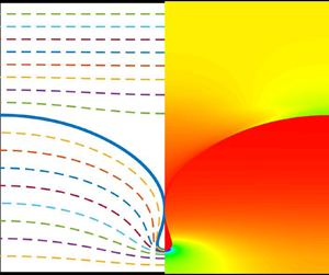
  $\diamond$ in figure 4a), because Newton's method converges poorly if the wave amplitude is increased further. These almost limiting profiles (solid lines), together with the typical streamline pattern (dashed lines) and cloud image of the velocity field, are shown in figure 4(c). Due to small fluid depths, the waves develop the type II and type III limits rather than the type I limit. We then vary the value of the density ratio to understand the bifurcation mechanism for relatively general cases. If the value of $R$ is decreased slightly, then all these branches break up from the secondary bifurcation point, forming separated curves, as shown in figure 4(d). We should point out that a similar bifurcation mechanism was found by Guan et al. (Reference Guan, Vanden-Broeck and Wang2021b) for interfacial gravity waves.

Figure 4. Bifurcation mechanism and almost limiting profiles for  $h_1=h_2 = 1$. (a) Bifurcation curves in the $(\mu,|H|)$-plane and the $(B,|H|)$-plane for $R=1$. The black dot is the secondary bifurcation point where the new branches (red line) grow. The almost limiting profiles denoted by $\vartriangle$, $\triangledown$ and $\diamond$ correspond to top-touching, bottom-touching and top-bottom-touching solutions. (b) Typical wave profiles corresponding to the crosses in (a). (c) Velocity fields of the almost limiting solutions corresponding to $\diamond$ and $\triangledown$ in (a). The solid and dashed curves are interfaces and streamlines, respectively, and velocity magnitudes are shown on the right with different colours. (d) Bifurcation curves in the $(\mu,|H|)$-plane and the $(B,|H|)$-plane for $R=1$ (black), $R=0.99$ (blue), $R=0.95$ (red) and $R=0.8$ (yellow).
If the fluid depths increase to a certain level, then the limiting configuration is expected to become self-intersecting, as in the deep-water case shown in figure 3. In figure 5, we set  $R=1$, and $h_1=h_2=5$ and $h_1=h_2=10$, and the speed–amplitude bifurcation curves are shown in figure 5(a). Similarly, secondary bifurcation points are found on the primary branches (blue), from which new branches appear. Three (almost) limiting configurations for $h_1=h_2=5$ are plotted in figure 5(b). Solutions on the primary bifurcation branch feature an upside-down symmetry and ultimately form a top-bottom-touching singularity labelled by $\diamond$ in figure 5(a). On the new branches, the solutions develop overhanging profiles as the wave amplitude $|H|$ increases, and become self-intersecting before the interface touches the boundary. We plot the streamline pattern and velocity cloud image in figure 5(c) for the type I limit. It is observed that the flow in the upper layer is almost a uniform flow with unit velocity except near the bubble, where it becomes almost stationary. As for the lower layer, the flow is almost static under the wave crest, while the velocity reaches its maximum in a small region under the wave trough. The bifurcation mechanism and limiting configuration for $h_1=h_2=10$ are similar to those for $h_1=h_2=5$.

Figure 5. Bifurcation curves and wave profiles for two sets of parameters:  $R=1$, $h_1=h_2=5$ and $R=1$, $h_1=h_2=10$. (a) Primary bifurcation branches (blue) and new branches (red) are linked by a secondary bifurcation point (black dots). (b,d) Almost limiting profiles for $h_1=h_2=5$ and $h_1=h_2=10$, respectively. Blue and yellow waves correspond to $\circ$ in (a), and red waves correspond to $\diamond$ in (a). (c) Velocity field of the limiting solutions labelled by $\diamond$ for $h_1=h_2=5$. The solid and dashed curves are the interface and streamlines, respectively, and the velocity magnitudes are shown on the right together with the colour bar.
As discussed above, the secondary bifurcation and branch separation are found near  $R=1$; however, these phenomena also occur for other parameter settings, and we show an example in figure 6. We set $h_1=3$ and $h_2=2$, and search for a critical value $R_c$ under which the primary branch and new bifurcation curve are connected through an intersection point. Our computations show that the primary and new branches approach each other when $R$ increases to $0.5178$ or decreases to $0.5179$. The results for $R=0.5178$ and $R=0.5179$ are demonstrated in figures 6(a) and 6(b), respectively, where the solution branches display sharp turning points, as seen in the $(B,|H|)$-plane. We should emphasize that although the two speed–amplitude curves appear to intersect mutually in the $(\mu,|H|)$-plane of figure 6(a), it is clear that they do not have a common solution as shown in the $(B,|H|)$-plane. However, we can infer from figures 6(a,b) that an exchange of sub-branches between the primary and new curves occurs at some particular density ratio $R_c$, between 0.5178 and 0.5179. The computations for $R\in (0.5178,0.5179)$ show some sign changes of the determinant of the Jacobian matrix near the turning points, giving rise to numerical difficulties in the Newton iterations near $R_c$. It is therefore reasonable to conclude that there exists a critical $R_c\in (0.5178,0.5179)$ at which a secondary bifurcation point emerges to connect the two branches. In that case, following the primary branch from infinitesimal waves to the secondary bifurcation point, three sub-branches appear subsequently whose limiting configurations are type I, type II and type III, respectively. When $R$ deviates slightly from $R_c$, the bifurcation curves break up and finally form two separated branches through a pairwise combination. The combination mode depends on whether $R< R_c$ or $R>R_c$. In figure 6(c), we plot the typical profiles of the three almost limiting solutions for $R=0.5178$. A similar bifurcation–separation phenomenon is observed for other parameter settings, indicating a generic mechanism. We cannot extend these new branches to cases $R\ll 1$ or $h_{1,2}\rightarrow \infty$ since the new solutions tend to approach the wall boundaries as $R$ decreases or $h_{1,2}$ increases. Thus one can neither continuously decrease $R$ to zero because of numerical difficulties nor approximate solutions for $h_{1,2}\rightarrow \infty$ by a series of solutions with increasing depths.

Figure 6. Bifurcation diagrams and almost limiting profiles for  $h_1=3$ and $h_2=2$. (a) Bifurcation curves in the $(\mu,|H|)$-plane and $(B,|H|)$-plane for $R=0.5178$. (b) Bifurcation curves in the $(\mu,|H|)$-plane and $(B,|H|)$-plane for $R=0.5179$. (c) From top to bottom, almost limiting profiles correspond to $\vartriangle$, $\circ$ and $\diamond$ in (a) for $R=0.5178$.
4. Limiting configurations
4.1. Asymptotic analysis
An asymptotic analysis of the limiting configurations as  $\mu \to 0$ can be performed if we rewrite the Bernoulli equation (2.11) as
 \begin{equation} \mu(Rq_2^2-q_1^2) + 2\kappa - \mu B = 0. \end{equation}
There are two possibilities to balance the leading-order terms,
 \begin{equation} \kappa\sim\left\{
\begin{array}{@{}ll} \dfrac{\mu}{2}(Rq_2^2-q_1^2),
& \text{close to the contact point},\\ \dfrac{\mu
B}{2}\to\text{const.}, & \text{far from the contact point},
\end{array}\right. \end{equation}
\begin{equation} \kappa\sim\left\{
\begin{array}{@{}ll} \dfrac{\mu}{2}(Rq_2^2-q_1^2),
& \text{close to the contact point},\\ \dfrac{\mu
B}{2}\to\text{const.}, & \text{far from the contact point},
\end{array}\right. \end{equation}
indicating that the main portion of the wave is almost a circular arc. For the particular case  $R=1$ and $h_1=h_2$, it is already known that $B=0$ on the primary branch. Therefore, the main section of the interface should be approximated by straight lines with slopes $\pm (h_1+h_2)/{\rm \pi}$. This is confirmed by our numerical results (see figures 4 and 5). On the other hand, we must have the following scaling near the contact point:
 \begin{equation} Rq_2^2-q_1^2\sim\frac{1}{\mu^\beta},\quad\kappa\sim\frac{1}{\mu^{\beta-1}}, \quad\text{as $\mu\to 0$},\end{equation}
where  $\beta >1$ is an unknown constant.
In figure 7(a), solutions on the primary branches for  $R=1$ and $h_1=h_2=1,5,10$ are selected to give the $\mu$– $\kappa$ relation at $x=0$ (red dots) and the relation between $\mu$ and $Rq_2^2-q_1^2$ at $x=0$ (black dots). The almost limiting profiles on these branches are plotted in figure 4(c) (top plot), figure 5(b) (red curve) and figure 5(d) (red curve). The numerical results agree with the asymptotic relation (4.3a,b), provided that $\beta =2.5$. In figure 7(b), we choose two almost limiting solutions shown in the bottom plots of figures 4(c) and 6(c), and plot the $x$–
$x$– $\kappa$ relations based on the numerical results (red dots) and theoretical prediction $\kappa =\mu B/2$ (black lines). It is clear from the comparisons that the segment away from the wave crest and trough approaches a circular arc.

Figure 7. (a) Plots of  $\kappa$ versus $\mu$ (red dots) at $x=0$, and $Rq_2^2-q_1^2$ versus $\mu$ (black dots) at $x=0$ in a $\log$ scale. Numerical solutions are chosen on the primary branches for $R=1$ and $h_1=h_2=1,5,10$. The straight lines are the asymptotic approximations (4.3a,b) with $\beta =2.5$. (b) Plots of $\kappa$ versus $x$ for the almost limiting solutions shown in the bottom plots of figures 4(c) and 6(c).
We can propose two possible boundary-touching limits based on the above analyses and comparisons, as shown in figure 1. These limiting waves occur only when  $\mu = 0$. If the interface becomes boundary-touching, then for the region enclosed by the interface and solid wall, mass flux must vanish due to the zero-thickness fluid layer at the touching points. Closed streamlines can be excluded due to the irrotational nature of motion. Therefore, the fluid becomes static inside the closed region. Using the dimensional version of the definition of wave speed (2.13),
 \begin{equation} c = \frac{1}{2\lambda}\int_{-\lambda}^{\lambda} u_{1,2}\,{{\rm d} x}, \end{equation}
we must conclude that  $c=\mu = 0$ when the interface touches the boundary. This can also be seen from the bifurcation curve, e.g. figures 4(a) and 5(a). The value of $\mu$ is gradually approaching zero. It is also worth mentioning that both the type II and type III limits rely on the geometry of the channel, i.e. $h_{1,2}$, rather than the density ratio $R$, since the fluids cannot ‘feel’ the influence of density difference when the flows become stationary.
4.2. Geometry of limiting configurations
4.2.1. Type II
In figure 8, we plot the typical geometric structure of the type II limit. For convenience, we assume that the wave has a sharp angle  $2\theta$ at the contact point. Applying Pythagoras's theorem to the triangle OAB, we can derive the following relation between the wave height $|H|$ and limiting radius $r$:
$r$:
 \begin{equation} r^2 = (r-|H|)^2+{\rm \pi}^2\quad\Longrightarrow\quad r = \frac{|H|}2 + \frac{{\rm \pi}^2}{2|H|}.\end{equation}
To determine uniquely  $|H|$ and $r$, one needs the condition that the volume is conserved, i.e. that the area between the interface and the boundary in one spatial period is a constant for all waves since we fix the $x$-axis on the mean level of the interface. Thus we have
 $$\begin{gather} S_{\text{OAC}} - S_{\text{OAB}} = {\rm \pi}h, \end{gather}$$
 $$\begin{gather}S_{\text{OAC}} = ({\rm \pi}/2-\theta)r^2/2, \end{gather}$$
 $$\begin{gather}S_{\text{OAB}} = {\rm \pi}(r-|H|)/2, \end{gather}$$
where  $S_{\text {OAC}}$ and $S_{\text {OAB}}$ represent areas of the sector OAC and triangle OAB, respectively, and $h$ represents $h_2$ (top-touching) or $h_1$ (bottom-touching). Eliminating $r$ and $\theta$, we have the equation for $H$:
$H$:
 \begin{equation} \left[\frac{\rm \pi} 2-\sin^{{-}1}\left( \frac{{\rm \pi}^2-H^2}{{\rm \pi}^2+H^2} \right)\right]\left( \frac{{\rm \pi}^2}{2|H|} + \frac{|H|}{2} \right)^2 - {\rm \pi}\left( \frac{{\rm \pi}^2}{2|H|} - \frac{|H|}{2} \right) = 2{\rm \pi} h.\end{equation}
The value of  $|H|$ must be within $[0,{\rm \pi} ]$ to ensure that $\theta \geqslant 0$. By drawing the graph, one can easily show that the left-hand side of (4.9) is an increasing function of $|H|$. The maximum value, ${\rm \pi} ^3/2$, is obtained at $|H| = {\rm \pi}$. Therefore, the necessary condition for the existence of the type II limit is
 \begin{equation} h\leqslant \frac{{\rm \pi}^2}{4}.\end{equation}
If not satisfied, then  $\theta$ would become negative, implying that waves tend to overhang, and one should expect the type I limit. When the condition (4.10) is met, the monotonicity of the left-hand side of (4.9) guarantees the uniqueness of the type II limit.

Figure 8. Geometric structure of the type II limit. The blue curve and black horizontal lines denote the interface and rigid walls.
4.2.2. Type III
For the type III limit shown in figure 9, applying Pythagoras's theorem to the triangle ODE yields
 \begin{equation} r^2 = (r\sin\theta+|H|)^2+(r\cos\theta-{\rm \pi})^2\Longrightarrow r = \frac{{\rm \pi}^2+H^2}{2({\rm \pi}\cos\theta - |H|\sin\theta)}. \end{equation}
For consistency of notation, the smaller one of the two crest angles is denoted by  $2\theta$, and the larger one by $2\varepsilon$, where $\varepsilon$ and $\theta$ satisfy the expressions
 $$\begin{gather} \sin\varepsilon = \frac{r\sin\theta+|H|}{r}, \end{gather}$$
 $$\begin{gather}\cos\varepsilon = \frac{r\cos\theta - {\rm \pi}}{r}. \end{gather}$$
Using the conservation of volume, we have
 $$\begin{gather} S_{\text{OACE}}-S_{\text{ODE}}-S_{\text{OAD}} = {\rm \pi}h, \end{gather}$$
 $$\begin{gather}S_{\text{OACE}} = (2|H|+r\sin\theta)r\cos\theta/2, \end{gather}$$
 $$\begin{gather}S_{\text{ODE}} = (r\cos\theta-{\rm \pi})(r\sin\theta+|H|)/2, \end{gather}$$
 $$\begin{gather}S_{\text{OAD}} = (\varepsilon-\theta)r^2/2, \end{gather}$$
where  $S_{\text {OACE}}$, $S_{\text {ODE}}$ and $S_{\text {OAD}}$ represent areas of the trapezoid OACE, triangle ODE and sector OAD, respectively, and $h$ represents $h_1$ if the steeper crest contacts the top wall, or $h_2$ if the other way around. Combining the above equations, we have
 \begin{align} &(|H|\cos\theta+{\rm \pi} \sin\theta)r+{\rm \pi}|H|-\left[ \sin^{{-}1}\left( \frac{({\rm \pi}^2-|H|^2)\sin\theta+2{\rm \pi}|H|\cos\theta}{{\rm \pi}^2+|H|^2} \right)-\theta \right]r^2\nonumber\\ &\quad = 2{\rm \pi} h. \end{align}
One can see from figure 9 that there is an extra constraint on  $\theta$:
 \begin{equation} r\cos\theta\geqslant {\rm \pi}\Longrightarrow\tan\theta\geqslant\frac{{\rm \pi}^2-|H|^2}{2{\rm \pi} |H|}, \end{equation}
which gives a lower bound on  $\theta$. On the other hand, since $\theta \leqslant \varepsilon$, the upper bound is obtained when $\theta = \varepsilon$, i.e. $\tan \theta = |H|/{\rm \pi}$. As a result, there are two possible ranges for $\theta$:
 \begin{equation} \theta \in\left\{ \begin{array}{@{}ll} \left[0,\tan^{{-}1}\left(\dfrac{\rm \pi}{|H|}\right)\right], & |H|\geqslant {\rm \pi},\\ \left[\tan^{{-}1}\left(\dfrac{{\rm \pi}^2-|H|^2}{2{\rm \pi}|H|}\right),\tan^{{-}1}\left(\dfrac{\rm \pi}{|H|}\right)\right], & |H|< {\rm \pi}. \end{array}\right. \end{equation}
A plot of the left-hand side of (4.18) as a function of  $\theta$ yields an increasing function with the maximum value ${\rm \pi} |H|$. Note that $|H| = h_1+h_2$ for the type III limit, and hence $h\leqslant (h_1+h_2)/2$, i.e. the steeper crest is always formed in the deeper layer. When $h_1 = h_2$ and $r \to \infty$, the interface becomes piecewise straight lines with slopes $\pm (h_1+h_2)/{\rm \pi}$. Using the monotonicity property, we can derive from (4.18) the range of $h$ for the type III limit:
(i) $|H|\geqslant {\rm \pi}$,
(4.21)\begin{equation} |H|\,\frac{3{\rm \pi}^2+H^2}{4{\rm \pi}^2} - \sin^{{-}1}\left( \frac{2{\rm \pi}|H|}{{\rm \pi}^2+H^2} \right)\frac{({\rm \pi}^2+H^2)^2}{8{\rm \pi}^3}\leqslant h\leqslant \frac{|H|}{2};\end{equation}
$|H|\geqslant {\rm \pi}$,
(4.21)\begin{equation} |H|\,\frac{3{\rm \pi}^2+H^2}{4{\rm \pi}^2} - \sin^{{-}1}\left( \frac{2{\rm \pi}|H|}{{\rm \pi}^2+H^2} \right)\frac{({\rm \pi}^2+H^2)^2}{8{\rm \pi}^3}\leqslant h\leqslant \frac{|H|}{2};\end{equation}(ii)
$|H|<{\rm \pi}$,
(4.22)\begin{equation} \frac{{\rm \pi}^2+3H^2}{4|H|}-\cos^{{-}1}\left( \frac{{\rm \pi}^2-H^2}{{\rm \pi}^2+H^2} \right)\frac{({\rm \pi}^2+H^2)^2}{8{\rm \pi} H^2}\leqslant h\leqslant \frac{|H|}{2}.\end{equation}


When these conditions are satisfied, the monotonicity of the left-hand side of (4.18) guarantees the uniqueness of the type III limit for given fluid depths.

Figure 9. Geometric structure of the type III limit. The blue curve and black horizontal lines denote the interface and channel walls.
4.3. Limiting configurations in the $(h_1,h_2)$-plane

Next, we can predict the possible limiting configurations by considering the values of  $h_1$ and $h_2$. The $(h_1,h_2)$-plane can be divided into several regions, and the boundaries between different regions can be determined by the critical conditions given in the previous analyses. In figure 10, the two straight lines CP and CF originating from the point $({\rm \pi} ^2/4,{\rm \pi} ^2/4)$ are plotted according to condition (4.10). It is easily found that the L-shaped region between the two axes and PCF is where the type II limits exist. On the other hand, curves OA and OB are the lower bound of (4.22), where the coordinates of A and B are $({\rm \pi} ^2/4,{\rm \pi} -{\rm \pi} ^2/4)$ and $({\rm \pi} -{\rm \pi} ^2/4,{\rm \pi} ^2/4)$, respectively. Curves AG and BQ are the lower bound of condition (4.21), where the coordinates of D and E are $(5.4243,{\rm \pi} ^2/4)$ and $({\rm \pi} ^2/4,5.4243)$, respectively. Therefore, the region between the red curves is where the type III limits exist. Note that the two triangular zones GDF and QEP support neither the type II limits nor the type III limits; hence only the type I limits may exist in these areas.

Figure 10. The  $(h_1, h_2)$-plane is divided into six regions. The L-shaped region between the axes and PCF accounts for the existence of the type II limits. The wedge-shaped area between the two red curves is where the type III limits exist. Type II and type III waves, therefore, coexist in the overlap of these two regions. The marked points are: O $(0,0)$, A $({\rm \pi} ^2/4,{\rm \pi} -{\rm \pi} ^2/4)$, B $({\rm \pi} -{\rm \pi} ^2/4,{\rm \pi} ^2/4)$, C $({\rm \pi} ^2/4,{\rm \pi} ^2/4)$, D $(5.4243,{\rm \pi} ^2/4)$, E $({\rm \pi} ^2/4,5.4243)$.
In figure 11, we exhibit the limiting configurations of  $R=0.5$ with two different settings of $h_1$ and $h_2$. In figure 11(a), we choose $h_1=7$ and $h_2=3$. This choice of parameters is located in the GDF region. Based on the above argument, three different extreme solutions of type I exist, and the numerical calculations confirm this fact. In figure 11(b), we choose $h_1=6$ and $h_2 = 2$, and this setting is within the L-shaped region where type II limits appear. Indeed, since $h_2<{\rm \pi} ^2/4$, a top-touching solution is plausible. On the other hand, this setting is outside the wedge-shaped region between the red curves and thus excludes the type III limits. Therefore, we can infer that one limiting configuration of type II and two limits of type I coexist, which is again confirmed by the numerical results. At the bottom of figure 11(b), we compare the almost limiting profile of type II (blue) with the predicted limiting solution (red), and a satisfactory agreement is achieved.

Figure 11. Limiting configurations for  $R=0.5$ and: (a) $h_1 = 7$, $h_2 = 3$; (b) $h_1 = 6$, $h_2 = 2$. In (b), the red dots represent the theoretical prediction of the limiting profile of type II.
Other numerical experiments presented in § 3 also support our theoretical results.
(i) The case
$R = 1$ and $h_1=h_2 = 1$, shown in figure 4, is within the overlap area of the L-shaped and wedge-shaped regions, thus possessing both type II and type III limits. A comparison between the almost limiting solution and the theoretical approximation is shown in figure 12(a).(ii) The cases
$R = 1$ and $h_1=h_2 = 5,10$, shown in figure 5, are outside the L-shaped region but inside the wedge-shaped region, thus possessing only one limit of type III. Since there are generally two bifurcation branches, two extra limits of type I can be expected.(iii) The case
$R=0.5178$, $h_1 = 3$ and $h_2 = 2$, shown in figure 6, is within the overlap area of the L-shaped and wedge-shaped regions. Since $h_1>{\rm \pi} ^2/4$, there is only one limit for type II (top-touching) and one for type III. As a consequence, an extra limit of type I should exist. Comparisons between the numerical solutions of type II and III limits and theoretical predictions are shown in figures 12(b,c).


Figure 12. Comparisons between the numerical solutions of the almost limiting waves (blue curves) and theoretical approximations (red dots), for: (a)  $R=1$, $h_1=h_2=1$; (b) $R=0.5178$, $h_1=3$; (c) $R=0.5178$, $h_2=2$.
On the boundaries of the L-shaped and wedge-shaped regions (see figure 10), the extreme waves usually show mixed features. Figure 13 exhibits a series of theoretical limiting solutions on these boundaries. On curve OA, type III limits are characterized by  $\theta > 0$ and $\varepsilon ={\rm \pi} /2$, i.e. the crests of waves are tangential to the top wall. Therefore, these profiles can also be considered particular type II limits. As the solution moves on OA, the value of $\theta$ gradually decreases until it ultimately vanishes at point A, which can be recognized in figures 13(a) and 13(A). If we continue moving onto AG, solutions are characterized by $\theta = 0$ and $0<\varepsilon <{\rm \pi} /2$ (see the typical profile in figure 13d). However, if we trace the solution along AP after passing through point A, i.e. fixing $h_1 = {\rm \pi}^2/4$ and increasing $h_2$, type II limits become a series of semicircles with $\theta =0$ (see the typical profiles in figures 13b,C). Finally, we should point out that although the theoretical analysis is elementary, numerical calculations become extremely difficult near these boundaries.

Figure 13. A series of theoretical limiting waves on boundaries of the L-shaped and wedge-shaped regions in the  $(h_1,h_2)$-plane.
5. Concluding remarks
The present paper is concerned with two-dimensional progressive interfacial capillary waves between two immiscible fluids of finite thicknesses. Highly accurate numerical solutions have been obtained via a boundary integral equation formulation and the Fourier series method. Global bifurcations and three limiting waves, type I, type II and type III (see figure 1), have been investigated. New bifurcation branches are found in various cases, and the bifurcation mechanism is analogous to that of the interfacial gravity waves (Guan et al. Reference Guan, Vanden-Broeck and Wang2021b). In a special case,  $R=1$ and $h_1=h_2<\infty$, a secondary bifurcation point has been found on the primary branch, where two new curves branch out. Solutions on these new branches mirror each other under an upside-down transformation . More generally, there are particular sets of parameters $(R_c,h_{1c},h_{2c})$ for which a secondary bifurcation point emerges on the primary curve and connects all these branches. When any parameter deviates slightly from the original one, new bifurcation curves break up with the primary branch to form ultimately two isolated curves. Besides this novel bifurcation mechanism, the geometry characteristics of type II and type III limits have been studied thoroughly. The limiting profiles can be approximated by piecewise circular arcs except for the regions near wave crests and troughs, where a power-law singularity is observed. Based on these geometry properties, the $(h_1,h_2)$-plane can be divided into six regions, whereby the types of limiting configuration in each region can be predicted.
Let us briefly discuss the possibility of performing experiments to check these interfacial capillary waves. According to the linear dispersion relation of interfacial waves,
 \begin{equation} c_p^2 = \frac{(\rho_1-\rho_2)g/k+T k}{\rho_1\coth(kh_1)+\rho_2\coth(kh_2)}, \end{equation}
where  $c_p$ is the phase velocity, $k$ is the wavenumber, $g$ is the acceleration due to gravity, and $T$ is the interfacial tension between two immiscible fluids. Gravity would be relatively unimportant if
 \begin{equation} k\gg \sqrt{\frac{(\rho_1-\rho_2)g}{T}}. \end{equation}
Therefore, the proper wavelength  $\lambda$ for interfacial capillary waves must satisfy
 \begin{equation} \lambda\ll 2{\rm \pi}\sqrt{\frac{T}{(\rho_1-\rho_2)g}}. \end{equation}
For various two-fluid systems – for example, a water–mercury interface or a water–kerosene interface – the typical wavelength of interfacial capillary waves is of millimetre scale. Therefore, the influence of viscosity must be checked before designing any experiments. According to the linear theory, the mechanical energy of the wave decays exponentially with time ( $E\propto \mathrm {e}^{-\varDelta t}$). To measure the relative importance of viscosity, we introduce a non-dimensional number $\xi ={T_{period}}/{T_{decay}} = {\varDelta }/{\omega }$, where $\omega$ is the frequency of waves. To guarantee that the expected interfacial capillary waves are observed before they are dissipated, it is required that $\xi \ll 1$. Following Benielli & Sommeria (Reference Benielli and Sommeria1998) and Jeng et al. (Reference Jeng, Esibov, Crow and Steyerl1998), we can obtain the following expressions for $\xi$:
 \begin{equation} \xi_B = \sqrt{2}\left[\frac{k\coth^5(kh)}{T(\rho_1+\rho_2)^3} \right]^{1/4}\left[\frac{\rho_1\sqrt{\nu_1}}{\left(1+\dfrac{\rho_1}{\rho_2} \sqrt{\dfrac{\nu_1}{\nu_2}}\right)^2} + \frac{\rho_2\sqrt{\nu_2}}{\left(1+\dfrac{\rho_2}{\rho_1} \sqrt{\dfrac{\nu_2}{\nu_1}}\right)^2} \right],\quad\text{for $h_{1,2}=h$}, \end{equation}
and
 \begin{equation} \xi_J = \sqrt{2}\left[\frac{k}{T(\rho_1+\rho_2)^3}\right]^{1/4} \frac{\rho_1\rho_2\sqrt{\nu_1 \nu_2}}{\rho_1\sqrt{\nu_1}+\rho_2\sqrt{\nu_2}},\quad\text{as $h_{1,2}\rightarrow\infty$}, \end{equation}
where  $\nu _1$ and $\nu _2$ are the kinematic viscosities of the lower and upper fluids, respectively. Here, we list ranges of $\xi$ for several typical two-fluid systems when $k\in [100,1000]$ (and hence $\coth (kh)\sim 1$).
(i) Water–mercury interface:
$\xi _B\in [0.0033,0.006]$ and $\xi _J\in [0.0033,0.006]$.(ii) Water–ethyl acetate interface:
$\xi _B\in [0.021,0.038]$ and $\xi _J\in [0.021,0.038]$.(iii) Water–dodecane interface:
$\xi _B\in [0.017,0.032]$ and $\xi _J\in [0.017,0.032]$.(iv) Water–kerosene interface:
$\xi _B\in [0.031,0.057]$ and $\xi _J\in [0.031,0.057]$.


Therefore, it seems that the two-fluid systems listed above could be considered candidates to perform experiments on interfacial capillary waves. The best place would be in space where the gravity acceleration can be decreased significantly, and thus the typical wavelength of interfacial capillary waves can be increased to a centimetre scale. Due to the smallness of the characteristic wavelength, a centimetre scale fluid depth can be regarded as a deep-water situation while conducting experiments on the surface of the Earth. Figure 10 suggests that the most likely observable limiting configurations are the overhanging waves (i.e. interfacial Crapper waves). When reducing the gravity acceleration and thus increasing the typical wavelength to the centimetre scale, the possibility of observing the other two types of limiting waves (i.e. boundary-touching) increases significantly.
Funding
This work was supported by the Key Program of the National Natural Science Foundation of China under grant 12132018 and in part by EPSRC under grant EP/N018559/1. X.G. would like to acknowledge the support from the Chinese Scholarship Council.
Declaration of interests
The authors report no conflict of interest.


 Open access