


1. Introduction
Fluid leak-off, the loss of fracturing fluid from a fracture into the surrounding porous formation, plays a pivotal role in controlling the propagation of a hydraulic fracture. The classical description, known as Carter's law (Howard & Fast Reference Howard and Fast1957), assumes that leak-off velocity decays as the inverse square root of exposure time. This formulation rests on the formation of a filter cake – a compacted layer of solids deposited on the fracture face that impedes fluid loss.
In many practical situations, however, filter cakes do not form, and leak-off is instead governed by pore-pressure diffusion in the surrounding rock. Such conditions are common in short fractures propagating through mud-damaged annuli (Wang & Dahi Taleghani Reference Wang and Dahi Taleghani2017; Feng & Gray Reference Feng and Gray2018), waterflood-induced fractures in weakly consolidated formations (Gallyamov et al. Reference Gallyamov, Garipov, Voskov and Van den Hoek2018; Gao & Detournay Reference Gao and Detournay2020; Detournay & Hakobyan Reference Detournay and Hakobyan2022; Baykin et al. Reference Baykin, Abdullin, Dontsov and Golovin2023; Reznikov, Chuprakov & Bekerov Reference Reznikov, Chuprakov and Bekerov2023), and during the early stages of diagnostic fracture injection tests (DFITs) (Liu & Ehlig-Economides Reference Liu and Ehlig-Economides2018; Cai & Dahi Taleghani Reference Cai and Dahi Taleghani2022). Similar conditions occur in geothermal and $\textrm {CO}_{2}$
storage reservoirs (Jia et al. Reference Jia, Tsang, Hammar and Niemi2022; Du, Zhang & Zhang Reference Du, Zhang and Zhang2025; An et al. Reference An, Huang, Elsworth, Zhang and Dontsov2025; Liu et al. Reference Liu, Yoshioka, You, Li and Zhang2025c
). In these scenarios, pore-pressure diffusion dominates leak-off, and the poroelastic response of the formation – particularly the backstress induced by pore-pressure diffusion – can strongly influence fracture growth.
$\textrm {CO}_{2}$
storage reservoirs (Jia et al. Reference Jia, Tsang, Hammar and Niemi2022; Du, Zhang & Zhang Reference Du, Zhang and Zhang2025; An et al. Reference An, Huang, Elsworth, Zhang and Dontsov2025; Liu et al. Reference Liu, Yoshioka, You, Li and Zhang2025c
). In these scenarios, pore-pressure diffusion dominates leak-off, and the poroelastic response of the formation – particularly the backstress induced by pore-pressure diffusion – can strongly influence fracture growth.
Carter’s law can be reinterpreted as a one-dimensional (1-D) pore-pressure diffusion process (pressure-independent leak-off), but its validity is limited to the small-time regime where linear flow dominates. At larger times, the pore-pressure field evolves toward a pseudo-steady state, requiring a more general formulation. Recent advances in modelling have extended models of hydraulic fracture beyond Carter-type approximations to incorporate pressure dependence, two-dimensional (2-D) diffusion and poroelastic effects. Notable contributions include modelling radial fracture propagation with pressure-dependent leak-off (Kanin, Garagash & Osiptsov Reference Kanin, Garagash and Osiptsov2020); developing computationally efficient approaches for poroelastic backstress under 1-D diffusion assumptions (Dontsov Reference Dontsov2021); proposing formulations unconstrained by 1-D diffusion or constant fracture pressure (Kovalyshen Reference Kovalyshen2010; Kovalyshen & Detournay Reference Kovalyshen and Detournay2013); deriving analytical solutions for waterflood-induced fractures with 2-D diffusion but assuming constant fracture pressure (Reznikov et al. Reference Reznikov, Chuprakov and Bekerov2023); establishing large-time asymptotics for plane-strain fractures under pseudo-steady diffusion (Detournay & Hakobyan Reference Detournay and Hakobyan2022), later extended to include poroelastic coupling (Gao & Detournay Reference Gao and Detournay2021); and analysing the propagation of a KGD fracture in a poroelastic medium using the finite-element method (Golovin & Baykin Reference Golovin and Baykin2018). (Here, KGD denotes plane-strain hydraulic fractures, following the pioneering studies of Khristianovic & Zheltov Reference Khristianovic and Zheltov1955 and Geertsma & De Klerk Reference Geertsma and De Klerk1969.) Collectively, these studies underscore the need for a broader framework to capture the full complexity of fluid leak-off.
However, despite significant progress, no model currently exists that provides a comprehensive analysis of hydraulic fracture propagation in poroelastic media – including pore-pressure diffusion – even for simple geometries such as a KGD or a radial fracture. The development of such models would allow mapping of the solution trajectories in a parametric space, analogous to what has been achieved for KGD and penny-shaped fractures formulated within the framework of linear elastic fracture mechanics, lubrication theory and Carter’s leak-off law (Bunger, Detournay & Garagash Reference Bunger, Detournay and Garagash2005; Adachi & Detournay Reference Adachi and Detournay2008; Hu & Garagash Reference Hu and Garagash2010; Dontsov Reference Dontsov2016, Reference Dontsov2017). In these classical cases, scaling analysis has identified a rectangular parametric space – denoted $M\tilde {M}K\tilde {K}$
– whose vertices (
$M\tilde {M}K\tilde {K}$
– whose vertices ( $M$
,
$M$
, $\tilde {M}$
,
$\tilde {M}$
, $K$
,
$K$
, $\tilde {K}$
) correspond to distinct similarity solutions (Detournay Reference Detournay2016). Notably, the
$\tilde {K}$
) correspond to distinct similarity solutions (Detournay Reference Detournay2016). Notably, the $K$
- and
$K$
- and $\tilde {K}$
-vertices represent asymptotic solutions in the toughness-dominated regime, where viscous dissipation is negligible in the energy balance. The
$\tilde {K}$
-vertices represent asymptotic solutions in the toughness-dominated regime, where viscous dissipation is negligible in the energy balance. The $K$
-vertex corresponds to the no-leak-off case, while the
$K$
-vertex corresponds to the no-leak-off case, while the $\tilde {K}$
-vertex characterises the leak-off–dominated regime. More broadly, these vertices capture the small- and large-time asymptotic solutions for KGD or radial fractures in the toughness-dominated regime, with the transition between them governed by a single characteristic time scale.
$\tilde {K}$
-vertex characterises the leak-off–dominated regime. More broadly, these vertices capture the small- and large-time asymptotic solutions for KGD or radial fractures in the toughness-dominated regime, with the transition between them governed by a single characteristic time scale.
As a first step in this direction, the present work investigates toughness-dominated KGD fractures with leak-off governed by 2-D pore-pressure diffusion. The objective is to derive large-time self-similar solutions unconstrained by linear flow unlike previous models (Bunger et al. Reference Bunger, Detournay and Garagash2005; Hu & Garagash Reference Hu and Garagash2010), quantify the limits of Carter’s law in the toughness-dominated regime, and explicitly incorporate poroelastic coupling via a backstress term. This framework enables a systematic evaluation of how 2-D diffusion and poroelasticity jointly control fracture evolution.
The paper is organised as follows. Section 2 introduces the problem and governing parameters. Section 3 discusses the topological structure of the solution space in terms of a dimensionless injection rate $\mathcal{I}$
. Section 4 presents the mathematical model. Section 5 derives the scaling for the large-time self-similar solutions, while § 6 formulates the underlying equations. Section 7 reports asymptotic regimes and numerical results. Section 8 explores diffusion patterns and model implications, and § 9 concludes the study.
$\mathcal{I}$
. Section 4 presents the mathematical model. Section 5 derives the scaling for the large-time self-similar solutions, while § 6 formulates the underlying equations. Section 7 reports asymptotic regimes and numerical results. Section 8 explores diffusion patterns and model implications, and § 9 concludes the study.
2. Problem definition
We consider a KGD (plane-strain) hydraulic fracture propagating symmetrically in a saturated poroelastic medium from a point source that injects a Newtonian fluid at a constant rate $Q_{0}$
, see figure 1. The injected fluid is assumed to have the same properties as the in-situ pore fluid. This assumption ensures that no filter cake develops and that the leak-off process is governed solely by pore-pressure diffusion in the rock. The poroelastic medium is subjected to a far-field compressive stress
$Q_{0}$
, see figure 1. The injected fluid is assumed to have the same properties as the in-situ pore fluid. This assumption ensures that no filter cake develops and that the leak-off process is governed solely by pore-pressure diffusion in the rock. The poroelastic medium is subjected to a far-field compressive stress $\sigma _{0}$
normal to the fracture plane and to a far-field pore pressure
$\sigma _{0}$
normal to the fracture plane and to a far-field pore pressure $p_{0}$
.
$p_{0}$
.
Sketch of a KGD fracture.

Our objective is to determine the large-time response of the fracture under the following assumptions:
-
(i) Toughness-dominated regime. Fracture propagation occurs in the toughness-dominated regime, where viscous dissipation within the fracture is negligible compared with the energy required to create new crack surfaces (Detournay Reference Detournay2004, Reference Detournay2016). This implies no lag between the fluid and fracture fronts, as well as a spatially uniform fluid pressure $p_{\!f}$
inside the fracture.
$p_{\!f}$
inside the fracture. -
(ii) Uncoupled pore-pressure diffusion. The pore-pressure field is governed by the diffusion equation, neglecting the coupling term proportional to the rate of volumetric strain which is present in the Biot theory of poroelasticity (Biot Reference Biot1941, Reference Biot1955; Wang Reference Wang2000; Cheng Reference Cheng2016). This simplification is justified by the smallness of the mechanical load
$(p_{\!f}-\sigma _{0})\ll (\sigma _{0}-p_{0})$
in the fracture compared with the hydraulic load
$(p_{\!f}-p_{0})\simeq (\sigma _{0}-p_{0})$
(Detournay & Cheng Reference Detournay and Cheng1991; Renshaw & Harvey Reference Renshaw and Harvey1994). The fluid pressure in the fracture is continuous with the pore-pressure field and the leak-off rate is represented by fluid sources distributed along the fracture in the diffusion equation. -
(iii) Poroelasticity. The fracture aperture is determined by the elastic response of the medium to both the pressure loading within the fracture and a pseudo-body force proportional to the pore-pressure gradient. The poroelastic contribution reflects the volumetric eigenstrain induced by pore-pressure changes; it can equivalently be expressed as a backstress acting as an additional normal stress on the fracture, in addition to the far-field stress
$\sigma _{0}$
(Cleary Reference Cleary1979; Detournay & Cheng Reference Detournay and Cheng1993). -
(iv) Fracture mechanics. The hydraulic fracture is assumed to be in limit equilibrium, meaning that the stress intensity factor – determined by the difference between fracture fluid pressure and the far-field stress augmented by the backstress – is always equal to the fracture toughness (Rice Reference Rice1968).
-
(v) Late-time asymptotics. We restrict attention to the large-time regime, in which all fluid injected at the source enters the fracture wings, where it both leaks off into the porous medium and contributes to fracture volume increase. (In contrast, at early times, injection predominantly results in pore-fluid flow in the medium surrounding the source Gao & Detournay Reference Gao and Detournay2021; Detournay & Hakobyan Reference Detournay and Hakobyan2022.)


Fracture growth is therefore governed by the coupled equations of poroelasticity and fracture mechanics, subject to the constraints of a uniform fluid pressure inside the fracture and overall fluid balance: the injected fluid volume must equal the sum of fracture volume and leak-off volume. The fracture evolution is fully described by half-length $\ell (t)$
, aperture distribution
$\ell (t)$
, aperture distribution $w(x,t)$
, uniform fluid pressure
$w(x,t)$
, uniform fluid pressure $p_{\!f}(t)$
, leak-off rate
$p_{\!f}(t)$
, leak-off rate $g(x,t),$
and poroelastic backstress
$g(x,t),$
and poroelastic backstress $\sigma _{b}(x,t)$
, where
$\sigma _{b}(x,t)$
, where $x$
is the spatial coordinate along the fracture axis with origin at the injection point and defined over
$x$
is the spatial coordinate along the fracture axis with origin at the injection point and defined over $-\ell (t)\lt x\lt \ell (t)$
. These quantities depend not only on the initial stress
$-\ell (t)\lt x\lt \ell (t)$
. These quantities depend not only on the initial stress $\sigma _{0}$
, initial pore pressure
$\sigma _{0}$
, initial pore pressure $p_{0}$
and injection rate
$p_{0}$
and injection rate $Q_{0}$
introduced earlier but also on six parameters characterising the poroelastic medium, namely, (i) Young’s modulus
$Q_{0}$
introduced earlier but also on six parameters characterising the poroelastic medium, namely, (i) Young’s modulus $E$
; (ii) Poisson’s ratio
$E$
; (ii) Poisson’s ratio $\nu$
; (iii) fracture toughness
$\nu$
; (iii) fracture toughness $K_{Ic}$
; (iv) storage coefficient
$K_{Ic}$
; (iv) storage coefficient $S$
; (v) mobility
$S$
; (v) mobility $\kappa$
; and (vi) Biot coefficient
$\kappa$
; and (vi) Biot coefficient $\alpha$
. These parameters can be combined into the plane-strain modulus
$\alpha$
. These parameters can be combined into the plane-strain modulus $E^{\prime }$
, alternate toughness
$E^{\prime }$
, alternate toughness $K^{\prime }$
, hydraulic diffusivity
$K^{\prime }$
, hydraulic diffusivity $c$
and poroelastic stress coefficient
$c$
and poroelastic stress coefficient $\eta$
, defined respectively as
$\eta$
, defined respectively as
 \begin{align} E^{\prime }=\frac {E}{1-\nu ^{2}},\quad K^{\prime }=4\left (\frac {2}{\pi }\right )^{1/2}K_{Ic},\quad c=\frac {\kappa }{S},\quad \eta =\frac {\alpha \left (1-2\nu \right )}{2\left (1-\nu \right )}\in \left [0,1/2\right ]\!. \end{align}
3. Large-time solution space
Previous studies on toughness-dominated KGD fractures with Carter’s leak-off (Bunger et al. Reference Bunger, Detournay and Garagash2005; Garagash Reference Garagash2006) have identified two self-similar solutions: the $K$
-vertex, describing early-time fracture growth in the storage-dominated regime, and the
$K$
-vertex, describing early-time fracture growth in the storage-dominated regime, and the $\tilde {K}$
-vertex, characterising the late-time leak-off–dominated regime. The transition between these asymptotic solutions occurs over a single characteristic time scale. Within the context of the present work, however, this particular transition is restricted to cases where the pore-pressure field is effectively governed by one-dimensional diffusion. The key questions addressed here are (i) which parameter controls whether the large-time pore-pressure field follows 1-D diffusion, 2-D diffusion or a quasi-steady state; (ii) what are the ranges of this parameter that correspond to each regime; (iii) how the fracture response is influenced by these regimes; and (iv) how poroelasticity modifies them.
$\tilde {K}$
-vertex, characterising the late-time leak-off–dominated regime. The transition between these asymptotic solutions occurs over a single characteristic time scale. Within the context of the present work, however, this particular transition is restricted to cases where the pore-pressure field is effectively governed by one-dimensional diffusion. The key questions addressed here are (i) which parameter controls whether the large-time pore-pressure field follows 1-D diffusion, 2-D diffusion or a quasi-steady state; (ii) what are the ranges of this parameter that correspond to each regime; (iii) how the fracture response is influenced by these regimes; and (iv) how poroelasticity modifies them.
Our results show that, at large times, the fracture response converges to a class of solutions characterised by the same square-root growth law,
 \begin{align} \ell =\gamma \,\sqrt {ct}, \end{align}
but with a prefactor $\gamma (\mathcal{I},\eta )$
that depends on the dimensionless injection rate
$\gamma (\mathcal{I},\eta )$
that depends on the dimensionless injection rate
 \begin{align} \mathcal{I}=\frac {Q_{0}}{\kappa (\sigma _{0}-p_{0})}, \end{align}
and on the poroelastic stress coefficient $\eta$
. The injection rate
$\eta$
. The injection rate $\mathcal{I}$
can be viewed as the ratio between the pore pressure increase
$\mathcal{I}$
can be viewed as the ratio between the pore pressure increase $Q_{0}/\kappa$
caused by injection and the hydraulic load
$Q_{0}/\kappa$
caused by injection and the hydraulic load $(\sigma _{0}-p_{0})$
.
$(\sigma _{0}-p_{0})$
.
Three distinct regimes are identified:
-
(i) Large injection rate (
$\mathcal{I}\gtrsim 35$
). The fracture evolution passes through the classical toughness–storage
$K$
-vertex before approaching the
$\tilde {K}$
-vertex (Liu et al. Reference Liu, Zhang and Detournay2025b
). Diffusion remains essentially 1-D, and the prefactor
$\gamma$
approaches the limit(3.3)which is independent of
\begin{align} \gamma =\frac {\mathcal{I}}{2\sqrt {\pi }}, \end{align}
$\eta$
. This regime leads to solutions similar to those constructed assuming Carter’s leak-off.
-
(ii) Intermediate injection rate (
$4\lesssim \mathcal{I}\lesssim 35$
). The early-time response no longer starts at the
$K$
-vertex. Two-dimensional diffusion effects become significant, and the prefactor deviates from the large-
$\mathcal{I}$
limit (3.3). In this case,
$\gamma$
is determined implicitly by the governing equations leading to(3.4)
\begin{align} \gamma =f\left (\mathcal{I},\eta \right )\!. \end{align}
-
(iii) Small injection rate (
$\mathcal{I}\lesssim 4$
). At low injection rates, the fracture enters a large-time regime where the pore-pressure field in the neighbourhood of the fracture is pseudo-steady, i.e. governed by the Laplace equation with time-dependent boundary conditions. The prefactor
$\gamma$
is much smaller than in the large-
$\mathcal{I}$
limit and admits the closed-form expression,(3.5)where
\begin{align} \gamma =4\exp \left (-\frac {2\pi }{\mathcal{I}\left (1-\eta \right )}-\frac {\gamma _{E}}{2}\right )\!, \end{align}
$\gamma _{E}\simeq 0.5772$
is Euler’s constant. This exponential dependence on
$\mathcal{I}$
highlights the sensitivity of fracture growth to pseudo-steady leak-off in the small-
$\mathcal{I}$
regime.


In summary, this work establishes that the extension of Carter’s leak-off to include diffusion of pore pressure in the poroelastic medium hosting the propagating fracture leads also to a square-root-of-time growth law, which exhibits, however, a strong dependence on injection rate $\mathcal{I}$
and coefficient
$\mathcal{I}$
and coefficient $\eta$
.
$\eta$
.
The large- $\mathcal{I}$
regime is characterised by long fractures, weak leak-off, and negligible backstress and driving pressure, defined as
$\mathcal{I}$
regime is characterised by long fractures, weak leak-off, and negligible backstress and driving pressure, defined as $p_{\!f}-\sigma _{0}-\sigma _{b}$
, whereas the small-
$p_{\!f}-\sigma _{0}-\sigma _{b}$
, whereas the small- $\mathcal{I}$
regime corresponds to short fractures, strong leak-off, and significant backstress and pressure. These distinctions clarify how the diffusion regime affects fracture propagation and fluid exchange with the formation.
$\mathcal{I}$
regime corresponds to short fractures, strong leak-off, and significant backstress and pressure. These distinctions clarify how the diffusion regime affects fracture propagation and fluid exchange with the formation.
4. Mathematical model
The hydraulic fracture problem described in § 2 lies at the intersection of diffusion theory, poroelasticity and fracture mechanics. By exploiting the linearity of these theories and drawing on classical singular solutions – such as the instantaneous fluid source and the elastic dislocation – the problem can be formulated in terms of coupled integral equations defined entirely on the fracture. One integral equation relates the difference between the fracture pressure $p_{\!f}$
and the far-field pore pressure
$p_{\!f}$
and the far-field pore pressure $p_{0}$
to the leak-off
$p_{0}$
to the leak-off $g$
, while another expresses the poroelastic backstress
$g$
, while another expresses the poroelastic backstress $\sigma _{b}$
in terms of leak-off. From elasticity, a singular integral equation then links the fracture aperture
$\sigma _{b}$
in terms of leak-off. From elasticity, a singular integral equation then links the fracture aperture $w$
to the net driving pressure, defined as the fluid pressure
$w$
to the net driving pressure, defined as the fluid pressure $p_{\!f}$
reduced by both the far-field stress
$p_{\!f}$
reduced by both the far-field stress $\sigma _{0}$
and the backstress
$\sigma _{0}$
and the backstress $\sigma _{b}$
. The fracture propagation criterion is formulated as an integral condition on the weighted net driving pressure. Finally, fluid conservation closes the system by requiring that the injected fluid volume equals the sum of the fracture volume and the leak-off volume.
$\sigma _{b}$
. The fracture propagation criterion is formulated as an integral condition on the weighted net driving pressure. Finally, fluid conservation closes the system by requiring that the injected fluid volume equals the sum of the fracture volume and the leak-off volume.
4.1 Diffusion
Interpreting the leak-off $g(x,t)$
as a flux discontinuity across the fracture leads to an integral equation relating the fracture pressure
$g(x,t)$
as a flux discontinuity across the fracture leads to an integral equation relating the fracture pressure $p_{\!f}(x,t)$
in the fracture to the leak-off:
$p_{\!f}(x,t)$
in the fracture to the leak-off:
 \begin{align} p_{\!f}\left (x,t\right )-p_{0}=\int _{0}^{t}\int _{-\ell \left (t^{\prime }\right )}^{\ell \left (t^{\prime }\right )}g\left (x^{\prime },t^{\prime }\right )\mathcal{P}\left (x-x^{\prime },t-t^{\prime }\right )\mathrm{d}x^{\prime }\mathrm{d}t^{\prime }, \end{align}
where the prime indicates the variable of integration in the convolution integral. This equation is obtained by convolving the singular solution of an instantaneous point source with the source strength $g(x,t)$
. According to Darcy’s law, the flux discontinuity across the fracture is expressed as
$g(x,t)$
. According to Darcy’s law, the flux discontinuity across the fracture is expressed as
 \begin{align} g(x,t)=-2\kappa \left .\frac {\partial p}{\partial y}\right |_{\left (x,0^{+},t\right )},\qquad -\ell (t)\lt x\lt \ell (t), \end{align}
where $y$
is the coordinate normal to the fracture and the factor 2 accounts for the two faces of the fracture. Here
$y$
is the coordinate normal to the fracture and the factor 2 accounts for the two faces of the fracture. Here $p(x,y,t)$
denotes the pore pressure in the porous medium; pressure continuity on the fracture surface gives
$p(x,y,t)$
denotes the pore pressure in the porous medium; pressure continuity on the fracture surface gives $p(x,0,t) = p_f(x,t)$
. The kernel
$p(x,0,t) = p_f(x,t)$
. The kernel $\mathcal{P}(x,t)$
represents the pore pressure induced at
$\mathcal{P}(x,t)$
represents the pore pressure induced at $(x,0)$
and time
$(x,0)$
and time $t$
by a point source instantaneously injecting at
$t$
by a point source instantaneously injecting at $t=0$
a unit volume of fluid at the origin
$t=0$
a unit volume of fluid at the origin $(0,0)$
(Rudnicki Reference Rudnicki1981, Reference Rudnicki1986; Cheng & Detournay Reference Cheng and Detournay1998):
$(0,0)$
(Rudnicki Reference Rudnicki1981, Reference Rudnicki1986; Cheng & Detournay Reference Cheng and Detournay1998):
 \begin{align} \mathcal{P}(x,t)=\frac {1}{4\pi \kappa t}\exp \left (-\frac {x^{2}}{4ct}\right )\!. \end{align}
4.2 Backstress
The poroelastic backstress $\sigma _{b}(x,t)$
along the fracture surface is given by
$\sigma _{b}(x,t)$
along the fracture surface is given by
 \begin{align} \sigma _{b}\left (x,t\right )=-\int _{0}^{t}\int _{-\ell \left (t^{\prime }\right )}^{\ell \left (t^{\prime }\right )}g\left (x^{\prime },t^{\prime }\right )\mathcal{S}\left (x-x^{\prime },t-t^{\prime }\right )\mathrm{d}x^{\prime }\mathrm{d}t^{\prime }, \end{align}
where $\mathcal{S}(x,t)$
is the poroelastic influence function representing the normal stress induced across the fracture plane by the same instantaneous point source that produces
$\mathcal{S}(x,t)$
is the poroelastic influence function representing the normal stress induced across the fracture plane by the same instantaneous point source that produces $\mathcal{P}(x,t)$
(Cheng & Detournay Reference Cheng and Detournay1998):
$\mathcal{P}(x,t)$
(Cheng & Detournay Reference Cheng and Detournay1998):
 \begin{align} \mathcal{S}(x,t)=\frac {\eta c}{\pi \kappa }\frac {1}{x^{2}}\left [1-\left (1+\frac {x^{2}}{2ct}\right )\exp \left (-\frac {x^{2}}{4ct}\right )\right ]\!. \end{align}
Here a compressive backstress is taken as positive, which explains the negative sign in (4.4).
4.3 Conservation
Fluid conservation requires that the injected volume is balanced by the sum of the fracture volume and the cumulative leak-off volume:
 \begin{align} V_{c}(t)+V_{\ell }(t)=Q_{0}t, \end{align}
where
 \begin{align} V_{c}(t)=2\int _{0}^{\ell (t)}w\left (x,t\right )\mathrm{d}x,\qquad V_{\ell }(t)=2\int _{0}^{t}\int _{0}^{\ell \left (t^{\prime }\right )}g\left (x,t^{\prime }\right )\mathrm{d}x\mathrm{d}t^{\prime }. \end{align}
4.4 Elasticity
The fracture opening is related to the driving pressure by the elasticity relation (Sneddon & Lowengrub Reference Sneddon and Lowengrub1969; Spence & Sharp Reference Spence and Sharp1985)
 \begin{align} w\left (x,t\right )=-\frac {4}{\pi E^{\prime }}\int _{0}^{\ell (t)}\left (p_{\!f}\left (t\right )-\sigma _{0}-\sigma _{b}\left (s,t\right )\right )\mathcal{H}\left (\frac {x}{\ell (t)},\frac {s}{\ell (t)}\right )\mathrm{d}s, \end{align}
with the elastic kernel, where $s \in [0,\ell(t)]$
is the spatial integration coordinate along the fracture,
$s \in [0,\ell(t)]$
is the spatial integration coordinate along the fracture,
 \begin{align} \mathcal{H}\left (\frac {x}{\ell },\dfrac {s}{\ell }\right )=\ln \left |\dfrac {\sqrt {1-\left (\dfrac {x}{\ell }\right )^{2}}-\sqrt {1-\left (\dfrac {s}{\ell }\right )^{2}}}{\sqrt {1-\left (\dfrac {x}{\ell }\right )^{2}}+\sqrt {1-\left (\dfrac {s}{\ell }\right )^{2}}}\right |\!. \end{align}
4.5 Propagation criterion
Fracture propagation is constrained by the condition of limiting equilibrium:
 \begin{align} \frac {8\sqrt {2}}{\pi }\sqrt {\ell (t)}\int _{0}^{\ell (t)}\frac {p_{\!f}(t)-\sigma _{0}-\sigma _{b}(x,t)}{\sqrt {\ell ^{2}(t)-x^{2}}}\mathrm{d}x=K^{\prime }, \end{align}
where the left-hand side of the equation is an integral representation of the Mode I stress intensity factor $K_{I}$
(Bueckner Reference Bueckner1970; Rice Reference Rice1972; Bueckner Reference Bueckner1987).
$K_{I}$
(Bueckner Reference Bueckner1970; Rice Reference Rice1972; Bueckner Reference Bueckner1987).
Remark. The system of equations (4.1)–(4.10) collectively describes the evolution of a hydraulic fracture. This would have been made more explicit by differentiating the conservation (4.6) with respect to time to provide an expression for the fracture-tip velocity $\dot {\ell }(t)$
. The system would be closed by specifying initial conditions. Such conditions are not needed, however, as this study focuses on the large-time self-similar solutions of this system rather than its full-time evolution.
$\dot {\ell }(t)$
. The system would be closed by specifying initial conditions. Such conditions are not needed, however, as this study focuses on the large-time self-similar solutions of this system rather than its full-time evolution.
5. Scaling
As a prelude to identifying large-time self-similar solutions, we introduce the following scaling:
 \begin{align} \begin{aligned} & x=\ell \left (t\right )\xi ,\qquad \ell \left (t\right )=L\left (t\right )\gamma ,\qquad w\left (x,t\right )=W\left (t\right )\varOmega (\xi )\!,\\ & p_{\!f}\left (t\right )-\sigma _{0}-\sigma _{b}\left (x,t\right )=P\left (t\right )\varPi _{d},\quad \sigma _{b}\left (x,t\right )=B\left (t\right )\varSigma _{b} (\xi )\!,\quad g\left (x,t\right )=G\left (t\right )\varGamma (\xi )\!, \end{aligned} \end{align}
where $\xi=x/\ell(t) \in [-1,1]$
is the dimensionless coordinated along the fracture, and
$\xi=x/\ell(t) \in [-1,1]$
is the dimensionless coordinated along the fracture, and $L (t )$
,
$L (t )$
, $W (t )$
,
$W (t )$
, $P (t )$
,
$P (t )$
, $B (t )$
and
$B (t )$
and $G (t )$
are time-dependent scales to be determined. The dimensionless length
$G (t )$
are time-dependent scales to be determined. The dimensionless length $\gamma$
, opening
$\gamma$
, opening $\varOmega (\xi )$
, driving pressure
$\varOmega (\xi )$
, driving pressure $\varPi _{d} (\xi )$
, backstress
$\varPi _{d} (\xi )$
, backstress $\varSigma _{b} (\xi )$
and leak-off rate
$\varSigma _{b} (\xi )$
and leak-off rate $\varGamma (\xi )$
are assumed time-independent.
$\varGamma (\xi )$
are assumed time-independent.
Applying this scaling (5.1) to the set of governing (4.1)–(4.10) yields
 \begin{align}&\qquad\qquad\quad \mathcal{G}_{v}\int _{0}^{1}\varOmega (\xi )\mathrm{d}\xi +\mathcal{G}_{c}\int _{0}^{1}\int _{0}^{1}\frac {G (\textit{ts} )L (\textit{ts} )}{G\left (t\right )L\left (t\right )}\varGamma \left (\xi ^{\prime }\right )\mathrm{d}\xi ^{\prime }\mathrm{d}s=\frac {1}{2\gamma }, \\[-10pt] \nonumber \end{align}
 \begin{align}&\qquad\qquad\qquad\qquad\quad \varOmega (\xi )=-\frac {4}{\pi \mathcal{G}_{e}}\gamma \int _{0}^{1}\varPi _{d}(\zeta )\mathcal{H}\left (\xi ,\zeta \right )\mathrm{d}\zeta , \\[-10pt] \nonumber \end{align}
 \begin{align}&\qquad\qquad\qquad\qquad\qquad\,\,\, \mathcal{G}_{k}=\frac {8\sqrt {2}}{\pi }\gamma ^{1/2}\int _{0}^{1}\frac {\varPi _{d}(\xi )}{\sqrt {1-\xi ^{2}}}\mathrm{d}\xi , \\[-10pt] \nonumber \end{align}
 \begin{align}& \frac {\varPi _{d}+\mathcal{G}_{s}\left (1+\varSigma _{b}\right )}{\mathcal{G}_{p}}=\frac {\gamma }{4\pi }\int _{0}^{1}\int _{-1}^{1}\frac {G (\textit{ts} )L (\textit{ts} )}{G\left (t\right )L\left (t\right )}\exp \left (-\frac {\mathcal{G}_{d}\gamma ^{2}\psi (\xi ^{\prime },s;\xi ,t)}{4\left (1-s\right )}\right )\frac {\varGamma \left (\xi ^{\prime }\right )}{1-s}\mathrm{d}\xi ^{\prime }\mathrm{d}s, \\[-10pt] \nonumber\end{align}
 \begin{align}& \frac {\mathcal{G}_{t}}{\mathcal{G}_{p}}\varSigma _{b} (\xi ) =-\frac {\eta }{\pi \gamma }\frac {1}{\mathcal{G}_{d}}\int _{0}^{1}\int _{-1}^{1}\frac {G (\textit{ts} )L (\textit{ts} )}{G\left (t\right )L\left (t\right )}\nonumber \\ &\quad \times \left [1-\left (1+\frac {\mathcal{G}_{d}\gamma ^{2}\psi (\xi ^{\prime },s;\xi ,t)}{2\left (1-s\right )}\right )\exp \left (-\frac {\mathcal{G}_{d}\gamma ^{2}\psi (\xi ^{\prime },s;\xi ,t)}{4\left (1-s\right )}\right )\right ]\frac {\varGamma \left (\xi ^{\prime }\right )}{\psi (\xi ',s;\xi ,t)}\mathrm{d}\xi ^{\prime }\mathrm{d}s. \\[9pt] \nonumber \end{align}
Here $\zeta \in [0,1]$
denotes the integration variable, and
$\zeta \in [0,1]$
denotes the integration variable, and $\psi (\xi ^{\prime },s;\xi ,t)$
is the auxiliary function
$\psi (\xi ^{\prime },s;\xi ,t)$
is the auxiliary function
 \begin{align} \psi (\xi ^{\prime },s;\xi ,t)=\left (\xi -\xi ^{\prime }\frac {L (\textit{ts} )}{L\left (t\right )}\right )^{2}\!. \end{align}
The dimensionless groups $\mathcal{G}$
’s are defined as
$\mathcal{G}$
’s are defined as
 \begin{align} & \mathcal{G}_{v}=\frac {WL}{Q_{0}t},\quad \mathcal{G}_{c}=\frac {GL}{Q_{0}},\quad \mathcal{G}_{e}=\frac {E^{\prime }W}{PL},\quad \mathcal{G}_{k}=\frac {K^{\prime }}{PL^{1/2}},\nonumber \\ & \mathcal{G}_{s}=\frac {\sigma _{0}-p_{0}}{P},\quad \mathcal{G}_{p}=\frac {GL}{\kappa P},\quad \mathcal{G}_{d}=\frac {L^{2}}{ct},\quad \mathcal{G}_{t}=\frac {B}{P}. \end{align}
Most groups can be associated with a specific balance. For example, imposing $\mathcal{G}_{v}=1$
ensures that fracture volume and injected fluid volume are of the same order, consistent with the storage-dominated regime where leak-off is negligible. On the other hand,
$\mathcal{G}_{v}=1$
ensures that fracture volume and injected fluid volume are of the same order, consistent with the storage-dominated regime where leak-off is negligible. On the other hand, $\mathcal{G}_{e}=1$
follows from the elasticity consideration that the ratio of the aperture-to-length ratio is of the same order as the net-pressure-to-elastic-modulus ratio.
$\mathcal{G}_{e}=1$
follows from the elasticity consideration that the ratio of the aperture-to-length ratio is of the same order as the net-pressure-to-elastic-modulus ratio.
Thus, a particular scaling is selected by enforcing constraints on the dimensionless groups, either by assigning values (often unity), or by imposing relations among them. Five such constraints are required to determine the five scales $L (t )$
,
$L (t )$
, $W (t )$
,
$W (t )$
, $P (t )$
,
$P (t )$
, $B (t )$
and
$B (t )$
and $G (t )$
.
$G (t )$
.
6. Large-time similarity equations
6.1. Large-time scaling
The large-time scaling is identified by imposing the constraints
 \begin{align} \mathcal{G}_{c}=\mathcal{G}_{e}=\mathcal{G}_{k}=\mathcal{G}_{d}=1\quad \mathrm{and}\quad \mathcal{G}_{t}=\mathcal{G}_{s}. \end{align}
This particular choice is dictated by physical considerations: (i) at large times, the fracture is in the leak-off-dominated regime hence $\mathcal{G}_{c}=1$
; (ii) the fracture propagates in the toughness-dominated regime, implying
$\mathcal{G}_{c}=1$
; (ii) the fracture propagates in the toughness-dominated regime, implying $\mathcal{G}_{k}=1$
; (iii) the condition
$\mathcal{G}_{k}=1$
; (iii) the condition $\mathcal{G}_{e}=1$
has already been justified on account of elasticity; (iv) setting
$\mathcal{G}_{e}=1$
has already been justified on account of elasticity; (iv) setting $\mathcal{G}_{d}=1$
entails that the diffusion length is of the same order as the fracture length; (v) finally, equating
$\mathcal{G}_{d}=1$
entails that the diffusion length is of the same order as the fracture length; (v) finally, equating $\mathcal{G}_{s}=\mathcal{G}_{t}$
recognises that the backstress scales by
$\mathcal{G}_{s}=\mathcal{G}_{t}$
recognises that the backstress scales by $(\sigma _{0}-p_{0})$
.
$(\sigma _{0}-p_{0})$
.
Solving these constraints (6.1) yields the scaling laws
 \begin{align} L=\sqrt {ct},\qquad W=\frac {K^{\prime }}{E^{\prime }}\sqrt [4]{ct},\qquad P=\frac {K^{\prime }}{\sqrt [4]{ct}},\qquad G=\frac {Q_{0}}{\sqrt {ct}},\qquad B=\sigma _{0}-p_{0}. \end{align}
The remaining parameters are
 \begin{align} \mathcal{G}_{v}=\frac {K^{\prime }c^{3/4}}{E^{\prime }Q_{0}}t^{-1/4},\qquad \mathcal{G}_{s}=\left (\sigma _{0}-p_{0}\right )\frac {\left (ct\right )^{1/4}}{K^{\prime }},\qquad \mathcal{G}_{p}=\frac {Q_{0}\left (ct\right )^{1/4}}{\kappa K^{\prime }}. \end{align}
It is advantageous to express the ratios
 \begin{align} \frac {\mathcal{G}_{p}}{\mathcal{G}_{t}}=\frac {\mathcal{G}_{p}}{\mathcal{G}_{s}}=\mathcal{I}, \end{align}
where $\mathcal{I}$
is the dimensionless injection rate defined in (3.2).
$\mathcal{I}$
is the dimensionless injection rate defined in (3.2).
An examination of the system of equations (5.2)–(5.6) shows that, under these conditions, the functions $\gamma$
,
$\gamma$
, $\varOmega (\xi )$
,
$\varOmega (\xi )$
, $\varSigma _{b} (\xi )$
,
$\varSigma _{b} (\xi )$
, $\varGamma (\xi )$
and
$\varGamma (\xi )$
and $\varPi _{d}(\xi )$
are time-invariant provided that (6.1) is met. The arguments also rely on the power-law dependence
$\varPi _{d}(\xi )$
are time-invariant provided that (6.1) is met. The arguments also rely on the power-law dependence $\mathcal{G}_{v}\sim t^{-1/4}$
and
$\mathcal{G}_{v}\sim t^{-1/4}$
and $\mathcal{G}_{s}\sim t^{1/4}$
. As
$\mathcal{G}_{s}\sim t^{1/4}$
. As $\mathcal{G}_{v}\rightarrow 0$
and at large
$\mathcal{G}_{v}\rightarrow 0$
and at large $t$
, the fracture volume term drops out of balance in (5.2). Similarly, the left-hand term in (5.5) can be approximated as
$t$
, the fracture volume term drops out of balance in (5.2). Similarly, the left-hand term in (5.5) can be approximated as
 \begin{align} \frac {\varPi _{d}+\mathcal{G}_{s}\left (1+\varSigma _{b}\right )}{\mathcal{G}_{p}}\simeq \frac {\mathcal{G}_{s}}{\mathcal{G}_{p}}\left (1+\varSigma _{b}\right )=\frac {1+\varSigma _{b}}{\mathcal{I}}, \end{align}
where dropping $\varPi _{d}$
is justified by the positive power-law dependence on time of
$\varPi _{d}$
is justified by the positive power-law dependence on time of $\mathcal{G}_{s}$
. Thus, at large times, the original dependence of the solution on
$\mathcal{G}_{s}$
. Thus, at large times, the original dependence of the solution on $\mathcal{G}_{v}$
,
$\mathcal{G}_{v}$
, $\mathcal{G}_{s}$
,
$\mathcal{G}_{s}$
, $\mathcal{G}_{p}$
reduces to only two parameters, namely the scaled injection rate
$\mathcal{G}_{p}$
reduces to only two parameters, namely the scaled injection rate $\mathcal{I}$
and the poroelastic stress coefficient
$\mathcal{I}$
and the poroelastic stress coefficient $\eta$
.
$\eta$
.
The self-similar nature of the solution leads to a simplification of the governing equations,
 \begin{align}&\qquad\qquad \int _{0}^{1}\varGamma (\xi )\mathrm{d}\xi =\frac {1}{2\gamma }, \end{align}
 \begin{align}& \varOmega (\xi )=-\frac {4\gamma }{\pi }\int _{0}^{1}\varPi _{d}\left (\zeta \right )\mathcal{H}\left (\xi ,\zeta \right )\mathrm{d}\zeta , \end{align}
 \begin{align}&\qquad 1=\frac {8\sqrt {2}}{\pi }\gamma ^{1/2}\int _{0}^{1}\frac {\varPi _{d} (\xi )}{\sqrt {1-\xi ^{2}}}\mathrm{d}\xi , \end{align}
 \begin{align}&\qquad\quad 1+\varSigma _{b}=\frac {\gamma \,\mathcal{I}}{4\pi }J_{0}\left (\xi ;\gamma \right )\!, \end{align}
 \begin{align}&\qquad\quad\,\, \varSigma _{b}=-\frac {\eta \,\mathcal{I}}{\pi \gamma }M_{0}\left (\xi ;\gamma \right )\!, \end{align}
where the two functions $J_{0}$
and
$J_{0}$
and $M_{0}$
are defined as
$M_{0}$
are defined as
 \begin{align}&\qquad\qquad J_{0}\left (\xi ;\gamma \right )=\int _{-1}^{1}\varGamma \left (\xi ^{\prime }\right )\int _{0}^{1}\frac {\exp \left [-\varLambda \left (\xi ,\xi ^{\prime },s\right )\right ]}{1-s}\mathrm{d}s\mathrm{d}\xi ^{\prime }, \end{align}
 \begin{align}& M_{0}\left (\xi ;\gamma \right )=\int _{-1}^{1}\varGamma \left (\xi ^{\prime }\right )\int _{0}^{1}\frac {1-\left [1+2\varLambda \left (\xi ,\xi ^{\prime },s\right )\right ]\exp \left [-\varLambda \left (\xi ,\xi ^{\prime },s\right )\right ]}{\left (\xi -\xi ^{\prime }s^{1/2}\right )^{2}}\mathrm{d}s\mathrm{d}\xi ^{\prime }, \end{align}
with $\varLambda (\xi ,\xi ^{\prime },s)$
defined as
$\varLambda (\xi ,\xi ^{\prime },s)$
defined as
 \begin{align} \varLambda \left (\xi ,\xi ^{\prime },s\right )=\frac {\gamma ^{2}\left (\xi -\xi ^{\prime }s^{1/2}\right )^{2}}{4\left (1-s\right )}. \end{align}
Given the two parameters $\mathcal{I}$
and
$\mathcal{I}$
and $\eta$
, the system of equations (6.6)–(6.13) is closed for determining the fields
$\eta$
, the system of equations (6.6)–(6.13) is closed for determining the fields $\varOmega (\xi )$
,
$\varOmega (\xi )$
, $\varPi _{d}(\xi )$
,
$\varPi _{d}(\xi )$
, $\varGamma (\xi )$
as well as the length
$\varGamma (\xi )$
as well as the length $\gamma$
. However, a further simplification of this system is possible by recognising that the two functions
$\gamma$
. However, a further simplification of this system is possible by recognising that the two functions $J_{0}(\xi ;\gamma )$
and
$J_{0}(\xi ;\gamma )$
and $M_{0}(\xi ;\gamma )$
are actually constant over the interval
$M_{0}(\xi ;\gamma )$
are actually constant over the interval $\xi \in [-1,1]$
. Before proceeding to the final formulation of the equations governing the large-time response, we note that a monotonically increasing dependence of
$\xi \in [-1,1]$
. Before proceeding to the final formulation of the equations governing the large-time response, we note that a monotonically increasing dependence of $\gamma$
on
$\gamma$
on $\mathcal{I}$
is expected on physical ground. Moreover, it is anticipated that a large injection rate
$\mathcal{I}$
is expected on physical ground. Moreover, it is anticipated that a large injection rate $\mathcal{I}$
corresponds to the 1-D pore-pressure solution of the diffusion equation while a small injection rate leads to a pseudo-steady solution (Gao & Detournay Reference Gao and Detournay2021; Detournay & Hakobyan Reference Detournay and Hakobyan2022).
$\mathcal{I}$
corresponds to the 1-D pore-pressure solution of the diffusion equation while a small injection rate leads to a pseudo-steady solution (Gao & Detournay Reference Gao and Detournay2021; Detournay & Hakobyan Reference Detournay and Hakobyan2022).
6.2. Leak-off function
$\varGamma (\xi )$

On account that the leak-off function behaves as $\varGamma \sim (1-\xi ^{2} )^{-1/2}$
for both 1-D diffusion (large
$\varGamma \sim (1-\xi ^{2} )^{-1/2}$
for both 1-D diffusion (large $\mathcal{I}$
) and pseudo-steady diffusion (small
$\mathcal{I}$
) and pseudo-steady diffusion (small $\mathcal{I})$
(Gao & Detournay Reference Gao and Detournay2021; Detournay & Hakobyan Reference Detournay and Hakobyan2022), we postulate that, irrespective of the value of
$\mathcal{I})$
(Gao & Detournay Reference Gao and Detournay2021; Detournay & Hakobyan Reference Detournay and Hakobyan2022), we postulate that, irrespective of the value of $\mathcal{I}$
, leak-off has the functional form
$\mathcal{I}$
, leak-off has the functional form
 \begin{align} \varGamma (\xi ;\mathcal{I})=\frac {\varGamma _{*}(\mathcal{I})}{\mathcal{I}\sqrt {\pi }\sqrt {1-\xi ^{2}}}, \end{align}
where $\varGamma _{*}(\mathcal{I})$
is an unknown function. To further simplify the formulation of the problem, we introduce
$\varGamma _{*}(\mathcal{I})$
is an unknown function. To further simplify the formulation of the problem, we introduce $J(\xi ;\gamma )$
and
$J(\xi ;\gamma )$
and $M(\xi ;\gamma )$
to replace the two functions
$M(\xi ;\gamma )$
to replace the two functions $J_{0}(\xi ;\gamma )$
and
$J_{0}(\xi ;\gamma )$
and $M_{0}(\xi ;\gamma )$
defined in (6.11) and (6.12), which now depends also on
$M_{0}(\xi ;\gamma )$
defined in (6.11) and (6.12), which now depends also on $\varGamma _{*}(\mathcal{I})/\mathcal{I}$
besides
$\varGamma _{*}(\mathcal{I})/\mathcal{I}$
besides $\gamma (\mathcal{I})$
:
$\gamma (\mathcal{I})$
:
 \begin{align} J\left (\xi ;\gamma \right )=\frac {\mathcal{I}\sqrt {\pi }}{\varGamma _{*}}J_{0}(\xi ;\gamma ),\qquad M\left (\xi ;\gamma \right )=\frac {\mathcal{I}\sqrt {\pi }}{\varGamma _{*}}M_{0}(\xi ;\gamma ). \end{align}
Through a combination of asymptotic analysis and numerical simulations, it is shown in Appendix A that the two functions $J(\xi ;\gamma )$
and
$J(\xi ;\gamma )$
and $M(\xi ;\gamma )$
are constant over the interval
$M(\xi ;\gamma )$
are constant over the interval $\xi \in [-1,1]$
, irrespective of the value of
$\xi \in [-1,1]$
, irrespective of the value of $\gamma$
. Thus,
$\gamma$
. Thus,
 \begin{align} J\left (\xi ;\gamma \right )=\bar {J}\left (\gamma \right )\qquad \mathrm{and}\qquad M\left (\xi ;\gamma \right )=\bar {M}\left (\gamma \right )\!,\qquad -1\lt \xi \lt 1. \end{align}
Since the integral $M$
is independent of
$M$
is independent of $\xi$
, it follows that the backstress is uniform along the fracture, as will be shown later. Moreover, the driving pressure
$\xi$
, it follows that the backstress is uniform along the fracture, as will be shown later. Moreover, the driving pressure $\varPi _{d}$
is also uniform, as the fluid pressure
$\varPi _{d}$
is also uniform, as the fluid pressure $p_{\!f}$
is uniform for the toughness-dominated regime. The two functions
$p_{\!f}$
is uniform for the toughness-dominated regime. The two functions $\bar {J} (\gamma )$
and
$\bar {J} (\gamma )$
and $\bar {M} (\gamma )$
are calculated numerically, but the asymptotic dependence of these functions on small and large
$\bar {M} (\gamma )$
are calculated numerically, but the asymptotic dependence of these functions on small and large $\gamma$
is derived analytically in Appendix A.
$\gamma$
is derived analytically in Appendix A.
6.3. Final large-time system of equations
The final formulation of the equations governing the large-time response is
 \begin{align}&\qquad \frac {\sqrt {\pi }\varGamma _{*}}{\mathcal{I}}=\frac {1}{\gamma }, \end{align}
 \begin{align}& \varOmega (\xi )=4\gamma \varPi _{d}\sqrt {1-\xi ^{2}}, \end{align}
 \begin{align}&\quad 1=4\sqrt {2}\gamma ^{1/2}\varPi _{d}, \end{align}
 \begin{align}&\, 1+\varSigma _{b}=\frac {\varGamma _{*}\gamma }{4\pi ^{3/2}}\bar {J}\left (\gamma \right )\!, \end{align}
 \begin{align}&\,\, \varSigma _{b}=-\frac {\eta \varGamma _{*}}{\pi ^{3/2}\gamma }\bar {M}\left (\gamma \right )\!. \end{align}
Note that the simplification of the elasticity equation utilises the known result for a Griffith crack
 \begin{align} \int _{0}^{1}\mathcal{H}\left (\xi ,\zeta \right )\mathrm{d}\zeta =-\pi \sqrt {1-\xi ^{2}}. \end{align}
Equations (6.17)–(6.21) are closed. The postulate (6.14) ensures that $\bar {J} (\gamma )$
and
$\bar {J} (\gamma )$
and $\bar {M} (\gamma )$
are independent of
$\bar {M} (\gamma )$
are independent of $\xi$
, which in turn guarantees that
$\xi$
, which in turn guarantees that $\varSigma _{b}$
and
$\varSigma _{b}$
and $\varPi _{d}$
are spatially uniform.
$\varPi _{d}$
are spatially uniform.
Given the two parameters $\mathcal{I}$
and
$\mathcal{I}$
and $\eta$
, the following are the steps to solve the problem:
$\eta$
, the following are the steps to solve the problem:


7. Asymptotic and numerical solutions
This section reports the small- $\mathcal{I}$
and large-
$\mathcal{I}$
and large- $\mathcal{I}$
asymptotic solutions followed by a numerical solution of the system of equations (6.17)–(6.21) to map the dependence of the solution on
$\mathcal{I}$
asymptotic solutions followed by a numerical solution of the system of equations (6.17)–(6.21) to map the dependence of the solution on $\mathcal{I}$
and
$\mathcal{I}$
and $\eta .$
It is shown that the numerical solution indeed converges to the small- and large-
$\eta .$
It is shown that the numerical solution indeed converges to the small- and large- $\mathcal{I}$
asymptotics.
$\mathcal{I}$
asymptotics.
7.1. Large-
$\mathcal{I}$
asymptotic solution: linear flow

Derivation of the asymptotic solutions hinges on determining the asymptotic values of the integrals $\bar {J} (\gamma )$
and
$\bar {J} (\gamma )$
and $\bar {M} (\gamma )$
, see Appendix A for details. For large
$\bar {M} (\gamma )$
, see Appendix A for details. For large $\mathcal{I}$
, which corresponds to large
$\mathcal{I}$
, which corresponds to large $\gamma$
, these integrals become
$\gamma$
, these integrals become
 \begin{align} \bar {J}\left (\gamma \right )=\frac {2\pi ^{3/2}}{\gamma },\qquad \bar {M}\left (\gamma \right )=-2\pi ,\qquad \gamma \gg 1. \end{align}
The quantities $\gamma$
,
$\gamma$
, $\varGamma _{*}$
,
$\varGamma _{*}$
, $\varPi _{d}$
and
$\varPi _{d}$
and $\varSigma _{b}$
are then solved by substituting these asymptotes into the governing equations (6.17)–(6.21). The large-
$\varSigma _{b}$
are then solved by substituting these asymptotes into the governing equations (6.17)–(6.21). The large- $\mathcal{I}$
asymptotic solution, denoted with subscript
$\mathcal{I}$
asymptotic solution, denoted with subscript $L$
, reads
$L$
, reads
 \begin{align} \gamma _{L} & =\frac {\mathcal{I}}{2\sqrt {\pi }},\qquad \varPi _{d,L}=\frac {\pi ^{1/4}}{4\mathcal{I}^{1/2}},\qquad \varSigma _{b,L}=\frac {8\eta }{\mathcal{I}},\qquad \varGamma _{*,L}=2,\nonumber \\ \varGamma _{L} & =\frac {2}{\mathcal{I}\sqrt {\pi \left (1-\xi ^{2}\right )}},\qquad \varOmega _{L}=\frac {\mathcal{I}^{1/2}}{2\pi ^{1/4}}\sqrt {1-\xi ^{2}}, \end{align}
and in dimensional form,
 \begin{align} &\ell _{L} =\gamma _{L}\left (ct\right )^{1/2},\quad p_{d,L}=\varPi _{d,L}\frac {K^{\prime }}{\left (ct\right )^{1/4}},\quad p_{f,L}=\varPi _{d,L}\frac {K^{\prime }}{\left (ct\right )^{1/4}}+\sigma _{0}+\varSigma _{b,L}\left (\sigma _{0}-p_{0}\right )\!,\nonumber \\ &\sigma _{b,L} =\varSigma _{b,L}\left (\sigma _{0}-p_{0}\right )\!,\quad g_{L}=\frac {Q_{0}}{\sqrt {ct}}\varGamma _{L}(\xi ),\quad w_{L}=\frac {K^{\prime }\left (ct\right )^{1/4}}{E^{\prime }}\varOmega _{L}(\xi ). \end{align}
The asymptotic solution recovers the classical $\tilde {K}$
-vertex asymptote (Bunger et al. Reference Bunger, Detournay and Garagash2005), when the leak-off coefficient
$\tilde {K}$
-vertex asymptote (Bunger et al. Reference Bunger, Detournay and Garagash2005), when the leak-off coefficient $C_{L}$
is interpreted as
$C_{L}$
is interpreted as
 \begin{align} C_{L}=\frac {\kappa \left (\sigma _{0}-p_{0}\right )}{\sqrt {\pi c}}. \end{align}
This expression is obtained by solving the 1-D diffusion equation with the approximation $p_{\!f}-p_{0}\simeq \sigma _{0}-p_{0}$
and noting the absence of poroelastic effects in this case.
$p_{\!f}-p_{0}\simeq \sigma _{0}-p_{0}$
and noting the absence of poroelastic effects in this case.
7.2. Small-
$\mathcal{I}$
asymptotic solution: pseudo-steady flow

The small- $\mathcal{I}$
asymptotes (
$\mathcal{I}$
asymptotes ( $\gamma \ll 1$
) for the integrals
$\gamma \ll 1$
) for the integrals $\bar {J} (\gamma )$
and
$\bar {J} (\gamma )$
and $\bar {M} (\gamma )$
are (see details in Appendix A)
$\bar {M} (\gamma )$
are (see details in Appendix A)
 \begin{align} \bar {J}\left (\gamma \right )=2\pi \left (\ln \frac {4}{\gamma }-\frac {\gamma _{E}}{2}\right )\!,\qquad \bar {M}\left (\gamma \right )=-\frac {\pi \gamma ^{2}}{2}\ln \frac {1}{\gamma },\qquad 0\lt \gamma \ll 1, \end{align}
where $\gamma _{E}\simeq 0.5772$
is Euler’s constant. Substituting these asymptotes into the governing equations (6.17)–(6.21) yields the small-
$\gamma _{E}\simeq 0.5772$
is Euler’s constant. Substituting these asymptotes into the governing equations (6.17)–(6.21) yields the small- $\mathcal{I}$
asymptotic solution for
$\mathcal{I}$
asymptotic solution for $\gamma$
,
$\gamma$
, $\varGamma _{*}$
,
$\varGamma _{*}$
, $\varPi _{d}$
and
$\varPi _{d}$
and $\varSigma _{b}$
:
$\varSigma _{b}$
:
 \begin{align} & \gamma _{R}=4\exp \left (-\frac {2\pi }{\mathcal{I}\left (1-\eta \right )}-\frac {\gamma _{E}}{2}\right )\!,\qquad \varPi _{d,R}=\frac {1}{8\sqrt {2}}\exp \left (\frac {\pi }{\mathcal{I}\left (1-\eta \right )}+\frac {\gamma _{E}}{4}\right )\!,\nonumber \\ & \varSigma _{b,R}=\frac {\eta }{1-\eta }-\frac {1}{2\pi }\left (\ln 4-\frac {\gamma _{E}}{2}\right )\eta \mathcal{I},\qquad \varGamma _{*,R}=\frac {\mathcal{I}}{4\sqrt {\pi }}\exp \left (\frac {2\pi }{\mathcal{I}\left (1-\eta \right )}+\frac {\gamma _{E}}{2}\right )\!,\\ & \varGamma _{R}=\frac {\exp \left (\frac {2\pi }{\mathcal{I}\left (1-\eta \right )}+\gamma _{E}\right )}{4\pi \sqrt {1-\xi ^{2}}},\qquad \varOmega _{R}=\sqrt {2}\exp \left (-\frac {\pi }{\mathcal{I}\left (1-\eta \right )}-\frac {\gamma _{E}}{4}\right )\sqrt {1-\xi ^{2}},\nonumber \end{align}
with the subscript ‘ $R$
’ standing for radial flow. Since the small-
$R$
’ standing for radial flow. Since the small- $\mathcal{I}$
asymptotic solution has the same dependence on time as the large-
$\mathcal{I}$
asymptotic solution has the same dependence on time as the large- $\mathcal{I}$
solution, its dimensional form is thus given by (7.3) after replacing the quantities with subscript
$\mathcal{I}$
solution, its dimensional form is thus given by (7.3) after replacing the quantities with subscript $L$
by those with subscript
$L$
by those with subscript $R$
listed in (7.6).
$R$
listed in (7.6).
The following provides a limited check on the solution. It is known that the large-time asymptotic backstress for a stationary fracture in a poroelastic medium subjected to a constant fluid pressure $p_{\!f}$
is given by (Detournay & Cheng Reference Detournay and Cheng1993; Cheng Reference Cheng2016)
$p_{\!f}$
is given by (Detournay & Cheng Reference Detournay and Cheng1993; Cheng Reference Cheng2016)
 \begin{align} \sigma _{b}=\eta \left (p_{\!f}-p_{0}\right )\!. \end{align}
The expression for $\varSigma _{b,R}$
is consistent with (7.7) in the limit
$\varSigma _{b,R}$
is consistent with (7.7) in the limit $\mathcal{I}\rightarrow 0$
, since the second term in
$\mathcal{I}\rightarrow 0$
, since the second term in $\varSigma _{b,R}$
vanishes. Physically, at large times the fluid pressure approaches the sum of the compressive stress and the backstress,
$\varSigma _{b,R}$
vanishes. Physically, at large times the fluid pressure approaches the sum of the compressive stress and the backstress, $p_{\!f}\rightarrow \sigma _{b}+\sigma _{0}$
.
$p_{\!f}\rightarrow \sigma _{b}+\sigma _{0}$
.
7.3. Numerical results
The large-time governing equations introduced in § 6.3 are solved numerically for various values of $\mathcal{I}$
and
$\mathcal{I}$
and $\eta$
. The resulting variations of
$\eta$
. The resulting variations of $\gamma$
,
$\gamma$
, $\varGamma _{*}$
,
$\varGamma _{*}$
, $\varPi _{d}$
and
$\varPi _{d}$
and $\varSigma _{b}$
with
$\varSigma _{b}$
with $\mathcal{I}$
are plotted in figure 2 for
$\mathcal{I}$
are plotted in figure 2 for $\eta =0,\,0.25,\,0.5$
, with dashed lines used to mark the large-
$\eta =0,\,0.25,\,0.5$
, with dashed lines used to mark the large- $\mathcal{I}$
and small-
$\mathcal{I}$
and small- $\mathcal{I}$
asymptotes presented in §§ 7.1 and 7.2.
$\mathcal{I}$
asymptotes presented in §§ 7.1 and 7.2.
The dependence of fracture length $\gamma$
on
$\gamma$
on $\mathcal{I}$
and
$\mathcal{I}$
and $\eta$
is shown in figure 2(a). For
$\eta$
is shown in figure 2(a). For $\mathcal{I}\ll 1$
,
$\mathcal{I}\ll 1$
, $\gamma$
varies as
$\gamma$
varies as $\exp \! (-1/[\mathcal{I}(1-\eta )] )$
, while for
$\exp \! (-1/[\mathcal{I}(1-\eta )] )$
, while for $\mathcal{I}\gg 1$
,
$\mathcal{I}\gg 1$
, $\gamma$
grows linearly with
$\gamma$
grows linearly with $\mathcal{I}$
. The leak-off prefactor
$\mathcal{I}$
. The leak-off prefactor $\varGamma _{*}$
, interpreted as the 2-D leak-off coefficient in § 8.1, is illustrated in figure 2(b). It behaves as
$\varGamma _{*}$
, interpreted as the 2-D leak-off coefficient in § 8.1, is illustrated in figure 2(b). It behaves as $\exp \! (1/[\mathcal{I}(1-\eta )] )$
for small
$\exp \! (1/[\mathcal{I}(1-\eta )] )$
for small $\mathcal{I}$
and converges to 2 for large
$\mathcal{I}$
and converges to 2 for large $\mathcal{I}$
. The backstress
$\mathcal{I}$
. The backstress $\varSigma _{b}$
, shown in figure 2(c), scales as
$\varSigma _{b}$
, shown in figure 2(c), scales as $(\eta /(1-\eta ))-0.175\,\eta \mathcal{I}$
for small
$(\eta /(1-\eta ))-0.175\,\eta \mathcal{I}$
for small $\mathcal{I}$
and decays asymptotically as
$\mathcal{I}$
and decays asymptotically as $\eta /\mathcal{I}$
for large
$\eta /\mathcal{I}$
for large $\mathcal{I}$
. The net driving pressure
$\mathcal{I}$
. The net driving pressure $\varPi _{d}$
, depicted in figure 2(d), exhibits an exponential dependence
$\varPi _{d}$
, depicted in figure 2(d), exhibits an exponential dependence $\exp \! (1/[\mathcal{I}(1-\eta )] )$
for small
$\exp \! (1/[\mathcal{I}(1-\eta )] )$
for small $\mathcal{I}$
, while for large
$\mathcal{I}$
, while for large $\mathcal{I}$
it decreases as
$\mathcal{I}$
it decreases as $\mathcal{I}^{-1/2}$
.
$\mathcal{I}^{-1/2}$
.
Variation of the large-time similarity prefactors with the dimensionless injection rate $\mathcal{I}$
for several values of the poroelastic coefficient
$\mathcal{I}$
for several values of the poroelastic coefficient $\eta$
. Dashed curves indicate the asymptotic solutions for small and large
$\eta$
. Dashed curves indicate the asymptotic solutions for small and large $\mathcal{I}$
. (a) Fracture length
$\mathcal{I}$
. (a) Fracture length $\gamma$
. (b) Leak-off prefactor
$\gamma$
. (b) Leak-off prefactor $\varGamma _{*}$
. (c) Backstress
$\varGamma _{*}$
. (c) Backstress $\varSigma _{b}$
. (d) Driving pressure
$\varSigma _{b}$
. (d) Driving pressure $\varPi _{d}$
.
$\varPi _{d}$
.

The poroelastic stress coefficient $\eta$
reduces the fracture length
$\eta$
reduces the fracture length $\gamma$
but increases
$\gamma$
but increases $\varGamma _{*}$
,
$\varGamma _{*}$
, $\varSigma _{b}$
and
$\varSigma _{b}$
and $\varPi _{d}$
when
$\varPi _{d}$
when $\mathcal{I}$
is small.
$\mathcal{I}$
is small.
The profiles of fracture opening $\varOmega (\xi )$
and leak-off rate
$\varOmega (\xi )$
and leak-off rate $\varGamma (\xi )$
are shown in figure 3. Figure 3(a–c) illustrates that the opening increases with
$\varGamma (\xi )$
are shown in figure 3. Figure 3(a–c) illustrates that the opening increases with $\mathcal{I}$
but decreases with
$\mathcal{I}$
but decreases with $\eta$
. Figure 3(d–f) demonstrates that the leak-off rate decreases with
$\eta$
. Figure 3(d–f) demonstrates that the leak-off rate decreases with $\mathcal{I}$
and increases with
$\mathcal{I}$
and increases with $\eta$
. In both cases, the influence of
$\eta$
. In both cases, the influence of $\eta$
is significant for small
$\eta$
is significant for small $\mathcal{I}$
, but becomes negligible as
$\mathcal{I}$
, but becomes negligible as $\mathcal{I}$
grows.
$\mathcal{I}$
grows.
Opening and leak-off profiles for different values of $\mathcal{I}$
and
$\mathcal{I}$
and $\eta$
.
$\eta$
.

8. Discussion
8.1. Large-time diffusion pattern
The limiting case $\eta =0$
(no poroelastic effect) is used to illustrate the dependence of the large-time diffusion pattern on injection rate
$\eta =0$
(no poroelastic effect) is used to illustrate the dependence of the large-time diffusion pattern on injection rate $\mathcal{I}$
. For this purpose, the pore-pressure field is calculated by solving the diffusion equation – formulated in a stretching coordinate system so as to remove time – using a finite element algorithm, see Appendix B. As illustrated in Appendix B.2, the calculated pore-pressure contours are parallel to the fracture when
$\mathcal{I}$
. For this purpose, the pore-pressure field is calculated by solving the diffusion equation – formulated in a stretching coordinate system so as to remove time – using a finite element algorithm, see Appendix B. As illustrated in Appendix B.2, the calculated pore-pressure contours are parallel to the fracture when $\mathcal{I}$
is large, thus reflecting linear flow while the far-field contours are circular when
$\mathcal{I}$
is large, thus reflecting linear flow while the far-field contours are circular when $\mathcal{I}$
is small, an indication of 2-D pseudo-steady flow.
$\mathcal{I}$
is small, an indication of 2-D pseudo-steady flow.
The length prefactor and the leak-off coefficient can also be used as indicators of the diffusion pattern. Figure 4(a) illustrates the variation of the ratio $\gamma /\gamma _{L}$
from 0 to 1 with increasing
$\gamma /\gamma _{L}$
from 0 to 1 with increasing $\mathcal{I}$
. As discussed in § 7, the large-
$\mathcal{I}$
. As discussed in § 7, the large- $\mathcal{I}$
asymptote
$\mathcal{I}$
asymptote $\gamma _{L}$
is identical to the value predicted by Carter’s leak-off. Thus, the increase of the ratio
$\gamma _{L}$
is identical to the value predicted by Carter’s leak-off. Thus, the increase of the ratio $\gamma /\gamma _{L}$
reflects the transition from a 2-D- to a 1-D-diffusion pattern. As
$\gamma /\gamma _{L}$
reflects the transition from a 2-D- to a 1-D-diffusion pattern. As $\gamma /\gamma _{L}\simeq 0.99$
for
$\gamma /\gamma _{L}\simeq 0.99$
for $\mathcal{I}=35$
, we identify this value of
$\mathcal{I}=35$
, we identify this value of $\mathcal{I}$
as the lower bound for the asymptotic linear flow case. Note that the difference is approximately 10 % if
$\mathcal{I}$
as the lower bound for the asymptotic linear flow case. Note that the difference is approximately 10 % if $\mathcal{I}=10$
. Furthermore, variation of ratio
$\mathcal{I}=10$
. Furthermore, variation of ratio $\gamma /\gamma _{R}$
with
$\gamma /\gamma _{R}$
with $\mathcal{I}$
is plotted in figure 4(b) to illustrate that the solution indeed converges towards the pseudo-steady diffusion (corresponding to
$\mathcal{I}$
is plotted in figure 4(b) to illustrate that the solution indeed converges towards the pseudo-steady diffusion (corresponding to $\gamma _{R}$
) for decreasing
$\gamma _{R}$
) for decreasing $\mathcal{I}$
. Noting that the relative difference between
$\mathcal{I}$
. Noting that the relative difference between $\gamma$
and
$\gamma$
and $\gamma _{R}$
is at most 10 % when
$\gamma _{R}$
is at most 10 % when $\mathcal{I}\lesssim 4$
, we identify
$\mathcal{I}\lesssim 4$
, we identify $\mathcal{I}=4$
as the upper bound for pseudo-steady diffusion.
$\mathcal{I}=4$
as the upper bound for pseudo-steady diffusion.
Illustration of transition of diffusion patterns ( $\eta =0$
). (a) Ratio of prefactor
$\eta =0$
). (a) Ratio of prefactor $\gamma$
to 1-D prefactor
$\gamma$
to 1-D prefactor $\gamma _{L}$
versus injection rate
$\gamma _{L}$
versus injection rate $\mathcal{I}$
. (b) Ratio of prefactor
$\mathcal{I}$
. (b) Ratio of prefactor $\gamma$
to pseudo-steady prefactor
$\gamma$
to pseudo-steady prefactor $\gamma _{R}$
versus injection rate
$\gamma _{R}$
versus injection rate $\mathcal{I}$
.
$\mathcal{I}$
.

From (6.14), the general expression for the leak-off rate is
 \begin{align} g=\varGamma _{*}\frac {\kappa \left (\sigma _{0}-p_{0}\right )}{\sqrt {\pi ct}\sqrt {1-\xi ^{2}}}. \end{align}
Given the conversion of the Carter’s leak-off coefficient (7.4) and $t_{0} (x )/t=\xi ^{2}$
for
$t_{0} (x )/t=\xi ^{2}$
for $\ell \sim t^{1/2}$
, we can express (8.1) as
$\ell \sim t^{1/2}$
, we can express (8.1) as
 \begin{align} g=\frac {C_{L}^{*}}{\sqrt {t-t_{0}\left (x\right )}},\qquad C_{L}^{*}=\varGamma _{*,L}C_{L}. \end{align}
Here $t_{0} (x )$
denotes the time at which the fracture tip reaches the point
$t_{0} (x )$
denotes the time at which the fracture tip reaches the point $x$
(i.e. the exposure time). For Carter’s leak-off,
$x$
(i.e. the exposure time). For Carter’s leak-off, $\varGamma _{*,L}=2$
, to account for leak-off from both walls of the fracture. We define
$\varGamma _{*,L}=2$
, to account for leak-off from both walls of the fracture. We define $C^{\prime }=2C_{L}$
. Thus, the ratio between 2-D and Carter’s leak-off is given by
$C^{\prime }=2C_{L}$
. Thus, the ratio between 2-D and Carter’s leak-off is given by $C_{L}^{*}/C^{\prime }=\varGamma _{*}/2$
. As shown in figure 5(a), the ratio
$C_{L}^{*}/C^{\prime }=\varGamma _{*}/2$
. As shown in figure 5(a), the ratio $C_{L}^{*}/C^{\prime }$
is always larger than 1, and decreases until converging to 1 when
$C_{L}^{*}/C^{\prime }$
is always larger than 1, and decreases until converging to 1 when $\mathcal{I}$
is large.
$\mathcal{I}$
is large.
The hydraulic efficiency $\bar {\eta }$
is defined as the ratio between the fracture volume and the injection volume:
$\bar {\eta }$
is defined as the ratio between the fracture volume and the injection volume:
 \begin{align} \bar {\eta }=\frac {\int _{-\ell }^{\ell }w\mathrm{d}x}{Q_{0}t}=\mathcal{G}_{v}\psi ,\qquad \psi =2\gamma \int _{0}^{1}\varOmega \mathrm{d}\xi , \end{align}
where $\psi$
is an efficiency prefactor. Since
$\psi$
is an efficiency prefactor. Since $\mathcal{G}_{v}\sim t^{-1/4}$
, the dimensional efficiency
$\mathcal{G}_{v}\sim t^{-1/4}$
, the dimensional efficiency $\bar {\eta }$
vanishes at large times. The prefactor
$\bar {\eta }$
vanishes at large times. The prefactor $\psi$
depends on
$\psi$
depends on $\mathcal{I}$
and
$\mathcal{I}$
and $\eta$
. Because
$\eta$
. Because $\varOmega \sim \gamma ^{1/2}$
, one has
$\varOmega \sim \gamma ^{1/2}$
, one has $\psi \sim \gamma ^{3/2}$
. Consequently, the dependence of
$\psi \sim \gamma ^{3/2}$
. Consequently, the dependence of $\psi$
on the injection rate
$\psi$
on the injection rate $\mathcal{I}$
and on the poroelastic coefficient
$\mathcal{I}$
and on the poroelastic coefficient $\eta$
mirrors that of the fracture length prefactor (see figure 2
a). The variation of
$\eta$
mirrors that of the fracture length prefactor (see figure 2
a). The variation of $\psi$
with
$\psi$
with $\mathcal{I}$
for several
$\mathcal{I}$
for several $\eta$
values is shown in figure 5(b).
$\eta$
values is shown in figure 5(b).
8.2. Applications
Two rocks, a shale and a sandstone, are used as examples to demonstrate the practical application of this research. The parameters, referenced from previous studies (Detournay & Cheng Reference Detournay and Cheng1993; Wang Reference Wang2000; Cheng Reference Cheng2016; Dontsov & Peirce Reference Dontsov and Peirce2017; Chen et al. Reference Chen, Barron, Owen and Li2018; Gao & Detournay Reference Gao and Detournay2021), are listed in table 1. Note that permeability and mobility are related by $\kappa =k/\mu$
.
$\kappa =k/\mu$
.
Material and injection parameters used for the shale and sandstone examples.

Dependence of the leak-off behaviour and hydraulic efficiency prefactor on the dimensionless injection rate $\mathcal{I}$
. (a) Ratio of 2-D leak-off coefficient to 1-D Carter’s leak-off coefficient versus injection rate
$\mathcal{I}$
. (a) Ratio of 2-D leak-off coefficient to 1-D Carter’s leak-off coefficient versus injection rate $\mathcal{I}$
. (b) Prefactor
$\mathcal{I}$
. (b) Prefactor $\psi$
versus
$\psi$
versus $\mathcal{I}$
for several values of the poroelastic coefficient
$\mathcal{I}$
for several values of the poroelastic coefficient $\eta$
.
$\eta$
.

The dimensional injection rate for shale is $\mathcal{I}=800$
, corresponding
$\mathcal{I}=800$
, corresponding $\gamma /\gamma _{L}\simeq 1$
(figure 4). Consequently, the large-time leak-off for a hydraulic fracture propagating in shale is well captured by Carter’s law. In contrast, for sandstone, the injection rate is
$\gamma /\gamma _{L}\simeq 1$
(figure 4). Consequently, the large-time leak-off for a hydraulic fracture propagating in shale is well captured by Carter’s law. In contrast, for sandstone, the injection rate is $\mathcal{I}=4$
, indicating a ratio
$\mathcal{I}=4$
, indicating a ratio $\gamma /\gamma _{L}\simeq 0.5$
. In this case, the leak-off is close to that predicted by pseudo-steady diffusion. This scenario resembles waterflooding operations, characterised by low-rate, prolonged injection and extensive pore-pressure diffusion. The length ratio discussion is based on
$\gamma /\gamma _{L}\simeq 0.5$
. In this case, the leak-off is close to that predicted by pseudo-steady diffusion. This scenario resembles waterflooding operations, characterised by low-rate, prolonged injection and extensive pore-pressure diffusion. The length ratio discussion is based on $\eta =0$
.
$\eta =0$
.
There is also a marked contrast in the efficiency prefactors of the two rocks. The prefactor for shale is evaluated using the large- $\mathcal{I}$
asymptotic solution, whereas for sandstone the small-
$\mathcal{I}$
asymptotic solution, whereas for sandstone the small- $\mathcal{I}$
asymptotics is utilised. For shale,
$\mathcal{I}$
asymptotics is utilised. For shale, $\eta =0$
applies as it does not appear in the large-
$\eta =0$
applies as it does not appear in the large- $\mathcal{I}$
asymptotics. For sandstone,
$\mathcal{I}$
asymptotics. For sandstone, $\eta =0.2$
and
$\eta =0.2$
and $\eta =0.4$
are used. As shown in table 1, the prefactor
$\eta =0.4$
are used. As shown in table 1, the prefactor $\psi$
is much larger for shale, and this pronounced difference indicates that hydraulic fracturing in shale is considerably more efficient: a larger proportion of the injected fluid contributes to fracture opening and can be recovered during flowback, while in sandstone a substantial amount of fluid leaks into the formation (in the absence of a filter cake), consistent with waterflooding-type behaviour. For a given small value of
$\psi$
is much larger for shale, and this pronounced difference indicates that hydraulic fracturing in shale is considerably more efficient: a larger proportion of the injected fluid contributes to fracture opening and can be recovered during flowback, while in sandstone a substantial amount of fluid leaks into the formation (in the absence of a filter cake), consistent with waterflooding-type behaviour. For a given small value of $\mathcal{I}$
, increasing
$\mathcal{I}$
, increasing $\eta$
leads to only a moderate reduction in the prefactor for sandstone. This indicates that the influence of poroelasticity is weaker than that of the diffusion pattern, which is governed primarily by
$\eta$
leads to only a moderate reduction in the prefactor for sandstone. This indicates that the influence of poroelasticity is weaker than that of the diffusion pattern, which is governed primarily by $\mathcal{I}$
.
$\mathcal{I}$
.
9. Conclusion
This study establishes a family of large-time self-similar solutions for a toughness-dominated KGD (plane-strain) hydraulic fracture propagating in a poroelastic medium, herein referred to as the $\tilde {K}$
-family. The formulation removes the restriction imposed by Carter’s leak-off assumption, by constructing the pore pressure and backstress fields through integration of the influence functions associated with a point source.
$\tilde {K}$
-family. The formulation removes the restriction imposed by Carter’s leak-off assumption, by constructing the pore pressure and backstress fields through integration of the influence functions associated with a point source.
The analysis shows that the time dependence of the self-similar solution is invariant across diffusion patterns. The dimensionless injection rate $\mathcal{I}$
controls the prefactor of the self-similar solution and dictates the diffusion pattern – transitioning from 1-D (linear) diffusion when
$\mathcal{I}$
controls the prefactor of the self-similar solution and dictates the diffusion pattern – transitioning from 1-D (linear) diffusion when $\mathcal{I}\gtrsim 35$
to pseudo-steady (radial) diffusion when
$\mathcal{I}\gtrsim 35$
to pseudo-steady (radial) diffusion when $\mathcal{I}\lesssim 4$
. A second dimensionless parameter,
$\mathcal{I}\lesssim 4$
. A second dimensionless parameter, $\eta$
, modulates the magnitude of the response, particularly at small and intermediate values of
$\eta$
, modulates the magnitude of the response, particularly at small and intermediate values of $\mathcal{I}$
.
$\mathcal{I}$
.
These findings are of both theoretical and practical importance. Theoretically, they delineate the range of validity of Carter’s law and the pseudo-steady assumption in modelling KGD fractures. Practically, since the large-time asymptote is chiefly controlled by $\mathcal{I}$
, which is strongly influenced by permeability and may vary over several orders of magnitude, the results provide a useful framework for interpreting reservoir properties. In addition, by incorporating poroelastic effects, the
$\mathcal{I}$
, which is strongly influenced by permeability and may vary over several orders of magnitude, the results provide a useful framework for interpreting reservoir properties. In addition, by incorporating poroelastic effects, the $\tilde {K}$
-family offers benchmark solutions for validating numerical models and laboratory experiments. Future extensions should include coupling with fluid flow within the fracture, where a lubrication-based formulation would more faithfully capture the physical behaviour.
$\tilde {K}$
-family offers benchmark solutions for validating numerical models and laboratory experiments. Future extensions should include coupling with fluid flow within the fracture, where a lubrication-based formulation would more faithfully capture the physical behaviour.
Supplementary material
Supplementary material is available at https://doi.org/10.1017/jfm.2026.11209.
Acknowledgements
The authors thank the members of their respective research groups for insightful discussions and support during the study.
Funding
E.D. acknowledges support from the Center on Geo-processes in Mineral Carbon Storage, an Energy Frontier Research Center funded by the U.S. Department of Energy (DOE), Office of Science, Basic Energy Sciences (BES), under award no. DE-SC0023429.
F.Z. acknowledges support from the National Natural Science Foundation of China, award no. 42320104003.
C.L. acknowledges support from the International Exchange Program for Graduate Students, Tongji University.
Declaration of interests
The authors report no conflict of interest.
Appendix A. Large- and small-
$\mathcal{I}$
asymptotes

A.1. Uniformity of integrals
$J(\xi ;\gamma )$
and
$M(\xi ;\gamma )$
for
$\xi \in [0,1]$


In § 6.2, we have introduced two integrals $J(\xi ;\gamma )$
and
$J(\xi ;\gamma )$
and $M(\xi ;\gamma )$
, related respectively to pore pressure and backstress induced by leak-off along the fracture surface. As shown in figure 6, both
$M(\xi ;\gamma )$
, related respectively to pore pressure and backstress induced by leak-off along the fracture surface. As shown in figure 6, both $J(\xi ;\gamma )$
and
$J(\xi ;\gamma )$
and $M(\xi ;\gamma )$
are invariant with respect to
$M(\xi ;\gamma )$
are invariant with respect to $\xi$
in the range
$\xi$
in the range $[0,1]$
for various values of
$[0,1]$
for various values of $\gamma$
. It implies that the net driving pressure and backstress are both uniform. Plots of the integrals
$\gamma$
. It implies that the net driving pressure and backstress are both uniform. Plots of the integrals $J$
and
$J$
and $M$
for
$M$
for $\xi \in [-2,2]$
are presented in the supplementary material available at https://doi.org/10.1017/jfm.2026.11209.
$\xi \in [-2,2]$
are presented in the supplementary material available at https://doi.org/10.1017/jfm.2026.11209.
Numerical computation of $J(\xi ;\gamma )$
and
$J(\xi ;\gamma )$
and $M(\xi ;\gamma )$
for different values of
$M(\xi ;\gamma )$
for different values of $\gamma$
.
$\gamma$
.

A.2. Large-
$\mathcal{I}$
asymptotes for integrals
$J(\xi ;\gamma )$
and
$M(\xi ;\gamma )$


A.2.1. Integral
$J(\xi ;\gamma )$

It is clear that when $\mathcal{I}\gg 1$
,
$\mathcal{I}\gg 1$
, $\gamma \gg 1$
. With the transformation
$\gamma \gg 1$
. With the transformation $u=s^{1/2}\xi ^{\prime }$
and change of order, the integral
$u=s^{1/2}\xi ^{\prime }$
and change of order, the integral $J(\xi ;\gamma )$
– expressing the convolution of the pore-pressure kernel
$J(\xi ;\gamma )$
– expressing the convolution of the pore-pressure kernel $\mathcal{P}$
with the source distribution – becomes
$\mathcal{P}$
with the source distribution – becomes
 \begin{align} J\left (\xi ;\gamma \right )=\int _{0}^{1}\frac {1}{s^{1/2}}\int _{-s^{1/2}}^{s^{1/2}}\dfrac {1}{\sqrt {1-\left (\dfrac {u}{s^{1/2}}\right )^{2}}}\dfrac {\exp \left (-\dfrac {\gamma ^{2}\left (\xi -u\right )^{2}}{4\left (1-s\right )}\right )}{1-s}\mathrm{d}u\mathrm{d}s. \end{align}
When $\gamma \gg 1$
, the kernel
$\gamma \gg 1$
, the kernel $\mathcal{P} (\xi ,u,s )$
behaves like
$\mathcal{P} (\xi ,u,s )$
behaves like $\delta (\xi -u )$
if we fix
$\delta (\xi -u )$
if we fix $s$
. Thus, the integral
$s$
. Thus, the integral $J(\xi ;\gamma )$
becomes
$J(\xi ;\gamma )$
becomes
 \begin{align} J\left (\xi ;\gamma \right )=\int _{\xi ^{2}}^{1}\frac {1}{s^{1/2}(1-s)\sqrt {1-\left (\dfrac {\xi }{s^{1/2}}\right )^{2}}}\int _{-s^{1/2}}^{s^{1/2}}\exp \left (-\frac {\gamma ^{2}\left (\xi -u\right )^{2}}{4\left (1-s\right )}\right )\mathrm{d}u\mathrm{d}s. \end{align}
The inner integral can be approximated as a Gaussian integral when $\gamma \gg 1$
, with
$\gamma \gg 1$
, with
 \begin{align} \int _{-s^{1/2}}^{s^{1/2}}\exp \left (-\frac {\gamma ^{2}\left (\xi -u\right )^{2}}{4\left (1-s\right )}\right )\mathrm{d}u\simeq \int _{-\infty }^{\infty }\exp \left (-\frac {\gamma ^{2}\left (\xi -u\right )^{2}}{4\left (1-s\right )}\right )\mathrm{d}u=\sqrt {\frac {4\pi \left (1-s\right )}{\gamma ^{2}}}. \end{align}
Therefore,
 \begin{align} J\left (\xi ;\gamma \right )=\frac {2\sqrt {\pi }}{\gamma }\int _{\xi ^{2}}^{1}\frac {1}{s^{1/2}\left (1-s\right )^{1/2}\sqrt {1-\left (\dfrac {\xi }{s^{1/2}}\right )^{2}}}\mathrm{d}s. \end{align}
With the change of variable $s=\xi ^{2}+ (1-\xi ^{2} )v$
(
$s=\xi ^{2}+ (1-\xi ^{2} )v$
( $0\lt v\lt 1$
), the integral becomes
$0\lt v\lt 1$
), the integral becomes
 \begin{align} J\left (\xi ;\gamma \right )=\frac {2\sqrt {\pi }}{\gamma }\int _{0}^{1}\frac {1}{v^{1/2}\left (1-v\right )^{1/2}}\mathrm{d}v. \end{align}
Thus, we obtain its large- $\mathcal{I}$
asymptote
$\mathcal{I}$
asymptote
 \begin{align} J\left (\xi ;\gamma \right )=\frac {2\sqrt {\pi }}{\gamma }{B}\left (\frac {1}{2},\frac {1}{2}\right )=\frac {2\pi ^{3/2}}{\gamma },\qquad -1\lt \xi \lt 1,\quad \gamma \gg 1, \end{align}
where ${B} (x,y )$
is the beta function.
${B} (x,y )$
is the beta function.
A.2.2. Integral
$M(\xi ;\gamma )$

Assuming that $M(\xi ;\gamma )$
is independent of
$M(\xi ;\gamma )$
is independent of $\xi$
, the integral becomes
$\xi$
, the integral becomes
 \begin{align} M\left (0;\gamma \right )=\int _{-1}^{1}\frac {1}{\xi ^{\prime 2}\sqrt {1-\xi ^{\prime 2}}}\int _{0}^{1}\left [1-\left (1+2\varLambda \right )\exp \left (-\varLambda \right )\right ]\frac {1}{s}\mathrm{d}s\mathrm{d}\xi ^{\prime },\quad \varLambda =\frac {\gamma ^{2}\xi ^{\prime 2}s}{4\left (1-s\right )}. \end{align}
After defining $C=\gamma ^{2}\xi ^{\prime 2}/4$
and
$C=\gamma ^{2}\xi ^{\prime 2}/4$
and $\varLambda =Cs/ (1-s )$
, we have
$\varLambda =Cs/ (1-s )$
, we have
 \begin{align} s=\frac {\varLambda }{\varLambda +C},\qquad \frac {1}{s}\mathrm{d}s=\frac {C}{\varLambda \left (\varLambda +C\right )}\mathrm{d}\varLambda . \end{align}
After a change of variable from $s$
to
$s$
to $\varLambda$
, the inner integral in (A7) becomes
$\varLambda$
, the inner integral in (A7) becomes
 \begin{align} M_{1}\left (\xi ^{\prime }\right )=\int _{0}^{\infty }\left [1-\left (1+2\varLambda \right )\exp \left (-\varLambda \right )\right ]\frac {C}{\varLambda \left (\varLambda +C\right )}\mathrm{d}\varLambda . \end{align}
Let $u=1- (1+2\varLambda )\exp (-\varLambda )$
and
$u=1- (1+2\varLambda )\exp (-\varLambda )$
and $\mathrm{d}v=[ C / (\Lambda (\Lambda+C)) ]\mathrm{d}\varLambda$
, with
$\mathrm{d}v=[ C / (\Lambda (\Lambda+C)) ]\mathrm{d}\varLambda$
, with $v=\ln ({\varLambda }/({\varLambda +C} ))$
. By performing an integral by parts on
$v=\ln ({\varLambda }/({\varLambda +C} ))$
. By performing an integral by parts on $M_{1}$
, we obtain
$M_{1}$
, we obtain
 \begin{align} M_{1}=\left .\left (uv\right )\right |_{0}^{\infty }-\int _{0}^{\infty }v\mathrm{d}u. \end{align}
As the boundary terms vanish, $M_{1}$
becomes
$M_{1}$
becomes
 \begin{align} M_{1}&=-\int _{0}^{\infty }v\mathrm{d}u=-\int _{0}^{\infty }\ln \left (\frac {\varLambda }{\varLambda +C}\right )\left (2\varLambda -1\right )\exp \left (-\varLambda \right )\mathrm{d}\varLambda \nonumber\\&=\int _{0}^{\infty }\ln \left (1+\frac {C}{\varLambda }\right )\left (2\varLambda -1\right )\exp \left (-\varLambda \right )\mathrm{d}\varLambda . \end{align}
Substituting this back into $M$
and exchanging the integration order yields
$M$
and exchanging the integration order yields
 \begin{align} M=\int _{0}^{\infty }\left (2\varLambda -1\right )\exp \left (-\varLambda \right )\int _{-1}^{1}\frac {\ln \left (1+\dfrac {C}{\varLambda }\right )}{\xi ^{\prime 2}\sqrt {1-\xi ^{\prime 2}}}\mathrm{d}\xi ^{\prime }\mathrm{d}\varLambda . \end{align}
Let the inner integral be denoted as $M_{2}$
:
$M_{2}$
:
 \begin{align} M_{2}\left (\varLambda ,\gamma \right )=\int _{-1}^{1}\dfrac {\ln \left (1+\dfrac {\gamma ^{2}\xi ^{\prime 2}}{4\varLambda }\right )}{\xi ^{\prime 2}\sqrt {1-\xi ^{\prime 2}}}\mathrm{d}\xi ^{\prime }=2\int _{0}^{1}\dfrac {\ln \left (1+\dfrac {\gamma ^{2}\xi ^{\prime 2}}{4\varLambda }\right )}{\xi ^{\prime 2}\sqrt {1-\xi ^{\prime 2}}}\mathrm{d}\xi ^{\prime }. \end{align}
Using the transformation $\xi ^{\prime }=\sin \theta$
, we have
$\xi ^{\prime }=\sin \theta$
, we have
 \begin{align} M_{2}\left (\varLambda ,\gamma \right )=2\int _{0}^{\pi /2}\dfrac {\ln \left (1+\dfrac {\gamma ^{2}}{4\varLambda }\sin ^{2}\theta \right )}{\sin ^{2}\theta }\mathrm{d}\theta . \end{align}
Define the integral $M_{3}(a)$
as
$M_{3}(a)$
as
 \begin{align} M_{3}\left (a\right )=\int _{0}^{\pi /2}\dfrac {\ln \left (1+a\sin ^{2}x\right )}{\sin ^{2}x}\mathrm{d}x, \end{align}
with the derivative
 \begin{align} M_{3}^{\prime }\left (a\right )=\int _{0}^{\pi /2}\dfrac {1}{1+a\sin ^{2}x}\mathrm{d}x=\int _{0}^{\infty }\dfrac {1}{1+\left (1+a\right )t^{2}}\mathrm{d}t=\dfrac {\pi }{2\sqrt {1+a}}. \end{align}
Integrating (A16) with the condition $M_{3} (0 )=0$
leads to
$M_{3} (0 )=0$
leads to $M_{3}=\pi (\sqrt {1+a}-1 )$
.
$M_{3}=\pi (\sqrt {1+a}-1 )$
.
Therefore,
 \begin{align} M=2\pi \int _{0}^{\infty }\left (2\varLambda -1\right )\exp \left (-\varLambda \right )\left (\sqrt {1+\dfrac {\gamma ^{2}}{4\varLambda }}-1\right )\mathrm{d}\varLambda . \end{align}
We are interested in the limit $\gamma \rightarrow \infty$
. Let
$\gamma \rightarrow \infty$
. Let $A=\gamma ^{2}/4$
and use the change of variable
$A=\gamma ^{2}/4$
and use the change of variable $\varLambda =Au$
, we have
$\varLambda =Au$
, we have
 \begin{align} M=2\pi A\int _{0}^{\infty }\left (2Au-1\right )\exp \left (-Au\right )\left (\dfrac {\sqrt {u+1}-\sqrt {u}}{\sqrt {u}}\right )\mathrm{d}u. \end{align}
For large $A$
, the term
$A$
, the term $\exp (-Au )$
makes the integral dominated by contributions from the region
$\exp (-Au )$
makes the integral dominated by contributions from the region $u\rightarrow 0$
. The fractional term is approximated by the expansion
$u\rightarrow 0$
. The fractional term is approximated by the expansion
 \begin{align} \dfrac {\sqrt {u+1}-\sqrt {u}}{\sqrt {u}}=\dfrac {1}{\sqrt {u}\left (\sqrt {u+1}+\sqrt {u}\right )}\simeq \dfrac {1}{u^{1/2}\left (1+u^{1/2}\right )}\simeq \dfrac {1-\sqrt {u}}{\sqrt {u}}=u^{-1/2}-1. \end{align}
Hence, for large $\mathcal{I}$
, the integral
$\mathcal{I}$
, the integral $M$
is asymptotically equal to
$M$
is asymptotically equal to
 \begin{align} M & =2\pi A\int _{0}^{\infty }\left (2Au^{1/2}-2Au-u^{-1/2}+1\right )\exp \left (-Au\right )\mathrm{d}u,\nonumber \\ & =2\pi \left (2A^{1/2}\bar {\varGamma }\left (\dfrac {3}{2}\right )-2\bar {\varGamma }\left (2\right )-A^{1/2}\bar {\varGamma }\left (\dfrac {1}{2}\right )+\bar {\varGamma }\left (1\right )\right )\!,\nonumber \\ & =-2\pi , \end{align}
where $\bar {\varGamma } (x )$
is the Gamma function.
$\bar {\varGamma } (x )$
is the Gamma function.
A.3. Small-
$\mathcal{I}$
asymptotes for integrals
$J(\xi ;\gamma )$
and
$M(\xi ;\gamma )$


In the limit $\mathcal{I}\ll 1$
, we have
$\mathcal{I}\ll 1$
, we have $\gamma \ll 1$
.
$\gamma \ll 1$
.
A.3.1. Integral
$J(\xi ;\gamma )$

The integral can be written in terms of $\varLambda$
:
$\varLambda$
:
 \begin{align} J\left (\xi ;\gamma \right )=\int _{-1}^{1}\dfrac {1}{\sqrt {1-\xi ^{\prime 2}}}\int _{0}^{1}\dfrac {\exp \left (-\varLambda \left (\xi ,\xi ^{\prime },s\right )\right )}{1-s}\mathrm{d}s\mathrm{d}\xi ^{\prime },\qquad \varLambda =\dfrac {\gamma ^{2}\left (\xi -\xi ^{\prime }s^{1/2}\right )^{2}}{4\left (1-s\right )}. \end{align}
After defining $t=1-s\in (0,1 )$
and
$t=1-s\in (0,1 )$
and $A=\gamma ^{2} (\xi -\xi ^{\prime }\sqrt {1-t} )^{2}/4$
, the integral becomes
$A=\gamma ^{2} (\xi -\xi ^{\prime }\sqrt {1-t} )^{2}/4$
, the integral becomes
 \begin{align} J\left (\xi ;\gamma \right )=\int _{-1}^{1}\dfrac {1}{\sqrt {1-\xi ^{\prime 2}}}\int _{0}^{1}\dfrac {\exp \left (-\dfrac {A}{t}\right )}{t}\mathrm{d}t\mathrm{d}\xi ^{\prime }. \end{align}
The inner integral is split according to
 \begin{align} \int _{0}^{1}\dfrac {\exp \left (-\dfrac {A}{t}\right )}{t}\mathrm{d}t=\int _{0}^{\gamma ^{2}}\dfrac {\exp \left (-\dfrac {A}{t}\right )}{t}\mathrm{d}t+\int _{\gamma ^{2}}^{1}\dfrac {\exp \left (-\dfrac {A}{t}\right )}{t}\mathrm{d}t. \end{align}
When $0\lt t\lesssim 1$
, the first integral is negligible because
$0\lt t\lesssim 1$
, the first integral is negligible because $\exp (-({A}/{t}) )/t\ll 1$
. When
$\exp (-({A}/{t}) )/t\ll 1$
. When $t\gg \gamma ^{2}$
,
$t\gg \gamma ^{2}$
, $\exp (-({A}/{t}) )\simeq 1$
, and the second integral is given by
$\exp (-({A}/{t}) )\simeq 1$
, and the second integral is given by
 \begin{align} \int _{\gamma ^{2}}^{1}\dfrac {\exp \left (-\dfrac {A}{t}\right )}{t}\mathrm{d}t\simeq \int _{\gamma ^{2}}^{1}\dfrac {1}{t}\mathrm{d}t=2\ln \dfrac {1}{\gamma }\gg \int _{0}^{\gamma ^{2}}\dfrac {\exp \left (-\dfrac {A}{t}\right )}{t}\mathrm{d}t. \end{align}
Therefore, the integral over the interval $ (\gamma ^{2},1 )$
is dominant.
$ (\gamma ^{2},1 )$
is dominant.
For $\gamma ^{2}\lt t\lt 1$
, we define
$\gamma ^{2}\lt t\lt 1$
, we define $\delta (t )=\sqrt {1-t}-1$
, with
$\delta (t )=\sqrt {1-t}-1$
, with $\left |\delta (t )\right |\lt t/2$
. The variable
$\left |\delta (t )\right |\lt t/2$
. The variable $A$
is written as
$A$
is written as
 \begin{align} A=A_{s}+\dfrac {\gamma ^{2}}{4}\left [-2\delta \xi ^{\prime }\left (\xi -\xi ^{\prime }\right )^{2}+\left (\delta \xi ^{\prime }\right )^{2}\right ]\!, \end{align}
where the alternative variable $A_{s}$
is
$A_{s}$
is
 \begin{align} A_{s}=\dfrac {\gamma ^{2}}{4}\left (\xi -\xi ^{\prime }\right )^{2}, \end{align}
noting that $A_{s}$
is independent of
$A_{s}$
is independent of $t$
. The difference between the two exponential arguments is constrained by
$t$
. The difference between the two exponential arguments is constrained by
 \begin{align} \left |\dfrac {A-A_{s}}{t}\right |=\dfrac {\gamma ^{2}}{2}\dfrac {\left |\delta \right |}{t}\xi ^{\prime }\left (\xi -\xi ^{\prime }\right )^{2}\lt \gamma ^{2}. \end{align}
Thus, we can use $A_{s}$
to replace
$A_{s}$
to replace $A$
.
$A$
.
The inner integral is now given by
 \begin{align} \int _{0}^{1}\dfrac {\exp \left (-\dfrac {A_{s}}{t}\right )}{t}\mathrm{d}t=\int _{A_{s}}^{\infty }\dfrac {\exp \left (-u\right )}{u}\mathrm{d}u=E_{1}\left (A_{s}\right )\!, \end{align}
where $E_{1} (x )$
is the exponential integral equation. As
$E_{1} (x )$
is the exponential integral equation. As $A_{s}\rightarrow 0$
(
$A_{s}\rightarrow 0$
( $\gamma \ll 1$
),
$\gamma \ll 1$
), $E_{1}(A_{s})$
is asymptotically equal to
$E_{1}(A_{s})$
is asymptotically equal to
 \begin{align} E_{1}\left (A_{s}\right )=-\gamma _{E}-\ln A_{s}. \end{align}
After substituting the small argument asymptote of $E_{1}$
into (A22), we obtain
$E_{1}$
into (A22), we obtain
 \begin{align} J\left (\xi ;\gamma \right )=-2\int _{-1}^{1}\dfrac {\ln \dfrac {\gamma }{2}\left |\xi -\xi ^{\prime }\right |}{\sqrt {1-\xi ^{\prime 2}}}\mathrm{d}\xi ^{\prime }-\gamma _{E}\int _{-1}^{1}\dfrac {1}{\sqrt {1-\xi ^{\prime 2}}}\mathrm{d}\xi ^{\prime }. \end{align}
With the known results
 \begin{align} \int _{-1}^{1}\dfrac {1}{\sqrt {1-\xi ^{\prime 2}}}\mathrm{d}\xi ^{\prime }=\pi ,\qquad \int _{-1}^{1}\dfrac {\ln \left |\xi -\xi ^{\prime }\right |}{\sqrt {1-\xi ^{\prime 2}}}\mathrm{d}\xi ^{\prime }=-\pi \ln 2, \end{align}
the small- $\mathcal{I}$
asymptote for
$\mathcal{I}$
asymptote for $J(\xi ;\gamma )$
is
$J(\xi ;\gamma )$
is
 \begin{align} J\left (\xi ;\gamma \right )=2\pi \left (\ln \dfrac {4}{\gamma }-\dfrac {\gamma _{E}}{2}\right )\!,\qquad -1\lt \xi \lt 1,\quad 0\lt \gamma \ll 1. \end{align}
A.3.2. Integral
$M(\xi ;\gamma )$

When $\gamma \ll 1$
,
$\gamma \ll 1$
, $\varLambda \ll 1$
, we have
$\varLambda \ll 1$
, we have $1- (1+2\varLambda )\exp (-\varLambda )\simeq 1- (1+2\varLambda ) (1-\varLambda )\simeq -\varLambda$
. The integral is thus simplified to
$1- (1+2\varLambda )\exp (-\varLambda )\simeq 1- (1+2\varLambda ) (1-\varLambda )\simeq -\varLambda$
. The integral is thus simplified to
 \begin{align}& M\left (\xi ;\gamma \right )=-\dfrac {\gamma ^{2}}{4}\int _{-1}^{1}\dfrac {1}{\sqrt {1-\xi ^{\prime 2}}}\int _{0}^{1}\dfrac {1}{1-s}\mathrm{d}s\mathrm{d}\xi ^{\prime }, \end{align}
 \begin{align}&\qquad\quad M\left (\xi ;\gamma \right )=-\dfrac {\pi \gamma ^{2}}{4}\int _{0}^{1}\dfrac {1}{1-s}\mathrm{d}s, \end{align}
 \begin{align}&\,\,\, M\left (\xi ;\gamma \right )=\dfrac {\pi \gamma ^{2}}{4}\left .\ln \left (1-s\right )\right |_{0}^{1-\epsilon }=\dfrac {\pi \gamma ^{2}}{4}\ln \epsilon , \end{align}
where $\epsilon\gt0$
is a small cut-off parameter introduced to regularize the logarithmic singularity at
$\epsilon\gt0$
is a small cut-off parameter introduced to regularize the logarithmic singularity at $s=1$
. To satisfy
$s=1$
. To satisfy $\varLambda \ll 1$
, we have
$\varLambda \ll 1$
, we have
 \begin{align} 1-s\gg \dfrac {\gamma ^{2}\left (\xi -\xi ^{\prime }s^{1/2}\right )^{2}}{4}=O\left (\gamma ^{2}\right )\!. \end{align}
Thus, we choose $1-\epsilon =1-\gamma ^{2}$
as the upper bound in the result.
$1-\epsilon =1-\gamma ^{2}$
as the upper bound in the result.
The small- $\mathcal{I}$
asymptote for
$\mathcal{I}$
asymptote for $M(\xi ;\gamma )$
is
$M(\xi ;\gamma )$
is
 \begin{align} M\left (\xi ;\gamma \right )=-\dfrac {\pi \gamma ^{2}}{2}\ln \dfrac {1}{\gamma },\qquad -1\lt \xi \lt 1,\quad 0\lt \gamma \ll 1. \end{align}
Appendix B. Diffusion equation method for leak-off
The diffusion equation can be solved numerically for the pore-pressure field $p (x,y,t )$
with a moving-mesh scheme, which is coupled with the propagation of the fracture by imposing the fluid pressure in the fracture as the boundary condition (Liu et al. Reference Liu, Zhang and Detournay2025a
). The fluid leak-off flux can be calculated from the pressure gradient at the fracture surface. To this end, a quarter model is used on account of the problem symmetry, with the fracture being a part of the inner boundary of the porous medium.
$p (x,y,t )$
with a moving-mesh scheme, which is coupled with the propagation of the fracture by imposing the fluid pressure in the fracture as the boundary condition (Liu et al. Reference Liu, Zhang and Detournay2025a
). The fluid leak-off flux can be calculated from the pressure gradient at the fracture surface. To this end, a quarter model is used on account of the problem symmetry, with the fracture being a part of the inner boundary of the porous medium.
B.1. Governing equations
As a starting point to non-dimensionalise the governing equations, we introduce a length scale
 \begin{align} \ell _{c}=\frac {K_{Ic}^{2}}{\pi (\sigma _{0}-p_{0})^{2}}, \end{align}
and a time scale
 \begin{align} t_{*}=\frac {\ell _{c}^{2}}{c}, \end{align}
where the diffusivity coefficient is given by $c=\kappa /S$
. The length scale
$c=\kappa /S$
. The length scale $\ell _{c}$
is used to scale the fracture length, whereas the spatial coordinates are scaled by the current fracture half-length
$\ell _{c}$
is used to scale the fracture length, whereas the spatial coordinates are scaled by the current fracture half-length $\ell (t )$
.
$\ell (t )$
.
The following scaling is introduced for the evolution problem:
 \begin{align} & \xi =\frac {x}{\ell \left (t\right )},\quad \zeta =\frac {y}{\ell \left (t\right )},\quad \bar {\tau }=\frac {t}{t_{*}},\quad \bar {\gamma }\left (\bar {\tau }\right )=\frac {\ell \left (t\right )}{\ell _{c}},\quad \bar {\varPi }\left (\xi ,\zeta ,\bar {\tau }\right )=\frac {p\left (x,y,t\right )-p_{0}}{\sigma _{0}-p_{0}},\nonumber \\ & \bar {\varPi }_{\!f}\left (\bar {\tau }\right )=\frac {p_{\!f}\left (t\right )-p_{0}}{\sigma _{0}-p_{0}},\quad \bar {\varOmega }\left (\xi ,\bar {\tau }\right )=\frac {E^{\prime }w\left (x,t\right )}{\left (\sigma _{0}-p_{0}\right )\ell _{c}},\quad \bar {\varPsi }\left (\bar {\tau }\right )=\frac {Q\left (t\right )}{\kappa \left (\sigma _{0}-p_{0}\right )}, \end{align}
where $Q (t )$
may denote the fracture volume rate, leak-off flux or injection rate, depending on the context.
$Q (t )$
may denote the fracture volume rate, leak-off flux or injection rate, depending on the context.
To apply the moving-mesh coordinate system, the derivative rule is used:
 \begin{align} \left .\frac {\partial }{\partial x}\right |_{\left (x,y\right )} & =\frac {1}{\ell }\left .\frac {\partial }{\partial \xi }\right |_{\left (\xi ,\zeta \right )},\nonumber \\ \left .\frac {\partial }{\partial t}\right |_{\left (x,y\right )} & =\left .\frac {\partial }{\partial t}\right |_{\left (\xi ,\zeta \right )}-\xi \frac {\dot {\ell }}{\ell }\frac {\partial }{\partial \xi }-\zeta \frac {\dot {\ell }}{\ell }\frac {\partial }{\partial \zeta }, \end{align}
where $\dot {\ell }=\mathrm{d}\ell /\mathrm{d}t$
.
$\dot {\ell }=\mathrm{d}\ell /\mathrm{d}t$
.
B.1.1 Diffusion equation
The scaled diffusion involves new advective terms:
 \begin{align} \frac {\partial \bar {\varPi }}{\partial \bar {\tau }}-\frac {1}{\bar {\gamma }^{2}}\left (\frac {\partial ^{2}\bar {\varPi }}{\partial \xi ^{2}}+\frac {\partial ^{2}\bar {\varPi }}{\partial \zeta ^{2}}\right )-\frac {\dot {\bar {\gamma }}}{\bar {\gamma }}\xi \frac {\partial \bar {\varPi }}{\partial \xi }-\frac {\dot {\bar {\gamma }}}{\bar {\gamma }}\zeta \frac {\partial \bar {\varPi }}{\partial \zeta }=0, \end{align}
where $\dot {\bar {\gamma }}=\mathrm{d}\bar {\gamma }/\mathrm{d}\bar {\tau }$
.
$\dot {\bar {\gamma }}=\mathrm{d}\bar {\gamma }/\mathrm{d}\bar {\tau }$
.
B.1.2 Fluid leak-off
The scaled total flux is
 \begin{align} \bar {\varPsi }_{\ell }=-4\int _{0}^{1}\left .\frac {\partial \bar {\varPi }}{\partial \zeta }\right |_{\left (u,0^{+},\bar {\tau }\right )}\mathrm{d}u. \end{align}
B.1.3 Flux balance equation
The constant injection rate $\mathcal{I}$
is balanced by the fracture volume rate
$\mathcal{I}$
is balanced by the fracture volume rate $\bar {\varPsi }_{c} (\bar {\tau } )$
and the leak-off flux
$\bar {\varPsi }_{c} (\bar {\tau } )$
and the leak-off flux $\bar {\varPsi }_{\ell } (\bar {\tau } )$
 \begin{align} \mathcal{I}=\bar {\varPsi }_{c}+\bar {\varPsi }_{\ell }, \end{align}
where
 \begin{align} \bar {\varPsi }_{c}=\frac {3\pi }{\varphi }\bar {\gamma }^{1/2}\dot {\bar {\gamma }}, \end{align}
and $\varphi =E^{\prime }S$
is the dimensionless storage parameter.
$\varphi =E^{\prime }S$
is the dimensionless storage parameter.
B.1.4 Propagation criterion
The fluid pressure and length are related by the fracture propagation criterion:
 \begin{align} \bar {\varPi }_{\!f}=1+\bar {\gamma }^{-1/2}. \end{align}
B.1.5 Boundary conditions
The boundary conditions consist of a constant far-field pore pressure,
 \begin{align} \bar {\varPi }\left (\xi ,\zeta ,\bar {\tau }\right )\rightarrow 0,\qquad \sqrt {\xi ^{2}+\zeta ^{2}}\rightarrow \infty , \end{align}
and continuity of the pore pressure and fluid pressure along the fracture,
 \begin{align} \bar {\varPi }\left (\xi ,0,\bar {\tau }\right )=\bar {\varPi }_{\!f}\left (\bar {\tau }\right )\!,\qquad 0 \leq \xi \leq 1. \end{align}
Given appropriate initial conditions, (B5)–(B9), together with boundary conditions (B10) and (B11), form a closed system that determines the coupled evolution of the pore-pressure field and the fracture length.
B.2. Alternative method for calculating the large-time solution
In Appendix B.1, we formulate the full evolution problem, which can be solved using a finite-element method coupled with a fracture propagation criterion. The formulation is restricted to the case of vanishing poroelastic effects ( $\eta =0$
), i.e. no poroelastic coupling (no backstress). In this setting, the pore-pressure diffusion problem can be solved independently to evaluate the leak-off flux (see Appendix B.1). Here, we simplify the analysis by directly seeking a large-time self-similar solution of the form
$\eta =0$
), i.e. no poroelastic coupling (no backstress). In this setting, the pore-pressure diffusion problem can be solved independently to evaluate the leak-off flux (see Appendix B.1). Here, we simplify the analysis by directly seeking a large-time self-similar solution of the form
 \begin{align} \bar {\gamma }=\bar {\tau }^{\alpha }\gamma _{*},\qquad \bar {\varPi }=\bar {\tau }^{\beta }\varPi _{*}\left (\xi ,\zeta \right )\!,\qquad \bar {\tau }\gg 1. \end{align}
where $\bar{\gamma}$
is the dimensionless fracture half-length,
$\bar{\gamma}$
is the dimensionless fracture half-length, $\bar{\Pi}$
is the dimensionless pore-pressure field,
$\bar{\Pi}$
is the dimensionless pore-pressure field, $\alpha$
and
$\alpha$
and $\beta$
are similarity exponents, and
$\beta$
are similarity exponents, and $\gamma_*$
,
$\gamma_*$
, $\Pi_*$
are the associated similarity functions. After substituting the solution into the scaled diffusion (B5), we have
$\Pi_*$
are the associated similarity functions. After substituting the solution into the scaled diffusion (B5), we have
 \begin{align} \beta \bar {\tau }^{\beta -1}\bar {\varPi }_{*}-\frac {\bar {\tau }^{\beta -2\alpha }}{\gamma _{*}^{2}}\left (\frac {\partial ^{2}\varPi _{*}}{\partial \xi ^{2}}+\frac {\partial ^{2}\varPi _{*}}{\partial \zeta ^{2}}\right )-\alpha \bar {\tau }^{\beta -1}\left (\xi \frac {\partial \varPi _{*}}{\partial \xi }+\zeta \frac {\partial \varPi _{*}}{\partial \zeta }\right )=0. \end{align}
Consistency of the self-similar ansatz requires $\beta -1=\beta -2\alpha$
, hence
$\beta -1=\beta -2\alpha$
, hence $\alpha =1/2$
. Likewise, the self-similar solution is substituted into the flux balance (B7):
$\alpha =1/2$
. Likewise, the self-similar solution is substituted into the flux balance (B7):
 \begin{align} \frac {3\pi }{\varphi }\bar {\tau }^{3\alpha /2-1}\gamma _{*}^{3/2}-C\bar {\tau }^{\beta }=\mathcal{I}, \end{align}
where $C=4\int _{0}^{1}\left .({\partial \varPi _{*}}/{\partial \zeta })\right |_{ (u,0^{+} )}\mathrm{d}u$
. With
$C=4\int _{0}^{1}\left .({\partial \varPi _{*}}/{\partial \zeta })\right |_{ (u,0^{+} )}\mathrm{d}u$
. With $\alpha =1/2$
, the dominant balance between the second and third terms leads to
$\alpha =1/2$
, the dominant balance between the second and third terms leads to $\beta =0,\,C=-\mathcal{I}.$
In summary, the large-time asymptotes of the problem are
 \begin{align} \bar {\gamma }=\bar {\tau }^{1/2}\gamma _{*},\qquad \bar {\varPi }=\varPi _{*}\left (\xi ,\zeta \right )\!,\qquad \bar {\tau }\gg 1. \end{align}
The prefactor $\gamma _{*}$
and pore pressure field
$\gamma _{*}$
and pore pressure field $\varPi _{*} (\xi ,\zeta )$
are determined by solving the following partial differential equation:
$\varPi _{*} (\xi ,\zeta )$
are determined by solving the following partial differential equation:
 \begin{align} \frac {\partial ^{2}\varPi _{*}}{\partial \xi ^{2}}+\frac {\partial ^{2}\varPi _{*}}{\partial \zeta ^{2}}+\frac {\gamma _{*}^{2}}{2}\left (\xi \frac {\partial \varPi _{*}}{\partial \xi }+\zeta \frac {\partial \varPi _{*}}{\partial \zeta }\right )=0, \end{align}
with a flux condition
 \begin{align} 4\int _{0}^{1}\left .\frac {\partial \varPi _{*}}{\partial \zeta }\right |_{\left (u,0^{+}\right )}\mathrm{d}u=-\mathcal{I}, \end{align}
and boundary conditions
 \begin{align} \varPi _{*}\left (\xi ,0\right )=1,\qquad -1\leqslant \xi \leq 1, \end{align}
 \begin{align} \varPi _{*}\left (\xi ,\zeta \right )=0,\qquad \sqrt {\xi ^{2}+\zeta ^{2}}\rightarrow \infty . \end{align}
Pore-pressure contours for $\varPi _{*}$
with
$\varPi _{*}$
with $\mathcal{I}=100$
and
$\mathcal{I}=100$
and $\mathcal{I}=4$
are shown in figure 7. The large-
$\mathcal{I}=4$
are shown in figure 7. The large- $\mathcal{I}$
solution behaves like 1-D diffusion, with contours parallel to the fracture surface. The small-
$\mathcal{I}$
solution behaves like 1-D diffusion, with contours parallel to the fracture surface. The small- $\mathcal{I}$
solution, on the contrary, features 2-D diffusion with circular contours and a larger perturbation.
$\mathcal{I}$
solution, on the contrary, features 2-D diffusion with circular contours and a larger perturbation.
Pore-pressure contours for the large-time regime: (a) $\mathcal{I}=100$
, (b)
$\mathcal{I}=100$
, (b) $\mathcal{I}=4$
.
$\mathcal{I}=4$
.

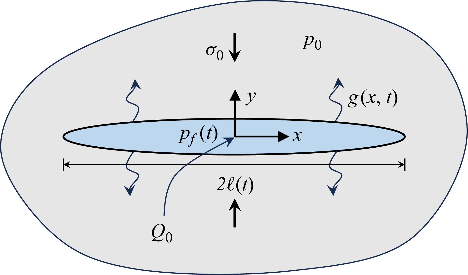


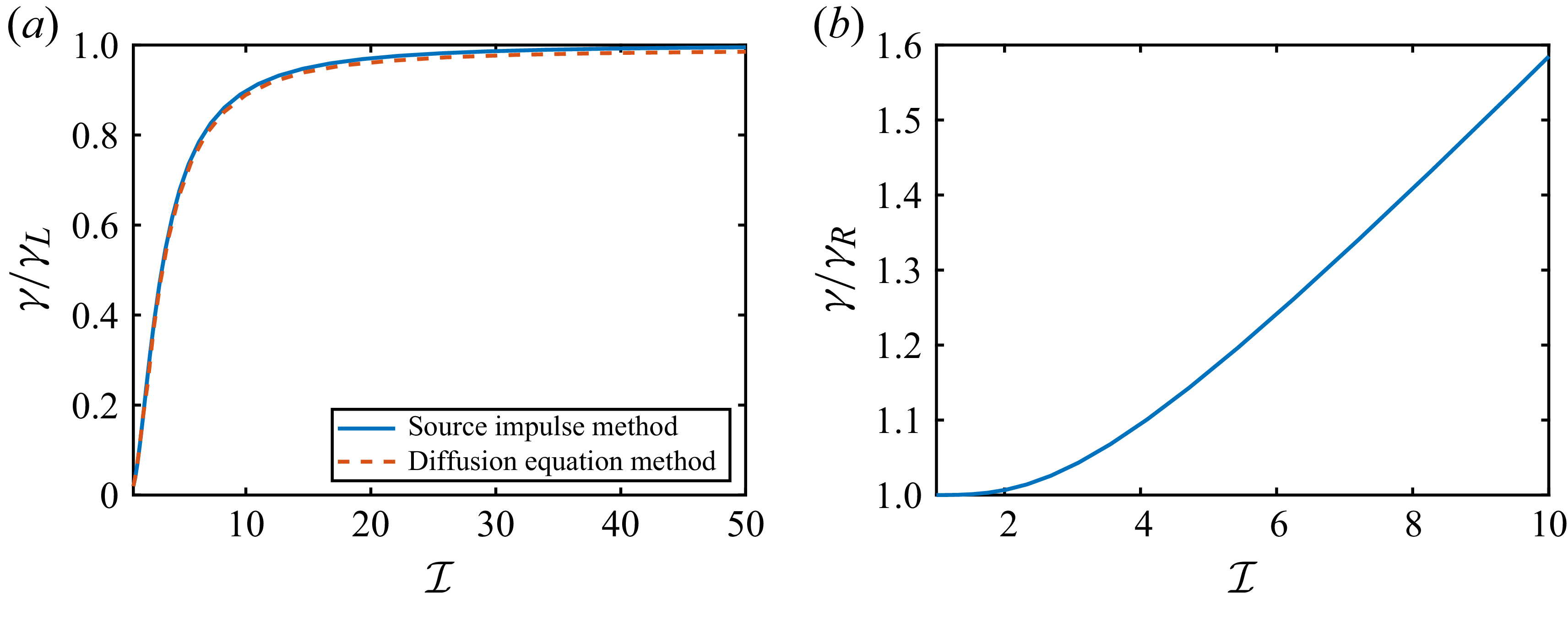


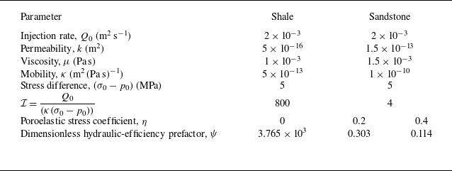
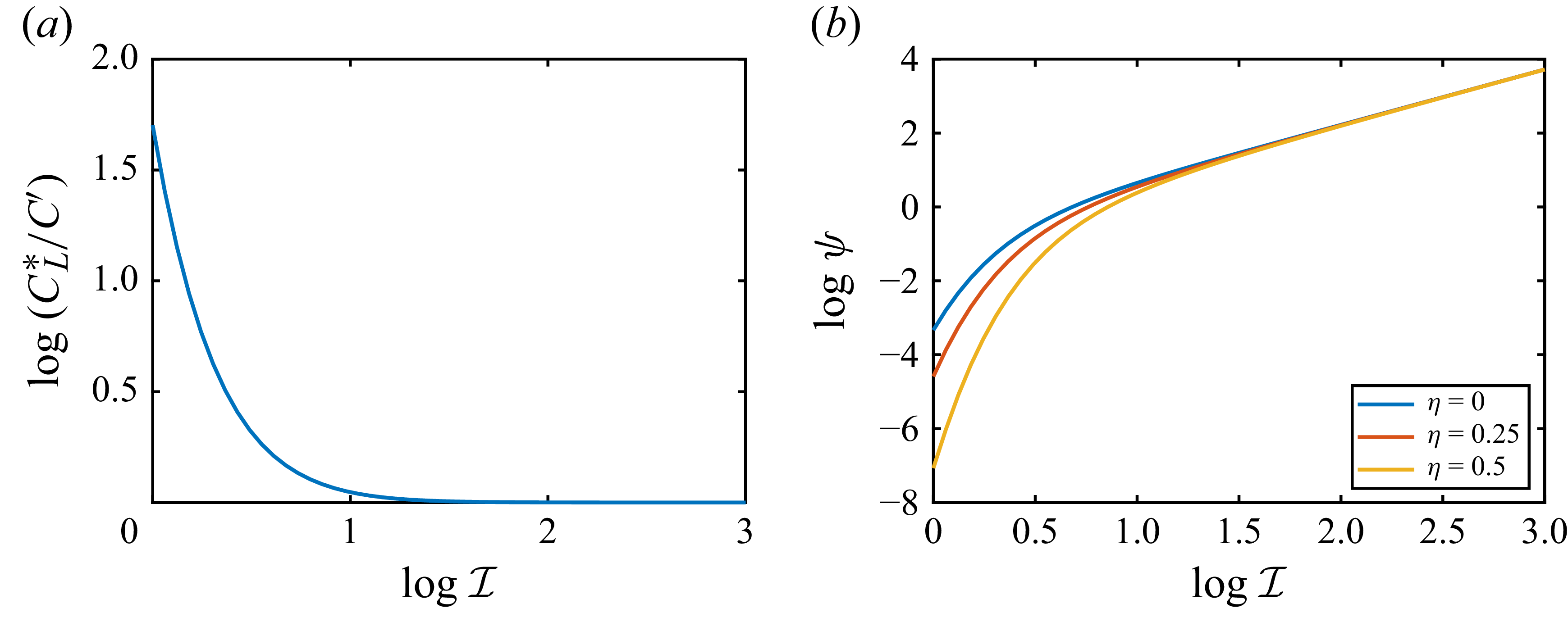


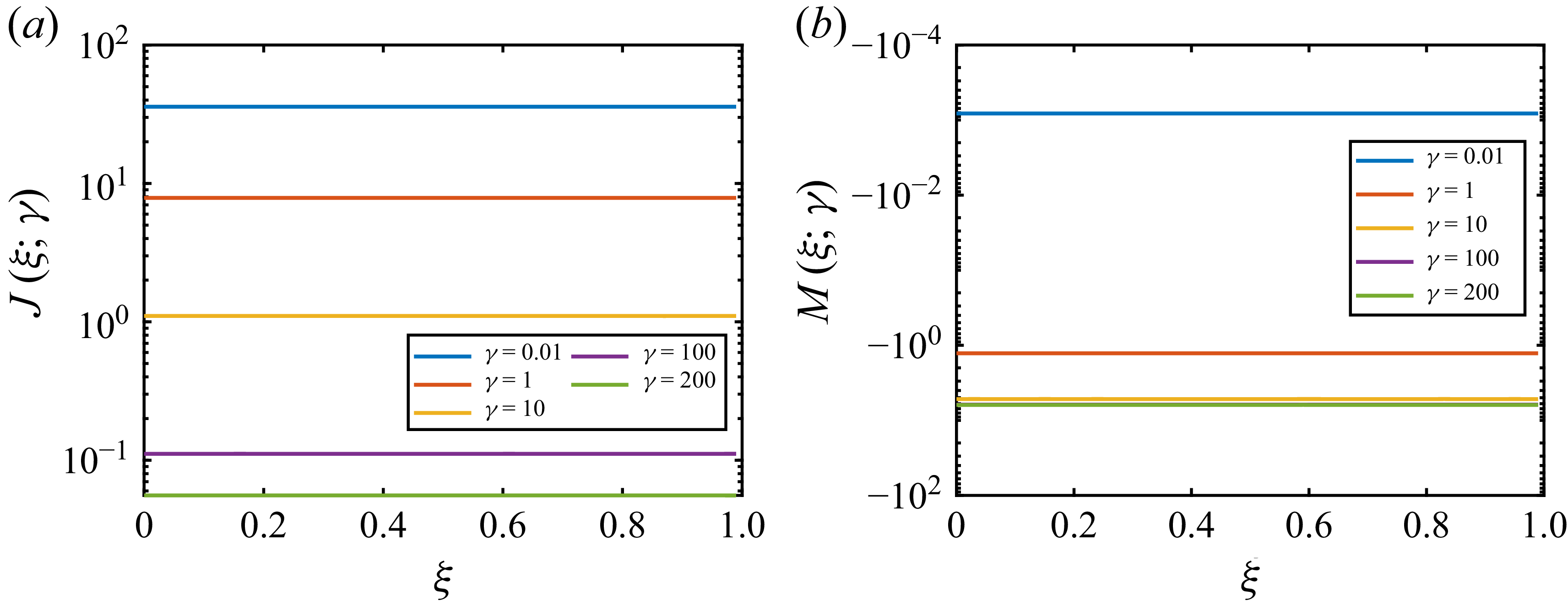


 Open access