


1. Introduction
Everyday experience teaches that radially convergent flows close to a liquid surface produce vigorous transient liquid ejections in the form of a jet perpendicular to the surface, as those seen after bubble bursting (Kientzler et al. Reference Kientzler, Arons, Blanchard and Woodcock1954), droplet impact on a liquid pool (Yarin Reference Yarin2006) or cavity collapse (Ismail et al. Reference Ismail, Gañán-Calvo, Castrejón-Pita, Herrada and Castrejón-Pita2018). The mechanical energy of the flow comes from the free surface energy of the initial cavity. Among these processes, bubble bursting can be considered the parametrically simplest and most ubiquitous one: just two non-dimensional parameters, namely the Ohnesorge ( $Oh$) and Bond (
 $Bo$) numbers, determine the physics and the outcome (
 $Oh$ and
  $Bo$, weighting the viscous and gravity forces with surface tension, respectively). It has received special attention in the scientific literature due to its impact at global planetary scales (bubble bursting at the sea surface, e.g. Kientzler et al. (Reference Kientzler, Arons, Blanchard and Woodcock1954), Blanchard & Woodcock (Reference Blanchard and Woodcock1957), Veron (Reference Veron2015) and Sampath et al. (Reference Sampath, Afshar-Mohajer, Chandrala, Heo, Gilbert, Austin, Koehler and Katz2019); disease and pandemic transmission, e.g. Bourouiba (Reference Bourouiba2021)) and in more ‘indulging’ applications (e.g. Ghabache et al. Reference Ghabache, Liger-Belair, Antkowiak and Séon2016; Séon & Liger-Belair Reference Séon and Liger-Belair2017).
Current works state that the subject is already deeply understood (Berny et al. Reference Berny, Deike, Séon and Popinet2020; Sanjay, Lohse & Jalaal Reference Sanjay, Lohse and Jalaal2021), yet despite optimistic statements, even in the simplest case where the liquid properties are constant and the gas-to-liquid density and viscosity ratios are very small, unsettling but crucial questions remain open. Within an ample range of  $Oh$ and
  $Bo$, bubble bursting exhibits a strong focusing effect due to the nearly cylindrical collapse of a main wave at the bottom of the parent bubble. In these cases, a tiny bubble gets trapped and an extremely thin and rapid spout emerges. That initial spout grows into a much taller, thicker and slower transient jet that may eventually expel droplets. Their eventual size and speed is determined by
  $Oh$ and
  $Bo$. However, for an apparently critical
  $Oh$, (
 $Oh^*$), the initial ballistic spout keeps its large speed and extremely thin radius until it ejects a nearly invisible droplet, such that the spout momentum (proportional to its velocity times its volume) seems to vanish. Strikingly, a nearly symmetric behaviour is observed around that
  $Oh^*$ (Séon & Liger-Belair (Reference Séon and Liger-Belair2017), figure 16). Around that special parametrical region, experiments and numerical simulations exhibit a strong dispersion attributed to local viscous effects and interaction with the gas environment (Brasz et al. Reference Brasz, Bartlett, Walls, Flynn, Yu and Bird2018; Dasouqi, Yeom & Murphy Reference Dasouqi, Yeom and Murphy2021).
In general, the global streamlines of the flow resemble a dipole with its axis perpendicular to the interface (figure 1), which is responsible for the vigorous liquid–air transfer process characteristic of this phenomenon (Lee et al. Reference Lee, Weon, Park, Je, Fezzaa and Lee2011). The energy excess of the convergent flow leads to both a fast transient capillary jet and a vortex ring in opposite directions but equivalent effective momenta by virtue of Newton's third law of motion. Their radically different kinematics, due to a large density disparity across the interface, is not an obstacle to their profound symmetry, as we will show here. We claim that this symmetry and its scalings are the keys to determine the eventual ejected droplet size and speed, and the appearance of singular dynamics. In this regard, some of the above cited authors and many others (e.g. MacIntyre Reference MacIntyre1972; Duchemin et al. Reference Duchemin, Popinet, Josserand and Zaleski2002; Thoroddsen et al. Reference Thoroddsen, Takehara, Nguyen and Etoh2018) have noticed the trapping of tiny bubbles after bursting. In particular, the one trapped at the bottom of the formed cavity is the relic of a singularity produced by the collapse of a pilot capillary wave from the rim formed after the upper film rupture (Duchemin et al. Reference Duchemin, Popinet, Josserand and Zaleski2002; Thoroddsen et al. Reference Thoroddsen, Takehara, Nguyen and Etoh2018). This singularity would explain why the range of  $Oh$ numbers where this occurs exhibits the largest ejection speeds and smaller drops.
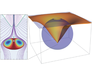
General overview of the flow development around the critical time  $t_0$ of collapse of the main pilot wave at the bottom of the cavity, for
  $Oh = 0.032$,
  $Bo = 0$. The three instants here illustrated are
  $t_0-t=3.54\times 10^{-3}t_c$,
  $t_0-t=8.4\times 10^{-6}t_c$ and
  $t-t_0=4\times 10^{-4}t_c$ (with
  $t_c=(\rho R_o^3/\sigma )^{1/2}$). (a) Global flow streamlines (similar to dipole contours at a liquid–gas surface) showing a particular one (line
  $A$–
$A$– $B$) ending at the point (
 $B$) just above where the collapse eventually occurs. The blue sphere of the three-dimensional rendering is the initial bubble immediately after bursting. (b) Local details of the same instants. The stream function levels shown are closer around the tiny trapped bubble to exhibit the vortex ring. Note that the upper axial point of the ellipsoid defining the vortex ring coincides with the point where the surface collapsed at
  $t=t_0$ and remains at that position: observe the horizontal line connecting the three subpanels of panel (b). The main flow velocities
  $W$ (radial) and
  $V$ (axial, ejection) are indicated. The dashed lines represent the instantaneous stream tube which feeds the collapsing point or the issuing jet. In these simulations using the volume of fluid method (VOF) ( Basilisk, Popinet Reference Popinet2015), the density and viscosity of the liquid is 1000 and 100 times that of the gas, respectively, to reflect similar relations to the air–salt water ones.

In this work, we present: (i) a universal non-trivial scaling of the evolution of the flow kinematic variables (characteristic lengths and velocity); (ii) a prediction of the eventual ejected droplet size and speed, for the complete range of  $Oh$ and
  $Bo$ for which ejection occurs (which generalizes Gañán-Calvo (Reference Gañán-Calvo2017)); and (iii) an explanation why an apparently singular value of
  $Oh^*$ appears. The existing data from prior works (e.g. those collected in Gañán-Calvo (Reference Gañán-Calvo2017); Brasz et al. (Reference Brasz, Bartlett, Walls, Flynn, Yu and Bird2018), Deike et al. (Reference Deike, Ghabache, Liger-Belair, Das, Zaleski, Popinet and Seon2018), Gañán-Calvo (Reference Gañán-Calvo2018) and Berny et al. (Reference Berny, Deike, Séon and Popinet2020)) and novel numerical simulations are compared with our theoretical results. When the droplet size and ejection velocity are properly scaled according to our model, the data show a remarkable collapse around our model except in the vicinity of
  $Oh^*$. A careful inspection reveals that all data from numerical simulations exhibit an enormous degree of dispersion that experimental data do not display. In fact, while numerical series should be independently fitted, the available experimental series appear to obey a single universal fitting to our model. Given that it relies on just two non-dimensional parameters alone,
  $Oh$ and
  $Bo$, this has a twofold consequence: (i) it highlights the critical importance of the artificial initial conditions after film bursting in the numerical simulations among the different authors, which precludes universality; and (ii) it provides a proof that the natural process should be fundamentally universal in terms of
  $Oh$ and
  $Bo$ alone, as expected from the universality of initial film drainage and rupture (Eggers & Fontelos (Reference Eggers and Fontelos2015) and references therein), which supports the universal validity of our model once the three proposed physically relevant fitting parameters are found.
2. Formulation and dynamical scaling analysis
Consider a gas bubble of initial radius  $R_o$ very close or tangent to the free surface of a liquid with density, surface tension and viscosity
  $\rho$,
  $\sigma$ and
  $\mu$, respectively, in static equilibrium under a relatively small action of gravitational acceleration
  $g$ normal to the free surface far from the bubble. The flow properties are considered constant. At a certain instant, the thin film at the point of tangency breaks and the process of bubble bursting starts (figure 1a). The problem is thus determined by the Ohnesorge (
 $Oh = {\mu }/{(\rho \sigma R_o)^{1/2}}$) and Bond (
 $Bo = {\rho g Ro^2}/{\sigma }$) numbers alone (Montanero & Gañán-Calvo Reference Montanero and Gañán-Calvo2020). Alternatively, instead of
  $Oh$, some authors prefer to use the Laplace number (
 $La$), which is simply
  $La = Oh^{-2}$ (e.g. Duchemin et al. Reference Duchemin, Popinet, Josserand and Zaleski2002; Lai, Eggers & Deike Reference Lai, Eggers and Deike2018). Also, the Morton number,
  $Mo = Bo\, Oh^4$, has been used as a relative measure of the gravitational forces (e.g. Berny et al. Reference Berny, Deike, Séon and Popinet2020). The liquid rim that is initially formed pilots two main capillary wavefronts, one that advances along the bubble surface towards its bottom, and the other propagating away from the cavity. In some parametrical regions of the domain (Oh, Bo) of interest, a significant fraction of the energy content in the nonlinear wave spectrum of the initial surface configuration (after the bubble film burst) is in the small-wavelength domain (wavelets). For small
  $Oh$, these wavelets may arrive first to the bottom, but they do not produce any significant effect compared with the collapsing main wave (Gañán-Calvo Reference Gañán-Calvo2018) in the parametrical realm considered here. When the main wavefront approaches the bottom, it becomes steep. If the wavefront leads to a nearly cylindrical collapsing neck in a certain region, a tiny bubble gets trapped below the surface once the ejection process commences. The process of radial collapse and bubble trapping is locally described by the theory of Eggers et al. (Reference Eggers, Fontelos, Leppinen and Snoeijer2007), Fontelos, Snoeijer & Eggers (Reference Fontelos, Snoeijer and Eggers2011) and Eggers & Fontelos (Reference Eggers and Fontelos2015) when a strong asymmetry in the axial direction occurs. However, the asymmetry of bubble trapping here observed leads to an extremely rapid and thin initial ejection in the opposite direction from the trapped bubble.
Figure 1(b) shows three illustrating instants of the flow development around the critical instant  $t_0$ at which the axial speed of the liquid surface on the axis reaches its maximum (immediately after the tiny gas neck collapses). When
  $t< t_0$, the flow is predominantly radial (spherical) with a characteristic speed
  $W$ at the interface. After collapse (
 $t>t_0$), while the main flow keeps running radially with speed
  $W$, the axial asymmetry of the flow and the kinetic energy excess of the liquid is axially diverted in the two opposite directions, with radically different results: (i) towards the open gas volume, producing the liquid spout with speed
  $V$ and characteristic radial length
  $R$; and (ii) towards the liquid bulk, as a backward reaction vortex ring (figure 1b, in colours) with characteristic length
  $L$, around the trapped microbubble. Eventually, the advancing front of the resulting capillary jet expels a droplet or droplet train with characteristic radius
  $R$.
$R$.
Obviously, all scales (W, V, R, L) are time-dependent along their evolution. Some relevant prior works (e.g. Zeff et al. Reference Zeff, Kleber, Fineberg and Lathrop2000; Lai et al. Reference Lai, Eggers and Deike2018) have analysed the time self-similarity of the flow variables. Assuming that those time self-similarities exist, our focus is here to obtain closed relationships among those scales and to predict the size and speed of ejections reflected by the eventual values of  $R$ and
  $V$ at the end of the process. This approach, though, demands the identification of the key symmetries appearing in the problem that may lead to an effective problem closure (Gañán-Calvo, Rebollo-Muñoz & Montanero Reference Gañán-Calvo, Rebollo-Muñoz and Montanero2013). To this end, a set of relations among the radial and axial characteristic lengths and velocities was formulated in Gañán-Calvo (Reference Gañán-Calvo2017, Reference Gañán-Calvo2018) on the basis that inertia, surface tension and viscous forces should be comparable very close to the instant of collapse of the free surface. Under the light of detailed numerical simulations, the previously proposed simplified models are put into perspective after a rigorous derivation of the new model. Following a similar rationale to that in Gañán-Calvo (Reference Gañán-Calvo2017), this derivation is made in two steps: (i) we obtain explicit relationships among the four time-dependent variables along the process, verifying their validity numerically; and (ii) we close the problem identifying the critical key factors on the energy balance of the process. The final model is compared with the ample set of experimental and numerical available data, and its validity is extended to the whole range of
  $Oh$ numbers where ejection takes place.
2.1. Instantaneous scalings of kinematic variables along the process
The general momentum equation of the liquid can be written as
 \begin{equation} \rho \boldsymbol{v}_t+
\boldsymbol{\nabla}(\rho \boldsymbol{v}^2 /2 + p - P_a
+ \rho g z)=\rho \boldsymbol{v}\wedge\boldsymbol{\nabla}\wedge
\boldsymbol{v}+\mu \nabla^2 \boldsymbol{v},
\end{equation}
\begin{equation} \rho \boldsymbol{v}_t+
\boldsymbol{\nabla}(\rho \boldsymbol{v}^2 /2 + p - P_a
+ \rho g z)=\rho \boldsymbol{v}\wedge\boldsymbol{\nabla}\wedge
\boldsymbol{v}+\mu \nabla^2 \boldsymbol{v},
\end{equation}
where  $\boldsymbol {v}$ is the velocity vector, subscript
  $t$ denotes a partial derivative with time,
  $p$ is the liquid pressure,
  $z$ the axial coordinate and
  $P_a$ the static gas pressure. Equation (2.1) can be multiplied by the unit vector
  ${\boldsymbol l}$ tangent to any instantaneous streamline, in particular the streamline flowing through a point
  $A$ where it meets the free surface to a point
  $B$ at the vicinity of the point of collapse (see figure 1a). Integrating with respect to the streamline coordinate
  $s$ from
  $A$ to
  $B$ yields
 \begin{equation} \rho \int_A^B {\boldsymbol l}\boldsymbol{\cdot} \boldsymbol{v}_t \,\text{d}s + \left. \rho \boldsymbol{v}^2 /2\right|_B + \left.\sigma \boldsymbol{\nabla}\boldsymbol{\cdot} \boldsymbol{n}\right|_B +\left. \rho g \Delta z\right|_A^B=\mu \int_A^B {\boldsymbol l}\boldsymbol{\cdot} \nabla^2 \boldsymbol{v}\,\text{d}s, \end{equation}
since the velocity is negligible and pressure is  $P_a$ at the point
  $A$. Here,
  $\boldsymbol{n}$ is the unit normal on the liquid surface, and
  $\Delta z$ is the depth of point
  $B$ respect to
  $A$. As a general consideration, the liquid velocities are very small everywhere compared with those at distances
  $L$ to the collapsing region, which may exhibit a self-similar flow structure (Zeff et al. Reference Zeff, Kleber, Fineberg and Lathrop2000; Duchemin et al. Reference Duchemin, Popinet, Josserand and Zaleski2002; Lai et al. Reference Lai, Eggers and Deike2018). The length scale
  $L$ also characterizes the inverse of the mean local curvature of the liquid surface around the region of collapse, for any given time
  $t$. Thus,
  $L$ obviously changes with time around the instant of collapse. To look for symmetries around
  $t_0$, let us consider two situations, one for
  $t< t_0$ and the other for
  $t>t_0$ such that their characteristic length scales
  $L$ are the same (see figure 1). Then, one may estimate the characteristic values of each term of (2.2) for both
  $t< t_0$ and
  $t>t_0$. In any case, the first two terms of (2.2) are always of the same order for this unsteady problem.
For  $t< t_0$, both the left-hand integral and the kinetic energy term at
  $B$ in (2.2) should scale as
  $\rho W^2$. The surface tension term at
  $B$ should be proportional to
  $\sigma /L$, and the gravity term to
  $\rho g R_o$. Finally, the curvature of streamlines suggests that the viscous stresses should scale as
  $\mu W/L$, which fixes the scale of the right-hand side term of (2.2). This is so because boundary layers cannot be thinner than the scale
  $L$ of the collapsing main wave, as shown by Gañán-Calvo (Reference Gañán-Calvo2018): due to the near-zero tangential viscous stress at the free surface, boundary layers cannot be maintained by other means than the internal inertia. In effect, at the vicinity of the surface, there are no other sources of momentum and no other concentrated sources for viscous diffusion than the internal flow, whose fate is dictated by the free surface geometry and, consequently, its energy content. Since that characteristic length
  $L$ is fixed by the collapsing main wave, this should be the minimum (if any) characteristic length of viscous diffusion as well. Thus, the overall scaling balance of (2.2) can be expressed as
 \begin{equation} \rho(W^2+\beta_1 g\,R_o)\sim \sigma\, L^{{-}1}+\alpha_1 \mu\, W\, L^{{-}1}, \end{equation}
where prefactors  $\alpha _1$ and
  $\beta _1$ should be universal constants reflecting the dominance or subdominance of the corresponding terms. Using the natural length and velocity,
  $\ell _\mu =\mu ^2/(\rho \sigma )$ and
  $v_\mu =\sigma /\mu$, respectively, and defining
  $\zeta =L/\ell _\mu$,
  $\omega =W/v_\mu =$ and
  $\epsilon _1=\beta _1 Oh^2{Bo}$, this equation can be written as
 \begin{equation} \omega^2+\epsilon_1 \sim \left(1+\alpha_1 \omega \right)\zeta^{{-}1}. \end{equation}
When  $t>t_0$, the vigorous ejection in the axial direction generates the new characteristic velocity
  $V$ and radial size
  $R$ scales of the liquid jet. The physical symmetry around
  $t_o$ should keep the scale of the radial velocity
  $W$ in the bulk and the spatial scale
  $L$ (including the axial scale of the jet) the same: see the central subpanel in figure 1(b) for
  $Oh = 0.032$,
  $Bo = 0$. Even before collapse, the flow develops a stagnant region in the liquid just below the collapsing point. From this point, a vortex ring of characteristic (growing) size
  $L$ and speed
  $W$ like those beautifully described by Maxworthy (Reference Maxworthy1972) develops; see figure 4 of his work (dissecting absolute and relative speeds is not trivial in these flows, as Maxworthy showed). By virtue of total energy preservation and assuming that the trapped microbubble is much smaller than the vortex, the mechanical energy of the vortex,
  $\rho W^2L^3$, should mirror that of the vigorous microjet,
  $\rho V^2 R^2 L$. Furthermore, the streamlines below the jet form a feeding stream tube coming from deep in the liquid domain (surrounding the vortex ring, see figure 1b, right-hand subpanel), which should ultimately originate far away from the bubble at the free surface. In contrast, Gordillo & Rodriguez-Rodriguez (Reference Gordillo and Rodriguez-Rodriguez2019) ignores such a vortex and proposes a simplified radial (cylindrical) flow model, which hampers the correct identification of the local flow scales.
In summary, one can write
 \begin{equation} \rho V^2 R^2 L \sim \rho W^2 L^3\Longrightarrow V\,R\sim W\,L\Longrightarrow \upsilon\, \chi\sim \omega\, \zeta, \end{equation}
where  $\chi =R/\ell _\mu$ and
  $\upsilon =V/v_\mu$. As a secondary consequence, the incoming conical flow raises the conical surface at characteristic speed
  $W$.
$W$.
One can now estimate the scaling of the different terms of (2.2) for a streamline ending at a point  $B$ at the surface of the jet (see figure 1a), and write the following balance:
 \begin{equation} \rho(V^2+\beta_2 g\,R_o)\sim \sigma\, R^{{-}1} + \alpha_2 \mu W\, L^{{-}1}, \end{equation}
where, again, prefactors  $\alpha _2$ and
  $\beta _2$ should be universal constants at the end of the process. Using natural scales and defining
  $\epsilon _2=\beta _2 {Oh}^2{Bo}$, (2.6) reads
 \begin{equation} \upsilon^2+\epsilon_2 \sim \chi^{{-}1}+ \alpha_2 \omega \zeta^{{-}1}. \end{equation}
 As in Gañán-Calvo (Reference Gañán-Calvo2017), (2.4), (2.5) and (2.7) define three relationships between the time dependent scales  $(\chi, \upsilon, \zeta, \omega )$. In effect, an explicit relationship between
  $\omega$ and
  $\zeta$ is easily derived after rewriting (2.4):
 \begin{align} (\omega \zeta)^2 - \alpha_1 (\omega \zeta) +\zeta (\epsilon_1 \zeta -1) \sim 0 \quad \Rightarrow \quad \omega \zeta \sim \varphi \equiv \frac{\alpha_1}{2} + \left[\left(\frac{\alpha_1}{2} \right)^2+\zeta(1-\epsilon_1 \zeta)\right]^{1/2}. \end{align}
Also, introducing (2.5) and (2.8) in (2.7), the following relationship between  $\upsilon$ and
  $\zeta$ results:
 \begin{align} (\varphi \upsilon)^2 \,{-}\, (\varphi \upsilon) +\varphi^2 (\epsilon_2 \,{-}\, \alpha_2 \varphi \zeta^{{-}2}) \,{\sim}\, 0 \quad \!\Rightarrow\! \quad \varphi \upsilon \,{\sim}\, \phi \equiv \frac{1}{2} \,{+}\, \left[\frac{1}{4} + \varphi^2 \left( \frac{\alpha_2 \varphi}{\zeta^{2}}\,{-}\,\epsilon_2 \right) \right]^{1/2}. \end{align}
In summary, the following explicit relationships hold:
 \begin{equation} \chi \sim \varphi^2 \phi^{{-}1},\quad \upsilon \sim \varphi^{{-}1}\phi,\quad \omega \sim \varphi/\zeta, \end{equation}
which can be tested against numerical simulations. For  $\alpha _1\rightarrow 0$,
  $\alpha _2\gg 1$ and
  $\epsilon _{1,2}=0$, (2.10a–c) yields
  $\chi \sim \upsilon ^{-5/3}$,
  $\zeta \sim \upsilon ^{-4/3}$ and
  $\omega \sim \upsilon ^{2/3}$, as predicted by Gañán-Calvo (Reference Gañán-Calvo2017). However, given that the ejection is fundamentally a ballistic (inertial) process, one may expect two possible regimes in the evolution of the ejection.
(i) When
 $|t-t_0|< t_\mu =\mu ^3/(\rho \sigma ^2)$, the inertia and viscous forces should be dominant ($\alpha _{1,2}\gg 1$). In this case, for $Bo = 0$, $\chi \sim \zeta \sim \upsilon ^{-1}\sim \omega ^{-1}$.
(ii) For
$|t-t_o|>t_\mu$, inertia and surface tension forces should prevail ($\alpha _{1,2}\ll 1$). Here, if $Bo = 0$, one obtains $\chi \sim \zeta \sim \upsilon ^{-2} \sim \omega ^{-2}$, consistently with Zeff et al. (Reference Zeff, Kleber, Fineberg and Lathrop2000).


Observe that  $\chi \sim \zeta$ and
  $\upsilon \sim \omega$ always hold.
Testing the validity of (2.10a–c) involves showing that the two limits (i) and (ii) and their corresponding scaling relationships are indeed reached as the time-dependent characteristic scales  $(\chi, \zeta, \upsilon, \omega )$ evolve along the process. To do so, we analyse their evolution from numerical simulation (momentum-conserving VOF, Basilisk code). We have recorded the time-dependent values of the maximum radius of curvature in the meridional plane at the point of maximum radial velocity of the interface, and the radius of curvature and velocity of the jet front on the jet axis to represent the time-dependent characteristic values of
  $L$,
$L$,  $R$ and
  $V$, respectively, for
  $t>t_0$ (no scales of
  $R$ and
  $V$ appear before ejection, i.e. for
  $t< t_0$). Since (2.10a–c) does not provide the time dependencies of the variables, in figure 2(a–c) we plot the non-dimensional evolving values of
  $\chi$ versus
  $\zeta$,
  $\omega$ versus
  $\upsilon$ and
  $\chi$ versus
  $\upsilon$, respectively, for a detailed range of
  $Oh$ numbers.
Numerical data (momentum-conserving VOF, Basilisk, minimum cell size  $3\times 10^{-4}R_o$ for this figure) compared with prediction (2.10a–c). The
  $Oh$ numbers of the different series are given at the right-hand side of the figure. (a) Plot of
  $\chi$ versus
  $\zeta$. Black dashed line (
 $\chi \sim \zeta$) shows the essential proportionality between both spatial variables along the whole process as predicted, consistently with prior analyses (Zeff et al. Reference Zeff, Kleber, Fineberg and Lathrop2000). (b) Plot of
  $\upsilon$ versus
  $\omega$. Black dashed line (
 $\upsilon \sim \omega$) also shows the proportionality between both variables for
  $\upsilon$ below 20; the deviation above that value reflects the very high initial velocity acquired by the spout front at its inception for
  $Oh$ around
  $Oh^*$ (focusing effect). (c) Plot of
  $\chi$ versus
  $\upsilon$. The black dashed line is the theoretical prediction for
  $t-t_o >t_\mu$ (
 $\alpha _{1,2}\rightarrow 0$), which yields
  $\chi \sim \upsilon ^{-2}$. The blue dashed line would correspond to
 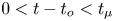 $0< t-t_o < t_\mu$, with
  $\alpha _{1,2}\gg 1$, yielding
  $\chi \sim \upsilon ^{-1}$. Observe the visible change of regime in the case
  $Oh = 0.038$ around
  $\chi \simeq 0.65$, i.e. around
  $R \simeq 0.65 \ell _\mu$. The scaling law proposed by Gañán-Calvo (Reference Gañán-Calvo2017),
  $\chi \sim \upsilon ^{-5/3}$, is also plotted as a red dashed line.

Firstly, figure 2(a) demonstrates the fundamental proportionality between  $\zeta$ and
  $\chi$ along the whole process, as anticipated. In this regard, the small constant of proportionality between both scales,
  $\chi \simeq 0.03 \zeta$, should be noticed. The importance of this observation will be apparent after the global assessment of the energy balance of the process in § 2.2.
Secondly, the remarkable collapse of the curves of  $\chi$ versus
  $\upsilon$ in figure 2(c) reveals the two clear regimes as anticipated: viscosity-dominated (
 $\alpha _{1,2}\gg 1$) when
  $\chi \lesssim 1$ (
 $R \lesssim \ell _\mu$) and surface tension-dominated (
 $\alpha _{1,2}\rightarrow 0$) when
  $\chi \gtrsim 1$ (
 $R \gtrsim \ell _\mu$), corresponding to
  $\chi \sim \upsilon ^{-1}$ and
  $\chi \sim \upsilon ^{-2}$, respectively. The robustness of the results is thus confirmed: the formation and pinch-off of a droplet is expected to take place once surface tension becomes important, resulting in a dependency as observed. The relatively small deviations from the theoretical prediction (2.10a–c) for the smallest and largest values of
  $\upsilon$ in figure 2(c) reflect the vibrations of the droplet about pinch-off and ejection (not considered here) and the very initial evolution just after
  $t=t_0$, respectively.
2.2. Energy balance
For a given  $Bo$ that fixes the initial static geometry of the bubble, droplet ejection is prevented by the loss of mechanical energy above a certain
  $Oh$ threshold value. In the absence of gravitational forces (
 $Bo \simeq 0$), a reported value of that threshold is
  $Oh_{th}$ = 0.052 (Lee et al. Reference Lee, Weon, Park, Je, Fezzaa and Lee2011). Below that threshold, the finest and fastest jets and droplets are observed for a certain value
  $Oh^* < Oh_{th}$. Therefore, to close the problem, a key question which is not resolved by (2.10a–c) is the mechanical energy available to perform the ballistic ejection close to
  $t_o$. One can express the mechanical energy equation in a sufficiently ample fluid volume
  $\varOmega (t)$ around the initial bubble from the instant of bubble bursting (
 $t=0$) up to the point of collapse
  $t_o$. The fluid volume
  $\varOmega (t)$ can be formed by the free surface and a hemisphere around the cavity with a radius approximately twice or three times larger than
  $R_o$ (see figure 3):
 \begin{equation} \left. \int_{\varOmega(t')}\rho\left(\boldsymbol{v}^2/2+gz\right)\,\text{d} \varOmega \right|_{t=0}^{t_0}=\int_{t=0}^{t_0} \int_{S(t')} \boldsymbol{v}\boldsymbol{\cdot} \left( {\boldsymbol\tau'} -p\boldsymbol{I} \right) \boldsymbol{\cdot} \boldsymbol{n}\, \text{d} A\, \text{d} t' ,\end{equation}
where  ${\boldsymbol \tau '}$ is the viscous stress and
  $\boldsymbol {I}$ the identity matrix. The surface of the integral domain is
  $S(t)={\mathcal {D}}_1(t) + {\mathcal {D}}_2$, where
  ${\mathcal {D}}_2$ is a hemisphere with a fixed radius. We define the capillary velocity as
 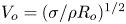 $V_o = ({\sigma }/{\rho R_o})^{1/2}$, which is the global expected value of the average velocities along the process.
The control volume  $\varOmega (t)$ bounded by the free surface
  ${\mathcal {D}}_1$ and the fixed hemispherical surface
  ${\mathcal {D}}_2$, considered for the integral representation of the mechanical energy balance, close to
  $t_0$.

Observing the geometric configuration of streamlines in figure 1, the most relevant feature is a stream tube which ends up at the collapse point, coming from below (figure 1b – subsequently also shown in figure 6). This stream tube, with velocity  $W$ and cross-sectional area proportional to
  $L^2$, would ultimately feed the ejection. The global view of the streamlines’ configuration in figure 1(a) reveals that the characteristic length of that stream tube is indeed
  $R_o$, since its configuration remains practically unaltered along the process sufficiently far from the collapse region. Thus, the kinetic energy term should be proportional to
 \begin{equation} \left. \int_{\varOmega(t')} (\rho\boldsymbol{v}^2/2) \, \text{d} \varOmega \right|_{t=0}^{t} \sim \rho W^2 \times L^2 \, R_o. \end{equation}
Note that the initial kinetic energy is zero. If one neglects viscous and gravity works, expression (2.11) suggests the scaling
 \begin{equation} \rho W^2 L^2 R_o \sim \sigma R_o^2 \sim \rho V_o^2 R_o^3 = \text{const.} \Rightarrow W L \sim V_o R_o, \end{equation}
which together with the scaling previously obtained as  $W L \sim V R$ after collapse, it would suggest
  $V R \sim V_o R_o$. This relationship was already observed by Duchemin et al. (Reference Duchemin, Popinet, Josserand and Zaleski2002) and Ghabache et al. (Reference Ghabache, Antkowiak, Josserand and Séon2014), among others, for negligible viscosity and gravity. However, it does not faithfully describe the nonlinear behaviour observed for
  $Oh$ around
  $Oh^*$: note that in the vicinity of
  $Oh^*$ the product
  $V R$ becomes much smaller than
  $V_o R_o$ (Duchemin et al. Reference Duchemin, Popinet, Josserand and Zaleski2002; Walls, Henaux & Bird Reference Walls, Henaux and Bird2015; Ghabache & Séon Reference Ghabache and Séon2016; Gañán-Calvo Reference Gañán-Calvo2017; Séon & Liger-Belair Reference Séon and Liger-Belair2017; Deike et al. Reference Deike, Ghabache, Liger-Belair, Das, Zaleski, Popinet and Seon2018). There is not a general consensus around the value of
  $Oh^*$ and the origin of this behaviour. Naturally,
  $Oh^*$ depends on the Bond number through the initial shape of the bubble before bursting, since that shape determines the detailed dynamic path of the process. Reducing that geometry to a sphere, i.e.
  $Bo \simeq 0$, the simulations presented here and those of Berny et al. (Reference Berny, Deike, Séon and Popinet2020) and Deike et al. (Reference Deike, Ghabache, Liger-Belair, Das, Zaleski, Popinet and Seon2018) agree on
  $Oh^* \simeq 0.03$; in contrast, Gañán-Calvo (Reference Gañán-Calvo2017) suggests
  $Oh^* \simeq 0.043$, in the range that would roughly point to Duchemin's data. Therefore, a detailed analysis of the process of collapse is needed, in particular the effects of microbubble trapping and the onset of ejection at the time singularity represented by
  $t_0$ (if such a singularity occurs).
2.2.1. The nonlinear behaviour around $Oh^*$: focusing, bubble trapping and the start of ejection

Previous works (Duchemin et al. (Reference Duchemin, Popinet, Josserand and Zaleski2002), Ghabache et al. (Reference Ghabache, Antkowiak, Josserand and Séon2014) and Deike et al. (Reference Deike, Ghabache, Liger-Belair, Das, Zaleski, Popinet and Seon2018), among others) have postulated that the origin of these ballistic ultrafast jets is a finite-time singularity event at  $Oh^*$. In reality, a true singularity followed by an instantaneous ultrafast jet occurs in all instances where a capillary wave collapses nearly cylindrically at the bottom of the cavity, locally resembling the bubble collapse phenomenon described by Eggers & Fontelos (Reference Eggers and Fontelos2015). However, given the geometrical asymmetry of that collapse in the axial direction (see figure 4a), its consequences are twofold.
(a) Bubble trapping about collapse for an ample range of  $Oh$ numbers. The origin of the axial scale has been arbitrarily located 0.001 times
  $R_o$ above the point where collapse occurs in all cases. (b) Length
  $L_b$ of the trapped bubble at collapse, as a function of
  $Oh$. Numerical results performed with a spatial precision below
  $0.02\ell _\mu$. Interestingly, the reported
  $Oh^*$ values correspond to the range where the growth in size of the trapped bubble as a function of
  $Oh$ becomes maximum (i.e.
  $Oh$ around 0.033).

(i) A microbubble gets trapped. The dependence of its size on
$Oh$ is summarized in figure 4 for an ample range of $Oh$ numbers.(ii) More importantly, an extremely thin ligament of vanishing radial size and very large speed is ballistically emitted in the opposite axial direction from the tiny trapped bubble, as illustrated in figure 5. As discussed in § 2, a vortex ring (usually much larger than the tiny trapped bubble) with a global mechanical energy equivalent to that of the ejected liquid spout is emitted towards the liquid bulk (see figure 1) to keep the overall neutrality of the initial axial momentum (which can be termed a bazooka effect).


Initial instants after collapse and the start of ejection for  $Oh = 0.03$, in steps
  $\Delta t=0.74 \, t_\mu$. The axes length scale is
  $R_o$ to show the smallness of the region analysed. The left-hand inset shows the spout geometry (front radius of curvature approximately 0.15
 $\ell _\mu$) at
  $t-t_0=0.2 t_\mu$, showing the recoiling trapped microbubble. The right-hand inset illustrates the competing effects of ballistic ejection and recoil. Numerical results performed with a spatial precision below 0.02
 $\ell _\mu$.

The described phenomenon of microbubble entrapment and initial ejection can even occur with smaller collapsing waves before the main wave generates the more energetic dominant ejection that eventually overwhelms the former ones (Duchemin et al. Reference Duchemin, Popinet, Josserand and Zaleski2002; Deike et al. Reference Deike, Ghabache, Liger-Belair, Das, Zaleski, Popinet and Seon2018; Gañán-Calvo Reference Gañán-Calvo2018). However, the total mechanical energy of that initial singular spout is quite small, and surface tension together with axial dissipation immediately blunts it (figure 5) in a self-similar fashion described by Eggers's theory (Eggers Reference Eggers1993). This blunting is equivalent to the ultrafast recoil of a liquid ligament after pinch-off, as observed from a framework moving axially with a large ballistic convective velocity from the pinching point (see figure 5 for  $Oh = 0.03$). As far as sufficient mechanical energy is left after collapse, the spout will grow in size (scaling as
  $\chi$) and decrease in speed (scaling as
  $\upsilon$), while keeping the scaling relationships (2.10a–c) previously analysed. This growth continues until a droplet is formed by surface tension at the front of the spout.
What happens at  $Oh^*$ has been termed a focusing effect (Deike et al. Reference Deike, Ghabache, Liger-Belair, Das, Zaleski, Popinet and Seon2018) of the global evolution around collapse. However, its physical understanding requires further consideration. Figure 6 shows the cases
  $Oh = 0.026$, 0.033 and 0.047 just at the onset of ejection (figure 6a–c) and when the length of the liquid ligament is a fixed fraction of
  $R_o$ (approximately
  $0.27R_o$, figure 6d–f). The stream tube that meets the free surface with zero radial velocity is highlighted as a red thick line. This figure shows that the size of the vortex ring just after collapse is much larger when
  $Oh$ is around
  $Oh^*$. A detailed observation of the streamlines reveals that the presence of the trapped cavity is associated with the formation of the vortex ring even before collapse when
  $Oh$ is around
  $Oh^*$: note that the vortex streamlines originate at the front of the advancing trapped cavity and flow backward, terminating at the rear of the cavity (see figure 6b). As a consequence of the early formation of that backward vortex ring of maximum size, the energy left for ejection immediately after collapse when
  $Oh = Oh^*$ is the minimum on the whole
  $Oh$ range.
Focusing effect: configuration of streamlines just after collapse (a–c) and when the jet is around 0.27 $R_o$ in length, for the three illustrative
  $Oh$ numbers indicated. The stream tube that meets vertically (zero radial velocity) the free surface is highlighted as a red thick line.

The detailed phenomenon just described does not hamper the overall maintenance of the axial momentum balance. In fact, a vortex ring is always formed (see figure 6d–f). However, as explained, the total mechanical energy left for raising the ejected liquid column becomes minimized for  $Oh$ around
  $Oh^{\ast}$. This is consistent with the fact that the cross-section of the stream tube which feeds the liquid column keeps smaller along the process when
  $Oh$ is around
  $Oh^*$ (see figure 6e). However, the fact that the total remaining mechanical energy is minimal does not imply that the local mechanical energy per unit volume in the ejected ligament must also be minimal. Quite on the contrary, that energy per unit volume is maximized, since the cross-sectional size and thus the total volume of liquid to be pushed is markedly minimized. Consequently, the initial pilot spout can remain ballistic for a longer time just after collapse. The radial scale of that pilot spout, comparable to that of the front of the stream tube responsible for the ejection feed, should be
  $\ell _\mu$, which is the natural spatial scale selected when inertial, viscous and surface tension forces dominate locally (Eggers Reference Eggers1993). All this is confirmed by our numerical simulations, where we use a spatial precision an order of magnitude smaller than
  $\ell _\mu$ to adequately resolve the finest details of the ejection.
When  $Oh > Oh^*$, though, viscous dissipation takes over, which causes the widening of the emitted spout. Besides, for very small
  $Oh$ numbers when no bubble trapping occurs, the sheer curvature reversal of the bubble bottom and the appearance of a stagnation point below the surface guarantee the ejection. This occurs even in the absence of bubble trapping and the initial vigorous pilot emission just described, due to the large overall excess energy remaining in the absence of any significant viscous dissipation.
2.2.2. Final energy balance including viscous dissipation
The observed deviation of  $V R$ from its expected (inviscid) value
  $V_o R_o$ can be quantified expressing the counterpart of (2.11) after collapse as
 \begin{equation} \left. \int_{\varOmega(t')}\rho\left(\boldsymbol{v}^2/2+gz\right)\,\text{d} \varOmega \right|_{t_0}^{t}=\int_{t_0}^{t} \int_{S(t')} \boldsymbol{v}\boldsymbol{\cdot} \left( {\boldsymbol\tau'} -p\boldsymbol{I} \right) \boldsymbol{\cdot} \boldsymbol{n}\, \text{d} A\, \text{d} t'. \end{equation}
The control volume remains the same as that used for (2.11), considering now the highly deformed free surface due to the ejection and possible bubble trapping. While gravity is simply volumetric, proportional to  $(\rho g R_o)R_o^3$ and reflecting the effect of gravity on the initial bubble shape, i.e.
 \begin{equation} \left. \int_{\varOmega(t')} (\rho gz) \, \text{d} \varOmega \right|_{t=0}^{t}\simeq{-}\beta_3 (\rho g R_o) \times R_o^3, \end{equation}
the viscous terms should be proportional to the dominant one, as
 \begin{equation} \int _{t=0}^t \int_{S(t')} \boldsymbol{v} \boldsymbol{\cdot} \tau' \boldsymbol{\cdot} \boldsymbol{n} \, \text{d}A \, \text{d}t' \simeq{-} \alpha_3' (\mu V_o/R_o) \times R_o^2 \times R_o, \end{equation}
where constant  $\alpha _3'$ should be a universal constant at the end of the process, like
  $\alpha _{1,2}$. Note that the average total displacement of fluid particles that this term retains should be proportional to
  $\boldsymbol {v} t_c \simeq R_o$, being
  $\boldsymbol {v} \sim V_o$ and
  $t_c=(\rho R_o^3/\sigma )^{1/2}$. This is so because the main contribution to the integral comes from the larger side
  ${\mathcal {D}}_2$ of the control volume (see figure 3) since the normal viscous stresses on the free surface are at most comparable to the surface tension, which is maximum at the front of the growing spout. Moreover, viscosity is, on the one hand, an energy sink that lowers the energy available for ejection, and on the other, it modifies the interface shape at the instant of collapse, favouring or preventing bubble trapping and overall focusing of the flow as described previously in § 2.2.1.
Finally, the surface tension term can be estimated as
 \begin{equation} -\int_{t=0}^{t} \int_{S(t')} \boldsymbol{v}\boldsymbol{\cdot} p\boldsymbol{I}\boldsymbol{\cdot} \boldsymbol{n}\, \text{d} A\, \text{d} t'\sim k \sigma R_o^2 \times V_o t_c = k \sigma R_o^3. \end{equation}
Given that the integral in (2.17) is in reality the difference between the available surface energy between the instant of collapse and any time after that (in particular, at the end of ejection), one should expect the constant  $k$ to be quite small, since the main energy conversion from the initially available surface energy to kinetic energy has already been performed from
  $t=0$ to
  $t_0$, implying
  $\rho W^2 L^2 R_o^3 \sim \sigma R_o^2$. To this end, one should bear two important considerations in mind: (i) figure 2(b) shows that
  $\upsilon /\omega \simeq O(1)$ at the points where these variables have been evaluated, suggesting
  $\upsilon$ to be comparable in size to
  $\omega$ as expected from basic conservation of momentum at the collapse; and (ii)
  $\chi /\zeta \simeq 0.03$. Interestingly, this number is rather comparable to the experimentally observed
  $Oh^*$ values. Therefore, from (2.12) and (2.17) one may expect
 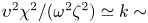 $\upsilon ^2\chi ^2/(\omega ^2\zeta ^2)\simeq k \sim$
  $Oh^{*2}$, which is justified by the relative size between the initial bubble and the ejected droplet.
2.3. Problem closure
While  $\mu V/R$ stays comparable to
  $\rho V^2$ at the start of ejection, viscous forces decelerate the spout until
  $\sigma /R$ becomes strong enough to form a droplet at its tip. Hence, the size of that minimum drop should reflect the ultimate balance between inertia, viscosity and surface tension forces:
 \begin{equation} \rho V^2 \sim \mu V/R \sim \sigma R \quad \Rightarrow \quad R \sim \ell_\mu. \end{equation}
Thus, a minimum surface tension energy proportional to  $(\sigma /\ell _\mu ) \ell _\mu ^2\times R_o$ should necessarily remain available along the process for the emission and formation of that droplet, consistent with experimental observations. In conclusion, keeping that in mind together with (2.17), one can formulate the following scaling of (2.11) at the end of the ejection, when the droplet of radius
  $R$ forms:
 \begin{equation} \rho \left(V^2 R^2 + \beta_3 g R_o^3\right) R_o \sim \sigma R_o^2({{Oh}^*}^2 + \ell_\mu/R_o) - \alpha'_3 \mu V_o R_o^2, \end{equation}
where prefactors  $Oh^*$,
  $\alpha '_3$ and
  $\beta _3$ should be universal positive constants for very small gas-to-liquid density and viscosity ratios. Equation (2.19) is equivalent to the energy equation in Gañán-Calvo (Reference Gañán-Calvo2017), with the exception of the minimum contribution of the surface tension at the natural limit scale
  $\ell _\mu$. Dividing (2.19) by
  $\rho R_o \ell _\mu v_\mu = \mu ^2R_o/\rho$ one gets
 \begin{equation} \upsilon^2 \chi^2 + \beta_3 \frac{{Bo}}{ {Oh}^2} \sim \left[ \left(\frac{{Oh}^*}{{Oh}} \right) ^2 + 1 \right]- \frac{\alpha'_3}{{Oh}}. \end{equation}
2.3.1. Scalings of the ejected droplet size and speed
The right-hand side of (2.20) is a quadratic expression for  $Oh$ with a minimum at
  $Oh = 2{Oh}^{*2}/\alpha '_3$. Observe that this minimum is located exactly at
  $Oh = Oh^*$ if
  $\alpha _3' = 2 {Oh}^*$. Thus, if one defines
 \begin{equation} \alpha_3 = 2 {Oh}^* - \alpha_3', \end{equation}
this parameter would measure both the deviation of the location of the minimum from  $Oh = Oh^*$ and the value of the energy left for ejection. In effect, using definition (2.21), (2.20) reads
 \begin{equation} \upsilon^2 \chi^2 \sim \left( \frac{{Oh}^*}{{Oh}} - 1 \right)^2 + \frac{\alpha_3}{{Oh}} -\beta_3 \frac{{Bo}}{ {Oh}^2}=\varphi^2. \end{equation}
From (2.22) the value of  $Oh$ where
  $R$ is minimum and
  $V$ maximum is given by
 \begin{equation} {Oh}_c=\frac{{{Oh}^*}^2-\beta_3{Bo}}{{Oh}^*-\alpha_3/2}, \end{equation}
around which the dependence is nearly symmetric. When  $Bo = 0$, if
  $\alpha _3$ is sufficiently small,
  $Oh_c\simeq Oh^*$. Therefore,
  $\alpha _3$ constitutes not only a fitting parameter but also a key indicator of the degree of focusing that a certain set of experiments (either physical or numerical) achieve around
  $Oh^*$, as shown in the next section. As we will see next, experiments reveal that
  $\alpha _3\ll Oh^*$, confirming our hypothesis. This fundamental finding explains and justifies the experimental observations by many authors (Duchemin et al. (Reference Duchemin, Popinet, Josserand and Zaleski2002), Walls et al. (Reference Walls, Henaux and Bird2015), Ghabache & Séon (Reference Ghabache and Séon2016), Séon & Liger-Belair (Reference Séon and Liger-Belair2017), Brasz et al. (Reference Brasz, Bartlett, Walls, Flynn, Yu and Bird2018), Deike et al. (Reference Deike, Ghabache, Liger-Belair, Das, Zaleski, Popinet and Seon2018) and Berny et al. (Reference Berny, Deike, Séon and Popinet2020), among others), but not only this: experiments confirm the continuous validity of (2.22) for the whole
  $Oh$ range where droplet ejection occurs.
In addition, one can assume  $\alpha _{1,2}=\beta _{1,2}=0$ for simplicity since (i)
  $\alpha _{1,2}\rightarrow 0$ is a very good approximation, consistent with the fact that surface tension should become dominant when droplet formation and ejection occurs, as previously demonstrated, and (ii) the role of gravity in the expressions (2.4) and (2.7) is expected to be very small compared with inertia and surface tension forces. This is subsequently confirmed by experiments. With these justified simplifications, (2.9) simply reduces to
  $\phi =1$. This finally reduces the scalings (2.8)–(2.10a–c) together with (2.22) to explicit expressions in terms of
  $Oh$ and
  $Bo$ as follows:
 \begin{equation} \left. \begin{gathered}
\chi \sim \left( \frac{{Oh}^*}{{Oh}} - 1 \right)^2 +
\frac{\alpha_3}{{Oh}} -\beta_3 \frac{{Bo}}{ {Oh}^2},\\
\upsilon \sim \left(\left( \frac{{Oh}^*}{{Oh}} - 1
\right)^2 + \frac{\alpha_3}{{Oh}} -\beta_3 \frac{{Bo}}{
{Oh}^2}\right)^{{-}1/2} \end{gathered} \right\} . \end{equation}
\begin{equation} \left. \begin{gathered}
\chi \sim \left( \frac{{Oh}^*}{{Oh}} - 1 \right)^2 +
\frac{\alpha_3}{{Oh}} -\beta_3 \frac{{Bo}}{ {Oh}^2},\\
\upsilon \sim \left(\left( \frac{{Oh}^*}{{Oh}} - 1
\right)^2 + \frac{\alpha_3}{{Oh}} -\beta_3 \frac{{Bo}}{
{Oh}^2}\right)^{{-}1/2} \end{gathered} \right\} . \end{equation}
For convenience, one may write (2.24) in terms of the initial bubble radius  $R_o$ and the capillary velocity
  $V_o$ as
 \begin{equation} R/R_o = k_r \varPsi,\quad V/V_o=k_v \varPsi^{{-}1/2}, \end{equation}
where
 \begin{equation} \varPsi={Oh}^2\varphi^2=({Oh}^{*}-{Oh})^2+\alpha_3 {Oh}-\beta_3 {Bo} \end{equation}
and  $k_{r,v}$ are prefactors that will be obtained from the experimental fittings.
2.4. Experimental verification
To verify our model and obtain the relevant scaling constants for the whole  $Oh$ range experimentally explored, 600 experimental and numerical measurements of first ejected droplets and approximately 100 of their corresponding initial velocities have been collected from the literature (Garner, Ellis & Lacey Reference Garner, Ellis and Lacey1954; Hayami & Toba Reference Hayami and Toba1958; MacIntyre Reference MacIntyre1972; Tedesco & Blanchard Reference Tedesco and Blanchard1979; Blanchard Reference Blanchard1989; Sakai Reference Sakai1989; Spiel Reference Spiel1995; Duchemin et al. Reference Duchemin, Popinet, Josserand and Zaleski2002; Ghabache & Séon Reference Ghabache and Séon2016; Séon & Liger-Belair Reference Séon and Liger-Belair2017; Brasz et al. Reference Brasz, Bartlett, Walls, Flynn, Yu and Bird2018; Deike et al. Reference Deike, Ghabache, Liger-Belair, Das, Zaleski, Popinet and Seon2018; Berny et al. Reference Berny, Deike, Séon and Popinet2020). In addition, to appraise the predictive value of (2.25a,b) in the range
  $Oh\in (0.026,0.052)$, where the maximum variation among the published results is found, additional extensive numerical simulations using a momentum-conserving VOF scheme (Basilisk) have been performed.
2.4.1. General verification: the constants $({Oh}^*, \alpha _3, \beta _3)$

Numerical simulations have been made with gas-to-liquid viscosity and density ratios equal to 0.01 and 0.001, respectively, up to a minimum cell size  $1.5\times 10^{-4}R_o$ (approximately
  $0.17\ell _\mu$) around the point of collapse and ejection, equivalent to approximately 2 nm for a gas bubble in water for
  $Oh = Oh^* = 0.03$.
For a general verification of our model, the best first option is to obtain the values  $(Oh^*, \alpha _3, \beta _3)$ that minimize the normalized standard deviation of the non-dimensional first ejected droplet radius
  $R/R_o$ from all available experimental and numerical data sets, divided by
  $\varPsi$, according to the scalings (2.25a,b). This shows a very robust minimum of 24 % and a prefactor
  $k_r=0.18Oh^{*-2}$ for
  $Oh^* = 0.0288$,
  $\alpha _3 = 0.00308$ and
  $\beta _3=-0.000205$ (best fitting), with
  $\alpha _1=\alpha _2=\beta _1=\beta _2=0$. The sensitivity of these results to small variations around
  $\alpha _1=\alpha _2=\beta _1=\beta _2=0$ is rightly inappreciable, as expected, which confirms the negligible role of gravity and viscous forces compared with inertia and surface tension forces when the droplet is ejected. We can use these optimal values of
  $(Oh^*, \alpha _3, \beta _3)$ in a representable two-dimensional plot of the data against the model to test its goodness of fit.
Since the data show a stronger variability with  $Oh$, this is the parameter usually employed as the abscissa in this kind of study. Thus, to produce a two-dimensional plot, we can define a variable
  $\xi ^{-1} R/R_o$ and represent it as a function of
  $Oh$, where
  $\xi$ is a function derived from (2.26) which tends to 1 for very small
  $Oh$ and
  $Bo$, given by
 \begin{equation} \xi=\varPsi
(({Oh}^*-{Oh})^2+\alpha_3{Oh})^{{-}1}\equiv 1 - \beta_3 {Bo}
(({Oh}^*-{Oh})^2+\alpha_3 {Oh})^{{-}1}. \end{equation}
\begin{equation} \xi=\varPsi
(({Oh}^*-{Oh})^2+\alpha_3{Oh})^{{-}1}\equiv 1 - \beta_3 {Bo}
(({Oh}^*-{Oh})^2+\alpha_3 {Oh})^{{-}1}. \end{equation}
That plot is given in figure 8, where we represent the variable  $\xi ^{-1} R/R_o$ (calculated with the fixed values
  $(Oh^*, \alpha _3, \beta _3)$ of the best fitting) as a function of
  $Oh$.
$Oh$.
Initial geometry of the surface rim in our numerical simulations. The initial assumed film thickness is  $h=0.1R_o$, and the hole radius
  $R_1=0.15R_o$, which results in an initial meridional rim radius of curvature
  $r=0.055R_o$. This determines the initial surface energy content and the capillary wave spectrum of the process.

Experimental and numerical measurements of the radius of the first ejected droplet from different literature sources (see Gañán-Calvo (Reference Gañán-Calvo2017) for additional information). The WR and TR in Duchemin's data denote ‘wide rim’ and ‘thin rim’ initial conditions, respectively. Dashed lines are the curves  $0.18(({{Oh}}/{{Oh}^*}-1)^2+\alpha _3 {Oh}/{Oh}^{*2})$. The
  $Oh$ range covers seawater bubbles in the range from 8
  $\mu$m to 2 mm. (Note that while the model curves use different
  $Oh^*$ and
  $\alpha _3$, data are represented using fixed values
  $Oh^*=0.033$ and
  $\alpha _3=10^{-3.55}$.)

This first representation shows a strong variability of data in the vicinity of  $Oh^*$. However, this variability does not seem entirely stochastic: one may observe that despite that the data have been made non-dimensional with fixed values of
  $(Oh^*, \alpha _3, \beta _3)$, the closeness of some data sets to curves corresponding to different values of these parameters suggests that those data sets could be independently fitted to our model, as the dashed curves reveal. Intriguingly, the data sets showing largest variability are the ones corresponding to numerical simulations.
2.4.2. Experimental data sets: universality in terms of $Oh$ and $Bo$


The above observations lead to the imperative need to analyse the origin of the deviations in the numerical data sets. In fact, a careful examination of the nature of the different data sources reveal an apparently paradoxical finding: if one separately fits all the experimental data, i.e. excluding all data from numerical simulations, one obtains a robust best fit around our model for  $Oh^*= 0.0296$,
  $\alpha _3= 0.00405$ and
  $\beta _3 = -0.000158$. This yields a minimum normalized standard deviation of 9 % (significantly smaller than the 24 % obtained including numerical simulations) and a prefactor
  $k_r=0.186\ Oh^{*2}$. Figure 9 shows the resulting optimum fitting, and the distribution of data around the model compared with a normal distribution. Observe that the data of Brasz et al. (Reference Brasz, Bartlett, Walls, Flynn, Yu and Bird2018), and of Ghabache et al. (Reference Ghabache, Liger-Belair, Antkowiak and Séon2016) and Séon & Liger-Belair (Reference Séon and Liger-Belair2017), provide very valuable resources for comparison around
  $Oh^*$ despite the experimental errors and the particular difficulty of that region due to the droplet smallness.
The radius of the first emitted droplet, expressed as 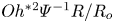 $Oh^{*2} \varPsi ^{-1} R/R_o$: (a) experimental data; (b) the whole set of experimental and numerical data; (c) probability density function (black line) of data in panel (a) around the fitting, compared with a normal distribution with average 0.186 and standard deviation of 9 % (blue dashed line), this distribution is nearly invariant with
  $Oh$; (d) probability density function of data in panel (b) around the fitting. The deviation from an approximate normal (average 0.185, standard deviation 11.1 %) shows a very large deviation on the tails of the distribution.

In contrast, when the whole set of available data is compared with our model, the dispersion around  $Oh^*$ explodes as anticipated in figure 8: this is illustrated in figure 9(b). The statistics of both fittings are also given, noting that the distributions are nearly invariant along the
  $Oh$ range except at the vicinity of
  $Oh^*$. This finding highlights once more the strong sensitivity of the focusing effect on the geometry and the initial conditions: (i) the artificial shape of the initial rim after bursting, which critically determines the initial surface energy content as the pioneering work of Duchemin et al. (Reference Duchemin, Popinet, Josserand and Zaleski2002) revealed; (ii) initial bubble shape; and (iii) the absence or presence of gravity along the evolution. In addition, the numerical accuracy as well as the models for free surface and surface tension reconstruction, etc., also affect the results. Note that the precision of our simulations does not avoid their maximum deviation: the fact that we used an initial edge shape thickness (initial minimum film thickness) equal to 0.1
 $R_o$ and initial hole radius 0.15
 $R_o$, leads to the largest initial meridional radius of curvature among the published initial geometries (see figure 7), which shifts
  $Oh^*$ from 0.03 to 0.034.
In contrast, the actual initial surface energy content after film bursting in real experiments is expected to be fixed by a self-similar process (Eggers & Fontelos Reference Eggers and Fontelos2015, and references therein) with a universal result only in terms of  $Oh$ and
  $Bo$ alone. In effect, despite the relative paucity of data around
  $Oh^*$ and the fact that all the experiments available in this work have been performed with air at atmospheric pressure, naturally including interaction with the gaseous environment, gas compressibility, surface effects (presence of contaminants, surfactants, particles, etc.) and nonlinear breakdown and local detachment of the first droplet, the scatter compared with that of the numerical data is minimal. This supports the general assumption that this problem is fundamentally determined in nature by two non-dimensional parameters only:
  $Oh$ and
  $Bo$.
$Bo$.
On the other hand, the considerably less numerous data available for the ejection velocity  $V$ could be similarly represented in the form
  $\xi ^{1/2} V/V_o$, which tends to
  $V/V_o$ for very small
  $Oh$ and
  $Bo$. However, since our model predicts the ejection velocity at the droplet formation point, while the available data correspond to the ejection velocity measured at a fixed point in space (usually, the initial level of the free surface), a direct comparison with our model predictions is not possible. To compensate for the effect of the different measurement point, which necessarily implies the additional action of viscous dissipation and the work of gravity, we propose a simple velocity correction of the form
 \begin{equation} V/V_o=k_v \varPsi^{{-}1/2} \left(1+ k_1 {Bo} + k_2 {Oh}\right)^{{-}1}, \end{equation}
which, under the same approach as the droplet size approach, provides an optimal fit to the experimental data of (Ghabache et al. Reference Ghabache, Liger-Belair, Antkowiak and Séon2016) for  $k_1=2.27$ and
  $k_2=16$, with a minimum normalized standard deviation below 10 % and a prefactor
  $k_v=0.39$ (see figure 10a). Including the entire data set available for ejection velocity (numerical data from Berny et al. (Reference Berny, Deike, Séon and Popinet2020) and our own), we observe the same drastic increase of the normalized standard deviation for droplet size.
The velocity of the first emitted droplet, expressed as  $\varPsi ^{1/2}(1+ k_1 {Bo} + k_2 {Oh}) V/V_o$, with
  $k_1=2.27$, with
  $k_2=16$, for (a) the experimental data of Ghabache et al. (Reference Ghabache, Liger-Belair, Antkowiak and Séon2016) and Duchemin et al. (Reference Duchemin, Popinet, Josserand and Zaleski2002), after optimal data collapse according to (2.28) and (b) the whole set of available experimental and numerical data, using the same fitting as in panel (a).

3. Concluding statements
Figure 9(a) provides the most robust basis for quantitatively and continuously representing the size of the ejected droplet for the whole range of  $Oh$ and
  $Bo$ where droplet emission occurs. For the convenience of the reader, that universal size can be ultimately written, with typical errors below 10 %, as
 \begin{equation} R=0.18 R_o \bigg(\left(\frac{{Oh}}{{Oh}^*}-1 \right)^2+4.44{Oh}+ 0.19 {Bo}\bigg);\, {Oh}^*=0.03. \end{equation}
 The statistical distribution of experimental data around our model, with an approximately normal distribution and a standard deviation below 10 %, provides solid statistical grounds (i.e. the null hypothesis is virtually excluded) for its consistency and correctness: our model agrees with the available experimental data for the whole  $(Oh, Bo)$ range. We emphasize that (3.1) is not a fitting polynomial expression: it reflexes the physics of the phenomenon as described in this work using just two non-dimensional parameters. The main advantage of (3.1) compared with other proposed models which provide good results but are not valid beyond
  $Oh^*$ (Gañán-Calvo Reference Gañán-Calvo2017, Reference Gañán-Calvo2018; Gordillo & Rodriguez-Rodriguez Reference Gordillo and Rodriguez-Rodriguez2019) is its uniform validity and continuity along the whole
  $(Oh, Bo)$ range. Among an ample variety of applications, this provides a fundamental tool to describe the statistical distribution of the sea spray as a function of the observed bubble size distribution near the sea surface.
A similarly accurate expression for the ejection velocity is not currently possible from available data, due to its strong dependency on the point where it is measured. Based on data at the level of the unperturbed free surface, we propose the following expression from an optimum fitting:
 \begin{align} V= 0.39 V_o
\left(\left({Oh}-{Oh}^*\right)^2+0.004{Oh}+ 0.00017
{Bo}\right)^{{-}1/2} \left(1+ 2.27 {Bo} + 16
{Oh}\right)^{{-}1}. \end{align}
\begin{align} V= 0.39 V_o
\left(\left({Oh}-{Oh}^*\right)^2+0.004{Oh}+ 0.00017
{Bo}\right)^{{-}1/2} \left(1+ 2.27 {Bo} + 16
{Oh}\right)^{{-}1}. \end{align}
Of course, the complexity of the phenomenon can be augmented including surface viscosity (Ponce-Torres et al. Reference Ponce-Torres, Montanero, Herrada, Vega and Vega2017), Marangoni and non-Newtonian effects (Sanjay et al. Reference Sanjay, Lohse and Jalaal2021), the presence of immiscible liquids (Yang, Tian & Thoroddsen Reference Yang, Tian and Thoroddsen2020) or the statistics of the emitted droplets following the first one. In this regard, Berny et al. (Reference Berny, Deike, Séon and Popinet2020) presented a detailed analysis of all issued droplets from the scaling analysis of the first. Despite these are topics of subsequent studies, our results entirely capture the physics needed to describe this phenomenon.
Acknowledgements
B. Gañán-Riesco is thanked for figure 7.
Funding
This research has been supported by the Spanish Ministry of Economy, Industry and Competitiveness (grant numbers DPI2016-78887 and PID2019-108278RB) and by J. de Andalucía (grant number P18-FR-3623).
Declaration of interests
The authors report no conflict of interest.
Author contributions
A.M.G.C. derived the theory, analysed data, reached conclusions and wrote the paper. J.M.L.H. performed the simulations and helped in the writing.


 Open access