


1 Introduction
Flows above concave walls have been studied for over a century due to the strong impact of curvature onto the properties of laminar, turbulent and transitional flows. For instance, curvature affects the stability of boundary layers (Rayleigh Reference Rayleigh1917), the mechanism of transition to turbulence through the occurrence of secondary instabilities (Swearingen & Blackwelder Reference Swearingen and Blackwelder1987), the statistical properties of turbulent boundary layers (Meroney & Bradshaw Reference Meroney and Bradshaw1975) and the decay of anisotropic turbulence in wall-bounded flows (Verschoof et al. Reference Verschoof, Huisman, van der Veen, Sun and Lohse2016; Ostilla-Mónico et al. Reference Ostilla-Mónico, Zhu, Spandan, Verzicco and Lohse2017). The present study describes a relatively simple flow which encompasses laminar, transitional, turbulent and decaying regimes under the influence of concave walls.
Schematic describing the evolution of vorticity (colour coded) and azimuthal velocity profile (vectors) during the distinct stages of the spin-down process: initial condition (ic), laminar stage (I), instabilities and transition to turbulence (II), sustained turbulence with intact vortex core (III), corruption of vortex core and decay of turbulence (IV) and relaminarisation (V). Spirals illustrate the existence of turbulent fluctuations in stages III and IV.

An infinitely long cylinder of radius  $R$ has its axis aligned with the axial direction of a cylindrical coordinate system with radial, azimuthal and axial coordinates denoted respectively ( $r,\unicode[STIX]{x1D711},z$). The cylinder is filled with an incompressible Newtonian fluid of kinematic viscosity $\unicode[STIX]{x1D708}$ and rotated with angular velocity $\unicode[STIX]{x1D6FA}$ (see figure 1) until solid-body rotation (SBR) of constant axial vorticity $\unicode[STIX]{x1D714}=2\unicode[STIX]{x1D6FA}$ is achieved. This flow is characterised by the following velocity field
 $$\begin{eqnarray}u_{\unicode[STIX]{x1D711}}(r)=\unicode[STIX]{x1D6FA}r,\quad u_{r}=u_{z}=0.\end{eqnarray}$$
 The numerical experiment begins at the temporal instant  $t=0$ when, starting from the condition of SBR, the rotation of the cylinder wall is suddenly stopped. Following this event, a transient unsteady flow develops, referred to here as spin-down.
1.1 Motivation and objectives
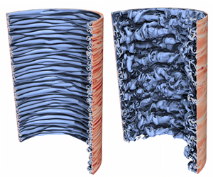
Figure 1 presents the different stages of the spin-down process. Each stage is characterised by unique flow features, which are strongly influenced by the boundary conditions – specifically the concave walls of the cylinder. After the laminar boundary layer formation (stage I), centrifugal instabilities emerge as addressed experimentally by Euteneuer (Reference Euteneuer1972) and Mathis & Neitzel (Reference Mathis and Neitzel1985). These instabilities have also been studied analytically by Neitzel (Reference Neitzel1982) and Kim, Song & Choi (Reference Kim, Song and Choi2008). However, only Euteneuer (Reference Euteneuer1972) extended their work up to the nonlinear saturation of the primary instability (in stage II). Yet the subsequent stages of the spin-down process have not been investigated: the secondary instability (end of stage II), a stage of sustained turbulence (stage III), the decay of turbulence (stage IV) and the relaminarisation (stage V) itself.
These later stages (stages II–V) are characterised by centrifugal instabilities and the onset of turbulence. The kinetic energy initially present in the SBR is not only dissipated through the viscous dissipation associated with a time-varying velocity profile of laminar spin-down, but also converted to turbulent fluctuations and eventually dissipated via turbulent viscous dissipation. When a large fraction of the total energy has been dissipated, turbulence does not self-sustain and a stage of viscous decay occurs yielding relaminarisation. As mentioned in studies on decaying Taylor–Couette (TC) flow by Verschoof et al. (Reference Verschoof, Huisman, van der Veen, Sun and Lohse2016) and Ostilla-Mónico et al. (Reference Ostilla-Mónico, Zhu, Spandan, Verzicco and Lohse2017), the rate at which energy is dissipated during the sustained and decaying turbulent regimes is not known a priori. In a similar manner, the details of production and dissipation of energy associated with turbulent fluctuations are also poorly understood. The statistical properties of the turbulent flow and the turbulence production and decay processes depend on the Reynolds number ( $Re$) in at least two instances. On the one hand, there is the obvious impact of $Re$ on the relative importance of viscous and inertial stresses, and thus on turbulent statistics. On the other hand, the value of $Re$ determines the stability properties of the laminar boundary layer forming at the initial stages of spin-down, thereby determining the boundary-layer properties at the instant in which instability and transition to turbulence occur.
The objective of the present work is to describe the spin-down process throughout all of its phases from onset of centrifugal instabilities to the decay of turbulence. Particular focus lies on the flow stages that have not been discussed previously and on the analysis of the turbulent properties and the effect of  $Re$. This study by no means strives to completely cover all aspects of the spin-down process. Rather the paper provides an initial overview of this complex transient flow and its phenomena. Each stage on its own has significant potential for further investigations and therefore makes the spin-down problem an interesting canonical flow to assess unsteady turbulence in the presence of concave walls.
Each stage of the flow inherits features of related canonical flows influenced by concave wall curvature. As such, the present study attempts to draw parallels to prior studies on concave boundary layers, which are therefore briefly reviewed in the following.
1.2 Review of concave-wall boundary layers
In an axisymmetric two-dimensional flow, the equilibrium between pressure and centrifugal forces is unstable if the magnitude of the circulation  $\unicode[STIX]{x1D6E4}(r)=2\unicode[STIX]{x03C0}\int _{0}^{r}\unicode[STIX]{x1D714}r^{\prime }\,\text{d}r^{\prime }$ ( $\unicode[STIX]{x1D714}$ is the vorticity) decreases with increasing radius $r$. By identifying this inviscid centrifugal instability mechanism Rayleigh (Reference Rayleigh1917) paved the way for research on the influence of curvature on wall-bounded flows. Subsequently, canonical flows with flat boundaries in the streamwise direction
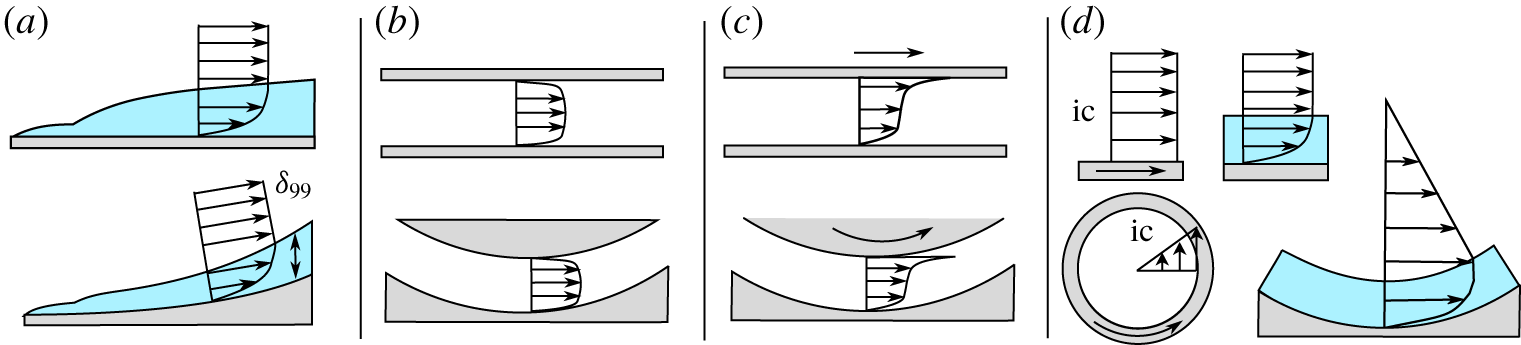
  $s$ were also assessed in their respective curved counterpart (figure 2). Examples include the spatially developing boundary layer (figure 2a, statistically steady, no streamwise pressure gradient $\unicode[STIX]{x2202}p/\unicode[STIX]{x2202}s=0$, spatially developing boundary-layer thickness $\unicode[STIX]{x2202}\unicode[STIX]{x1D6FF}/\unicode[STIX]{x2202}s\neq 0$), the fully developed channel flow (figure 2b, statistically steady, $\unicode[STIX]{x2202}p/\unicode[STIX]{x2202}s\neq 0$, $\unicode[STIX]{x2202}\unicode[STIX]{x1D6FF}/\unicode[STIX]{x2202}s=0$), the Couette flow (figure 2c, statistically steady, $\unicode[STIX]{x2202}p/\unicode[STIX]{x2202}s=0$, $\unicode[STIX]{x2202}\unicode[STIX]{x1D6FF}/\unicode[STIX]{x2202}s=0$) and the temporally developing boundary layer (figure 2d, statistically unsteady, $\unicode[STIX]{x2202}p/\unicode[STIX]{x2202}s=0$, $\unicode[STIX]{x2202}\unicode[STIX]{x1D6FF}/\unicode[STIX]{x2202}s=0$) after a sudden change of boundary conditions. In the following, we briefly review studies that modify these canonical flow scenarios to similar flows over concave walls. As it will become evident later, the present numerical experiment embodies aspects of all such flows.
Overview of distinct boundary-layer types and their concave counterparts: (a) spatially developing boundary layers; (b) fully developed channel flow; (c) Couette and Taylor–Couette flow; (d) temporally developing boundary layers, with the respective initial condition (ic).
Modifying the classic stability problem of a flat, spatially developing boundary layer to account for concave wall curvature (figure 2a) significantly changes its stability properties, as described by Floryan (Reference Floryan1991) and Saric (Reference Saric1994). In flows above concave walls, pairs of streamwise vortices, i.e. Görtler vortices (Görtler Reference Görtler1941), are formed, which get corrupted further downstream by secondary instabilities. Experiments by Bippes (Reference Bippes1972) and Swearingen & Blackwelder (Reference Swearingen and Blackwelder1987) provide visualisations of two distinct secondary instability mechanisms: a sinuous mode, leading to spanwise meandering of the streamwise vortices and a varicose mode, resulting in hairpin-like structures. Linear stability theory was applied to assess the primary instability (Floryan & Saric Reference Floryan and Saric1982) and the secondary instabilities (Hall & Horseman Reference Hall and Horseman1991; Li & Malik Reference Li and Malik1995). Due to its high relevance in turbomachinery, recent work focuses on the receptivity of Görtler vortices towards roughness and free-stream turbulence (Schrader, Brandt & Zaki Reference Schrader, Brandt and Zaki2011; Wu, Zhao & Luo Reference Wu, Zhao and Luo2011), compressibility effects (Ren & Fu Reference Ren and Fu2015) as well as the control of these instabilities (Sescu & Afsar Reference Sescu and Afsar2018).
The canonical, spatially developing boundary layer over flat plates has been extensively studied both in laboratory experiments and in recent numerical simulations (see Schlatter et al. Reference Schlatter, Örlü, Li, Brethouwer, Fransson, Johansson, Alfredsson and Henningson2009; Wu & Moin Reference Wu and Moin2009; Sillero, Jiménez & Moser Reference Sillero, Jiménez and Moser2013). The sizeable computational cost limits the value of  $Re$ that can be achieved in numerical investigations. This limitation is shared also by studies of boundary layers over concave walls, which consist almost exclusively by laboratory experiments. Meroney & Bradshaw (Reference Meroney and Bradshaw1975), Hoffmann, Muck & Bradshaw (Reference Hoffmann, Muck and Bradshaw1985) and Barlow & Johnston (Reference Barlow and Johnston1988) allow transition to turbulence in a straight channel section and, before the flow becomes fully developed, a boundary layer of finite thickness enters a curved section of the channel. The studies revealed persistence of streamwise rolls with wavelengths similar to the boundary-layer thickness even in the turbulent stage, which result in enhanced Reynolds stresses.
Significantly lower computational effort and experimental complexity than in spatially developing boundary layers is required when turbulence is characterised in spatially confined, fully developed and pressure-driven flows such as channels and pipes (see figure 2b and amongst others Kim, Moin & Moser (Reference Kim, Moin and Moser1987)). Experimental (e.g. Hunt & Joubert Reference Hunt and Joubert1979) and numerical (e.g. Moser & Moin Reference Moser and Moin1987) investigations on fully developed curved channel flows also showed deviations in Reynolds stresses due to large-scale, streamwise and wall-parallel vortices with scales similar to the channel height (the so-called Dean instability – Dean (Reference Dean1928)).
Applying curvature to the classical Couette flow leads to a shear flow between two coaxial cylinders: the TC flow, first addressed by Taylor (Reference Taylor1923) (figure 2c). As the system can be easily controlled and is satistically stationary, closed and symmetric, it allows accurate measurements with moderate complexity of the experimental apparatus as well as affordable numerical simulations even for large values of  $Re$. Depending upon the relative and absolute rotational speeds, the radii of the two cylinders and fluid properties, a large variety of different flow structures can be produced. A broad body of literature deals with TC thanks to its simple set-up, the variety of competing physical phenomena occurring in the flow and the similarity with Rayleigh–Bénard convection. Recent reviews are given by Fardin, Perge & Taberlet (Reference Fardin, Perge and Taberlet2014) and Grossmann, Lohse & Sun (Reference Grossmann, Lohse and Sun2016).
The temporal evolution of a turbulent incompressible boundary layer after an impulsive acceleration of a flat wall – the so-called Stokes’ first problem (figure 2d) – is the flat plate counterpart of the problem investigated here in the present study, at least during the first phases of the spin-down process. While the linear stability of the flow was already analysed by Luchini & Bottaro (Reference Luchini and Bottaro2001) almost two decades ago, Kozul, Chung & Monty (Reference Kozul, Chung and Monty2016) recently identified and closed a gap in the literature concerning the in-depth analysis of the turbulent state of such flows. Transferring Stokes’ first problem to a flow with concave wall curvature, results in an azimuthally accelerated cylinder. According to the Rayleigh criterion the effects of centrifugal instabilities are only present in the case of a cylinder deceleration, which corresponds to the spin-down case investigated in the present study. As mentioned above, literature hereby is limited to the early stages of the flow, suggesting that there is merit in further investigations of the subsequent flow stages.
1.3 Outline
The paper is structured as follows. Section 2.1 contains a detailed description of the numerical method and the flow cases considered in the following. Particularly relevant are the description of the adopted Reynolds decomposition and the budget equations utilised to describe the temporal behaviour of the kinetic energy as described in § 2.2, the definition energy spectra (see § 2.4) and the details of the Lagrangian flow visualisation (see § 2.5). Starting with an overview over the temporal flow development in § 3, the different stages of the spin-down are discussed in detail for one of the simulated  $Re$ in §§ 3.1–3.5. Finally, in § 4 the $Re$-influence is addressed by evaluating four simulations at different $Re$, ranging over almost one order of magnitude.
2 Methods
2.1 Numerical procedure
A newly created database of the turbulent spin-down process in cylinders is produced via direct numerical simulation (DNS). The code used in the present study is a mixed-discretisation parallel solver of the incompressible Navier–Stokes equations in cylindrical coordinates (Fabbiane Reference Fabbiane2011; Mascotelli Reference Mascotelli2016). Velocity and pressure fields are discretised via a Fourier–Galerkin approach along the two statistically homogeneous azimuthal ( $\unicode[STIX]{x1D711}$) and axial ( $z$) directions, while second-order explicit compact finite-difference schemes (Lele Reference Lele1992) based on a three-point computational stencil on an inhomogeneous grid are adopted in the radial direction ( $r$). Spectral accuracy is therefore achieved for the discretisation of all differential operators in the statistically homogenous directions. The accuracies of the differential operators $D_{1}=\unicode[STIX]{x2202}/\unicode[STIX]{x2202}r$ and $D^{\ast }=(\unicode[STIX]{x2202}/\unicode[STIX]{x2202}r)(r(\unicode[STIX]{x2202}/\unicode[STIX]{x2202}r))$ operating in the radial direction are fourth and second order, respectively. The incompressibility constraint is enforced within machine accuracy by direct solution of the continuity equation, which is coupled with pressure through the radial component of the momentum equation for the collocation point in the fluid domain closest to the wall. The number of Fourier modes in the azimuthal direction decreases from the wall towards the cylinder axis as a linear function of $r$, so that the azimuthal resolution $r\unicode[STIX]{x1D6E5}\unicode[STIX]{x1D711}$ is kept constant across the cylinder. The regularity boundary conditions (RBC, Lewis & Bellan Reference Lewis and Bellan1990) are based upon the invariance of the solution with respect to the origin of the coordinate system. RBCs are enforced at the cylinder axis, for all wavenumber pairs that exist throughout the cylinder cross-section, or at the radial position that represents the boundary for wavenumber pairs that only exist above certain values of $r$.
$r$.
Discretisation parameters of the direct numerical simulations performed in the present study.  $N_{\unicode[STIX]{x1D711}}^{max}$ and $N_{z}$ are the number of maximum azimuthal and axial Fourier modes used to represent the flow field without accounting for the additional modes required to exactly remove the aliasing error. $N_{r}$ is the number of collocation points adopted in radial direction. The values of spatial and temporal resolutions are computed at the temporal instant of transition to turbulence, for which the friction velocity achieves its maximum value $u_{\unicode[STIX]{x1D70F}}^{max}$. Line colours are used in § 4.

The governing equations are advanced in time starting from the initial condition of a fully established SBR. No pressure gradient is imposed in the axial direction. Temporal discretisation is achieved with an implicit second-order Crank–Nicholson scheme for the linear terms combined with an explicit third-order low-storage Runge–Kutta scheme for the nonlinear part of the governing equations. Random disturbances with constant energy of  $10^{-12}\unicode[STIX]{x1D6FA}^{2}R^{2}$ satisfying no-slip boundary conditions are superimposed to each wavenumber and velocity component of the initial velocity field in the whole cylinder volume. The first time step of the simulation forces the random disturbance to fulfil the continuity equation. In the resulting divergence-free field, the energy contained in each wavenumber and velocity component space is randomly distributed and is bound by $10^{-12.55}\unicode[STIX]{x1D6FA}^{2}R^{2}$ and $10^{-11.5}\unicode[STIX]{x1D6FA}^{2}R^{2}$. Henceforth, governing equations and all variables are normalised via the cylinder radius $R$ and the initial angular velocity $\unicode[STIX]{x1D6FA}$ of the SBR. Four different numerical experiments are performed, characterised by different values of the Reynolds number $Re=\unicode[STIX]{x1D6FA}R^{2}/\unicode[STIX]{x1D708}\in \{3000,6000,12\,000,28\,000\}$, where $\unicode[STIX]{x1D708}$ is the kinematic viscosity of the fluid. The discretisation parameters are summarised in table 1.
Spatial and temporal resolutions are set to fulfil the requirements for wall-bounded turbulence (see Kim et al. Reference Kim, Moin and Moser1987) at all times of the temporal evolution of the flow. The resolutions are expressed in terms of viscous units, i.e. normalised via the kinematic viscosity  $\unicode[STIX]{x1D708}$ of the fluid and the friction velocity $u_{\unicode[STIX]{x1D70F}}=\sqrt{\unicode[STIX]{x1D70F}_{w}/\unicode[STIX]{x1D70C}}$. Here, $\unicode[STIX]{x1D70F}_{w}$ is the spatially averaged wall shear stress and $\unicode[STIX]{x1D70C}$ is the fluid density. Normalisation in viscous units is indicated with the superscript $+$. The most stringent requirement for spatial resolution is achieved after onset of transition, when $u_{\unicode[STIX]{x1D70F}}$ reaches the maximum value $u_{\unicode[STIX]{x1D70F}}^{max}$. At this time instant, indicated by dashed black lines in figure 3(a), the azimuthal, axial and minimum radial resolutions are $R^{+}\unicode[STIX]{x1D6E5}\unicode[STIX]{x1D711}\approx 11$, $\unicode[STIX]{x1D6E5}z^{+}\approx 6$ and $\unicode[STIX]{x1D6E5}r_{min}^{+}\approx 1.5$, respectively. These values are computed without taking into account the additional modes used to exactly remove the aliasing error. It must be noted that such resolution is finer than the one required to correctly describe the onset of turbulent transition, as discussed in § 3. The resolution in viscous units improves for all other later time instants. The axial extent $L_{cyl}$ of the computational domain is a compromise between the need for accommodating several Taylor rolls (Brauckmann & Eckhardt Reference Brauckmann and Eckhardt2013; Ostilla-Mónico et al. Reference Ostilla-Mónico, Stevens, Grossmann, Verzicco and Lohse2013), providing sufficient area for reliable computation of spatially averaged quantities, and constraining the computational effort and the required disk space for storing the large data sets.
(a) Temporal development of the friction velocity  $u_{\unicode[STIX]{x1D70F}}$ at different values of $Re$. The maximum value $u_{\unicode[STIX]{x1D70F}}^{max}$, achieved during transition and used to determine the spatial resolution in the numerical simulation, is marked with dashed black lines. (b) Averaged azimuthal velocity profiles at $\unicode[STIX]{x1D6FA}t=0.5$ (the instant is marked by a vertical dotted orange line in figure 3a) compared with the respective analytical solution (dashed black lines).

2.2 Reynolds decomposition and energy budgets
The spin-down process is statistically unsteady, for which the Reynolds decomposition applied to the velocity field reads
 $$\begin{eqnarray}u_{i}(r,\unicode[STIX]{x1D711},z,t)=\langle u_{i}\rangle _{\unicode[STIX]{x1D711},z}(r,t)+u_{i}^{\prime }(r,\unicode[STIX]{x1D711},z,t),\end{eqnarray}$$
 where index notation is used to indicate the  $i$th velocity component in the respective direction of cylindrical coordinates $(r,\unicode[STIX]{x1D711},z)$; $\langle \cdot \rangle _{\unicode[STIX]{x1D711},z}$ denotes averaging along the statistically homogeneous azimuthal and axial directions. It must be noted that the ensemble average of independent repetitions of the same experiment is applicable to unsteady problems. However, this has not been performed in the present study, for which spatial averaging resulted in sufficient statistical convergence. In equation (2.1), $u_{i}^{\prime }(r,\unicode[STIX]{x1D711},z,t)$ is the fluctuating velocity field about the average value $\langle u_{i}\rangle _{\unicode[STIX]{x1D711},z}(r,t)$. In the following, the notation $\langle u_{i}\rangle =\langle u_{i}\rangle _{\unicode[STIX]{x1D711},z}(r,t)$ and $u_{i}^{\prime }=u_{i}^{\prime }(r,\unicode[STIX]{x1D711},z,t)$ is used for brevity.
The temporal decay of the kinetic energy contained in the initial SBR is investigated in the present study. In the framework of the Reynolds decomposition, kinetic energy is split into mean kinetic energy  $K$, associated with the averaged flow field $\langle u_{i}\rangle$, and turbulent kinetic energy $k$, associated with the fluctuating field $u_{i}^{\prime }$. As $\langle u_{r}\rangle =\langle u_{z}\rangle =0$ in the present flow, the mean kinetic energy is given by $K=1/2\langle u_{\unicode[STIX]{x1D711}}\rangle ^{2}$. Its temporal evolution is governed by the following budget equation:
 $$\begin{eqnarray}\displaystyle \frac{\unicode[STIX]{x2202}K}{\unicode[STIX]{x2202}t} & = & \displaystyle \underbrace{-\frac{\unicode[STIX]{x2202}}{\unicode[STIX]{x2202}r}(\langle u_{\unicode[STIX]{x1D711}}\rangle \langle u_{r}^{\prime }u_{\unicode[STIX]{x1D711}}^{\prime }\rangle )-\frac{\langle u_{\unicode[STIX]{x1D711}}\rangle \langle u_{r}^{\prime }u_{\unicode[STIX]{x1D711}}^{\prime }\rangle }{r}}_{T_{m}}+\underbrace{\frac{\unicode[STIX]{x2202}}{\unicode[STIX]{x2202}r}\left(\unicode[STIX]{x1D708}\langle u_{\unicode[STIX]{x1D711}}\rangle \frac{\unicode[STIX]{x2202}\langle u_{\unicode[STIX]{x1D711}}\rangle }{\unicode[STIX]{x2202}r}\right)+\frac{\unicode[STIX]{x1D708}}{2r}\frac{\unicode[STIX]{x2202}\langle u_{\unicode[STIX]{x1D711}}\rangle ^{2}}{\unicode[STIX]{x2202}r}}_{V_{m}}\cdots \nonumber\\ \displaystyle & & \displaystyle \cdots \underbrace{+\langle u_{r}^{\prime }u_{\unicode[STIX]{x1D711}}^{\prime }\rangle \left(\frac{\unicode[STIX]{x2202}\langle u_{\unicode[STIX]{x1D711}}\rangle }{\unicode[STIX]{x2202}r}-\frac{\langle u_{\unicode[STIX]{x1D711}}\rangle }{r}\right)}_{P}\underbrace{-\unicode[STIX]{x1D708}\left(\frac{\unicode[STIX]{x2202}\langle u_{\unicode[STIX]{x1D711}}\rangle }{\unicode[STIX]{x2202}r}\right)^{2}-\unicode[STIX]{x1D708}\frac{\langle u_{\unicode[STIX]{x1D711}}\rangle ^{2}}{r^{2}}}_{\unicode[STIX]{x1D716}_{m}},\end{eqnarray}$$
 where  $T_{m}$ is the turbulent diffusion, $V_{m}$ the viscous diffusion and $\unicode[STIX]{x1D716}_{m}$ the dissipation of $K$. The turbulence production term $P$ couples the budget equation of $K$ and $k$ as it draws energy from the mean flow and transfers it to the fluctuating field. Following Mansour, Kim & Moin (Reference Mansour, Kim and Moin1988) and Bilson & Bremhorst (Reference Bilson and Bremhorst2007) the budget equation for $k=(1/2)(\langle u_{z}^{\prime }u_{z}^{\prime }\rangle +\langle u_{r}^{\prime }u_{r}^{\prime }\rangle +\langle u_{\unicode[STIX]{x1D711}}^{\prime }u_{\unicode[STIX]{x1D711}}^{\prime }\rangle )$ is given by
 $$\begin{eqnarray}\displaystyle \frac{\unicode[STIX]{x2202}k}{\unicode[STIX]{x2202}t} & = & \displaystyle \underbrace{-\frac{1}{2r}\frac{\unicode[STIX]{x2202}(r\langle u_{r}^{\prime }u_{i}^{\prime }u_{i}^{\prime }\rangle )}{\unicode[STIX]{x2202}r}}_{T_{t}}+\underbrace{\frac{\unicode[STIX]{x1D708}}{2r}\frac{\unicode[STIX]{x2202}}{\unicode[STIX]{x2202}r}\left(r\frac{\unicode[STIX]{x2202}\overline{(u_{i}^{\prime }u_{i}^{\prime })}}{\unicode[STIX]{x2202}r}\right)}_{V_{t}}\cdots \nonumber\\ \displaystyle & & \displaystyle \cdots \underbrace{-\frac{1}{\unicode[STIX]{x1D70C}}\left(\frac{\unicode[STIX]{x2202}(\langle u_{r}^{\prime }p^{\prime }\rangle )}{\unicode[STIX]{x2202}r}+\frac{\langle u_{r}^{\prime }p^{\prime }\rangle }{r}\right)}_{\unicode[STIX]{x1D6F1}^{d}}\underbrace{-\langle u_{r}^{\prime }u_{\unicode[STIX]{x1D711}}^{\prime }\rangle \left(\frac{\unicode[STIX]{x2202}\langle u_{\unicode[STIX]{x1D711}}\rangle }{\unicode[STIX]{x2202}r}-\frac{\langle u_{\unicode[STIX]{x1D711}}\rangle }{r}\right)}_{P}\cdots \nonumber\\ \displaystyle & & \displaystyle \cdots -\underbrace{\unicode[STIX]{x1D708}\left[\left\langle \frac{\unicode[STIX]{x2202}u_{i}^{\prime }}{\unicode[STIX]{x2202}z}\frac{\unicode[STIX]{x2202}u_{i}^{\prime }}{\unicode[STIX]{x2202}z}\right\rangle +\left\langle \frac{\unicode[STIX]{x2202}u_{i}^{\prime }}{\unicode[STIX]{x2202}r}\frac{\unicode[STIX]{x2202}u_{i}^{\prime }}{\unicode[STIX]{x2202}r}\right\rangle +\frac{1}{r^{2}}\left\langle \left(\frac{\unicode[STIX]{x2202}u_{\unicode[STIX]{x1D711}}^{\prime }}{\unicode[STIX]{x2202}\unicode[STIX]{x1D711}}+u_{r}^{\prime }\right)^{2}+\left(\frac{\unicode[STIX]{x2202}u_{r}^{\prime }}{\unicode[STIX]{x2202}\unicode[STIX]{x1D711}}-u_{\unicode[STIX]{x1D711}}^{\prime }\right)^{2}\right\rangle \right]}_{\unicode[STIX]{x1D716}_{t}}.\nonumber\\ \displaystyle & & \displaystyle\end{eqnarray}$$
 Here, the viscous diffusion  $V_{t}$, the pressure diffusion $\unicode[STIX]{x1D6F1}^{d}$ and the turbulent diffusion $T_{t}$ describe the transport of $k$, while $\unicode[STIX]{x1D716}_{t}$ is its viscous dissipation.
Beyond the averaging in the axial and azimuthal directions, the closed system allows averaging in the cylinder volume  $V$, which is indicated in the following with the volume averaging operator $[\cdot ]$. The volume-averaged total kinetic energy $[K]+[k]$ can be expressed as
 $$\begin{eqnarray}[K]+[k]=\frac{1}{2V\unicode[STIX]{x1D6FA}^{2}R^{2}}\int _{V}u_{i}u_{i}\,\text{d}V=\frac{1}{2V\unicode[STIX]{x1D6FA}^{2}R^{2}}\int _{V}\langle u_{i}\rangle ^{2}\,\text{d}V+\frac{1}{2V\unicode[STIX]{x1D6FA}^{2}R^{2}}\int _{V}\langle u_{i}^{\prime }u_{i}^{\prime }\rangle \,\text{d}V.\end{eqnarray}$$
 Due to the no-slip conditions at the decelerated cylinder walls, energy is constantly withdrawn from the system. The temporal change of kinetic energy  $[K]+[k]$ can be described by volume averaging and summation of the equations (2.2) and (2.3). All transport terms $T_{t}$, $V_{t}$, $T_{m}$, $V_{m}$ and $\unicode[STIX]{x1D6F1}_{d}$ contained in the two equations vanish by definition. Also the production $P$, which appears in both equations for $[K]$ and $[k]$ with an opposite sign, vanishes when the volume average of the kinetic energy $[K]+[k]$ is evaluated. As a consequence, only the dissipation terms $\unicode[STIX]{x1D716}_{t}$ and $\unicode[STIX]{x1D716}_{m}$ remain
 $$\begin{eqnarray}\frac{\unicode[STIX]{x2202}([K]+[k])}{\unicode[STIX]{x2202}t}=\frac{\unicode[STIX]{x2202}[K]}{\unicode[STIX]{x2202}t}+\frac{\unicode[STIX]{x2202}[k]}{\unicode[STIX]{x2202}t}=[\unicode[STIX]{x1D716}_{m}]+[\unicode[STIX]{x1D716}_{t}]=[\unicode[STIX]{x1D716}_{tot}].\end{eqnarray}$$
2.3 Wall-based flow description
To characterise turbulence in the developing boundary layer during spin-down, the classical friction Reynolds number
 $$\begin{eqnarray}Re_{\unicode[STIX]{x1D70F}}=u_{\unicode[STIX]{x1D70F}}\unicode[STIX]{x1D6FF}_{99}/\unicode[STIX]{x1D708}\end{eqnarray}$$
 is introduced (Jiménez et al. Reference Jiménez, Hoyas, Simens and Mizuno2010), in which  $\unicode[STIX]{x1D6FF}_{99}$ is the boundary-layer thickness and $u_{\unicode[STIX]{x1D70F}}=\sqrt{\unicode[STIX]{x1D70F}_{w}/\unicode[STIX]{x1D70C}}$ is the friction velocity based on the mean wall shear stress
 $$\begin{eqnarray}\left.\unicode[STIX]{x1D70F}_{w}=\unicode[STIX]{x1D70C}\unicode[STIX]{x1D708}\frac{\unicode[STIX]{x2202}\langle u_{\unicode[STIX]{x1D711}}\rangle }{\unicode[STIX]{x2202}r}\right|_{r=R}.\end{eqnarray}$$
 Note that in the investigated flow  $\unicode[STIX]{x1D70F}_{w}$, $u_{\unicode[STIX]{x1D70F}}$, $\unicode[STIX]{x1D6FF}_{99}$ and $Re_{\unicode[STIX]{x1D70F}}$ change with time $t$. Due to the lack of a constant outer velocity, the traditional definition of $\unicode[STIX]{x1D6FF}_{99}$ is adapted by using the retracting vortex core in SBR as follows
 $$\begin{eqnarray}\unicode[STIX]{x1D6FA}(R-\unicode[STIX]{x1D6FF}_{99})-\langle u_{\unicode[STIX]{x1D711}}\rangle =0.01\unicode[STIX]{x1D6FA}R,\end{eqnarray}$$
 i.e.  $\unicode[STIX]{x1D6FF}_{99}$ is defined as the distance from the wall, at which the flow deviates $0.01\unicode[STIX]{x1D6FA}R$ from the initial SBR.
2.4 Energy spectra
The appearance of Taylor–Görtler rolls will be assessed by the analysis of the power spectral density of  $k$. The summands of $k=1/2\langle u_{i}^{\prime }u_{i}^{\prime }\rangle$ are split up into the contribution of different axial modes $\unicode[STIX]{x1D705}_{z}$ of wavelength $\unicode[STIX]{x1D706}_{z}=L_{cyl}/\unicode[STIX]{x1D705}_{z}$. The axial energy spectra are given by
 $$\begin{eqnarray}\unicode[STIX]{x1D6F7}_{u_{i}u_{i}}=\unicode[STIX]{x1D6F7}_{u_{i}u_{i}}(r,\unicode[STIX]{x1D705}_{z})=\int _{\unicode[STIX]{x1D705}_{\unicode[STIX]{x1D711}}^{min}}^{\unicode[STIX]{x1D705}_{\unicode[STIX]{x1D711}}^{max}}\mathfrak{R}\langle \hat{u} _{i}(\unicode[STIX]{x1D705}_{\unicode[STIX]{x1D711}},\unicode[STIX]{x1D705}_{z},r)\hat{u} _{i}^{\ast }(\unicode[STIX]{x1D705}_{\unicode[STIX]{x1D711}},\unicode[STIX]{x1D705}_{z},r)\rangle \,\text{d}\unicode[STIX]{x1D705}_{\unicode[STIX]{x1D711}},\end{eqnarray}$$
 where  $\mathfrak{R}$ is the real part of a complex number, $\hat{\cdot }$ indicates the Fourier coefficients and the superscript $\ast$ denotes complex conjugation. By accumulating the energy of all modes except the base flow the summands of $k$ are recovered,
 $$\begin{eqnarray}\langle u_{i}^{\prime }u_{i}^{\prime }\rangle (r,t)=\int _{\unicode[STIX]{x1D705}_{z}^{1}}^{\unicode[STIX]{x1D705}_{z}^{max}}\unicode[STIX]{x1D6F7}_{u_{i}u_{i}}\,\text{d}\unicode[STIX]{x1D705}_{z}=\int _{\unicode[STIX]{x1D706}_{z}^{min}}^{\unicode[STIX]{x1D706}_{z}^{max}}\unicode[STIX]{x1D705}_{z}\unicode[STIX]{x1D6F7}_{u_{i}u_{i}}\,\text{d}(\text{ln}(\unicode[STIX]{x1D706}_{z})).\end{eqnarray}$$
 To gather information about the linear and subsequent nonlinear growth of the different modes  $\unicode[STIX]{x1D705}_{z}$ in the boundary layer, the energy spectrum $\unicode[STIX]{x1D6F7}_{u_{\unicode[STIX]{x1D711}}u_{\unicode[STIX]{x1D711}}}$ is spatially averaged over the fluid volume contained in the boundary layer $V_{\unicode[STIX]{x1D6FF}}=\unicode[STIX]{x03C0}(2R\unicode[STIX]{x1D6FF}_{99}-\unicode[STIX]{x1D6FF}_{99}^{2})L_{cyl}$, resulting in the one-dimensional (1-D) spectrum
 $$\begin{eqnarray}\frac{1}{V_{\unicode[STIX]{x1D6FF}}}\int _{V_{\unicode[STIX]{x1D6FF}}}\int _{\unicode[STIX]{x1D705}_{z}^{1}}^{\unicode[STIX]{x1D705}_{z}^{max}}\unicode[STIX]{x1D6F7}_{u_{\unicode[STIX]{x1D711}}u_{\unicode[STIX]{x1D711}}}\,\text{d}\unicode[STIX]{x1D705}_{z}\,\text{d}V=\int _{\unicode[STIX]{x1D705}_{z}^{1}}^{\unicode[STIX]{x1D705}_{z}^{max}}\underbrace{\frac{2\unicode[STIX]{x03C0}L_{cyl}}{V_{\unicode[STIX]{x1D6FF}}}\int _{R-\unicode[STIX]{x1D6FF}_{99}}^{R}\unicode[STIX]{x1D6F7}_{u_{\unicode[STIX]{x1D711}}u_{\unicode[STIX]{x1D711}}}r\,\text{d}r}_{\unicode[STIX]{x1D709}_{\unicode[STIX]{x1D711}\unicode[STIX]{x1D711}}(\unicode[STIX]{x1D705}_{z})}\,\text{d}\unicode[STIX]{x1D705}_{z}\end{eqnarray}$$
 for each time step;  $\unicode[STIX]{x1D709}_{\unicode[STIX]{x1D711}\unicode[STIX]{x1D711}}$ thus describes the contribution to $\langle u_{\unicode[STIX]{x1D711}}^{\prime }u_{\unicode[STIX]{x1D711}}^{\prime }\rangle$ of each wavenumber $\unicode[STIX]{x1D705}_{z}$ throughout the whole boundary layer.
2.5 Lagrangian flow visualisation: finite-time Lyapunov exponent
The identification of Lagrangian coherent structures (LCS) can provide deeper insight into the material transport of complex flows (Haller Reference Haller2015). LCS separate flow regions of coherent movement. A classical method to calculate attracting LCS is the backward finite-time Lyapunov exponent (FTLE)  $\unicode[STIX]{x1D70E}_{T_{int}}^{b}(t)$, which determines the local attraction rate of particle tracks over a finite time span. The first step to determine the backward FTLE is seeding massless tracers in the computational domain and tracking them backward in time over the timespan $T_{int}$. In the present work, flow-map interpolation as suggested by Brunton & Rowley (Reference Brunton and Rowley2010) is applied to reduce the computational effort. The resulting flow map $\unicode[STIX]{x1D6F9}_{t}^{t-T_{int}}$ is used to determine the right Cauchy–Green tensor
 $$\begin{eqnarray}C=(\unicode[STIX]{x1D735}\unicode[STIX]{x1D6F9}_{t}^{t-T^{int}})^{\text{T}}\unicode[STIX]{x1D735}\unicode[STIX]{x1D6F9}_{t}^{t-T_{int}}.\end{eqnarray}$$
 The terms of the deformation gradient  $\unicode[STIX]{x1D735}\unicode[STIX]{x1D6F9}_{t}^{t-T_{int}}$ are obtained by the numerical schemes described in § 2.1. By evaluating and normalising the maximum eigenvalue $\unicode[STIX]{x1D6EC}_{max}(C)$, the backward FTLE
 $$\begin{eqnarray}\unicode[STIX]{x1D70E}_{T_{int}}^{b}(t)=\frac{1}{T_{int}}\text{ln}(\unicode[STIX]{x1D6EC}_{max}(C))\end{eqnarray}$$
is determined. Shadden, Lekien & Marsden (Reference Shadden, Lekien and Marsden2005) define thin ridges of the FTLE as LCS. For the present flow, the FTLE provides a clear visualisation of the complex three-dimensional interface between the boundary layer and the vortex core. The FTLE is particularly useful during the onset of three-dimensionality in the flow, as it captures the location and evolution of the secondary instability through an alternative visualisation of the flow field.
3 Flow stages
Dimensional analysis provides two dimensionless groups for the present flow: the Reynolds number  $Re=\unicode[STIX]{x1D6FA}R^{2}/\unicode[STIX]{x1D708}$ and a dimensionless time. Two distinct yet convertible representations of the dimensionless time are utilised in the following: the viscous time $\unicode[STIX]{x1D708}t/R^{2}$ and the outer time $\unicode[STIX]{x1D6FA}t=Re\cdot \unicode[STIX]{x1D708}t/R^{2}$, where $\unicode[STIX]{x1D6FA}t=2\unicode[STIX]{x03C0}$ represents a full revolution of the SBR. This section discusses the temporal development of the spin-down flow at $Re=12\,000$, before the $Re$ scaling is addressed in § 4.
Temporal development of bulk flow statistics for the spin-down process at $Re=12\,000$: (a) boundary-layer thickness $\unicode[STIX]{x1D6FF}_{99}$, friction velocity $u_{\unicode[STIX]{x1D70F}}$ and friction Reynolds number $Re_{\unicode[STIX]{x1D70F}}$; (b) mean $[K]$ and turbulent $[k]$ kinetic energy. Roman numbers I–V and background colouring indicate the different stages of the decay process.

Temporal development of the volume-averaged  $[K]$ (2.2) and $[k]$ (2.3) budgets for the spin-down flow at $Re=12\,000$: (a) turbulent production $[P]$, mean dissipation $[\unicode[STIX]{x1D716}_{m}]$, turbulent dissipation $[\unicode[STIX]{x1D716}_{t}]$ and total dissipation $[\unicode[STIX]{x1D716}_{tot}]$; (b) ratio $[\unicode[STIX]{x1D716}_{t}]/[\unicode[STIX]{x1D716}_{m}]$ and excess production $|[P]/[\unicode[STIX]{x1D716}_{t}]|$.

Figures 4 and 5 provide a first overview of the flow evolution. Roman numbers I–V and background colouring indicate the different stages of the decay process. While each stage is characterised by unique features, the transition between stages occurs gradually and thus cannot be exactly localised in time.
During stage I, a stable, laminar boundary layer grows from the cylinder wall at a rate proportional to the viscous time scale  $\sqrt{\unicode[STIX]{x1D708}t}$ (see figure 4a), while the friction velocity $u_{\unicode[STIX]{x1D70F}}$ decreases. Since the increase in boundary-layer thickness outweighs the decrease in $u_{\unicode[STIX]{x1D70F}}$, $Re_{\unicode[STIX]{x1D70F}}$ increases mildly in time. Figure 4(b) shows the corresponding evolution of volume-averaged mean and turbulent kinetic energy. As expected, $[K]$ decreases and the initial random disturbances contained in $[k]$ also decay in the stable boundary layer. Stage II is characterised by the centrifugal instability associated with the emergence of Taylor vortices and subsequent breakdown to turbulence. The sudden increase of $u_{\unicode[STIX]{x1D70F}}$ and $\unicode[STIX]{x1D6FF}_{99}$ (and thus $Re_{\unicode[STIX]{x1D70F}}$) is accompanied by the exponential growth of $[k]$.
After transition to turbulence, stage III is entered. In this stage,  $[k]$ varies slowly in time. The flow consists of the superposition of a constantly retracting SBR core at the centre of the cylinder and a turbulent boundary layer close to the cylinder wall. The latter is characterised by decreasing $u_{\unicode[STIX]{x1D70F}}$ and increasing $\unicode[STIX]{x1D6FF}_{99}$. The beginning of stage IV is marked by the breakdown of the SBR core, in which turbulent fluctuations become non-negligible and induce a reduction of $\langle u_{\unicode[STIX]{x1D711}}\rangle$ inside the vortex core. Two distinct phenomena occur during stage IV. First, the breakdown of the SBR core is accompanied by a sudden increase of $\unicode[STIX]{x1D6FF}_{99}$ with no discernible effect on $u_{\unicode[STIX]{x1D70F}}$ or $[k]$. Then, after the SBR core has been completely eroded by turbulence, $[k]$ and $Re_{\unicode[STIX]{x1D70F}}$ drop in time. Finally, the temporal evolution of the flow ends with the viscous decay of stage V.
Figure 5(a) shows the temporal evolution of  $[P]$, $[\unicode[STIX]{x1D716}_{t}]$ and $[\unicode[STIX]{x1D716}_{m}]$ during the five stages. In stage I, energy dissipation is governed by $[\unicode[STIX]{x1D716}_{m}]$, while very small values of $[\unicode[STIX]{x1D716}_{t}]$ indicate the decay of the initial disturbances (figure 5a). At the end of stage I, $[P]$ begins to increase in time until $[P]$ exceeds $[\unicode[STIX]{x1D716}_{t}]$, at which point the Taylor rolls emerge in stage II and yield the fast increase of $[k]$ discussed above. The onset of turbulence is accompanied by a strong increase of $[\unicode[STIX]{x1D716}_{t}]/[\unicode[STIX]{x1D716}_{m}]$ (figure 5b), after which $[\unicode[STIX]{x1D716}_{t}]$ and $[P]$ are in equilibrium, yielding the sustained turbulent regime of stage III with only marginal variation of $[k]$ (figure 4b). Within stage IV the ratio of dissipation $[\unicode[STIX]{x1D716}_{t}]$ and production $[P]$ leans towards dissipation and $[k]$ begins to decay. Eventually, the flow laminarises and the ratio $[\unicode[STIX]{x1D716}_{t}]/[\unicode[STIX]{x1D716}_{m}]$ drops significantly while $[\unicode[STIX]{x1D716}_{tot}]\approx [\unicode[STIX]{x1D716}_{m}]$. This final stage, which is most evident in figure 5(b), is referred to as stage V.
3.1 Stage I: laminar boundary layer
The laminar stage of the flow, for which  $u_{i}^{\prime }=0$ and thus $u_{\unicode[STIX]{x1D711}}^{lam}=\langle u_{\unicode[STIX]{x1D711}}\rangle$, can be described by the analytical solution of Neitzel (Reference Neitzel1982)
 $$\begin{eqnarray}\frac{u_{\unicode[STIX]{x1D711}}^{lam}}{\unicode[STIX]{x1D6FA}R}=-2\mathop{\sum }_{i=1}^{\infty }\frac{\text{J}_{1}(\unicode[STIX]{x1D6FD}_{i}r/R)}{\unicode[STIX]{x1D6FD}_{i}\text{J}_{0}(\unicode[STIX]{x1D6FD}_{i})}\text{exp}(-\unicode[STIX]{x1D6FD}_{i}^{2}\unicode[STIX]{x1D708}t/R^{2}),\end{eqnarray}$$
 where  $\text{J}_{0}$ and $\text{J}_{1}$ are Bessel functions of the first kind and $\unicode[STIX]{x1D6FD}_{i}$ are roots of $\text{J}_{1}(\unicode[STIX]{x1D6FD}_{i})=0$. For small $t$, while $\unicode[STIX]{x1D6FF}_{99}/R$ is small and the local curvature is negligible, the present boundary layer above the concave wall is similar to Stokes’ first problem (e.g. Schlichting Reference Schlichting1979). Thus, for small $t$, the growth rate of $\unicode[STIX]{x1D6FF}_{99}$ coincides with the growth rate of the boundary layer in the vicinity of a impulsively accelerated flat plate (here indicated with the superscript $St$),
 $$\begin{eqnarray}\unicode[STIX]{x1D6FF}_{99}^{St}=a_{lam}^{St}\sqrt{\unicode[STIX]{x1D708}t}\approx 3.64\sqrt{\unicode[STIX]{x1D708}t}.\end{eqnarray}$$
 However, with increasing  $\unicode[STIX]{x1D6FF}_{99}/R$ the growth rate of $\unicode[STIX]{x1D6FF}_{99}$ in the spin-down problem, computed exploiting the exact analytical solution (3.1), deviates from $\unicode[STIX]{x1D6FF}_{99}^{St}$ due to curvature effects. The deviation is such that $\unicode[STIX]{x1D6FF}_{99}$ can be made directly proportional to $\sqrt{\unicode[STIX]{x1D708}t}$, only if the proportionality coefficient $a_{lam}$ is a weak function of time.
For simplicity, in the following analyses the growth rate during stage I is characterised through a constant growth rate coefficient  $a_{lam}$, which is determined via a least square fit of the expression
 $$\begin{eqnarray}\unicode[STIX]{x1D6FF}_{99}\approx a_{lam}\sqrt{\unicode[STIX]{x1D708}t}\end{eqnarray}$$
 to the analytical solution for the spin-down process, which yields  $a_{lam}\approx 3.68$. The approximation of neglecting the temporal variation of $a_{lam}$ in (3.3) introduces an error smaller than $0.01\unicode[STIX]{x1D6FF}_{99}$ for $0<\unicode[STIX]{x1D6FF}_{99}<0.28R$. The good agreement of (3.3) (black line) with the numerical results is emphasised in figures 4(a) and 7(a).
(a) Critical wavelength  $\unicode[STIX]{x1D706}_{c}$ as a function of $Re$. Hollow symbols and lines are experimental data and correlations from the literature mentioned in the legend, respectively. Green dots denote current results. Note that the values of $\unicode[STIX]{x1D706}_{c}$ reported by Maxworthy (Reference Maxworthy, Paterson and Zakin1971) and Mathis & Neitzel (Reference Mathis and Neitzel1985) have been rescaled by a factor 0.5 due to their different definition of $\unicode[STIX]{x1D706}_{c}$, as noted by Kim & Choi (Reference Kim and Choi2006). (b) Temporal evolution of $\unicode[STIX]{x1D6FF}_{99}$ and $\unicode[STIX]{x1D706}_{T}(t)$ for the present numerical simulation compared against the measurement by Euteneuer (Reference Euteneuer1972) at $Re=12\,000$.

3.2 Stage II: emergence of Taylor rolls and laminar-to-turbulent transition
If  $Re$ is large enough (the stability limit in the literature varies in the range of $128<Re<350$), the boundary layer is linearly stable only until a critical time $\unicode[STIX]{x1D703}_{c}=\unicode[STIX]{x1D708}t_{c}/R^{2}$, after which the boundary layer undergoes linear primary centrifugal instability. The instability results in the emergence of radial plumes, which later evolve into Taylor rolls. The plumes occur at a characteristic time-dependent spacing $\unicode[STIX]{x1D706}_{T}(t)$ in the axial direction, which at the critical time $\unicode[STIX]{x1D703}_{c}$ is representative of the linearly most-amplified axial wavelength, the so-called critical wavelength $\unicode[STIX]{x1D706}_{c}=\unicode[STIX]{x1D706}_{T}(\unicode[STIX]{x1D703}_{c})$. For the sake of validation, the values of $\unicode[STIX]{x1D706}_{c}$ extracted from the present numerical simulation are compared in figure 6(a) against results obtained in the literature via linear stability analyses (i.e. Kim & Choi Reference Kim and Choi2006) and laboratory experiments (Maxworthy Reference Maxworthy, Paterson and Zakin1971; Euteneuer Reference Euteneuer1969, Reference Euteneuer1972; Mathis & Neitzel Reference Mathis and Neitzel1985). In the present work, $\unicode[STIX]{x1D706}_{c}$ is measured as the most energetic wavelength of $\unicode[STIX]{x1D709}_{\unicode[STIX]{x1D711}\unicode[STIX]{x1D711}}(\unicode[STIX]{x1D705}_{z},\unicode[STIX]{x1D703}_{c})$ (see § 2.4 for the definition of $\unicode[STIX]{x1D709}_{\unicode[STIX]{x1D711}\unicode[STIX]{x1D711}}$) during the early stage of the linear growth and shows excellent agreement with these existing studies.
Temporal history of  $\unicode[STIX]{x1D6FF}_{99}$ and $u_{\unicode[STIX]{x1D70F}}$ in (a); $[K]$ and $[k]$ in (b); $\unicode[STIX]{x1D709}_{\unicode[STIX]{x1D711}\unicode[STIX]{x1D711}}(\unicode[STIX]{x1D705}_{z},t)$ in (c,d) for the spin-down flow at $Re=12\,000$. The wavenumber and temporal dependence of $\unicode[STIX]{x1D709}_{\unicode[STIX]{x1D711}\unicode[STIX]{x1D711}}(\unicode[STIX]{x1D705}_{z},t)$ are colour-coded in (c) and (d) respectively. The vertical dashed lines indicate the four temporal instances $\unicode[STIX]{x1D6FA}t\in \{1.0,2.0,4.3,5.3\}$ that are discussed in detail in figure 8. The vertical dotted line marks the onset of turbulence as visualised in figure 10(a). The vertical dashed-dotted line in (d) marks the critical wavenumber $\unicode[STIX]{x1D705}_{c}$.

Figure 6(b) compares  $\unicode[STIX]{x1D706}_{T}(t)$ computed from the present numerical data against the experimental results of Euteneuer (Reference Euteneuer1972) at $Re=12\,000$. Euteneuer (Reference Euteneuer1972) estimated the critical wavelength by counting the number of toroidal Taylor rolls aligned along the axial dimension of his experimental set-up. It was found that the rate of change in the observed number of streamwise rolls changes abruptly. This change in growth rate was referred to as ‘Knickstelle’, the German word for ‘kink’, the origin of which will be discussed in the following.
Figure 7 shows the initial evolution of  $\unicode[STIX]{x1D6FF}_{99}$, $u_{\unicode[STIX]{x1D70F}}$, $[k]$, $[K]$ and $\unicode[STIX]{x1D709}_{\unicode[STIX]{x1D711}\unicode[STIX]{x1D711}}$. The flow at four selected time instances, marked with dashed black lines in figure 7, is visualised in figure 8. Figure 8 consists of a pre-multiplied spectrum $\unicode[STIX]{x1D705}_{z}\unicode[STIX]{x1D6F7}_{u_{i}u_{i}}$, the 1-D spectrum $\unicode[STIX]{x1D709}_{\unicode[STIX]{x1D711}\unicode[STIX]{x1D711}}$ averaged over the boundary layer and a $(r,z)$-slice of $u_{\unicode[STIX]{x1D711}}^{\prime }$. The respective boundary-layer thickness $\unicode[STIX]{x1D6FF}_{99}$ is depicted with an orange line. The complete corresponding temporal evolution is provided in supplementary material Movie1.mp4 available at https://doi.org/10.1017/jfm.2019.974.
Pre-multiplied 1-D spectra  $\unicode[STIX]{x1D705}_{z}\unicode[STIX]{x1D6F7}_{u_{i}u_{i}}$ (left), 1-D spectra $\unicode[STIX]{x1D709}_{\unicode[STIX]{x1D711}\unicode[STIX]{x1D711}}$ averaged across the boundary layer (middle) and instantaneous velocity fluctuations $u_{\unicode[STIX]{x1D711}}^{\prime }$ (right) during transition ( $Re=12\,000$). The orange line marks the boundary-layer thickness $\unicode[STIX]{x1D6FF}_{99}$ (left and right) and the wavenumber $\unicode[STIX]{x1D705}_{\unicode[STIX]{x1D6FF}}=2\times 2\unicode[STIX]{x03C0}/\unicode[STIX]{x1D6FF}_{99}$, which would be the most energetic wavenumber if the streamwise vortices were circular and had diameter $\unicode[STIX]{x1D6FF}_{99}$. The vertical dashed-dotted line marks the critical wavelength $\unicode[STIX]{x1D706}_{c}$ (left) and wavenumber $\unicode[STIX]{x1D705}_{c}$ (right), respectively. (a) Exponential growth of primary instability: $\unicode[STIX]{x1D6FA}t=1$. (b) Exponential growth for a broad range of modes: $\unicode[STIX]{x1D6FA}t=2$. (c) Significant influence of instabilities onto the mean flow: $\unicode[STIX]{x1D6FA}t=4.3$. (d) Right before onset of secondary instability: $\unicode[STIX]{x1D6FA}t=5.3$.

During the early linear stage ( $\unicode[STIX]{x1D6FA}t=1$, figure 8a) most modes decay and only a narrow band of axial wavenumbers $\unicode[STIX]{x1D705}_{z}\approx \unicode[STIX]{x1D705}_{c}$ is amplified. This is most clearly visible in figure 7(c), where the temporal evolution of $\unicode[STIX]{x1D709}_{\unicode[STIX]{x1D711}\unicode[STIX]{x1D711}}$ is reported for relevant wavenumbers. As the mean velocity profile changes due to the temporal growth of the boundary layer, the stability properties of the mean velocity profile also change, and so does the most amplified wavenumber. Already at $\unicode[STIX]{x1D6FA}t=2$ wavenumbers $\unicode[STIX]{x1D705}_{z}<\unicode[STIX]{x1D705}_{c}$ are amplified and carry more energy than $\unicode[STIX]{x1D705}_{c}$. This temporal change of the most amplified disturbances are represented in figure 7(d), in which $\unicode[STIX]{x1D709}_{\unicode[STIX]{x1D711}\unicode[STIX]{x1D711}}$ is reported as function of $\unicode[STIX]{x1D705}_{z}$ at different temporal instances distinguishable through colour coding from the start of spin-down (bright colour) onwards.
Starting from  $\unicode[STIX]{x1D6FA}t=2$ the energy of almost all wavenumbers grows exponentially, leading to increasing $[k]$ (figure 7b), until nonlinear saturation is reached and the growth stops at $\unicode[STIX]{x1D6FA}t=4.3$. At this moment, the initially amplified wavenumbers achieve their maximum energy content. The fluctuations start to influence the mean profile $\langle u_{\unicode[STIX]{x1D711}}\rangle$ and thus $\unicode[STIX]{x1D6FF}_{99}$, $u_{\unicode[STIX]{x1D70F}}$ and $[K]$. The pre-multiplied spectrum $\unicode[STIX]{x1D6F7}_{u_{z}u_{z}}$ shows a distinct second peak at a radial position close to $\unicode[STIX]{x1D6FF}_{99}$, marked by an orange line in the left panels of figures 8(c) and 8(d). The second peak is related to the axial flow at the head of the radial jets, which starts the formation of plumes and streamwise vortices by redirecting the radial flow in axial direction. This process is accompanied by a simultaneous rapid growth of $\unicode[STIX]{x1D6FF}_{99}$, $u_{\unicode[STIX]{x1D70F}}$ and $[k]$ (figures 7a and 7b).
FTLE visualisations of the transition process to turbulence at  $Re=12\,000$: (a) $\unicode[STIX]{x1D6FA}t=4.3$, primary instability; (b) $\unicode[STIX]{x1D6FA}t=4.8$, asymmetric growth of primary instability; (c) $\unicode[STIX]{x1D6FA}t=5.3$, observable streamwise ends of streamwise vortices; (d) $\unicode[STIX]{x1D6FA}t=5.8$, onset hairpin-like vortices; (e) $\unicode[STIX]{x1D6FA}t=6.8$, corruption of streamwise vortices; (f) $\unicode[STIX]{x1D6FA}t=7.8$, late transition.

The friction velocity  $u_{\unicode[STIX]{x1D70F}}$ reaches its maximum at $\unicode[STIX]{x1D6FA}t=5.3$, right before the breakdown of this still coherent and quasi-axisymmetric flow through presence of a secondary instability. This effect will be discussed later in more detail. At this instance (figure 9e), the plumes are roughly twice as tall in the radial direction than they are wide in the axial direction, and begin to merge with adjacent plumes towards restoring an aspect ratio of unity. The sudden merging of consecutive plumes causes the dominant wavelength $\unicode[STIX]{x1D706}_{T}$ to shift from the critical wavelength of early linear primary instability to $\unicode[STIX]{x1D706}_{T}\approx \unicode[STIX]{x1D6FF}_{99}$ (figure 7d). This, together with the rapidly growing $\unicode[STIX]{x1D6FF}_{99}$, explains the ‘kink’ observed by Euteneuer (Reference Euteneuer1972). It can be seen in figure 6(b) that the numerical data reproduce the ‘kink’ around $\unicode[STIX]{x1D708}t/R^{2}\approx 3.7\times 10^{-4}$ ( $\unicode[STIX]{x1D6FA}t\approx 4.4$). However, during the later evolution of the flow, large deviations between the present data and the curve published by Euteneuer exist. These deviations are related to the onset of the secondary instabilities and breakdown to turbulence, as discussed in the following.
Eventually, the interaction of the slow fluid transported from the wall with the fast fluid in the core leads to secondary instabilities, which cause the breakdown of the quasi-axisymmetric flow patterns formed after the primary centrifugal instability. Two distinct competing mechanisms responsible for the onset of the secondary instability have been identified in prior studies on concave-wall flows (Saric Reference Saric1994): the varicose and the sinuous mode, described in § 1. In order to observe which of the two mechanisms dominate the onset of secondary instabilities during spin-down, the LCS in the flow are visualised by means of the FTLE (§ 2.5). Figure 9 and supplementary material Movie2.mp4 show the temporal evolution of the three-dimensional flow during transition. Linear amplification of the random disturbances given by the initial condition (details in § 2.1) results in Taylor rolls that do not cover the whole circumference of the cylinder. As such, figure 9(a–c) present Taylor rolls with distinct start and ending points along the circumference. Under the action of shear, the two ends of the Taylor vortices roll up into hairpin-like vortices (figure 9d), which grow in time (figure 9e) and eventually lead to a turbulent flow populated by a richer range of vortical structures (figure 9f). Note that the detected structures are similar to FTLE visualisations of an isolated hairpin vortex in a turbulent boundary layer (Green, Rowley & Haller Reference Green, Rowley and Haller2007). Therefore, the varicose mode seems to be the dominant secondary instability mechanism of the spin-down process.
3.3 Stage III: turbulent regime with intact vortex core
Stage III is entered once the plumes break down into a turbulent flow. The statistical flow quantities only change slowly and multiple characteristic features co-exist. Figure 10 shows two time instances at the beginning (figure 10a) and during the later evolution (figure 10b) of stage III. The radial plumes have merged, leading to an average axial plume spacing of approximately  $\unicode[STIX]{x1D6FF}_{99}$. Moreover, velocity fluctuations start to reach outside the boundary layer into the SBR core (figure 10a).
Pre-multiplied spectra  $\unicode[STIX]{x1D705}_{z}\unicode[STIX]{x1D6F7}_{u_{i}u_{i}}$ (left), 1-D spectra $\unicode[STIX]{x1D709}_{\unicode[STIX]{x1D711}\unicode[STIX]{x1D711}}$ in the boundary layer (middle) and instantaneous velocity fluctuations $u_{\unicode[STIX]{x1D711}}^{\prime }$ (right) during stage III ( $Re=12\,000$). (a) Turbulent state: $\unicode[STIX]{x1D6FA}t=9.3$. (b) Turbulent state: $\unicode[STIX]{x1D6FA}t=22.8$.

Temporal evolution of (a)  $\langle u_{\unicode[STIX]{x1D711}}\rangle$ and (b) $\langle \unicode[STIX]{x1D714}_{z}\rangle$ during the stages I–III for the spin-down at $Re=12\,000$. The black solid line marks the end of the transition (II) at $\unicode[STIX]{x1D6FA}t\approx 9$. The temporal dependence of $\langle u_{\unicode[STIX]{x1D711}}\rangle$ and $\langle \unicode[STIX]{x1D714}_{z}\rangle$ is colour coded.

Figure 11 shows  $\langle u_{\unicode[STIX]{x1D711}}\rangle$ and the mean axial vorticity $\langle \unicode[STIX]{x1D714}_{z}\rangle$ during stages I–III. The temporal development is colour coded and the black line depicts the end of the laminar-to-turbulent transition and the beginning of stage III. As soon as stage III is entered ( $\unicode[STIX]{x1D6FA}t>9$) a region of negligible mean axial vorticity $\langle \unicode[STIX]{x1D714}_{z}\rangle \approx 0$ is established at radial distances between the near-wall region and the SBR. A region where $\langle \unicode[STIX]{x1D714}_{z}\rangle =0$ implies a spatially constant angular momentum $l=l(t)=\langle u_{\unicode[STIX]{x1D711}}\rangle r$ and is thereby equivalent to the marginally stable case of the Rayleigh instability criterion. This region is well known in other flows on concave walls, such as the TC flow (e.g. Marcus Reference Marcus1984; Panton Reference Panton1991; Ostilla-Mónico et al. Reference Ostilla-Mónico, Verzicco, Grossmann and Lohse2016) and swirling pipe flow (Kitoh Reference Kitoh1991). Recovering the region of spatially constant angular momentum in this unsteady problem implies that the time scale of self-organisation in the turbulent boundary layer is significantly smaller than the outer time scale of the temporally varying mean flow. This is in good agreement with recent laboratory experiments on unsteady and turbulent TC flow by Verschoof et al. (Reference Verschoof, te Nijenhuis, Huisman, Sun and Lohse2018).
Examining the temporal development of the instantaneous value of  $Re_{\unicode[STIX]{x1D70F}}$ during stage III (figure 4a) shows that the decline of $u_{\unicode[STIX]{x1D70F}}$ is compensated by the growth of $\unicode[STIX]{x1D6FF}_{99}$ so that $Re_{\unicode[STIX]{x1D70F}}$ increases only slightly in time. Therefore, near-wall similarity is expected when turbulent statistics are normalised in time-varying viscous units, despite the statistical unsteadiness of the boundary layer. Figure 12(a) reports the mean velocity profile $\langle u_{\unicode[STIX]{x1D711}}^{+}\rangle$ at different temporal instances. A clear collapse of $\langle u_{\unicode[STIX]{x1D711}}^{+}\rangle$ against the wall-normal distance $y^{+}=(R-r)u_{\unicode[STIX]{x1D70F}}/\unicode[STIX]{x1D708}$ is visible as soon as stage III is entered. The approximate logarithmic behaviour
 $$\begin{eqnarray}\langle u_{\unicode[STIX]{x1D711}}^{+}\rangle =M\log y^{+}+N\end{eqnarray}$$
 is found for  $y^{+}>25$, resembling what has been observed for the statistically steady TC flow, for which the constants $M$ and $N$ are related to the degree of curvature of the system (see, for example, Lathrop, Fineberg & Swinney (Reference Lathrop, Fineberg and Swinney1991); Panton (Reference Panton1991)). This ratio, here described by $\unicode[STIX]{x1D6FF}_{99}/R$, varies in time. Interestingly, disregarding the significant increase of $\unicode[STIX]{x1D6FF}_{99}/R$ during stage III, $M$ and $N$ are observed to be only a function of $Re$ and do not depend on time.
(a) Mean velocity profile  $\langle u_{\unicode[STIX]{x1D711}}^{+}\rangle$ in viscous wall units presented in the form of the law of the wall. Dotted lines indicate the relationship $\langle u_{\unicode[STIX]{x1D711}}^{+}\rangle =y^{+}$ and (3.4) with $M=1.11$ and $N=6.81$. (b) Angular momentum $l^{+}=\langle u_{\unicode[STIX]{x1D711}}^{+}\rangle (r/R)$ in wall units. Two vertical dashed lines enclose the region of approximately logarithmic behaviour of $\langle u_{\unicode[STIX]{x1D711}}^{+}\rangle$, while a third dash-dotted vertical line marks the wall-normal distance up to which the angular momentum $l^{+}$ is approximately constant. Results refer to the spin-down flow at $Re=12\,000$.

An even clearer collapse within the boundary layer is obtained for the profiles of angular momentum
 $$\begin{eqnarray}l^{+}=\langle u_{\unicode[STIX]{x1D711}}^{+}\rangle \frac{r}{R}=\frac{l}{u_{\unicode[STIX]{x1D70F}}R}\end{eqnarray}$$
 in viscous units, as shown in figure 12(b). In addition to being constant throughout a range of wall-normal distances,  $l^{+}$ is found to be approximately constant in time, indicating that $l\sim u_{\unicode[STIX]{x1D70F}}$ during stage III. Profiles of both $\langle u_{\unicode[STIX]{x1D711}}^{+}\rangle$ and $l^{+}$ at all values of $Re$ are reported in the Appendix.
(a) Terms of the  $K$ budget equation during stage III at $\unicode[STIX]{x1D6FA}t=9$ and $\unicode[STIX]{x1D6FA}t=32$ ( $Re=12\,000$, azimuthal velocity profiles plotted in inlay). (b) Terms of the $k$ budget equation during stage III at $\unicode[STIX]{x1D6FA}t=9$ and $\unicode[STIX]{x1D6FA}t=32$ ( $Re=12\,000$). Two vertical dashed lines enclose the region of approximately logarithmic behaviour of $\langle u_{\unicode[STIX]{x1D711}}^{+}\rangle$.

In order to understand the effects of turbulence on the decay of the SBR core, the terms of the budget equations for  $K$ and $k$ (§ 2.2) are studied for an early ( $\unicode[STIX]{x1D6FA}t=9$) and a late ( $\unicode[STIX]{x1D6FA}t=32$) phase of stage III. Again, normalisation with the instantaneous wall units is adopted. Furthermore, the terms are pre-multiplied by the factor $r/R$ to compensate for curvature effects and by $y^{+}$ to compensate for the use of a logarithmic scale (Hoyas & Jiménez Reference Hoyas and Jiménez2008). Integrated over the cylinder volume, all transport terms are zero by definition. The aforementioned pre-multiplication allows one to capture this property visually in figure 13. As an additional benefit, this representation highlights the significant contribution of the outermost part of the boundary layer to the overall development of kinetic energy. Similarly to $\langle u_{\unicode[STIX]{x1D711}}^{+}\rangle$, the profiles only collapse in the near-wall region. Figure 13(a) shows the different terms of the $K$ budget equation. Viscous dissipation $\unicode[STIX]{x1D716}_{m}$ mainly takes place in the viscous sublayer and the buffer region. The viscous transport term $V_{m}$ transfers $K$ from the outer buffer layer towards the wall. In the vorticity free region ( $y^{+}>100$) all viscous terms except of $\unicode[STIX]{x1D716}_{t}$ are negligible and the transport of $K$ and $k$ from the vortex core towards the buffer region is mainly driven by turbulence ( $T_{t}$ and $T_{m}$). Starting from the buffer region ( $y^{+}>5$), $k$ is produced all through the boundary layer. In the logarithmic region, the sum $\unicode[STIX]{x1D6EF}=P+\unicode[STIX]{x1D716}_{t}$ of production and dissipation of $k$ tends towards a local excess of dissipation, in contrast to fully developed flat boundary layers (Mansour et al. Reference Mansour, Kim and Moin1988). While $\unicode[STIX]{x1D716}_{m}^{+}$ is roughly unchanged between the two exemplary time instances, $\unicode[STIX]{x1D716}_{t}^{+}$ increases, implying that the relative contribution of $[\unicode[STIX]{x1D716}_{t}]$ to the total dissipation $[\unicode[STIX]{x1D716}_{tot}]$ increases during stage III. An overview of the temporal evolution of the statistics shown in figures 11–13 is given in supplementary material
Movie3.mp4.
$[\unicode[STIX]{x1D716}_{tot}]$ increases during stage III. An overview of the temporal evolution of the statistics shown in figures 11–13 is given in supplementary material
Movie3.mp4.
3.4 Stage IV: vortex-core breakdown and decay of turbulence
Regime III ends with the breakdown of the SBR core and the sudden increase of  $\unicode[STIX]{x1D6FF}_{99}$ (figure 4a). Figure 14 shows three time instances during stage IV. The region of constant angular momentum ( $\langle \unicode[STIX]{x1D714}_{z}\rangle \approx 0$) still exists during this flow stage. At the start of stage IV, $\langle u_{\unicode[STIX]{x1D711}}\rangle$ at the interface between SBR and boundary layer is higher than in the initial condition, as indicated by the dashed circle in figure 4. Eventually, the velocity profile within the whole SBR core substantially deviates from the initial condition, as indicated by the solid circle for the time instances $\unicode[STIX]{x1D6FA}t=90$ and $\unicode[STIX]{x1D6FA}t=170$. To understand how the breakdown of the SBR core occurs, the influence of the different $K$ transport terms on the flow state at a time $t$ is evaluated. The cumulative influence $A$ of such terms is derived by integration of the respective term from $t=0$ until the time $t$ under consideration
 $$\begin{eqnarray}A(T)=\frac{1}{\unicode[STIX]{x1D6FA}^{3}R^{2}}\int _{\tilde{t}=0}^{t}T\,\text{d}\tilde{t},\end{eqnarray}$$
 where  $T$ is a generic term in the $K$ or $k$ budget equation.
(a) Averaged velocity profiles for different time instances during stage IV ( $Re=12\,000$). (b) Cumulative contribution $A(\cdot )$ of various terms to the $K$ budget equation at the time instances shown in figure 14(a). The line markers introduced in the legend of (a) indicate different time instances.

Cumulative contribution  $A(\cdot )$ of various terms to the $k$ budget equation at time instance $\unicode[STIX]{x1D6FA}t=90$ during stage IV ( $Re=12\,000$).

Figure 14(b) shows  $A$ for the terms of the $K$ budget equation at the same temporal instances shown previously in figure 14(a). Both the excess of mean kinetic energy at $\unicode[STIX]{x1D6FA}t=35$ as well as the decaying core flow can be clearly related to the turbulent transport term $A(T_{m})$. At $\unicode[STIX]{x1D6FA}t=35$ fast fluid from the outer areas of the cylinder has been transported inwards by turbulent fluctuations, inducing larger $\langle u_{\unicode[STIX]{x1D711}}\rangle$ in the SBR at the interface with the boundary layer. For the decaying core flow the mechanism is the opposite; $A(T_{m})$ transports $K$ from the core and towards the wall. The azimuthal velocity profile suggests that the boundary layer does not yet reach the core region. Yet there are enough fluctuations in the core to allow a significant transport of $K$ (see also figure 10b). To understand how fluctuations reach into the SBR core, $A$ is also determined for the terms of the $k$ budget equation (figure 15). The influence of turbulent transport $A(T_{t})$ on the propagation of $k$ into the core flow is small. However, the impact of pressure diffusion $A(\unicode[STIX]{x1D6F1}^{d})$ is significantly larger and not fully cancelled by $A(\unicode[STIX]{x1D716}_{t})$.
Due to the closed geometry under consideration, the length scale of the boundary layer  $\unicode[STIX]{x1D6FF}_{99}$ is bounded by the cylinder radius $R$ and tops off with the breakdown of the vortex core. Moreover, after the transition to turbulence, the wall shear stress and the friction velocity continuously decrease. As time passes this leads to small $Re_{\unicode[STIX]{x1D70F}}$ (figure 4a). While $[P]/[\unicode[STIX]{x1D716}_{t}]$ is approximately constant and equals unity during stage III of the spin-down process, the ratio decreases during the later phases of stage IV. As a consequence also $[k]$ starts to decline (figure 4b) and $[\unicode[STIX]{x1D716}_{m}]$ becomes the main contributor to $[\unicode[STIX]{x1D716}_{tot}]$ (see figure 5b).
3.5 Stage V: relaminarisation
Eventually,  $\langle k\rangle$ becomes negligible and the flow relaminarises. The temporal evolution of $\langle u_{\unicode[STIX]{x1D711}}\rangle$ during transition from stage IV to V is shown in figure 16(a). The viscous nature of the flow is highlighted by means of the $K$ budget equation for $\unicode[STIX]{x1D6FA}t=2400$, shown in figure 16(b). Both $P$ and $T_{m}$ are negligible compared to the other terms not involving turbulent quantities. With the decay of turbulence, the flow recovers the laminar state and $\langle u_{\unicode[STIX]{x1D711}}\rangle$ approaches the analytical solution for the laminar flow $u_{\unicode[STIX]{x1D711}}^{lam}$, given by (3.1) and visualised as a dashed blue line in figure 16(a). However, the effect of turbulent dissipation results in a temporal shift $\unicode[STIX]{x1D6E5}T$ when $\langle u_{\unicode[STIX]{x1D711}}\rangle$ is compared with the corresponding laminar solution $u_{\unicode[STIX]{x1D711}}^{lam}$: $\langle u_{\unicode[STIX]{x1D711}}\rangle (t)=u_{\unicode[STIX]{x1D711}}^{lam}(t+\unicode[STIX]{x1D6E5}T)$. As shown in figure 16(a), for $Re=12\,000$ the present solution at time $\unicode[STIX]{x1D6FA}t=2400$ is compared to the laminar solution at $\unicode[STIX]{x1D6FA}t=4430$, which results in effective temporal shift of $\unicode[STIX]{x1D6FA}\unicode[STIX]{x1D6E5}T=2030$.
(a) Profiles of  $\langle u_{\unicode[STIX]{x1D711}}\rangle$ in the transition from stage IV to stage V at $Re=12\,000$. Blue dashed line depicts the analytical solution of the laminar flow (3.1) for $\unicode[STIX]{x1D6FA}t=4430$, black dotted line represents the initial SBR. (b) Instantaneous terms of the $K$ budget equation after re-entering the viscous state V at $\unicode[STIX]{x1D6FA}t=2400$ ( $Re=12\,000$).

4 Effect of Reynolds number
This section discusses the influence of varying  $Re$ in the range $3000<Re<28\,000$ on the temporal evolution of the flow. First, the $Re$-scaling of the transition onset is addressed and compared with classical Taylor–Couette flow in § 4.1. Second, the $Re$-dependent effects of transition on the evolution of $\unicode[STIX]{x1D6FF}_{99}$ are evaluated in § 4.2 before the influence of $Re$ on the evolution of $Re_{\unicode[STIX]{x1D70F}}$ is discussed in § 4.3. Furthermore, the scaling of energy decay (both $[K]$ and $[k]$) is analysed in § 4.4. Eventually, a $Re$-independent flow feature is pointed out in § 4.5, that might facilitate future experimental investigations.
4.1 Critical Taylor number
In TC flow with a gap width  $d$, a resting outer cylinder and a rotating inner cylinder of radius $R_{i}$ (angular velocity $\unicode[STIX]{x1D6FA}_{i}$) the onset of Taylor rolls typically occurs for a characteristic Taylor number of
 $$\begin{eqnarray}Ta_{tc}=\frac{\unicode[STIX]{x1D6FA}_{i}dR_{i}}{\unicode[STIX]{x1D708}}\sqrt{\frac{d}{R_{i}}}\approx 41.2;\end{eqnarray}$$
 see e.g. Fardin et al. (Reference Fardin, Perge and Taberlet2014). In contrast, the stability of the spin-down flow is usually described by a critical time  $\unicode[STIX]{x1D703}_{c}$ and a critical wavelength $\unicode[STIX]{x1D706}_{c}$. The critical values can be obtained by stability analysis as performed by Neitzel (Reference Neitzel1982) and Kim & Choi (Reference Kim and Choi2006), which showed good agreement with present DNS results as reported in § 3.2.
For the sake of comparison between TC and spin-down flow, the critical time  $\unicode[STIX]{x1D703}_{c}$ of the spin-down problem can also be translated into a Taylor number. Defining the SBR core as the inner cylinder and $\unicode[STIX]{x1D6FF}_{99}$ as the gap width, the spin-down Taylor number results in
 $$\begin{eqnarray}Ta=\frac{\unicode[STIX]{x1D6FA}\unicode[STIX]{x1D6FF}_{99}^{3/2}(R-\unicode[STIX]{x1D6FF}_{99})^{1/2}}{\unicode[STIX]{x1D708}}.\end{eqnarray}$$
 Note that different flow events and their respective onset time can be analysed and related to a Taylor number. Examples include the visual onset of instabilities (Euteneuer Reference Euteneuer1972) or the time where the energy of the critical wavelength  $\unicode[STIX]{x1D706}_{c}$ first starts to increase. However, for the following evaluation, the critical time $\unicode[STIX]{x1D703}_{c}$ is utilised, that was obtained by the propagation theory of Kim & Choi (Reference Kim and Choi2006). Here, $\unicode[STIX]{x1D703}_{c}$ is the point in time at which the energy growth rate of the most amplified disturbance is larger than the energy decay rate of the base flow. Its $Re$-dependence can be approximated by
 $$\begin{eqnarray}\unicode[STIX]{x1D703}_{c}=\frac{\unicode[STIX]{x1D708}t_{c}}{R^{2}}=9.4Re^{-4/3},\end{eqnarray}$$
 if  $Re$ is large enough. Equation (4.3) is inserted into the approximate expression for $\unicode[STIX]{x1D6FF}_{99}$ (see (3.3)) to provide the critical boundary-layer thickness $\unicode[STIX]{x1D6FF}_{c}\approx 11.28R\cdot Re^{-2/3}$, which plugged into (4.2) leads to the critical Taylor number
 $$\begin{eqnarray}Ta_{c}\approx 37.9\sqrt{\frac{R-\unicode[STIX]{x1D6FF}_{c}}{R}}=37.9\sqrt{1-11.28Re^{-2/3}}.\end{eqnarray}$$
 Thus, similar to TC flow also for the spin-down problem a Taylor number  $Ta_{c}$ can be formulated, that is related to the onset of Taylor rolls. $Ta_{c}$ tends to the constant value $37.9$ for $Re\rightarrow \infty$.
(a) Temporal evolution of  $\unicode[STIX]{x1D6FF}_{99}$ at different values of $Re$;
$Re$;  $\unicode[STIX]{x1D6FF}_{99}$ grows proportionally to $\sqrt{\unicode[STIX]{x1D708}t}$ with the proportionality constant $a_{lam}$ during the laminar stage (stage I) and $a_{turb}$ during the sustained turbulent stage (stage III). (b) Ratio $a_{turb}/a_{lam}$ at different values of $Re$. A least-squares fitted power law is indicated by the dashed line.

4.2 Boundary-layer thickness  $\unicode[STIX]{x1D6FF}_{99}$

Figure 17(a) presents the evolution of  $\unicode[STIX]{x1D6FF}_{99}$ for different $Re$. The value of $\unicode[STIX]{x1D6FF}_{99}$ collapses for all $Re$ during the laminar stage if time is expressed in units of $\unicode[STIX]{x1D708}t/R^{2}$. The thickness of the laminar boundary layer grows as described by (3.3) proportionally to $\sqrt{\unicode[STIX]{x1D708}t}$ with a proportionality constant $a_{lam}\approx 3.68$, until Taylor rolls start to emerge. The onset of Taylor rolls happens at an earlier time and thus at lower value of $\unicode[STIX]{x1D6FF}_{99}$ with increasing $Re$. During stage II the fast increase of $\unicode[STIX]{x1D6FF}_{99}$ is related to the growth of radial plumes as discussed in figure 8(d) in § 3.2. Subsequently, the growth of the plumes becomes nonlinear and eventually ceases. Secondary instabilities appear and initiate the breakdown to turbulence. Also in the turbulent flow of stage III the boundary layer grows approximately proportionally to $\sqrt{\unicode[STIX]{x1D708}t}$ (figure 17a), albeit with a different and $Re$-dependent proportionality constant $a_{turb}=a_{turb}(Re)$. The ratio $a_{turb}/a_{lam}$ is plotted in figure 17(b) for different values of $Re$. Utilising the present results, the ratio of these two quantities can be linked to $Re$ by the empirical correlation
 $$\begin{eqnarray}a_{turb}/a_{lam}=0.1Re^{1/3}.\end{eqnarray}$$
4.3 Friction Reynolds number $Re_{\unicode[STIX]{x1D70F}}$

Figure 18 shows the temporal history of  $Re_{\unicode[STIX]{x1D70F}}$ for each value of $Re$ considered in the present study. As expected, larger peak values of $Re_{\unicode[STIX]{x1D70F}}$ correspond to larger values of $Re$. For the same total energy of the initial perturbations, a larger $Re$ leads to an earlier onset of the primary centrifugal instability, so that stage II is entered at an earlier time, which also yields a smaller value of $\unicode[STIX]{x1D6FF}_{99}$. For the two smallest values of $Re$ considered in the present work, the simultaneous increase of $\unicode[STIX]{x1D6FF}_{99}$ and decrease of $u_{\unicode[STIX]{x1D70F}}$ result in an almost constant value of $Re_{\unicode[STIX]{x1D70F}}$ during the boundary-layer growth with an intact vortex core in stage III. For larger values of $Re$, however, the growth of $\unicode[STIX]{x1D6FF}_{99}$ increasingly outweighs the decrease of $u_{\unicode[STIX]{x1D70F}}$, resulting in a mild increase of $Re_{\unicode[STIX]{x1D70F}}$ during phase III. The breakdown of the vortex core, which marks the beginning of stage IV and the related sudden increase of $\unicode[STIX]{x1D6FF}_{99}$, is associated with the peak values of $Re_{\unicode[STIX]{x1D70F}}$ for all considered values of $Re$. This is a consequence of the boundary-layer thickness being bounded by the cylinder radius ( $\unicode[STIX]{x1D6FF}_{99}/R=1$) and the monotonically decreasing $u_{\unicode[STIX]{x1D70F}}$.
Temporal development of  $Re_{\unicode[STIX]{x1D70F}}$. Roman numbers I–V and the background highlight the different stages of the decay.

4.4 Decay of mean and turbulent kinetic energy
The decay of  $[K]$ and $[k]$ at different $Re$ is shown in figure 19. The data are normalised by the volume-averaged total kinetic energy of the initial condition $[K_{0}]=[K](t=0)=1/4$, which is identical for all considered $Re$. The temporal evolution of $[K]$ and $[k]$ are presented with a logarithmic (figures 19a and 19c) and a linear time scale (figures 19b and 19d) to emphasise the early and the later stages of the decay, respectively. Different non-dimensional time units are used, which are related by $\unicode[STIX]{x1D6FA}t=Re\cdot \unicode[STIX]{x1D708}t/R^{2}$.
Temporal development of (a,b)  $[K]$; and (c,d) $[k]$ at different values of $Re$ (colour coding as in figure 18). Roman numbers I–V and the background highlight the different stages of the decay.

The larger the value of  $Re$, the slower the decay of $[K]$ in units of $\unicode[STIX]{x1D6FA}t$, due to the expected less dominant role of viscosity; see figure 19(a). There is a clearly noticeable increase in the decay rate (i.e. the negative slope) of $[K]$ when Taylor rolls emerge and the flow transitions to turbulence during stage II. Towards the end of stage III the decrease of $[K]$ follows a logarithmic decay for all cases, which can be described by
 $$\begin{eqnarray}f_{[K]}^{III}(Re,t)=-h_{[K]}\cdot \text{log}(\unicode[STIX]{x1D6FA}t)+g_{[K]}(Re),\end{eqnarray}$$
 where  $h_{[K]}$ is constant and $g_{[K]}(Re)$ depends on $Re$. The fact that the logarithmic decay of (4.6) is either approached from larger (low $Re$) or lower (high $Re$) values of $[K]$ is best understood by considering the temporal evolution of $[k]$ shown in figure 19(c). Note that the initial decrease of $[k]$ before the onset of primary instability, which was previously discussed in the context of figure 4(b), is not visible here due to the linear scale. For all considered values of $Re$, the emergence of Taylor rolls with the primary instability yields the visible strong increase of $[k]$ and results in the peak of $[k]$ at the end of stage II. In particular, the peak of $[k]$ is larger for lower values of $Re$, due to the larger radial extent of the Taylor rolls before secondary instabilities occur. In fact, the larger the size of the Taylor rolls, the larger the amount of kinetic energy the Taylor rolls can extract from $[K]$ and redistribute into $[k]$ in form of streamwise vortices. Therefore, a faster decay of $[K]$ at the beginning of stage III is observed for lower $Re$, until the logarithmic decay of (4.6) is approached at approximately $\unicode[STIX]{x1D6FA}t=20$. The value of $[k]$ grows slowly during stage III for all $Re$ considered in the present study. Yet the growth is more pronounced for the larger $Re$ cases. As a result, except at $Re=3000$, the global maximum of $[k]$ is not given by the peak of stage II but occurs later on during stage III. The relative importance of the two mechanisms of $[K]$ conversion, via the initial Taylor rolls and via turbulence, determines how the logarithmic decay of $[K]$ (4.6) is approached; see figure 19(a).
The decay of  $[k]$ during the late portion of stage IV exhibits an exponential character as shown in figure 19(d). The decay can be described by
 $$\begin{eqnarray}f_{[k]}^{IV}(Re,t)=g_{[k]}(Re)\cdot \text{exp}(-h_{[k]}\cdot \unicode[STIX]{x1D708}t/R^{2}),\end{eqnarray}$$
 where  $h_{[k]}$ is constant and $g_{[k]}(Re)$ depends on $Re$. Once $[k]$ is small enough, a laminar velocity profile $u_{\unicode[STIX]{x1D711}}^{lam}$ is recovered; see § 3.5. This leads to the collapse of the data with the kinetic energy of the laminar solution
 $$\begin{eqnarray}[K_{lam}]=\frac{1}{2V\unicode[STIX]{x1D6FA}^{2}R^{2}}\int _{V}(u_{\unicode[STIX]{x1D711}}^{lam})^{2}\,\text{d}V\end{eqnarray}$$
 in stage  $V$, if the latter is shifted by a $Re$-dependent $\unicode[STIX]{x1D6E5}T=\unicode[STIX]{x1D6E5}T(Re)$ (see figure 19b),
 $$\begin{eqnarray}f_{[K]}^{V}=\frac{[K_{lam}](t+\unicode[STIX]{x1D6E5}T(Re))}{[K_{0}]}.\end{eqnarray}$$
 Note that the decay of  $[K_{lam}]$ and as such also of $[K]$ is approximately exponential for large $t$ (see (3.1)).
4.5 Rankine-vortex analogy
For all investigated  $Re$, three distinct regions can be distinguished in the radial profile of $\langle u_{\unicode[STIX]{x1D711}}\rangle$ during stage III: the region of SBR, the region of spatially constant angular momentum ( $\langle \unicode[STIX]{x1D714}_{z}\rangle =0$, $l=l(t)$) and the shear layer at the wall. These are visualised in figure 20(a). The two innermost regions of the $\langle u_{\unicode[STIX]{x1D711}}\rangle$ profile are well approximated by a Rankine vortex
 $$\begin{eqnarray}\frac{\langle u_{\unicode[STIX]{x1D711}}^{ran}\rangle (l,r)}{\unicode[STIX]{x1D6FA}R}=\left\{\begin{array}{@{}ll@{}}\unicode[STIX]{x1D6FA}r\quad & \forall \,r\leqslant \sqrt{l/\unicode[STIX]{x1D6FA}}\\ l/r\quad & \forall \,r>\sqrt{l/\unicode[STIX]{x1D6FA}},\end{array}\right.\end{eqnarray}$$
 with angular momentum  $l$ in its irrotational portion chosen to match the $\langle \unicode[STIX]{x1D714}_{x}\rangle \approx 0$ portion of $\langle u_{\unicode[STIX]{x1D711}}\rangle$.
(a) Velocity profiles  $\langle u_{\unicode[STIX]{x1D711}}\rangle$ at different values of $Re$ (colour coding as in figure 18) are compared against the velocity profile of a Rankine vortex $u_{\unicode[STIX]{x1D711}}^{ran}$. The irrotational part of $u_{\unicode[STIX]{x1D711}}^{ran}$ is chosen to match the angular momentum $l$ of the $\langle \unicode[STIX]{x1D714}_{x}\rangle \approx 0$ portion of $\langle u_{\unicode[STIX]{x1D711}}\rangle$. Temporal instants corresponding to three different values of $l\in \{l_{1},l_{2},l_{3}\}$ are indicated with a subscript. Insets show close ups of the regions, where $u_{\unicode[STIX]{x1D711}}^{ran}$ deviates most significantly from $\langle u_{\unicode[STIX]{x1D711}}\rangle$. (b) Temporal evolution of $[K]$ at various $Re$ for the actual $\langle u_{\unicode[STIX]{x1D711}}\rangle$ profile (solid line) and its Rankine-vortex approximation $[K]_{ran}$ (dashed lines).

Rankine vortices at three different values of  $l=l_{i}$ are presented in figure 20(a). At each value of $l_{i}$ a matching time instance is selected for each of the four investigated $Re$. As expected, the velocity profiles almost collapse. Only near the wall and at the interface between the region of SBR and $\langle \unicode[STIX]{x1D714}_{z}\rangle =0$ the profiles differ (see close ups in figure 20a). With increasing $Re$, the error made by the Rankine-vortex approximation decreases, as shown exemplarily for $[K]$ and its approximation $[K]_{ran}$ estimated with (4.10) in figure 20(b). This bears particular potential for experimental investigations, as now $\langle u_{\unicode[STIX]{x1D711}}\rangle$ and the connected quantities (i.e. angular momentum and $K$) can be estimated by determining the temporal velocity development $\langle u_{\unicode[STIX]{x1D711}}\rangle (r_{1},t)$ at a single radial position $r_{1}$ inside the region of constant angular momentum.
5 Conclusions
In the present work, we present the first DNS results for a complete spin-down process, which occurs when the rotation of an infinitely long cylinder containing fluid in SBR is suddenly stopped. The generated data, which cover almost a decade of Reynolds numbers up to  $Re=28\,000$, allow for the observation of five different flow stages (I–V) during the decay of the initial SBR, each entailing its own characteristic phenomena. The following describes these five stages:
(I) In the first stage of spin-down a laminar boundary layer, similar to Stokes’ first problem, grows at the cylinder walls.
(II) The formation and merging of Taylor rolls following linear and nonlinear growth of a primary centrifugal instability is the characteristic phenomenon of stage II. This causes a fast increase in boundary-layer thickness
$\unicode[STIX]{x1D6FF}_{99}$, which is associated with a simultaneous shift of the dominant axial wavelength in the energy spectra. The subsequent transition to turbulence, initiated by secondary shear instabilities, is analysed by means of LCS. Hereby, the streamwise endpoints of the elongated streamwise vortices (Taylor rolls) are identified as the origin of evolving hairpin-like vortices and thus as the nucleus of transition. Larger values of the global Reynolds number $Re$ are associated with earlier transition and smaller wavelengths of the primary instability. As such, the maximum of kinetic energy accumulated in the Taylor rolls decreases with increasing $Re$.(III) Once transition to turbulence is completed, the boundary-layer flow is turbulent while the retracting SBR vortex core is still intact. Therefore, the flow resembles turbulent TC flow between two concentric rotating cylinders, in which the inner cylinder in TC flow represents the SBR core in the present case. However, the unique feature of the present flow is that the radius of the SBR core varies in time, due to the growth of the boundary layer. In addition, turbulent fluctuations are allowed at the interface with the SBR core, whereas in TC flow a no-slip condition exists at the inner cylinder.
Interestingly, in the investigated Reynolds number range,
$\unicode[STIX]{x1D6FF}_{99}$ still grows at the laminar growth rate $\sqrt{\unicode[STIX]{x1D708}t}$, albeit with a different constant of proportionality. The simultaneous increase of $\unicode[STIX]{x1D6FF}_{99}$ and decrease of $u_{\unicode[STIX]{x1D70F}}$ lead to a negligible temporal variation of $Re_{\unicode[STIX]{x1D70F}}$ and thus to a collapse of turbulence statistics in the near-wall region. In addition, the outer boundary layer organises as dictated by the marginal stability criterion (Rayleigh Reference Rayleigh1917). A slowly growing region of constant angular momentum $l=u_{\unicode[STIX]{x1D711}}r$ forms, so that the mean velocity profile is well approximated by an appropriately defined Rankine vortex. It is found that the angular momentum $l^{+}=(r/R)\langle u_{\unicode[STIX]{x1D711}}^{+}\rangle$ in viscous units is constant in time. Similarly, the constants $M$ and $N$ describing the logarithmic behaviour of $\langle u_{\unicode[STIX]{x1D711}}^{+}\rangle$ do not vary significantly during stage III, despite significant changes of the local curvature $\unicode[STIX]{x1D6FF}_{99}/R$ in the boundary layer. During stage III and the early stage IV a logarithmic decay of $[K]$ is observed.(IV) Eventually, the SBR core breaks down. Applying a temporal integration of
$k$ and $K$ budget equations, the mechanism behind the core breakdown is identified: the pressure diffusion term $\unicode[STIX]{x1D6F1}_{d}$ transports fluctuations into the core region. These fluctuations in turn transport $K$ from the core into the boundary layer (term $T_{m}$). Towards the end of stage IV turbulent dissipation $\unicode[STIX]{x1D716}_{t}$ overtakes its production $P$ and $[k]$ starts to decrease exponentially.(V) As
$[k]$ diminishes, laminar flow is recovered and the velocity profile collapses with the analytical solution (Neitzel Reference Neitzel1982). The net effect of transition and turbulence can be lumped into a single parameter, namely the temporal shift $\unicode[STIX]{x1D6FA}\unicode[STIX]{x1D6E5}T$ that needs to be added to the laminar solution in order to match the velocity profile of the actual flow.


While the present analysis is limited to a first overview of the observed flow regimes, many questions about the spin-down process remain that should be addressed in future works. For instance, the  $Re$ scaling of the primary instability should be further investigated. Very high $Re$ values result in small $\unicode[STIX]{x1D6FF}_{99}/R$ during the growth of the primary instability, and thus a diminishing influence of curvature. In TC flow the narrow-gap limit with negligible curvature converges towards the linearly stable Couette flow. However, for the present spin-down case, Stokes’ first problem is approached when $\unicode[STIX]{x1D6FF}_{99}/R$ is very small during transition. As such, for very large $Re$, Tollmien–Schlichting waves (Luchini & Bottaro Reference Luchini and Bottaro2001) could originate before or simultaneously with the centrifugal instability.
In § 3.2 the corruption of the primary centrifugal instability by secondary instabilities has been speculated to be related to non-axisymmetric Taylor rolls. This hypothesis could be further validated by enforcing the development of perfectly toroidal Taylor rolls, achievable via axisymmetric initial conditions.
Furthermore, during the turbulent stage III, the similarity with TC flow suggests that models formerly applied to predict the torque scaling could also be extended to spin-down. Friction laws similar to the ones proposed by Panton (Reference Panton1991), Lathrop et al. (Reference Lathrop, Fineberg and Swinney1991) could be derived by leveraging the fact that  $l^{+}$, $M$ and $N$ are temporally invariant and $\langle u_{\unicode[STIX]{x1D711}}\rangle$ is well modelled by a Rankine vortex. The analogy between TC flow and RB convection put forward by Eckhardt, Grossmann & Lohse (Reference Eckhardt, Grossmann and Lohse2007) could be extended to the present, statistically unsteady flow, in order to predict the dependence of $u_{\unicode[STIX]{x1D70F}}$ and $\unicode[STIX]{x1D6FF}_{99}$ on $Re$ and time.
As visualised via LCS in § 3.2, the turbulent non-turbulent interface (TNTI) in spin-down separates a growing turbulent boundary layer from a rotational retracting SBR core with negligible turbulent fluctuations. The presence of vorticity in the non-turbulent volume (see sketch in figure 2d) is a distinctive feature of TNTI in spin-down compared to other flows (da Silva et al. Reference da Silva, Hunt, Eames and Westerweel2014), where the non-turbulent region is irrotational. Therefore, spin-down presents itself as an interesting canonical flow to assess the role of vorticity annihilation in the propagation of TNTI.
Acknowledgements
The financial support by the German Research Foundation (DFG) under Priority Programme SPP-1881 is greatly acknowledged. The authors would like to thank Professor P. Luchini and Professor M. Quadrio for providing the direct numerical code used in this study. This work was performed on the computational resource ForHLR I funded by the Ministry of Science, Research and the Arts Baden-Württemberg and DFG. The authors acknowledge support by the state of Baden-Württemberg through bwHPC. The statistical data supporting this study are openly available and can be found at doi:10.5445/IR/1000094344.
Declaration of interests
The authors report no conflict of interest.
Supplementary movies
Supplementary movies are available at https://doi.org/10.1017/jfm.2019.974.
Appendix. The $Re$-scaling in stage III

(a,c,e) Mean velocity profile  $\langle u_{\unicode[STIX]{x1D711}}^{+}\rangle$ presented in the form of the law of the wall. Dotted lines indicate the relationship $\langle u_{\unicode[STIX]{x1D711}}^{+}\rangle =y^{+}$ and equation (3.4). (b,d,f) Angular momentum $l^{+}=\langle u_{\unicode[STIX]{x1D711}}^{+}\rangle (r/R)$ in wall units. Two vertical dashed lines enclose the region of approximately logarithmic behaviour of $\langle u_{\unicode[STIX]{x1D711}}^{+}\rangle$, while a third, dash-dotted vertical line marks the wall-normal distance up to which the angular momentum $l^{+}$ is approximately constant. Results refer to the spin-down process at (a,b) $Re=3000$, (c,d) $Re=6000$ and (e,f) $Re=28\,000$.

Figure 21 presents the logarithmic near-wall region of the azimuthal velocity profile (figure 21a,c,e) and the region of constant angular momentum (figure 21b,d,f) for the remaining simulations not shown in figure 12:  $Re\in \{3000,6000,28\,000\}$. Higher $Re$ values result in larger values of $u_{\unicode[STIX]{x1D70F}}$ and thus in a wider spatial extend of both the logarithmic region as well as the region of constant angular momentum. While collapsing during stage III for the individual simulations, the constants $M$ and $N$ of the logarithmic region (3.4) as well as the normalised angular momentum $l^{+}$ (3.5) vary for different $Re$.
$Re$.


 Open access