2. Analytical model

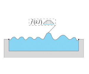
Figure 1 presents an illustration of the investigated configuration. Consider a shallow chamber of depth ${\tilde{h}_0}$ and length ${\tilde{l}_c}$ filled with a Newtonian liquid of mass density $\tilde{\rho }$, dynamic viscosity $\tilde{\mu }$ and volume $\tilde{V}$. The liquid-air interface has a surface tension $\tilde{\gamma }$ and is subjected to a normal force distribution $\tilde{f}(\tilde{x},\tilde{t})$ that induces a spatio-temporal deformation of the interface, $\tilde{h}(\tilde{x},\tilde{t})$. Under the assumptions of shallow geometry $({\tilde{h}_0} \ll {\tilde{l}_c})$ and negligible fluid inertia, the Navier–Stokes equations reduce to the lubrication equations

(2.1a–c)\begin{equation}{\tilde{u}_{\tilde{x}}} + {\tilde{w}_{\tilde{z}}} = 0,\quad {\tilde{p}_{\tilde{x}}} = \tilde{\mu }{u_{\tilde{z}\tilde{z}}},\quad {\tilde{p}_{\tilde{z}}} =- \tilde{\rho }\tilde{g}, \end{equation}

where $(\tilde{u},\tilde{w})$ are the velocity components in the $\tilde{x}$ and $\tilde{z}$ directions respectively, and $\tilde{p}$ is the fluidic pressure. We marked the derivative with respect to x of a multivariable function, $g(x,z)$, as ${g_x}$. Requiring no slip at the bottom surface, a stress balance at the free surface and utilizing the kinematic boundary condition, the equations can be further simplified to the Reynolds equation, (Oron et al. Reference Oron, Davis and Bankoff1997; Leal Reference Leal2007)

(2.2)\begin{equation}{\tilde{h}_{\tilde{t}}} = \frac{1}{{3\tilde{\mu }}}{({\tilde{h}^3}{\tilde{p}_{\tilde{x}}})_x}.\end{equation}

Under the longwave approximation (linear curvature), the fluidic pressure, $\tilde{p}$, is given by

(2.3)\begin{equation}\tilde{p} = \tilde{\rho }\tilde{g}(\tilde{h} - \tilde{z}) - \tilde{\gamma }{\tilde{h}_{\tilde{x}\tilde{x}}} - \tilde{f} + \tilde{C},\end{equation}

where the first term on the right-hand side is the hydrostatic pressure, the second one is the capillary pressure associated with the curvature of the interface, the third one is the normal stress distribution on the interface and $\tilde{C}$ is a constant. We denote the film deformation as $\tilde{d}(\tilde{x},\tilde{t}) = \tilde{h}(\tilde{x},\tilde{t}) - {\tilde{h}_0}$, and define the non-dimensional quantities $t = \tilde{t}/\tilde{\tau }$, $x = \tilde{x}/({\tilde{l}_c}/2)$, $d = \tilde{d}/{\tilde{h}_0}$, $f = \tilde{f}/\tilde{F}$. By further assuming small deformations, $d \ll 1$, we obtain the non-dimensional linearized evolution equation for the deformation

(2.4)\begin{equation}{d_t} + {d_{xxxx}} - Bo \times {d_{xx}} =- \varPi {f_{xx}},\end{equation}

where $Bo = \tilde{\rho }\tilde{g}\tilde{l}_c^2/4\tilde{\gamma }$ is the Bond number, $\varPi = \tilde{F}\tilde{l}_c^2/4\tilde{\gamma }{\tilde{h}_0}$ represents the non-dimensional interfacial force magnitude and the resulting time scale is $\tilde{\tau } = 3\tilde{\mu }\tilde{l}_c^4/16\tilde{h}_0^3\tilde{\gamma }$.

Figure 1.

(a) Two-dimensional illustration of the investigated model comprising a shallow chamber of length ${\tilde{l}_c}$ and height ${\tilde{h}_0}$ filled with a liquid of mass density $\tilde{\rho }$, dynamic viscosity $\tilde{\mu }$ and open to the air above. The liquid-air interface with surface tension $\tilde{\gamma }$ is subjected to a normal force distribution $\tilde{f}(\tilde{x},\tilde{t})$, resulting in a deformed liquid height $\tilde{h}(\tilde{x},\tilde{t})$. At the edges of the chamber the liquid is pinned and cannot penetrate the solid, resulting in global mass conservation. (b) The normal force distribution along the chamber at the liquid-air interface. (c) An illustration of a microfabricated chamber used in the experiments. The bottom of the chamber is patterned with an array of electrodes imposing a DEP force on the liquid-air interface. (d) Example of an experimentally observed deformation of the liquid film when subjected to a DEP force distribution.

At the boundaries we require the liquid to be pinned,

(2.5)\begin{equation}d(x ={\pm} 1,t) = 0,\end{equation}

as well as no penetration through the boundaries, i.e. $u(x ={\pm} 1,t) = 0$. Integrating the x-momentum equation (2.1b) with respect to $\tilde{z}$, yields $\tilde{u} = {\tilde{p}_{\tilde{x}}}(1/2\tilde{\mu })({\tilde{z}^2}/{\tilde{h}^2} - 2(\tilde{z}/\tilde{h}))$, which translates the no-penetration boundary conditions to ${\tilde{p}_{\tilde{x}}} = 0$ at the chamber edges. Applying this requirement to (2.3), yields the following boundary condition on the deformation:

(2.6)\begin{equation}{d_{xxx}}(x ={\pm} 1,t) - Bo \times {d_x}(x ={\pm} 1,t) =- \varPi {f_x}(x ={\pm} 1,t).\end{equation}

These boundary conditions are accompanied by an arbitrary initial condition, $d(x,t = 0) = {d_0}(x)$.

A straightforward approach for solving the system (2.4) with boundary conditions (2.5) and (2.6) is by separation of variables. However, as we detail here, this set of boundary conditions is responsible for transforming the system into a non-self-adjoint one, requiring special treatment in the separation of variables procedure. Equations (2.7)–(2.13) follow the standard procedure for separation of variables, yet we present it explicitly for completeness and consistency with the derivation in (2.14)–(2.19), where we construct the solution based on the adjoint operator.

We first homogenize the boundary conditions by expressing the deformation as $d(x,t) = \hat{d}(x,t) + P(x,t)$, $P(x,t)$ is the homogenizing function that should be selected as a polynomial of sufficient degree in x such that the source terms will vanish from all boundary conditions, yielding the system

(2.7) \begin{equation}\left. {\begin{array}{*{20}{c@{}}} {{{\hat{d}}_t} + {{\hat{d}}_{xxxx}} - Bo\times {{\hat{d}}_{xx}} =- {P_t} - \varPi {f_{xx}} - {P_{xxxx}} + Bo\times {P_{xx}}}\\ {\hat{d}(x ={\pm} 1,t) = 0}\\ {{{\hat{d}}_{xxx}}(x ={\pm} 1,t) - Bo \times {{\hat{d}}_x}(x ={\pm} 1,t) = 0}\\ {\hat{d}(x,t = 0) = {d_0}(x) - P(x,0)} \end{array}} \right\}.\end{equation}

A compact and convenient homogenizing function can be constructed from a third-order polynomial,

(2.8)\begin{equation}P(x,t) = \Pi \frac{{{f_x}(1,t) - {f_x}( - 1,t)}}{{4Bo}}({x^2} - 1) + \varPi \frac{{{f_x}(1,t) + {f_x}( - 1,t)}}{{4(Bo - 3)}}({x^3} - x),\end{equation}

which is valid for any Bond number except $Bo = 0,3$. To cover these two specific cases, a fourth-order polynomial can be constructed.

Next, by separation of variables, we suggest a solution in the form of $\hat{d}(x,t) = X(x)T(t)$ and substitute it into the homogeneous form of (2.7), which yields

(2.9)\begin{equation}{-}\frac{{T^{\prime}}}{T} = \frac{{{X^{(4 )}}}}{X} - Bo\frac{{X^{\prime\prime}}}{X} = {\lambda ^4}.\end{equation}

The eigenvalue problem, (2.9), followed by the set of boundary conditions

(2.10a,b)\begin{equation}X({\pm} 1) = 0,\quad X^{\prime\prime\prime}({\pm} 1) - BoX^{\prime}({\pm} 1) = 0,\end{equation}

where each prime denotes a derivation with respect to the single variable of the function. The solution of the system (2.9) and (2.10) is given by

(2.11) \begin{equation}{X_n} = \left\{ {\begin{array}{*{20}{@{}ll}} {\dfrac{{\sqrt {Bo} (\cosh (\sqrt {Bo} x) - \cosh (\sqrt {Bo} ))}}{{2(\sinh (\sqrt {Bo} ) - \sqrt {Bo} \cosh (\sqrt {Bo} ))}}}&{\textrm{for}\;n = 0}\\ {\sin ({\alpha_n}x) - \dfrac{{\sin ({\alpha_n})}}{{\sinh ({\beta_n})}}\sinh ({\beta_n}x)}&{\textrm{for}\;\textrm{odd}\;n\;\textrm{numbers}}\\ {\cos ({\alpha_n}x) - \dfrac{{\cos ({\alpha_n})}}{{\cosh ({\beta_n})}}\cosh ({\beta_n}x)}&{\textrm{for}\;\textrm{even}\;n\;\textrm{numbers}} \end{array}} \right.,\end{equation}

where

(2.12a,b)\begin{equation}{\alpha _n} = \sqrt {\frac{{ - Bo + \sqrt {B{o^2} + 4\lambda _n^4} }}{2}} \quad \textrm{and}\quad {\beta _n} = \sqrt {\frac{{Bo + \sqrt {B{o^2} + 4\lambda _n^4} }}{2}} .\end{equation}

The eigenvalues are calculated from two transcendental equations, one for each set of eigenfunctions respectively

(2.13)\begin{equation}\left. {\begin{array}{*{20}{c@{}}} {\alpha \tan (\alpha ) =- \beta \tanh (\beta )}\\ {\beta \tan (\alpha ) = \alpha \tanh (\beta )} \end{array}} \right\}.\end{equation}

We note that all eigenfunctions have a zero spatial integral, except for the zero eigenfunction that corresponds to a steady state solution for a non-actuated system, and its integral sets the volume in the chamber.

The eigenfunctions (2.11) are non-orthogonal to one another, which is an indication of the non-self-adjointness of the system. Nonetheless, we can proceed by using the biorthogonality relation of the system with its adjoint system, $\langle L[X],Y\rangle = \langle X,{L^ + }[Y]\rangle$, where $\langle U,V\rangle = \int_{ - 1}^1 {UV\,\textrm{d}\kern0.06em x} $ is the basic inner product, L is the original differential operator, ${L^ + }$ is the Lagrange adjoint differential operator and X and Y are their respective solutions. We define the spatial differential operator from (2.9) as $L[X] = {X^{(4)}} - BoX^{\prime\prime}$. Since this spatial differential operator has constant real coefficients and only even derivatives, we are guaranteed that the Lagrange adjoint operator, ${L^ + }$, is identical to L (Coddington & Levinson Reference Coddington and Levinson1955). Explicitly expanding the biorthogonality relation while integrating by parts and using the boundary conditions (2.10), yields

(2.14)\begin{equation}[X^{\prime\prime}Y^{\prime} + X^{\prime}Y^{\prime\prime}]_{ - 1}^1 = 0,\end{equation}

which can hold only if $Y^{\prime}({\pm} 1) = Y^{\prime\prime}({\pm} 1) = 0$, thus defining the complementary boundary conditions for Y. These conditions are clearly different from those for X, (2.10), and thus the problem is not self-adjoint.

The solution for the adjoint system is given by

(2.15)\begin{equation}{Y_n} = \left\{ {\begin{array}{*{20}{@{}ll}} 1&{\textrm{for}\;n = 0}\\ {\sin ({\alpha_n}x) - \dfrac{{{\alpha_n}\cos ({\alpha_n})}}{{{\beta_n}\cosh ({\beta_n})}}\sinh ({\beta_n}x)}&{\textrm{for}\;\textrm{odd}\;n\;\textrm{numbers}}\\ {\cos ({\alpha_n}x) + \dfrac{{{\alpha_n}\sin ({\alpha_n})}}{{{\beta_n}\sinh ({\beta_n})}}\cosh ({\beta_n}x)}&{\textrm{for}\;\textrm{even}\;n\;\textrm{numbers}} \end{array}} \right..\end{equation}

The transcendental equations for the two sets of eigenvalues (for odd and even $n$) are identical to those of the original system, and thus the eigenvalues are the same. The solution to the deformation can now be constructed by substituting the separation of variables expression, i.e. $\hat{d}(x,t) = \sum\nolimits_{n = 0}^\infty {{X_n}(x){T_n}(t)}$, to the non-homogenous equation, (2.7), yielding

(2.16) \begin{align}&\sum\limits_{n = 0}^\infty {{X_n}(x){{T^{\prime}}_n}(t)} + \sum\limits_{n = 0}^\infty {X_n^{(4)}(x){T_n}(t)} - Bo\sum\limits_{n = 0}^\infty {{{X^{\prime\prime}}_n}(x){T_n}(t)}\notag\\ &\quad = \sum\limits_{n = 0}^\infty {{X_n}(x){a_n}(t)} + \sum\limits_{n = 0}^\infty {{X_n}(x){{b^{\prime}}_n}(t)} ,\end{align}

where

(2.17a–c) \begin{align} {-}\varPi {f_{xx}} + Bo \times {P_{xx}} - {P_{xxxx}} &= \sum\limits_{n = 0}^\infty {{a_n}(t){X_n}(x)} ,\quad P(x,t) = \sum\limits_{n = 0}^\infty {{b_n}(t){X_n}(x)} ,\notag\\ {d_0} - P(x,0) &= \sum\limits_{n = 0}^\infty {{I_n}{X_n}(x)} .\end{align}

Multiplying equation (2.16) by ${Y_m}$ and integrating over the domain with respect to x, as well as using the initial condition in (2.7), yields

(2.18)\begin{equation}{T_n} = \int_{s = 0}^t {{\textrm{e}^{\lambda _n^4(s - t)}}[{a_n}(s) - {{b^{\prime}}_n}(s)]\,\textrm{d}s} + {\textrm{e}^{ - \lambda _n^4t}}{I_n}.\end{equation}

Thus, the solution for the deformation is given by $d(x,t) = \sum\nolimits_{n = 0}^\infty {{T_n}(t){X_n}(x)} + P(x,t)$.

For a general function $g(x)$ the series expansion by the system eigenfunctions is given by

(2.19a,b)\begin{equation}g(x) = \sum\limits_{n = 0}^\infty {{c_n}{X_n}(x)} ;\quad {c_n} = \frac{{\int_{ - 1}^1 {g(x){Y_n}\,\textrm{d}\kern0.06em x} }}{{\int_{ - 1}^1 {{X_n}{Y_n}\,\textrm{d}\kern0.06em x} }}.\end{equation}

We note that, since our system has real and constant coefficients as well as homogenous boundary conditions, and since its eigenvalues are real with no duplicity, we are guaranteed that the eigenfunctions of both the original and the adjoint systems form a complete set (Coddington & Levinson Reference Coddington and Levinson1955).

3. Dynamics of the non-self-adjoint closed-chamber system and comparison with self-adjoint periodic and open-chamber systems

In this section we present the behaviour of a thin liquid film within a closed chamber and compare it with classical solutions for self-adjoint configurations such as periodic and open-chamber problems (solutions for the self-adjoint problems in Appendix A). Table 1 lists the boundary conditions for each of these cases. In the closed-chamber problem (‘Closed’) the liquid is pinned at both edges and the side walls of the chamber are impermeable. In the open-chamber problem (‘Open’) the liquid is also pinned, but is free to flow in and out of the chamber (i.e. the total volume in the chamber can vary in time). In the periodic case (‘Periodic’), there is no physical chamber, but the boundary conditions define a domain where the film deformation and its derivatives at one end are equal to their values at the other end. For simplicity, we consider here the case of Bo = 0, but solutions for other Bond values are readily available and do not introduce a fundamental change in behaviour.

Table 1.

Summary of the three systems considered in this section.

Figure 2 presents the solutions of the deformation for all three systems, at different times, for a harmonic $(\,f = 0.5[1 - \cos (10{\rm \pi} x)])$, and for a Gaussian $(\,f = exp [ - 0.5{(x + 0.85)^2}/{0.05^2}])$ force distribution with an initially flat interface, ${d_0}(x) = 0$. At early times, for both actuations, the deformation of the liquid-air interface is roughly the same for all systems. However, with time, deviations begin to emerge from the boundaries inward.

Figure 2.

The effect of different sets of boundary conditions (BCs) on the film dynamics for harmonic (left column, l) and localized (right column, r) force distributions. (a) The external force distributions applied on the liquid-air interface along the chamber. (b–e) Comparison of the analytical solutions for the case of pinned film and impermeable boundaries (‘Closed chamber’, black dashed line), pinned film and permeable boundaries (‘Open chamber’, red dashed line) and ‘Periodic’ (light purple dashed line), at different times. All panels in the left column present half of the chamber, with a symmetry line at x = 0. At early times, the deformation exhibited by all systems is nearly identical. With time, deviations start evolving from the boundaries inward. At the harmonic forcing case, since the force is strictly positive, the Open system results in a continuous influx of liquid which ultimately leads to inflation of the interface to a ‘balloon’-like structure. In contrast, the Closed and the Periodic systems, owing to their fixed mass, maintain short-wave deformations which follow the force distribution even at steady state, as shown in (e.l). The film deformation of the Open system at late times is much larger than the deformation of the other two systems. Thus, (d.l) and (e.l) present two different y axes, left for Closed and Periodic systems, and right for the Open system. In the Gaussian forcing case the Open and the Closed systems show similar behaviour due to the pinning condition (although the latter is not a fixed-volume system) in contrast to the Periodic system. The solution presented for all systems is for the case of an initially flat interface, ${d_0}(x) = 0$ and $Bo = 0$.

We note that the harmonic force is strictly positive. In the Open case, which allows for liquid influx, we see that this positive force results in ‘ballooning’ of the film and dominance of the lowest wavenumber. In contrast, in the Closed and Periodic systems, mass conservation does not allow for such inflation and the deformation follows the wavenumber of the force. Another key difference between the systems is that the amplitude of the deformation in the Open system is significantly larger (note the two different y-axes in figures 2d.l and 2e.l). For the localized force, the deformation in the Closed system resembles that of the Open system (although the former is mass conserving, and the latter is not). The most significant difference is seen here in comparison with the Periodic system in which the film height at the boundary is not fixed, resulting in much greater deformation (albeit mass conserving, i.e. both positive and negative deformations are accentuated). Thus, we can see from the results that neither the Open nor the Periodic formulations can correctly model the dynamics of a Closed system.

Figure 2 shows that the Open, Closed and Periodic systems reach a steady state at different times. In figure 2, the localized actuation (right column) triggers a range of system eigenfunctions, and the time to steady state scales as ${\lambda ^{ - 4}}$, where $\lambda $ is the first (slowest) eigenvalue. The eigenvalues of the system are of course dependent on its boundary conditions. For example, at $Bo = 0$, the time scales for steady state in the Open, Closed and Periodic systems are respectively $\tilde{\tau }{(2/{\rm \pi})^4}$, $\tilde{\tau }{(1/2.37)^4}$ and $\tilde{\tau }{(1/{\rm \pi})^4}$. i.e. the Closed system is 5-fold faster than the Open system, but 3-fold slower than the Periodic system. Thus, solving for the accurate eigenvalues, meaning using the correct boundary conditions of the system is crucial in order to properly predict the system dynamics.

4. Effect of Bond number on system dynamics: response time and deformation magnitude

In this section we investigate the relation between the Bond number and both the response time of the system and the magnitude of the deformation at steady state. The liquid pressure is constant at steady state, thus substituting the non-dimensional parameters defined in (2.4) into (2.3) yields

(4.1)\begin{equation}{d_{xx}} - Bo \times d + \varPi \times f = C,\end{equation}

where C is a constant that depends on the liquid volume. For the case of large Bond numbers, $Bo \gg 1$, the deformation can be written as $d \approx \varPi f/Bo + \textrm{const}\textrm{.}$ We note that this equation holds only sufficiently far from the chamber edges; close to the edges, the requirement for mass conservation together with pinning conditions may result in significant curvatures, i.e. non-negligible ${d_{xx}}$.

While $\tilde{\tau }$ was conveniently defined in (2.4) as being independent of the Bond number, the response time of the system is in fact strongly influenced by it, as indicated by the relation between the eigenvalues and the Bond number in (2.11). This influence is further enhanced through the quartic dependence of the time scale on the system eigenvalues, ${\lambda _n}$. The eigenvalues can be obtained by solving a pair of transcendental equations (2.13), for the odd and the even eigenvalues

(4.2a)\begin{gather}\sqrt {\frac{{ - Bo + \sqrt {B{o^2} + 4\lambda _n^4} }}{{Bo + \sqrt {B{o^2} + 4\lambda _n^4} }}} \tan \left(\! {\sqrt {\frac{{ - Bo + \sqrt {B{o^2} + 4\lambda_n^4} }}{2}} } \right) =- \tanh \left(\! {\sqrt {\frac{{Bo + \sqrt {B{o^2} + 4\lambda_n^4} }}{2}} } \right)\!\!,\end{gather}

(4.2b)\begin{gather}\sqrt {\frac{{ - Bo + \sqrt {B{o^2} + 4\lambda _n^4} }}{{Bo + \sqrt {B{o^2} + 4\lambda _n^4} }}} \tanh \left( {\sqrt {\frac{{Bo + \sqrt {B{o^2} + 4\lambda_n^4} }}{2}} } \right) = \tan \left( {\sqrt {\frac{{ - Bo + \sqrt {B{o^2} + 4\lambda_n^4} }}{2}} } \right).\end{gather}

The solid lines in figure 3 present the dependence of the resulting non-dimensional response time, ${\lambda ^{ - 4}}$, on Bo. For large Bond numbers, the asymptotic solutions for the eigenvalues are simply ${\lambda _1} = \sqrt {{\rm \pi}/2} B{o^{1/4}}$ and ${\lambda _2} = \sqrt {\rm \pi}B{o^{1/4}}$, and are indicated by the black and the grey dashed lines, respectively. For clarity, the square, circle, and x markers indicate the time scale at specific Bond numbers listed in the figure's legend. Clearly, the effect of Bo can be quite significant; the same system at Bo = 0 would have a response time 84-fold slower than the same system at $Bo = 1000$.

Figure 3.

The eigenvalues of the system as a function of the Bond number. The response time of the system is proportional to $\lambda^{-4}$, which for large Bo is inversely proportional to Bo. Thus, as Bo increases, e.g. by increasing the density of the liquid or increasing the size of the container, the response time of the system can shorten significantly.

5. Experimental validation

5.1. Experimental set-up

To experimentally study the dynamics of thin-film deformation, we fabricated a shallow fluidic chamber with embedded electrodes which can impose a DEP force on the interface of a thin liquid film resting in the chamber. The chamber is 4 mm long, 8 mm wide and 50 μm deep (as shown in figure 4a). We filled it with 1.6 μl of silicone oil which has a mass density of $\tilde{\rho } = 970\;\textrm{kg}\;{\textrm{m}^{ - \textrm{3}}}$, surface tension of $\tilde{\gamma } = 21 \times {10^{ - 3}}\;\textrm{N}\;{\textrm{m}^{ - 1}}$ and electric permittivity of $\tilde{\varepsilon } = 2.7{\tilde{\varepsilon }_0}$, where ${\tilde{\varepsilon }_0}$ is the permittivity of free space. The bottom of the chamber is patterned with an array of 200 μm wide parallel electrodes, gapped by 200 μm edge to edge. By introducing a sinusoidal electric potential difference to the electrodes (500 Vpp, 10 kHz), the resulting localized electric field imposes DEP forces on the oil-air interface and deforms it. Figure 4(b) presents the digital holographic microscope (Cuche, Marquet & Depeursinge Reference Cuche, Marquet and Depeursinge1999) we used to observe the time-dependent deformation of the interface. For each experiment, we initially acquire the baseline surface topography prior to activation of the electric field, and then subtract it from all subsequent measurements.

Figure 4.

Illustration of the fluidic chamber the experimental set-up. (a) The resulted fluidic chamber configuration and it's fabrication process. At first, the electrodes are created by a lift-off process using a 2 nm thick Pt layer sandwiched between two 2 nm thick Ti layers on a borosilicate wafer which forms an array of interdigitated electrode configuration with 200 μn wide electrodes, gapped by 200 μm edge to edge. Second, the chamber's walls are created by patterning a 50 μm thick layer of SU-8 photoresist on top of the wafer. Finally, we diced the wafer to separate individual devices. (b) Schematic illustration of the experimental set-up. The device is mounted on a home-made connector composed of 3D printed housing and a printed circuit board (PCB) containing electric pins interfacing the device with a voltage amplifier (2210-CE, TREK), which amplifies the voltage output of a wave generator (TG5012A, AIM-TTI Instruments). The device is placed under a digital holographic microscope (DHM R1000, Lyncee tec) allowing observation of the oil-air interface by recording a hologram image on a digital sensor and using a numerical algorithm for real-time reconstruction.

5.2. Experimental results

Figure 5 compares the experimental measurements with an analytical solution based on (2.4). The analytical solution is obtain using the force distribution presented in figure 5(a), corresponding to the DEP force on a liquid-air interface from periodic electrodes (Gabay et al. Reference Gabay, Paratore, Boyko, Ramos, Gat and Bercovici2021). Figure 5(b–f) presents the evolution of the film in time, showing the gradual appearance of the different spatial modes. At very early times (0.2 ms) the highest spatial frequency is dominant, and the ‘tooth’-shaped peaks of the force distribution are also clearly observable in the analytical solution for the deformation. At 2 ms, the model and the experimental measurements agree well and show that the tenth even mode of the system has grown significantly (note the change in scale from nm to μm) and dominates the solution. The amplitude of the periodic deformation steadily increases, until at 37 ms a new qualitative change appears, initially in the form of a larger amplitude wave that penetrates from the boundaries. This is predicted well by the analytical model in good agreement with the experiments. By 3.55 s, the entire central region of the liquid has risen at the expense of the edges. The results continue to show good agreement, although some asymmetry begins to appear in the experimental measurements, resulting in slightly larger quantitative deviations. This is likely due to an additional low spatial frequency of the force distribution in the experiment that is not captured by the analytical force model, and which therefore appears only at long times. At 100 s the system has achieved its steady state. The deformation at the centre of the chamber is strictly positive. The overall shape and multitude of spatial frequencies is captured well by the theory, although quantitative differences, particularly on the right side of the chamber, are now evident.

Figure 5.

Validation of the analytical model against experimental measurements. (a) The DEP force distribution at the oil-air interface resulting from an array of parallel electrodes, as obtained from an electrostatic calculation in accordance with Gabay et al. (Reference Gabay, Paratore, Boyko, Ramos, Gat and Bercovici2021). (b–f) The evolution of the film deformation from early times to steady state, showing the dominance of high wavenumbers at short times, and the gradual appearance of small wavenumbers with time. The analytical model successfully captures both the local and the global behaviour of the film across multiple time scales. The chamber length is 4 mm, and is thus slightly truncated on the right by the 3.8 mm field of view of the holographic microscope. In this experiment we use silicone oil with kinematic viscosity of $200\ \textrm{cSt}$.The rest of the parameters (liquid properties and electric voltage actuation) are listed in the § 5.1.

We note that figure 5(b) (representing the deformation at 0.2 ms, or $t = 5 \times {10^{ - 8}}$ in non-dimensional time) does not include experimental results, as this time scale was too short for our imaging system to capture. To overcome this limitation, we conducted an additional experiment using silicone oil with a kinematic viscosity five times higher (1000 cSt) than the one presented in figure 5 (200 cSt). Additionally, we reduced the liquid volume, resulting in a thinner film. Both modifications increased the hydrodynamic resistance of the system and consequently led to an order of magnitude slower dynamics such that t = 2.44 × 10⁻⁸ corresponds to 2 ms. Despite the reduced liquid volume, the liquid remained pinned at the edges of the chamber, resulting in initial conditions where the film had a bowl shape with a height of 50 μm at the edges and approximately 20 μm at the centre of the chamber. We compared the experimental measurements with an analytical solution assuming a film with a uniform height of 30 μm, which corresponds to the average film thickness in the chambers.

In figure 6(a), we present the force distribution at the interface, characterized by ‘tooth'-shaped peaks with the smallest wavelength in the system, arising from the transition region between adjacent electrodes. As discussed in § 3, large spatial wavenumbers are associated with a rapid temporal response. To isolate these features, we need to focus on short times. Figure 6(b–f) depicts the deformation of the film at different time points. At 2 ms, only the highest spatial frequency is visible, in good agreement with the analytical prediction. By 22 ms, a longer wavelength becomes distinctly visible and, as time progresses, it becomes the dominant feature of the deformation.

Figure 6.

Validation of the analytical model with experimental measurements at very small non-dimensional times, $t < {10^{ - 6}}$. (a) The DEP force distribution at the oil--air interface of a 30 μm film, as obtained from electrostatic calculations (Gabay et al. Reference Gabay, Paratore, Boyko, Ramos, Gat and Bercovici2021). (b–f) Comparison between the analytical solution (black dashed line) and the experimental measurements (black solid line) of the film deformations at different times. At short times the ‘tooth’-shaped peaks, corresponding to the highest spatial frequency, dominate the deformation. At later times, additional lower frequencies appear and overtake the higher frequencies in amplitude. In this experiment we use silicone oil with kinematic viscosity of $1000\ \textrm{cSt}$. The rest of the parameters (liquid properties and electric voltage actuation) are listed in § 5.1.

6. Concluding remarks

Thin liquid films are found in endless applications such as spin coating, self-healing and printing technologies, where infinite boundary conditions are appropriate for describing the film dynamics. However, there is an entire class of problems that inherently rely on no-penetration boundary conditions. For example, in liquid-based actuators, such as the ones used for adaptive optics (Banerjee et al. Reference Banerjee, Rajaeipour, Ataman and Zappe2018), enclosed chambers with a fixed amount of liquid are naturally the most common implementation. Banerjee et al. have already shown the use of a membrane suspended over a thin liquid film as a mechanism for achieving freeform optical corrections with up to fourth degree Zernike polynomials. However, the performance of such devices could not be predicted a priori, as no theory was available. The model we developed here provides insight into such systems and reveals the underlying eigenfunctions and their individual and collective dynamics. For diffractive optical components, the variations in surface topography are of the order of a wavelength, and thus the solution in the small deformation regime is suitable. Clearly, for larger deformations the nonlinear equation must be considered and would yield different quantitative results, but it is reasonable to expect that the boundary conditions would have a dominant effect as well. While our derivations focused on a free interface, they directly apply to the case of a membrane under dominant tension, and could also be readily extended to account for elastic bending. However, in order to quantitatively predict the response of actuation devices, the theory must be extended to two-dimensional domains.

The Closed system's boundary conditions affect both the shape of the liquid film for a long time scale and the characteristic time scales required to achieve steady state. While obtaining the shape of the interface for the closed system requires solving the adjoint problem, the time scales can be readily obtained from solving the transcendental equation of the original operator. The time scale analysis shows that the Closed system is 5-fold faster than the Open system and 3-fold slower than the Periodic one. We further showed that neither the open nor the periodic solutions can reasonably predict the deformation of the thin liquid film for general actuations. Another set of boundary conditions that is often used in the study of thin-film dynamics is that of an infinite film. We did not explicitly consider this case as it's a subset of an Open system where the domain size is stretched to infinity. It thus suffers from the same issues as the open case, namely dominance of low wavenumber eigenfunctions (‘ballooning’) at long times.

In figure 3 we presented the effect of Bond number on the eigenvalues of the of system, representing the non-dimensional time scale of the corresponding eigenfunctions. The figure shows that increasing the Bond number increases the eigenvalues and shortens the response time. However, to understand the effect of the physical parameters on the response time of the system we must consider the dimensional time scale, $\tilde{t} \propto \tilde{\tau }{\lambda ^{ - 4}}$. The effect of density changes, $\tilde{\rho }$, is straightforward as it appears only in the dependence of $\lambda $ on Bo. However, an increase in surface tension $\tilde{\gamma }$ results in a decrease in time scale through $\tilde{\tau }$ and an increase in time scale through Bo. At low Bo, the $\tilde{\tau }$ dependence dominates and increasing the surface tension will decrease the time scale. At large Bond numbers, the increase in time scale through $\tilde{\tau }$ will balance its decrease through the Bond number and the system becomes insensitive to the value of the surface tension.

In our derivation we focused on the case of normal forces applied directly to the liquid-air interface and implemented it using DEP. However, for other actuation mechanisms such as those that dictate a slip velocity electro-osmotic flow (EOF) or an interface velocity (thermocapillary flow), the differential operator and the impermeability boundary conditions would be identical. The only thing that would differ is the right-hand side of (2.4) (Rubin et al. Reference Rubin, Tulchinsky, Gat and Bercovici2017), but that would not change the solution procedure. When dictating a spatial force/velocity distribution in combination with the evolution equation, (2.2), care should be taken not to violate the underlying assumptions, at least not at the leading order of the solution; e.g. if dictating a slip velocity, then no penetration at the domain boundaries would be fully satisfied under the lubrication approximation only if its magnitude and its spatial derivative vanish at the boundary.

Finally, we note that the non-self-adjointness is a manifestation of the mass conservation constraint on the system, and is likely to appear in other fluidic problems that are subjected to similar constraints, as well as in their numerical solutions.