





1 Introduction
Let F be a local field with residue field
$\mathbb {F}_q$
 of order q, a power of p. Let l be a prime distinct from p, and let
$E/\mathbb {Q}_l$
of order q, a power of p. Let l be a prime distinct from p, and let
$E/\mathbb {Q}_l$
 be a finite extension with ring of integers
$\mathcal {O}$
be a finite extension with ring of integers
$\mathcal {O}$
 and residue field
$\mathbb {F}$
and residue field
$\mathbb {F}$
 . The (framed) moduli space of Langlands parameters for
$GL_n$
. The (framed) moduli space of Langlands parameters for
$GL_n$
 over
$\mathcal {O}$
over
$\mathcal {O}$
 parametrizes continuous homomorphisms

for
$\mathcal {O}$
 -algebras R, where
$W_F^0$
-algebras R, where
$W_F^0$
 is a certain choice of discretization of the Weil group of F. It has been intensely studied in recent years due to its role in modularity lifting theorems (e.g., [Reference Kisin15] and [Reference Clozel, Harris and Taylor4]) and, more recently, in geometrization of the local Langlands conjecture as in [Reference Zhu24], [Reference Fargues and Scholze7], [Reference Hellmann11], and [Reference Ben-Zvi, Chen, Helm and Nadler2]; the analogous object for arbitrary reductive groups was constructed in [Reference Dat, Helm, Kurinczuk and Moss5], [Reference Fargues and Scholze7], and [Reference Zhu24].
There is a very explicit presentation for the clopen subscheme of tame parameters: it is isomorphic to the
$\mathcal {O}$
 -scheme
$\mathcal {M} = \mathcal {M}_{n,q}$
-scheme
$\mathcal {M} = \mathcal {M}_{n,q}$
 whose R-points, for
$\mathcal {O}$
whose R-points, for
$\mathcal {O}$
 -algebras R, are given by

This has a number of pleasant geometric properties: it is an affine complete intersection over
$\mathcal {O}$
 , equidimensional of relative dimension
$n^2$
, equidimensional of relative dimension
$n^2$
 , it is flat over
$\mathcal {O}$
, it is flat over
$\mathcal {O}$
 , and it is reduced (see [Reference Dat, Helm, Kurinczuk and Moss5] section 2).
The geometric irreducible components of
$\mathcal {M}$
 are in bijection with q-power stable conjugacy classes in
$GL_n(\overline {E})$
are in bijection with q-power stable conjugacy classes in
$GL_n(\overline {E})$
 . In applications of the Taylor–Wiles–Kisin method, as well as in the analysis of the functors conjectured in [Reference Zhu24] and [Reference Fargues and Scholze7], it is natural to consider various unions of irreducible components of
$\mathcal {M}$
. In applications of the Taylor–Wiles–Kisin method, as well as in the analysis of the functors conjectured in [Reference Zhu24] and [Reference Fargues and Scholze7], it is natural to consider various unions of irreducible components of
$\mathcal {M}$
 obtained by restricting the conjugacy class of
$\Sigma $
obtained by restricting the conjugacy class of
$\Sigma $
 (the ‘type’). For
$n = 2$
(the ‘type’). For
$n = 2$
 , very explicit equations for these fixed-type deformation rings were constructed by the second author in [Reference Shotton19, Reference Hu and Paškūnas13]. As a result, they were shown to be Cohen–Macaulay.
In this article we consider the Steinberg component
$\mathcal {X}_{\operatorname {St}}$
 defined to be the Zariski closure of the open subset of
$\mathcal {M}(\overline {E})$
defined to be the Zariski closure of the open subset of
$\mathcal {M}(\overline {E})$
 on which
$\Sigma $
on which
$\Sigma $
 is a regular unipotent matrix:

Our main theorem is then:
Theorem 1.1. Let
$n = 2$
 or
$3$
or
$3$
 and suppose that
$l> n$
and suppose that
$l> n$
 and that

Then
$\mathcal {X}_{\operatorname {St}}$
 is Cohen-Macaulay and
$\mathcal {X}_{\operatorname {St}, \mathbb {F}}$
is Cohen-Macaulay and
$\mathcal {X}_{\operatorname {St}, \mathbb {F}}$
 is normal and reduced.
Under the same hypotheses, we also obtain a complete set of equations for
$\mathcal {X}_{\operatorname {St}}$
 as a closed subscheme of
$GL_n \times GL_n$
as a closed subscheme of
$GL_n \times GL_n$
 ;
a priori
, it is defined only as a Zariski closure. See Corollaries 5.4 and 5.8.
;
a priori
, it is defined only as a Zariski closure. See Corollaries 5.4 and 5.8.
When
$n = 2$
 this theorem (except the very last part) was essentially proved by the second author in [Reference Shotton19] by explicit methods, but we reprove it here more geometrically. The calculations of [Reference Shotton19] were applied by Manning in [Reference Manning17] to compute the Weil divisor class group of
$\mathcal {X}_{\operatorname {St}, \mathbb {F}}$
this theorem (except the very last part) was essentially proved by the second author in [Reference Shotton19] by explicit methods, but we reprove it here more geometrically. The calculations of [Reference Shotton19] were applied by Manning in [Reference Manning17] to compute the Weil divisor class group of
$\mathcal {X}_{\operatorname {St}, \mathbb {F}}$
 . This was combined with the Taylor–Wiles–Kisin patching method and a certain self-duality argument to identify the ‘patched module’ as an element of the class group and deduce multiplicity
$2^k$
. This was combined with the Taylor–Wiles–Kisin patching method and a certain self-duality argument to identify the ‘patched module’ as an element of the class group and deduce multiplicity
$2^k$
 results for the mod l cohomology of Shimura curves (and sets) associated to division algebras ramified at p.
For
$GL_3$
 we prove
Theorem 1.2. When
$n = 3$
 , the Weil divisor class group of
$\mathcal {X}_{\operatorname {St}, \mathbb {F}}$
, the Weil divisor class group of
$\mathcal {X}_{\operatorname {St}, \mathbb {F}}$
 is isomorphic to
$\mathbb {Z} \times \mathbb {Z}/3\mathbb {Z}$
is isomorphic to
$\mathbb {Z} \times \mathbb {Z}/3\mathbb {Z}$
 .
.
Our methods also give a new method to calculate the Weil divisor class group when
$n = 2$
 , which Manning did using toric geometry; for
$n = 3$
, which Manning did using toric geometry; for
$n = 3$
 the variety is no longer toric.
Unlike for
$n = 2$
 , the expected self-duality property does not specify a unique element of the class group (rather, there are three possibilities). When
$n = 3$
, the expected self-duality property does not specify a unique element of the class group (rather, there are three possibilities). When
$n = 3$
 , therefore, we do not make a precise conjecture for what the patched module should be, nor a multiplicity conjecture. That being said, forthcoming work of Helm–Manning is expected to provide another duality result for the patched module that would be sufficient to identify it uniquely. There are a number of other technical problems to be solved to carry out Manning’s argument in the case
$n = 3$
, therefore, we do not make a precise conjecture for what the patched module should be, nor a multiplicity conjecture. That being said, forthcoming work of Helm–Manning is expected to provide another duality result for the patched module that would be sufficient to identify it uniquely. There are a number of other technical problems to be solved to carry out Manning’s argument in the case
$n = 3$
 ; see Section 6.3 for further discussion.
The Steinberg component was previously considered by the first author [Reference Funck9], in which he showed that
$\mathcal {X}_{\operatorname {St}}$
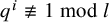
 is smooth when l is a banal prime, meaning that
$q^i \not \equiv 1 \bmod l$
is smooth when l is a banal prime, meaning that
$q^i \not \equiv 1 \bmod l$
 for
$1 \le i \le n$
for
$1 \le i \le n$
 . In fact he proved an analogous result for general G when q is ‘considerate’ towards l, a notion related to (but not identical with) the generalizations of ‘banal’ considered in [Reference Dat, Helm, Kurinczuk and Moss5]. This paper in some sense deals with the other extreme, when
$q \equiv 1 \bmod l$
. In fact he proved an analogous result for general G when q is ‘considerate’ towards l, a notion related to (but not identical with) the generalizations of ‘banal’ considered in [Reference Dat, Helm, Kurinczuk and Moss5]. This paper in some sense deals with the other extreme, when
$q \equiv 1 \bmod l$
 , sometimes called the quasi-banal case (if
$l> n$
, sometimes called the quasi-banal case (if
$l> n$
 ).
).
We use the method developed by Snowden [Reference Snowden21] to study ordinary deformation rings. The idea is to consider a projective resolution of
$\mathcal {X}_{\operatorname {St}}$
 by the variety obtained by adding a choice of Borel subgroup containing
$\Phi $
by the variety obtained by adding a choice of Borel subgroup containing
$\Phi $
 and
$\Sigma $
and
$\Sigma $
 . This variety fibres over the flag variety for
$GL_3$
. This variety fibres over the flag variety for
$GL_3$
 , and the desired properties of
$\mathcal {X}_{\operatorname {St}}$
, and the desired properties of
$\mathcal {X}_{\operatorname {St}}$
 can then be proved by computing (enough of) the cohomology of certain vector bundles on the flag variety. The methods for computing these cohomology groups are mostly due to Vilonen and Xue [Reference Vilonen and Xue23], and Ngo [Reference Ngo18], who were motivated by generalizing Snowden’s work in [Reference Snowden21] on ordinary deformation rings; however, we have to go beyond their calculations due to the subtleties of working in positive characteristic and also to obtain our results on explicit equations and multiplicities. The idea of applying this method in the
$l \ne p$
can then be proved by computing (enough of) the cohomology of certain vector bundles on the flag variety. The methods for computing these cohomology groups are mostly due to Vilonen and Xue [Reference Vilonen and Xue23], and Ngo [Reference Ngo18], who were motivated by generalizing Snowden’s work in [Reference Snowden21] on ordinary deformation rings; however, we have to go beyond their calculations due to the subtleties of working in positive characteristic and also to obtain our results on explicit equations and multiplicities. The idea of applying this method in the
$l \ne p$
 setting is also original to this paper.
Similar resolutions play a role in the ‘generalized Springer theory’ of [Reference Zhu24] and [Reference Ben-Zvi, Chen, Helm and Nadler2] and it would be interesting to compare our results with Conjecture 4.5.1 of [Reference Zhu24]; however, we will not do this here.
For higher values of n we still expect
$\mathcal {X}_{\operatorname {St}}$
 to be Cohen–Macaulay, but we are not able to prove it with our methods. Firstly, the cohomological calculations that we rely on become more difficult (for some examples, see [Reference Vilonen and Xue23]) and we do not have a general method for dealing with them. Secondly, we need good control of the variety of pairs of commuting upper triangular matrices; but for large enough n, this variety is not well-understood and lacks many desirable properties (e.g., it is not even equidimensional, see [Reference Basili1]). There is some hope of extending our calculation of the divisor class group in Section 6 to higher values of n, as one can work after removing a closed subset of codimension at least 2.
Here is an outline of the paper. In Section 2 we define the resolution we need and explain how Theorem 1.1 follows from properties that hold for its special fibre. In Section 3 we prove these properties modulo calculations of the cohomology of vector bundles on the flag variety; we carry out these calculations in Section 4. In Section 5 we obtain explicit equations for
$\mathcal {X}_{\operatorname {St}}$
 . In Section 6 we use our resolution to compute the Weil divisor class group of
$\mathcal {X}_{\operatorname {St}, \mathbb {F}}$
. In Section 6 we use our resolution to compute the Weil divisor class group of
$\mathcal {X}_{\operatorname {St}, \mathbb {F}}$
 and identify the canonical class inside it. We identify the divisorial sheaves satisfying the expected self-duality, and compute their multiplicities.
2 Resolution of Steinberg deformation rings
We let p, q, l,
$\mathcal {O}$
 , E and
$\mathbb {F}$
, E and
$\mathbb {F}$
 be as in the introduction, let
$n \ge 1$
be as in the introduction, let
$n \ge 1$
 be an integer, and consider the Steinberg component
$\mathcal {X}_{\operatorname {St}}$
be an integer, and consider the Steinberg component
$\mathcal {X}_{\operatorname {St}}$
 as defined in the introduction; equivalently,
$\mathcal {X}_{\operatorname {St}}$
as defined in the introduction; equivalently,
$\mathcal {X}_{\operatorname {St}}$
 is the Zariski closure of

inside
$GL_{n,\mathcal {O}} \times GL_{n,\mathcal {O}}$
 .
.
From now on, we assume:
Assumption 2.1. We have
$l> n$
 and
$q \equiv 1 \bmod l$
and
$q \equiv 1 \bmod l$
 .
.
On
$\mathcal {X}_{St}$
 , the eigenvalues of
$\Phi $
, the eigenvalues of
$\Phi $
 are in the ratio
$1:q:\ldots :q^{n-1}$
are in the ratio
$1:q:\ldots :q^{n-1}$
 . Since
$q \equiv 1 \mod l$
. Since
$q \equiv 1 \mod l$
 and
$l \nmid n$
and
$l \nmid n$
 , there is then an isomorphism
$\mathbb {G}_m \times \mathcal {X} \xrightarrow {\sim } \mathcal {X}_{\operatorname {St}}$
, there is then an isomorphism
$\mathbb {G}_m \times \mathcal {X} \xrightarrow {\sim } \mathcal {X}_{\operatorname {St}}$
 where
where

It will be technically more convenient to work with
$\mathcal {X}$
 . Here
$\operatorname {char}_{\Phi }(T)$
. Here
$\operatorname {char}_{\Phi }(T)$
 is the characteristic polynomial of
$\Phi $
is the characteristic polynomial of
$\Phi $
 .
.
As
$l> n$
 , the logarithm map
$\Sigma \mapsto \log (\Sigma -1)$
, the logarithm map
$\Sigma \mapsto \log (\Sigma -1)$
 is well defined for unipotent
$\Sigma $
is well defined for unipotent
$\Sigma $
 and hence on
$\mathcal {X}$
and hence on
$\mathcal {X}$
 we may write
$\Sigma = \exp (N)$
we may write
$\Sigma = \exp (N)$
 for a nilpotent matrix
$N \in \mathfrak {g}$
for a nilpotent matrix
$N \in \mathfrak {g}$
 , where
$\mathfrak {g}$
, where
$\mathfrak {g}$
 is the Lie algebra of
$GL_n$
is the Lie algebra of
$GL_n$
 ; the defining equation then becomes
$\Phi N \Phi ^{-1} = qN$
; the defining equation then becomes
$\Phi N \Phi ^{-1} = qN$
 . In what follows we will describe points on
$\mathcal {X}$
. In what follows we will describe points on
$\mathcal {X}$
 in the form
$(\Phi , N)$
in the form
$(\Phi , N)$
 .
.
We let
$X = \mathcal {X}_{\mathbb {F}}^{\operatorname {red}}$
 ; it will follow from our work below that

which is irreducible. This fact also follows from the results of [Reference Shotton20] Section 7.
2.1 Resolution of
$\mathcal {X}$


Let
$B \subset GL_n$
 be the standard Borel subgroup with Lie algebra
$\mathfrak {b}$
be the standard Borel subgroup with Lie algebra
$\mathfrak {b}$
 ; let N be its unipotent radical, with Lie algebra
$\mathfrak {n}$
; let N be its unipotent radical, with Lie algebra
$\mathfrak {n}$
 . Let
$\mathcal {F} \cong G/B$
. Let
$\mathcal {F} \cong G/B$
 be the flag variety; for an
$\mathcal {O}$
be the flag variety; for an
$\mathcal {O}$
 -algebra R, we can write a point
$F \in \mathcal {F}(R)$
-algebra R, we can write a point
$F \in \mathcal {F}(R)$
 as a flag
$0 \subset F_{n-1} \subset \ldots \subset F_0 = R^n$
as a flag
$0 \subset F_{n-1} \subset \ldots \subset F_0 = R^n$
 with the
$F_i$
with the
$F_i$
 projective R-modules such that
$\mathrm {gr}_i(F_{\bullet })$
projective R-modules such that
$\mathrm {gr}_i(F_{\bullet })$
 are all projective. We define
$\mathcal {Z}$
are all projective. We define
$\mathcal {Z}$
 to be the closed subscheme of
$G \times \mathfrak {g} \times \mathcal {F}$
to be the closed subscheme of
$G \times \mathfrak {g} \times \mathcal {F}$
 given (on R-points) as the set of triples
$(\Phi , N, F)$
given (on R-points) as the set of triples
$(\Phi , N, F)$
 such that

and

for
$i = 0, \ldots , n-1$
 . We define
$\mathcal {Y} \subset \mathcal {Z}$
. We define
$\mathcal {Y} \subset \mathcal {Z}$
 as the closed subscheme with

We thus have a closed embedding
$\mathcal {Y}\hookrightarrow \mathcal {Z}$
 fitting into the diagram below:

Lemma 2.2. The morphism
$f : \mathcal {Y} \to \mathcal {X}$
 given by forgetting F is a projective morphism. It is an isomorphism over the open subset of
$\mathcal {X}$
given by forgetting F is a projective morphism. It is an isomorphism over the open subset of
$\mathcal {X}$
 on which N is regular or l is invertible.
Proof. The scheme
$\mathcal {Y}$
 is a closed subscheme of
$\mathcal {X}\times \mathcal {F}$
is a closed subscheme of
$\mathcal {X}\times \mathcal {F}$
 and
$\mathcal {F}$
and
$\mathcal {F}$
 is projective, thus
$\mathcal {Y} \to \mathcal {X}$
is projective, thus
$\mathcal {Y} \to \mathcal {X}$
 is projective. Let U denote the open subset of
$\mathcal {X}$
is projective. Let U denote the open subset of
$\mathcal {X}$
 on which N is regular or l is invertible. We write down an inverse to f on U by writing down the required flag for each R-point
$(\Phi , N)$
on which N is regular or l is invertible. We write down an inverse to f on U by writing down the required flag for each R-point
$(\Phi , N)$
 of U:
of U:
-
• When N is regular (that is, its value at each point of $\operatorname {Spec} R$
is regular), take
$F_i = \ker (N^{n-i})$
; -
• When l is invertible, take $F_i=\bigoplus _{j=i}^{n-1} \ker (\Phi -q^i)$
.



The relation
$\Phi N \Phi ^{-1} = qN$
 implies that these agree on the locus where N is regular and l is invertible, and one can check that this defines a two-sided inverse
$U \to f^{-1}(U) \subset \mathcal {Y}$
implies that these agree on the locus where N is regular and l is invertible, and one can check that this defines a two-sided inverse
$U \to f^{-1}(U) \subset \mathcal {Y}$
 of
$f|_{f^{-1}(U)}$
of
$f|_{f^{-1}(U)}$
 .
.
Lemma 2.3.
-
1. The scheme $\mathcal {Z}$
is an affine bundle over
$\mathcal {F}$
; in particular, it is
$\mathcal {O}$
-flat and
$\mathcal {Z}_{\mathbb {F}}$
is reduced and irreducible. -
2. If $n \le 3$
,
$\mathcal {Y}$
is
$\mathcal {O}$
-flat and
$\mathcal {Y}_{\mathbb {F}}$
is reduced and irreducible. It is a local complete intersection, and hence Cohen–Macaulay.


Proof.
-
1. We may cover $\mathcal {F}$
by open affine subschemes U, with
$U=\operatorname {Spec}(A)$
, such that the projection
$\mathrm {GL}_n \rightarrow \mathcal {F}$
has a section
$\gamma :U\rightarrow \mathrm {GL}_n$
. Notice that
$\gamma \in GL_n(A)$
, so the universal pair
$(\Phi ,N)$
on
$\pi _{\mathcal {Z}}^{-1}(U)$
takes the form $$\begin{align*}(\gamma(\Phi_0+M)\gamma^{-1},\gamma N \gamma^{-1})\end{align*}$$with $\Phi _0=\textrm {diag}(q^{n-1},...,q,1)$
and
$M,N\in \mathfrak {n}$
. It is now easy to see that
$\pi _{\mathcal {Z}}^{-1}(U)\cong U\times \mathfrak {n}^2$
; examining the behaviour of M under conjugation by B gives that
$\mathcal {Z}$
is an affine bundle.
-
2. When $n=2$
,
$\mathcal {Y}=\mathcal {Z}$
, so we are done.For $n=3$
, the argument of part 1 gives similarly that
$\mathcal {Y} \times _{\mathcal {F}}U\cong U\times \mathcal {C}(\mathfrak {n})$
, where $$\begin{align*}\mathcal{C}(\mathfrak{n})=\{(M,N)\in \mathfrak{n}\times \mathfrak{n}| (\Phi_0+M)N-qN(\Phi_0+M)=0\}\end{align*}$$Let
$$\begin{align*}M=\begin{pmatrix} 0 & a & b \\ 0 & 0 & c \\ 0 & 0 & 0 \end{pmatrix}\end{align*}$$and
$$\begin{align*}N=\begin{pmatrix} 0 & d & e \\ 0 & 0 & f \\ 0 & 0 & 0 \end{pmatrix}.\end{align*}$$Then the equation defining $\mathcal {C}(\mathfrak {n})$
is
$(q^2-1)e+af-dc=0$
. This equation is not divisible by a uniformiser of
$\mathcal {O}$
, so
$\mathcal {C}(\mathfrak {n})$
and hence
$\mathcal {Y}$
is
$\mathcal {O}$
-flat. Now,
$\mathcal {C}(\mathfrak {n})_{\mathbb {F}}$
is the affine hypersurface in
$\operatorname {Spec} \mathbb {F}[a,b,c,d,e,f]$
defined by
$af - cd = 0$
. Since
$af-cd$
is irreducible, the rest of part (2) follows.





















Recall that
$X = \mathcal {X}_{\mathbb {F}}^{\operatorname {red}}$
 , and define
$Y = \mathcal {Y}_{\mathbb {F}}$
, and define
$Y = \mathcal {Y}_{\mathbb {F}}$
 . Since Y is reduced, the morphism
$Y \to \mathcal {X}_{\mathbb {F}}$
. Since Y is reduced, the morphism
$Y \to \mathcal {X}_{\mathbb {F}}$
 factors through X. Abusing notation slightly, we also write f for this map
$Y \to X$
factors through X. Abusing notation slightly, we also write f for this map
$Y \to X$
 . The proof of the next theorem occupies most of the next two sections.
Theorem 2.4. Suppose that
$n \le 3$
 (and recall that Assumption 2.1 entails
$l> n$
(and recall that Assumption 2.1 entails
$l> n$
 ).
).
-
1. The morphism $f : Y \to X$
is birational, $$\begin{align*}R^if_{\ast}\mathcal{O}_Y = R^if_{\ast}\omega_Y = 0\end{align*}$$for $i> 0$
, and the induced map
$\mathcal {O}_X \to f_{\ast }\mathcal {O}_Y$
is an isomorphism.
-
2. The variety X is Cohen-Macaulay, with $X =\operatorname {Spec} \Gamma (Y, \mathcal {O}_Y)$
, and
$\omega _X \cong f_{\ast }\omega _Y$
.





Proof. Part (2) of Theorem 2.4 follows from part (1) by Lemma 2.1.4 of [Reference Snowden21] and the fact that Y is Cohen–Macaulay. We will prove part (1) in the next section.
2.2 Proof of Theorem 1.1
In this section, we explain how to deduce Theorem 1.1 from Theorem 2.4. As
$\mathcal {X}_{St}\cong \mathcal {X}\times \mathbb {G}_m$
 , we need only prove the theorem for
$\mathcal {X}$
, we need only prove the theorem for
$\mathcal {X}$
 . Let
$B = \Gamma (\mathcal {Y}, \mathcal {O}_{\mathcal {Y}})$
. Let
$B = \Gamma (\mathcal {Y}, \mathcal {O}_{\mathcal {Y}})$
 and
$A = \Gamma (\mathcal {X}, \mathcal {O}_{\mathcal {X}})$
and
$A = \Gamma (\mathcal {X}, \mathcal {O}_{\mathcal {X}})$
 . Thus we have a morphism
$f^{\ast }:A \to B$
. Thus we have a morphism
$f^{\ast }:A \to B$
 that we would like to show is an isomorphism.
By flat base change,
$B \otimes _{\mathcal {O}} E = \Gamma (\mathcal {Y}_E, \mathcal {O}_{\mathcal {Y}_E}) = \Gamma (\mathcal {X}_E, \mathcal {O}_{\mathcal {X}_E}) = A \otimes _{\mathcal {O}}E$
 . Moreover, as
$f:\mathcal {Y} \to \mathcal {X}$
. Moreover, as
$f:\mathcal {Y} \to \mathcal {X}$
 is proper, B is a finite A-algebra.
Lemma 2.5. We have
$B \otimes _{\mathcal {O}}\mathbb {F} = \Gamma (Y, \mathcal {O}_{Y})$
 .
.
Proof. Using the short exact sequence
$0 \to \mathcal {O}_{\mathcal {Y}} \xrightarrow {\times \varpi } \mathcal {O}_{\mathcal {Y}} \to \mathcal {O}_{Y} \to 0$
 it suffices to show that
$H^1(\mathcal {Y}, \mathcal {O}_{\mathcal {Y}}) = 0$
it suffices to show that
$H^1(\mathcal {Y}, \mathcal {O}_{\mathcal {Y}}) = 0$
 . Using that
$\mathcal {X}$
. Using that
$\mathcal {X}$
 is affine, this is equivalent to showing that
$R^1f_{*}(\mathcal {O}_{\mathcal {Y}}) = 0$
is affine, this is equivalent to showing that
$R^1f_{*}(\mathcal {O}_{\mathcal {Y}}) = 0$
 . By Theorem 2.4,
$R^if_{*}(\mathcal {O}_{Y}) = 0$
. By Theorem 2.4,
$R^if_{*}(\mathcal {O}_{Y}) = 0$
 for
$i \ge 1$
for
$i \ge 1$
 and, in particular,
$(R^1f_{\ast } \mathcal {O}_{\mathcal {Y}})\otimes \mathbb {F} = 0$
and, in particular,
$(R^1f_{\ast } \mathcal {O}_{\mathcal {Y}})\otimes \mathbb {F} = 0$
 (using the short exact sequence again). But we also have
$R^1f_{\ast }\mathcal {O}_{\mathcal {Y}} \otimes E = 0$
(using the short exact sequence again). But we also have
$R^1f_{\ast }\mathcal {O}_{\mathcal {Y}} \otimes E = 0$
 by flat base change and the fact that f is an isomorphism after inverting l. Now
$R^1f_{\ast }\mathcal {O}_{\mathcal {Y}}$
by flat base change and the fact that f is an isomorphism after inverting l. Now
$R^1f_{\ast }\mathcal {O}_{\mathcal {Y}}$
 is a finitely generated A-module M (as f is proper) such that
$M \otimes _{\mathcal {O}} \mathbb {F} = M \otimes _{\mathcal {O}} E = 0$
is a finitely generated A-module M (as f is proper) such that
$M \otimes _{\mathcal {O}} \mathbb {F} = M \otimes _{\mathcal {O}} E = 0$
 , from which it follows that
$M = 0$
, from which it follows that
$M = 0$
 .
.
Proposition 2.6. The map
$A \to B$
 is an isomorphism.
Proof. We know the proposition after inverting l. We claim that
$A \to B$
 is surjective. After
$\otimes \mathbb {F}$
is surjective. After
$\otimes \mathbb {F}$
 , this follows as, by the previous lemma and Theorem 1.1 (2),
$B \otimes _{\mathcal {O}} \mathbb {F} = \Gamma (Y, \mathcal {O}_Y) = (A\otimes _{\mathcal {O}} \mathbb {F})^{\operatorname {red}}$
, this follows as, by the previous lemma and Theorem 1.1 (2),
$B \otimes _{\mathcal {O}} \mathbb {F} = \Gamma (Y, \mathcal {O}_Y) = (A\otimes _{\mathcal {O}} \mathbb {F})^{\operatorname {red}}$
 . But then the cokernel, a finite A-module, vanishes after
$\otimes E$
. But then the cokernel, a finite A-module, vanishes after
$\otimes E$
 and
$\otimes \mathbb {F}$
and
$\otimes \mathbb {F}$
 and so must be zero, as at the end of the previous proof.
Now,
$A \to B$
 is a surjective map of flat
$\mathcal {O}$
is a surjective map of flat
$\mathcal {O}$
 -algebras that is an isomorphism after inverting l, and is therefore an isomorphism, as required.
Proof of Theorem 1.1
Since A is
$\varpi $
 -torsion free,
$\varpi $
-torsion free,
$\varpi $
 is a regular element of A. By Proposition 2.6,
$A \otimes _{\mathcal {O}} \mathbb {F} = B \otimes _{\mathcal {O}} \mathbb {F} = \Gamma (Y, \mathcal {O}_Y)$
is a regular element of A. By Proposition 2.6,
$A \otimes _{\mathcal {O}} \mathbb {F} = B \otimes _{\mathcal {O}} \mathbb {F} = \Gamma (Y, \mathcal {O}_Y)$
 . This algebra is reduced since Y is reduced, and so
$X = \operatorname {Spec}(A \otimes _{\mathcal {O}} \mathbb {F})$
. This algebra is reduced since Y is reduced, and so
$X = \operatorname {Spec}(A \otimes _{\mathcal {O}} \mathbb {F})$
 . By Theorem 2.4, X is Cohen–Macaulay. Finally, we will show below in Lemma 6.3 that the singular locus of X has codimension 2, and so X is normal and reduced by Serre’s criterion and the fact that it is Cohen–Macaulay.
3 Vector bundles on the flag variety
Our aim in this section is to prove Theorem 2.4, modulo technical cohomological calculations that we defer until later.
Recall that
$X = \mathcal {X}_{\mathbb {F}}^{\operatorname {red}}$
 and
$Y = \mathcal {Y}_{\mathbb {F}}$
and
$Y = \mathcal {Y}_{\mathbb {F}}$
 , and similarly define
$Z = \mathcal {Z}_{\mathbb {F}}$
, and similarly define
$Z = \mathcal {Z}_{\mathbb {F}}$
 and
$F = \mathcal {F}_{\mathbb {F}}$
and
$F = \mathcal {F}_{\mathbb {F}}$
 . Note that
$Y \subset Z$
. Note that
$Y \subset Z$
 is a closed subscheme (and this is an equality for
$n=2$
is a closed subscheme (and this is an equality for
$n=2$
 ). We continue to write
$\pi $
). We continue to write
$\pi $
 and
$\pi _Z$
and
$\pi _Z$
 for the natural morphisms
$Y \to F$
for the natural morphisms
$Y \to F$
 and
$Z \to F$
and
$Z \to F$
 , respectively. This gives us the following diagram of varieties over
$\mathbb {F}$
, respectively. This gives us the following diagram of varieties over
$\mathbb {F}$
 :
:

Since
$\pi _Z$
 is affine, for any coherent sheaf
$\mathcal {V}$
is affine, for any coherent sheaf
$\mathcal {V}$
 on Z we have
$H^i(Z, \mathcal {V}) = H^i(F, \pi _{Z,*}\mathcal {V})$
on Z we have
$H^i(Z, \mathcal {V}) = H^i(F, \pi _{Z,*}\mathcal {V})$
 (and similarly for sheaves on Y). This is the starting point of our analysis.
3.1 Bundles, roots, weights
Working always over the field
$\mathbb {F}$
 , we let
$G = SL_n$
, we let
$G = SL_n$
 (a small departure from the previous section) and take B to be the standard Borel subgroup of upper triangular matrices, with T the standard torus and U the unipotent radical. Let
$\mathfrak {g}$
(a small departure from the previous section) and take B to be the standard Borel subgroup of upper triangular matrices, with T the standard torus and U the unipotent radical. Let
$\mathfrak {g}$
 ,
$\mathfrak {b}$
,
$\mathfrak {b}$
 ,
$\mathfrak {t}$
,
$\mathfrak {t}$
 and
$\mathfrak {n}$
and
$\mathfrak {n}$
 be their respective Lie algebras. We write
$X(T)$
be their respective Lie algebras. We write
$X(T)$
 for the character group of T, choose a system of positive roots such that the weights of
$\mathfrak {n}$
for the character group of T, choose a system of positive roots such that the weights of
$\mathfrak {n}$
 are negative, and write
$\rho $
are negative, and write
$\rho $
 for half the sum of the positive roots.
If V is a variety over
$\mathbb {F}$
 with an action of B, then we can form
$G \times ^B V$
with an action of B, then we can form
$G \times ^B V$
 , which is a fibre bundle over F with fibre V, and carries an action of G compatible with that on
$G/B$
, which is a fibre bundle over F with fibre V, and carries an action of G compatible with that on
$G/B$
 .
.
If V is the vector-space scheme underlying a finite-dimensional representation of B, then we obtain a G-equivariant vector bundle on F, and this furnishes an equivalence of abelian categories between finite-dimensional representations of B over
$\mathbb {F}$
 and G-equivariant locally free coherent sheaves on F. We will therefore identify finite-dimensional representations of B with the corresponding G-equivariant coherent sheaves.
The representation
$\mathfrak {g}$
 is self-dual via the trace pairing and under this pairing
$\mathfrak {b} = \mathfrak {n}^{\perp }$
is self-dual via the trace pairing and under this pairing
$\mathfrak {b} = \mathfrak {n}^{\perp }$
 ; thus
$\mathfrak {n}^{\ast } \cong \mathfrak {g}/\mathfrak {b}$
; thus
$\mathfrak {n}^{\ast } \cong \mathfrak {g}/\mathfrak {b}$
 as B-representations. If
$\chi \in X(T)$
as B-representations. If
$\chi \in X(T)$
 is a character, we write
$\mathcal {O}(\chi )$
is a character, we write
$\mathcal {O}(\chi )$
 for the corresponding G-equivariant line bundle on F. For
$\mathcal {E}$
for the corresponding G-equivariant line bundle on F. For
$\mathcal {E}$
 a coherent sheaf on F we write
$\mathcal {E}(\chi ) = \mathcal {E} \otimes _{\mathcal {O}_F} \mathcal {O}(\chi )$
a coherent sheaf on F we write
$\mathcal {E}(\chi ) = \mathcal {E} \otimes _{\mathcal {O}_F} \mathcal {O}(\chi )$
 .
.
3.2 The varieties Y and Z
Examining the proof of Lemma 2.3 and noting that
$\Phi _0$
 there is the identity matrix over
$\mathbb {F}$
there is the identity matrix over
$\mathbb {F}$
 , we see that

and that

where

In particular, Z is a vector bundle over F.
Lemma 3.1. Suppose that
$n = 2$
 or
$n = 3$
or
$n = 3$
 . Then the morphism
$f: Y \to X$
. Then the morphism
$f: Y \to X$
 is birational.
Proof. It follows from the above that Y is irreducible. Since
$\mathcal {Y} \to \mathcal {X}$
 is proper, surjective over E, and
$\mathcal {X}$
is proper, surjective over E, and
$\mathcal {X}$
 is flat over
$\mathcal {O}$
is flat over
$\mathcal {O}$
 , we see that f is surjective. As
$n \le 3$
, we see that f is surjective. As
$n \le 3$
 , Y is irreducible, and so the same is true for X. Moreover,
$\dim Y = n^2 - 1$
, Y is irreducible, and so the same is true for X. Moreover,
$\dim Y = n^2 - 1$
 (again, for
$n \le 3$
(again, for
$n \le 3$
 ), and this is also the dimension of the set of points
$(M,N,F)\in Y$
), and this is also the dimension of the set of points
$(M,N,F)\in Y$
 such that N is regular. But f is an isomorphism on this locus, and is therefore birational.
If
$\mathcal {E}$
 is a coherent sheaf on Z, we write
$\mathcal {E}(\chi )=\mathcal {E}\otimes _{\mathcal {O}_Z}\pi _Z^{\ast }\mathcal {O}(\chi )$
is a coherent sheaf on Z, we write
$\mathcal {E}(\chi )=\mathcal {E}\otimes _{\mathcal {O}_Z}\pi _Z^{\ast }\mathcal {O}(\chi )$
 . The projection formula then gives the compatibility

Similarly for coherent sheaves on Y.
Proposition 3.2. We have the following isomorphisms:


and, if
$n = 3$
 , then


Remark 3.3. Part (1) is implicit in [Reference Vilonen and Xue23], while part (3) may be found in [Reference Ngo18]. We include a proof here since we also require the result in positive characteristic, as well as the versions with the dualizing sheaf.
Proof.
-
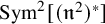
1. We have that Z is the total space of the G-equivariant vector bundle $\mathfrak {n}^2$
, and
$\mathfrak {n}^{\ast } \cong \mathfrak {g}/\mathfrak {b}$
. Therefore $$\begin{align*}Z=\underline{\operatorname{Spec}}_{F}(\operatorname{Sym}[(\mathfrak{g}/\mathfrak{b})^2]),\end{align*}$$and the result follows.
-
2. Recall that $\omega _Z\cong \omega _{Z/F}\otimes _{\mathcal {O}_Z} \pi _Z^{\ast }\omega _F$
because
$\pi _Z$
and F are smooth. We also recall from [Reference Jantzen14] II. §4.2 that
$\omega _F\cong \mathcal {O}(-2\rho )$
. It remains to calculate
$\omega _{Z/F}$
. Notice that the relative tangent bundle has
$T_{Z/F}=\pi _Z^{\ast }((\mathfrak {n})^2)$
, so
$\omega _{Z/F}\cong \pi _Z^{\ast }\det ((\mathfrak {g}/\mathfrak {b})^2)=\pi _Z^{\ast }(\mathcal {O}(4\rho ))$
. Therefore $$\begin{align*}\omega_Z\cong \pi_Z^{\ast}(\mathcal{O}(-2\rho)\otimes\mathcal{O}(4\rho))=\pi_Z^{\ast}(\mathcal{O}(2\rho)) = \mathcal{O}_Z(2\rho).\end{align*}$$
-
3. Write a general point of $\mathfrak {n}^2$
as $$\begin{align*}(M, N) = \left(\begin{pmatrix} 0 & a & b \\ 0 & 0 & c \\ 0 & 0 & 0 \end{pmatrix},\begin{pmatrix} 0 & d & e \\ 0 & 0 & f \\ 0 & 0 & 0 \end{pmatrix}\right)\end{align*}$$as in Lemma 2.3. Then $a, b, \ldots , f$
are a basis for
$(\mathfrak {n}^2)^{\ast }$
. The ideal sheaf of
$C(\mathfrak {n})$
inside
$\operatorname {Sym}[(\mathfrak {n}^2)^{\ast }]$
is principal, generated by
$af - dc$
, which is an element of
$\operatorname {Sym}^2[(\mathfrak {n}^2)^{\ast }]$
of weight
$\rho $
.Footnote 1 In other words, $$\begin{align*}\mathcal{I}_{C(\mathfrak{n})} \cong \mathcal{O}_{\mathfrak{n} \times \mathfrak{n}}(\rho)\end{align*}$$as B-equivariant sheaves on $\mathfrak {n}^2$
. Since
$Y = G\times ^B C(\mathfrak {n})\subset G \times ^B\mathfrak {n}^2 = Z$
we get that $$\begin{align*}\mathcal{I}_Y \cong \mathcal{O}_Z(\rho)\end{align*}$$as required.
-
4. This follows from the adjunction formula (see [22, Section 0AU3 (7)])
$$\begin{align*}\omega_Y = i^{\ast}(\omega_Z\otimes_{\mathcal{O}_Z} \mathcal{I}_Y^\vee)\end{align*}$$and parts (2) and (3).















3.3 Proof of Theorem 2.4
We first prove Theorem 2.4 when
$n = 2$
 . This essentially appears (in the context of ordinary deformation rings when
$l = p$
. This essentially appears (in the context of ordinary deformation rings when
$l = p$
 ) in section 3.3 of [Reference Snowden21], but we include the proof here to illustrate the ideas in this setting and to prepare the ground for the more complicated case
$n = 3$
) in section 3.3 of [Reference Snowden21], but we include the proof here to illustrate the ideas in this setting and to prepare the ground for the more complicated case
$n = 3$
 .
.
Proof of Theorem 2.4 when
$n=2$

In this case
$F=\mathbb {P}^1$
 and
$Y=Z$
and
$Y=Z$
 is the total space of the vector bundle
$\mathfrak {n}^2$
is the total space of the vector bundle
$\mathfrak {n}^2$
 . As line bundles on
$\mathbb {P}^1$
. As line bundles on
$\mathbb {P}^1$
 , we see that

and
$\mathcal {O}(\rho )\cong \mathcal {O}(1)$
 , so that

for every
$r\geq 0$
 . By Proposition 3.2,

and

Since X is affine,
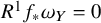
$H^1(Y,\mathcal {O}_Y) = H^0(X, R^1f_{\ast }\mathcal {O}_Y)$
 vanishes and so

Similarly,
$R^1f_{\ast }\omega _Y= 0$
 .
.
It remains to show that
$f^{\ast }:H^0(X,\mathcal {O}_X)\hookrightarrow H^0(Y,\mathcal {O}_Y)$
 is an isomorphism. For convenience, we set
$R=H^0(X,\mathcal {O}_X)$
is an isomorphism. For convenience, we set
$R=H^0(X,\mathcal {O}_X)$
 and
$\tilde {R}=H^0(Y,\mathcal {O}_Y)$
and
$\tilde {R}=H^0(Y,\mathcal {O}_Y)$
 . We note that the natural map

is surjective because X is defined as a closed subscheme of
$\mathfrak {g}^2$
 (and recall that we are identifying
$\mathfrak {g} \cong \mathfrak {g}^{\ast }$
(and recall that we are identifying
$\mathfrak {g} \cong \mathfrak {g}^{\ast }$
 via the trace pairing). Let I be the kernel of this surjection. The composite

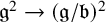
is the morphism induced by the natural surjective map of coherent sheaves
$\mathfrak {g}^2\rightarrow (\mathfrak {g}/\mathfrak {b})^2$
 .
.
Letting
$S=\mathbb {F}[\mathfrak {g}^2]$
 and
$S_+$
and
$S_+$
 be the irrelevant ideal of S, Proposition 2.1.5 of [Reference Snowden21] gives us that

Because of the (nonequivariant) isomorphism of vector bundles
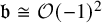
$\mathfrak {b}\cong \mathcal {O}(-1)^2$
 , this shows that
$\tilde {R}/S_+\tilde {R}$
, this shows that
$\tilde {R}/S_+\tilde {R}$
 is
$1$
is
$1$
 -dimensional. Hence the composite
$\mathbb {F}[\mathfrak {g}^2] \rightarrow R \rightarrow \tilde {R}$
-dimensional. Hence the composite
$\mathbb {F}[\mathfrak {g}^2] \rightarrow R \rightarrow \tilde {R}$
 is surjective. It follows that the map
$H^0(X,\mathcal {O}_X)\rightarrow H^0(Y,\mathcal {O}_Y)$
is surjective. It follows that the map
$H^0(X,\mathcal {O}_X)\rightarrow H^0(Y,\mathcal {O}_Y)$
 is an isomorphism as required.
Remark 3.4. The above proof works equally well for the Steinberg component of the fixed-determinant moduli space in the case
$l = 2$
 .
.
Next we turn to the main case of interest for this article,
$n = 3$
 ; we defer the actual cohomological calculations until the next section.
Proof of Theorem 2.4 when
$n=3$

By Proposition 4.15 below,

for all
$i>0$
 . To prove the theorem, the only thing that remains to check is that the natural morphism
$f^{\ast }H^0(X,\mathcal {O}_X)\hookrightarrow H^0(Y,\mathcal {O}_Y)$
. To prove the theorem, the only thing that remains to check is that the natural morphism
$f^{\ast }H^0(X,\mathcal {O}_X)\hookrightarrow H^0(Y,\mathcal {O}_Y)$
 , injective since
$Y \to X$
, injective since
$Y \to X$
 is birational, is an isomorphism.
As in the case
$n = 2$
 , define
$S=\mathbb {F}[\mathfrak {g}^2]=\operatorname {Sym}[\mathfrak {g}^2]$
, define
$S=\mathbb {F}[\mathfrak {g}^2]=\operatorname {Sym}[\mathfrak {g}^2]$
 , with irrelevant ideal
$S_+$
, with irrelevant ideal
$S_+$
 . Let
$\tilde {R}=H^0(Z,\mathcal {O}_Z)$
. Let
$\tilde {R}=H^0(Z,\mathcal {O}_Z)$
 for Z the total space of the vector bundle
$\mathfrak {n}^2$
for Z the total space of the vector bundle
$\mathfrak {n}^2$
 on
$G/B$
on
$G/B$
 . By Lemma 4.12,
$H^i(Z, \mathcal {O}_Z) = 0$
. By Lemma 4.12,
$H^i(Z, \mathcal {O}_Z) = 0$
 for
$i> 0$
for
$i> 0$
 . We may therefore apply Proposition 2.1.5 of [Reference Snowden21] to deduce that

By Calculation 4.4 below, we know that
$H^i(F,\Lambda ^i[\mathfrak {b}^2])=0$
 unless
$i=0$
unless
$i=0$
 , when

Thus the map
$S\rightarrow \tilde {R}$
 is surjective and, as
$H^1(Z, \mathcal {I}_Y) = 0$
is surjective and, as
$H^1(Z, \mathcal {I}_Y) = 0$
 by Proposition 3.2 and Lemma 4.12, the map
$\tilde {R} = H^0(Z, \mathcal {O}_Z)\rightarrow H^0(Y,\mathcal {O}_Y)$
by Proposition 3.2 and Lemma 4.12, the map
$\tilde {R} = H^0(Z, \mathcal {O}_Z)\rightarrow H^0(Y,\mathcal {O}_Y)$
 is surjective. The composite map

is equal to the composite

and so
$f^{\ast }$
 is surjective as required.
4 Cohomology of sheaves on the flag variety when
$n=3$

We let
$n = 3$
 and
$G = \mathrm {SL}_3$
and
$G = \mathrm {SL}_3$
 , and continue with the notation of section 3.1. Let
$X(T)$
, and continue with the notation of section 3.1. Let
$X(T)$
 be the character lattice,
$X^{\vee }(T)$
be the character lattice,
$X^{\vee }(T)$
 be the cocharacter lattice, and
$\langle \,,\rangle :X(T)\times X^{\vee }(T)\rightarrow \mathbb {Z}$
be the cocharacter lattice, and
$\langle \,,\rangle :X(T)\times X^{\vee }(T)\rightarrow \mathbb {Z}$
 be the natural pairing. For a character
$\lambda \in X(T)$
be the natural pairing. For a character
$\lambda \in X(T)$
 , let
$\mathbb {F}(\lambda )$
, let
$\mathbb {F}(\lambda )$
 be the corresponding representation of B and recall that in Section 3.1 we have defined a line bundle
$\mathcal {O}(\lambda )$
be the corresponding representation of B and recall that in Section 3.1 we have defined a line bundle
$\mathcal {O}(\lambda )$
 on
$G/B$
on
$G/B$
 . We have chosen the system
$\Phi ^+$
. We have chosen the system
$\Phi ^+$
 of positive roots such that the weights of
$\mathfrak {n}$
of positive roots such that the weights of
$\mathfrak {n}$
 are negative. Our basic tool will be the Borel–Weil–Bott theorem, which holds in positive characteristic for ‘sufficiently small’ weights.
Let

and
$C^0_{\mathbb {Z}} = \overline {C}_{\mathbb {Z}} \cap X(T)_+$
 . Recall the ‘dot action’ of the Weyl group
$W \cong S_3$
. Recall the ‘dot action’ of the Weyl group
$W \cong S_3$
 of G on
$X(T)$
of G on
$X(T)$
 :
:

Theorem 4.1. Let
$\lambda \in \overline {C}_{\mathbb {Z}}$
 .
.
-
1. If $\lambda \in C^0_{\mathbb {Z}}$
then
$H^0(G/B, \mathcal {O}(\lambda ))$
is an irreducible representation of G that we denote by
$V(\lambda )$
. -
2. The representations $V(\lambda )$
for
$\lambda \in C^0_{\mathbb {Z}}$
are pairwise nonisomorphic. -
3. If $\lambda \not \in C^0_{\mathbb {Z}}$
, then
$H^i(G/B, \mathcal {O}(\lambda )) = 0$
for all i. -
4. If $w\in W$
, then
$H^i(G/B,\mathcal {O}(w\cdotp \lambda ))=0$
unless
$i=l(w)$
, in which case $$\begin{align*}H^{l(w)}(G/B,\mathcal{O}(w\cdotp\lambda))\cong H^0(G/B,\mathcal{O}(\lambda)).\end{align*}$$









Proof. This is Corollary II.5.5 and Corollary II.5.6 of [Reference Jantzen14].
In what follows, for V a representation of B, we will abbreviate
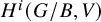
$H^i(G/B, V)$
 to
$H^i(V)$
to
$H^i(V)$
 . For V a representation of B and
$\lambda $
. For V a representation of B and
$\lambda $
 a character of T we write
$V_{\lambda } = \{v \in V : tv =\lambda (v)t \text { for all } t \in T\}$
a character of T we write
$V_{\lambda } = \{v \in V : tv =\lambda (v)t \text { for all } t \in T\}$
 for the
$\lambda $
for the
$\lambda $
 -weight space of V. The multiset in which each character
$\lambda $
-weight space of V. The multiset in which each character
$\lambda $
 of T occurs
$\dim (V_{\lambda })$
of T occurs
$\dim (V_{\lambda })$
 times is the multiset of weights of V; its elements are the weights of V.
We will call
$\bigcup _{w \in W} w \cdot \overline {C}_{\mathbb {Z}}$
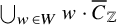 the BWB locus and say that a representation V of B is BWB-good if all of its weights are in the BWB locus. For
$i\ge 0$
the BWB locus and say that a representation V of B is BWB-good if all of its weights are in the BWB locus. For
$i\ge 0$
 let
$C^i_{\mathbb {Z}}=\coprod _{l(w)=i}w\cdotp C^0_{\mathbb {Z}}$
let
$C^i_{\mathbb {Z}}=\coprod _{l(w)=i}w\cdotp C^0_{\mathbb {Z}}$
 . For
$i \ge 0$
. For
$i \ge 0$
 and V a BWB-good representation of B, we let

viewed as a multiset where the multiplicity of
$\lambda $
 is the sum of the multiplicities of
$w\cdot \lambda $
is the sum of the multiplicities of
$w\cdot \lambda $
 as weights of V.
Lemma 4.2. Suppose that V is a BWB-good representation of B and
$i \ge 0$
 .
.
-
1. The G-representation $H^i(V)$
has a composition series in which all irreducible subquotients have the form
$V(\lambda )$
for
$\lambda \in \operatorname {psupp}^i(V)$
, and each
$V(\lambda )$
occurs with multiplicity at most the multiplicity of
$\lambda $
in
$\operatorname {psupp}^i(V)$
. -
2. The representation $H^i(V)$
is completely reducible.





Proof. Part (1) results from repeatedly applying the long exact sequence in cohomology to a composition series for V. By [Reference Jantzen14, Proposition II.4.13],

for all
$\lambda , \mu \in C^0_{\mathbb {Z}}$
 and
$i> 0$
and
$i> 0$
 . Part (2) follows from this and part (1).
If V is a representation of B then we let

where the sum is taken in the Grothendieck group of the category of finite-dimensional representations of G. Formation of
$\chi $
 is additive in short exact sequences, and we therefore have

for a BWB-good representation V of B.
Finally, we will also need the fact (see [Reference Jantzen14, Proposition I.4.8]) that, if V is a B-representation and W a G-representation, then
$H^i(V\otimes W)\cong H^i(V)\otimes W$
 as G-representations for all
$i\ge 0$
as G-representations for all
$i\ge 0$
 .
.
We let
$L_1, L_2, L_3 \in X(T)$
 be the characters taking
$t \in T$
be the characters taking
$t \in T$
 to its respective diagonal entries, labelled so that
$L_1$
to its respective diagonal entries, labelled so that
$L_1$
 corresponds to the bottom right entry (!) and
$L_3$
corresponds to the bottom right entry (!) and
$L_3$
 to the top left. Then
$L_1$
to the top left. Then
$L_1$
 and
$-L_3$
and
$-L_3$
 generate the monoid
$X(T)_+$
generate the monoid
$X(T)_+$
 of dominant weights and we have
$\rho = L_1 - L_3$
of dominant weights and we have
$\rho = L_1 - L_3$
 . The positive simple roots are
$\alpha = L_1 - L_2$
. The positive simple roots are
$\alpha = L_1 - L_2$
 and
$\beta = L_2 - L_3$
and
$\beta = L_2 - L_3$
 . The lines
$\{\mu : \left \langle \mu + \rho , \kappa ^\vee \right \rangle = 0\}$
. The lines
$\{\mu : \left \langle \mu + \rho , \kappa ^\vee \right \rangle = 0\}$
 for
$\kappa \in \{\alpha , \rho , \beta \}$
for
$\kappa \in \{\alpha , \rho , \beta \}$
 divide
$X(T)\otimes \mathbb {R}$
divide
$X(T)\otimes \mathbb {R}$
 into six regions. The weights strictly in the interior of each region are
$w \cdot X(T)_+$
into six regions. The weights strictly in the interior of each region are
$w \cdot X(T)_+$
 for some
$w \in W$
for some
$w \in W$
 . Figure 1 shows the BWB-locus when
$p=5$
. Figure 1 shows the BWB-locus when
$p=5$
 – the interior and boundary of blue dashed region – and shows the different
$C^i_{\mathbb {Z}}$
– the interior and boundary of blue dashed region – and shows the different
$C^i_{\mathbb {Z}}$
 . Also shown are the weights
$L_1,L_2,L_3$
. Also shown are the weights
$L_1,L_2,L_3$
 ,
$\alpha ,\beta ,\rho ,-\rho $
,
$\alpha ,\beta ,\rho ,-\rho $
 , and
$-2\rho $
, and
$-2\rho $
 ; the weights of
$\mathfrak {b}$
; the weights of
$\mathfrak {b}$
 are coloured red and those of
$\mathfrak {g}/\mathfrak {b}$
are coloured red and those of
$\mathfrak {g}/\mathfrak {b}$
 coloured green.
The weight lattice of
$SL_3$
 .
.

Figure 1 Long description
A coordinate system with three intersecting gray lines labeled L sub 1, L sub 2, and L sub 3 meeting at a central red dot labeled minus rho. A grid of black dots forms a hexagonal lattice across the background.
At the center right, a red circle with a white dot inside is labeled 0. To its right, a light blue shaded triangle is labeled C sub Z super 0. Inside this triangle is a green dot labeled rho.
Moving clockwise around the center
- In the bottom right sector, a blue triangle is labeled C sub Z super 1. A green dot on the L sub 2 axis is labeled beta.
- In the bottom left sector, a blue triangle is labeled C sub Z super 2.
- On the far left, a blue triangle is labeled C sub Z super 3, with its inner vertex labeled minus 2 rho.
- In the top left sector, a blue triangle is labeled C sub Z super 2.
- In the top right sector, a blue triangle is labeled C sub Z super 1. A green dot on the L sub 3 axis is labeled alpha.
A dashed blue hexagonal perimeter encloses these six triangular regions. Additional red dots are positioned at the inner vertices of the top and bottom right triangles.
4.0.1 Calculating
$H^i(\Lambda ^j[\mathfrak {b}\oplus \mathfrak {b}])$

Calculation 4.3. Suppose that
$l \ge 5$
 . Then the G-representations
$H^i(\Lambda ^j\mathfrak {b})$
. Then the G-representations
$H^i(\Lambda ^j\mathfrak {b})$
 are as shown in Table 1. Moreover,
$H^i(\mathfrak {b} \otimes \mathfrak {b}) = H^i(\Lambda ^2\mathfrak {b})$
are as shown in Table 1. Moreover,
$H^i(\mathfrak {b} \otimes \mathfrak {b}) = H^i(\Lambda ^2\mathfrak {b})$
 for all i.
The cohomology groups
$H^i(\Lambda ^j\mathfrak {b})$
 .
.

Table 1 Long description
The table is organized with columns labeled by the index i (0, 1, 2, 3) and rows labeled by the index j (0, 1, 2, 3, 4, 5). The top-left header cell contains j backslash i.
* Row j equals 0: Column i equals 0 contains blackboard bold F. Columns i equals 1, 2, and 3 contain a centered dot.
* Row j equals 1: All columns (i equals 0, 1, 2, 3) contain a centered dot.
* Row j equals 2: Column i equals 1 contains blackboard bold F. Columns i equals 0, 2, and 3 contain a centered dot.
* Row j equals 3: Column i equals 2 contains blackboard bold F. Columns i equals 0, 1, and 3 contain a centered dot.
* Row j equals 4: All columns (i equals 0, 1, 2, 3) contain a centered dot.
* Row j equals 5: Column i equals 3 contains blackboard bold F. Columns i equals 0, 1, and 2 contain a centered dot.
Proof. If
$l \ge 5$
 then each of the representations
$\mathfrak {b}$
then each of the representations
$\mathfrak {b}$
 ,
$\mathfrak {g}/\mathfrak {b}$
,
$\mathfrak {g}/\mathfrak {b}$
 ,
$\mathfrak {b} \otimes \mathfrak {b}$
,
$\mathfrak {b} \otimes \mathfrak {b}$
 , and
$\mathfrak {b} \otimes \mathfrak {g}/\mathfrak {b}$
, and
$\mathfrak {b} \otimes \mathfrak {g}/\mathfrak {b}$
 is BWB-good. We may therefore discuss the potential support of these representations and apply Lemma 4.2 to them.
-
0. When $j=0$
,
$\Lambda ^j\mathfrak {b}=\mathbb {F}$
. By Theorem 4.1,
$H^i(\mathbb {F})=0$
unless
$i=0$
, in which case
$H^0(\mathbb {F})=\mathbb {F}$
. -
1. When $j=1$
, we note that
$\operatorname {psupp}^2(\mathfrak {b})=\operatorname {psupp}^3(\mathfrak {b})=\emptyset $
, so $$\begin{align*}H^2(\mathfrak{b})=H^3(\mathfrak{b})=0.\end{align*}$$We have
$$\begin{align*}\operatorname{psupp}^0(\mathfrak{b}) = \operatorname{psupp}^1(\mathfrak{b}) = \{0, 0\}\end{align*}$$and so all composition factors of $H^0(\mathfrak {b})$
and
$H^1(\mathfrak {b})$
are trivial as G-representations.
Further, there is a short exact sequence
$$\begin{align*}0\rightarrow\mathfrak{b}\to \mathfrak{g}\to \mathfrak{g}/\mathfrak{b}\to 0\end{align*}$$which gives a long exact sequence in cohomology
As $\mathfrak {g}$
is a G-representation, we see from part (0) that
$H^0(\mathfrak {g})=\mathfrak {g}$
and
$H^1(\mathfrak {g})=0$
. For
$\mathfrak {g}/\mathfrak {b}$
we have
$\operatorname {psupp}^0(\mathfrak {g}/\mathfrak {b})=\{\rho \}$
and
$\operatorname {psupp}^i(\mathfrak {g}/\mathfrak {b}) = 0$
for
$i> 0$
. Thus
$H^0(\mathfrak {g}/\mathfrak {b})\subset V(\rho ) = \mathfrak {g}$
. As all subquotients of
$H^0(\mathfrak {b})$
and
$H^1(\mathfrak {b})$
are the trivial representation, we must have
$H^0(\mathfrak {b}) = H^1(\mathfrak {b}) = 0$
and
$H^0(\mathfrak {g}/\mathfrak {b}) = \mathfrak {g}$
.
-
2. When $j=2$
, consider the exact sequence $$\begin{align*}0\rightarrow\mathfrak{b}\otimes\mathfrak{b}\to \mathfrak{g}\otimes\mathfrak{b}\to \mathfrak{g}/\mathfrak{b}\otimes\mathfrak{b}\to 0,\end{align*}$$from which we get a long exact sequence with parts
$$\begin{align*}H^i(\mathfrak{g}\otimes\mathfrak{b})\to H^i(\mathfrak{g}/\mathfrak{b}\otimes\mathfrak{b})\to H^{i+1}(\mathfrak{b}\otimes\mathfrak{b})\to H^{i+1}(\mathfrak{g}\otimes\mathfrak{b}).\end{align*}$$As $H^i(\mathfrak {b})=0$
for all i, we obtain isomorphisms
$H^i(\mathfrak {b}\otimes \mathfrak {g}/\mathfrak {b})\cong H^{i+1}(\mathfrak {b}\otimes \mathfrak {b})$
for all i. Thus,
$H^0(\mathfrak {b}\otimes \mathfrak {b})=0$
and
$H^3(\mathfrak {b}\otimes \mathfrak {b})=H^2(\mathfrak {g}/\mathfrak {b}\otimes \mathfrak {b})=0$
, since
$\operatorname {psupp}^2(\mathfrak {g}/\mathfrak {b}\otimes \mathfrak {b})=\emptyset $
.
To show that $H^2(\mathfrak {b}\otimes \mathfrak {b}) = 0$
, consider first the exact sequence $$\begin{align*}0\rightarrow\mathfrak{b}\otimes\mathfrak{g}/\mathfrak{b}\to \mathfrak{g}\otimes\mathfrak{g}/\mathfrak{b}\to \mathfrak{g}/\mathfrak{b}\otimes\mathfrak{g}/\mathfrak{b}\to 0\end{align*}$$giving rise to the long exact sequence
$$\begin{align*}0\to H^0(\mathfrak{b}\otimes\mathfrak{g}/\mathfrak{b})\to \mathfrak{g} \otimes \mathfrak{g}\to H^{0}(\mathfrak{g}/\mathfrak{b}\otimes\mathfrak{g}/\mathfrak{b})\to H^{1}(\mathfrak{b}\otimes\mathfrak{g}/\mathfrak{b})\to 0.\end{align*}$$Here we have used that $H^1(\mathfrak {g}\otimes \mathfrak {g}/\mathfrak {b})\cong \mathfrak {g} \otimes H^1(\mathfrak {g}/\mathfrak {b})=0$
, as
$\operatorname {psupp}^1(\mathfrak {g}/\mathfrak {b}) = \emptyset $
, and
$H^0(\mathfrak {g}\otimes \mathfrak {g}/\mathfrak {b})\cong \mathfrak {g} \otimes H^0(\mathfrak {g}/\mathfrak {b})\cong \mathfrak {g}\otimes \mathfrak {g}$
. Thus $$\begin{align*}H^2(\mathfrak{b} \otimes \mathfrak{b}) \cong H^1(\mathfrak{b}\otimes \mathfrak{g}/\mathfrak{b})\cong\operatorname{coker}(\mathfrak{g}\otimes\mathfrak{g}\to H^0(\mathfrak{g}/\mathfrak{b}\otimes \mathfrak{g}/\mathfrak{b})).\end{align*}$$Since $\operatorname {psupp}^2(\mathfrak {b} \otimes \mathfrak {b}) = \{0,0,0,0\}$
, every irreducible constituent of
$H^2(\mathfrak {b}\otimes \mathfrak {b})$
is trivial. So it is enough to show that
$H^0(\mathfrak {g}/\mathfrak {b}\otimes \mathfrak {g}/\mathfrak {b})$
does not have the trivial representation as a subquotient. If
$l \ge 7$
, this follows as
$\mathfrak {g}/\mathfrak {b} \otimes \mathfrak {g}/\mathfrak {b}$
is BWB-good and
$0 \not \in \operatorname {psupp}^0(\mathfrak {b} \otimes \mathfrak {g}/\mathfrak {b})$
. If
$l = 5$
then every weight of
$\mathfrak {g}/\mathfrak {b} \otimes \mathfrak {g}/\mathfrak {b}$
except for
$2\rho $
is in the BWB locus and nonzero, so cannot give rise to a trivial subquotient of
$H^0(\mathfrak {g}/\mathfrak {b} \otimes \mathfrak {g}/\mathfrak {b})$
. Every other composition factor of
$H^0(\mathfrak {g}/\mathfrak {b}\otimes \mathfrak {g}/\mathfrak {b})$
is isomorphic to a composition factor of
$H^0(\mathbb {F}(2\rho ))$
. By the strong linkage principle of [Reference Jantzen14, Proposition II.6.13], these are of the form
$V(\rho )$
or
$L(2\rho )$
(the irreducible representation with highest weight
$2\rho $
), and are therefore nontrivial as required.
Finally, we compute
$$\begin{align*}\chi(\mathfrak{b}\otimes\mathfrak{b})=4[\mathbb{F}]-4[\mathbb{F}]-4[\mathbb{F}]+2[\mathbb{F}]+2[\mathbb{F}]-[\mathbb{F}]=-[\mathbb{F}].\end{align*}$$Since $H^i(\mathfrak {b}\otimes \mathfrak {b}) = 0$
for
$i \ne 1$
, we deduce that
$H^1(\mathfrak {b}\otimes \mathfrak {b})=\mathbb {F}$
. As
$\Lambda ^2\mathfrak {b}$
is a direct summand of
$\mathfrak {b}\otimes \mathfrak {b}$
(as
$l> 2$
), it follows that
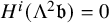
$H^i(\Lambda ^2\mathfrak {b})=0$
when
$i\neq 1$
and, as $$\begin{align*}\chi(\Lambda^2\mathfrak{b})=[\mathbb{F}]-4[\mathbb{F}]+2[\mathbb{F}]=-[\mathbb{F}],\end{align*}$$$H^1(\Lambda ^2\mathfrak {b})= \mathbb {F} = H^1(\mathfrak {b} \otimes \mathfrak {b})$
.
For later use, also note that we have shown $H^i(\mathfrak {b} \otimes \mathfrak {g}/\mathfrak {b}) = 0$
for
$i> 0$
; an Euler characteristic calculation then shows that
$H^0(\mathfrak {b} \otimes \mathfrak {g}/\mathfrak {b}) = \mathbb {F}$
. -
3. For $j = 3, 4, 5$
we have a B-equivariant pairing $$\begin{align*}\Lambda^j\mathfrak{b} \times \Lambda^{5-j}\mathfrak{b} \to \Lambda^5 \mathfrak{b} \cong \mathbb{F}(-2\rho)\end{align*}$$and so
$$\begin{align*}(\Lambda^j\mathfrak{b})^{\ast} \otimes \mathbb{F}(-2\rho) \cong \Lambda^{5-j}\mathfrak{b}.\end{align*}$$Since $\omega _{G/B} \cong \mathbb {F}(-2\rho )$
, Serre duality gives $$\begin{align*}H^i(\Lambda^j\mathfrak{b}) \cong H^{3-i}(\Lambda^{5-j}\mathfrak{b})^{\ast}\end{align*}$$and the result follows from parts 0–2.












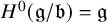








































Calculation 4.4. Suppose that
$l \geq 5$
 . Then

Proof. Firstly, we observe that
$\mathfrak {b}\otimes \mathfrak {b} \otimes \mathfrak {g}$
 , and therefore any subquotient of it, is BWB-good for
$l \ge 5$
, and therefore any subquotient of it, is BWB-good for
$l \ge 5$
 . This justifies the use of potential supports in the following calculation.
Considering the long exact sequence associated to

along with the isomorphism
$H^i(\mathfrak {g}\otimes \Lambda ^2\mathfrak {b})=\mathfrak {g}\otimes H^i(\Lambda ^2\mathfrak {b})$
 and the results of Calculation 4.3, we obtain an exact sequence

an isomorphism

and
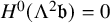
$H^0(\Lambda ^2\mathfrak {b}\otimes \mathfrak {b})=0$
 . As
$\operatorname {psupp}^2(\Lambda ^2\mathfrak {b}\otimes \mathfrak {g}/\mathfrak {b})=\emptyset $
. As
$\operatorname {psupp}^2(\Lambda ^2\mathfrak {b}\otimes \mathfrak {g}/\mathfrak {b})=\emptyset $
 , we see that
$H^3(\Lambda ^2\mathfrak {b}\otimes \mathfrak {b})=0$
, we see that
$H^3(\Lambda ^2\mathfrak {b}\otimes \mathfrak {b})=0$
 .
.
We calculate (using superscripts to denote multiplicity)

and so

Since
$\rho $
 appears only in
$\operatorname {psupp}^2$
appears only in
$\operatorname {psupp}^2$
 , we obtain that

and

for some integer
$n \ge 0$
 . It follows that

since the map
$H^1(\Lambda ^2\mathfrak {b}\otimes \mathfrak {b})\to \mathfrak {g}$
 must be zero.
The B-representation
$\Lambda ^2\mathfrak {b}\otimes \mathfrak {g}/\mathfrak {b}$
 is a direct summand of
$\mathfrak {b}\otimes \mathfrak {b}\otimes \mathfrak {g}/\mathfrak {b}$
is a direct summand of
$\mathfrak {b}\otimes \mathfrak {b}\otimes \mathfrak {g}/\mathfrak {b}$
 , which fits into the short exact sequence

and so we have an exact sequence

(the last isomorphism appearing in part 2 of the proof of Calculation 4.3). As
$H^0(\Lambda ^2\mathfrak {b}\otimes \mathfrak {g}/\mathfrak {b})\cong \mathbb {F}^n$
 and
$\mathbb {F}$
and
$\mathbb {F}$
 is not a subrepresentation of
$\mathfrak {g}$
is not a subrepresentation of
$\mathfrak {g}$
 , we deduce that
$H^0(\Lambda ^2\mathfrak {b}\otimes \mathfrak {g}/\mathfrak {b})=H^1(\Lambda ^2\mathfrak {b}\otimes \mathfrak {b})=0$
, we deduce that
$H^0(\Lambda ^2\mathfrak {b}\otimes \mathfrak {g}/\mathfrak {b})=H^1(\Lambda ^2\mathfrak {b}\otimes \mathfrak {b})=0$
 .
.
Calculation 4.5.
-
1. Suppose that $l \ge 5$
. Then $$\begin{align*}H^3(\Lambda^3\mathfrak{b} \otimes \mathfrak{b}) = 0.\end{align*}$$
-
2. Suppose that $l \ge 5$
. Then $$\begin{align*}H^3(\Lambda^2 \mathfrak{b} \otimes \Lambda^2 \mathfrak{b}) = 0.\end{align*}$$


Proof.
-
1. We first show that $H^3(\Lambda ^3\mathfrak {b} \otimes \mathfrak {b}) = 0$
. By Serre duality, the pairing
$\Lambda ^3 \mathfrak {b} \times \Lambda ^2\mathfrak {b} \to \Lambda ^5\mathfrak {b} \cong \mathbb {F}(-2\rho )$
, and the isomorphism
$\omega _F \cong \mathcal {O}_F(-2\rho )$
, we have $$\begin{align*}H^3(\Lambda^3\mathfrak{b} \otimes \mathfrak{b}) \cong H^0(\Lambda^2\mathfrak{b} \otimes \mathfrak{b}^{\ast})^{\ast}.\end{align*}$$Since $\mathfrak {b}^{\ast } \cong \mathfrak {g}/\mathfrak {n}$
, we wish to show that
$H^0(\Lambda ^2\mathfrak {b} \otimes \mathfrak {g}/\mathfrak {n}) = 0$
. The last line of the proof of Calculation 4.4 shows that
$H^0(\Lambda ^2\mathfrak {b} \otimes \mathfrak {g}/\mathfrak {b}) = 0$
, and by Calculation 4.3
$H^0(\Lambda ^2\mathfrak {b}) = 0$
. The result follows by tensoring the short exact sequence of B-representations $$\begin{align*}0 \to \mathfrak{b}/\mathfrak{n} \cong \mathbb{F}^2 \to \mathfrak{g}/\mathfrak{n} \to \mathfrak{g}/\mathfrak{b} \to 0\end{align*}$$with $\Lambda ^2\mathfrak {b}$
and applying
$H^0(\cdot )$
.
-
2. If $l\geq 5$
then
$\Lambda ^2\mathfrak {b} \otimes \Lambda ^2\mathfrak {b}$
is BWB-good, which justifies the following argument in characteristic l. Note that the only weights in
$\operatorname {psupp}^3(\Lambda ^2\mathfrak {b} \otimes \Lambda ^2\mathfrak {b})$
are
$0$
and
$\rho $
, so that
$H^3(\Lambda ^2\mathfrak {b} \otimes \Lambda ^2\mathfrak {b})$
is a direct sum of copies of
$\mathbb {F}$
and
$\mathfrak {g}$
.Let $e_{\pm \alpha }$
,
$e_{\pm \rho }$
and
$e_{\pm \beta }$
be root vectors in
$\mathfrak {g}$
(chosen to be elementary matrices) and let P be the parabolic subgroup of G whose Lie algebra is spanned by
$\mathfrak {b}$
and
$e_{\alpha }$
, with unipotent radical
$U_P$
and Levi quotient
$M = P/U_P \cong GL_2$
. We will use the following lemma of Demazure.
















Lemma 4.6 (‘Easy Lemma’ of [Reference Demazure6])
If V is a representation of B and
$\lambda \in X(T)$
 is such that
$\left \langle \lambda , \alpha ^\vee \right \rangle = 1$
is such that
$\left \langle \lambda , \alpha ^\vee \right \rangle = 1$
 , and if
$V(\lambda )$
, and if
$V(\lambda )$
 extends to a representation of P, then
$H^i(V) = 0$
extends to a representation of P, then
$H^i(V) = 0$
 for all
$i \ge 0$
for all
$i \ge 0$
 .
.
The next lemma allows us to recognize certain representations that extend to P.
Lemma 4.7. Suppose that V is a representation of B such that:
-
• $\dim (V) \le l$
-
• $e_{-\beta }$
and
$e_{-\rho }$
act as zero on V; -
• There is a vector $v \in V$
of weight
$\mu $
such that
$\left \langle \mu , \alpha \right \rangle = \dim (V) - 1$
and such that $$\begin{align*}v, e_{-\alpha}v, \ldots, e_{-\alpha}^{\dim(V) -1}v\end{align*}$$is a basis of V.




Then V extends to a representation of P.
Proof. Since
$e_{-\beta }$
 and
$e_{-\rho }$
and
$e_{-\rho }$
 act as zero on V and
$\dim (V) \le l$
act as zero on V and
$\dim (V) \le l$
 , the root subgroups
$U_{-\beta }$
, the root subgroups
$U_{-\beta }$
 and
$U_{-\rho }$
and
$U_{-\rho }$
 act trivially on V, and therefore so does
$U_P$
act trivially on V, and therefore so does
$U_P$
 . Thus the action of B factors through the quotient
$B \to B/U_P$
. Thus the action of B factors through the quotient
$B \to B/U_P$
 . The third condition, together with the restriction
$\dim (V) \le l$
. The third condition, together with the restriction
$\dim (V) \le l$
 , implies that V is the restriction to
$B/U_P$
, implies that V is the restriction to
$B/U_P$
 of an irreducible representation of
$M \cong GL_2$
of an irreducible representation of
$M \cong GL_2$
 whose restriction to
$M^{\mathrm {der}} \cong SL_2$
whose restriction to
$M^{\mathrm {der}} \cong SL_2$
 is the irreducible representation of highest weight
$\dim (V)-1$
is the irreducible representation of highest weight
$\dim (V)-1$
 . In particular, V extends to P.
We first show that
$H^3(\Lambda ^2\mathfrak {b} \otimes \Lambda ^2\mathfrak {b})$
 does not contain the trivial representation. Let
$V_1 \subset \Lambda ^2\mathfrak {b} \otimes \Lambda ^2\mathfrak {b}$
does not contain the trivial representation. Let
$V_1 \subset \Lambda ^2\mathfrak {b} \otimes \Lambda ^2\mathfrak {b}$
 be the
$\mathbb {F}$
be the
$\mathbb {F}$
 -span of all weight vectors of weights in

and let
$V_2$
 be the
$\mathbb {F}$
be the
$\mathbb {F}$
 -span of
$V_1$
-span of
$V_1$
 and all weight vectors of weights in
$\{-2\rho , -\rho - \alpha , -\rho -\beta \}$
and all weight vectors of weights in
$\{-2\rho , -\rho - \alpha , -\rho -\beta \}$
 . Then
$V_1$
. Then
$V_1$
 and
$V_2$
and
$V_2$
 are B-subrepresentations of
$V_3 = \Lambda ^2\mathfrak {b} \otimes \Lambda ^2\mathfrak {b}$
are B-subrepresentations of
$V_3 = \Lambda ^2\mathfrak {b} \otimes \Lambda ^2\mathfrak {b}$
 . Let
$V = V_2/V_1$
. Let
$V = V_2/V_1$
 . Because
$0$
. Because
$0$
 is not contained in
$\operatorname {psupp}^3(V_1)$
is not contained in
$\operatorname {psupp}^3(V_1)$
 or
$\operatorname {psupp}^3(V3/V_2)$
or
$\operatorname {psupp}^3(V3/V_2)$
 , to show that
$H^3(V_3)$
, to show that
$H^3(V_3)$
 contains no copy of the trivial representation it is enough to show that
$H^3(V) = 0$
contains no copy of the trivial representation it is enough to show that
$H^3(V) = 0$
 .
.
Consider the weight space
$V_{-\rho -\beta }\subseteq V$
 . The B-representation generated by
$V_{\rho -\beta }$
. The B-representation generated by
$V_{\rho -\beta }$
 is
$V^{\beta }:=V_{-\rho -\beta }\oplus e_{-\alpha }(V_{-\rho -\beta })$
is
$V^{\beta }:=V_{-\rho -\beta }\oplus e_{-\alpha }(V_{-\rho -\beta })$
 , and this representation splits as a direct sum into copies of
$\mathbb {F}(-\rho -\beta )$
, and this representation splits as a direct sum into copies of
$\mathbb {F}(-\rho -\beta )$
 and
$2$
and
$2$
 -dimensional representations satisfying the hypotheses of Lemma 4.7. Thus,
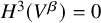
$H^3(V^{\beta })=0$
-dimensional representations satisfying the hypotheses of Lemma 4.7. Thus,
$H^3(V^{\beta })=0$
 by Lemma 4.6. Analogously, consider the B-subrepresentation
$V^{\alpha }\subseteq V/V^{\beta }$
by Lemma 4.6. Analogously, consider the B-subrepresentation
$V^{\alpha }\subseteq V/V^{\beta }$
 generated by
$V_{-\rho -\alpha }$
generated by
$V_{-\rho -\alpha }$
 . In the exact same way (switching the roles of
$\alpha $
. In the exact same way (switching the roles of
$\alpha $
 and
$\beta $
and
$\beta $
 in Lemmas 4.6 and 4.7), we see that
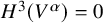
$H^3(V^{\alpha })=0$
in Lemmas 4.6 and 4.7), we see that
$H^3(V^{\alpha })=0$
 . To show that
$H^3(V)=0$
. To show that
$H^3(V)=0$
 , it remains simply to show that
$V^{\alpha }=V/V^{\beta }$
, it remains simply to show that
$V^{\alpha }=V/V^{\beta }$
 , or equivalently, that
$V_{-2\rho }=e_{-\alpha }(V_{-\rho -\beta })+e_{-\beta }(V_{-\rho -\alpha })$
, or equivalently, that
$V_{-2\rho }=e_{-\alpha }(V_{-\rho -\beta })+e_{-\beta }(V_{-\rho -\alpha })$
 .
.
This can be shown via a direct calculation by showing that each of the
$17$
 simple tensors which span
$V_{-2\rho }$
simple tensors which span
$V_{-2\rho }$
 are in this joint image. We outline this calculation. Set
$f_{\gamma }=e_{-\gamma }\in \mathfrak {b}$
are in this joint image. We outline this calculation. Set
$f_{\gamma }=e_{-\gamma }\in \mathfrak {b}$
 (reserving
$e_{-\gamma }=[f_{\gamma },\_]$
(reserving
$e_{-\gamma }=[f_{\gamma },\_]$
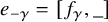 for the linear map) and set
$t_{\alpha },t_{\beta }\in \mathfrak {t}$
for the linear map) and set
$t_{\alpha },t_{\beta }\in \mathfrak {t}$
 a basis of weight
$0$
a basis of weight
$0$
 vectors such that
$e_{-\nu }(t_{\mu })=\delta _{\nu ,\mu }f_{\nu }$
vectors such that
$e_{-\nu }(t_{\mu })=\delta _{\nu ,\mu }f_{\nu }$
 in
$\mathfrak {b}$
in
$\mathfrak {b}$
 for
$\nu ,\mu \in \{\alpha ,\beta \}$
for
$\nu ,\mu \in \{\alpha ,\beta \}$
 . (Such a basis exists when the characteristic
$l\neq 3$
. (Such a basis exists when the characteristic
$l\neq 3$
 ). Then

These three equations give us
$12$
 linearly independent basis elements in the image when we consider the two independent symmetries of swapping the left and right sides of the tensor, and the symmetry interchanging
$e_{-\alpha }$
linearly independent basis elements in the image when we consider the two independent symmetries of swapping the left and right sides of the tensor, and the symmetry interchanging
$e_{-\alpha }$
 and
$-e_{-\beta }$
and
$-e_{-\beta }$
 , the effect of which is to flip the signs of the terms in red. We have further:

again with the two conjugates (swapping
$\alpha \leftrightarrow \beta $
 and flipping the signs of the terms in red) giving us in total
$16$
and flipping the signs of the terms in red) giving us in total
$16$
 of the simple tensor spanning
$V_{-2\rho }$
of the simple tensor spanning
$V_{-2\rho }$
 .
.
The last basis element can be expressed as

with the last two terms inside
$e_{-\alpha }V_{-\rho -\beta }+e_{-\beta }(V_{\rho -\alpha })$
 as previously considered. Since
$V_{-2\rho }$
as previously considered. Since
$V_{-2\rho }$
 is a
$17$
is a
$17$
 dimensional vector space, this shows that
$V_{-2\rho }=e_{-\alpha }(V_{-\rho -\beta })+e_{-\beta }(V_{-\rho -\alpha })$
dimensional vector space, this shows that
$V_{-2\rho }=e_{-\alpha }(V_{-\rho -\beta })+e_{-\beta }(V_{-\rho -\alpha })$
 and, consequently,
${H^3(V)=0}$
and, consequently,
${H^3(V)=0}$
 .
.
We have now shown that
$H^3(\Lambda ^2\mathfrak {b} \otimes \Lambda ^2\mathfrak {b})\cong \mathfrak {g}^s$
 for some
$s \ge 0$
for some
$s \ge 0$
 . The only weight of
$\Lambda ^2\mathfrak {b} \otimes \Lambda ^2\mathfrak {b}$
. The only weight of
$\Lambda ^2\mathfrak {b} \otimes \Lambda ^2\mathfrak {b}$
 remaining that can contribute to
$H^3$
remaining that can contribute to
$H^3$
 is
$-3\rho $
is
$-3\rho $
 , which occurs with multiplicity two; thus
$s \le 2$
, which occurs with multiplicity two; thus
$s \le 2$
 and we wish to show that
$s = 0$
and we wish to show that
$s = 0$
 .
.
Let
$\mu = -2\beta - \rho $
 . In
$\Lambda ^2 \mathfrak {b} \otimes \Lambda ^2\mathfrak {b}$
. In
$\Lambda ^2 \mathfrak {b} \otimes \Lambda ^2\mathfrak {b}$
 let
let

and

Let
$\tilde {W}$
 be the B-representation generated by v, and let
$W = \tilde {W}_{U_P}$
be the B-representation generated by v, and let
$W = \tilde {W}_{U_P}$
 be its
$U_P$
be its
$U_P$
 -coinvariants. The weights of W are a subset of

Since

and
$\left \langle \mu + L_1, \alpha \right \rangle = 2$
 , Lemma 4.7 applies to show that
$W(L_1)$
, Lemma 4.7 applies to show that
$W(L_1)$
 extends to a representation of P and hence that
$H^i(W) = 0$
extends to a representation of P and hence that
$H^i(W) = 0$
 for all i.
Now,
$\operatorname {psupp}^3(\ker (\tilde {W}\rightarrow W)) = \emptyset $
 and so, as
$H^i(W) = 0$
and so, as
$H^i(W) = 0$
 for all i,

Constructing
$\tilde {W}'$
 similarly from
$v'$
similarly from
$v'$
 we see that
$H^3(\tilde {W}') = 0$
we see that
$H^3(\tilde {W}') = 0$
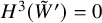 . Let
. Let

Then

However,
$\tilde {W} + \tilde {W}'$
 contains the entire two-dimensional weight space of
$\Lambda ^2\mathfrak {b} \otimes \Lambda ^2\mathfrak {b}$
contains the entire two-dimensional weight space of
$\Lambda ^2\mathfrak {b} \otimes \Lambda ^2\mathfrak {b}$
 of weight
$-3\rho $
of weight
$-3\rho $
 , and so
$\rho \not \in \operatorname {psupp}^3(Q)$
, and so
$\rho \not \in \operatorname {psupp}^3(Q)$
 . Thus
$s = 0$
. Thus
$s = 0$
 , as required.
Calculation 4.8. Suppose that
$l \ge 5$
 ,
$0 \le i \le 3$
,
$0 \le i \le 3$
 , and
$0 \le j \le 4$
, and
$0 \le j \le 4$
 . Then the cohomology group
$H^i(\Lambda ^j(\mathfrak {b} \oplus \mathfrak {b}))$
. Then the cohomology group
$H^i(\Lambda ^j(\mathfrak {b} \oplus \mathfrak {b}))$
 is as given in Table 2.
The group
$H^i(\Lambda ^j[\mathfrak {b} \oplus \mathfrak {b}])$
 . Cohomology groups which are zero are denoted by a dot, while those which are unknown are denoted by a question mark.
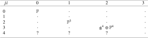
Table 2 Long description
The table is organized with index i as columns (0 to 3) and index j as rows (0 to 4).
* Row j equals 0: Column i equals 0 contains blackboard bold F. Columns 1, 2, and 3 contain dots.
* Row j equals 1: Columns 0, 1, 2, and 3 all contain dots.
* Row j equals 2: Column i equals 1 contains blackboard bold F super 3. Columns 0, 2, and 3 contain dots.
* Row j equals 3: Column i equals 2 contains fraktur g super 4 direct sum blackboard bold F super 4. Columns 0, 1, and 3 contain dots.
* Row j equals 4: Columns 0, 1, and 2 contain question marks. Column 3 contains a dot.
Proof. This is immediate from Calculations 4.3, 4.4 and 4.5 and the decompositions

and

which hold for
$l \ge 5$
 .
.
Remark 4.9. It appears that Calculation 4.5 is near the limit of what our ad hoc methods can handle. Using the programs of Hemelsoet and Voorhaar [Reference Hemelsoet and Voorhaar12], available at https://github.com/RikVoorhaar/bgg-cohomology, it is easy to verify all of the previous calculations over a field of characteristic zero. This implies that these calculations are correct in sufficiently large positive characteristic; however, it is not clear to us how to make this effective (their algorithm relies on the BGG resolution).
4.0.2 Twists
Calculation 4.10. Let
$\lambda \in X(T)_+$
 be a nonzero dominant weight. Suppose that
$l \ge 5$
be a nonzero dominant weight. Suppose that
$l \ge 5$
 . Then:
-
0. $H^i(\mathbb {F}(\lambda )) = 0$
for all
$i> 0$
; -
1. $H^i(\mathfrak {b}(\lambda )) = 0$
if
$i> 1$
, and
$H^1(\mathfrak {b}(\lambda )) = 0$
if
$\lambda - \rho $
is dominant or if
$l \ge 2 + \max (\left \langle \lambda , \alpha ^\vee \right \rangle , \left \langle \lambda , \beta ^\vee \right \rangle )$
; -
2. $H^i(\Lambda ^2[\mathfrak {b} \oplus \mathfrak {b}](\lambda )) = 0$
if
$i \ge 2$
; -
3. $H^3(\Lambda ^3[\mathfrak {b} \oplus \mathfrak {b}](\lambda )) = 0$
.










Proof. Recall that
$H^i(\mathbb {F}(\lambda )) = 0$
 for all
$i> 0$
for all
$i> 0$
 by Kempf’s vanishing theorem [Reference Jantzen14, Proposition II.4.5]. This deals immediately with part (0). Recall also from [Reference Jantzen14, Proposition II.5.4 (a)] that, if
$\mu \in X(T)$
by Kempf’s vanishing theorem [Reference Jantzen14, Proposition II.4.5]. This deals immediately with part (0). Recall also from [Reference Jantzen14, Proposition II.5.4 (a)] that, if
$\mu \in X(T)$
 with
$\left \langle \mu , \kappa ^\vee \right \rangle = -1$
with
$\left \langle \mu , \kappa ^\vee \right \rangle = -1$
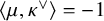 for some simple root
$\kappa $
for some simple root
$\kappa $
 , then
$H^i(\mathbb {F}(\mu )) = 0$
, then
$H^i(\mathbb {F}(\mu )) = 0$
 for all
$i \ge 0$
for all
$i \ge 0$
 . In particular, this implies that
$H^i(\mathbb {F}(\lambda )) = 0$
. In particular, this implies that
$H^i(\mathbb {F}(\lambda )) = 0$
 for all
$\lambda \in -\rho + X(T)_+$
for all
$\lambda \in -\rho + X(T)_+$
 and all
$i>0$
and all
$i>0$
 .
.
For part (1), if
$\lambda - \rho $
 is dominant, then every weight of
$\mathfrak {b}(\lambda )$
is dominant, then every weight of
$\mathfrak {b}(\lambda )$
 lies in
$-\rho + X(T)_+$
lies in
$-\rho + X(T)_+$
 and so
$H^i(\mathfrak {b}(\lambda )) = 0$
and so
$H^i(\mathfrak {b}(\lambda )) = 0$
 for all
$i> 0$
for all
$i> 0$
 . Otherwise, we have (without loss of generality) that
$\lambda = aL_1$
. Otherwise, we have (without loss of generality) that
$\lambda = aL_1$
 ; assume this now.
For every weight
$\mu $
 of
$\mathfrak {b}(\lambda )$
of
$\mathfrak {b}(\lambda )$
 , we have
$\mu \in -\rho + X(T)^+$
, we have
$\mu \in -\rho + X(T)^+$
 , or
$\mu = -\beta + aL_1$
, or
$\mu = -\beta + aL_1$
 and
$\left \langle \mu , \beta ^\vee \right \rangle = -2$
and
$\left \langle \mu , \beta ^\vee \right \rangle = -2$
 . We wish to show that
$H^i(\mathbb {F}(\mu ))$
. We wish to show that
$H^i(\mathbb {F}(\mu ))$
 vanishes in the latter case for
$i> 1$
vanishes in the latter case for
$i> 1$
 . By [Reference Jantzen14, Proposition II.5.4 (d)], we have

for all
$i> 1$
 Footnote 2. It follows that
$H^i(\mathfrak {b}(\lambda )) = 0$
Footnote 2. It follows that
$H^i(\mathfrak {b}(\lambda )) = 0$
 for all
$i\ge 2$
for all
$i\ge 2$
 .
.
Suppose now that
$l \ge 2 + a$
 . Then
$\mathfrak {b}(\lambda )$
. Then
$\mathfrak {b}(\lambda )$
 is BWB-good and
$\operatorname {psupp}^1(\mathfrak {b}(\lambda )) = \{\lambda \}$
is BWB-good and
$\operatorname {psupp}^1(\mathfrak {b}(\lambda )) = \{\lambda \}$
 . On the other hand, from the short exact sequence

we obtain a surjection
$H^0((\mathfrak {g}/\mathfrak {b})(\lambda )) \twoheadrightarrow H^1(\mathfrak {b}(\lambda ))$
 . But, using that
$\lambda = aL_1$
. But, using that
$\lambda = aL_1$
 ,
$\operatorname {psupp}^0((\mathfrak {g}/\mathfrak {b})(\lambda )) = \{\rho + \lambda , \beta + \lambda \}$
,
$\operatorname {psupp}^0((\mathfrak {g}/\mathfrak {b})(\lambda )) = \{\rho + \lambda , \beta + \lambda \}$
 which is disjoint from
$\{\lambda \}$
which is disjoint from
$\{\lambda \}$
 , and so

as required.
For part (2), as before, it is enough to consider weights
$\mu $
 of
$\Lambda ^2[\mathfrak {b} \oplus \mathfrak {b}](\lambda )$
of
$\Lambda ^2[\mathfrak {b} \oplus \mathfrak {b}](\lambda )$
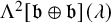 with
$\left \langle \mu + \rho , \alpha ^\vee \right \rangle < 0$
with
$\left \langle \mu + \rho , \alpha ^\vee \right \rangle < 0$
 . Any such weight
$\mu $
. Any such weight
$\mu $
 either lies in
$s_\alpha \cdot (-\rho + X(T)_+)$
either lies in
$s_\alpha \cdot (-\rho + X(T)_+)$
 , or is equal to
$-2\rho - L_3$
, or is equal to
$-2\rho - L_3$
 and so lies on the line
$\left \langle \mu , \beta ^\vee \right \rangle = -1$
and so lies on the line
$\left \langle \mu , \beta ^\vee \right \rangle = -1$
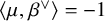 . In the latter case,
$H^i(\mathbb {F}(\mu )) = 0$
. In the latter case,
$H^i(\mathbb {F}(\mu )) = 0$
 for all i; in the former, as
$\left \langle \mu + \rho , \alpha ^\vee \right \rangle \ge -3$
for all i; in the former, as
$\left \langle \mu + \rho , \alpha ^\vee \right \rangle \ge -3$
 and
$l \ge 3$
and
$l \ge 3$
 , [Reference Jantzen14, Proposition II.5.4 (d)] implies that

for all
$i \ge 2$
 . Thus
$H^i(\Lambda ^2[\mathfrak {b} \oplus \mathfrak {b}](\lambda )) = 0$
. Thus
$H^i(\Lambda ^2[\mathfrak {b} \oplus \mathfrak {b}](\lambda )) = 0$
 for all
$i \ge 2$
for all
$i \ge 2$
 .
.
Finally, for part (3), suppose
$\mu $
 is a weight of
$\Lambda ^3[\mathfrak {b}\oplus \mathfrak {b}](\lambda )$
is a weight of
$\Lambda ^3[\mathfrak {b}\oplus \mathfrak {b}](\lambda )$
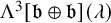 . By inspection of the weights of
$\Lambda ^3[\mathfrak {b} \oplus \mathfrak {b}]$
. By inspection of the weights of
$\Lambda ^3[\mathfrak {b} \oplus \mathfrak {b}]$
 and the assumption that
$l \ge 5$
and the assumption that
$l \ge 5$
 we see that either:
-
1. $\mu $
lies on one of the lines
$\left \langle \mu + \rho , \kappa \right \rangle = 0$
for some root
$\kappa $
; -
2. $\mu \in C^2_{\mathbb {Z}}$
; -
3. $\mu \in C^1_{\mathbb {Z}}$
and
$0 \le \left \langle \mu +\rho , \kappa \right \rangle \le 4$
for some simple root
$\kappa $
; or -
4. $\mu \in C^0_{\mathbb {Z}}$
.







In each case we have
$H^3(\mathbb {F}(\mu )) = 0$
 by [Reference Jantzen14]: Proposition II.5.4 (a) in case (1), Corollary II.5.5 (b) in case (2), Proposition II.5.4 (d) in case (3) and Theorem II.4.5 in case (4).
Calculation 4.11. Let
$\lambda \in X(T)_+$
 . If
$l \ge 5$
. If
$l \ge 5$
 then
then

whenever
$i> j$
 .
.
If
$l \ge 7$
 and
$i \ne 1$
and
$i \ne 1$
 , then

while

Proof. The statement in the case
$i> j$
 can be proved by applying [Reference Jantzen14, Proposition II.5.4] exactly as in Calculation 4.10, and we omit the details. We therefore focus on the case
$i = j$
can be proved by applying [Reference Jantzen14, Proposition II.5.4] exactly as in Calculation 4.10, and we omit the details. We therefore focus on the case
$i = j$
 ; by symmetry, it is enough to deal with
$\alpha $
; by symmetry, it is enough to deal with
$\alpha $
 . The reader may check that, in the calculations below, every representation to which we apply
$\operatorname {psupp}$
. The reader may check that, in the calculations below, every representation to which we apply
$\operatorname {psupp}$
 is BWB-good for
$l\ge 7$
is BWB-good for
$l\ge 7$
 .
.
If
$i = 0$
 then
$H^0(\mathbb {F}(\alpha )) = 0$
then
$H^0(\mathbb {F}(\alpha )) = 0$
 as
$\alpha $
as
$\alpha $
 is on the boundary of
$\overline {C}_{\mathbb {Z}}$
is on the boundary of
$\overline {C}_{\mathbb {Z}}$
 .
.
We have already shown that
$H^i(\mathfrak {b}(\alpha )) = 0$
 for
$i> 1$
for
$i> 1$
 . From the inclusion
$\mathfrak {b} \hookrightarrow \mathfrak {g}$
. From the inclusion
$\mathfrak {b} \hookrightarrow \mathfrak {g}$
 we obtain an inclusion

and so
$H^0(\mathfrak {b}(\alpha )) = 0$
 . Computing the Euler characteristic shows that
$H^1(\mathfrak {b}(\alpha )) \cong \mathfrak {g}$
. Computing the Euler characteristic shows that
$H^1(\mathfrak {b}(\alpha )) \cong \mathfrak {g}$
 .
.
We next show that
$H^1((\mathfrak {g}/\mathfrak {b})(\alpha )) = 0$
 . Indeed, this sits in a short exact sequence

and the outer terms are both zero.
Now, from the exact sequence

and the fact that
$H^2(\mathfrak {b}(\alpha )) = 0$
 , we obtain a surjection

As
$\operatorname {psupp}^2(\mathfrak {b}\otimes \mathfrak {b}(\alpha )) = \{0\}$
 we have that
$H^2(\mathfrak {b}\otimes \mathfrak {b}(\alpha )) \subset \mathbb {F}$
we have that
$H^2(\mathfrak {b}\otimes \mathfrak {b}(\alpha )) \subset \mathbb {F}$
 .
.
From the short exact sequence
$0 \to (\mathfrak {b} \otimes \mathfrak {g}/\mathfrak {b})(\alpha ) \to (\mathfrak {g} \otimes \mathfrak {g}/\mathfrak {b})(\alpha )\to (\mathfrak {g}/\mathfrak {b} \otimes \mathfrak {g}/\mathfrak {b})(\alpha ) \to 0$
 and the vanishing of
$H^1((\mathfrak {g}/\mathfrak {b})(\alpha ))$
and the vanishing of
$H^1((\mathfrak {g}/\mathfrak {b})(\alpha ))$
 we get a surjection

and hence a surjection

But
$\operatorname {psupp}^0(\mathfrak {g}/\mathfrak {b} \otimes \mathfrak {g}/\mathfrak {b}(\alpha ))$
 does not contain
$\{0\}$
does not contain
$\{0\}$
 , so we must have

from which we can obtain as in Calculation 4.8

Finally we do the case
$i = j = 3$
 . Here
$\operatorname {psupp}^3(\Lambda ^3\mathfrak {b}(\alpha )) = \emptyset $
. Here
$\operatorname {psupp}^3(\Lambda ^3\mathfrak {b}(\alpha )) = \emptyset $
 so it is enough to show that

From the usual exact sequence and the vanishing of
$H^3(\Lambda ^2\mathfrak {b}(\alpha ))$
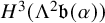 we obtain a surjection

But
$\operatorname {psupp}^2(\Lambda ^2\mathfrak {b} \otimes \mathfrak {g}/\mathfrak {b}(\alpha )) = \emptyset $
 and so

4.1 Results for the cohomology of sheaves on Z and Y
We now use the above results to calculate cohomology groups of particular coherent sheaves on Z and Y.
Lemma 4.12. Let
$\lambda \in X(T)_+$
 and suppose that
$l \ge 5$
and suppose that
$l \ge 5$
 . Then

for all
$i>0$
 .
.
Proof. Because the map
$\pi _Z:Z\rightarrow F$
 is affine, from Proposition 3.2 we have the following isomorphisms of cohomology groups:

So the question reduces to the calculation of the groups
$H^i(F,\operatorname {Sym}^n[\mathfrak {g}/\mathfrak {b}^2])$
 .
.
As in Section 4 of [Reference Vilonen and Xue23], one can consider the Koszul complex of
$0\to \mathfrak {b}^2 \to \mathfrak {g}^2\to \mathfrak {g}/\mathfrak {b}^2\to 0$
 and twist by
$\lambda $
and twist by
$\lambda $
 , giving us a resolution

We therefore have a spectral sequence

By Calculation 4.8 in the case of
$\lambda =0$
 , and Calculations 4.10 and 4.11 in the other cases, we see that
$H^{k+i}(\Lambda ^i[\mathfrak {b}^2](\lambda ))=0$
, and Calculations 4.10 and 4.11 in the other cases, we see that
$H^{k+i}(\Lambda ^i[\mathfrak {b}^2](\lambda ))=0$
 for any
$k>0$
for any
$k>0$
 and any
$i \ge 0$
and any
$i \ge 0$
 , and therefore
$H^k(\operatorname {Sym}[(\mathfrak {g}/\mathfrak {b})^2](\lambda ))=0$
, and therefore
$H^k(\operatorname {Sym}[(\mathfrak {g}/\mathfrak {b})^2](\lambda ))=0$
 for all
$k>0$
for all
$k>0$
 .
.
Remark 4.13. Lemma 4.12 appears as Corollary 4.3 in [Reference Ngo18] (and, for
$\lambda = 0$
 in characteristic 0, in [Reference Vilonen and Xue23], with a claim (Remark 6.2) that the result holds for
$l\ge 5$
in characteristic 0, in [Reference Vilonen and Xue23], with a claim (Remark 6.2) that the result holds for
$l\ge 5$
 ). We have given an alternative proof, as there appears to be a small issue in [Reference Ngo18] (and we also wish to obtain more refined information, such as about the
$H^0$
). We have given an alternative proof, as there appears to be a small issue in [Reference Ngo18] (and we also wish to obtain more refined information, such as about the
$H^0$
 ). The proof of Theorem 4.2 in [Reference Ngo18] requires the case
$s = 0$
). The proof of Theorem 4.2 in [Reference Ngo18] requires the case
$s = 0$
 (in the notation of that paper) as an inductive hypothesis, whereas it is deduced afterwards as a corollary. To repair that issue, we must show that
$H^i(\operatorname {Sym}^n(\mathfrak {n}^{*,r})(\lambda ))$
(in the notation of that paper) as an inductive hypothesis, whereas it is deduced afterwards as a corollary. To repair that issue, we must show that
$H^i(\operatorname {Sym}^n(\mathfrak {n}^{*,r})(\lambda ))$
 for all
$i \ge 1$
for all
$i \ge 1$
 and
$\lambda \in X(T)_+$
and
$\lambda \in X(T)_+$
 . Now, in the notation of that paper,
$\beta + \lambda \in \mathcal {A}_\alpha $
. Now, in the notation of that paper,
$\beta + \lambda \in \mathcal {A}_\alpha $
 . Then we have the exact sequence

and we can apply an appropriate inductive hypothesis to deduce the vanishing of the ith cohomology of the middle term from the vanishing of the ith cohomology of the outer terms.
Along with brevity, the advantage of this approach is that it applies without restriction on the characteristic, as it relies on the ‘Easy Lemma’ of [Reference Demazure6] and a vanishing result of [Reference Kumar, Lauritzen and Thomsen16] proved using Frobenius splitting.
Lemma 4.14. Suppose that
$l \ge 5$
 . Then we have

for all
$i> 0$
 and, for
$\lambda \in X(T)_+$
and, for
$\lambda \in X(T)_+$
 ,
,

for all
$i> 0$
 .
.
Proof. From Proposition 3.2 that
$\mathcal {I}_Y\cong \mathcal {O}_Z(\rho )$
 and
$\omega _Z\cong \mathcal {O}_Z(2\rho )$
and
$\omega _Z\cong \mathcal {O}_Z(2\rho )$
 . The lemma now follows from Lemma 4.12.
Corollary 4.15. Let
$l \ge 5$
 and
$\lambda \in X(T)_+$
and
$\lambda \in X(T)_+$
 . Then

for all
$i> 0$
 . Furthermore,
$H^i(Y, \omega _Y) = 0$
. Furthermore,
$H^i(Y, \omega _Y) = 0$
 for all
$i> 0$
for all
$i> 0$
 .
.
Proof. The first claim follows from Lemmas 4.12 and 4.14 and the long exact sequence in cohomology arising from

The second claim follows from the isomorphism
$\omega _Y \cong \mathcal {O}_Y(\rho )$
 proved in Proposition 3.2.
5 Equations for
$\mathcal {X}_{\operatorname {St}}$

In this section, we seek explicit equations for
$\mathcal {X}_{\operatorname {St}}$
 (or equivalently, for
$\mathcal {X}$
(or equivalently, for
$\mathcal {X}$
 ). For the generic fibre,
$\mathcal {X} \times _{\mathcal {O}} E$
). For the generic fibre,
$\mathcal {X} \times _{\mathcal {O}} E$
 , this was done by the first author.
Proposition 5.1. For
$n \ge 1$
 ,
$\mathcal {X}_E \subset GL_{n,E} \times GL_{n,E}$
,
$\mathcal {X}_E \subset GL_{n,E} \times GL_{n,E}$
 is the closed subscheme of pairs
$(\Sigma , \Phi )$
is the closed subscheme of pairs
$(\Sigma , \Phi )$
 such that

Proof. After a change of variables from the unipotent cone to the nilpotent cone via the logarithm map, this is a special case of Corollary 3.3 in [Reference Funck9]. (Note that in the nilpotent version, the equations making
$\log (\Sigma )$
 nilpotent are contained in the ideal generated by the coefficients of
$\Phi \log (\Sigma )\Phi ^{-1}-q\log (\Sigma )$
nilpotent are contained in the ideal generated by the coefficients of
$\Phi \log (\Sigma )\Phi ^{-1}-q\log (\Sigma )$
 – see Proposition 2.5 of [Reference Funck9]). The main idea is that, if
$\mathcal {C}\subseteq \mathrm {GL}_{n,E}$
– see Proposition 2.5 of [Reference Funck9]). The main idea is that, if
$\mathcal {C}\subseteq \mathrm {GL}_{n,E}$
 is the conjugacy class of
$\operatorname {diag}(1, q, \ldots , q^{n-1})$
is the conjugacy class of
$\operatorname {diag}(1, q, \ldots , q^{n-1})$
 , which is a smooth variety defined by the second equation above, then
$\mathcal {X}_E \to \mathcal {C}$
, which is a smooth variety defined by the second equation above, then
$\mathcal {X}_E \to \mathcal {C}$
 can be shown to be a vector bundle with fibre over
$\Phi \in \mathcal {C}$
can be shown to be a vector bundle with fibre over
$\Phi \in \mathcal {C}$
 given by

However, even for
$n = 2$
 , the subscheme of
$GL_{n, \mathcal {O}} \times GL_{n, \mathcal {O}}$
, the subscheme of
$GL_{n, \mathcal {O}} \times GL_{n, \mathcal {O}}$
 cut out by these equations is not
$\mathcal {O}$
cut out by these equations is not
$\mathcal {O}$
 -flat, and so does not coincide with
$\mathcal {X}$
-flat, and so does not coincide with
$\mathcal {X}$
 . To find the correct set of equations, we use the method of [Reference Snowden21]. We begin with a slight generalization of Proposition 2.1.5 of [Reference Snowden21].
Proposition 5.2. Let F be a scheme of finite type over
$\mathbb {F}$
 and
and

be a short exact sequence of vector bundles on F, with
$\epsilon = V \otimes _{\mathbb {F}} \mathcal {O}_F$
 for some
$\mathbb {F}$
for some
$\mathbb {F}$
 -vector space V. Let
$S=\operatorname {Sym}(V^{\ast })$
-vector space V. Let
$S=\operatorname {Sym}(V^{\ast })$
 , let Z be the total space of
$\nu ^{\ast }$
, let Z be the total space of
$\nu ^{\ast }$
 with
$\pi : Z \to F$
with
$\pi : Z \to F$
 the natural map, and let

There is a natural map of graded rings
$S \to R$
 .
.
Let
$\mathcal {L}$
 be a line bundle on F and let

a graded R-module. Suppose that
$H^i(F,\operatorname {Sym}(\nu )\otimes \mathcal {L})=0$
 whenever
$i>0$
whenever
$i>0$
 . Then

as graded vector spaces, where
$W[i]$
 is the vector space W living in degree i.
Proof. Recall from the proof of Proposition 2.1.5 of [Reference Snowden21] that we have a diagram

with the horizontal maps being the zero sections. Since
$Z \subset F \times V$
 is a closed subscheme, we may also regard quasicoherent
$\mathcal {O}_Z$
is a closed subscheme, we may also regard quasicoherent
$\mathcal {O}_Z$
 -modules as quasicoherent
$\mathcal {O}_{F \times V}$
-modules as quasicoherent
$\mathcal {O}_{F \times V}$
 -modules supported on Z. In particular, this applies to
$\pi ^{\ast }\mathcal {L}$
-modules supported on Z. In particular, this applies to
$\pi ^{\ast }\mathcal {L}$
 , and if
$q : F\times V \to F$
, and if
$q : F\times V \to F$
 is the projection, then
$\pi ^{\ast }\mathcal {L} = \mathcal {O}_Z \otimes q^{\ast }\mathcal {L}$
is the projection, then
$\pi ^{\ast }\mathcal {L} = \mathcal {O}_Z \otimes q^{\ast }\mathcal {L}$
 .
.
There are isomorphisms

The first isomorphism results from the hypothesis that

for all
$i>0$
 . The second is the base-change isomorphism of [22, Lemma 08IB].
As in the proof of Proposition 2.1.5 of [Reference Snowden21], the Koszul complex gives a quasi-isomorphism of complexes of coherent sheaves on
$F \times V$
 , graded as
$\mathcal {O}_V$
, graded as
$\mathcal {O}_V$
 -modules,

Here
$(-i)$
 is the shift operator on graded
$\mathcal {O}_V$
is the shift operator on graded
$\mathcal {O}_V$
 -modules. The differentials in the left-hand complex vanish on applying
$(i')^{\ast }$
-modules. The differentials in the left-hand complex vanish on applying
$(i')^{\ast }$
 , while the terms are flat
$\mathcal {O}_{F \times V}$
, while the terms are flat
$\mathcal {O}_{F \times V}$
 -modules, and so we get a quasi-isomorphism

in which the differentials in the left-hand complex are zero. Applying
$Rp^{\prime }_{\ast }$
 we therefore find that

as required.
We will always apply the lemma with
$V = (\mathfrak {g}^{\ast })^2 = \mathfrak {g}^2$
 and
$\xi = (\mathfrak {n}^\perp )^2 = \mathfrak {b}^2$
and
$\xi = (\mathfrak {n}^\perp )^2 = \mathfrak {b}^2$
 , so that
$\nu = (\mathfrak {g}/\mathfrak {b})^2 = (\mathfrak {n}^{\ast })^2$
, so that
$\nu = (\mathfrak {g}/\mathfrak {b})^2 = (\mathfrak {n}^{\ast })^2$
 and Z is the total space of the vector bundle
$\mathfrak {n}^2$
and Z is the total space of the vector bundle
$\mathfrak {n}^2$
 . Let
$R = H^0(Z, \mathcal {O}_Z)$
. Let
$R = H^0(Z, \mathcal {O}_Z)$
 . We have shown already that, if
$l> n$
. We have shown already that, if
$l> n$
 , then
$S \to R$
, then
$S \to R$
 is surjective, and so R is the coordinate ring of the image
$p(Z)$
is surjective, and so R is the coordinate ring of the image
$p(Z)$
 of Z in
$\mathfrak {g}^2$
of Z in
$\mathfrak {g}^2$
 (a variety over
$\mathbb {F}$
(a variety over
$\mathbb {F}$
 ). Let
$I = \ker (S \to R)$
). Let
$I = \ker (S \to R)$
 , which is also the ideal defining
$p(Z)$
, which is also the ideal defining
$p(Z)$
 . Our strategy will be to write down an ideal
$\tilde {I} \subset I$
. Our strategy will be to write down an ideal
$\tilde {I} \subset I$
 and deduce that
$\tilde {I} = I$
and deduce that
$\tilde {I} = I$
 by computing

using Proposition 5.2. In the case
$n = 3$
 , having determined
$p(Z)$
, having determined
$p(Z)$
 , we will then determine equations for
$X = p(Y)$
, we will then determine equations for
$X = p(Y)$
 .
.
Note that
$S = \operatorname {Sym}((\mathfrak {g}^{\ast })^2)$
 is the coordinate ring of the space of pairs of elements of
$\mathfrak {g} = \mathfrak {sl}_3$
is the coordinate ring of the space of pairs of elements of
$\mathfrak {g} = \mathfrak {sl}_3$
 , and we write
$(M, N)$
, and we write
$(M, N)$
 for the universal pair of matrices over S.
5.1 The case
$n=2$

In this case,
$Z = Y$
 is the variety whose
$\mathbb {F}$
is the variety whose
$\mathbb {F}$
 -points are pairs of commuting elements of
$\mathfrak {sl}_2$
-points are pairs of commuting elements of
$\mathfrak {sl}_2$
 . By Proposition 5.2 we obtain

Since
$\mathfrak {b} \cong \mathcal {O}(-1)^2$
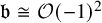 , we see that

is
$6$
 -dimensional.
Let
$\tilde {I}$
 be the ideal of S generated by the entries of
$MN - NM$
be the ideal of S generated by the entries of
$MN - NM$
 , by
$\operatorname {tr}(MN)$
, by
$\operatorname {tr}(MN)$
 , and by
$\det (M)$
, and by
$\det (M)$
 and
$\det (N)$
and
$\det (N)$
 . Then
$\tilde {I} \subset I$
. Then
$\tilde {I} \subset I$
 , and
$\tilde {I}/S_+\tilde {I}$
, and
$\tilde {I}/S_+\tilde {I}$
 is six-dimensional (as may easily be checked, noting that
$\operatorname {tr}(MN-NM) = 0$
is six-dimensional (as may easily be checked, noting that
$\operatorname {tr}(MN-NM) = 0$
 ), sitting in degree
$2$
), sitting in degree
$2$
 . It follows that
$\tilde {I} = I$
. It follows that
$\tilde {I} = I$
 and we have proved
Theorem 5.3. Let
$n = 2$
 . Then
$X \subset \mathfrak {g}^2$
. Then
$X \subset \mathfrak {g}^2$
 is the closed subscheme cut out by the equations
$\det (M) = \det (N) = 0$
is the closed subscheme cut out by the equations
$\det (M) = \det (N) = 0$
 , the entries of
$MN - NM$
, the entries of
$MN - NM$
 , and
$\operatorname {tr}(MN)$
, and
$\operatorname {tr}(MN)$
 .
.
We can apply this to
$\mathcal {X}$
 , recalling that we have shown that
$\mathcal {X} \otimes _{\mathcal {O}} \mathbb {F} = X$
, recalling that we have shown that
$\mathcal {X} \otimes _{\mathcal {O}} \mathbb {F} = X$
 .
.
Corollary 5.4. Let
$n = 2$
 . Then
$\mathcal {X} \subset GL_2 \times GL_2$
. Then
$\mathcal {X} \subset GL_2 \times GL_2$
 is the closed subscheme of pairs
$(\Sigma , \Phi )$
is the closed subscheme of pairs
$(\Sigma , \Phi )$
 such that

Moreover,
$\mathcal {X}_{\operatorname {St}}$
 is defined by the same equations but with the second equation replaced by
$q\operatorname {tr}(\Phi )^2 = 4\det (\Phi )$
is defined by the same equations but with the second equation replaced by
$q\operatorname {tr}(\Phi )^2 = 4\det (\Phi )$
 .
.
Proof. The statement for
$\mathcal {X}_{\operatorname {St}}$
 follows from that for
$\mathcal {X}$
follows from that for
$\mathcal {X}$
 and the discussion following Assumption 2.1.
To show that
$\mathcal {X}$
 is cut out by the given equations in
$GL_2 \times GL_2$
is cut out by the given equations in
$GL_2 \times GL_2$
 , we need only check this after
$\otimes _{\mathcal {O}} \mathbb {F}$
, we need only check this after
$\otimes _{\mathcal {O}} \mathbb {F}$
 and
$\otimes _{\mathcal {O}} E$
and
$\otimes _{\mathcal {O}} E$
 . After
$\otimes \mathbb {F}$
. After
$\otimes \mathbb {F}$
 , and writing
$\Phi = I + M$
, and writing
$\Phi = I + M$
 ,
$\Sigma = I + N$
,
$\Sigma = I + N$
 , we obtain exactly the equations generating the ideal
$\tilde {I}$
, we obtain exactly the equations generating the ideal
$\tilde {I}$
 above; thus we are done by Theorem 5.3.
By Proposition 5.1, the first three equations alone already define
$\mathcal {X}\otimes _{\mathcal {O}} E$
 , and this is a smooth variety. Since every point of
$\mathcal {X}(\overline {E})$
, and this is a smooth variety. Since every point of
$\mathcal {X}(\overline {E})$
 has
$\Phi \sim \operatorname {diag}(q,1)$
has
$\Phi \sim \operatorname {diag}(q,1)$
 , and the fourth equation is easily seen to hold at such points, we have that this equation is also contained in the defining ideal of
$\mathcal {X} \otimes _{\mathcal {O}} E$
, and the fourth equation is easily seen to hold at such points, we have that this equation is also contained in the defining ideal of
$\mathcal {X} \otimes _{\mathcal {O}} E$
 .
.
5.2 The case
$n = 3$

Recall that we have
$Y \subset Z$
 where Z is the total space of the vector bundle
$\mathfrak {n}^2$
where Z is the total space of the vector bundle
$\mathfrak {n}^2$
 on F and Y is the commuting subvariety, and we have
$X = \operatorname {Spec} \Gamma (Y, \mathcal {O}_Y)$
on F and Y is the commuting subvariety, and we have
$X = \operatorname {Spec} \Gamma (Y, \mathcal {O}_Y)$
 . If
$R = \Gamma (Z, \mathcal {O}_Z)$
. If
$R = \Gamma (Z, \mathcal {O}_Z)$
 then by the discussion above we have a surjective morphism
$S \to R$
then by the discussion above we have a surjective morphism
$S \to R$
 with kernel I.
Theorem 5.5. Suppose that
$n = 3$
 and that
$l \ge 5$
and that
$l \ge 5$
 . The homogeneous ideal
$I\trianglelefteq S$
. The homogeneous ideal
$I\trianglelefteq S$
 is generated by:
-
• $\operatorname {tr}(M^2), \operatorname {tr}(N^2), \operatorname {tr}(MN)$
(in degree 2); -
• $\operatorname {tr}(M^3), \operatorname {tr}(N^3)$
, and all the entries of $$\begin{align*}M^2N, N^2M, NM^2, MN^2\end{align*}$$(in degree 3).



Remark 5.6. In fact, the entries of
$MNM$
 and of
$NMN$
and of
$NMN$
 are also in the ideal generated by these equations, which may be easily checked by computer. One can take any two of
$M^2N, NM^2,$
are also in the ideal generated by these equations, which may be easily checked by computer. One can take any two of
$M^2N, NM^2,$
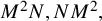 and
$MNM$
and
$MNM$
 in the generating set.
Proof. By Proposition 5.2, along with Calculation 4.8 and 4.5, we see that:

Hence we see that,

Let
$\tilde {I}$
 be the ideal of S generated by the elements listed in the statement of the theorem. Since all the elements of
$\tilde {I}$
be the ideal of S generated by the elements listed in the statement of the theorem. Since all the elements of
$\tilde {I}$
 vanish for
$M, N \in \mathfrak {n}$
vanish for
$M, N \in \mathfrak {n}$
 ,
$\tilde {I}\subset I$
,
$\tilde {I}\subset I$
 . We show that they are equal.
As
$\operatorname {tr}(M^2), \operatorname {tr}(MN)$
 , and
$\operatorname {tr}(N^2)$
, and
$\operatorname {tr}(N^2)$
 are all linearly independent, we see that they span the degree 2 subspace of
$\tilde {I}/S_+\tilde {I}$
are all linearly independent, we see that they span the degree 2 subspace of
$\tilde {I}/S_+\tilde {I}$
 . By a computer calculationFootnote 3 we see that the entries of
$M^2N$
. By a computer calculationFootnote 3 we see that the entries of
$M^2N$
 and
$NM^2$
and
$NM^2$
 span a 17-dimensional space modulo the subspace spanned by entries of
$\operatorname {tr}(M)^2N$
span a 17-dimensional space modulo the subspace spanned by entries of
$\operatorname {tr}(M)^2N$
 ,
$M\operatorname {tr}(MN)$
,
$M\operatorname {tr}(MN)$
 , and
$N \operatorname {tr}(M^2)$
, and
$N \operatorname {tr}(M^2)$
 so long as
$l> 2$
so long as
$l> 2$
 (this is just a matter of computing the invariant factors of an explicit finitely generated
$\mathbb {Z}$
(this is just a matter of computing the invariant factors of an explicit finitely generated
$\mathbb {Z}$
 -module). This same calculation also shows that the entries of
$MNM$
-module). This same calculation also shows that the entries of
$MNM$
 are in
$\tilde {I}$
are in
$\tilde {I}$
 . Therefore, using that there is a natural bigrading on S with respect to which
$\tilde {I}$
. Therefore, using that there is a natural bigrading on S with respect to which
$\tilde {I}$
 is bihomogeneous, we have

Thus
$\dim (\tilde {I}/S_+\tilde {I})_k = \dim (I/S_+I)_k$
 for all
$k \ge 0$
for all
$k \ge 0$
 , and so
$I = \tilde {I}$
, and so
$I = \tilde {I}$
 .
.
Theorem 5.7. Let J be the ideal of S determining the closed subscheme X. Then J is generated by
-
• $\operatorname {tr}(M),\operatorname {tr}(N)$
(in degree 1); -
• $\operatorname {tr}(M^2),\operatorname {tr}(MN), \operatorname {tr}(N^2)$
, and the entries of
$MN-NM$
(in degree 2); -
• $\operatorname {tr}(M^3),\operatorname {tr}(N^3)$
, and the entries of
$M^2N$
and
$MN^2$
(in degree 3).






Proof. Let
$i : Y \to Z$
 be the inclusion. Then we have that
$H^0(X, \mathcal {O}_X) = H^0(Z, i_{\ast }\mathcal {O}_Y)$
be the inclusion. Then we have that
$H^0(X, \mathcal {O}_X) = H^0(Z, i_{\ast }\mathcal {O}_Y)$
 and a short exact sequence

since, by Lemmas 2.3 and 4.12,
$H^1(Z, \mathcal {I}_Y)$
 vanishes.
We claim that
$I_X = H^0(Z, \mathcal {I}_Y)$
 is generated, as a (homogeneous) ideal of
$R = H^0(Z, \mathcal {O}_Z)$
is generated, as a (homogeneous) ideal of
$R = H^0(Z, \mathcal {O}_Z)$
 , by the entries of
$MN - NM$
, by the entries of
$MN - NM$
 . These entries give eight linearly independent elements of
$I_X$
. These entries give eight linearly independent elements of
$I_X$
 and it suffices to show that

By Lemma 2.3,
$\mathcal {I}_Y \cong \mathcal {O}_Z(\rho )$
 , locally (on F) generated in degree 2; hence
$I_X \cong H^0(Z, \mathcal {O}_Z(\rho ))(-2)$
, locally (on F) generated in degree 2; hence
$I_X \cong H^0(Z, \mathcal {O}_Z(\rho ))(-2)$
 as a graded S-module, where
$(-2)$
as a graded S-module, where
$(-2)$
 is the shift operator. By Proposition 5.2,

for
$i \ge 0$
 . The claim then follows from Calculation 4.10.
As J is the preimage of
$I_X$
 under
$S \to R$
under
$S \to R$
 , Theorem 5.7 then follows from Theorem 5.5.
We can also write down equations for
$\mathcal {X}$
 as follows:
Corollary 5.8. A complete set of equations defining the closed subscheme
$\mathcal {X}\subseteq \mathrm {GL}_3\times GL_3$
 over
$\mathcal {O}$
over
$\mathcal {O}$
 is as follows:

where
$\chi _A(x)$
 denotes the characteristic polynomial of A.
Similarly for
$\mathcal {X}_{\operatorname {St}}$
 , where the second equation is replaced by

and

Proof. The statement for
$\mathcal {X}_{\operatorname {St}}$
 follows from that for
$\mathcal {X}$
follows from that for
$\mathcal {X}$
 and the discussion following Assumption 2.1.
To show that
$\mathcal {X}$
 is cut out by the given equations in
$GL_3 \times GL_3$
is cut out by the given equations in
$GL_3 \times GL_3$
 , we need only check this after
$\otimes _{\mathcal {O}} \mathbb {F}$
, we need only check this after
$\otimes _{\mathcal {O}} \mathbb {F}$
 and
$\otimes _{\mathcal {O}} E$
and
$\otimes _{\mathcal {O}} E$
 . After
$\otimes \mathbb {F}$
. After
$\otimes \mathbb {F}$
 , and writing
$\Phi = I + M$
, and writing
$\Phi = I + M$
 ,
$\Sigma = I + N$
,
$\Sigma = I + N$
 , we obtain exactly the equations in Theorem 5.7, as required.
By Proposition 5.1, the first three equations alone already generate
$\mathcal {X}\otimes _{\mathcal {O}} E$
 , and this is a smooth variety. Since every point of
$\mathcal {X}(\overline {E})$
, and this is a smooth variety. Since every point of
$\mathcal {X}(\overline {E})$
 has
$\Phi \sim \operatorname {diag}(q^2,q,1)$
has
$\Phi \sim \operatorname {diag}(q^2,q,1)$
 , and the fourth, fifth, and sixth equations are easily seen to hold at such points, we have that these equations are also contained in the defining ideal of
$\mathcal {X} \otimes _{\mathcal {O}} E$
, and the fourth, fifth, and sixth equations are easily seen to hold at such points, we have that these equations are also contained in the defining ideal of
$\mathcal {X} \otimes _{\mathcal {O}} E$
 .
.
6 The Weil divisor class group
We compute the Weil divisor class group of X and the class of the canonical divisor. For
$n = 2$
 this gives another perspective on the calculations of [Reference Manning17]. One might hope for similar automorphic applications for
$n=3$
this gives another perspective on the calculations of [Reference Manning17]. One might hope for similar automorphic applications for
$n=3$
 , but there appear to be issues caused by the failure of the natural pairing on spaces of automorphic forms to be Hecke-equivariant (we thank Jeff Manning for explaining this point to us). Forthcoming work of Helm–Manning may resolve these issues.
6.1 Generalities on the class group
Let X be a Noetherian, integral, normal scheme. Recall from [22, Section 0AVT] that a coherent sheaf
$\mathcal {F}$
 on X is reflexive if the canonical map
$\mathcal {F} \to (\mathcal {F}^\vee )^\vee $
on X is reflexive if the canonical map
$\mathcal {F} \to (\mathcal {F}^\vee )^\vee $
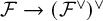 is an isomorphism, where
$\mathcal {F}^\vee = {\mathcal {H}\! \mathit {om}}_X(\mathcal {F},\mathcal {O}_X)$
is an isomorphism, where
$\mathcal {F}^\vee = {\mathcal {H}\! \mathit {om}}_X(\mathcal {F},\mathcal {O}_X)$
 . A reflexive sheaf on X of generic rank one is called divisorial. The set of isomorphism classes of divisorial sheaves on X forms a group that, by [22, Section 0EBK], is isomorphic to the Weil divisor class group
$\mathrm {Cl}(X)$
. A reflexive sheaf on X of generic rank one is called divisorial. The set of isomorphism classes of divisorial sheaves on X forms a group that, by [22, Section 0EBK], is isomorphic to the Weil divisor class group
$\mathrm {Cl}(X)$
 . If D is a Weil divisor on X then we write
$\mathcal {O}(D)$
. If D is a Weil divisor on X then we write
$\mathcal {O}(D)$
 for the associated divisorial sheaf.
If
$j : U \hookrightarrow X$
 is the inclusion of an open subscheme such that
$X \setminus U$
is the inclusion of an open subscheme such that
$X \setminus U$
 has codimension 2, then
$j^{\ast }$
has codimension 2, then
$j^{\ast }$
 and
$j_{\ast }$
and
$j_{\ast }$
 define quasi-inverse equivalences of categories between the set of reflexive sheaves on U and on X, so

If X is, in addition, Cohen–Macaulay, then the canonical sheaf
$\omega _X$
 is divisorial by [22, Lemma 0AY6, Lemma 0AWN] and we have
$\omega _X = j_{\ast }\omega _U$
is divisorial by [22, Lemma 0AY6, Lemma 0AWN] and we have
$\omega _X = j_{\ast }\omega _U$
 .
.
Lemma 6.1. Let
$f : E\rightarrow F$
 be a morphism of normal integral schemes of finite type over a field k, and suppose that f is faithfully flat with integral fibres. Let K be the function field of F and let
$C = E_K$
be a morphism of normal integral schemes of finite type over a field k, and suppose that f is faithfully flat with integral fibres. Let K be the function field of F and let
$C = E_K$
 be the generic fibre of f. Then there is an exact sequence

Proof. This is [Reference Fossum and Iversen8] Proposition 1.1, noting that a normal integral scheme of finite type over a field is Krull.
The maps
$\mathrm {Cl}(F) \to \mathrm {Cl}(E)$
 and
$\mathrm {Cl}(E) \to \mathrm {Cl}(C)$
and
$\mathrm {Cl}(E) \to \mathrm {Cl}(C)$
 are the functorial maps (see [Reference Fossum and Iversen8]). The map
$\delta $
are the functorial maps (see [Reference Fossum and Iversen8]). The map
$\delta $
 in the exact sequence is constructed as follows. Let
$u \in \Gamma (C, \mathcal {O}_C^\times )$
in the exact sequence is constructed as follows. Let
$u \in \Gamma (C, \mathcal {O}_C^\times )$
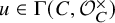 . Then u determines an element of the function field of E and hence a divisor
$\operatorname {\mathrm {Div}}(u)$
. Then u determines an element of the function field of E and hence a divisor
$\operatorname {\mathrm {Div}}(u)$
 on E, which one can show is the pullback of a divisor D on F. We define
$\delta (u) = \mathcal {O}(D) \in \mathrm {Cl}(X)$
on E, which one can show is the pullback of a divisor D on F. We define
$\delta (u) = \mathcal {O}(D) \in \mathrm {Cl}(X)$
 .
.
Lemma 6.2. Suppose that F is as in Lemma 6.1, that
$f : \mathcal {L} \to F$
 is a line bundle, and that E is the complement of the zero-section of f.
Choose an isomorphism
$\mathcal {L}_K \to \operatorname {Spec} K[t]$
 , so that t is a generator of

Then

where
$\delta $
 is the map from Lemma 6.1.
Proof. If
$D\subset F$
 is a closed integral subscheme of codimension 1 with generic point d, and if we choose a trivialization
$\mathcal {L}_d \cong \operatorname {Spec} \mathcal {O}_{F,d}[s]$
is a closed integral subscheme of codimension 1 with generic point d, and if we choose a trivialization
$\mathcal {L}_d \cong \operatorname {Spec} \mathcal {O}_{F,d}[s]$
 such that
$s = 0$
such that
$s = 0$
 is the zero section then we have

for some
$\kappa _D \in K$
 . We have that
$v_d(\kappa _D) = 0$
. We have that
$v_d(\kappa _D) = 0$
 for all but finitely many D and, by definition,

On the other hand, regard
$\mathcal {L}$
 as a sheaf on X that is locally free of rank 1, and let
$t^\vee \in \Gamma (\operatorname {Spec}(K), \mathcal {L}_K)$
as a sheaf on X that is locally free of rank 1, and let
$t^\vee \in \Gamma (\operatorname {Spec}(K), \mathcal {L}_K)$
 correspond to the section
$t^\vee : \operatorname {Spec}(K) \to \operatorname {Spec} K[t]$
correspond to the section
$t^\vee : \operatorname {Spec}(K) \to \operatorname {Spec} K[t]$
 such that
$(t^\vee )^{\ast }(t) = 1$
such that
$(t^\vee )^{\ast }(t) = 1$
 . Similarly, we have
$s^\vee \in \Gamma (X_{d}, \mathcal {L}_d)$
. Similarly, we have
$s^\vee \in \Gamma (X_{d}, \mathcal {L}_d)$
 , and the relation
$t^\vee = \kappa _D^{-1} s^\vee $
, and the relation
$t^\vee = \kappa _D^{-1} s^\vee $
 for each D as above. Then we have

from which the result follows.
6.2 Calculation of
$\mathrm {Cl}(X)$

Recall that we have the diagram

where Y is an irreducible variety, the map f is projective, and
$\pi $
 is a fibre bundle with fibres isomorphic to

by (the proof of) Lemma 2.3 part (2). Let
$U\subset X$
 be the open subscheme of points
$(M,N)\in X$
be the open subscheme of points
$(M,N)\in X$
 such that either M or N is regular nilpotent. If
$V = f^{-1}(U)$
such that either M or N is regular nilpotent. If
$V = f^{-1}(U)$
 then
$f|_V : V \to U$
then
$f|_V : V \to U$
 is an isomorphism, as in Lemma 3.1, while
$\pi |_V : V \to F$
is an isomorphism, as in Lemma 3.1, while
$\pi |_V : V \to F$
 is a fibre bundle with fibres

Lemma 6.3.
-
1. When $n = 2$
$$\begin{align*}C(\mathfrak{n})^{\mathrm{reg}}\cong\mathbb{A}^2\setminus\{(0,0)\},\end{align*}$$$Y \setminus V$
has codimension 2 in Y, and
$X \setminus U$
has codimension 3 in X.
-
2. When $n = 3$
$$\begin{align*}C(\mathfrak{n})^{\mathrm{reg}}\cong\mathbb{A}^2\setminus\{(0,0)\}\times \mathbb{G}_m\times \mathbb{A}^2,\end{align*}$$$Y \setminus V$
has codimension 1 in Y, and
$X \setminus U$
has codimension 2 in X.


Proof. If
$n = 2$
 , then
$C(\mathfrak {n}) = \mathfrak {n} \times \mathfrak {n} \cong \mathbb {A}^2$
, then
$C(\mathfrak {n}) = \mathfrak {n} \times \mathfrak {n} \cong \mathbb {A}^2$
 and
$C(\mathfrak {n})^{\mathrm {reg}} = \mathbb {A}^2 \setminus \{(0,0)\}$
and
$C(\mathfrak {n})^{\mathrm {reg}} = \mathbb {A}^2 \setminus \{(0,0)\}$
 . Therefore

Now

and X has dimension
$3$
 , so
$\mathrm {codim}(X\setminus U \subset X) = 3$
, so
$\mathrm {codim}(X\setminus U \subset X) = 3$
 . This proves part (1).
Now suppose that
$n = 3$
 . We write

which has dimension 5, and see that

Therefore

We have an isomorphism

with inverse defined by
$\frac {c}{a}\mapsto \lambda $
 when
$a\neq 0$
when
$a\neq 0$
 , and
$\frac {f}{d}\mapsto \lambda $
, and
$\frac {f}{d}\mapsto \lambda $
 when
$d\neq 0$
when
$d\neq 0$
 .
.
Finally, we compute the dimension of
$X \setminus U$
 . Since the locus
$M = N = 0$
. Since the locus
$M = N = 0$
 has codimension 8 in X, it is enough to compute the dimension of
$\{(M, N) \in X \setminus U : M \ne 0\}$
has codimension 8 in X, it is enough to compute the dimension of
$\{(M, N) \in X \setminus U : M \ne 0\}$
 . The projection map from this subset to
$\{M \in \mathfrak {g} : M^2 = 0, M \ne 0\}$
. The projection map from this subset to
$\{M \in \mathfrak {g} : M^2 = 0, M \ne 0\}$
 is a
$GL_3$
is a
$GL_3$
 -equivariant surjection. Its image is the orbit in
$\mathfrak {g}$
-equivariant surjection. Its image is the orbit in
$\mathfrak {g}$
 of the matrix
$M_0 = \begin {pmatrix} 0 & 0 & 1 \\ 0 & 0 & 0 \\ 0 & 0 & 0 \end {pmatrix}$
of the matrix
$M_0 = \begin {pmatrix} 0 & 0 & 1 \\ 0 & 0 & 0 \\ 0 & 0 & 0 \end {pmatrix}$
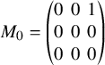 whose centralizer consists of all matrices of the form

and whose orbit in
$\mathfrak {g}$
 has dimension
$4$
has dimension
$4$
 (by the orbit-stabilizer theorem). The fibre in
$X\setminus U$
(by the orbit-stabilizer theorem). The fibre in
$X\setminus U$
 of
$M_0$
of
$M_0$
 is then

which has dimension
$2$
 , and so

as required.
Part (1) of the next theorem is [Reference Manning17] Proposition 3.14 part (1), proved there using toric geometry.
Theorem 6.4.
-
1. Suppose that $n = 2$
. There is an isomorphism $$\begin{align*}\nu : X^{\ast}(T) \to \mathrm{Cl}(X).\end{align*}$$Hence $\mathrm {Cl}(X) \cong \mathbb {Z}$
.
-
2. Suppose that $n = 3$
. There is a surjective homomorphism
$\nu : X^{\ast }(T) \to \mathrm {Cl}(X)$
with kernel generated by
$3(L_1 + L_3)$
. Therefore $$\begin{align*}\mathrm{Cl}(X)\cong X^{\ast}(T)/\left\langle 3(L_1 + L_3) \right\rangle \cong \mathbb{Z} \times \mathbb{Z}/3\mathbb{Z}.\end{align*}$$



Proof. The case
$n = 2$
 follows quickly from Lemma 6.3 part (1): we have

since
$X \setminus U$
 has codimension 2 in X,
$Y \setminus V$
has codimension 2 in X,
$Y \setminus V$
 has codimension 3 in Y, and Y is a vector bundle over F and so
$\mathrm {Cl}(Y) \cong \mathrm {Cl}(F)$
has codimension 3 in Y, and Y is a vector bundle over F and so
$\mathrm {Cl}(Y) \cong \mathrm {Cl}(F)$
 (e.g., by Lemma 6.1). As is well-known,

Suppose now that
$n = 3$
 . By Lemma 6.3 part (2), as the codimension of
$X\setminus U$
. By Lemma 6.3 part (2), as the codimension of
$X\setminus U$
 in X is 2, we have

Let K be the function field of F. By Lemma 6.1 and Lemma 6.3 part (2), we have an exact sequence

Since
$C(\mathfrak {n})^{\mathrm {reg}}_K$
 is an open subscheme of
$\mathbb {A}^5_K$
is an open subscheme of
$\mathbb {A}^5_K$
 ,
$\mathrm {Cl}(C(\mathfrak {n})^{\mathrm {reg}}_K) = 0$
,
$\mathrm {Cl}(C(\mathfrak {n})^{\mathrm {reg}}_K) = 0$
 . We have

It remains to compute the image of
$\delta $
 .
.
By Lemma 6.3, we have a morphism
$h : C(\mathfrak {n})_K \to \operatorname {Spec} K[\lambda , \lambda ^{-1}]$
 that induces an isomorphism

This morphism is B-equivariant if
$\lambda = \frac {c}{a} = \frac {f}{d}$
 is given weight
$L_1 - L_2 - (L_2 - L_3) = 3(L_1 + L_3)$
is given weight
$L_1 - L_2 - (L_2 - L_3) = 3(L_1 + L_3)$
 , and so we obtain a morphism

whose restriction to the generic fibres is h. We may therefore apply Lemma 6.2 and deduce that

The result follows.
Finally, we compute the canonical sheaf of X in terms of these isomorphisms. When
$n = 2$
 , this recovers [Reference Manning17] Proposition 3.14 part (2).
Corollary 6.5.
-
1. Suppose that $n = 2$
. Then
$\omega _X = \nu (2\rho )$
. -
2. Suppose that $n = 3$
. Then
$\omega _X=\nu (\rho )\in Cl(X)$
.

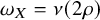


Proof. In either case, by Theorem 2.4, we have that
$\omega _X=f_{\ast }\omega _Y$
 .
.
If
$n = 2$
 then we have
$\omega _Y = \pi ^{\ast }\mathcal {O}(2\rho )$
then we have
$\omega _Y = \pi ^{\ast }\mathcal {O}(2\rho )$
 by Proposition 3.2. We therefore have

but also

as
$f : V \to U$
 is an isomorphism. Thus
$\omega _X= \nu (2\rho )$
is an isomorphism. Thus
$\omega _X= \nu (2\rho )$
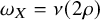 .
.
If
$n = 3$
 we again apply Proposition 3.2 to obtain

but also

as in the case
$n = 2$
 . Thus
$\omega _X = \nu (\rho )$
. Thus
$\omega _X = \nu (\rho )$
 .
.
6.3 Speculation on patched modules and their multiplicity
Let
$\iota : GL_3 \to GL_3$
 be the involution
$A \mapsto A^{-T}$
be the involution
$A \mapsto A^{-T}$
 , which induces involutions on X and on F that we also denote by
$\iota $
, which induces involutions on X and on F that we also denote by
$\iota $
 . On
$X^{\ast }(T)$
. On
$X^{\ast }(T)$
 this induces the involution interchanging
$L_1$
this induces the involution interchanging
$L_1$
 with
$-L_3$
with
$-L_3$
 .
.
Let D be a division algebra of degree
$3$
 over a local field F with residue field of order q. One expects (as in [Reference Zhu24, Conjecture 4.5.1]) a functor from the category of finitely generated smooth
$\mathbb {F}$
over a local field F with residue field of order q. One expects (as in [Reference Zhu24, Conjecture 4.5.1]) a functor from the category of finitely generated smooth
$\mathbb {F}$
 -representations of
$D^\times $
-representations of
$D^\times $
 to the derived category of coherent sheaves on X. In a global context, the completion of this functor at the origin of X should be realized by a ‘patching functor’ constructed using an appropriate unitary group. Applying this functor to
$\operatorname {ind}_{F^\times \mathcal {O}_D^\times }^{D^\times }(\mathbb {F})$
to the derived category of coherent sheaves on X. In a global context, the completion of this functor at the origin of X should be realized by a ‘patching functor’ constructed using an appropriate unitary group. Applying this functor to
$\operatorname {ind}_{F^\times \mathcal {O}_D^\times }^{D^\times }(\mathbb {F})$
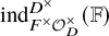 we expect to obtain a coherent sheaf
$\mathcal {M}$
we expect to obtain a coherent sheaf
$\mathcal {M}$
 on
$X^\wedge _0$
on
$X^\wedge _0$
 with the following properties:
-
1. $\mathcal {M}$
is maximal Cohen–Macaulay on
$X^\wedge _0$
of generic rank one (and hence divisorial); -
2. $\iota $
-self-duality:
${\mathcal {H}\! \mathit {om}}_{X^\wedge _0}(\mathcal {M}, \omega _{X^\wedge _0}) \cong \iota ^{\ast }\mathcal {M}$
.



In [Reference Manning17], it was shown (in the patching context) that these properties characterize
$\mathcal {M}$
 in the case
$n = 2$
in the case
$n = 2$
 , and this was used to prove a new global multiplicity 2 result for mod l automorphic forms. For that it is necessary to pass to the completion of X, which is subtle in the context of the class group. As there are other, more serious, issues arising from the natural pairing on the patched module not being Hecke-equivariant, we don’t pursue this and simply ask (for
$n = 3$
, and this was used to prove a new global multiplicity 2 result for mod l automorphic forms. For that it is necessary to pass to the completion of X, which is subtle in the context of the class group. As there are other, more serious, issues arising from the natural pairing on the patched module not being Hecke-equivariant, we don’t pursue this and simply ask (for
$n = 3$
 ) to what extent the above properties characterize
$\mathcal {M}$
) to what extent the above properties characterize
$\mathcal {M}$
 on X.
on X.
The forthcoming work of Helm and Manning, already alluded to, should add a third property to the above list allowing one to identify
$\mathcal {M} \hat {\otimes }_{\mathcal {O}^\wedge _{X_0}} \mathcal {M}$
 as an element of the class group. As we have shown that the class group is
$2$
as an element of the class group. As we have shown that the class group is
$2$
 -torsion free, we expect that this will make it possible to identify
$\mathcal {M}$
-torsion free, we expect that this will make it possible to identify
$\mathcal {M}$
 .
.
Proposition 6.6. Suppose that
$n = 3$
 and that
$\mathcal {M}$
and that
$\mathcal {M}$
 is a divisorial sheaf on X with
$\mathcal {M} = \nu (w)$
is a divisorial sheaf on X with
$\mathcal {M} = \nu (w)$
 for
$w\in X(T)$
for
$w\in X(T)$
 . Then
${\mathcal {H}\! \mathit {om}}_X(\mathcal {M}, \omega _X) \cong \iota ^{\ast }\mathcal {M}$
. Then
${\mathcal {H}\! \mathit {om}}_X(\mathcal {M}, \omega _X) \cong \iota ^{\ast }\mathcal {M}$
 if and only if

Proof. The map
$\nu $
 is easily seen to be
$\iota $
is easily seen to be
$\iota $
 -equivariant. If
$\mathcal {M} = \nu (aL_1 - bL_3)$
-equivariant. If
$\mathcal {M} = \nu (aL_1 - bL_3)$
 we have

and

These are equal if and only if

for some
$k \in \mathbb {Z}$
 . This holds if and only if
$a + b = 1$
. This holds if and only if
$a + b = 1$
 and
$k = 0$
and
$k = 0$
 . The different possibilities for
$b \bmod 3$
. The different possibilities for
$b \bmod 3$
 give the result.
We can explicitly describe
$\nu (w)$
 in these cases.
Lemma 6.7. Suppose that
$w \in X^{\ast }(T)$
 is such that
$Rf_{\ast }\mathcal {O}(w)$
is such that
$Rf_{\ast }\mathcal {O}(w)$
 and
$Rf_{\ast }(\rho - w)$
and
$Rf_{\ast }(\rho - w)$
 are each concentrated in degree zero. Then
$f_{\ast }\mathcal {O}(w)$
are each concentrated in degree zero. Then
$f_{\ast }\mathcal {O}(w)$
 is Cohen–Macaulay and

Proof. That
$f_{\ast }\mathcal {O}(w)$
 is Cohen–Macaulay is [Reference Hacon and Witaszek10] Proposition 2.2. It is therefore reflexive. The final claim follows as, if
$j : U \hookrightarrow X$
is Cohen–Macaulay is [Reference Hacon and Witaszek10] Proposition 2.2. It is therefore reflexive. The final claim follows as, if
$j : U \hookrightarrow X$
 is the natural inclusion, then
$X \setminus U$
is the natural inclusion, then
$X \setminus U$
 has codimension 2 and
$j^{\ast }f_{\ast }\mathcal {O}(w) = j^{\ast }\nu (w)$
has codimension 2 and
$j^{\ast }f_{\ast }\mathcal {O}(w) = j^{\ast }\nu (w)$
 by construction.
Proposition 6.8. Let
$l \ge 5$
 and
$\lambda = L_1, -L_3$
and
$\lambda = L_1, -L_3$
 , or
$2L_1 + L_3$
, or
$2L_1 + L_3$
 (as in Proposition 6.6). Then

is Cohen–Macaulay.
Proof. By Proposition 4.15,
$H^i(Y, \mathcal {O}_Y(\lambda ))$
 and
$H^i(Y, \mathcal {O}_Y(\rho - \lambda ))$
and
$H^i(Y, \mathcal {O}_Y(\rho - \lambda ))$
 vanish for each of these values of
$\lambda $
vanish for each of these values of
$\lambda $
 and for all
$i> 0$
and for all
$i> 0$
 . Since X is affine, we obtain exactly the vanishing of
$R^if_{\ast }$
. Since X is affine, we obtain exactly the vanishing of
$R^if_{\ast }$
 required to apply Lemma 6.7 to these
$\lambda $
required to apply Lemma 6.7 to these
$\lambda $
 , and the Proposition follows.
Let
$x \in X$
 be the point
$(0,0)$
be the point
$(0,0)$
 . If
$\mathcal {M}$
. If
$\mathcal {M}$
 is a coherent
$\mathcal {O}_X$
is a coherent
$\mathcal {O}_X$
 -module, then we call
$\dim _{\mathbb {F}}(\mathcal {M}\otimes _{\mathcal {O}_x}\mathbb {F})$
-module, then we call
$\dim _{\mathbb {F}}(\mathcal {M}\otimes _{\mathcal {O}_x}\mathbb {F})$
 the multiplicity of
$\mathcal {M}$
the multiplicity of
$\mathcal {M}$
 (at the origin). When
$\mathcal {M}^\wedge _x$
(at the origin). When
$\mathcal {M}^\wedge _x$
 arises as a patched module, this multiplicity will be the multiplicity of a system of Hecke eigenvalues in a certain space of mod l automorphic forms, as in [Reference Manning17] (see also [Reference Calegari and Geraghty3, Section 4.1] when
$l =p$
arises as a patched module, this multiplicity will be the multiplicity of a system of Hecke eigenvalues in a certain space of mod l automorphic forms, as in [Reference Manning17] (see also [Reference Calegari and Geraghty3, Section 4.1] when
$l =p$
 ). When
$\mathcal {M} = \omega _X$
). When
$\mathcal {M} = \omega _X$
 , this number is known as the type of the Cohen–Macaulay local ring
$\mathcal {O}_{X,x}$
, this number is known as the type of the Cohen–Macaulay local ring
$\mathcal {O}_{X,x}$
 .
.
Proposition 6.9. Let
$\lambda \in \{L_1, -L_3, 2L_1 + L_3, L_1 - L_3\}$
 and let
$l\ge 5$
and let
$l\ge 5$
 with
$l \ge 7$
with
$l \ge 7$
 if
$\lambda = 2L_1 + L_3$
if
$\lambda = 2L_1 + L_3$
 . Let
$m(\lambda )$
. Let
$m(\lambda )$
 be the multiplicity of
$\nu (\lambda ) = f_{\ast }\mathcal {O}_Y(\lambda )$
be the multiplicity of
$\nu (\lambda ) = f_{\ast }\mathcal {O}_Y(\lambda )$
 . Then
$m(\lambda )$
. Then
$m(\lambda )$
 is as in Table 3.
Multiplicities of
$\nu (\lambda )$
 .
.
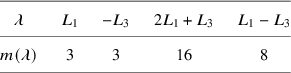
Table 3 Long description
The table consists of two rows and five columns.
Header Row:
- Column 1: lambda
- Column 2: L sub 1
- Column 3: negative L sub 3
- Column 4: 2 L sub 1 plus L sub 3
- Column 5: L sub 1 minus L sub 3
Data Row (m open parenthesis lambda close parenthesis):
- Column 1: m open parenthesis lambda close parenthesis
- Column 2: 3
- Column 3: 3
- Column 4: 16
- Column 5: 8
Proof. Let
$\lambda $
 be one of the weights occurring in the proposition and let
$M = H^0(Z, \mathcal {O}_Z(\lambda ))$
be one of the weights occurring in the proposition and let
$M = H^0(Z, \mathcal {O}_Z(\lambda ))$
 and
$N = H^0(Y, \mathcal {O}_Y(\lambda ))$
and
$N = H^0(Y, \mathcal {O}_Y(\lambda ))$
 . As in Section 5, by Lemma 4.12 we are in the situation of Proposition 5.2 with F the flag variety of
$\mathrm {GL}_3$
. As in Section 5, by Lemma 4.12 we are in the situation of Proposition 5.2 with F the flag variety of
$\mathrm {GL}_3$
 , the short exact sequence

being

and
$\mathcal {L} = \mathcal {O}_F(\lambda )$
 . We define
$S=\operatorname {Sym}[(\mathfrak {g}^{*})^2]$
. We define
$S=\operatorname {Sym}[(\mathfrak {g}^{*})^2]$
 as in Proposition 5.2, and define

Thus (and recalling that, as in the proof of Theorem 5.7,
$H^1(Z, \mathcal {I}_Y)$
 vanishes) we have morphisms of graded algebras

which fit into the following diagram:

Here, the schemes on the right are all affine, the schemes in the middle are all fibre bundles over F, and the vertical arrows are closed immersions.
Let
$M = H^0(Z, \mathcal {O}(\lambda ))$
 , a graded S-module. Then Proposition 5.2 applies and we have

by Calculations 4.10 and 4.11. In either case we see that
$\dim (M\otimes _S\mathbb {F})$
 is as given in Table 3.
By Proposition 4.15 we have

for
$i> 0$
 . We therefore have a short exact sequence of graded S-modules

Since
$\pi _{\ast }\mathcal {I}_Y(\lambda )$
 is (locally on F) generated in degree 2,
$H^0(Z, \mathcal {I}_Y(\lambda ))$
is (locally on F) generated in degree 2,
$H^0(Z, \mathcal {I}_Y(\lambda ))$
 is generated in degrees
$\ge 2$
is generated in degrees
$\ge 2$
 . We have shown that M is generated in degrees
$\le 1$
. We have shown that M is generated in degrees
$\le 1$
 , and therefore

is an isomorphism. As

we obtain the result.
Acknowledgements
We thank Jeffrey Manning for helpful correspondence about this research.
Much of this work was carried out during the first author’s PhD, funded by the Engineering and Physical Sciences Research Council.




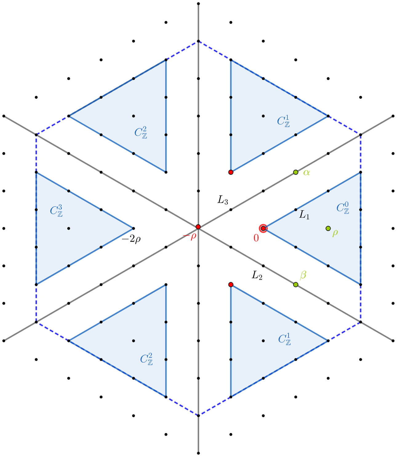

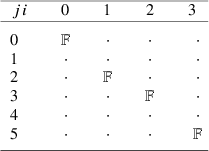

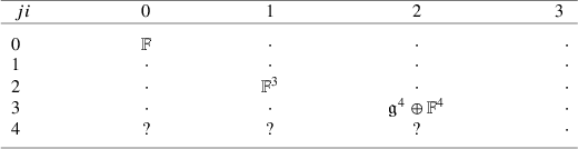

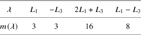


 Open access

