Ecological Gradients

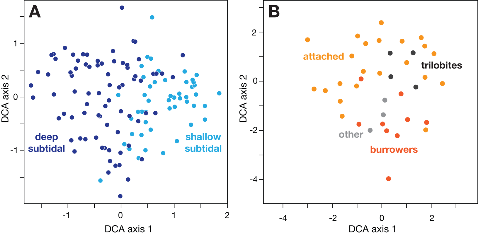
Although numerous factors control the ecological distribution of species, the application of gradient analysis (Whittaker Reference Whittaker1967) considerably simplifies the coordinated effects of these factors. Ordination methods such as nonmetric multidimensional scaling (NMS) and detrended correspondence analysis (DCA; Kruskal Reference Kruskal1964; Hill and Gauch Reference Hill and Gauch1980; Jongman et al. Reference Jongman, Ter Braak and Van Tongeren1995; Legendre and Legendre Reference Legendre and Legendre1998; Borcard et al. Reference Borcard, Gillet and Legendre2018) also provide a means for identifying the principal sources of variation in the ecological composition of communities (Fig. 1). For example, in shallow-marine (<200 m) settings, numerous physical and chemical parameters that affect the distribution of species vary with water depth, such as grain size, bed shear stress, oxygen, sunlight, salinity, temperature, and nutrients. As a result, water depth is the primary ecological gradient in marine benthic communities and is a proxy for a complex chemical and physical gradient that also includes species interactions (see reviews in Patzkowsky and Holland Reference Patzkowsky and Holland2012; Holland Reference Holland2023). In terrestrial settings, the variation in temperature, precipitation, and soil moisture with elevation cause it to be the principal ecological gradient (Holland and Loughney Reference Holland and Loughney2021). These gradients are ubiquitous in modern and ancient marine and nonmarine systems.

Figure 1. Coding ordination scores of samples and taxa can reveal the origin of the axes, shown with an example from the C2 sequence of the Upper Ordovician of the Cincinnati Arch, USA (data from Holland and Patzkowsky Reference Holland and Patzkowsky2007). A, Sample scores coded by lithofacies reveal that detrended correspondence analysis (DCA) axis 1 is correlated with water depth. B, Taxon scores coded by life habit demonstrate that DCA axis 2 is correlated with substrate characteristics, with burrowers associated with soft muds at low axis 2 scores and attached species associated with shelly gravels at high axis 2 scores.

Species distributions along these ecological gradients can be described with species response curves, which describe species’ abundance or probability of occurrence as a function of the position along an ecological gradient (e.g., water depth, elevation; Gauch and Whittaker Reference Gauch and Whittaker1976; Austin Reference Austin1987; Jongman et al. Reference Jongman, Ter Braak and Van Tongeren1995). Most commonly, the shape of these response curves is Gaussian or a skewed Gaussian; bimodal, multimodal, irregular, and flat response curves are far less common (Minchin Reference Minchin1989). The importance of these response curves is that the abundance and probability of occurrence will hit a peak (called peak abundance) at a particular position along a gradient (the preferred environment), and they will decrease away from this position depending on the environmental tolerance of a species. In shallow-marine systems, these response curves are sometimes surprisingly tight. For example, changes in water depth of even a few meters are accompanied by substantial changes in species abundance (Horton et al. Reference Horton, Edwards, Lloyd, Shennan and Andrews2000; Scarponi and Kowalewski Reference Scarponi and Kowalewski2004; Brown and Larina Reference Brown and Larina2019). Species in deeper-water systems would be expected to have broader tolerances, although species tolerances in offshore settings can sometimes be remarkably narrow (e.g., Holland et al. Reference Holland, Miller, Meyer and Dattilo2001).

Stratigraphic Architecture

That water depth and elevation are the principal ecological gradients takes on special significance, because water depth and elevation change systematically in the stratigraphic record through changes in the rates of accommodation and sedimentation. Accommodation, the space in which sediment can accumulate, is generated by tectonic subsidence, plus eustasy in marine systems and lake level in lacustrine systems. The combination of these drivers is what creates sequence-stratigraphic architecture (Van Wagoner et al. Reference Van Wagoner, Mitchum, Campion and Rahmanian1990; Catuneanu Reference Catuneanu2006; Catuneanu et al. Reference Catuneanu, Abreu, Bhattacharya, Blum, Dalrymple, Eriksson and Fielding2009; Neal and Abreu Reference Neal and Abreu2009), specifically the formation of subaerial unconformities and other hiatal surfaces, the lateral distribution of sedimentary facies, transgressions and regressions, and variations in sedimentation rates. In marine and coastal systems, these drivers produce systems tracts characterized by their positions, internal stacking patterns of strata, and shoreline trajectories. In nonmarine systems, systems tracts are characterized by position, channel stacking patterns, types of paleosols, and various other facies characteristics (Catuneanu Reference Catuneanu2006; Holland and Loughney Reference Holland and Loughney2021).

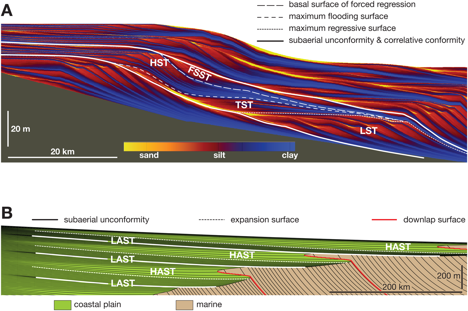
Although there are several approaches to defining these systems tracts (Catuneanu et al. Reference Catuneanu, Abreu, Bhattacharya, Blum, Dalrymple, Eriksson and Fielding2009), the most common model includes a lowstand systems tract (LST), transgressive systems tract (TST), highstand systems tract (HST), and falling-stage systems tract (FSST; Fig. 2A). In nonmarine systems, a low-aggradation systems tract (LAST) and high-aggradation systems tract (HAST) are the most widely used (Martinsen et al. Reference Martinsen, Ryseth, Helland-Hansen, Flesche, Torkildsen and Idil1999; Catuneanu Reference Catuneanu2006; Holland and Loughney Reference Holland and Loughney2021; Loughney and Holland Reference Loughney and Holland2023; Rogers et al. Reference Rogers, Eberth and Ramezani2023; Fig. 2B). Systems tracts record distinct patterns of change in water depth and elevation, including progressive trends as well as surfaces of abrupt change. For example, the HST displays increasingly rapid upward shallowing punctuated by relatively minor surfaces of abrupt deepening (flooding surfaces); the LST is similar, but the upward trend slows rather than accelerates. The TST displays net upward deepening, composed in detail of major flooding surfaces of abrupt deepening that separate intervals of minor shallowing. The FSST displays net upward shallowing punctuated by surfaces of abrupt shallowing (surfaces of forced regression).

Figure 2. Stratigraphic cross sections showing systems tracts and surfaces in marine and nonmarine settings. A, Cross section is model output from the basin simulation model sedflux (Hutton and Syvitski Reference Hutton and Syvitski2008). FSST, falling-stage systems tract; HST, highstand systems tract; LST, lowstand systems tract; TST, transgressive systems tract. B, Cross section is model output from the basin simulation model strataR (Holland Reference Holland2022a). Black lines are evenly spaced timelines, which can be used to infer aggradation rates. HAST, high-accommodation systems tract; LAST, low-accommodation systems tract.

Stratigraphic architecture varies markedly depending on the spatial pattern and temporal changes in subsidence rate, the rates and timescales of eustatic sea-level change, and the nature of how sediment is produced and transported, itself reflecting climate, topography, source area, and biogenic production (Catuneanu Reference Catuneanu2006). Understanding these controls has been a primary and ongoing focus of research in sedimentary geology for decades. For example, stratigraphic architecture can differ on opposite sides of a sedimentary basin depending on subsidence rates and the relative contributions of siliciclastic and carbonate sediment (Tomašových et al. 2022).

This is significant for the fossil record, because the stratigraphic record in which it is housed is highly structured and nonuniform, although the structure varies for all the reasons mentioned earlier. Sedimentation rates vary widely and predictably. Water depth and elevation change continuously, progressively in some cases, and abruptly in others. Subaerial unconformities occur in predictable places laterally and vertically. As a result, time is not preserved uniformly in strata, and preserved habitats are always in flux. Moreover, the stratigraphic record varies markedly and predictably along depositional dip (Fig. 3). This view of stratigraphy radically changes how we approach the fossil record, because constancy in sedimentation rates and ecological settings can rarely be assumed. The probability of preservation of fossil species is therefore rarely uniform but is instead in constant flux. Any interpretation of the fossil record must be based on this reality. Moreover, these changes are not random but are instead highly structured.

Figure 3. Depositional strike and dip, illustrated with the coast of Egypt at the Nile Delta. Map from Google Earth Pro. Depositionally updip areas are toward the sediment source (typically landward), and depositionally downdip areas are distal to the sediment source and therefore more commonly sediment starved.

Tests of Key Concepts in the Po Plain of Italy

Paleobiology gets increasingly more challenging into deep time for two reasons. The first is decreasing geochronological precision in older rocks. For example, typical uncertainties in Pleistocene strata using ¹⁴C and ²³⁰Th are less than ±2 kyr, and lower than ±200 yr for dates younger than 15 ka (e.g., Leigh Reference Leigh, Greenberg and Collins2016; Railsback et al. Reference Railsback, Brook, Liang, Voarintsoa, Cheng and Edwards2018). In contrast, U–Pb age uncertainties in the Late Ordovician range from ±170 kyr to ±340 kyr (Ling et al. Reference Ling, Zhan, Wang, Wang, Amelin, Tang and Liu2019), up to 20 times the duration of the Holocene. The second issue is that the ecology of species is increasingly poorly known into deep time. In the younger parts of the fossil record, fossil species may still be extant, and their ecology today is commonly a reasonable proxy for their ecology in the fossil record. In deeper time, proxies for extinct species are at higher taxonomic levels, and niche evolution (see Blois et al. 2024) makes inferences even more tenuous.

An extraordinary series of studies in late Pleistocene to Holocene deposits of the Po River delta in northern Italy avoids both complications through its geologically young age (Scarponi and Kowalewski Reference Scarponi and Kowalewski2004, Reference Scarponi and Kowalewski2007; Scarponi et al. Reference Scarponi, Kaufman, Amorosi and Kowalewski2013, Reference Scarponi, Azzarone, Kusnerik, Amorosi, Bohacs, Drexler and Kowalewski2017; Wittmer et al. Reference Wittmer, Dexter, Scarponi, Amorosi and Kowalewski2014; Huntley and Scarponi Reference Huntley and Scarponi2015; Kowalewski et al. Reference Kowalewski, Wittmer, Dexter, Amorosi and Scarponi2015; Nawrot et al. Reference Nawrot, Scarponi, Azzarone, Dexter, Kusnerik, Wittmer, Amorosi and Kowalewski2018). These studies provide critical tests of many aspects of stratigraphic paleobiology.

The studies are built on a well-delineated sequence-stratigraphic framework assembled from cores arrayed across depositional dip and depositional strike (Amorosi et al. Reference Amorosi, Centineo, Colalongo, Paasini, Sarti and Vaiani2003, Reference Amorosi, Colalongo, Fiorini, Fusco, Pasini, Vaiani and Sarti2004). Within these cores, mollusks were counted at multiple horizons (Scarponi and Kowalewski Reference Scarponi and Kowalewski2004). Ultimately, the dataset included 16 cores and 131,780 specimens in 234 species (Wittmer et al. Reference Wittmer, Dexter, Scarponi, Amorosi and Kowalewski2014; Kowalewski et al. Reference Kowalewski, Wittmer, Dexter, Amorosi and Scarponi2015), although the original dataset was less than a fifth of that. Counts of foraminifera, ostracods, and pollen were also analyzed in some studies (Amorosi et al. Reference Amorosi, Colalongo, Fiorini, Fusco, Pasini, Vaiani and Sarti2004, Reference Amorosi, Rossi, Scarponi, Vaiani and Ghosh2014). ¹⁴C-age dates were obtained throughout, supplemented by dated pollen correlations to other European sites. Selected shells were dated individually with amino acid racemization and calibrated with ¹⁴C (Scarponi et al. Reference Scarponi, Kaufman, Amorosi and Kowalewski2013) with precisions of ±100–300 yr. Because most of these species are extant in the Mediterranean, their modern ecological distributions relative to substrate and water depth are well understood (Pérès and Picard Reference Pérès and Picard1964; Pérès Reference Pérès1967; Dominici and Scarponi Reference Dominici and Scarponi2020) and accessible through a database operated by the New Technologies, Energy, and Environmental Agency (ENEA; Wittmer et al. Reference Wittmer, Dexter, Scarponi, Amorosi and Kowalewski2014).

One of the original goals of these studies was to test interpretations made from ordinations of fossil assemblages, specifically that axis 1 of some ordination methods is commonly correlated with water depth (e.g., Holland et al. Reference Holland, Miller, Meyer and Dattilo2001; Miller et al. Reference Miller, Holland, Meyer and Dattilo2001). The most common of these methods are DCA and NMS. The significance of axis 1 is that it reflects the greatest source of variation in the composition of fossil assemblages.

Salient Results

The Po Plain studies reach several significant conclusions, and they are encouraging news for stratigraphic paleobiology in deep time. First, indirect ordination techniques like DCA perform just as well as direct ordination techniques in their ability to recover ecological gradients (Wittmer et al. Reference Wittmer, Dexter, Scarponi, Amorosi and Kowalewski2014). This is important in deep time, where independent estimates of water-depth preferences of taxa are unavailable, rendering direct ordination impossible. This also confirms interpretations of ancient fossil assemblages, where a water-depth gradient is inferred based on lithofacies (e.g., Cisne and Rabe Reference Cisne and Rabe1978) or sequence-stratigraphic architecture (e.g., Miller et al. Reference Miller, Holland, Meyer and Dattilo2001; Holland and Patzkowsky Reference Holland and Patzkowsky2007). Indirect ordination can provide depth estimates with uncertainties as small as ±3 m, suggesting that these methods are generally useful (Scarponi and Kowalewski Reference Scarponi and Kowalewski2004). These estimates allow one to track changes in water depth through time and lateral changes in water depth (Scarponi and Kowalewski Reference Scarponi and Kowalewski2004).

Second, these studies validate interpretations based on sequence-stratigraphic architecture alone and predictions of time resolution in the fossil record. For example, the Po Plain studies demonstrate that the TST indeed records upward deepening and that the HST records upward shallowing (Scarponi and Kowalewski Reference Scarponi and Kowalewski2004). Similarly, these methods demonstrate that upward within a TST, time averaging increases, the frequency of depositional events decreases, and net accumulation rates decrease; HSTs show the opposite trends (Scarponi et al. Reference Scarponi, Kaufman, Amorosi and Kowalewski2013). Notably, patterns of time averaging differ on the opposite side of the Po Basin, where mixed carbonate–siliciclastic deposition dominates, underscoring the differences in carbonate and siliciclastic systems (Tomašových et al. 2022; Belanger and Bapst Reference Belanger and Bapst2023). Moreover, ordination-based depth proxies can allow sequence-stratigraphic surfaces and vertical water-depth trends to be recognized in lithologically uniform facies (Holland et al. Reference Holland, Miller, Meyer and Dattilo2001; Amorosi et al. Reference Amorosi, Rossi, Scarponi, Vaiani and Ghosh2014). The Po Plain studies also demonstrate that the residence time of shells near the sediment surface increases offshore, with taphonomic degradation taking place over centennial scales proximally and millennial scales distally (Scarponi et al. Reference Scarponi, Azzarone, Kusnerik, Amorosi, Bohacs, Drexler and Kowalewski2017).

Third, these studies demonstrate the need for sampling along depositional dip (Fig. 3). In the original study, which analyzed only three cores along depositional strike, the authors found that late TST samples were far more uniform in composition than those of the early TST or the HST (Scarponi and Kowalewski Reference Scarponi and Kowalewski2004). When cores along depositional dip were added, this pattern disappeared, because a greater range of late TST environments could be captured, increasing the apparent variability of the communities (Wittmer et al. Reference Wittmer, Dexter, Scarponi, Amorosi and Kowalewski2014). Without this sampling along depositional dip, one might misinterpret this pattern as increasing community variability through time. Other studies have also demonstrated the extent to which time averaging varies along depositional dip (Ritter et al. Reference Ritter, Erthal, Kosnik, Kowalewski, Coimbra, Caron and Kaufman2023) and that along-strike variation can be as great as along-dip variation (Tomašových et al. Reference Tomašových, Kidwell and Barber2016).

Fourth, these studies demonstrate the substantial resilience of communities to high-amplitude sea-level changes. Mollusk communities are dominated by the same species through two glacioeustatic cycles, with similar water-depth gradients in alpha diversity, dominance, species composition, and specimen abundance (Kowalewski et al. Reference Kowalewski, Wittmer, Dexter, Amorosi and Scarponi2015). Even so, communities have their limits, and a comparison of modern-day assemblages to Pleistocene and early Holocene assemblages reveals stark differences, underscoring the intensity of anthropogenic impacts on shallow-marine ecosystems (Kowalewski et al. Reference Kowalewski, Wittmer, Dexter, Amorosi and Scarponi2015). Hypoxia in particular can have a substantial impact on the structure of ecological gradients (Tomašových et al. Reference Tomašových, Albano, Fuksi, Gallmetzer, Haselmair, Kowalewski, Nawrot, Nerlović, Scarponi and Zuschin2020), which may have particular importance in the application of stratigraphic paleobiology to mass extinctions.

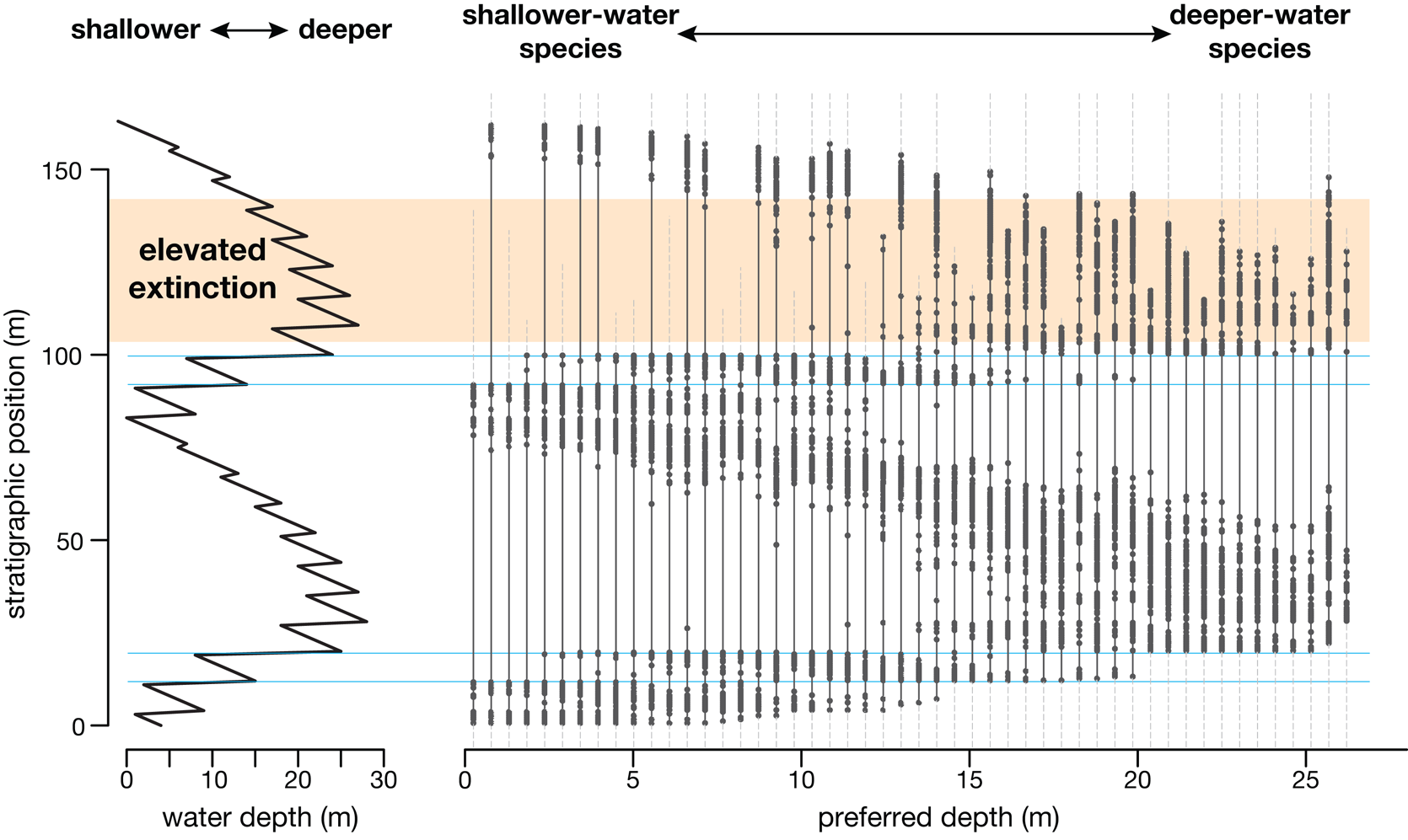
Finally, reconstructing the tempo of extinction from patterns of last occurrences has been an important implication of stratigraphic paleobiology (Holland and Patzkowsky Reference Holland and Patzkowsky2015; Holland Reference Holland2020; Zimmt et al. Reference Zimmt, Holland, Finnegan and Marshall2021). By leveraging the Po Plain dataset, Nawrot et al. (Reference Nawrot, Scarponi, Azzarone, Dexter, Kusnerik, Wittmer, Amorosi and Kowalewski2018) show that if a mass extinction occurred today, the fossil record of the Po Plain would produce a highly misleading picture of the extinction (Nawrot et al. Reference Nawrot, Scarponi, Azzarone, Dexter, Kusnerik, Wittmer, Amorosi and Kowalewski2018). Specifically, stratigraphically produced clusters of last occurrences arise that do not coincide with times of elevated extinction (Fig. 4). Their study has sobering implications for interpreting nearly all ancient extinction intervals.

Figure 4. Patterns of fossil occurrence through two transgressive–regressive sequences. The two sequences each contain 10 high-frequency parasequences, upward-shallowing cycles bounded by flooding surfaces across which water depth increases rapidly. Fifty species having the same peak abundance and depth tolerance but varying in preferred depth are shown sorted by their preferred depths. Dots depict fossil occurrences; solid lines show fossil ranges; and thin dashed gray lines show when species are extant (although possibly not preserved). Fossil occurrences systematically track changes in water depth, and major flooding surfaces (blue lines) have clusters of first and last occurrences. Note that the interval of elevated extinction does not have an obviously greater number of last occurrences. Most species that go extinct during the period of elevated extinction have their last occurrences at two major flooding surfaces immediately below the window of elevated extinction. Other last occurrences are spread through the elevated extinction interval and are not distinguishable from last occurrences caused by changing water depths. The full magnitude of the extinction would not be apparent until the next transgressive–regressive sequence (not shown). The timing of the extinction can be known only by studying correlative columns along the depositional dip.

Mass Extinctions and Recoveries

Determining the drivers of mass extinction and the timing of recoveries hinges on a careful and nuanced reading of the stratigraphic and fossil records to infer cause and effect. A careful reading of the records is crucial, because as the geologic timescale is refined and calibrated to a precision of a few tens of thousands of years, it is possible to estimate rates of processes at timescales thought to be impossible not that long ago. For these reasons, many studies collect and interpret data at the outcrop scale, commonly from single stratigraphic columns. Some have even advocated that mass extinctions are best studied in a single stratigraphic column (Lucas Reference Lucas2017). Yet it is precisely at the outcrop scale where interpreting the timing, tempo, and causes of mass extinction and recovery are potentially most fraught. Because stratigraphic paleobiological modeling studies of mass extinctions are so far limited to marine settings, our discussion will focus on the marine record.

Marine versus Nonmarine Systems

Until recently, the stratigraphic paleobiology of marine systems has been far better understood than that of nonmarine systems. This may partly reflect the substantial differences in fossil abundance (Regan et al. Reference Regan, Rogers and Holland2022) and, as a result, the generally greater ease with which large ecological datasets can be created with marine fossils. In addition, numerical models for generating hypotheses for shallow-marine systems have been well established for nearly 30 years (Holland Reference Holland1995, Reference Holland, Erwin and Wing2000, Reference Holland2020; Holland and Patzkowsky Reference Holland and Patzkowsky1999, Reference Holland and Patzkowsky2002, Reference Holland and Patzkowsky2015), whereas comparable models for fluvial systems have only recently been created (Holland and Loughney Reference Holland and Loughney2021; Holland Reference Holland2022b, Reference Holland2023). Comparable models for lacustrine, eolian, and other nonmarine systems have not yet been developed.

Architecture and Fossil Preservation

A key component of stratigraphic paleobiology is the recognition that patterns of fossil occurrences track the presence of particular sedimentary facies through stratigraphic successions. Organisms live in their preferred environments, and fossil occurrences in the rock record partly reflect these preferences (Patzkowsky and Holland Reference Patzkowsky and Holland2012).

However, only a limited portion of sedimentary environments and their inhabitants have the potential for preservation in the rock record. The taphonomic factors that contribute to the preservation and concentration of fossils are an important control on fossil occurrences. Some environments are unlikely to have a fossil record because they are unattractive habitats, such as sandy deserts for most plants and large vertebrates. Others are unlikely to have a fossil record because environmental conditions are not conducive to preservation of organic remains, such as acidic tropical forest soils (Behrensmeyer et al. Reference Behrensmeyer, Kidwell, Gastaldo, Erwin and Wing2000). The physical setting of sedimentary environments is also an important factor in their long-term preservation potential and greatly constrains the types of environments and biotas known in the rock record. For example, the record of high-elevation areas, caves, and deep-sea environments becomes progressively poorer into deep time.

Facies may lack a fossil record because they have low potential for fossil preservation. Preservation potential varies by environment and by organism, such that some environments have the potential to preserve a wide range of organisms (e.g., offshore transition, abandoned channels, stratified lakes), whereas others have low potential to preserve organic remains (e.g., rocky alluvial fans; Behrensmeyer and Hook Reference Behrensmeyer, Hook, Behrensmeyer, Damuth, DiMichele, Potts, Sues and Wing1992; Behrensmeyer et al. Reference Behrensmeyer, Kidwell, Gastaldo, Erwin and Wing2000; Holland and Loughney Reference Holland and Loughney2021). Even species that are abundant in a particular habitat may be underrepresented or absent in the fossil record because their remains are physically or chemically prone to alteration or decomposition in that environment (Behrensmeyer et al. Reference Behrensmeyer, Kidwell, Gastaldo, Erwin and Wing2000).

In marine settings, many facies are likely to preserve macroinvertebrates. Their hard parts and the fact that their remains contribute to the rock that preserves them result in fossil-rich accumulations that are tied to relative sea-level fluctuations (Kidwell Reference Kidwell, Allison and Briggs1991b). Marine communities also modify their environments through feedbacks that can be related to stratigraphic drivers. Models of hard-part accumulation in relation to sedimentation show how fossil concentrations form in response to stratigraphic controls and also through the biological response of fauna and the rates of shell production (Kidwell Reference Kidwell1985, Reference Kidwell1986; Tomašových et al. Reference Tomašových, Fürsich and Olszewski2006a, Reference Tomašových, Dominici, Nawrot, Zuschin, Nawrot, Dominici, Tomašových and Zuschin2023a). When sedimentation rate decreases relative to the input of skeletal material, burrowing infauna decrease and encrusting epifauna increase in abundance with the changing character of the microenvironment (Kidwell and Jablonski Reference Kidwell, Jablonski, Tevesz and McCall1983). When sedimentation rate increases relative to the input of skeletal material, the opposite trend occurs (Kidwell Reference Kidwell1985, Reference Kidwell1986). These feedbacks alter the environment by making it more attractive to encrusters with increasing skeletal input and more attractive to burrowers with decreasing skeletal input. In this way, the fauna of a given bathymetric zone can vary with the rates of terrigenous sediment input and shell production. Sediment mixing can also be an important control on the pattern of fossil occurrences at scales of centimeters to meters, depending on the depth of bioturbation (Tomašových et al. Reference Tomašových, Kidwell, Alexander and Kaufman2019).

In nonmarine settings, where fossil occurrences and concentrations are rare compared with marine systems, patterns of fossil occurrences tied to particular facies have long been noted (Behrensmeyer and Hook Reference Behrensmeyer, Hook, Behrensmeyer, Damuth, DiMichele, Potts, Sues and Wing1992; Holland and Loughney Reference Holland and Loughney2021). The occurrence of such facies can be stratigraphically controlled, although the larger geologic setting of different successions can yield differing patterns of fossil occurrences within facies (Behrensmeyer et al. Reference Behrensmeyer, Willis and Quade1995). For example, the preservation of fossil plants is strongly controlled by moisture, as well-drained sediments promote rapid aerobic respiration of organic matter, and plant fossils are typically known from a narrow range of facies representing lacustrine, swampy, or low-lying and wet environments (Behrensmeyer and Hook Reference Behrensmeyer, Hook, Behrensmeyer, Damuth, DiMichele, Potts, Sues and Wing1992; Gastaldo and Demko Reference Gastaldo, Demko, Allison and Bottjer2011). Vertebrate fossil preservation can be variable in facies that typically form in fluvial environments, and whether fossils occur in channel or floodplain facies may vary among sedimentary basins. Wet floodplain and abandoned-channel deposits are common settings for vertebrate preservation and have the potential to preserve rare taxa compared with better-drained floodplain deposits (Behrensmeyer Reference Behrensmeyer, Ethridge, Flores and Harvey1987; Therrien and Fastovsky Reference Therrien and Fastovsky2000; Loughney et al. Reference Loughney, Fastovsky and Parker2011). In some successions, channel deposits are the dominant setting for vertebrate assemblages, such as in the extensive Miocene Siwalik sequence of Pakistan (Badgley and Behrensmeyer Reference Badgley and Behrensmeyer1980; Behrensmeyer Reference Behrensmeyer, Ethridge, Flores and Harvey1987). In other nonmarine successions, bone concentrations are found predominantly in floodplain paleosols, such as in the Eocene Willwood Formation of Wyoming, USA (Bown and Kraus Reference Bown and Kraus1981), although it has been questioned whether this material accumulated on a soil surface or in sediment that was subsequently pedogenically modified (Rogers and Brady Reference Rogers and Brady2010).

The environment of deposition is important to fossil preservation, but subsequent landscape processes can determine the long-term preservation or architectural context of fossil occurrences. For example, plant fossil preservation is especially subject to subsequent landscape evolution and the position of the water table after deposition and burial (Gastaldo and Demko Reference Gastaldo, Demko, Allison and Bottjer2011). Plants that might have been initially buried in moist sediments that favor fossil preservation can be subsequently oxidized by a later fall in the position of the water table, which can prevent fossilization or result in lower-quality moldic preservation. The highest preservational potential occurs when accommodation and sedimentation increase following an episode of low or even negative rates of accommodation, and fossils are predicted to occur in such intervals, called expansion zones (sensu Martinsen et al. Reference Martinsen, Ryseth, Helland-Hansen, Flesche, Torkildsen and Idil1999). In the Cretaceous Two Medicine and Judith River Formations of Montana, fossiliferous concentrations occur along discontinuity surfaces that represent the reworking of previously deposited material from surrounding coastal plain facies (Rogers and Kidwell Reference Rogers and Kidwell2000). Interestingly, the probabilities of occurrence of invertebrate, plant, and vertebrate fossils do not differ among floodplain and channel facies of the Judith River Formation, although plant fossils are overall more abundant in deposits of the HAST than the LAST (Regan et al. Reference Regan, Rogers and Holland2022).

Where the constraints on fossil preservation are systematic, they can greatly affect not only the reconstructions of ancient environments and biota but also patterns of turnover and extinction. The fossil record of the Karoo Basin in South Africa is doubly affected by sparse facies bearing macroflora and their occurrence within condensed successions rife with lacunae (Gastaldo and Bamford Reference Gastaldo and Bamford2023). As a result, hiatuses and the greatly differing contexts of vertebrate and plant preservation create patterns of fossil occurrences that are stratigraphically governed yet misinterpreted as reflecting the history of the end-Permian extinction.

Large-Scale Architecture

The hierarchical nature of sequence-stratigraphic processes means that many of the concepts of stratigraphic paleobiology apply at a range of scales, from the outcrop to the continent. The major drivers of stratigraphic architecture (i.e., tectonic subsidence, climate and its control on sediment supply, eustatic sea level) can be detected at the basin scale but operate over wider areas and very long temporal ranges. As online resources have expanded, paleobiologists have been able to use extensive databases to evaluate patterns of stratigraphic architecture and fossil occurrences over greater distances and longer spans of time, as well as the long-term covariation of the rock and fossil records.

Sea-level cycles of varying scales and temporal durations are a well-known feature of the Phanerozoic rock record from which depositional sequences at all scales have been described (Sloss Reference Sloss1963). Sloss (Reference Sloss1976) considered the large-scale controls on the deposition and preservation of cratonic deposits through time as linked to a global mechanism unrelated to eustasy, presaging the concept of dynamic topography by mantle convection (Lovell Reference Lovell2010).

Raup (Reference Raup1976) was among the first to consider patterns of marine diversity in the fossil record as a function of the preservation of the Phanerozoic rock record. Although he considered sampling to account for the correlation of sedimentary rock area and volume and fossil diversity, subsequent workers have investigated the extent to which the fates of the rock and fossil records are linked and the large-scale processes that control them. For example, short-term patterns in diversity appear to be highly shaped by rock availability (Peters and Foote Reference Peters and Foote2001). Macrostratigraphy has greatly enabled the analysis of these questions by quantifying temporal changes in gap-bound rock packages, allowing them to be analyzed similarly to species’ ranges (Foote Reference Foote, Erwin and Wing2000; Peters Reference Peters2005, Reference Peters2006; Peters et al. Reference Peters, Quinn, Husson and Gaines2022). The Macrostrat database (Peters et al. Reference Peters, Husson and Czaplewski2018) has since evolved into an essential tool for quantitatively analyzing changes in the rock record over regional to continental scales, and its integration with the Paleobiology Database (PBDB; www.paleobiodb.org) enables fossil occurrence and diversity patterns to be analyzed within this framework.

Peters (Reference Peters2005) used these methods to evaluate the origination and extinction of marine sedimentary rock packages and marine animal genera over the Phanerozoic, showing them to be highly correlated. This strong correlation suggests that, while the fossil record is inherently linked to the rock record and the preservation of habitable facies, both records are shaped by similar drivers over large temporal and spatial scales; this is known as the common cause hypothesis (Peters Reference Peters2005; Peters et al. Reference Peters, Quinn, Husson and Gaines2022). Moreover, extinction rates of marine packages and genera in the Phanerozoic of North America are strongly correlated, whereas origination rates are not (Heim and Peters Reference Heim and Peters2011). This finding indicates that large-scale relationships between stratigraphic architecture and genus first and last occurrences differ from those observed and predicted at smaller scales (Holland Reference Holland1995; Peters and Heim Reference Peters and Heim2011), and common drivers may shape package truncations and biotic extinctions. Similarly, diversity and extinction of planktonic foraminifera in the Atlantic Ocean are highly correlated with the number of sedimentary packages, whereas origination is not (Peters et al. Reference Peters, Kelly and Fraass2013). This discrepancy suggests that a biological signal is being preserved, because a dominant stratigraphic control would be expected to affect origination, extinction, and diversity equally.

The correlation between package truncation and extinction rates highlights the importance of evaluating taxon last occurrences at a variety of scales and within a stratigraphic-paleobiological context (Heim and Peters Reference Heim and Peters2011; Holland and Patzkowsky Reference Holland and Patzkowsky2015). At the global scale, this approach has also been used to examine diversity in relation to supercycles of supercontinent formation and breakup (Zaffos et al. Reference Zaffos, Finnegan and Peters2017). The diversity of marine genera is correlated with increasing continental fragmentation through the Phanerozoic, particularly following the breakup of Rodinia and Pangaea. Intervals of low diversity correspond with coalescing continental movements, a relationship that may have contributed to the persistently low marine diversity through the early Mesozoic following the end-Permian extinction.

A macrostratigraphic approach also illuminates the occurrence of stromatolites (Peters et al. Reference Peters, Husson and Wilcots2017). Normalizing for rock volume shows stromatolites increasing in the Paleoproterozoic (ca. 2500 Ma), dominating through most of the Proterozoic (2500–800 Ma, and declining through the late Proterozoic (700–541 Ma). Moreover, despite the conventional wisdom that stromatolites increase in abundance following mass extinctions, a macrostratigraphic approach shows that stromatolite occurrence is not well correlated with times following mass extinctions. Lithologically, stromatolite occurrence is most strongly associated with dolomite, which may poorly preserve other fossils. Macrostratigraphy has also demonstrated the strong tie between the Cambrian explosion and the profound changes in geochemical cycling as the Great Unconformity was transgressed and buried (Peters and Gaines Reference Peters and Gaines2012; Peters et al. Reference Peters, Quinn, Husson and Gaines2022).

In the nonmarine record, macrostratigraphy can be used to understand diversity and landscape evolution in relation to tectonics and climate. For example, Loughney et al. (Reference Loughney, Badgley, Bahadori, Holt and Rasbury2021) evaluated changes in Neogene mammalian species richness in relation to sedimentation history during the tectonic evolution of the Basin and Range province in western North America. The history of sediment accumulation tracks landscape evolution over the formation of the Basin and Range and partly determines the timing of deposition of fossil-bearing sedimentary units. In contrast, spikes in species richness occurred during intervals of global warming, indicating that species’ responses to climate may be enhanced in topographically complex regions and are decoupled from preservation.

Assembly of Regional Ecosystems

At any time in Earth's history, global diversity is an amalgam of biogeographic provinces, latitudinal and elevational diversity gradients, and biodiversity hotspots and coolspots. Changes in global diversity over time must therefore reflect changes in this biogeographic structure, and the processes that control the spatial and temporal structure of diversity in local and regional ecosystems, such as origination, extinction, dispersal, and extirpation, are a major focus of research (Jablonski et al. Reference Jablonski, Roy and Valentine2006; Patzkowsky Reference Patzkowsky2017; Close et al. Reference Close, Benson, Saupe, Clapham and Butler2020; Saupe Reference Saupe2023).

The repeated deposition of sedimentary packages containing depth or elevation gradients provides a time–environment framework at subsequence scale necessary to study the main patterns, processes, and rates of change in regional diversity in deep time. With a time–environment framework, it is possible to evaluate the completeness of the environmental gradient, so that the absence of a taxon is interpreted as either a true absence or as missing due to a failure to preserve the preferred gradient position. Taxon occurrences outside the depositional basin indicate whether last occurrences represent true extinctions or extirpations, or likewise, whether first occurrences represent originations or immigrations. If the time–environment framework spans an environmental shift, the effect of the environmental change on the regional ecosystem can be evaluated, because the ecological gradient can be quantified before, during, and after the environmental shift (Patzkowsky and Holland Reference Patzkowsky and Holland2007; Dominici and Danise Reference Dominici, Danise, Nawrot, Dominici, Tomašových and Zuschin2022). In addition, it is possible to track individual taxa through time to test for niche conservatism and niche evolution (Holland and Zaffos Reference Holland and Zaffos2011).

Climate Change

Numerous studies document the effects of modern and ancient climate change on biotic community composition, evolution, and mass extinction. Climate is one important control on species distributions and stratigraphic architecture, although most studies investigating these relationships do not explicitly consider them from the perspective of stratigraphic paleobiology. Even so, there is great potential in studying climate-related patterns of biotic change using the principles of stratigraphic paleobiology.

Studies investigating the relationship between climate change and species diversity patterns yield variable results, underscoring that biodiversification events are commonly shaped by a “perfect storm” of contributing factors (Jablonski and Edie Reference Jablonski and Edie2023). For example, although the magnitude and rate of Phanerozoic temperature changes are positively correlated with marine animal extinction rates (Song et al. Reference Song, Kemp, Tian, Chu, Song and Dai2021), the extinction sensitivity of Phanerozoic marine invertebrates lacks a strong relationship with climate (Reddin et al. Reference Reddin, Kocsis and Kiessling2019). Global and regional analyses of mammalian diversity (Alroy et al. Reference Alroy, Koch, Zachos, Erwin and Wing2000; Barnosky and Carrasco Reference Barnosky and Carrasco2002) likewise show no strong relationship to climate change. Even so, mammalian faunal composition does track global climate trends (Figueirido et al. Reference Figueirido, Janis, Perez-Claros, de Renzi and Palmqvist2012). It is perhaps not surprising that something as extensive as the climate system should have unexpected or differing effects on biological systems, and there likely are aspects of the climate–biosphere connection that we either do not understand or cannot measure (Reddin et al. Reference Reddin, Kocsis and Kiessling2019). Moreover, recent climate changes demonstrate that local climate patterns need not track global patterns: for example, although global temperatures are currently increasing, the temperature of some regions is in net decline (Hansen et al. Reference Hansen, Ruedy, Sato and Lo2010). As such, analyzing regional biotic changes in light of regional rather than global climate proxies is essential (Raffi et al. Reference Raffi, Stanley and Marasti1985; Garilli Reference Garilli2011; Dominici et al. Reference Dominici, Benvenuti, Garilli, Uchman, Pollina and David2020; Borghi and Garilli Reference Borghi and Garilli2022). Similarly, marine-derived paleoclimate proxies do not necessarily reflect nonmarine climate, which may explain some discrepancies among climate and nonmarine diversity patterns (Alroy et al. Reference Alroy, Koch, Zachos, Erwin and Wing2000).

The availability of global climate-proxy datasets allows large-scale analyses with diversity data from the PBDB. For most analyses involving Cenozoic climate, Zachos et al. (Reference Zachos, Pagani, Sloan, Thomas and Billups2001) has been the favored source, with Westerhold et al. (Reference Westerhold, Marwan, Drury, Liebrand, Agnini, Anagnostou and Barnet2020) ascending with updated records; Veizer and Prokoph (Reference Veizer and Prokoph2015) and Scotese et al. (Reference Scotese, Song, Mills and van der Meer2021) provide reconstructions spanning the Phanerozoic. Although these are useful and powerful resources for investigating change through time, the patterns cannot necessarily be taken at face value. A stratigraphic paleobiological perspective that considers the spatial distribution of sedimentary basins and their intersections with biomes and provinces is crucial for understanding how the record is assembled and how it can be interpreted (Holland Reference Holland2016). Similarly, studies should reflect the implications of the large-scale selectivity of the fossil record, such as the dominance of low-elevation habitats in the nonmarine fossil record and the preferential preservation of particular shallow-marine habitats (Nyberg and Howell Reference Nyberg and Howell2015, Reference Nyberg and Howell2016; Holland et al. Reference Holland, Loughney and Cone2023).

For large-scale analyses of climate and biodiversity, macrostratigraphy provides an opportunity to investigate the coupled effects of changing climate on diversity, sea level, and rock availability (Peters et al. Reference Peters, Quinn, Husson and Gaines2022). For example, Late Ordovician extinction and sedimentary packages appear to be jointly driven by climate and eustasy (Finnegan et al. Reference Finnegan, Heim, Peters and Fischer2012). This approach may also be useful in establishing other biological correlates of climate change, such as ecological and functional traits.

Geochemistry and Stratigraphic Paleobiology

Global geochemical proxies of environmental conditions are often matched against fossil occurrences to infer environmental causes of extinction (e.g., Saltzman et al. Reference Saltzman, Edwards, Adrain and Westrop2015), often with little consideration of how stratigraphic architecture affects fossil occurrences. Even so, geochemical proxies are also affected by variation in sedimentation rates, facies variability, and hiatuses, just as are fossil occurrences (Railsback et al. Reference Railsback, Holland, Hunter, Jordan, Diaz and Crowe2003; Trampush and Hajek Reference Trampush and Hajek2017; Hay et al. Reference Hay, Creveling, Hagen, Maloof and Huybers2019; Pulsipher et al. Reference Pulsipher, Schiffbauer, Jeffrey, Huntley, Fike and Shelton2021; Prave et al. Reference Prave, Kirsimäe, Lepland, Fallick, Kreitsmann, Deines and Romashkin2022), so they cannot be interpreted as literal indicators of the timing and intensity of environmental change. Subaerial exposure and diagenesis are additional sources of variability in proxy records. Studies of modern carbonate environments indicate that the variability among facies in δ¹³C values of carbonate sediment grains equals that seen in the deep-time record (Geyman and Maloof Reference Geyman and Maloof2021). Simulated stratigraphic sections using these modern values show abrupt jumps in δ¹³C values across facies shifts at flooding surfaces. In the deep-time record, δ¹³C shifts at flooding surfaces would be expected to co-occur with clusters of first or last occurrences, and this could easily be misinterpreted as a cause-and-effect relationship rather than just the expectation across abrupt shifts in facies. On the other hand, fossil occurrences and geochemical proxies may not respond similarly to environmental gradients, so that even if a specific environmental shift caused an extinction, it may not coincide stratigraphically with fossil occurrences in a way that permits an interpretation as simple cause and effect.

Integrating local environmental proxies with fossil occurrences in measured stratigraphic sections holds promise for making direct inferences about environmental causes of extinction. For example, marine anoxia likely contributed to many regional extinctions in the geologic past, and its effects on benthic organisms should be observable. However, the expansion of ancient marine anoxic zones is often marked by the appearance of black shales at a flooding surface. As a result, the coincident extinction of shallow-water taxa cannot be confirmed until those taxa can be shown to be absent in shallow-water facies above the flooding surface. Geochemical proxies of local seafloor anoxia can help identify oxygen fluctuations where facies do not change substantially (Pruss et al. Reference Pruss, Jones, Fike, Tosca and Wignall2019). Pairing geochemical proxies for local marine anoxia with fossil occurrences in a time–environment framework built on depositional sequences could reveal the direct effects of seafloor oxygen fluctuations on benthic communities. Similar studies integrating stratigraphic paleobiology and geochemistry are needed to test for specific oceanographic or climatic variables as causes of extinction.

Phylogenetics and Stratigraphic Paleobiology

Phylogenetic methods are central to many of the basic questions in evolutionary paleoecology surrounding the origin, diversification, and environmental distribution of clades. Phylogenetic trees scaled against geologic time can be used to estimate rates of speciation, extinction, and morphological evolution. Adding information about abundance and habitat preference allows an evaluation of how rates of diversification and morphological evolution are determined by environment (Ricklefs Reference Ricklefs2006; Lamsdell et al. Reference Lamsdell, Congreve, Hopkins, Krug and Patzkowsky2017). Stratigraphic paleobiological principles can support and enhance phylogenetic studies in two important ways. First, estimating the time of origin and rates of speciation and extinction in diversifying clades is based on the record of species’ first and last occurrences. Early development of phylogenetic models to make these estimates were based on simplistic assumptions of fossil recovery, specifically uniform preservation rates (Barido-Sottani et al. Reference Barido-Sottani, Pett, O'Reilly and Warnock2019). Fossil recovery is demonstrably nonuniform on both short timescales (<10 Myr), where fossil recovery is controlled by stratigraphic architecture and environmental distributions of species (Patzkowsky and Holland Reference Patzkowsky and Holland2012), and longer timescales (>10 Myr), where fossil recovery is controlled by tectonic processes that construct and destroy sedimentary basins (Holland Reference Holland2016). Models incorporating more realistic fossil recovery rates based on stratigraphic architecture are needed (e.g., Barido-Sottani et al. Reference Barido-Sottani, Pett, O'Reilly and Warnock2019). Case studies of specific clades should utilize empirical estimates of fossil preservation using databases of fossil and lithologic occurrences, such as the PBDB and Macrostrat (Wagner and Marcot Reference Wagner and Marcot2013; Congreve et al. Reference Congreve, Patzkowsky and Wagner2021).

Second, phylogenies of diversifying clades can be mapped onto the time–environment framework provided by a stratigraphic-paleobiological approach. Doing this would help explain, for example, the distribution of niche conservatism and niche expansion among subclades in maintaining environmental gradients in diversity (Sepkoski Reference Sepkoski1991; Jablonski et al. Reference Jablonski, Roy and Valentine2006; Ricklefs Reference Ricklefs2006; Tomašových et al. Reference Tomašových, Dominici, Zuschin and Merle2014). Merging phylogenetics with stratigraphic paleobiology promises to accelerate progress in understanding the ecological and evolutionary processes of clade origin and diversification and the assembly of regional biotas in an environmental context.

Large-Scale Structure of the Fossil Record

The PBDB has permitted extraordinary insight into long-term and large-scale patterns in the fossil record for more than 20 years. A principal challenge to interpreting the biological meaning of this archive is coming to terms with the temporal and geographic inhomogeneities in the data. Despite substantial efforts by an ever-growing number of paleontologists, large portions of the published fossil record have not been entered, and the PBDB remains an uneven sampling of the known fossil record (Ye and Peters Reference Ye and Peters2023). At large scales (global, Phanerozoic), the hope is that the sampling is even enough that patterns are biologically meaningful, but at smaller geographic and shorter temporal scales, uneven sampling of the known record becomes more of a concern.

Even if these effects were overcome by an exhaustive catalogue of the known fossil record, the inference of biological meaning to patterns in the PBDB must increasingly hinge on a stratigraphic-paleobiological outlook, specifically that even over large spatial (basin to globe) and temporal (tens to hundreds of millions of years) scales, the fossil record is systematically structured by how the stratigraphic record is constructed. Macrostratigraphy offers the most promise at these scales (Peters et al. Reference Peters, Quinn, Husson and Gaines2022).

One such challenge is the global temporal correlation in the available stratigraphic record. For example, Ager (Reference Ager1973) pointed out the lateral persistence of facies—that certain facies are extraordinarily widespread at particular times in Earth's history, such as Upper Cretaceous chalk, Tithonian limestone, Pennsylvanian coal, and Mississippian limestone, and many others. Although this partly reflects global climate and the configuration of continents, it must be remembered that the presence of some facies implies that others must have existed. For example, Upper Devonian black shales are widespread across North America, yet the presence of these offshore shales implies that coastal marine environments must also have existed. Owing to their subsequent erosion or inaccessibility, it may be impossible to sample them (Smith et al. Reference Smith, Gale and Monks2001), and as a result, the regional Late Devonian drop in diversity may be largely a reflection of the facies available for study. This can be addressed only by considering the nature of the available (and sampled) stratigraphic record. Similarly, the formation of sedimentary basins—and the types of basins, which differ greatly in their extent and life spans—is likely to be highly correlated through geologic time, owing to global cycles in supercontinent formation and breakup (Holland Reference Holland2016). This not only affects global and continental diversity (Holland Reference Holland2018), but it also affects what life can be preserved as fossils and where that can happen (Holland Reference Holland2016). Because of these global correlations, it can be difficult to distinguish whether patterns in the fossil record represent what has been preserved in the stratigraphic record or patterns in the history of life (Miller Reference Miller, Erwin and Wing2000). A promising area of investigation is understanding how the history of life—particularly biogeography—is driven by plate tectonics (e.g., Holland Reference Holland2018; Jablonski and Edie Reference Jablonski and Edie2023), but also how the formation and cessation of sedimentary basins selectively preserve this history of life (Holland Reference Holland2016; Holland et al. Reference Holland, Loughney and Cone2023). A stratigraphic paleobiological perspective at these wide spatial and long temporal scales offers the best chance for extracting the history of life from the fossil record.