


1. Introduction
Turbulence is composed of blobs of fluid, called eddies, over which velocity fluctuations are highly correlated. These eddies span a broad range of sizes, and the distribution of turbulent kinetic energy across the range of eddy sizes is a critical attribute of a turbulent flow. We focus on the following question: How do we quantify this energy distribution? In other words, we need an energy-density function.
The standard approach to quantifying the distribution of energy is to introduce the spectral tensor,
 $\Phi _{ij}(\boldsymbol{k})$
, which is the Fourier transform of the two-point velocity correlation tensor
$\Phi _{ij}(\boldsymbol{k})$
, which is the Fourier transform of the two-point velocity correlation tensor
 $Q_{ij}(\boldsymbol{r}):=\langle {u_{i}(\boldsymbol{x})u_{j}(\boldsymbol{x}+\boldsymbol{r})}\rangle$
 \begin{align}& \Phi _{ij}(\boldsymbol{k})=\frac {1}{(2\pi )^{3}}\int _{\mathbb{R}^{3}}d^{3}\boldsymbol{r}Q_{ij}(\boldsymbol{r})e^{-\textrm{i}\boldsymbol{k}\boldsymbol{\cdot }\boldsymbol{r}}, \end{align}
 \begin{align}&\quad\,\,\, Q_{ij}(\boldsymbol{r})=\int _{\mathbb{R}^{3}}d^{3}\boldsymbol{k}\Phi _{ij}(\boldsymbol{k})e^{\textrm{i}\boldsymbol{k}\boldsymbol{\cdot }\boldsymbol{r}} , \end{align}
where
 $\boldsymbol{x}$
and
$\boldsymbol{x}$
and
 $\boldsymbol{x}+\boldsymbol{r}$
are position vectors,
$\boldsymbol{x}+\boldsymbol{r}$
are position vectors,
 $\boldsymbol{k}$
is the wavenumber corresponding to
$\boldsymbol{k}$
is the wavenumber corresponding to
 $\boldsymbol{r}$
,
$\boldsymbol{r}$
,
 $\boldsymbol{u}$
is the turbulent velocity vector, the subscript indices denote Cartesian components of the corresponding vector or tensor and
$\boldsymbol{u}$
is the turbulent velocity vector, the subscript indices denote Cartesian components of the corresponding vector or tensor and
 $\langle \rangle$
denotes an ensemble average. Note that we have assumed the turbulent flow to be homogeneous (i.e. its statistical properties are independent of
$\langle \rangle$
denotes an ensemble average. Note that we have assumed the turbulent flow to be homogeneous (i.e. its statistical properties are independent of
 $\boldsymbol{x}$
). In this study, we shall restrict attention to homogeneous turbulence. When the turbulent flow is homogeneous and isotropic, we can introduce the three-dimensional spectral energy-density function,
$\boldsymbol{x}$
). In this study, we shall restrict attention to homogeneous turbulence. When the turbulent flow is homogeneous and isotropic, we can introduce the three-dimensional spectral energy-density function,
 $E(k)$
, by integrating
$E(k)$
, by integrating
 $({1}/{2})\Phi _{ii}(\boldsymbol{k})$
over a spherical shell,
$({1}/{2})\Phi _{ii}(\boldsymbol{k})$
over a spherical shell,
 $\mathcal{S}(k)$
, of radius
$\mathcal{S}(k)$
, of radius
 $k= \| {\boldsymbol k}\|$
The factor of
 ${1}/{2}$
was introduced to obtain the energy constraint
${1}/{2}$
was introduced to obtain the energy constraint
 \begin{align} \frac {1}{2}\langle {\boldsymbol{u}^{2}}\rangle &=\int _{0}^{\infty }{\textrm d}kE(k), \end{align}
which follows from (1.1b
) and the relations
 $Q_{ii}(r = 0)=\langle {\boldsymbol{u}^{2}}\rangle$
and
$Q_{ii}(r = 0)=\langle {\boldsymbol{u}^{2}}\rangle$
and
 $Q_{ii}(r \rightarrow \infty )=0$
, where
$Q_{ii}(r \rightarrow \infty )=0$
, where
 $r=\|\boldsymbol{r}\|$
. (For simplicity of notation, in this study, we use the same symbol to represent a function whether its argument is a vector, e.g.
$r=\|\boldsymbol{r}\|$
. (For simplicity of notation, in this study, we use the same symbol to represent a function whether its argument is a vector, e.g.
 $\boldsymbol{r}$
, or its scalar norm,
$\boldsymbol{r}$
, or its scalar norm,
 $r$
). The energy constraint underpins the role of
$r$
). The energy constraint underpins the role of
 $E(k)$
as an energy-density function. Specifically, it implies that
$E(k)$
as an energy-density function. Specifically, it implies that
 ${\textrm d}kE(k)$
is the contribution to
${\textrm d}kE(k)$
is the contribution to
 $({1}/{2})\langle {\boldsymbol{u}^{2}}\rangle$
(which is the turbulent kinetic energy) from wavenumber modes in the range
$({1}/{2})\langle {\boldsymbol{u}^{2}}\rangle$
(which is the turbulent kinetic energy) from wavenumber modes in the range
 $(k,k+{\textrm d}k)$
so that the function
$(k,k+{\textrm d}k)$
so that the function
 $E(k)$
represents the energy density in the spectral space. But the problem here is how to interpret
$E(k)$
represents the energy density in the spectral space. But the problem here is how to interpret
 $k$
in terms of eddies. Although, as a rule of thumb, we may loosely associate
$k$
in terms of eddies. Although, as a rule of thumb, we may loosely associate
 $k^{-1}$
with the eddy size, because eddies are not waves, the validity of such one-to-one association is unclear.
$k^{-1}$
with the eddy size, because eddies are not waves, the validity of such one-to-one association is unclear.
These difficulties underscore the need for a complementary approach; see Davidson (Reference Davidson2004, Ch. 6) for a detailed discussion of this topic. In the real space, the analogue of
 $E(k)$
is a spatial energy-density function,
$E(k)$
is a spatial energy-density function,
 $V\!(r)$
. In analogy with the properties of
$V\!(r)$
. In analogy with the properties of
 $E(k)$
, we can require
$E(k)$
, we can require
 $V\!(r)$
to have the following characteristic properties (Davidson Reference Davidson2004):
$V\!(r)$
to have the following characteristic properties (Davidson Reference Davidson2004):
-
(i)
 $ V\!(r) \geqslant 0$
;
$ V\!(r) \geqslant 0$
; -
(ii)
$ \int _{0}^{\infty }{\textrm d}rV\!(r) = ({1}/{2})\langle {\boldsymbol{u}^{2}}\rangle$
; -
(iii) for a random distribution of eddies of fixed size
$\ell _{e}$
, the corresponding
$V\!(r)$
manifests a clear peak around
$r \sim \ell _{e}$
.


An insightful approach to obtain
 $V\!(r)$
was pioneered by Townsend (Reference Townsend1976). Unlike the case in the spectral space, where linking
$V\!(r)$
was pioneered by Townsend (Reference Townsend1976). Unlike the case in the spectral space, where linking
 $k^{-1}$
with eddy size is unclear, he sought to construct a function in the real space whose magnitude for the argument
$k^{-1}$
with eddy size is unclear, he sought to construct a function in the real space whose magnitude for the argument
 $r$
is clearly related to the energy of eddies of ‘diameter’
$r$
is clearly related to the energy of eddies of ‘diameter’
 $r$
. For that purpose, he used Kolmogorov’s two-point velocity structure function (Kolmogorov Reference Kolmogorov1941)
$r$
. For that purpose, he used Kolmogorov’s two-point velocity structure function (Kolmogorov Reference Kolmogorov1941)
 \begin{align} S_{ij}(\boldsymbol{r}):=\langle {{ [ u_{i}(\boldsymbol{x})-u_{i}(\boldsymbol{x}+\boldsymbol{r}) ]}{[ u_{j}(\boldsymbol{x})-u_{j}(\boldsymbol{x}+\boldsymbol{r}) ]}}\rangle . \end{align}
Consider the velocity component directed along
 $\boldsymbol{r} = r \boldsymbol{\hat e}_{1}$
. Heuristically, it is argued that
$\boldsymbol{r} = r \boldsymbol{\hat e}_{1}$
. Heuristically, it is argued that
 $S_{11}(r)$
is dominated by contributions from eddies of size
$S_{11}(r)$
is dominated by contributions from eddies of size
 $r$
or less. This is because eddies of size
$r$
or less. This is because eddies of size
 $r$
or greater make comparable contributions to both
$r$
or greater make comparable contributions to both
 $u_{1}(\boldsymbol{x})$
and
$u_{1}(\boldsymbol{x})$
and
 $u_{1}(\boldsymbol{x}+\boldsymbol{r})$
, and thus contribute little to
$u_{1}(\boldsymbol{x}+\boldsymbol{r})$
, and thus contribute little to
 $S_{11}(r)$
. With this picture in mind, he postulated that the contribution to
$S_{11}(r)$
. With this picture in mind, he postulated that the contribution to
 $\langle {u_{1}^{2}}\rangle$
from eddies of size
$\langle {u_{1}^{2}}\rangle$
from eddies of size
 $r$
in unit range of
$r$
in unit range of
 $\log r$
is
$\log r$
is
 \begin{align} -r\frac {\partial }{\partial r}{\left [ \frac {1}{2} S_{11}(r) \right ]}. \end{align}
Notably, Townsend did not obtain an explicit expression for
 $V\!(r)$
from (1.5). That task was taken up only relatively recently.
$V\!(r)$
from (1.5). That task was taken up only relatively recently.
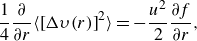
Davidson (Reference Davidson2004) argued that Townsend’s proposal leads to
 \begin{align} V_{\textit{TD}}(r)&:=\frac {\partial }{\partial r}{\left [ \frac {3}{4}\langle {[\Delta \upsilon (r)]^{2}}\rangle \right ]}, \end{align}
where
 $\langle {{ [ \Delta \upsilon (r) ]}^{2}}\rangle$
is the longitudinal structure function, which is defined as
$\langle {{ [ \Delta \upsilon (r) ]}^{2}}\rangle$
is the longitudinal structure function, which is defined as
 \begin{align} \langle {{\left [ \Delta \upsilon (r) \right ]}^{2}}\rangle &:=S_{ij}\frac {r_{i}r_{j}}{r^{2}}. \end{align}
We shall refer to
 $V_{\textit{TD}}(r)$
as the Townsend–Davidson function. On the other hand, Hamba (Reference Hamba2015) postulated
$V_{\textit{TD}}(r)$
as the Townsend–Davidson function. On the other hand, Hamba (Reference Hamba2015) postulated
 \begin{align} V_{\textit{TH}}(r)&:=-\frac {\partial }{\partial r}\frac {1}{2}Q_{ii}(r), \end{align}
which we shall refer to as the Townsend–Hamba function. (Note that
 $V_{\textit{TH}}(r)$
is closely related to equation (13) of Danaila, Antonia & Burattini (Reference Danaila, Antonia and Burattini2012).) Surprisingly, although they stem from the same proposal, the expressions for
$V_{\textit{TH}}(r)$
is closely related to equation (13) of Danaila, Antonia & Burattini (Reference Danaila, Antonia and Burattini2012).) Surprisingly, although they stem from the same proposal, the expressions for
 $V_{\textit{TD}}(r)$
and
$V_{\textit{TD}}(r)$
and
 $V_{\textit{TH}}(r)$
are distinct.
$V_{\textit{TH}}(r)$
are distinct.
Inspired by Davidson (Reference Davidson2004) and Hamba (Reference Hamba2015), we take a fresh look at deriving
 $V\!(r)$
. We first discuss homogeneous isotropic turbulence, and then generalise our approach to anisotropic flows. Thereafter, we draw attention to an important point that has not been explicitly considered before. Analogous to the well-known one-dimensional spectral energy-density functions, we introduce one-dimensional spatial energy-density functions. This allows us to resolve the surprising discrepancies between (1.6) and (1.8). Moreover, the one-dimensional functions may find particular appeal for the analysis of empirical data. We demonstrate this point with a few illustrative examples.
$V\!(r)$
. We first discuss homogeneous isotropic turbulence, and then generalise our approach to anisotropic flows. Thereafter, we draw attention to an important point that has not been explicitly considered before. Analogous to the well-known one-dimensional spectral energy-density functions, we introduce one-dimensional spatial energy-density functions. This allows us to resolve the surprising discrepancies between (1.6) and (1.8). Moreover, the one-dimensional functions may find particular appeal for the analysis of empirical data. We demonstrate this point with a few illustrative examples.
2. Deriving
$\boldsymbol{V}\!(\boldsymbol{r})$
for homogeneous isotropic turbulence

In the spectral space, the energy constraint of (1.3) underpins the interpretation of
 $E(k)$
as an energy-density function. Here, we derive
$E(k)$
as an energy-density function. Here, we derive
 $V\!(r)$
for homogeneous isotropic turbulence using a spatial analogue of the energy constraint. (In Appendix A, we derive this expression using Townsend’s approach).
$V\!(r)$
for homogeneous isotropic turbulence using a spatial analogue of the energy constraint. (In Appendix A, we derive this expression using Townsend’s approach).
From the sifting property of the Dirac delta function
 $\delta (r)$
, we can write
$\delta (r)$
, we can write
 \begin{align} \frac {1}{2}Q_{ii}(r) &=\int _{0}^{\infty }{\textrm d}r^{\prime }{\left [ \frac {1}{2}Q_{ii}(r^{\prime }) \right ]} \delta (r^{\prime }-r). \end{align}
By introducing the Heaviside function
 $\Theta (r)$
, the above integral can be expressed as
$\Theta (r)$
, the above integral can be expressed as
 \begin{align} \frac {1}{2}Q_{ii}(r) &=\int _{0}^{\infty }{\textrm d}r^{\prime }{\left [ \frac {1}{2}Q_{ii}(r^{\prime }) \right ]} \frac {\partial }{\partial r^{\prime }}\Theta (r^{\prime }-r),\nonumber \\ &=\int _{0}^{\infty }{\textrm d}r^{\prime }\frac {\partial }{\partial r^{\prime }}{\left [ -\frac {1}{2}Q_{ii}(r^{\prime }) \right ]} \Theta (r^{\prime }-r),\quad (\text{integration by parts})\nonumber \\ &=\int _{r}^{\infty }{\textrm d}r^{\prime }\frac {\partial }{\partial r^{\prime }}{\left [ -\frac {1}{2}Q_{ii}(r^{\prime }) \right ]}, \end{align}
where we have used
 $Q_{ii}(r\to \infty ) = 0$
. Taking the limit
$Q_{ii}(r\to \infty ) = 0$
. Taking the limit
 $r\to 0$
and noting
$r\to 0$
and noting
 $Q_{ii}(0) = \langle {\boldsymbol{u}^{2}}\rangle$
, we have
$Q_{ii}(0) = \langle {\boldsymbol{u}^{2}}\rangle$
, we have
 \begin{align} \int _{0}^{\infty } {\textrm d}r^{\prime }{\left [ -\frac {\partial }{\partial r^{\prime }}\frac {1}{2}Q_{ii}(r^{\prime }) \right ]}&= \frac {1}{2}\langle {\boldsymbol{u}^{2}}\rangle , \end{align}
which is a real-space analogue of the spectral-space energy constraint, (1.3). Thus, analogous to the three-dimensional spectral energy-density function,
 $E(k)$
, we can define a three-dimensional spatial energy-density function
$E(k)$
, we can define a three-dimensional spatial energy-density function
 \begin{align} V\!(r)&:=-\frac {\partial }{\partial r}\frac {1}{2}Q_{ii}(r), \end{align}
which is the Townsend–Hamba function,
 $V_{\textit{TH}}(r)$
(1.8).
$V_{\textit{TH}}(r)$
(1.8).
Some additional remarks may be useful. Although we could have derived (2.4) without (2.2), introducing (2.2) allows us to interpret
 $Q_{ii}(r)$
in terms of kinetic energy of eddies. Combining (2.2) and (2.4), we get
$Q_{ii}(r)$
in terms of kinetic energy of eddies. Combining (2.2) and (2.4), we get
 \begin{align} \frac {1}{2}Q_{ii}(r)&=\int _{r}^{\infty } {\textrm d}s\, V\!(s)=\int _{0}^{\infty } {\textrm d}s\, V\!(s)\Theta (s-r). \end{align}
Here, the ideal low-pass filter
 $\Theta (r)$
ensures that only eddies of size
$\Theta (r)$
ensures that only eddies of size
 $r$
or greater make contributions to
$r$
or greater make contributions to
 $({1}/{2})Q_{ii}(r)$
, with the implication
$({1}/{2})Q_{ii}(r)$
, with the implication
 \begin{align} \frac {1}{2}Q_{ii}(r)= [ \textrm {cumulative kinetic energy held in eddies of size }r\textrm { or greater} ]. \end{align}
This interpretation based on
 $V\!(r)$
can be contrasted with that based on
$V\!(r)$
can be contrasted with that based on
 $E(k)$
. We can express
$E(k)$
. We can express
 $Q_{ii}(r)$
in terms of
$Q_{ii}(r)$
in terms of
 $E(k)$
as
$E(k)$
as
 \begin{align} \frac {1}{2}Q_{ii}(r)&=\int _{0}^{\infty } {\textrm d}k\, E(k)\frac {\sin (kr)}{kr}. \end{align}
Note that, while
 $\sin (kr)/(kr)$
effectively is a low pass-filter, dominated by contributions from wavenumbers
$\sin (kr)/(kr)$
effectively is a low pass-filter, dominated by contributions from wavenumbers
 $k\lesssim 1/r$
, it is not an ideal filter and has an infinite extent in
$k\lesssim 1/r$
, it is not an ideal filter and has an infinite extent in
 $k$
-space. Thus, all Fourier modes contribute to
$k$
-space. Thus, all Fourier modes contribute to
 $({1}/{2})Q_{ii}(r)$
. Interpreting the Fourier modes as eddy sizes implies that eddies of all sizes contribute to
$({1}/{2})Q_{ii}(r)$
. Interpreting the Fourier modes as eddy sizes implies that eddies of all sizes contribute to
 $({1}/{2})Q_{ii}(r)$
. The above discussion underscores how different definitions of the energy-density function embody distinct physical interpretations; also see Davidson (Reference Davidson2004).
$({1}/{2})Q_{ii}(r)$
. The above discussion underscores how different definitions of the energy-density function embody distinct physical interpretations; also see Davidson (Reference Davidson2004).
3. Deriving
$\boldsymbol{V}\!(\boldsymbol{r})$
for homogeneous anisotropic turbulence

So far, we have focused on homogeneous isotropic turbulence. Next we generalise the analysis of § 2 for homogeneous anisotropic turbulence and derive an expression for the three-dimensional spatial energy-density function,
 $V\!(\boldsymbol{r})$
.
$V\!(\boldsymbol{r})$
.
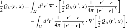
We begin with extending (2.1) for the general case (without assuming isotropy or homogeneity)
 \begin{align} \frac {1}{2}Q_{ii}(\boldsymbol{r},\boldsymbol{x})&=\int _{\Omega }d^{3}\boldsymbol{r}^{\prime } {\left [ \frac {1}{2}Q_{ii}(\boldsymbol{r}^{\prime },\boldsymbol{x}) \right ]} \delta ^{3}(\boldsymbol{r}^{\prime }-\boldsymbol{r}), \end{align}
where
 $\Omega$
is any arbitrary flow domain (with the restriction that
$\Omega$
is any arbitrary flow domain (with the restriction that
 $\boldsymbol{r}$
is contained within it) and
$\boldsymbol{r}$
is contained within it) and
 $\delta ^{3}(\boldsymbol{r})$
denotes the Dirac delta function in
$\delta ^{3}(\boldsymbol{r})$
denotes the Dirac delta function in
 $\mathbb{R}^{3}$
. Noting that the Dirac delta function satisfies the relation
$\mathbb{R}^{3}$
. Noting that the Dirac delta function satisfies the relation
 \begin{align} \nabla \boldsymbol{\cdot }{{\left [ \left(\frac {1}{4\pi }\frac {\boldsymbol{r}-\boldsymbol{r}^{\prime }} {{\left ||\boldsymbol{r}-\boldsymbol{r}^{\prime }\right |\!|}^{3}}\right) \right ]}}&=\delta ^{3}(\boldsymbol{r}-\boldsymbol{r}^{\prime }), \end{align}
we write (3.1) as
 \begin{align} \frac {1}{2}Q_{ii}(\boldsymbol{r},\boldsymbol{x})&=\int _{\Omega }d^{3}\boldsymbol{r}^{\prime }\, \boldsymbol{\nabla }^{\prime }\boldsymbol{\cdot }{\left [ \frac {1}{2}Q_{ii}(\boldsymbol{r}^{\prime },\boldsymbol{x}) \frac {1}{4\pi }\frac {\boldsymbol{r}^{\prime }-\boldsymbol{r}}{{\left ||\boldsymbol{r}^{\prime }-\boldsymbol{r}\right |\!|}^{3}} \right ]}\nonumber \\ &\quad -\int _{\Omega }d^{3}\boldsymbol{r}^{\prime }\, \frac {1}{4\pi }\frac {\boldsymbol{r}^{\prime }-\boldsymbol{r}}{{\left ||\boldsymbol{r}^{\prime }-\boldsymbol{r}\right |\!|}^{3}} \boldsymbol{\cdot }\boldsymbol{\nabla }^{\prime } {\left [ \frac {1}{2}Q_{ii}(\boldsymbol{r}^{\prime },\boldsymbol{x}) \right ]} .\end{align}
Applying the divergence theorem yields
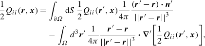 \begin{align} \frac {1}{2}Q_{ii}(\boldsymbol{r},\boldsymbol{x})&=\int _{\partial \Omega }{\textrm d}S\, \frac {1}{2}Q_{ii}(\boldsymbol{r}^{\prime },\boldsymbol{x}) \frac {1}{4\pi }\frac {(\boldsymbol{r}^{\prime }-\boldsymbol{r})\boldsymbol{\cdot }\boldsymbol{n}^{\prime }}{{\left ||\boldsymbol{r}^{\prime }-\boldsymbol{r}\right |\!|}^{3}}\nonumber \\ &\quad -\int _{\Omega }d^{3}\boldsymbol{r}^{\prime }\, \frac {1}{4\pi }\frac {\boldsymbol{r}^{\prime }-\boldsymbol{r}}{{\left ||\boldsymbol{r}^{\prime }-\boldsymbol{r}\right |\!|}^{3}} \boldsymbol{\cdot }\boldsymbol{\nabla }^{\prime } {\left [ \frac {1}{2}Q_{ii}(\boldsymbol{r}^{\prime },\boldsymbol{x}) \right ]}, \end{align}
where
 $\hat{\boldsymbol{n}}^{\prime }$
is the unit normal to the surface
$\hat{\boldsymbol{n}}^{\prime }$
is the unit normal to the surface
 $\partial \Omega$
that bounds the domain
$\partial \Omega$
that bounds the domain
 $\Omega$
. This brings us to a critical consideration. When the turbulence is homogeneous, the surface integral in (3.4) vanishes, yielding
$\Omega$
. This brings us to a critical consideration. When the turbulence is homogeneous, the surface integral in (3.4) vanishes, yielding
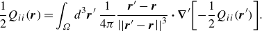 \begin{align} \frac {1}{2}Q_{ii}(\boldsymbol{r})&= \int _{\Omega }d^{3}\boldsymbol{r}^{\prime }\, \frac {1}{4\pi }\frac {\boldsymbol{r}^{\prime }-\boldsymbol{r}}{{\left ||\boldsymbol{r}^{\prime }-\boldsymbol{r}\right |\!|}^{3}} \boldsymbol{\cdot }\boldsymbol{\nabla }^{\prime }{\left [ -\frac {1}{2}Q_{ii}(\boldsymbol{r}^{\prime }) \right ]}. \end{align}
This is the generalisation of (2.2) for homogeneous anisotropic turbulence.
Next, taking the limit
 $\boldsymbol{r}\to \boldsymbol{0}$
, we arrive at the energy constraint
$\boldsymbol{r}\to \boldsymbol{0}$
, we arrive at the energy constraint
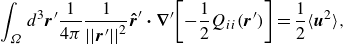 \begin{align} \int _{\Omega }d^{3}\boldsymbol{r}^{\prime }\frac {1}{4\pi } \frac {1}{{\left ||\boldsymbol{r}^{\prime }\right |\!|}^{2}}\boldsymbol{\hat r}^{\prime }\boldsymbol{\cdot }\boldsymbol{\nabla }^{\prime } {\left [ -\frac {1}{2}Q_{ii}(\boldsymbol{r}^{\prime }) \right ]} &= \frac {1}{2}\langle {\boldsymbol{u}^{2}}\rangle , \end{align}
where we have used
 $Q_{ii}(\boldsymbol{0})/2 = \langle {\boldsymbol{u}^{2}} \rangle /2$
and
$Q_{ii}(\boldsymbol{0})/2 = \langle {\boldsymbol{u}^{2}} \rangle /2$
and
 $\boldsymbol{\hat r}^{\prime } := \boldsymbol{r}^{\prime }/{ \|\boldsymbol{r}^{\prime } \|}$
. From (3.6), we can define a three-dimensional spatial energy-density function
$\boldsymbol{\hat r}^{\prime } := \boldsymbol{r}^{\prime }/{ \|\boldsymbol{r}^{\prime } \|}$
. From (3.6), we can define a three-dimensional spatial energy-density function
 \begin{align} V\!(\boldsymbol{r})&:=\frac {1}{4\pi } \frac {1}{\|\boldsymbol{r}\|^{2}}\boldsymbol{\hat r}\boldsymbol{\cdot }\boldsymbol{\nabla } {\left [ -\frac {1}{2}Q_{ii}(\boldsymbol{r}) \right ]} = \frac {1}{4\pi \|\boldsymbol{r}\|^{2}}D_{\boldsymbol{r}}{\left [ -\frac {1}{2}Q_{ii}(\boldsymbol{r}) \right ]}, \end{align}
where
 $D_{\boldsymbol{r}}:=\boldsymbol{\hat r}\boldsymbol{\cdot }\boldsymbol{\nabla }$
is the directional derivative. For the case of homogeneous isotropic turbulence, we can simplify (3.7) by averaging
$D_{\boldsymbol{r}}:=\boldsymbol{\hat r}\boldsymbol{\cdot }\boldsymbol{\nabla }$
is the directional derivative. For the case of homogeneous isotropic turbulence, we can simplify (3.7) by averaging
 $V\!(\boldsymbol{r})$
over a spherical shell
$V\!(\boldsymbol{r})$
over a spherical shell
 $S(r)$
,
$S(r)$
,
![]() , similar to the definition of
, similar to the definition of
 $E(k)$
(cf. (1.2)). This transforms (3.7) to (2.4), thereby verifying self-consistency of the derivation discussed here.
$E(k)$
(cf. (1.2)). This transforms (3.7) to (2.4), thereby verifying self-consistency of the derivation discussed here.
Can the above analysis be readily generalised for inhomogeneous turbulence? For example, we may expect that (3.7) simply generalises to (cf. (18) in Hamba Reference Hamba2015)
 \begin{align} V\!(\boldsymbol{x}, \boldsymbol{r})&:= \frac {1}{4\pi \|\boldsymbol{r}\|^{2}}D_{\boldsymbol{r}}{\left [ -\frac {1}{2}Q_{ii}(\boldsymbol{x}, \boldsymbol{r}) \right ]}. \end{align}
We urge caution with this step. As we noted in the discussion of (3.4), the surface integral vanishes for homogeneous turbulence. But that may not hold for inhomogeneous turbulence. Note, however, that for the case of inhomogeneous turbulence where there exists one or more directions of homogeneity (e.g. streamwise and azimuthal directions in a fully developed pipe flow), the surface integral still vanishes when
 $\boldsymbol{r}$
is restricted to the homogeneous directions.
$\boldsymbol{r}$
is restricted to the homogeneous directions.
4. One-dimensional spatial energy-density functions
In the analysis so far, we considered the three-dimensional spatial energy-density function. Here, we turn attention to the corresponding one-dimensional functions. In the spectral space, one-dimensional spectral energy-density functions, typically denoted by
 $E_{11}(k_1), E_{22}(k_1),\dots$
, are well known (Davidson Reference Davidson2004). They are particularly useful in the analysis of experimental data, wherein measuring the (three-dimensional)
$E_{11}(k_1), E_{22}(k_1),\dots$
, are well known (Davidson Reference Davidson2004). They are particularly useful in the analysis of experimental data, wherein measuring the (three-dimensional)
 $E(k)$
is very challenging. In the same spirit, here we seek to derive one-dimensional spatial energy-density functions.
$E(k)$
is very challenging. In the same spirit, here we seek to derive one-dimensional spatial energy-density functions.
For a homogeneous anisotropic turbulent flow, consider the direction
 $\boldsymbol{r}=r_{1}\boldsymbol{\hat e}_{1}$
. The associated longitudinal velocity correlation function can be expressed as (cf. (3.1))
$\boldsymbol{r}=r_{1}\boldsymbol{\hat e}_{1}$
. The associated longitudinal velocity correlation function can be expressed as (cf. (3.1))
 \begin{align} \frac {1}{2}Q_{11}(r_{1}\boldsymbol{\hat e}_{1}) &=\int _{0}^{\infty }{\textrm d}\xi {\left [ \frac {1}{2}Q_{11}(\xi \boldsymbol{\hat e}_{1}) \right ]} \delta (\xi -r_{1}). \end{align}
Following the analysis of § 2, we can simplify the above integral as
 \begin{align} \frac {1}{2}Q_{11}(r_{1}\boldsymbol{\hat e}_{1}) &=\int _{r_{1}}^{\infty }{\textrm d}\xi \frac {\partial }{\partial \xi }{\left [ -\frac {1}{2}Q_{11}(\xi \boldsymbol{\hat e}_{1}) \right ]}, \end{align}
where we have used
 $Q_{11}(r_{1}\to \infty ) = 0$
. Taking the limit
$Q_{11}(r_{1}\to \infty ) = 0$
. Taking the limit
 $r_{1}\to 0$
leads to an energy constraint
$r_{1}\to 0$
leads to an energy constraint
 \begin{align} \int _{0}^{\infty }{\textrm d}\xi {\left [ -\frac {\partial }{\partial \xi } \frac {1}{2}Q_{11}(\xi \boldsymbol{\hat e}_{1}) \right ]} &= \frac {1}{2}\langle {u_{1}^{2}} \rangle , \end{align}
where we have used
 $Q_{11}(\boldsymbol{0})/2 = \langle {u_{1}^{2}} \rangle /2$
. We can now define a (one-dimensional) longitudinal spatial energy-density function
$Q_{11}(\boldsymbol{0})/2 = \langle {u_{1}^{2}} \rangle /2$
. We can now define a (one-dimensional) longitudinal spatial energy-density function
 \begin{align} V_{11}(r_{1})&:= -\frac {\partial }{\partial r_{1}}\frac {1}{2}Q_{11}(r_{1}\boldsymbol{\hat e}_{1}), \end{align}
where
 $V_{11}(r_{1}){\textrm d}r_{1}$
is the contribution to the turbulent energy component
$V_{11}(r_{1}){\textrm d}r_{1}$
is the contribution to the turbulent energy component
 $({1}/{2})\langle {u_{1}^{2}} \rangle$
from eddies of size in the range
$({1}/{2})\langle {u_{1}^{2}} \rangle$
from eddies of size in the range
 $(r_{1},r_{1}+{\textrm d}r_{1})$
.
$(r_{1},r_{1}+{\textrm d}r_{1})$
.
Following the above procedure, we can define (one-dimensional) transverse spatial energy-density functions
 \begin{align} V_{22}(r_{1})&:= -\frac {\partial }{\partial r_{1}}\frac {1}{2}Q_{22}(r_{1}\boldsymbol{\hat e}_{1}), \end{align}
 \begin{align} V_{33}(r_{1})&:= -\frac {\partial }{\partial r_{1}}\frac {1}{2}Q_{33}(r_{1}\boldsymbol{\hat e}_{1}). \end{align}
These functions satisfy the corresponding energy constraints
 \begin{align} \int _{0}^{\infty }{\textrm d}r_{1} V_{22}(r_{1})&= \frac {1}{2}\langle {u_{2}^{2}} \rangle , \end{align}
 \begin{align} \int _{0}^{\infty }{\textrm d}r_{1} V_{33}(r_{1})&= \frac {1}{2}\langle {u_{3}^{2}} \rangle . \end{align}
(In Appendix C, we discuss the relationship between the spectral and spatial variants of the one-dimensional energy-density functions.) Also note that the analysis discussed here can be easily extended to other directions, namely,
 $\boldsymbol{r}=r_{2}\boldsymbol{\hat e}_{2}$
and
$\boldsymbol{r}=r_{2}\boldsymbol{\hat e}_{2}$
and
 $\boldsymbol{r}=r_{3}\boldsymbol{\hat e}_{3}$
. This yields one-dimensional spatial energy-density functions such as
$\boldsymbol{r}=r_{3}\boldsymbol{\hat e}_{3}$
. This yields one-dimensional spatial energy-density functions such as
 $V_{11}(r_{2}), V_{11}(r_{3})$
, etc.
$V_{11}(r_{2}), V_{11}(r_{3})$
, etc.
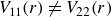
Last, we consider homogeneous isotropic turbulence. In this case, (4.4) and (4.5) transform to
 \begin{align} V_{11}(r)&:= -\frac {\partial }{\partial r}\frac {1}{2}Q_{11}(r)=-\frac {u^{2}}{2}\frac {\partial }{\partial r}f(r), \end{align}
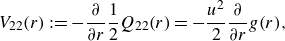 \begin{align} V_{22}(r)&:= -\frac {\partial }{\partial r}\frac {1}{2}Q_{22}(r) =-\frac {u^{2}}{2}\frac {\partial }{\partial r}g(r), \end{align}
 \begin{align} V_{33}(r)&\;= V_{22}(r), \end{align}
where
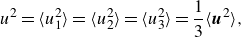 \begin{align} u^{2}&=\langle {u_{1}^{2}} \rangle =\langle {u_{2}^{2}} \rangle =\langle {u_{3}^{2}} \rangle =\frac {1}{3}\langle {\boldsymbol{u}^{2}} \rangle , \end{align}
and
 $f(r):=Q_{11}(r)/u^2$
and
$f(r):=Q_{11}(r)/u^2$
and
 $g(r):=Q_{22}(r)/u^2$
are the longitudinal and transverse velocity correlation functions, respectively.
$g(r):=Q_{22}(r)/u^2$
are the longitudinal and transverse velocity correlation functions, respectively.
Notably, our proposal for
 $V_{11}(r)$
(4.7a
) can be related with a previous result. The kinematic relationship
$V_{11}(r)$
(4.7a
) can be related with a previous result. The kinematic relationship
 \begin{align} \langle {{\left [ \Delta \upsilon (r) \right ]}^{2}} \rangle &=2u^{2}{[ 1-f(r) ]}, \end{align}
can be rewritten as
 \begin{align} \frac {1}{4}\frac {\partial }{\partial r}\langle {{\left [ \Delta \upsilon (r) \right ]}^{2}} \rangle =-\frac {u^{2}}{2}\frac {\partial f}{\partial r}, \end{align}
which, when substituted into (4.7a ), leads to
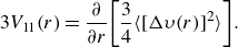 \begin{align} 3 V_{11}(r)=\frac {\partial }{\partial r}{\left [ \frac {3}{4}\langle {{[ }\Delta \upsilon (r)]^{2}} \rangle \right ]}. \end{align}
Note that this is the Townsend–Davidson function,
 $V_{\textit{TD}}(r)$
(1.6). Now, because
$V_{\textit{TD}}(r)$
(1.6). Now, because
 $V_{11}(r) \neq V_{22}(r)$
, it follows that
$V_{11}(r) \neq V_{22}(r)$
, it follows that
 $V_{\textit{TD}}(r) = 3 V_{11}(r) \neq V\!(r)$
(where we have used (B1c
)). We can now see why, starting from Townsend’s proposal, Davidson (Reference Davidson2004) and Hamba (Reference Hamba2015) arrived at disparate forms of energy-density functions.
$V_{\textit{TD}}(r) = 3 V_{11}(r) \neq V\!(r)$
(where we have used (B1c
)). We can now see why, starting from Townsend’s proposal, Davidson (Reference Davidson2004) and Hamba (Reference Hamba2015) arrived at disparate forms of energy-density functions.
5. Characteristic properties of spatial energy-density functions
In § 1, we listed three characteristic properties for a spatial energy-density function. Here, we consider each property in turn. For simplicity, we focus on homogeneous isotropic turbulence.
Interestingly, property (i) that a density function should be non-negative turns out to be the most difficult to satisfy. Indeed, to our knowledge, none of the functional forms proposed to date are guaranteed to be non-negative. The same is true for
 $V\!(r)$
,
$V\!(r)$
,
 $V_{11}(r)$
and
$V_{11}(r)$
and
 $V_{22}(r)$
. The reason can be understood by expressing these functions in terms of
$V_{22}(r)$
. The reason can be understood by expressing these functions in terms of
 $E(k)$
. Starting with the relationship
$E(k)$
. Starting with the relationship
 \begin{align} -\frac {1}{2} u^2 f(r)&=\int _{0}^{\infty }{\textrm d}kE(k)G_{1}(kr),\quad G_{1}(x)=\frac {x\cos x - \sin x}{x^{3}}, \end{align}
and using (4.11), (B1a ), and (B1b ), we can write
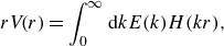 \begin{align} rV\!(r)&=\int _{0}^{\infty }{\textrm d}kE(k)H(kr), \end{align}
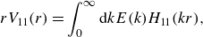 \begin{align} rV_{11}(r)&=\int _{0}^{\infty }{\textrm d}kE(k)H_{11}(kr), \end{align}
 \begin{align} rV_{22}(r)&=\int _{0}^{\infty }{\textrm d}kE(k)H_{22}(kr), \end{align}
where
 \begin{align} \begin{aligned} H(kr)&=\frac {1}{r^{3}}\frac {\partial }{\partial r}{[ r^{4}H_{11}(kr) ]},\\ H_{11}(kr)&=r\frac {\partial }{\partial r}G_{1}(kr),\\ H_{22}(kr)&=\frac {1}{2r^2}\frac {\partial }{\partial r}{[ r^{3}H_{11}(kr) ]}. \end{aligned} \end{align}
Now, since the kernels
 $H(x)$
,
$H(x)$
,
 $H_{11}(x)$
and
$H_{11}(x)$
and
 $H_{22}(x)$
all oscillate about the
$H_{22}(x)$
all oscillate about the
 $x$
-axis taking positive and negative values (figure 1),
$x$
-axis taking positive and negative values (figure 1),
 $V\!(r)$
,
$V\!(r)$
,
 $V_{11}(r)$
and
$V_{11}(r)$
and
 $V_{22}(r)$
are not guaranteed to be non-negative. Thus, strictly speaking, these functions are not density functions; Davidson (Reference Davidson2004) suggested using the term ‘signature function’ instead. For simplicity, we shall refer to them as density functions.
$V_{22}(r)$
are not guaranteed to be non-negative. Thus, strictly speaking, these functions are not density functions; Davidson (Reference Davidson2004) suggested using the term ‘signature function’ instead. For simplicity, we shall refer to them as density functions.
Shapes of the kernels
 $H(x)$
,
$H(x)$
,
 $H_{11}(x)$
and
$H_{11}(x)$
and
 $H_{22}(x)$
.
$H_{22}(x)$
.
Property (ii) expresses an energy constraint. Because we have derived
 $V\!(r)$
and its one-dimensional variants by imposing this constraint (cf. § 2), these functions satisfy the constraint by construction.
$V\!(r)$
and its one-dimensional variants by imposing this constraint (cf. § 2), these functions satisfy the constraint by construction.
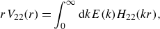
For checking property (iii), consider a random distribution of Townsend’s model eddies of a fixed size
 $\ell _{e}$
in a two-dimensional plane (Townsend Reference Townsend1976). For this turbulent flow, we can write
$\ell _{e}$
in a two-dimensional plane (Townsend Reference Townsend1976). For this turbulent flow, we can write
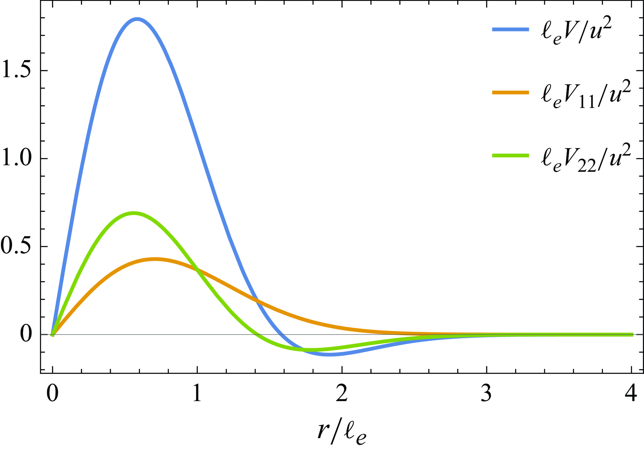
 $f(r)=\exp (-r^{2}/\ell _{e}^{2})$
. From (2.4) and (4.7), it follows that
$f(r)=\exp (-r^{2}/\ell _{e}^{2})$
. From (2.4) and (4.7), it follows that
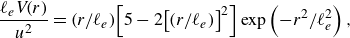 \begin{align} \frac {\ell _e V\!(r)}{u^{2}}&={ (r/\ell _{e}) }{\left [ 5-2{\left [ (r/\ell _{e}) \right ]}^{2} \right ]}\exp \left(-r^{2}/\ell _{e}^{2}\right), \end{align}
 \begin{align} \frac {\ell _e V_{11}(r)}{u^{2}}&={(r/\ell _{e}) }\exp \left(-r^{2}/\ell _{e}^{2}\right), \end{align}
 \begin{align} \frac {\ell _e V_{22}(r)}{u^{2}}&={ (r/\ell _{e})}{\left [ 2-{\left [ (r/\ell _{e}) \right ]}^{2} \right ]}\exp \left(-r^{2}/\ell _{e}^{2}\right). \end{align}
In figure 2, we plot the energy distribution across eddy sizes from (5.4). In all cases, there is a clear peak around
 $r \sim \ell _{e}$
. Notably, in this idealised flow, only
$r \sim \ell _{e}$
. Notably, in this idealised flow, only
 $V_{11}(r)$
is non-negative for all
$V_{11}(r)$
is non-negative for all
 $r$
.
$r$
.
Distribution of energy across eddy sizes as quantified by
 $\ell _e V\!(r)/u^2$
,
$\ell _e V\!(r)/u^2$
,
 $\ell _e V_{11}(r)/u^2$
and
$\ell _e V_{11}(r)/u^2$
and
 $\ell _e V_{22}(r)/u^2$
for a random distribution of Townsend’s model eddies of fixed size
$\ell _e V_{22}(r)/u^2$
for a random distribution of Townsend’s model eddies of fixed size
 $\ell _{e}$
.
$\ell _{e}$
.
The above discussion of property (iii) points to a crucial advantage of one-dimensional spatial energy-density functions over their spectral counterparts. In the spectral space, this property reads: for a random distribution of eddies of fixed size
 $\ell _{e}$
, the corresponding
$\ell _{e}$
, the corresponding
 $E(k)$
(or any of its one-dimensional variants) manifests a clear peak around
$E(k)$
(or any of its one-dimensional variants) manifests a clear peak around
 $k \sim \ell _{e}^{-1}$
(Davidson Reference Davidson2004). While
$k \sim \ell _{e}^{-1}$
(Davidson Reference Davidson2004). While
 $E(k)$
satisfies this property,
$E(k)$
satisfies this property,
 $E_{11}(k)$
and
$E_{11}(k)$
and
 $E_{22}(k)$
do not. Instead of having a peak around
$E_{22}(k)$
do not. Instead of having a peak around
 $k \sim \ell _{e}^{-1}$
, they attain their maxima at
$k \sim \ell _{e}^{-1}$
, they attain their maxima at
 $k = 0$
. (This is due to the phenomenon of aliasing (Davidson Reference Davidson2004).) As a result, it is difficult to interpret
$k = 0$
. (This is due to the phenomenon of aliasing (Davidson Reference Davidson2004).) As a result, it is difficult to interpret
 $E_{11}(k)$
and
$E_{11}(k)$
and
 $E_{22}(k)$
in terms of eddy sizes, even though they satisfy the energy constraint. By contrast, as we have seen,
$E_{22}(k)$
in terms of eddy sizes, even though they satisfy the energy constraint. By contrast, as we have seen,
 $V_{11}(r)$
and
$V_{11}(r)$
and
 $V_{22}(r)$
manifest a clear peak around
$V_{22}(r)$
manifest a clear peak around
 $r \sim \ell _{e}$
(figure 2), underscoring their clear advantage over
$r \sim \ell _{e}$
(figure 2), underscoring their clear advantage over
 $E_{11}(k)$
and
$E_{11}(k)$
and
 $E_{22}(k)$
.
$E_{22}(k)$
.
6. Analysis of empirical data
In § 4, we noted that one-dimensional spatial energy-density functions can be useful for analysis of empirical data. Here, for illustration, we analyse data from two canonical wall-bounded flows: channel flow and pipe flow. We take
 $\boldsymbol{\hat e}_1$
along the streamwise direction,
$\boldsymbol{\hat e}_1$
along the streamwise direction,
 $\boldsymbol{\hat e}_2$
along the wall-normal direction and
$\boldsymbol{\hat e}_2$
along the wall-normal direction and
 $\boldsymbol{\hat e}_3$
along the spanwise direction (for channel flow) or the azimuthal direction (for pipe flow). The origin of the coordinate system is at the wall (for channel flow) and the centreline (for pipe flow). Similar to most studies of empirical data, we focus on the case where the position
$\boldsymbol{\hat e}_3$
along the spanwise direction (for channel flow) or the azimuthal direction (for pipe flow). The origin of the coordinate system is at the wall (for channel flow) and the centreline (for pipe flow). Similar to most studies of empirical data, we focus on the case where the position
 $x_2$
is fixed and
$x_2$
is fixed and
 $\boldsymbol{r}$
is oriented along
$\boldsymbol{r}$
is oriented along
 $\boldsymbol{\hat e}_1$
. Note that the flow is homogeneous along
$\boldsymbol{\hat e}_1$
. Note that the flow is homogeneous along
 $\boldsymbol{\hat e}_1$
(and
$\boldsymbol{\hat e}_1$
(and
 $\boldsymbol{\hat e}_3$
), but not along
$\boldsymbol{\hat e}_3$
), but not along
 $\boldsymbol{\hat e}_2$
.
$\boldsymbol{\hat e}_2$
.
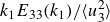
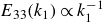
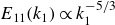
First, we consider the scaling
 $E_{11}(k_1) \propto k_1^{-1}$
(Perry, Henbest & Chong Reference Perry, Henbest and Chong1986). In the past decades, this scaling has attracted considerable attention and no small measure of debate (see, e.g. Smits, McKeon & Marusic (Reference Smits, McKeon and Marusic2011), Appendix A in Zamalloa et al. (Reference Zamalloa, Ng, Chakraborty and Gioia2014)). The scaling appears over a limited spatial region and at high Reynolds numbers, Re; curiously, however, it disappears at even higher Re (Rosenberg et al. Reference Rosenberg, Hultmark, Vallikivi, Bailey and Smits2013; Yamamoto & Tsuji Reference Yamamoto and Tsuji2018). The range of
$E_{11}(k_1) \propto k_1^{-1}$
(Perry, Henbest & Chong Reference Perry, Henbest and Chong1986). In the past decades, this scaling has attracted considerable attention and no small measure of debate (see, e.g. Smits, McKeon & Marusic (Reference Smits, McKeon and Marusic2011), Appendix A in Zamalloa et al. (Reference Zamalloa, Ng, Chakraborty and Gioia2014)). The scaling appears over a limited spatial region and at high Reynolds numbers, Re; curiously, however, it disappears at even higher Re (Rosenberg et al. Reference Rosenberg, Hultmark, Vallikivi, Bailey and Smits2013; Yamamoto & Tsuji Reference Yamamoto and Tsuji2018). The range of
 $k_1$
for this scaling corresponds to the large eddies. In this regime, using Taylor’s frozen-turbulence hypothesis may incur substantial errors. This limits the use of experimental data since most experiments obtain
$k_1$
for this scaling corresponds to the large eddies. In this regime, using Taylor’s frozen-turbulence hypothesis may incur substantial errors. This limits the use of experimental data since most experiments obtain
 $E_{11}(k_1)$
using Taylor’s hypothesis.
$E_{11}(k_1)$
using Taylor’s hypothesis.
We analyse data from a direct numerical simulation (DNS) of channel flow at friction Reynolds number
 $Re _\tau \approx 5200$
(Lee & Moser Reference Lee and Moser2015) (
$Re _\tau \approx 5200$
(Lee & Moser Reference Lee and Moser2015) (
 $ Re _\tau := u_\tau \delta /\nu$
, where
$ Re _\tau := u_\tau \delta /\nu$
, where
 $u_\tau$
is the friction velocity,
$u_\tau$
is the friction velocity,
 $\delta$
the channel half-width and
$\delta$
the channel half-width and
 $\nu$
the kinematic viscosity). Lee & Moser (Reference Lee and Moser2015) noted that, over a small span of wall-normal distances (
$\nu$
the kinematic viscosity). Lee & Moser (Reference Lee and Moser2015) noted that, over a small span of wall-normal distances (
 $90 \leqslant x_2^+ \leqslant 169$
, where
$90 \leqslant x_2^+ \leqslant 169$
, where
 $x_2^+ := x_2 u_\tau /\nu$
), the premultiplied spectrum
$x_2^+ := x_2 u_\tau /\nu$
), the premultiplied spectrum
 $k_1 E_{11}(k_1)$
manifests a plateau, signalling
$k_1 E_{11}(k_1)$
manifests a plateau, signalling
 $E_{11}(k_1) \propto k_1^{-1}$
(figure 3
a). (Note that Taylor’s hypothesis was not invoked to compute
$E_{11}(k_1) \propto k_1^{-1}$
(figure 3
a). (Note that Taylor’s hypothesis was not invoked to compute
 $E_{11}(k_1)$
.) Expressed in the form of
$E_{11}(k_1)$
.) Expressed in the form of
 $V_{11}(r_1)$
,
$V_{11}(r_1)$
,
 $E_{11}(k_1) \propto k_1^{-1}$
scaling transforms to
$E_{11}(k_1) \propto k_1^{-1}$
scaling transforms to
 $V_{11}(r_1) \propto r_1^{-1}$
. (This transformation follows from dimensional considerations: dimensionally,
$V_{11}(r_1) \propto r_1^{-1}$
. (This transformation follows from dimensional considerations: dimensionally,
 $[k_1 E_{11}(k_1)] = [r_1 V_{11}(r_1)]$
, and thus,
$[k_1 E_{11}(k_1)] = [r_1 V_{11}(r_1)]$
, and thus,
 $E_{11}(k_1) \propto k_1^{-1}$
implies
$E_{11}(k_1) \propto k_1^{-1}$
implies
 $V_{11}(r_1) \propto r_1^{-1}$
.) In figure 3(b), we plot profiles of
$V_{11}(r_1) \propto r_1^{-1}$
.) In figure 3(b), we plot profiles of
 $r_1 V_{11}(r_1)$
corresponding to the spectra of figure 3(a). (We compute
$r_1 V_{11}(r_1)$
corresponding to the spectra of figure 3(a). (We compute
 $V_{11}(r_1)$
from
$V_{11}(r_1)$
from
 $E_{11}(k_1)$
using (C3a).) Unlike
$E_{11}(k_1)$
using (C3a).) Unlike
 $k_1 E_{11}(k_1)$
,
$k_1 E_{11}(k_1)$
,
 $r_1 V_{11}(r_1)$
does not manifest a plateau for most of the spatial region except near
$r_1 V_{11}(r_1)$
does not manifest a plateau for most of the spatial region except near
 $x_2^+ = 169$
. By probing farther from the wall, we find a curious result. For
$x_2^+ = 169$
. By probing farther from the wall, we find a curious result. For
 $169 \leqslant x_2^+ \leqslant 191$
,
$169 \leqslant x_2^+ \leqslant 191$
,
 $k_1 E_{11}(k_1)$
does not manifest a plateau but
$k_1 E_{11}(k_1)$
does not manifest a plateau but
 $r_1 V_{11}(r_1)$
does so (figure 4). Thus,
$r_1 V_{11}(r_1)$
does so (figure 4). Thus,
 $V_{11}(r_1) \propto r_1^{-1}$
scaling prevails over a region that is spatially contiguous to albeit shifted from the
$V_{11}(r_1) \propto r_1^{-1}$
scaling prevails over a region that is spatially contiguous to albeit shifted from the
 $E_{11}(k_1) \propto k_1^{-1}$
scaling region. The results suggest that the spatial domain of the scaling region depends on the diagnostic function employed to evince the scaling.
$E_{11}(k_1) \propto k_1^{-1}$
scaling region. The results suggest that the spatial domain of the scaling region depends on the diagnostic function employed to evince the scaling.
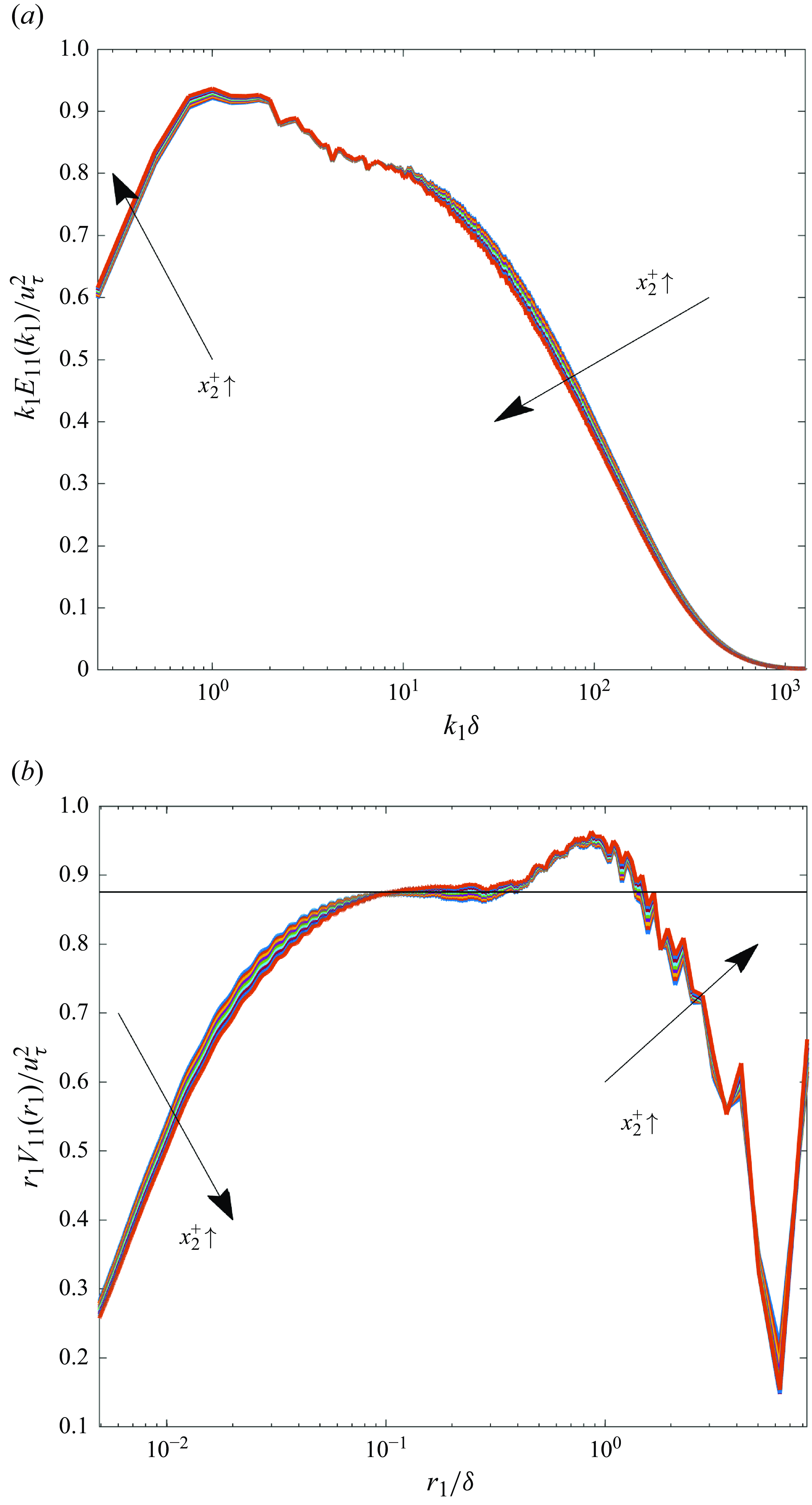
Testing the
 $k_1^{-1}$
and
$k_1^{-1}$
and
 $r_1^{-1}$
scalings for DNS of channel flow at
$r_1^{-1}$
scalings for DNS of channel flow at
 $Re _\tau \approx 5200$
(Lee & Moser Reference Lee and Moser2015): (a) normalised premultiplied spectrum
$Re _\tau \approx 5200$
(Lee & Moser Reference Lee and Moser2015): (a) normalised premultiplied spectrum
 $k_{1} E_{11}(k_{1})/u_{\tau }^{2}$
and (b) normalised premultiplied spatial energy-density function
$k_{1} E_{11}(k_{1})/u_{\tau }^{2}$
and (b) normalised premultiplied spatial energy-density function
 $r_{1}V_{11}(r_{1})/u_{\tau }^{2}$
. Each curve corresponds to a fixed value of
$r_{1}V_{11}(r_{1})/u_{\tau }^{2}$
. Each curve corresponds to a fixed value of
 $x_2^+$
in the range
$x_2^+$
in the range
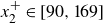 $x_2^+ \in [90, 169]$
.
$x_2^+ \in [90, 169]$
.
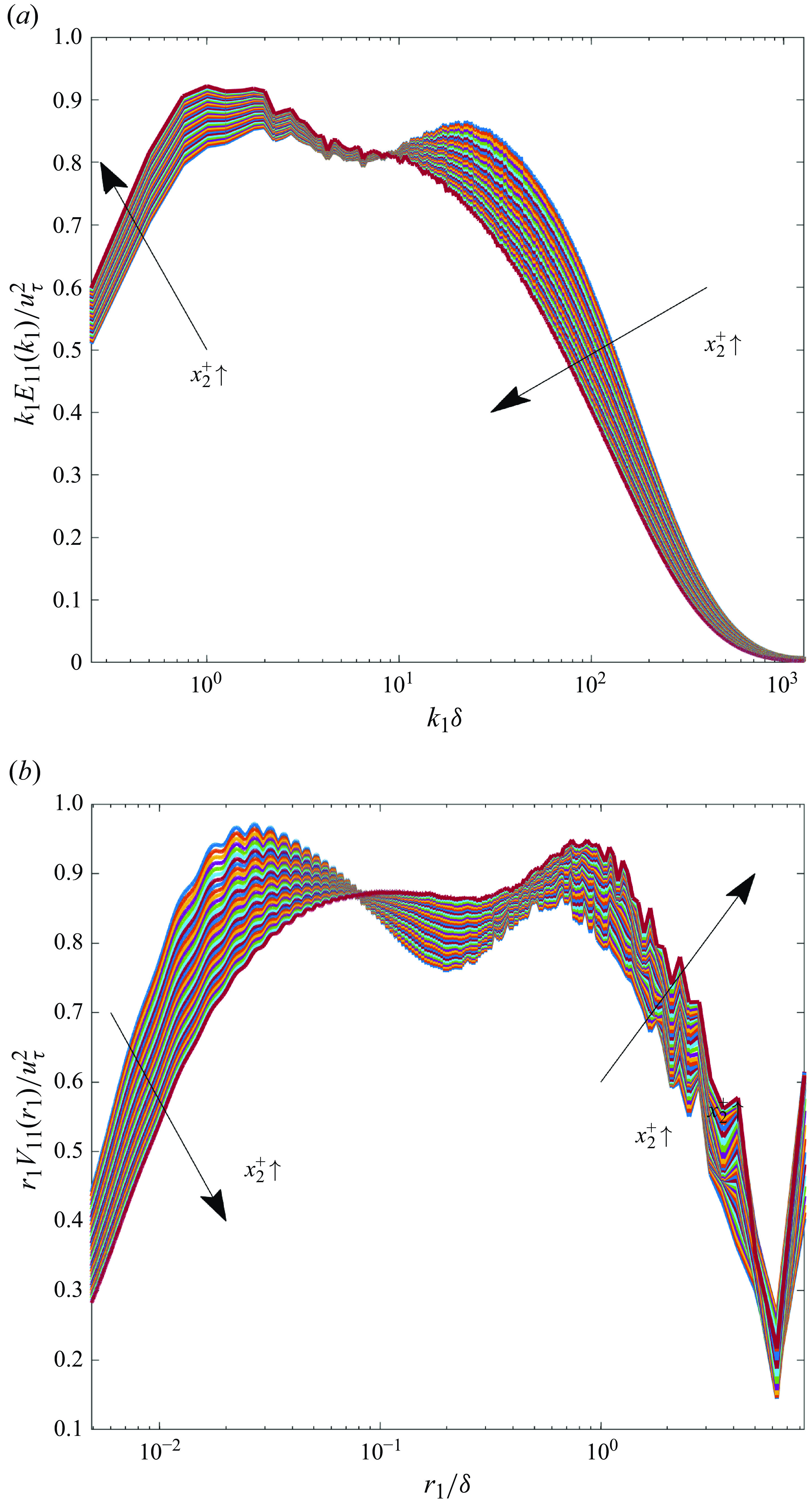
Testing the
 $k_1^{-1}$
and
$k_1^{-1}$
and
 $r_1^{-1}$
scalings for DNS of channel flow at
$r_1^{-1}$
scalings for DNS of channel flow at
 $Re_\tau \approx 5200$
(Lee & Moser Reference Lee and Moser2015): (a) normalised premultiplied spectrum
$Re_\tau \approx 5200$
(Lee & Moser Reference Lee and Moser2015): (a) normalised premultiplied spectrum
 $k_{1} E_{11}(k_{1})/u_{\tau }^{2}$
and (b) normalised premultiplied spatial energy-density function
$k_{1} E_{11}(k_{1})/u_{\tau }^{2}$
and (b) normalised premultiplied spatial energy-density function
 $r_{1}V_{11}(r_{1})/u_{\tau }^{2}$
. Each curve corresponds to a fixed value of
$r_{1}V_{11}(r_{1})/u_{\tau }^{2}$
. Each curve corresponds to a fixed value of
 $x_2^+$
in the range
$x_2^+$
in the range
 $x_2^+ \in [169, 191]$
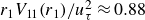
. In the nominal
$x_2^+ \in [169, 191]$
. In the nominal
 $r_1^{-1}$
scaling regime,
$r_1^{-1}$
scaling regime,
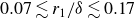
 $0.1\lesssim r_1/\delta \lesssim 0.3$
, the plateau value
$0.1\lesssim r_1/\delta \lesssim 0.3$
, the plateau value
 $r_{1}V_{11}(r_{1})/u_{\tau }^{2} \approx 0.88$
(black line, panel b).
$r_{1}V_{11}(r_{1})/u_{\tau }^{2} \approx 0.88$
(black line, panel b).
In figure 3(a), we note the bimodal structure of
 $k_1 E_{11}(k_1)$
, wherein the
$k_1 E_{11}(k_1)$
, wherein the
 $k_1^{-1}$
scaling regime is flanked on its sides by two local peaks. These peaks are considered to be signatures of organised motions at large scales, the left peak corresponding to ‘very-large-scale motions’ (VLSMs) and the right peak to ‘large-scale motions’ (LSMs) (Kim & Adrian Reference Kim and Adrian1999). We represent these peaks as
$k_1^{-1}$
scaling regime is flanked on its sides by two local peaks. These peaks are considered to be signatures of organised motions at large scales, the left peak corresponding to ‘very-large-scale motions’ (VLSMs) and the right peak to ‘large-scale motions’ (LSMs) (Kim & Adrian Reference Kim and Adrian1999). We represent these peaks as
 $k_1^{\textit{VLSM}}$
and
$k_1^{\textit{VLSM}}$
and
 $k_1^{\textit{LSM}}$
, respectively. The attendant eddy sizes are estimated as
$k_1^{\textit{LSM}}$
, respectively. The attendant eddy sizes are estimated as
 $\ell _{{VLSM}} = 2\pi /k_1^{\textit{VLSM}}$
and
$\ell _{{VLSM}} = 2\pi /k_1^{\textit{VLSM}}$
and
 $\ell _{{LSM}} = 2\pi /k_1^{\textit{LSM}}$
, respectively. From figure 3(a), we find
$\ell _{{LSM}} = 2\pi /k_1^{\textit{LSM}}$
, respectively. From figure 3(a), we find
 $\ell _{{VLSM}} \approx 6 \delta$
and
$\ell _{{VLSM}} \approx 6 \delta$
and
 $\ell _{{LSM}} \approx 0.3 \delta$
. That organised motions exist at scales
$\ell _{{LSM}} \approx 0.3 \delta$
. That organised motions exist at scales
 $\gtrsim \!\delta$
, as is the case with VLSMs, is a surprising finding and an active area of inquiry (Smits et al. Reference Smits, McKeon and Marusic2011).
$\gtrsim \!\delta$
, as is the case with VLSMs, is a surprising finding and an active area of inquiry (Smits et al. Reference Smits, McKeon and Marusic2011).
We wish to draw attention to some potential problems in inferring the eddy sizes using
 $2 \pi /k_1$
. As discussed in § 1, eddies are not waves – consequently, the wavelength of a Fourier mode may not directly correspond to an eddy size. More important, as we have noted in § 5, it is difficult to infer eddy sizes from
$2 \pi /k_1$
. As discussed in § 1, eddies are not waves – consequently, the wavelength of a Fourier mode may not directly correspond to an eddy size. More important, as we have noted in § 5, it is difficult to infer eddy sizes from
 $E_{11}(k_1)$
. Shifting from the Fourier space to the real space may prove useful. Interestingly, similar to its spectral counterpart,
$E_{11}(k_1)$
. Shifting from the Fourier space to the real space may prove useful. Interestingly, similar to its spectral counterpart,
 $r_1 V_{11}(r_1)$
also manifests a bimodal structure (figure 3
b). Analogous to the discussion of the peaks of
$r_1 V_{11}(r_1)$
also manifests a bimodal structure (figure 3
b). Analogous to the discussion of the peaks of
 $k_1 E_{11}(k_1)$
, we can ascribe the left peak to signal LSMs and the right peak to signal VLSMs. The attendant eddy sizes can be estimated as the values of
$k_1 E_{11}(k_1)$
, we can ascribe the left peak to signal LSMs and the right peak to signal VLSMs. The attendant eddy sizes can be estimated as the values of
 $r_1$
corresponding to these peaks. We find
$r_1$
corresponding to these peaks. We find
 $\ell _{{LSM}} \approx 0.03 \delta$
and
$\ell _{{LSM}} \approx 0.03 \delta$
and
 $\ell _{{VLSM}} \approx 0.8 \delta$
. Notably, now the organised motions inhabit scales
$\ell _{{VLSM}} \approx 0.8 \delta$
. Notably, now the organised motions inhabit scales
 $\lesssim \!\delta$
, consistent with the standard conceptual picture of turbulent eddies. We suggest that an extensive study of empirical data on wall-bounded flows along these lines may yield valuable insights into the structure of organised motions at large scales.
$\lesssim \!\delta$
, consistent with the standard conceptual picture of turbulent eddies. We suggest that an extensive study of empirical data on wall-bounded flows along these lines may yield valuable insights into the structure of organised motions at large scales.
Returning to the
 $k_1^{-1}$
and
$k_1^{-1}$
and
 $r_1^{-1}$
scalings, we now turn attention to components other than
$r_1^{-1}$
scalings, we now turn attention to components other than
 $E_{11}(k_1)$
and
$E_{11}(k_1)$
and
 $V_{11}(r_1)$
. Specifically, we consider
$V_{11}(r_1)$
. Specifically, we consider
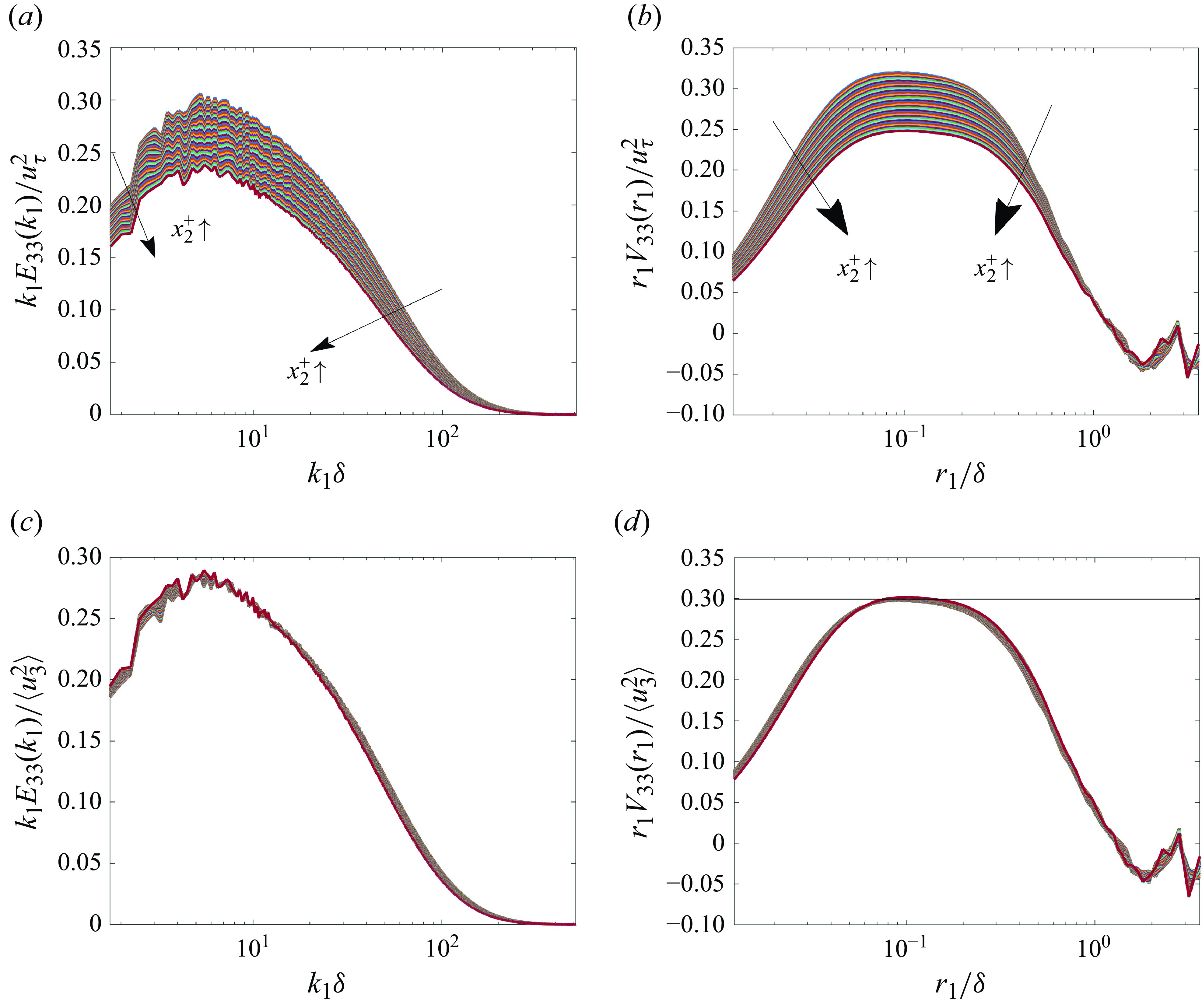
 $E_{33}(k_1)$
and
$E_{33}(k_1)$
and
 $V_{33}(r_1)$
for DNS of channel flow at
$V_{33}(r_1)$
for DNS of channel flow at
 $Re_\tau = 2000$
(Lee & Moser Reference Lee and Moser2015). (We compute
$Re_\tau = 2000$
(Lee & Moser Reference Lee and Moser2015). (We compute
 $V_{33}(r_1)$
from
$V_{33}(r_1)$
from
 $E_{33}(k_1)$
using (C3c
).) Over the span
$E_{33}(k_1)$
using (C3c
).) Over the span
 $902 \leqslant x_2^+ \leqslant 1198$
, it is difficult to discern a plateau in
$902 \leqslant x_2^+ \leqslant 1198$
, it is difficult to discern a plateau in
 $k_1 E_{33}(k_1)$
(figure 5
a). By contrast,
$k_1 E_{33}(k_1)$
(figure 5
a). By contrast,
 $r_1 V_{33}(r_1)$
manifests a plateau, signalling
$r_1 V_{33}(r_1)$
manifests a plateau, signalling
 $V_{33}(r_1) \propto r_1^{-1}$
(figure 5
b). Unlike the case in figure 3(b), the plateau for the curves corresponding to different
$V_{33}(r_1) \propto r_1^{-1}$
(figure 5
b). Unlike the case in figure 3(b), the plateau for the curves corresponding to different
 $x_2^+$
positions do not collapse when normalised as
$x_2^+$
positions do not collapse when normalised as
 $r_{1}V_{33}(r_{1})/u_{\tau }^{2}$
. But, when normalised as
$r_{1}V_{33}(r_{1})/u_{\tau }^{2}$
. But, when normalised as
 $r_{1}V_{33}(r_{1})/\langle {u_{3}^{2}} \rangle$
, they collapse (figure 5
d). (The normalised curves for
$r_{1}V_{33}(r_{1})/\langle {u_{3}^{2}} \rangle$
, they collapse (figure 5
d). (The normalised curves for
 $k_{1} E_{33}(k_{1})/\langle {u_{3}^{2}} \rangle$
also collapse, but unlike its real-space counterpart, there is no plateau; figure 5(c).) Remarkably, the collapse occurs not only in the plateau region, but over the whole range of
$k_{1} E_{33}(k_{1})/\langle {u_{3}^{2}} \rangle$
also collapse, but unlike its real-space counterpart, there is no plateau; figure 5(c).) Remarkably, the collapse occurs not only in the plateau region, but over the whole range of
 $r_1$
. In figure 5(b), we can also see one drawback of
$r_1$
. In figure 5(b), we can also see one drawback of
 $V_{33}(r_1)$
– it becomes negative for
$V_{33}(r_1)$
– it becomes negative for
 $r_1 \gt \delta$
. It does, however, satisfy a weaker condition,
$r_1 \gt \delta$
. It does, however, satisfy a weaker condition,
 $\int _0^{r_1} {\textrm d}r_1 V_{33}(r_1) \geqslant 0$
(Davidson Reference Davidson2004).
$\int _0^{r_1} {\textrm d}r_1 V_{33}(r_1) \geqslant 0$
(Davidson Reference Davidson2004).
Testing the
 $k_1^{-1}$
and
$k_1^{-1}$
and
 $r_1^{-1}$
scalings for DNS of channel flow at Re
$r_1^{-1}$
scalings for DNS of channel flow at Re
 $_\tau$
= 2000 (Lee & Moser Reference Lee and Moser2015): (a) normalised premultiplied spectrum
$_\tau$
= 2000 (Lee & Moser Reference Lee and Moser2015): (a) normalised premultiplied spectrum
 $k_{1} E_{33}(k_{1})/u_{\tau }^{2}$
; (b) normalised premultiplied spatial energy-density function
$k_{1} E_{33}(k_{1})/u_{\tau }^{2}$
; (b) normalised premultiplied spatial energy-density function
 $r_{1}V_{33}(r_{1})/u_{\tau }^{2}$
; (c) normalised premultiplied spectrum
$r_{1}V_{33}(r_{1})/u_{\tau }^{2}$
; (c) normalised premultiplied spectrum
 $k_{1} E_{33}(k_{1})/\langle {u_{3}^{2}} \rangle$
; (d) normalised premultiplied spatial energy-density function
$k_{1} E_{33}(k_{1})/\langle {u_{3}^{2}} \rangle$
; (d) normalised premultiplied spatial energy-density function
 $r_{1}V_{33}(r_{1})/\langle {u_{3}^{2}} \rangle$
. Each curve corresponds to a fixed value of
$r_{1}V_{33}(r_{1})/\langle {u_{3}^{2}} \rangle$
. Each curve corresponds to a fixed value of
 $x_2^+$
in the range
$x_2^+$
in the range
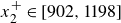 $x_2^+ \in [902, 1198]$
. In the nominal
$x_2^+ \in [902, 1198]$
. In the nominal
 $r_1^{-1}$
scaling regime,
$r_1^{-1}$
scaling regime,
 $0.07\lesssim r_1/\delta \lesssim 0.17$
, the plateau value
$0.07\lesssim r_1/\delta \lesssim 0.17$
, the plateau value
 $r_{1}V_{33}(r_{1})\langle {u_{3}^{2}} \rangle \approx 0.3$
(black line, panel d).
$r_{1}V_{33}(r_{1})\langle {u_{3}^{2}} \rangle \approx 0.3$
(black line, panel d).
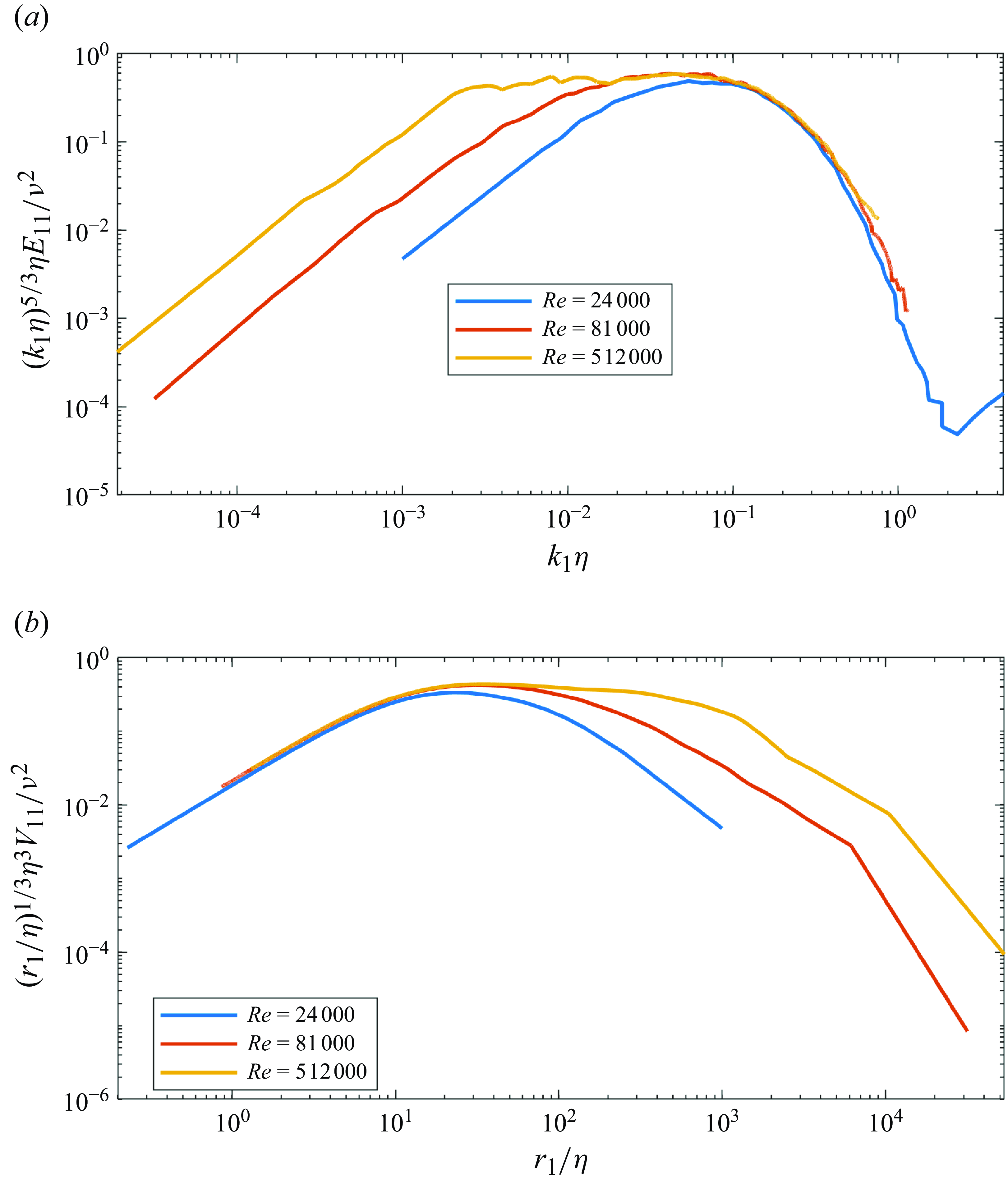
Testing the
 $k_1^{-5/3}$
and
$k_1^{-5/3}$
and
 $r_1^{-1/3}$
scalings at the centreline of a pipe flow from the Princeton superpipe experiment (Bailey et al. Reference Bailey, Hultmark, Schumacher, Yakhot and Smits2009; Rosenberg et al. Reference Rosenberg, Hultmark, Vallikivi, Bailey and Smits2013): (a) normalised premultiplied spectrum
$r_1^{-1/3}$
scalings at the centreline of a pipe flow from the Princeton superpipe experiment (Bailey et al. Reference Bailey, Hultmark, Schumacher, Yakhot and Smits2009; Rosenberg et al. Reference Rosenberg, Hultmark, Vallikivi, Bailey and Smits2013): (a) normalised premultiplied spectrum
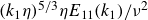 $(k_{1}\eta )^{5/3} \eta E_{11}(k_{1})/\nu ^{2}$
; (b) normalised premultiplied spatial energy-density function
$(k_{1}\eta )^{5/3} \eta E_{11}(k_{1})/\nu ^{2}$
; (b) normalised premultiplied spatial energy-density function
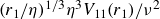 $(r_1/\eta )^{1/3} \eta ^{3} V_{11}(r_{1})/\nu ^{2}$
. The data correspond to
$(r_1/\eta )^{1/3} \eta ^{3} V_{11}(r_{1})/\nu ^{2}$
. The data correspond to
 $Re := U D/\nu = 24\, 000,\, 81\, 000,\, 512\, 000$
, where
$Re := U D/\nu = 24\, 000,\, 81\, 000,\, 512\, 000$
, where
 $U$
is the mean flow velocity and
$U$
is the mean flow velocity and
 $D$
is the pipe diameter.
$D$
is the pipe diameter.
A few additional remarks on the
 $V_{33}(r_1) \propto r_1^{-1}$
scaling may be useful. Because the definition of
$V_{33}(r_1) \propto r_1^{-1}$
scaling may be useful. Because the definition of
 $V_{33}(r_1)$
is a new result, this scaling and the attendant collapse of
$V_{33}(r_1)$
is a new result, this scaling and the attendant collapse of
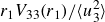 $r_{1}V_{33}(r_{1})/\langle {u_{3}^{2}} \rangle$
are novel findings. It is worth noting that, to our knowledge, the spectral counterpart of this scaling,
$r_{1}V_{33}(r_{1})/\langle {u_{3}^{2}} \rangle$
are novel findings. It is worth noting that, to our knowledge, the spectral counterpart of this scaling,
 $E_{33}(k_1) \propto k_1^{-1}$
, has not been reported, which adds to the novelty of the
$E_{33}(k_1) \propto k_1^{-1}$
, has not been reported, which adds to the novelty of the
 $V_{33}(r_1) \propto r_1^{-1}$
scaling. Further, we observed this scaling for channel flow at
$V_{33}(r_1) \propto r_1^{-1}$
scaling. Further, we observed this scaling for channel flow at
 $Re_\tau = 2000$
but not at
$Re_\tau = 2000$
but not at
 $Re_\tau = 1000$
or
$Re_\tau = 1000$
or
 $Re_\tau \approx 5200$
. It would appear that, similar to the
$Re_\tau \approx 5200$
. It would appear that, similar to the
 $E_{11}(k_1) \propto k_1^{-1}$
scaling, this scaling is also limited to a finite range of
$E_{11}(k_1) \propto k_1^{-1}$
scaling, this scaling is also limited to a finite range of
 $ Re_\tau$
.
$ Re_\tau$
.
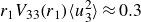
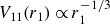
Unlike the
 $k_1^{-1}$
scaling, the classical Kolmogorov inertial-range scaling,
$k_1^{-1}$
scaling, the classical Kolmogorov inertial-range scaling,
 $k^{-5/3}$
, and the related phenomenon of small-scale universality manifest systematic trends with increase of Re (Kolmogorov Reference Kolmogorov1941). To illustrate these trends, we turn to experimental measurements of
$k^{-5/3}$
, and the related phenomenon of small-scale universality manifest systematic trends with increase of Re (Kolmogorov Reference Kolmogorov1941). To illustrate these trends, we turn to experimental measurements of
 $E_{11}(k_1)$
at the centreline of a pipe from the high-Re Princeton superpipe experiment (Bailey et al. Reference Bailey, Hultmark, Schumacher, Yakhot and Smits2009; Rosenberg et al. Reference Rosenberg, Hultmark, Vallikivi, Bailey and Smits2013). In figure 6(a), we plot the premultiplied spectrum
$E_{11}(k_1)$
at the centreline of a pipe from the high-Re Princeton superpipe experiment (Bailey et al. Reference Bailey, Hultmark, Schumacher, Yakhot and Smits2009; Rosenberg et al. Reference Rosenberg, Hultmark, Vallikivi, Bailey and Smits2013). In figure 6(a), we plot the premultiplied spectrum
 $k_1^{5/3} E_{11}(k_1)$
. For
$k_1^{5/3} E_{11}(k_1)$
. For
 $Re \gtrsim 81\,000$
, a plateau emerges, signalling
$Re \gtrsim 81\,000$
, a plateau emerges, signalling
 $E_{11}(k_1) \propto k_1^{-5/3}$
. With increase in Re, the plateau broadens. Moreover, the spectra normalised in Kolmogorov units collapse onto a universal curve at the small scales (at large
$E_{11}(k_1) \propto k_1^{-5/3}$
. With increase in Re, the plateau broadens. Moreover, the spectra normalised in Kolmogorov units collapse onto a universal curve at the small scales (at large
 $k_1 \eta$
, where
$k_1 \eta$
, where
 $\eta$
is the Kolmogorov length scale), signalling small-scale universality. The collapsed region broadens with increase in Re. (This collapse persists even for low-Re transitional pipe flow (Cerbus et al. Reference Cerbus, Liu, Gioia and Chakraborty2020).) The spatial counterpart of the
$\eta$
is the Kolmogorov length scale), signalling small-scale universality. The collapsed region broadens with increase in Re. (This collapse persists even for low-Re transitional pipe flow (Cerbus et al. Reference Cerbus, Liu, Gioia and Chakraborty2020).) The spatial counterpart of the
 $E_{11}(k_1) \propto k_1^{-5/3}$
scaling is
$E_{11}(k_1) \propto k_1^{-5/3}$
scaling is
 $V_{11}(r_1) \propto r_1^{-1/3}$
. (This follows from dimensional considerations: using
$V_{11}(r_1) \propto r_1^{-1/3}$
. (This follows from dimensional considerations: using
 $[k_1 E_{11}(k_1)] = [r_1 V_{11}(r_1)]$
,
$[k_1 E_{11}(k_1)] = [r_1 V_{11}(r_1)]$
,
 $E_{11}(k_1) \propto k_1^{-5/3}$
and
$E_{11}(k_1) \propto k_1^{-5/3}$
and
 $k_1 \propto r_1^{-1}$
, we obtain
$k_1 \propto r_1^{-1}$
, we obtain
 $V_{11}(r_1) \propto r_1^{-1/3}$
.) In figure 6(b), we plot the profiles of
$V_{11}(r_1) \propto r_1^{-1/3}$
.) In figure 6(b), we plot the profiles of
 $r_1^{1/3} V_{11}(r_1)$
corresponding to the spectra of figure 6(a). Complementary to the spectral results, we note a plateau emerging and broadening with increase in Re. Similarly, we note a collapse onto a universal curve at small scales, with the collapsed region broadening with increase in Re.
$r_1^{1/3} V_{11}(r_1)$
corresponding to the spectra of figure 6(a). Complementary to the spectral results, we note a plateau emerging and broadening with increase in Re. Similarly, we note a collapse onto a universal curve at small scales, with the collapsed region broadening with increase in Re.
7. Concluding remarks
Quantifying turbulent kinetic energy distribution in the real space via a spatial energy-density function has been a long-standing quest. Basing our analysis on an energy constraint, in § 2, we derived
 $V\!(r)$
for homogeneous isotropic turbulence. In § 3, we generalised this derivation to anisotropic flows. Our analysis till that point focused on a three-dimensional spatial energy-density function. In § 4, we introduced the concept of one-dimensional spatial energy-density functions.
$V\!(r)$
for homogeneous isotropic turbulence. In § 3, we generalised this derivation to anisotropic flows. Our analysis till that point focused on a three-dimensional spatial energy-density function. In § 4, we introduced the concept of one-dimensional spatial energy-density functions.
Although one-dimensional energy-density functions are well known in the spectral space, that is not the case for the real space. Correspondingly, distinctions between the three-dimensional
 $V\!(r)$
and its one-dimensional variants have not been recognised previously. Indeed, this allowed us to resolve the discrepancies between the Townsend–Davidson function
$V\!(r)$
and its one-dimensional variants have not been recognised previously. Indeed, this allowed us to resolve the discrepancies between the Townsend–Davidson function
 $V_{\textit{TD}}(r)$
and the Townsend–Hamba function
$V_{\textit{TD}}(r)$
and the Townsend–Hamba function
 $V_{\textit{TH}}(r)$
. While both share the same starting point – Townsend’s pioneering proposal of (1.5) – we showed that
$V_{\textit{TH}}(r)$
. While both share the same starting point – Townsend’s pioneering proposal of (1.5) – we showed that
 $V_{\textit{TD}}(r)$
corresponds to
$V_{\textit{TD}}(r)$
corresponds to
 $3 V_{11}(r)$
whereas
$3 V_{11}(r)$
whereas
 $V_{\textit{TH}}(r)$
corresponds to
$V_{\textit{TH}}(r)$
corresponds to
 $V\!(r)$
.
$V\!(r)$
.
A distinctive feature of one-dimensional spatial energy-density functions is that they satisfy the crucial requirement that allows for a one-to-one correspondence with eddy sizes (cf. property (iii) discussed in § 1). Their spectral counterparts, on the other hand, do not satisfy this requirement and thus do not allow for a one-to-one correspondence with eddy sizes. This property makes one-dimensional spatial energy-density functions particularly attractive for the analysis of empirical data. In § 6, we discuss illustrative examples of such analysis. Some of the notable findings from this analysis include: a new spatial region of
 $V_{11}(r_1) \propto r_1^{-1}$
scaling (figure 4); a new scaling regime of
$V_{11}(r_1) \propto r_1^{-1}$
scaling (figure 4); a new scaling regime of
 $V_{33}(r_1) \propto r_1^{-1}$
(figure 5
d); and a potential solution to the puzzlingly large sizes of VLSMs.
$V_{33}(r_1) \propto r_1^{-1}$
(figure 5
d); and a potential solution to the puzzlingly large sizes of VLSMs.
In closing, we wish to draw attention to a critical unfinished task. The fact that in Townsend’s formalism
 $V\!(r)$
,
$V\!(r)$
,
 $V_{11}(r)$
and
$V_{11}(r)$
and
 $V_{22}(r)$
are all not guaranteed to be non-negative is a drawback that is shared by other functions proposed in the literature (Davidson & Pearson Reference Davidson and Pearson2005; Hamba Reference Hamba2015). To our knowledge, no function satisfying the non-negative property has been rigorously developed. As such, there is no proposal that strictly satisfies all three properties necessary for a spatial energy-density function. We submit that finding such a function may yield promising dividends.
$V_{22}(r)$
are all not guaranteed to be non-negative is a drawback that is shared by other functions proposed in the literature (Davidson & Pearson Reference Davidson and Pearson2005; Hamba Reference Hamba2015). To our knowledge, no function satisfying the non-negative property has been rigorously developed. As such, there is no proposal that strictly satisfies all three properties necessary for a spatial energy-density function. We submit that finding such a function may yield promising dividends.
Funding
This work was supported by the Okinawa Institute of Science and Technology Graduate University.
Declaration of interests
The authors report no conflict of interest.
Appendix A. Deriving
$\boldsymbol{V}\!(\boldsymbol{r})$
for homogeneous isotropic turbulence using Townsend’s approach

Here, we derive (2.4) for
 $V\!(r)$
starting with Townsend’s main result, (1.5). First, we note that (1.5) needs two modifications: (i) the minus sign should not be there as it would lead to negative energy; (ii) we introduce an additional factor of
$V\!(r)$
starting with Townsend’s main result, (1.5). First, we note that (1.5) needs two modifications: (i) the minus sign should not be there as it would lead to negative energy; (ii) we introduce an additional factor of
 ${1}/{2}$
since the resulting function should represent the turbulent kinetic energy-density function and integrate to
${1}/{2}$
since the resulting function should represent the turbulent kinetic energy-density function and integrate to
 $({1}/{2}) \langle {\boldsymbol{u}^{2}} \rangle$
. Now, because (1.5) is expressed in per unit range of
$({1}/{2}) \langle {\boldsymbol{u}^{2}} \rangle$
. Now, because (1.5) is expressed in per unit range of
 $d(\log r)$
, we multiply (1.5) (with the above-mentioned modifications) by
$d(\log r)$
, we multiply (1.5) (with the above-mentioned modifications) by
 $d(\log r)$
to obtain the contributions to
$d(\log r)$
to obtain the contributions to
 $({1}/{2})\langle {u_{1}^{2}} \rangle$
from eddies of size in the range
$({1}/{2})\langle {u_{1}^{2}} \rangle$
from eddies of size in the range
 $(r,r+{\textrm d}r)$
 \begin{align} r\frac {\partial }{\partial r}\frac {1}{4}{\left [ S_{11}(r) \right ]}d(\log r) &= \frac {\partial }{\partial r}\frac {1}{4}{\left [ S_{11}(r) \right ]}{\textrm d}r. \end{align}
To derive a three-dimensional spatial energy-density function, (A1) can be easily extended to include the contributions to
 $\langle {({1}/{2})u_{2}^{2}} \rangle$
and
$\langle {({1}/{2})u_{2}^{2}} \rangle$
and
 $\langle {({1}/{2})u_{3}^{2}} \rangle$
. Summing them up, contributions to
$\langle {({1}/{2})u_{3}^{2}} \rangle$
. Summing them up, contributions to
 $({1}/{2}) \langle {\boldsymbol{u}^{2}} \rangle$
from eddies of size in the range
$({1}/{2}) \langle {\boldsymbol{u}^{2}} \rangle$
from eddies of size in the range
 $(r,r+{\textrm d}r)$
can be expressed as
$(r,r+{\textrm d}r)$
can be expressed as
 \begin{align} V\!(r){\textrm d}r&=\frac {1}{4}\frac {\partial }{\partial r}S_{ii}(r){\textrm d}r, \end{align}
with summation over repeating indices implied. Using the relation
 \begin{align} S_{ii}(r)&=2Q_{ii}(0)-2Q_{ii}(r), \end{align}
equation (A2) can be written as
 \begin{align} V\!(r)&=-\frac {\partial }{\partial r}\frac {1}{2}Q_{ii}(r), \end{align}
which is (2.4).
We note that the starting point of the derivation discussed above is Townsend’s proposal, (1.5). We have attempted to demonstrate in a clear manner how it leads to
 $V\!(r)$
. But, if we consider (1.5) itself, Townsend’s reasoning is not entirely clear. Thus, in this manuscript, we derive (2.4) using a different approach (cf. § 2).
$V\!(r)$
. But, if we consider (1.5) itself, Townsend’s reasoning is not entirely clear. Thus, in this manuscript, we derive (2.4) using a different approach (cf. § 2).
Appendix B. Some kinematic relationships between spatial energy-density functions (isotropic turbulence)
In the spectral space, kinematic relationships between
 $E(k)$
and its one-dimensional variants are well known. In the same vein, the following kinematic relationships between
$E(k)$
and its one-dimensional variants are well known. In the same vein, the following kinematic relationships between
 $V\!(r)$
and its one-dimensional variants can be readily established
$V\!(r)$
and its one-dimensional variants can be readily established
 \begin{align} V\!(r)&=\frac {1}{r^{3}}\frac {\partial }{\partial r}{ [ r^{4}V_{11}(r) ]}, \end{align}
 \begin{align} V_{22}(r)&=\frac {1}{2r^{2}}\frac {\partial }{\partial r}{ [ r^{3}V_{11}(r) ]}, \end{align}
 \begin{align} V\!(r)&=V_{11}(r)+ 2 V_{22}(r), \end{align}
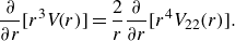 \begin{align} \frac {\partial }{\partial r}{ [ r^{3}V\!(r) ]}&=\frac {2}{r}\frac {\partial }{\partial r}{ [ r^{4}V_{22}(r) ]}. \end{align}
Appendix C. Relationships between one-dimensional spatial and spectral energy- density functions
For analysis of empirical data, it is useful to obtain relationships between the spectral and spatial variants of the one-dimensional energy-density functions. In the direction
 $\boldsymbol{r}=r_{1} \boldsymbol{\hat e}_{1}$
, the spectral one-dimensional energy-density functions are defined as
$\boldsymbol{r}=r_{1} \boldsymbol{\hat e}_{1}$
, the spectral one-dimensional energy-density functions are defined as
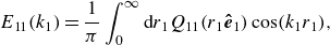 \begin{align} E_{11}(k_{1})&=\frac {1}{\pi } \int _{0}^{\infty }{\textrm d}r_{1}Q_{11}(r_{1}\boldsymbol{\hat e}_{1}) \cos (k_{1}r_{1}), \end{align}
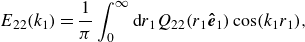 \begin{align} E_{22}(k_{1})&=\frac {1}{\pi } \int _{0}^{\infty }{\textrm d}r_{1}Q_{22}(r_{1}\boldsymbol{\hat e}_{1}) \cos (k_{1}r_{1}), \end{align}
 \begin{align} E_{33}(k_{1})&=\frac {1}{\pi } \int _{0}^{\infty }{\textrm d}r_{1}Q_{33}(r_{1}\boldsymbol{\hat e}_{1}) \cos (k_{1}r_{1}), \end{align}
and the inverse cosine transform transforms are
 \begin{align} Q_{11}(r_{1}\boldsymbol{\hat e}_{1})&= 2 \int _{0}^{\infty }{\textrm d}k_{1}E_{11}(k_{1})\cos (k_{1}r_{1}), \end{align}
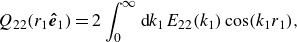 \begin{align} Q_{22}(r_{1}\boldsymbol{\hat e}_{1})&= 2 \int _{0}^{\infty }{\textrm d}k_{1}E_{22}(k_{1})\cos (k_{1}r_{1}), \end{align}
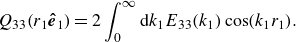 \begin{align} Q_{33}(r_{1}\boldsymbol{\hat e}_{1})&= 2 \int _{0}^{\infty }{\textrm d}k_{1}E_{33}(k_{1})\cos (k_{1}r_{1}). \end{align}
From the inverse transform pairs, it can be readily confirmed that
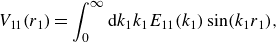 \begin{align} V_{11}(r_{1})&= \int _{0}^{\infty }{\textrm d}k_{1} k_{1}E_{11}(k_{1})\sin (k_{1}r_{1}), \end{align}
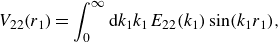 \begin{align} V_{22}(r_{1})&= \int _{0}^{\infty }{\textrm d}k_{1} k_{1}E_{22}(k_{1})\sin (k_{1}r_{1}), \end{align}
 \begin{align} V_{33}(r_{1})&= \int _{0}^{\infty }{\textrm d}k_{1} k_{1}E_{33}(k_{1})\sin (k_{1}r_{1}), \end{align}
and the associated forward transforms are
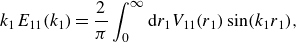 \begin{align} k_{1}E_{11}(k_{1})&=\frac {2}{\pi } \int _{0}^{\infty }{\textrm d}r_{1}V_{11}(r_{1})\sin (k_{1}r_{1}), \end{align}
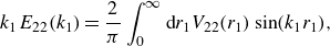 \begin{align} k_{1}E_{22}(k_{1})&=\frac {2}{\pi } \int _{0}^{\infty }{\textrm d}r_{1}V_{22}(r_{1})\sin (k_{1}r_{1}), \end{align}
 \begin{align} k_{1}E_{33}(k_{1})&=\frac {2}{\pi } \int _{0}^{\infty }{\textrm d}r_{1}V_{33}(r_{1})\sin (k_{1}r_{1}). \end{align}
Appendix D. Transport equation for
$\boldsymbol{V}\!(\boldsymbol{r},\boldsymbol{t})$

In the manuscript, we focused on kinematics of spatial energy-density functions. To study the dynamics, we can analyse their transport equations (Davidson & Pearson Reference Davidson and Pearson2005; Hamba Reference Hamba2015). As an illustration, here, focusing on homogeneous isotropic turbulence, we follow the approach of Davidson & Pearson (Reference Davidson and Pearson2005) to derive and analyse the transport equation for
 $V\!(r,t)$
, where
$V\!(r,t)$
, where
 $t$
is the time. (In the manuscript, we did not explicitly note the dependence on time as our focus was on kinematics.)
$t$
is the time. (In the manuscript, we did not explicitly note the dependence on time as our focus was on kinematics.)
Our starting point is the transport equation for
 $({1}/{2})Q_{ii}(r,t)$
, which is the Kármán–Howarth equation (Davidson Reference Davidson2004)
$({1}/{2})Q_{ii}(r,t)$
, which is the Kármán–Howarth equation (Davidson Reference Davidson2004)
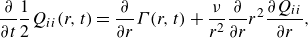 \begin{align} \frac {\partial }{\partial t}\frac {1}{2}Q_{ii}(r,t) &=\frac {\partial }{\partial r}\Gamma (r,t)+\frac {\nu }{r^{2}}\frac {\partial }{\partial r}r^{2}\frac {\partial Q_{ii}}{\partial {r}}, \end{align}
where
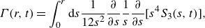 \begin{align} \Gamma (r,t)&=\int _{0}^{r}{\textrm d}s\frac {1}{12s^{2}} \frac {\partial }{\partial s}\frac {1}{s}\frac {\partial }{\partial s}{[ s^{4}S_{3}(s,t) ]} ,\end{align}
and the third-order structure function is defined as
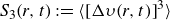 $S_{3}(r,t):=\langle {{ [ \Delta \upsilon (r,t) ]}^{3}} \rangle$
. Combining (D1) with (2.4)
$S_{3}(r,t):=\langle {{ [ \Delta \upsilon (r,t) ]}^{3}} \rangle$
. Combining (D1) with (2.4)
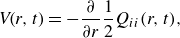 \begin{align} V\!(r,t)&=-\frac {\partial }{\partial r}\frac {1}{2}Q_{ii}(r,t), \end{align}
yields the transport equation for
 $V\!(r,t)$
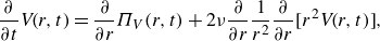 \begin{align} \frac {\partial }{\partial t}V\!(r,t)&=\frac {\partial }{\partial r}\Pi _{V}(r,t)+2\nu \frac {\partial }{\partial r} \frac {1}{r^{2}}\frac {\partial }{\partial r}{ [ r^{2}V\!(r,t) ]}, \end{align}
where we have defined the spatial energy flux
 $\Pi _{V}(r,t)$
as
$\Pi _{V}(r,t)$
as
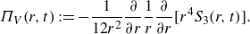 \begin{align} \Pi _{V}(r,t)&:=-\frac {1}{12r^{2}} \frac {\partial }{\partial r}\frac {1}{r}\frac {\partial }{\partial r}{[ r^{4}S_{3}(r,t) ]}. \end{align}
The spectral counterpart to (D4) is (Davidson Reference Davidson2004)
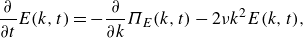 \begin{align} \frac {\partial }{\partial t}E(k,t)&=-\frac {\partial }{\partial k}\Pi _{E}(k,t)-2\nu k^{2}E(k,t), \end{align}
where
 $\Pi _{E}(k,t)$
is the spectral kinetic energy flux. In analogy with the spectral energy transfer
$\Pi _{E}(k,t)$
is the spectral kinetic energy flux. In analogy with the spectral energy transfer
 $T_{E}(k,t)=-{\partial \Pi _{E}}/{\partial }{k}$
, we can define the spatial energy transfer density function
$T_{E}(k,t)=-{\partial \Pi _{E}}/{\partial }{k}$
, we can define the spatial energy transfer density function
 \begin{align} T_{V}(r,t)&:=\frac {\partial \Pi _{V}}{\partial {r}}. \end{align}
It has the conservative property that
 $\int _{0}^{\infty } {\textrm d}r\, T_{V}=0$
.
$\int _{0}^{\infty } {\textrm d}r\, T_{V}=0$
.
It is instructive to consider the transfer of energy from eddies of size
 $\geqslant r$
to eddies of size
$\geqslant r$
to eddies of size
 $\leqslant r$
. To do this, we integrate (D4) over
$\leqslant r$
. To do this, we integrate (D4) over
 $r\to s\in [r,\infty ]$
for some arbitrary
$r\to s\in [r,\infty ]$
for some arbitrary
 $r$
$r$
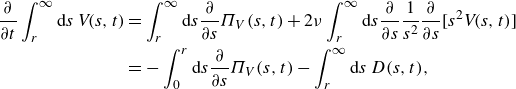 \begin{align} \frac {\partial }{\partial t}\int _{r}^{\infty }{\textrm d}s\, V\!(s,t)&=\int _{r}^{\infty }{\textrm d}s\frac {\partial }{\partial s}\Pi _{V}(s,t)+2\nu \int _{r}^{\infty }{\textrm d}s\frac {\partial }{\partial s}\frac {1}{s^{2}}\frac {\partial }{\partial s}{[ s^{2}V\!(s,t) ]}\nonumber \\ &=-\int _{0}^{r}{\textrm d}s\frac {\partial }{\partial s}\Pi _{V}(s,t)- \int _{r}^{\infty }{\textrm d}s\, D(s,t), \end{align}
where we have defined the dissipation density as
 \begin{align} D(r,t)&:=-2\nu \frac {\partial }{\partial r}\frac {1}{r^{2}}\frac {\partial }{\partial r}{[ r^{2}V\!(r,t) ]}. \end{align}
Equation (D8) can be interpreted as follows: the loss of energy from eddies of size
 $\geqslant r$
is due to the transfer to eddies of size
$\geqslant r$
is due to the transfer to eddies of size
 $\leqslant r$
(via
$\leqslant r$
(via
 $\Pi _{V}(r,t)$
) and direct loss to viscous dissipation (via
$\Pi _{V}(r,t)$
) and direct loss to viscous dissipation (via
 $D(r,t)$
). In other words, equation (D4) embodies an energy cascade in the real space.
$D(r,t)$
). In other words, equation (D4) embodies an energy cascade in the real space.
We can also analyse the inertial range. Integrating (D4) yields
 \begin{align} \int _{0}^{r}{\textrm d}s\, \frac {\partial }{\partial t}V\!(s,t)&=\Pi _{V}(r,t)+ \frac {2\nu }{r^{2}}\frac {\partial }{\partial r}{[ r^{2}V ]} -\lim _{r\to 0}\frac {2\nu }{r^{2}}\frac {\partial }{\partial r}{[ r^{2}V ]}. \end{align}
Next, recall that when the turbulence is locally isotropic, the velocity derivative moments are related by
 \begin{align} \left \langle {\frac {\partial u_{i}}{\partial {x_{j}}}\frac {\partial u_{i}}{\partial {x_{j}}}} \right \rangle &=-\left .{\frac {1}{r^{2}}\frac {\partial }{\partial r}{\left (r^{2}\frac {\partial Q_{ii}}{\partial r} \right )}}\right |_{r=0} =\langle {\boldsymbol{\omega }^{2}} \rangle , \end{align}
where
 $\langle {\boldsymbol{\omega }^{2}} \rangle$
is the mean enstrophy. This standard result can then be expressed in terms of the spatial energy density
$\langle {\boldsymbol{\omega }^{2}} \rangle$
is the mean enstrophy. This standard result can then be expressed in terms of the spatial energy density
 $V$
as
$V$
as
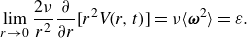 \begin{align} \lim _{r\to 0}\frac {2\nu }{r^{2}}\frac {\partial }{\partial r}{[ r^{2}V\!(r,t) ]} = \nu \langle {\boldsymbol{\omega }^{2}} \rangle =\varepsilon . \end{align}
Finally, substituting (D12) into (D10) we arrive at the integrated form of the transport equation
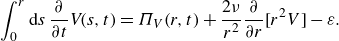 \begin{align} \int _{0}^{r}{\textrm d}s\, \frac {\partial }{\partial t}V\!(s,t)&=\Pi _{V}(r,t)+ \frac {2\nu }{r^{2}}\frac {\partial }{\partial r}{ [ r^{2}V ]} -\varepsilon . \end{align}
Now, focusing on the inertial-range eddies, we invoke the standard assumptions that the turbulence is locally stationary (so the time-derivative term on the left-hand size is zero) and that the viscous term is negligible. This yields the scale invariance of the spatial energy flux in the inertial range
 \begin{align} \Pi _{V}(r,t)&=\varepsilon . \end{align}


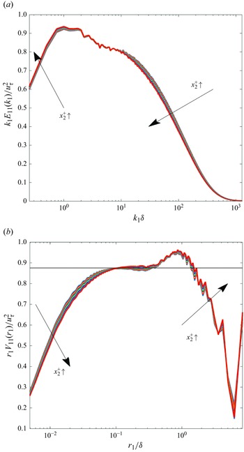


 Open access