





1. Introduction
1.1. Modelling surface roughness in a transitionally rough regime
Flows over rough surfaces are critically important due to their extensive engineering applications. However, with the multitude of roughness topographies and the prohibitive costs associated with testing each of the surfaces, the accurate understanding of flow modifications and the prediction of the drag caused by the rough surfaces remain an important challenge. The uncertainties stemming from the limited knowledge of flow modifications due to rough surfaces and unreliable drag predictions result in significant financial losses, amounting to billions of dollars annually (Schultz et al. Reference Schultz, Bendick, Holm and Hertel2011; Stevens & Meneveau Reference Stevens and Meneveau2017; Chung et al. Reference Chung, Hutchins, Schultz and Flack2021). Consequently, an increasing number of numerical studies focus on rough-wall bounded turbulent flows. An approach is to consider the full geometry of the rough surfaces, so that all essential small-scale flow characteristics are captured (e.g. Leonardi et al. Reference Leonardi, Orlandi, Smalley, Djenidi and Antonia2003; Orlandi, Leonardi & Antonia Reference Orlandi, Leonardi and Antonia2006; Forooghi et al. Reference Forooghi, Stroh, Schlatter and Frohnapfel2018; Abderrahaman-Elena, Fairhall & García-Mayoral Reference Abderrahaman-Elena, Fairhall and García-Mayoral2019).
However, resolving the full texture of rough surfaces using direct numerical simulations (DNS) is prohibitively expensive. Another approach taken in the past is therefore based on the characterisation of the effects of rough surfaces by focusing on physically meaningful flow parameters rather than delving into the intricate details of the flow within the textured region. This is particularly useful for the low to intermediate range of transitional roughness ( $5 \leqslant k_s^+ \leqslant 20$
, where
$5 \leqslant k_s^+ \leqslant 20$
, where $k_s^+$
is the equivalent sand-grain roughness, with the superscript
$k_s^+$
is the equivalent sand-grain roughness, with the superscript $+$
denoting the viscous inner scaling), in which changes in drag are primarily a consequence of the viscous modifications induced by the surface roughness. In doing this, the concepts of ‘protrusion height’ and ‘slip length’ were introduced. Bechert & Bartenwerfer (Reference Bechert and Bartenwerfer1989) observed a mean longitudinal flow over the riblet from a depth beneath the riblet tips, and called this distance from the riblets tips the ‘protrusion height’. Luchini, Manzo & Pozzi (Reference Luchini, Manzo and Pozzi1991) subsequently observed that the protrusion height of the cross-flow over the riblets was smaller than that of the longitudinal flow, with their resulting difference characterising the variations in drag. The ‘slip lengths’ have proven to be useful in modelling the effects of superhydrophobic surfaces on turbulent flows using the Navier slip boundary conditions (e.g. Lauga & Stone Reference Lauga and Stone2003; Min & Kim Reference Min and Kim2004; Busse & Sandham Reference Busse and Sandham2012; Fairhall, Abderrahaman-Elena & García-Mayoral Reference Fairhall, Abderrahaman-Elena and García-Mayoral2019). Later, it was established that the protrusion heights and slip lengths are conceptually equivalent (Luchini Reference Luchini2015; Garcia-Mayoral et al. Reference García-Mayoral, Gómez-de-Segura and Fairhall2019).
$+$
denoting the viscous inner scaling), in which changes in drag are primarily a consequence of the viscous modifications induced by the surface roughness. In doing this, the concepts of ‘protrusion height’ and ‘slip length’ were introduced. Bechert & Bartenwerfer (Reference Bechert and Bartenwerfer1989) observed a mean longitudinal flow over the riblet from a depth beneath the riblet tips, and called this distance from the riblets tips the ‘protrusion height’. Luchini, Manzo & Pozzi (Reference Luchini, Manzo and Pozzi1991) subsequently observed that the protrusion height of the cross-flow over the riblets was smaller than that of the longitudinal flow, with their resulting difference characterising the variations in drag. The ‘slip lengths’ have proven to be useful in modelling the effects of superhydrophobic surfaces on turbulent flows using the Navier slip boundary conditions (e.g. Lauga & Stone Reference Lauga and Stone2003; Min & Kim Reference Min and Kim2004; Busse & Sandham Reference Busse and Sandham2012; Fairhall, Abderrahaman-Elena & García-Mayoral Reference Fairhall, Abderrahaman-Elena and García-Mayoral2019). Later, it was established that the protrusion heights and slip lengths are conceptually equivalent (Luchini Reference Luchini2015; Garcia-Mayoral et al. Reference García-Mayoral, Gómez-de-Segura and Fairhall2019).
The concepts of protrusion height and slip length are primarily used to model the effect of the roughness texture on the velocity components parallel to the wall combining with the Navier slip boundary conditions. However, by construction, they do not appropriately capture the wall-normal momentum transport (Gómez-de-Segura et al. Reference Gómez-de-Segura, Fairhall, MacDonald, Chung and Garcia-Mayoral2018; Bottaro Reference Bottaro2019; Zampogna, Magnaudet & Bottaro Reference Zampogna, Magnaudet and Bottaro2019). To address this limitation, the transpiration-resistance model (TRM) for boundary conditions was recently proposed by Lācis et al. (Reference Lācis, Sudhakar, Pasche and Bagheri2020) and subsequently applied to turbulent flows over rough surfaces (Sudhakar et al. Reference Sudhakar, Lācis, Pasche and Bagheri2021; Khorasani et al. Reference Khorasani, Lācis, Pasche, Rosti and Bagheri2022). The TRM boundary conditions integrate the slip conditions for the wall-parallel velocity components with a transpiration condition for the wall-normal velocity, so that the changes in wall-normal velocity are coupled to the shear variations of the other two velocity components (Lācis et al. Reference Lācis, Sudhakar, Pasche and Bagheri2020). Furthermore, both Lācis et al. (Reference Lācis, Sudhakar, Pasche and Bagheri2020) and Sudhakar et al. (Reference Sudhakar, Lācis, Pasche and Bagheri2021) have shown that the TRM boundary conditions well capture the effects of real surface roughness in viscous-dominated flows. Utilising the TRM boundary model, Khorasani et al. (Reference Khorasani, Lācis, Pasche, Rosti and Bagheri2022) successfully reproduced the homogeneous geometrical roughness effects in low and intermediate ranges of the transitional rough regime.
1.2. Linear and quasi-linear modelling for wall-bounded turbulence
A growing number of linear modelling approaches have recently been developed for wall-bounded turbulent flows. Early studies considered the linearised Navier–Stokes equations around the turbulent mean velocity, typically linearly stable in wall-bounded turbulence, and studied the transient amplification mechanism to understand the origin of coherent structures (Butler & Farrell Reference Butler and Farrell1993; Chernyshenko & Baig Reference Chernyshenko and Baig2005; Del Alamo & Jimenez Reference Del Alamo and Jimenez2006; Pujals et al. Reference Pujals, García-Villalba, Cossu and Depardon2009). In a similar context, some variants of this approach have been formulated, and well-known examples include input–output analysis (Hwang & Cossu Reference Hwang and Cossu2010; McKeon & Sharma Reference McKeon and Sharma2010; Zare, Jovanović & Georgiou Reference Zare, Jovanović and Georgiou2017). These approaches have also been used for flows with surface manipulations, e.g. spanwise wall oscillation (Moarref & Jovanović Reference Moarref and Jovanović2012), opposition control (Luhar, Sharma & McKeon Reference Luhar, Sharma and McKeon2014) and riblets (Chavarin & Luhar Reference Chavarin and Luhar2020; Ran, Zare & Jovanović Reference Ran, Zare and Jovanović2021). Despite the successful applications for flow modelling, these approaches typically predict the flow behaviours mainly through the gain that characterises the amplification of the optimal input (initial condition or forcing) for the resulting output, not providing useful measures that can be obtained through DNS or experiments: e.g. drag reduction or changes in turbulence statistics. Some notable exceptions to this are those of Moarref & Jovanović (Reference Moarref and Jovanović2012) and Ran et al. (Reference Ran, Zare and Jovanović2021), where a Reynolds-averaged Navier–Stokes (RANS) model is passively coupled, and Zampino et al. (Reference Zampino, Lasagna and Ganapathisubramani2022), who used linearised RANS equations coupled with the Spalart–Allmaras transport equation to investigate secondary currents in turbulent channel flow.
Recently, some new efforts have been made to incorporate the nonlinearity of the Navier–Stokes equations into the linear modelling approaches in a minimal manner using the framework of ‘quasi-linear’ approximation. This approach was introduced by Hwang & Eckhardt (Reference Hwang and Eckhardt2020) and has been referred to as the ‘minimal quasi-linear approximation’ (MQLA). In this approach, the full nonlinear mean equation is considered, while the fluctuation equations are linearised around the mean velocity. The nonlinear self-interaction terms in the fluctuations equations are subsequently modelled using an empirical eddy viscosity model and stochastic forcing. Assuming that the mean velocity is empirically known (e.g. Cess Reference Cess1958), the stochastic forcing is determined self-consistently by making the Reynolds shear stresses from the fluctuation equations numerically identical to those from the mean velocity. This approach was shown to reproduce all the behaviours of second-order turbulence statistics qualitatively well even at extremely high Reynolds numbers (Skouloudis & Hwang Reference Skouloudis and Hwang2022).
In MQLA, only spanwise variations in plane wavenumbers were considered, as it was originally intended to relate it to the classical attached eddy model of Townsend (Reference Townsend1976). Efforts for MQLA to include all plane wavenumbers were subsequently made (Holford, Lee & Hwang Reference Holford, Lee and Hwang2024a ). Using the self-similarity in the velocity spectra with respect to the distance from the wall in the logarithmic region (Hwang Reference Hwang2015), the self-similar forcing spectra were assimilated from DNS data (Holford, Lee & Hwang Reference Holford, Lee and Hwang2023). These forcings were then incorporated into the quasi-linear approximation framework of Hwang & Eckhardt (Reference Hwang and Eckhardt2020). Compared to MQLA, this extended framework, referred to as the data-driven approximation (DQLA), provides significant quantitative improvements on the predictions of turbulence intensities with a largely reduced anisotropy (Holford et al. Reference Holford, Lee and Hwang2024a ). It also offers the full two-dimensional (2-D) plane wavenumber spectra, the scaling behaviour of which is consistent with that from DNS (Hwang Reference Hwang2024).
1.3. Scope
Given the high computational demands to capture the roughness effects in the scale of the surface texture elements, the objective of the present study is to develop a quasi-linear approximation framework of Hwang & Eckhardt (Reference Hwang and Eckhardt2020) and Holford et al. (Reference Holford, Lee and Hwang2024a ) in the presence of (mildly) rough surfaces modelled by the TRM boundary conditions on the wall without detailed geometrical representations of the surface roughness. Particular attention is paid to model-based predictions for roughness functions, frequently used in the surface roughness research community (Chung et al. Reference Chung, Hutchins, Schultz and Flack2021), at a computational cost much lower than that of DNS with TRM boundary conditions. For this purpose, apart from considering both MQLA and DQLA, we further introduce a new variant of this approach designed to provide turbulence statistics better than those of MQLA at a computational cost much lower than that of DQLA. In this framework, an implicit assumption is imposed that the flow remains smooth-wall-like, with turbulent structures near the wall that are not largely modified. In this sense, the nonlinear self-interaction terms are modelled with the eddy viscosity model and stochastic forcing used for smooth walls. From the given modelling efforts, we will see that the proposed quasi-linear modelling approaches here offer encouraging predictions for the roughness functions compared to those of DNS (Khorasani et al. Reference Khorasani, Lācis, Pasche, Rosti and Bagheri2022) in the lower part of the transitional rough regime with moderate TRM boundary conditions.
This paper is organised as follows. In § 2, we briefly introduce the previous quasi-linear approximations for no-slip boundary conditions, and subsequently establish an approach to predict turbulence statistics and spectra with the TRM boundary conditions. In § 3, the roughness functions, turbulence statistics and velocity spectra predicted by the established quasi-linear approximations are compared with those from DNS (Khorasani et al. Reference Khorasani, Lācis, Pasche, Rosti and Bagheri2022), demonstrating the capability of the proposed modelling approaches here. Using the encouraging results in § 3, the behaviour of the roughness function for the mean velocity is explored in a wide range of parameter space in § 4. Finally, conclusions and perspectives of the present study are provided in § 5.
2. Problem formulation
2.1. Equations of motion
We begin by introducing the equations of motion for the quasi-linear approximation of Hwang & Eckhardt (Reference Hwang and Eckhardt2020) in fully-developed incompressible turbulent channel flow, bounded by two plates that are infinitely long and wide. Here, the streamwise, wall-normal and spanwise coordinates are denoted as $x$
,
$x$
, $y$
and
$y$
and $z$
, respectively, and the corresponding velocity vector is represented as
$z$
, respectively, and the corresponding velocity vector is represented as $\boldsymbol{u} = (u, v, w)$
. The channel half-height is set as
$\boldsymbol{u} = (u, v, w)$
. The channel half-height is set as $h$
, and the two plates are located at
$h$
, and the two plates are located at $y = 0, 2h$
, respectively. To implement the quasi-linear approximation, the velocity field is decomposed into a time-averaged mean
$y = 0, 2h$
, respectively. To implement the quasi-linear approximation, the velocity field is decomposed into a time-averaged mean $\boldsymbol{U} = (U(y), 0, 0)$
, and fluctuations about this mean
$\boldsymbol{U} = (U(y), 0, 0)$
, and fluctuations about this mean $\boldsymbol{u}' = (u', v', w')$
: i.e. the Reynolds decomposition. This yields the following coupled equations for the mean and fluctuations:
$\boldsymbol{u}' = (u', v', w')$
: i.e. the Reynolds decomposition. This yields the following coupled equations for the mean and fluctuations:
 \begin{align}&\qquad\qquad\qquad \nu \frac {{\rm d}U}{{\rm d}y}-\overline {u'v'} = \frac {\tau _w}{\rho }\left(1-\frac {y}{h}\right), \end{align}
 \begin{align}& \frac {\partial \boldsymbol{u}'}{\partial t}+ (\boldsymbol{U} \boldsymbol{\cdot} \boldsymbol{\nabla} )\boldsymbol{u}' + (\boldsymbol{u}'\boldsymbol{\cdot} \boldsymbol{\nabla} ) \boldsymbol{U} =-\frac {1}{\rho }\,\boldsymbol{\nabla} {p'}+\nu\, {\nabla} ^2 {\boldsymbol{u}'}+ \boldsymbol{N}, \end{align}
where
 \begin{equation} \boldsymbol{N} = -\boldsymbol{\nabla} \boldsymbol{\cdot} \left(\boldsymbol{u}'\boldsymbol{u}'-\overline {\boldsymbol{u}'\boldsymbol{u}'}\right). \end{equation}
Here, $t$
denotes time and
$t$
denotes time and $\overline {({\cdot} )}$
represents the average in time and two homogeneous directions, with
$\overline {({\cdot} )}$
represents the average in time and two homogeneous directions, with $\tau _w$
the time-averaged wall shear stress,
$\tau _w$
the time-averaged wall shear stress, $p'$
the fluctuating pressure,
$p'$
the fluctuating pressure, $\rho$
the fluid density, and
$\rho$
the fluid density, and $\nu$
the kinematic viscosity. In the present study, the effects of roughness on near-wall turbulence are modelled with the TRM boundary conditions (e.g. Lācis et al. Reference Lācis, Sudhakar, Pasche and Bagheri2020). The boundary conditions for the turbulent mean velocity are written as
$\nu$
the kinematic viscosity. In the present study, the effects of roughness on near-wall turbulence are modelled with the TRM boundary conditions (e.g. Lācis et al. Reference Lācis, Sudhakar, Pasche and Bagheri2020). The boundary conditions for the turbulent mean velocity are written as
 \begin{equation} {U} =l_x\left .\frac {\partial {U}}{\partial y}\right \vert _{y=0,2h}, \end{equation}
and the fluctuating velocities at the two boundaries $y=0,2h$
are defined as
$y=0,2h$
are defined as
 \begin{align}&\qquad\qquad\,\, {u'} =l_x\left .\frac {\partial {u'}}{\partial y}\right \vert _{y=0,2h}, \end{align}
 \begin{align}&\qquad\qquad {w'} =l_z\left .\frac {\partial {w'}}{\partial y}\right \vert _{y=0,2h}, \end{align}
 \begin{align}& {v'} =-m_x\left .\frac {\partial {u'}}{\partial x}\right \vert _{y=0,2h}-m_z \left .\frac {\partial {w'}}{\partial z}\right \vert _{y=0,2h}, \end{align}
where the coefficients $l_x$
,
$l_x$
, $l_z$
,
$l_z$
, $m_x$
and
$m_x$
and $m_z$
are slip and transpiration lengths, respectively. The TRM boundary conditions not only incorporate the Navier-slip boundary conditions for the streamwise and spanwise velocities, but also provide a transpiration condition for the wall-normal velocity that accounts for the wall-normal momentum transport associated with the surface texture through the transpiration lengths. It has been shown that these boundary conditions model well for the rough surfaces in the transitionally rough regime, which do not significantly modify the near-wall turbulence. From this perspective, it is ideal to test the modelling capacity of the quasi-linear approximations developed for smooth walls (Hwang & Eckhardt Reference Hwang and Eckhardt2020; Holford et al. Reference Holford, Lee and Hwang2024a
).
$m_z$
are slip and transpiration lengths, respectively. The TRM boundary conditions not only incorporate the Navier-slip boundary conditions for the streamwise and spanwise velocities, but also provide a transpiration condition for the wall-normal velocity that accounts for the wall-normal momentum transport associated with the surface texture through the transpiration lengths. It has been shown that these boundary conditions model well for the rough surfaces in the transitionally rough regime, which do not significantly modify the near-wall turbulence. From this perspective, it is ideal to test the modelling capacity of the quasi-linear approximations developed for smooth walls (Hwang & Eckhardt Reference Hwang and Eckhardt2020; Holford et al. Reference Holford, Lee and Hwang2024a
).
The mean equation (2.1a
) includes the Reynolds shear stress term that feeds back from the fluctuating velocity field. The equation for the fluctuating velocity (2.1b
) is of the form linearised about the mean velocity if the nonlinear term $\boldsymbol{N}$
is dropped. Following Hwang & Eckhardt (Reference Hwang and Eckhardt2020) and Holford et al. (Reference Holford, Lee and Hwang2024a
), the nonlinear term
$\boldsymbol{N}$
is dropped. Following Hwang & Eckhardt (Reference Hwang and Eckhardt2020) and Holford et al. (Reference Holford, Lee and Hwang2024a
), the nonlinear term $\boldsymbol{N}$
is modelled as
$\boldsymbol{N}$
is modelled as
 \begin{equation} \boldsymbol{N}_{\nu _t,f} = \boldsymbol{\nabla} \boldsymbol{\cdot} \big(\nu _t \big(\boldsymbol{\nabla} \boldsymbol{u}'+ \boldsymbol{\nabla} {\boldsymbol{u}'}^{\rm T}\big)\big)+\boldsymbol{f}', \end{equation}
where the eddy viscosity $\nu _t$
is adopted from the empirical expression of Cess (Reference Cess1958),
$\nu _t$
is adopted from the empirical expression of Cess (Reference Cess1958),
 \begin{equation} \nu _t(\eta ) = \frac {\nu }{2} \left\{1+\frac {\kappa ^2\,Re_{\tau }^2}{9}\left(1-\eta ^2\right)^2\left(1+2\eta ^2\right)^2(1-\exp[(|\eta |-1)\,Re_{\tau }/A])^2\right\}-\frac {\nu }{2}, \end{equation}
with $\eta = (y-h)/h$
, and
$\eta = (y-h)/h$
, and $\boldsymbol{f}'=(f'_u,f'_v,f'_w)$
is a stochastic forcing term whose amplitude and colour are to be determined. Here, the eddy viscosity parameters are set to
$\boldsymbol{f}'=(f'_u,f'_v,f'_w)$
is a stochastic forcing term whose amplitude and colour are to be determined. Here, the eddy viscosity parameters are set to $\kappa = 0.426$
and
$\kappa = 0.426$
and $A = 25.4$
, with which the best least squares fitting of the mean velocity profile of (2.1a
) is obtained with that of DNS at
$A = 25.4$
, with which the best least squares fitting of the mean velocity profile of (2.1a
) is obtained with that of DNS at $Re_{\tau }\approx 2000$
(Del Alamo & Jimenez Reference Del Alamo and Jimenez2006). The inclusion of the eddy viscosity term in (2.4a
) has been understood to significantly simplify the modelling process, and consolidates the key physical elements, as recently analysed in detail by Holford et al. (Reference Holford, Lee and Hwang2024b
) through a comparison of spectral energy budgets between DNS and quasi-linear approximations. Furthermore, the eddy viscosity term has been consistently shown to enhance the capacity of (2.1b
) for the predictions of turbulent statistics and energy spectra, as well as for the performance of state estimations (Hwang Reference Hwang2016; Illingworth, Monty & Marusic Reference Illingworth, Monty and Marusic2018; Madhusudanan, Illingworth & Marusic Reference Madhusudanan, Illingworth and Marusic2019; Towne, Lozano-Durán & Yang Reference Towne, Lozano-Durán and Yang2020; Holford et al. Reference Holford, Lee and Hwang2023).
$Re_{\tau }\approx 2000$
(Del Alamo & Jimenez Reference Del Alamo and Jimenez2006). The inclusion of the eddy viscosity term in (2.4a
) has been understood to significantly simplify the modelling process, and consolidates the key physical elements, as recently analysed in detail by Holford et al. (Reference Holford, Lee and Hwang2024b
) through a comparison of spectral energy budgets between DNS and quasi-linear approximations. Furthermore, the eddy viscosity term has been consistently shown to enhance the capacity of (2.1b
) for the predictions of turbulent statistics and energy spectra, as well as for the performance of state estimations (Hwang Reference Hwang2016; Illingworth, Monty & Marusic Reference Illingworth, Monty and Marusic2018; Madhusudanan, Illingworth & Marusic Reference Madhusudanan, Illingworth and Marusic2019; Towne, Lozano-Durán & Yang Reference Towne, Lozano-Durán and Yang2020; Holford et al. Reference Holford, Lee and Hwang2023).
As discussed earlier, the formulation of the quasi-linear approximations in this study requires a known mean velocity. Indeed, like RANS, (2.1) has a closure problem due to unknown $\boldsymbol{N}$
– if
$\boldsymbol{N}$
– if $\boldsymbol{N}$
is known, then (2.1) is solvable to obtain the mean and fluctuating velocities. Conversely, if part of the solution, say the mean velocity, is assumed to be known, then it is possible to construct
$\boldsymbol{N}$
is known, then (2.1) is solvable to obtain the mean and fluctuating velocities. Conversely, if part of the solution, say the mean velocity, is assumed to be known, then it is possible to construct $\boldsymbol{N}$
inversely, although
$\boldsymbol{N}$
inversely, although $\boldsymbol{N}$
is not necessarily unique (Skouloudis & Hwang Reference Skouloudis and Hwang2022; see also § 2.2). This is the central theoretical element of the present quasi-linear approximations. In the present study, the construction of
$\boldsymbol{N}$
is not necessarily unique (Skouloudis & Hwang Reference Skouloudis and Hwang2022; see also § 2.2). This is the central theoretical element of the present quasi-linear approximations. In the present study, the construction of $\boldsymbol{N}$
is performed using
$\boldsymbol{N}$
is performed using $\boldsymbol{N}_{\nu _t,f}$
in (2.4), where the stochastic forcing term is determined with the known mean velocity. The mean velocity here is obtained by solving (2.1a
), with the well-known eddy-viscosity-based closure given by
$\boldsymbol{N}_{\nu _t,f}$
in (2.4), where the stochastic forcing term is determined with the known mean velocity. The mean velocity here is obtained by solving (2.1a
), with the well-known eddy-viscosity-based closure given by $-\overline {u'v'}=\nu _t\, {{\rm d}U}/{{\rm d}y}$
with
$-\overline {u'v'}=\nu _t\, {{\rm d}U}/{{\rm d}y}$
with $\nu _t$
in (2.4b
).
$\nu _t$
in (2.4b
).
2.2. Forcing models
To apply the framework of the stochastic linear dynamical system for (2.1b
) (Farrell & Ioannou Reference Farrell and Ioannou1993; Jovanović & Bamieh Reference Jovanović and Bamieh2005; Hwang & Cossu Reference Hwang and Cossu2010), we initially consider that the forcing is temporally white and spatially and componentwisely uncorrelated. Given the homogeneous nature in the wall-parallel directions, we perform the Fourier transform along the $x$
and
$x$
and $z$
directions,
$z$
directions,
 \begin{equation} \,\hat {\!\boldsymbol{f}}'(t,y;k_x,k_z)=\int _{-\infty }^{\infty }\int _{-\infty }^{\infty } \boldsymbol{f}'(t,x,y,z)\,{\rm e}^{-{\rm i}(k_xx+k_zz)}\,{\rm d}x\,{\rm d}z, \end{equation}
where $\hat {(\cdot)}$
denotes the Fourier transformed state, and
$\hat {(\cdot)}$
denotes the Fourier transformed state, and $(k_x, k_z)$
is the considered wavenumber pair with the streamwise and spanwise wavelengths denoted as
$(k_x, k_z)$
is the considered wavenumber pair with the streamwise and spanwise wavelengths denoted as $\lambda _x = 2\pi /k_x$
and
$\lambda _x = 2\pi /k_x$
and $\lambda _z = 2\pi /k_z$
, respectively. The same definitions of the Fourier transform are used for the other flow variables. Then the spectral covariance matrix of the stochastic forcing is set to be given by
$\lambda _z = 2\pi /k_z$
, respectively. The same definitions of the Fourier transform are used for the other flow variables. Then the spectral covariance matrix of the stochastic forcing is set to be given by
 \begin{equation} \begin{aligned} &E\left[\,\hat {\!\boldsymbol{f}}'(t,y;k_x,k_z)\,\hat {\!\boldsymbol{f}}'^H(t',y';k_x,k_z)\right]\\&= \begin{bmatrix} W_{u}(k_x,k_z) &0 &0\\[4pt] 0& W_{v}(k_x,k_z) &0\\[4pt] 0 &0 & W_{w}(k_x,k_z) \end{bmatrix} \delta (y-y')\,\delta (t-t'), \end{aligned} \end{equation}
where $(\cdot)^H$
denotes the complex conjugate transpose,
$(\cdot)^H$
denotes the complex conjugate transpose, $E[\cdot]$
is the expectation operator on different stochastic realisations,
$E[\cdot]$
is the expectation operator on different stochastic realisations, $\delta (\cdot)$
is the Dirac delta function, and
$\delta (\cdot)$
is the Dirac delta function, and $W_{l}$
with
$W_{l}$
with $l=\{u,v,w\}$
are component weights as functions of
$l=\{u,v,w\}$
are component weights as functions of $k_x$
and
$k_x$
and $k_z$
, through which the amplitude of the stochastic forcing is determined in the streamwise and spanwise directions.
$k_z$
, through which the amplitude of the stochastic forcing is determined in the streamwise and spanwise directions.
The following spectral (spatial and componentwise) covariance matrix of velocity fluctuations can be computed by solving (2.1b ) in the Fourier space, if the stochastic forcing is specified:
 \begin{equation} \phi _{\boldsymbol{\it uu}}\left(y,y';k_x,k_z\right)=E\left[\hat {\boldsymbol{u}}'(t,y;k_x,k_z)\,\hat {\boldsymbol{u}}'^H(t,y';k_x,k_z)\right]. \end{equation}
Given the existence of a linear relationship between the velocity and forcing spectral covariance matrices, $\phi _{\boldsymbol{\it uu}}(y,y'; k_x,k_z)$
is written as
$\phi _{\boldsymbol{\it uu}}(y,y'; k_x,k_z)$
is written as
 \begin{equation} \phi _{\boldsymbol{\it uu}}(y,y';k_x,k_z)=\sum _{{l}=u,v,w} W_{{l}}(k_x,k_z)\, \phi _{\boldsymbol{\it uu},l}(y,y';k_x,k_z), \end{equation}
where $\phi _{\boldsymbol{\it uu},l}(y,y';k_x,k_z)$
is the velocity spectral covariance matrix corresponding to each component of the forcing with the unit amplitude (Holford et al. Reference Holford, Lee and Hwang2024a
). In particular, using the linear nature of (2.4a
),
$\phi _{\boldsymbol{\it uu},l}(y,y';k_x,k_z)$
is the velocity spectral covariance matrix corresponding to each component of the forcing with the unit amplitude (Holford et al. Reference Holford, Lee and Hwang2024a
). In particular, using the linear nature of (2.4a
), $\phi _{\boldsymbol{\it uu},l}(y,y';k_x,k_z)$
in (2.8) is obtained from the linear response to the white-in-time forcing with the unit amplitude (i.e. setting
$\phi _{\boldsymbol{\it uu},l}(y,y';k_x,k_z)$
in (2.8) is obtained from the linear response to the white-in-time forcing with the unit amplitude (i.e. setting $W_{{l}}(k_x,k_z)=1$
for each
$W_{{l}}(k_x,k_z)=1$
for each $l\ (=u,v,w)$
). For instance,
$l\ (=u,v,w)$
). For instance, $\phi _{\boldsymbol{\it uu},u}(y,y';k_x,k_z)$
in (2.8) is the velocity spectral covariance matrix computed with the forcing
$\phi _{\boldsymbol{\it uu},u}(y,y';k_x,k_z)$
in (2.8) is the velocity spectral covariance matrix computed with the forcing
 \begin{equation} \begin{aligned} E[&\,\hat {\!\boldsymbol{f}}'(t,y;k_x,k_z)\,\hat {\!\boldsymbol{f}}'^H(t',y';k_x,k_z)]= \begin{bmatrix} \delta (y-y') &0&0\\ 0& 0 &0\\ 0 &0 & 0 \end{bmatrix} \delta (t-t'). \end{aligned} \end{equation}
The stochastic forcing in (2.6) serves as a starting point for the quasi-linear approximation approach here. With the pre-computed $\phi _{\boldsymbol{\it uu},l}(y,y';k_x,k_z)$
, the remaining problem becomes the determination of
$\phi _{\boldsymbol{\it uu},l}(y,y';k_x,k_z)$
, the remaining problem becomes the determination of $W_l$
in such a way that the resulting Reynolds shear stress corresponds to that in (2.1) using the prescribed mean velocity (for the details, see Holford et al. Reference Holford, Lee and Hwang2024a
). However, a forcing that is white in time and decorrelated in the wall-normal direction for each
$W_l$
in such a way that the resulting Reynolds shear stress corresponds to that in (2.1) using the prescribed mean velocity (for the details, see Holford et al. Reference Holford, Lee and Hwang2024a
). However, a forcing that is white in time and decorrelated in the wall-normal direction for each $k_x$
and
$k_x$
and $k_z$
is physically unrealistic. Indeed, this kind of forcing covariance has previously been shown to generate a non-physical large energy response in the region close to the channel centre (Hwang & Eckhardt Reference Hwang and Eckhardt2020; Holford et al. Reference Holford, Lee and Hwang2024a
). It has been proposed that a simple ad hoc solution to this is considering some of the leading proper orthogonal decomposition (POD) modes from the response to the stochastic forcing, which can capture the primary energy-containing motions at integral length scales – the reader may refer to Hwang & Eckhardt (Reference Hwang and Eckhardt2020) and Holford et al. (Reference Holford, Lee and Hwang2024b
), where the origin of the non-physical stochastic response, the effect of the number of the POD modes, and the related energetics are fully discussed for the quasi-linear approximations considered here. Employing this approach, the velocity spectral covariance matrix is further approximated by considering some of the leading POD modes from
$k_z$
is physically unrealistic. Indeed, this kind of forcing covariance has previously been shown to generate a non-physical large energy response in the region close to the channel centre (Hwang & Eckhardt Reference Hwang and Eckhardt2020; Holford et al. Reference Holford, Lee and Hwang2024a
). It has been proposed that a simple ad hoc solution to this is considering some of the leading proper orthogonal decomposition (POD) modes from the response to the stochastic forcing, which can capture the primary energy-containing motions at integral length scales – the reader may refer to Hwang & Eckhardt (Reference Hwang and Eckhardt2020) and Holford et al. (Reference Holford, Lee and Hwang2024b
), where the origin of the non-physical stochastic response, the effect of the number of the POD modes, and the related energetics are fully discussed for the quasi-linear approximations considered here. Employing this approach, the velocity spectral covariance matrix is further approximated by considering some of the leading POD modes from $\phi _{\boldsymbol{\it uu},l}(y,y';k_x,k_z)$
in (2.8):
$\phi _{\boldsymbol{\it uu},l}(y,y';k_x,k_z)$
in (2.8):
 \begin{equation} \phi _{\boldsymbol{\it uu},l}^{\textit{POD}}(y,y';k_x,k_z) \approx \sum _{i=1}^{N_{\textit{POD}}} \sigma _i\, \hat {\boldsymbol{u}}_{i,POD}(y;k_x,k_z)\,\hat {\boldsymbol{u}}_{i,POD}^H(y';k_x,k_z), \end{equation}
where $N_{\textit{POD}}$
is the number of the considered leading POD modes, and
$N_{\textit{POD}}$
is the number of the considered leading POD modes, and $\sigma _i$
and
$\sigma _i$
and $\hat {\boldsymbol{u}}_{i,POD}$
are the eigenvalues and eigenfunctions of the velocity spectral covariance matrix obtained from the white-in-time and spatially decorrelated forcing
$\hat {\boldsymbol{u}}_{i,POD}$
are the eigenvalues and eigenfunctions of the velocity spectral covariance matrix obtained from the white-in-time and spatially decorrelated forcing $\phi _{\boldsymbol{\it uu},l}(y,y';k_x,k_z)$
in (2.8). Based on previous findings (Hwang & Eckhardt Reference Hwang and Eckhardt2020; Holford et al. Reference Holford, Lee and Hwang2024a
),
$\phi _{\boldsymbol{\it uu},l}(y,y';k_x,k_z)$
in (2.8). Based on previous findings (Hwang & Eckhardt Reference Hwang and Eckhardt2020; Holford et al. Reference Holford, Lee and Hwang2024a
), $N_{\textit{POD}} = 2$
is considered in this study.
$N_{\textit{POD}} = 2$
is considered in this study.
Following Holford et al. (Reference Holford, Lee and Hwang2024a
), the forcing weight $W_{l}(k_x,k_z)$
for each component is further prescribed in the form
$W_{l}(k_x,k_z)$
for each component is further prescribed in the form
 \begin{equation} W_{l}(k_x,k_z)=W_{l,k_x}(k_x/k_z)\,W_{k_z}(k_z). \end{equation}
Here, the self-similar streamwise weight $W_{l,k_x}(k_x/k_z)$
is used to account for the self-similar nature of the energy-containing part in the velocity and forcing spectra (i.e. the attached eddy hypothesis; for further details, see Holford et al. Reference Holford, Lee and Hwang2023), and
$W_{l,k_x}(k_x/k_z)$
is used to account for the self-similar nature of the energy-containing part in the velocity and forcing spectra (i.e. the attached eddy hypothesis; for further details, see Holford et al. Reference Holford, Lee and Hwang2023), and $W_{k_z}(k_z)$
is used to determine the forcing amplitude for each spanwise scale that varies from the near-wall (
$W_{k_z}(k_z)$
is used to determine the forcing amplitude for each spanwise scale that varies from the near-wall ( $\lambda _z^+ \approx O(100)$
) to the outer one (
$\lambda _z^+ \approx O(100)$
) to the outer one ( $\lambda _z/h \approx O(1)$
) (Hwang & Eckhardt Reference Hwang and Eckhardt2020).
$\lambda _z/h \approx O(1)$
) (Hwang & Eckhardt Reference Hwang and Eckhardt2020).
We note that the streamwise weight $W_{l,k_x}(k_x/k_z)$
is essentially a modelling choice for the quasi-linear approximations in the present study. This is because, for any arbitrary choice of
$W_{l,k_x}(k_x/k_z)$
is essentially a modelling choice for the quasi-linear approximations in the present study. This is because, for any arbitrary choice of $W_{l,k_x}(k_x/k_z)$
, there may well exist
$W_{l,k_x}(k_x/k_z)$
, there may well exist $W_{k_z}(k_z)$
that provides the Reynolds shear stress identical to the one given by the prescribed mean velocity profile (for a further discussion, see Skouloudis & Hwang Reference Skouloudis and Hwang2022). In the present study, therefore, three models for
$W_{k_z}(k_z)$
that provides the Reynolds shear stress identical to the one given by the prescribed mean velocity profile (for a further discussion, see Skouloudis & Hwang Reference Skouloudis and Hwang2022). In the present study, therefore, three models for $W_{l,k_x}(k_x/k_z)$
are considered.
$W_{l,k_x}(k_x/k_z)$
are considered.
-
(i) The MQLA model considers the form of the self-similar streamwise weight as
(2.12)for all \begin{equation} W_{l,k_x}(k_x/k_z)=\tfrac{1}{3}\delta (k_x/k_z) \end{equation}
$l$
(Hwang & Eckhardt Reference Hwang and Eckhardt2020). This is the simplest form of the quasi-linear approximations, since it completely ignores the statistical structure of the velocity spectra in the streamwise direction. For the same reason, it is computationally the cheapest option, since the covariance matrix
$\phi _{\boldsymbol{\it uu},l}$
needs to be pre-computed only for
$k_x=0$
.
\begin{equation} W_{l,k_x}(k_x/k_z)=\tfrac{1}{3}\delta (k_x/k_z) \end{equation}
$l$
(Hwang & Eckhardt Reference Hwang and Eckhardt2020). This is the simplest form of the quasi-linear approximations, since it completely ignores the statistical structure of the velocity spectra in the streamwise direction. For the same reason, it is computationally the cheapest option, since the covariance matrix
$\phi _{\boldsymbol{\it uu},l}$
needs to be pre-computed only for
$k_x=0$
.
-
(ii) The DQLA model considers the streamwise weight
$W_{l,k_x}(k_x/k_z)$
obtained by assimilating DNS data in the logarithmic region at
$Re_\tau =5200$
(Holford et al. Reference Holford, Lee and Hwang2024a
). In the present study,
$W_{l,k_x}(k_x/k_z)$
obtained for
$k_z h=126$
in Holford et al. (Reference Holford, Lee and Hwang2024a
) is used (see their figure 1). This is a spanwise wavenumber associated with the logarithmic region (i.e.
$100/Re_{\tau }\lesssim \lambda _z/h \lesssim 1.5$
). We note that in Holford et al. (Reference Holford, Lee and Hwang2024a
),
$k_z h=14,30,50,76,126$
were tested for
$Re_\tau =5200$
. The chosen
$k_z h=126$
corresponds to
$\lambda _z^+=259$
at
$Re_\tau =5200$
and is most relevant to the region near the wall among all the weights computed. By construction, DQLA offers the full 2-D spectra as a result of the non-zero streamwise weight. However, this improvement comes at a largely increased computational cost, as it requires pre-computations of the covariance matrix
$\phi _{\boldsymbol{\it uu},l}$
in the full range of
$k_x \ne 0$
for all velocity components – indeed, the computational cost of DQLA is typically a few hundred times greater than that of MQLA (see table 1). -
(iii) The minimal two-mode quasi-linear approximation (M2QLA) model in the present study considers the following simple form of the streamwise weight
$W_{l,k_x}(k_x/k_z)$
:(2.13)for all
\begin{equation} W_{l,k_x}(k_x/k_z)=\tfrac{1}{3}\left [\delta (k_x/k_z)+ \delta (k_x/k_z \pm 0.5)\right ] \end{equation}
$l$
. By construction, this model resembles MQLA, but includes a minimal variation in the streamwise direction. The first term on the right-hand side of (2.13) is designed to model long streaky structures in the near-wall, logarithmic and outer regions (
$\lambda _x\gt 10 \lambda _z$
), while the second term is for the related streamwise wavy motions involving quasi-streamwise vortical strictures (
$\lambda _x \approx 2 \lambda _z$
) (for a detailed discussion, see Hwang Reference Hwang2015). The computational cost of M2QLA is only a couple of times greater than that of MQLA, as it only requires pre-computations of
$\phi _{\boldsymbol{\it uu},l}$
for
$k_x=0$
and
$k_x/k_z=\pm 0.5$
.


Numerical and optimisation parameters used in the present study at $Re_{\tau }=180$
:
$Re_{\tau }=180$
: $N_y$
, the number of wall-normal collocation points;
$N_y$
, the number of wall-normal collocation points; $N_{k_x}$
, the number of streamwise wavenumbers;
$N_{k_x}$
, the number of streamwise wavenumbers; $N_{k_z}$
, the number of spanwise wavenumbers. Here,
$N_{k_z}$
, the number of spanwise wavenumbers. Here, $\|\cdot\|_Q^2 \equiv ({u_\tau ^2/h})\int _0^{2h}(\cdot)^2\, Q(y)\, {\rm d}y$
and
$\|\cdot\|_Q^2 \equiv ({u_\tau ^2/h})\int _0^{2h}(\cdot)^2\, Q(y)\, {\rm d}y$
and $\|\cdot\|_{L_2}^2\equiv ({u_\tau ^2/h})\int _0^{2h}(\cdot)^2\, {\rm d}y$
.
$\|\cdot\|_{L_2}^2\equiv ({u_\tau ^2/h})\int _0^{2h}(\cdot)^2\, {\rm d}y$
.

2.3. Quasi-linear approximations
Thus far, we have discussed how we construct the forcing for each $k_z$
, i.e. the self-similarity-based decomposition of
$k_z$
, i.e. the self-similarity-based decomposition of $W_l(k_x,k_z)=W_{l,k_x}(k_x/k_z)\,W_{k_z}(k_z)$
, the form of
$W_l(k_x,k_z)=W_{l,k_x}(k_x/k_z)\,W_{k_z}(k_z)$
, the form of $W_{l,k_x}(k_x/k_z)$
, and the use of POD modes. Now, we discuss how the forcing structure for each
$W_{l,k_x}(k_x/k_z)$
, and the use of POD modes. Now, we discuss how the forcing structure for each $k_z$
is used to determine
$k_z$
is used to determine $W_{k_z}(k_z)$
, which will make the fluctuations from (2.1b
) consistent with the mean equation (2.1a
).
$W_{k_z}(k_z)$
, which will make the fluctuations from (2.1b
) consistent with the mean equation (2.1a
).
Given the discussion in § 2.2, the final form of the velocity covariance matrix in the Fourier space is written as
 \begin{equation} \phi _{\boldsymbol{\it uu}}(y,y';k_x,k_z)=W_{k_z}(k_z) \sum _{l=u,v,w} W_{{l},k_x}(k_x/k_z)\, \phi _{\boldsymbol{\it uu},l}^{\textit{POD}}(y,y';k_x,k_z), \end{equation}
with the dimensions $3N_{y}\times 3N_{y}$
, for each
$3N_{y}\times 3N_{y}$
, for each $k_x$
and
$k_x$
and $k_z$
. Before applying the quasi-linear approximation for the TRM boundary condition in (2.2) and (2.3), we establish the solution procedure of the quasi-linear approximations for the no-slip boundary condition. Following the procedure documented in Willis, Hwang & Cossu (Reference Willis, Hwang and Cossu2010), the spectral covariance operator
$k_z$
. Before applying the quasi-linear approximation for the TRM boundary condition in (2.2) and (2.3), we establish the solution procedure of the quasi-linear approximations for the no-slip boundary condition. Following the procedure documented in Willis, Hwang & Cossu (Reference Willis, Hwang and Cossu2010), the spectral covariance operator $\phi _{\boldsymbol{\it uu},l}(y,y';k_x,k_z)$
in (2.8) is first obtained from the response of the linearised Navier–Stokes equations to white-in-time noise provided componentwise with the unit amplitude: for example,
$\phi _{\boldsymbol{\it uu},l}(y,y';k_x,k_z)$
in (2.8) is first obtained from the response of the linearised Navier–Stokes equations to white-in-time noise provided componentwise with the unit amplitude: for example, $\phi _{\boldsymbol{\it uu},u}^{\textit{POD}}(y,y';k_x,k_z)$
is obtained by setting
$\phi _{\boldsymbol{\it uu},u}^{\textit{POD}}(y,y';k_x,k_z)$
is obtained by setting $W_u=1$
and
$W_u=1$
and $W_v=W_w=0$
. For this purpose, the eigenvalue problem from (2.1b
) with the nonlinear term model
$W_v=W_w=0$
. For this purpose, the eigenvalue problem from (2.1b
) with the nonlinear term model $\boldsymbol{N}_{\nu _t,f}$
in (2.4a
) is first solved in terms of the primitive variables
$\boldsymbol{N}_{\nu _t,f}$
in (2.4a
) is first solved in terms of the primitive variables $(u',v',w',p')$
using a Chebyshev collocation method (Weideman & Reddy Reference Weideman and Reddy2000). The Lyapunov equation for the velocity spectral covariance operator
$(u',v',w',p')$
using a Chebyshev collocation method (Weideman & Reddy Reference Weideman and Reddy2000). The Lyapunov equation for the velocity spectral covariance operator $\phi _{\boldsymbol{\it uu},l}$
is subsequently formulated in the resulting eigenfunction space and is solved using the lyap function in MATLAB (see Appendix A for further details). Finally, the velocity spectral covariance operator
$\phi _{\boldsymbol{\it uu},l}$
is subsequently formulated in the resulting eigenfunction space and is solved using the lyap function in MATLAB (see Appendix A for further details). Finally, the velocity spectral covariance operator $\phi _{\boldsymbol{\it uu},l}$
is further approximated using the two leading POD modes (i.e.
$\phi _{\boldsymbol{\it uu},l}$
is further approximated using the two leading POD modes (i.e. $N_{\textit{POD}}=2$
), as discussed with (2.10).
$N_{\textit{POD}}=2$
), as discussed with (2.10).
Now, $\phi _{\boldsymbol{\it uu},l}^{\textit{POD}}(y,y';k_x,k_z)$
was determined as detailed above, and
$\phi _{\boldsymbol{\it uu},l}^{\textit{POD}}(y,y';k_x,k_z)$
was determined as detailed above, and $W_{l,k_x}(k_x/k_z)$
was prescribed through § 2.2. Therefore, only the determination of
$W_{l,k_x}(k_x/k_z)$
was prescribed through § 2.2. Therefore, only the determination of $W_{k_z}(k_z)$
remains. For the determination of the spanwise weight
$W_{k_z}(k_z)$
remains. For the determination of the spanwise weight $W_{k_z}(k_z)$
, an optimisation problem is formulated to minimise the difference between the Reynolds shear stress required for the mean profile
$W_{k_z}(k_z)$
, an optimisation problem is formulated to minimise the difference between the Reynolds shear stress required for the mean profile $\overline {u'v'}(y)$
and that generated by the fluctuation equation
$\overline {u'v'}(y)$
and that generated by the fluctuation equation $E[{u}'{v}'](y)$
. In particular, the following optimisation problem for
$E[{u}'{v}'](y)$
. In particular, the following optimisation problem for $W_{k_z}(k_z)$
is considered following Holford et al. (Reference Holford, Lee and Hwang2024a
):
$W_{k_z}(k_z)$
is considered following Holford et al. (Reference Holford, Lee and Hwang2024a
):
 \begin{align} \min _{W_{k_z}} \left [\!\frac {\int _0^{2h}(\overline {u'v'}(y)-E[u'v'](y))^2\,Q(y)\,{\rm d}y}{\int _0^{2h}(\overline {u'v'}(y))^2\,Q(y)\,{\rm d}y} \!\right ]^{0.5}\!+\gamma \left [\! \int _0^{\infty }\!\left (\frac {{\rm d}^2W_{k_z}(k_z)}{{\rm d}(\ln k_z)^2}\right )^2\! R_{uv}(k_z)\,{\rm d}k_z\!\right ]^{0.5}\nonumber\\[4pt] \end{align}
subject to
 \begin{equation} W_{k_z}(k_z)\geqslant 0, \end{equation}
where $Q(y)=(1-|\eta |)^{-1}$
to place equal emphasis on wall-normal grid points via a logarithmic scaling with distance from the wall. The first term of (2.15a
) is a relative error in the Reynolds shear stress with the term introduced in its denominator, and the second term is a regularisation term for the generation of a smooth
$Q(y)=(1-|\eta |)^{-1}$
to place equal emphasis on wall-normal grid points via a logarithmic scaling with distance from the wall. The first term of (2.15a
) is a relative error in the Reynolds shear stress with the term introduced in its denominator, and the second term is a regularisation term for the generation of a smooth $W_{k_z}(k_z)$
in the logarithmic coordinate of
$W_{k_z}(k_z)$
in the logarithmic coordinate of $k_z$
(see below for a further explanation). The combination of the two square-rooted quadratic functions of
$k_z$
(see below for a further explanation). The combination of the two square-rooted quadratic functions of $W_{k_z}(k_z)$
enables us to use the second-order cone programming (e.g. Holford et al. Reference Holford, Lee and Hwang2023, Reference Holford, Lee and Hwang2024a
). From this point of view, different forms of the optimisation problem can be formulated to achieve the same goal, as in Hwang & Eckhardt (Reference Hwang and Eckhardt2020) and Skouloudis & Hwang (Reference Skouloudis and Hwang2022).
$W_{k_z}(k_z)$
enables us to use the second-order cone programming (e.g. Holford et al. Reference Holford, Lee and Hwang2023, Reference Holford, Lee and Hwang2024a
). From this point of view, different forms of the optimisation problem can be formulated to achieve the same goal, as in Hwang & Eckhardt (Reference Hwang and Eckhardt2020) and Skouloudis & Hwang (Reference Skouloudis and Hwang2022).
In (2.15), the weight function $W_{k_z}(k_z)$
is constrained to be in the range between
$W_{k_z}(k_z)$
is constrained to be in the range between $ \lambda _z^+=10$
and
$ \lambda _z^+=10$
and $ \lambda _z=10h$
, with the values of
$ \lambda _z=10h$
, with the values of $W_{k_z}(k_z)$
at the smallest and largest spanwise wavelengths set to zero, i.e.
$W_{k_z}(k_z)$
at the smallest and largest spanwise wavelengths set to zero, i.e. $W_{k_z}(\lambda ^+_z= 10) =W_{k_z} (\lambda _z = 10h) = 0$
. Given the spanwise scale typically varying from
$W_{k_z}(\lambda ^+_z= 10) =W_{k_z} (\lambda _z = 10h) = 0$
. Given the spanwise scale typically varying from $\lambda _z^+ \approx 100$
in the near-wall region to
$\lambda _z^+ \approx 100$
in the near-wall region to $\lambda _z \approx 1.5h$
in the outer region (Hwang Reference Hwang2015), such a constraint on
$\lambda _z \approx 1.5h$
in the outer region (Hwang Reference Hwang2015), such a constraint on $W_{k_z}(k_z)$
is able to cover a full range of spanwise length scales, from near-wall motions to very large-scale motions in the outer layer. The Reynolds shear stress, denoted as
$W_{k_z}(k_z)$
is able to cover a full range of spanwise length scales, from near-wall motions to very large-scale motions in the outer layer. The Reynolds shear stress, denoted as $\overline {u'v'}(y)$
, is solved by considering the classical mixing length model with the eddy viscosity in (2.4b
) for the mean momentum equation in (2.1a
):
$\overline {u'v'}(y)$
, is solved by considering the classical mixing length model with the eddy viscosity in (2.4b
) for the mean momentum equation in (2.1a
): $-\overline {u'v'}(y)=\nu _t {\rm d}U/{\rm d}y$
. The Reynolds shear stress
$-\overline {u'v'}(y)=\nu _t {\rm d}U/{\rm d}y$
. The Reynolds shear stress $E[u'v'](y)$
, generated from the fluctuation equation (2.1b
) with the incorporation of the nonlinear term model (2.4a
), is formulated using
$E[u'v'](y)$
, generated from the fluctuation equation (2.1b
) with the incorporation of the nonlinear term model (2.4a
), is formulated using
 \begin{equation} \begin{aligned} E[u'v'](y)=&\frac {1}{4\pi ^2}\int _0^{2h}\int _{-\infty }^{\infty }\int _{-\infty }^{\infty } \phi _{uv}(y,y';k_x,k_z)\,\delta (y'-y)\,{\rm d}k_x\,{\rm d}k_z\,{\rm d}y', \end{aligned} \end{equation}
where $\phi _{uv}$
is from (2.1). The constraint
$\phi _{uv}$
is from (2.1). The constraint $W_{k_z}(k_z)\geqslant 0$
is given to ensure that the forcing covariance remains positive definite. Additionally,
$W_{k_z}(k_z)\geqslant 0$
is given to ensure that the forcing covariance remains positive definite. Additionally, $W_{k_z}$
must exhibit sufficient smoothness to prevent the existence of any non-physical flow features. To ensure this smoothness in the logarithmic
$W_{k_z}$
must exhibit sufficient smoothness to prevent the existence of any non-physical flow features. To ensure this smoothness in the logarithmic $k_z$
coordinate, a global regularisation term with the related second-order derivative of
$k_z$
coordinate, a global regularisation term with the related second-order derivative of $W_{k_z}$
is included in (2.15a
), with
$W_{k_z}$
is included in (2.15a
), with $\gamma$
controlling its relative importance, such that a set of physically plausible smooth velocity spectra can be achieved. The smoothness regularisation is further weighted by
$\gamma$
controlling its relative importance, such that a set of physically plausible smooth velocity spectra can be achieved. The smoothness regularisation is further weighted by $R_{uv}(k_z)$
, which is defined as
$R_{uv}(k_z)$
, which is defined as
 \begin{equation} R_{uv}(k_z)=\frac {1}{2\pi }\int _h^{2h}\int _{-\infty }^{\infty } \sum _{{l}=u,v,w} W_{{l},k_x}(k_x/k_z)\, \phi _{uv,{l}}^{\textit{POD}} (y,y;k_x,k_z)\,{\rm d}k_x\,{\rm d}y, \end{equation}
and it tends to have large values at large spanwise wavelengths. Since spectra of the Reynolds shear stress contain large energy at large spanwise wavelengths, the regularisation term is more heavily weighted at such wavelengths. This weighting accounts for the rapid decay in Reynolds shear stress spectra observed in previous studies (Skouloudis & Hwang Reference Skouloudis and Hwang2022; Holford et al. Reference Holford, Lee and Hwang2024a ). It prevents erroneous behaviours in velocity spectra at larger scales, encouraging a smoothly attached compact support at the large spanwise length scales.
The optimisation problem in (2.15) is discretised along the streamwise and spanwise wavenumber axis using a uniform logarithmic spacing, with $\varDelta (\ln k_xh) \leqslant 0.15$
for
$\varDelta (\ln k_xh) \leqslant 0.15$
for $\lambda _x/h \in [10/Re_\tau ,100]$
(DQLA) and
$\lambda _x/h \in [10/Re_\tau ,100]$
(DQLA) and $\varDelta (\ln k_zh) \leqslant 0.15$
for
$\varDelta (\ln k_zh) \leqslant 0.15$
for $\lambda _z/h \in [10/Re_\tau ,10]$
(
$\lambda _z/h \in [10/Re_\tau ,10]$
( $Re_\tau \equiv u_\tau h/\nu$
, where
$Re_\tau \equiv u_\tau h/\nu$
, where $u_\tau$
is the friction velocity). The integration with respect to the streamwise and spanwise wavenumbers is conducted using the trapezoidal method in the logarithmic coordinates. The optimisation problem in (2.15) is formulated in a standard form of a second-order cone program, such that it can be efficiently solved with the MOSEK solver in MATLAB; for further details, the reader may refer to Holford et al. (Reference Holford, Lee and Hwang2024a
). Table 1 shows the details on the number of streamwise and spanwise wavenumbers, collocation points in the wall-normal direction, the value of the penalty
$u_\tau$
is the friction velocity). The integration with respect to the streamwise and spanwise wavenumbers is conducted using the trapezoidal method in the logarithmic coordinates. The optimisation problem in (2.15) is formulated in a standard form of a second-order cone program, such that it can be efficiently solved with the MOSEK solver in MATLAB; for further details, the reader may refer to Holford et al. (Reference Holford, Lee and Hwang2024a
). Table 1 shows the details on the number of streamwise and spanwise wavenumbers, collocation points in the wall-normal direction, the value of the penalty $\gamma$
in (2.15), and the associated errors in the
$\gamma$
in (2.15), and the associated errors in the $Q$
and
$Q$
and $L_2$
norms of the optimisation problem at
$L_2$
norms of the optimisation problem at $Re_{\tau }=180$
. Figure 1(a) shows the weight
$Re_{\tau }=180$
. Figure 1(a) shows the weight $W_{k_z}(k_z)$
obtained by solving (2.15) for M2QLA. Using this weight, an almost exact agreement can be achieved between the Reynolds shear stress profiles from the mean equation (2.1a
) and the fluctuation equations (2.1b
), as shown in figure 1(b). The same level of agreement is also obtained for
$W_{k_z}(k_z)$
obtained by solving (2.15) for M2QLA. Using this weight, an almost exact agreement can be achieved between the Reynolds shear stress profiles from the mean equation (2.1a
) and the fluctuation equations (2.1b
), as shown in figure 1(b). The same level of agreement is also obtained for $W_{k_z}(k_z)$
for MQLA and DQLA (table 1).
$W_{k_z}(k_z)$
for MQLA and DQLA (table 1).
Outputs of M2QLA optimisation: (a) the spanwise weight of Fourier modes; (b) the Reynolds shear stress profiles from the mean equation (blue dashed line) and the fluctuating equations (red solid line). Here, $\gamma =0.001$
,
$\gamma =0.001$
, $Re_{\tau }=180$
and
$Re_{\tau }=180$
and $N_y=98$
.
$N_y=98$
.

Outputs of optimisation: (a) $u^{\prime }_{rms}/ u_{\tau }$
, (b)
$u^{\prime }_{rms}/ u_{\tau }$
, (b) $v^{\prime }_{rms}/u_{\tau }$
, (c)
$v^{\prime }_{rms}/u_{\tau }$
, (c) $w^{\prime }_{rms}/u_{\tau }$
, with MQLA (red), DQLA (blue) and M2QLA (green) at
$w^{\prime }_{rms}/u_{\tau }$
, with MQLA (red), DQLA (blue) and M2QLA (green) at $Re_{\tau }=180$
. The optimisation parameters are listed in table 1. The DNS results from Lee & Moser (Reference Lee and Moser2015) are also plotted for comparison (black).
$Re_{\tau }=180$
. The optimisation parameters are listed in table 1. The DNS results from Lee & Moser (Reference Lee and Moser2015) are also plotted for comparison (black).

Figure 2 compares the velocity fluctuations from the present quasi-linear approximations with those of DNS (Lee & Moser Reference Lee and Moser2015) at $Re_{\tau }=180$
. The MQLA shows the most anisotropic turbulent velocity fluctuations: the streamwise fluctuations are much greater than those of DNS, while the cross-streamwise ones are much smaller. This is because streamwise-dependent Fourier modes are excluded, preventing any energy transfer from the streamwise velocity to the rest through the streamwise pressure strain Holford et al. (Reference Holford, Lee and Hwang2024a
,Reference Holford, Lee and Hwang
b
). Indeed, inclusion of an additional streamwise-varying Fourier mode improves this undesirable anisotropy, as seen in the velocity fluctuations from M2QLA. Finally, the anisotropy of DQLA is comparable to that of DNS, as expected. Despite the encouraging improvement in DQLA, its turbulence statistics still show some non-negligible differences from those of DNS, especially in the wall-normal and spanwise velocity fluctuations. This is because the simple nonlinear term model in (2.4a
) and the inclusion of only two leading POD modes do not correctly model the nonlinear processes involved in the pressure-strain transport, especially by slow pressure. For a detailed discussion, the reader may refer to Holford et al. (Reference Holford, Lee and Hwang2024b
).
$Re_{\tau }=180$
. The MQLA shows the most anisotropic turbulent velocity fluctuations: the streamwise fluctuations are much greater than those of DNS, while the cross-streamwise ones are much smaller. This is because streamwise-dependent Fourier modes are excluded, preventing any energy transfer from the streamwise velocity to the rest through the streamwise pressure strain Holford et al. (Reference Holford, Lee and Hwang2024a
,Reference Holford, Lee and Hwang
b
). Indeed, inclusion of an additional streamwise-varying Fourier mode improves this undesirable anisotropy, as seen in the velocity fluctuations from M2QLA. Finally, the anisotropy of DQLA is comparable to that of DNS, as expected. Despite the encouraging improvement in DQLA, its turbulence statistics still show some non-negligible differences from those of DNS, especially in the wall-normal and spanwise velocity fluctuations. This is because the simple nonlinear term model in (2.4a
) and the inclusion of only two leading POD modes do not correctly model the nonlinear processes involved in the pressure-strain transport, especially by slow pressure. For a detailed discussion, the reader may refer to Holford et al. (Reference Holford, Lee and Hwang2024b
).
2.4. The TRM boundary conditions
Having established the quasi-linear approximations for no-slip boundary conditions, we now extend this framework for the case with TRM boundary conditions. The key task here is to develop a quasi-linear framework that predicts the change in the mean and fluctuation velocities by TRM boundary conditions subject to the equations of motion. We start by considering the steady mean momentum equation for a rough surface modelled by TRM boundary conditions:
 \begin{equation} -\frac {1}{\rho }\frac {{\rm d} P_0}{{\rm d} x} + \nu \frac {{\rm d}^2 U_r}{{\rm d} y^2}-\frac {{\rm d} \overline {u'v'}_r}{{\rm d} y}=0, \end{equation}
where the subscript $r$
denotes the flow quantities over the rough surface, and
$r$
denotes the flow quantities over the rough surface, and ${\rm d}P_0/{\rm d}x$
is the applied streamwise pressure gradient. The mean velocity and Reynolds shear stress are first decomposed as
${\rm d}P_0/{\rm d}x$
is the applied streamwise pressure gradient. The mean velocity and Reynolds shear stress are first decomposed as $U_r=U_s+\delta U$
and
$U_r=U_s+\delta U$
and $\overline {u'v'}_{\!\!r}= \overline {u'v'}_{\!\!s} + \delta \overline {u'v'}$
, with the subscript
$\overline {u'v'}_{\!\!r}= \overline {u'v'}_{\!\!s} + \delta \overline {u'v'}$
, with the subscript $s$
representing the quantities on the smooth wall. Here, the applied streamwise pressure gradient is chosen to be unchanged in both rough- and smooth-wall cases. Substituting the decompositions into (2.18), and extracting the mean equation without roughness for the given streamwise pressure gradient, yields
$s$
representing the quantities on the smooth wall. Here, the applied streamwise pressure gradient is chosen to be unchanged in both rough- and smooth-wall cases. Substituting the decompositions into (2.18), and extracting the mean equation without roughness for the given streamwise pressure gradient, yields
 \begin{equation} \nu \frac {{\rm d}^2 \delta U}{{\rm d} y^2} - \frac {{\rm d} \delta \overline {u'v'}}{{\rm d} y}=0. \end{equation}
Similarly, substituting the decomposition for mean velocity into (2.2) and extracting the boundary condition over the smooth wall lead to the boundary condition for $\delta U$
:
$\delta U$
:
 \begin{equation} \left [\delta U-{l_x}\frac {{\rm d} \delta U}{{\rm d} y}\right ]_{y=0,2h}={l_x}\left .\frac {{\rm d} U_s}{{\rm d} y}\right |_{y=0,2h}. \end{equation}
In the absence of a streamwise pressure gradient term, (2.19) can be solved if $\delta \overline {u'v'}$
is given. Within the present quasi-linear approximation framework,
$\delta \overline {u'v'}$
is given. Within the present quasi-linear approximation framework, $\delta \overline {u'v'}$
will have to be obtained by solving the turbulent fluctuation (2.1b
) with
$\delta \overline {u'v'}$
will have to be obtained by solving the turbulent fluctuation (2.1b
) with $\boldsymbol{N}_{\nu _t,f}$
in (2.4a
) subject to the TRM boundary conditions (2.3). However, (2.1b
) is also coupled with (2.19a
) through the mean velocity, indicating that (2.19a
) must be solved simultaneously with (2.1b
).
$\boldsymbol{N}_{\nu _t,f}$
in (2.4a
) subject to the TRM boundary conditions (2.3). However, (2.1b
) is also coupled with (2.19a
) through the mean velocity, indicating that (2.19a
) must be solved simultaneously with (2.1b
).
The quasi-linear approximations in Hwang & Eckhardt (Reference Hwang and Eckhardt2020) and Holford et al. (Reference Holford, Lee and Hwang2024a
) were about the self-consistent determination of the forcing term in (2.4a
), with the assumption that mean velocity is known prior. In contrast, the problem here is to predict the changes in mean and fluctuating velocities due to the TRM boundary condition. In this case, the form of $\boldsymbol{N}_{\nu _t,f}$
should be known prior to the determination of the changes in mean and fluctuations – otherwise, the problem will have a closure issue. A simple closure for
$\boldsymbol{N}_{\nu _t,f}$
should be known prior to the determination of the changes in mean and fluctuations – otherwise, the problem will have a closure issue. A simple closure for $\boldsymbol{N}_{\nu _t,f}$
that we have chosen in the present study is to fix
$\boldsymbol{N}_{\nu _t,f}$
that we have chosen in the present study is to fix $\nu _t$
in (2.4b
), and
$\nu _t$
in (2.4b
), and $W_l(k_x,k_z)$
in (2.6), for
$W_l(k_x,k_z)$
in (2.6), for $\boldsymbol{N}_{\nu _t,f}$
in (2.4a
), and this is seen to perform well (see § 3) as long as the flow modification by the TRM boundary condition remains modest (i.e. the smooth-wall-like regime). This choice certainly deserves further discussion, which will be given at the end of this section.
$\boldsymbol{N}_{\nu _t,f}$
in (2.4a
), and this is seen to perform well (see § 3) as long as the flow modification by the TRM boundary condition remains modest (i.e. the smooth-wall-like regime). This choice certainly deserves further discussion, which will be given at the end of this section.
Given the form of $\boldsymbol{N}_{\nu _t,f}$
, we now introduce the procedure to obtain the mean and fluctuating velocities. To solve (2.19a
), we introduce an artificial unsteady term, such that
$\boldsymbol{N}_{\nu _t,f}$
, we now introduce the procedure to obtain the mean and fluctuating velocities. To solve (2.19a
), we introduce an artificial unsteady term, such that
 \begin{equation} \frac {\partial \delta U}{\partial \tau }=\nu \frac {\partial ^2 \delta U}{\partial y^2} - \frac {\partial \delta \overline {u'v'}}{\partial y} \end{equation}
with an artificial time $\tau$
, while obtaining
$\tau$
, while obtaining $\delta \overline {u'v'}$
by solving the algebraic (or steady) Lyapunov equation related to (2.1b
) with the boundary conditions in (2.3). Equation (2.20) is subsequently discretised with a mixed first-order Euler method, where the viscous term is treated implicitly, while the Reynolds shear stress term is done explicitly – we note that given the purpose of obtaining the steady solutions, the accuracy of the time integration here is not very important. At each time step, the Reynolds shear stress is obtained by solving the Lyapunov equation for (2.1b
) with the mean velocity
$\delta \overline {u'v'}$
by solving the algebraic (or steady) Lyapunov equation related to (2.1b
) with the boundary conditions in (2.3). Equation (2.20) is subsequently discretised with a mixed first-order Euler method, where the viscous term is treated implicitly, while the Reynolds shear stress term is done explicitly – we note that given the purpose of obtaining the steady solutions, the accuracy of the time integration here is not very important. At each time step, the Reynolds shear stress is obtained by solving the Lyapunov equation for (2.1b
) with the mean velocity $U_r$
, updated with
$U_r$
, updated with $\delta U$
in (2.20), and the boundary conditions (2.3). The initial condition for (2.20) is obtained by solving (2.19a
) with the mixing length model, where
$\delta U$
in (2.20), and the boundary conditions (2.3). The initial condition for (2.20) is obtained by solving (2.19a
) with the mixing length model, where $-\overline {u'v'}=\nu _t\, {\rm d}U/{\rm d}y$
, with
$-\overline {u'v'}=\nu _t\, {\rm d}U/{\rm d}y$
, with $\nu _t$
from (2.4b
). The time integration is performed with
$\nu _t$
from (2.4b
). The time integration is performed with $\Delta \tau\, u_\tau /h =0.003$
until it provides a well-converged solution for (2.19a
) with the given quasi-linear approximation framework in § 2.3. Further details on the algorithm described here are summarised in Algorithm1.
$\Delta \tau\, u_\tau /h =0.003$
until it provides a well-converged solution for (2.19a
) with the given quasi-linear approximation framework in § 2.3. Further details on the algorithm described here are summarised in Algorithm1.
A quasi-linear approximation for the TRM boundary condition

Finally, some discussion about the form of $\boldsymbol{N}_{\nu _t,f}$
is necessary. At first glance, it appears that the form of
$\boldsymbol{N}_{\nu _t,f}$
is necessary. At first glance, it appears that the form of $\nu _t$
in (2.4b
) would need to be updated as the mean velocity changes during the solution procedure in Algorithm1 – indeed, the form of
$\nu _t$
in (2.4b
) would need to be updated as the mean velocity changes during the solution procedure in Algorithm1 – indeed, the form of $\nu _t$
originates from the relation
$\nu _t$
originates from the relation $-\overline {u'v'}=\nu _t\, {\rm d}U/{\rm d}y$
. However, it is important to note that
$-\overline {u'v'}=\nu _t\, {\rm d}U/{\rm d}y$
. However, it is important to note that $\boldsymbol{N}_{\nu _t,f}$
is not for the mean velocity but for turbulent fluctuations. As such, in principle, there is no strict reason why
$\boldsymbol{N}_{\nu _t,f}$
is not for the mean velocity but for turbulent fluctuations. As such, in principle, there is no strict reason why $\nu _t$
should be changed with the updated
$\nu _t$
should be changed with the updated $U_r(y)$
. In fact, the most important role of the eddy viscosity in
$U_r(y)$
. In fact, the most important role of the eddy viscosity in $\boldsymbol{N}_{\nu _t,f}$
is the removal of the fluctuation energy from the integral length scales, mimicking the energy transferred from the integral length scales to the Kolmogorov length scales in real flow (for a detailed discussion, see Holford et al. Reference Holford, Lee and Hwang2024b
). Therefore, the update of
$\boldsymbol{N}_{\nu _t,f}$
is the removal of the fluctuation energy from the integral length scales, mimicking the energy transferred from the integral length scales to the Kolmogorov length scales in real flow (for a detailed discussion, see Holford et al. Reference Holford, Lee and Hwang2024b
). Therefore, the update of $\nu _t$
according to the changes in
$\nu _t$
according to the changes in $U(y)$
through
$U(y)$
through $-\overline {u'v'}=\nu _t\, {\rm d}U/{\rm d}y$
is expected to significantly alter the amount of fluctuation energy removed from the integral length scales; in fact, our attempt to update
$-\overline {u'v'}=\nu _t\, {\rm d}U/{\rm d}y$
is expected to significantly alter the amount of fluctuation energy removed from the integral length scales; in fact, our attempt to update $\nu _t$
through
$\nu _t$
through $-\overline {u'v'}=\nu _t\, {\rm d}U/{\rm d}y$
yields blown-up solutions, which provides additional evidence that the eddy viscosity only acts as a sink term for dissipating fluctuation energy. To keep the amount of fluctuation energy removed from the integral length scales approximately at the same level, it is therefore decided to fix
$-\overline {u'v'}=\nu _t\, {\rm d}U/{\rm d}y$
yields blown-up solutions, which provides additional evidence that the eddy viscosity only acts as a sink term for dissipating fluctuation energy. To keep the amount of fluctuation energy removed from the integral length scales approximately at the same level, it is therefore decided to fix $\nu _t$
even with the TRM boundary conditions. If
$\nu _t$
even with the TRM boundary conditions. If $\nu _t$
is fixed, then the forcing weight
$\nu _t$
is fixed, then the forcing weight $W_l(k_x,k_z)$
in (2.6) should be kept at the same level. Therefore,
$W_l(k_x,k_z)$
in (2.6) should be kept at the same level. Therefore, $W_l(k_x,k_z)$
is also set to be fixed with the values obtained from the quasi-linear approximations with no-slip boundary conditions. These modelling choices appear to impose the implicit assumption that the flow operates in the smooth-wall-like regime so that the near-wall turbulent dynamics is not modified structurally. Therefore, they are expected to limit the quasi-linear approximations with TRM boundary conditions to be applicable when the slip and transpiration lengths are modest. In practice, the closure appears to work fairly well in a relatively wide range of transpiration and slip lengths, given the comparisons of the roughness functions modelled with the quasi-linear approximations with those from DNS (see § 3).
$W_l(k_x,k_z)$
is also set to be fixed with the values obtained from the quasi-linear approximations with no-slip boundary conditions. These modelling choices appear to impose the implicit assumption that the flow operates in the smooth-wall-like regime so that the near-wall turbulent dynamics is not modified structurally. Therefore, they are expected to limit the quasi-linear approximations with TRM boundary conditions to be applicable when the slip and transpiration lengths are modest. In practice, the closure appears to work fairly well in a relatively wide range of transpiration and slip lengths, given the comparisons of the roughness functions modelled with the quasi-linear approximations with those from DNS (see § 3).
Summary of the prediction results with various slip ( $l_{x}^+$
,
$l_{x}^+$
, $l_{z}^+$
) and transpiration (
$l_{z}^+$
) and transpiration ( $m_{x}^+$
,
$m_{x}^+$
, $m_{z}^+$
) lengths at
$m_{z}^+$
) lengths at $Re_{\tau }=180$
. The subscripts
$Re_{\tau }=180$
. The subscripts $m$
,
$m$
, $2$
and
$2$
and $d$
denote the quantities predicted with MQLA, M2QLA and DQLA, respectively. Here,
$d$
denote the quantities predicted with MQLA, M2QLA and DQLA, respectively. Here, $Re_{\tau }$
is based on
$Re_{\tau }$
is based on $u_{\tau }$
at
$u_{\tau }$
at $y=0$
, and
$y=0$
, and $Re_{\tau }$
with a prime is based on
$Re_{\tau }$
with a prime is based on $u_{\tau }$
at
$u_{\tau }$
at $y=-l_{uv}$
with
$y=-l_{uv}$
with $h'=h+l_{uv}$
. The virtual origins of the mean flow and the Reynolds shear stress are computed a posteriori. The roughness function here is computed based on the virtual origin framework (i.e. (3.1)). The first seven cases are with isotropic transpiration lengths
$h'=h+l_{uv}$
. The virtual origins of the mean flow and the Reynolds shear stress are computed a posteriori. The roughness function here is computed based on the virtual origin framework (i.e. (3.1)). The first seven cases are with isotropic transpiration lengths $m_{x}^+=m_{z}^+$
. The last eight cases are with anisotropic transpiration lengths, with L
$m_{x}^+=m_{z}^+$
. The last eight cases are with anisotropic transpiration lengths, with L $\langle \cdot \rangle$
MX
$\langle \cdot \rangle$
MX $\langle \cdot \rangle$
denoting only streamwise transpiration imposed, whereas L
$\langle \cdot \rangle$
denoting only streamwise transpiration imposed, whereas L $\langle \cdot \rangle$
MZ
$\langle \cdot \rangle$
MZ $\langle \cdot \rangle$
represents only spanwise transpiration imposed. For direct comparison, the case names here are chosen to be identical to those in Khorasani et al. (Reference Khorasani, Lācis, Pasche, Rosti and Bagheri2022).
$\langle \cdot \rangle$
represents only spanwise transpiration imposed. For direct comparison, the case names here are chosen to be identical to those in Khorasani et al. (Reference Khorasani, Lācis, Pasche, Rosti and Bagheri2022).

2.5. Summary of modelling assumptions and their assessment
Thus far, we have developed a quasi-linear framework that can predict turbulence statistics and spectra subject to the TRM boundary conditions. Given that some non-trivial assumptions are made for the formulation, here we provide a summary of these assumptions and their expected effects on the development of the quasi-linear models with the TRM boundary conditions in the present study.
-
(i) Nonlinear term
$\boldsymbol{N}_{\nu _t,f}$
in the form of (2.4). We have assumed that the nonlinear terms in the fluctuation equations are modelled as
$\boldsymbol{N}_{\nu _t,f} = \boldsymbol{\nabla} \boldsymbol{\cdot} (\nu _t (\boldsymbol{\nabla} \boldsymbol{u}'+ \boldsymbol{\nabla} {\boldsymbol{u}'}^{\rm T}))+\boldsymbol{f}'$
as in (2.4). Given the purpose of the quasi-linear approximations modelling ‘energy-containing scales’, the eddy viscosity model is introduced to mimic the energy transported from the large integral scale to the dissipative small scale (i.e. the energy removal mechanism at large integral scale), and the forcing is given to generate a non-zero solution for the framework. This is a minimal model to represent the energy balance on the integral length scale. For the same purpose of modelling the integral length scale, the leading POD modes from the fluctuation equations are also used. This assumption allows us to incorporate the energy cascade and the driving mechanism of non-trivial velocity fluctuations in a minimal manner. It is a crucial modelling assumption for the given quasi-linear approximation framework, but its physical relevance and validity have been extensively discussed and tested in Holford et al. (Reference Holford, Lee and Hwang2024a
). -
(ii) Forcing weight
$W_{l}(k_x,k_z)$
in (2.11). The streamwise weight
$W_{l,k_x}(k_x/k_z)$
is fundamental to account for the self-similar nature of the energy-containing motions, i.e. the attached eddy hypothesis (Townsend Reference Townsend1976; Hwang Reference Hwang2015). In the present study, three different choices for
$W_{l,k_x}(k_x/k_z)$
are made to test their influence on the quasi-linear approximations made in the present study. Indeed, the detailed form of
$W_{l,k_x}(k_x/k_z)$
does not appear to significantly influence the predictions of the roughness functions, as we will see in § 3 (see table 2, in particular). -
(iii) Fixed eddy viscosity
$\nu _t$
for fluctuation equations. This assumption has been found to be essential for the development of quasi-linear models that are numerically stable, as discussed in detail in § 2.4. From a physical viewpoint, this assumption implies that
$\boldsymbol{N}_{\nu _t,f}$
behaves as in the smooth-wall-like regime. As such, this assumption will make the present quasi-linear approximations work presumably in the transitionally rough regime.




3. Comparison with DNS
3.1. Quantification of roughness effects: the virtual origins
We first introduce how we quantify the roughness effects for the purpose of assessing the performance of the proposed quasi-linear approximations compared to DNS of Khorasani et al. (Reference Khorasani, Lācis, Pasche, Rosti and Bagheri2022). A well-known metric for assessing the effects of rough surfaces is the roughness function, denoted as $\Delta U$
. The concept of the roughness function is founded on the existence of the logarithmic law in regions sufficiently distant from the direct influence of surface roughness, analogous to the behaviour observed over smooth walls. In the presence of roughness on a surface, a vertical shift in the mean velocity profile
$\Delta U$
. The concept of the roughness function is founded on the existence of the logarithmic law in regions sufficiently distant from the direct influence of surface roughness, analogous to the behaviour observed over smooth walls. In the presence of roughness on a surface, a vertical shift in the mean velocity profile $\Delta U$
within the logarithmic region can be induced (Clauser Reference Clauser1954; Hama Reference Hama1954). This shift, represented by the roughness function, describes the momentum deficit caused by surface roughness. Consequently, the roughness function serves as a measure of drag modification relative to a smooth surface, with
$\Delta U$
within the logarithmic region can be induced (Clauser Reference Clauser1954; Hama Reference Hama1954). This shift, represented by the roughness function, describes the momentum deficit caused by surface roughness. Consequently, the roughness function serves as a measure of drag modification relative to a smooth surface, with $\Delta U \lt 0$
indicating an increase in drag, and
$\Delta U \lt 0$
indicating an increase in drag, and $\Delta U \gt 0$
a reduction in drag.
$\Delta U \gt 0$
a reduction in drag.
The roughness function can be quantified using the virtual origin framework (e.g. Ibrahim et al. Reference Ibrahim, Gómez-de-Segura, Chung and García-Mayoral2021), and this approach is employed here for direct comparison with the previous DNS (Khorasani et al. Reference Khorasani, Lācis, Pasche, Rosti and Bagheri2022), which used the same approach to quantify the rougness function. Specifically, it is determined as the difference between the virtual origin of the mean flow ( $l_{U}$
), representing the point where the mean flow perceives an idealised smooth wall, and the virtual origin of near-wall turbulence (
$l_{U}$
), representing the point where the mean flow perceives an idealised smooth wall, and the virtual origin of near-wall turbulence ( $l_{T}$
), where turbulence in the near-wall region interacts with the surface. Luchini (Reference Luchini1996) was the first to reveal a distinction between the virtual origin of the mean flow (
$l_{T}$
), where turbulence in the near-wall region interacts with the surface. Luchini (Reference Luchini1996) was the first to reveal a distinction between the virtual origin of the mean flow ( $l_{U}$
) and that of near-wall turbulence (
$l_{U}$
) and that of near-wall turbulence ( $l_{T}$
). This difference arises because the turbulence in the near-wall region is primarily driven by the quasi-streamwise vortices, which would experience a displacement due to the weakening of the cross-flow shear and impermeability with the existence of rough surfaces. The virtual origin of the mean flow can be established from the slip velocity at the origin of the smooth wall. The virtual origin may be defined for various flow quantities, such as streamwise (
$l_{T}$
). This difference arises because the turbulence in the near-wall region is primarily driven by the quasi-streamwise vortices, which would experience a displacement due to the weakening of the cross-flow shear and impermeability with the existence of rough surfaces. The virtual origin of the mean flow can be established from the slip velocity at the origin of the smooth wall. The virtual origin may be defined for various flow quantities, such as streamwise ( $l_u$
), wall-normal (
$l_u$
), wall-normal ( $l_v$
) and spanwise (
$l_v$
) and spanwise ( $l_w$
) velocities, or Reynolds shear stress (
$l_w$
) velocities, or Reynolds shear stress ( $l_{uv}$
). Ibrahim et al. (Reference Ibrahim, Gómez-de-Segura, Chung and García-Mayoral2021) proposed that the most appropriate choice to define the virtual origin of near-wall turbulence is based on the Reynolds shear stress (i.e.
$l_{uv}$
). Ibrahim et al. (Reference Ibrahim, Gómez-de-Segura, Chung and García-Mayoral2021) proposed that the most appropriate choice to define the virtual origin of near-wall turbulence is based on the Reynolds shear stress (i.e. $l_{T}=l_{uv}$
). Following previous studies (Ibrahim et al. Reference Ibrahim, Gómez-de-Segura, Chung and García-Mayoral2021; Khorasani et al. Reference Khorasani, Lācis, Pasche, Rosti and Bagheri2022), the virtual origin of near-wall turbulence here is determined a posteriori by computing the wall-normal shift in the Reynolds shear stress profile. In particular, based on trial and error, the wall-normal shift is sought by aligning the rough-wall solution with the smooth-wall counterpart for the best fit in the near-wall region. With the given definitions of the virtual origins, we note that the TRM model is expected to model only small to moderate roughness effects on the flow.
$l_{T}=l_{uv}$
). Following previous studies (Ibrahim et al. Reference Ibrahim, Gómez-de-Segura, Chung and García-Mayoral2021; Khorasani et al. Reference Khorasani, Lācis, Pasche, Rosti and Bagheri2022), the virtual origin of near-wall turbulence here is determined a posteriori by computing the wall-normal shift in the Reynolds shear stress profile. In particular, based on trial and error, the wall-normal shift is sought by aligning the rough-wall solution with the smooth-wall counterpart for the best fit in the near-wall region. With the given definitions of the virtual origins, we note that the TRM model is expected to model only small to moderate roughness effects on the flow.
The roughness function can be predicted based on the virtual origin framework with well-converged values of $U_r^+$
and
$U_r^+$
and $\overline {u'v'}_r^+$
(here, the superscript
$\overline {u'v'}_r^+$
(here, the superscript $+$
denotes the viscous inner scaling). In particular, the roughness function is quantitatively determined by the difference between the virtual origin of mean velocity (
$+$
denotes the viscous inner scaling). In particular, the roughness function is quantitatively determined by the difference between the virtual origin of mean velocity ( $l_U^+$
) and the virtual origin of Reynolds shear stress (
$l_U^+$
) and the virtual origin of Reynolds shear stress ( $l_{uv}^+$
) (Ibrahim et al. Reference Ibrahim, Gómez-de-Segura, Chung and García-Mayoral2021):
$l_{uv}^+$
) (Ibrahim et al. Reference Ibrahim, Gómez-de-Segura, Chung and García-Mayoral2021):
 \begin{equation} \Delta U^+ = l_U^+ - l_{uv}^+ , \end{equation}
where $l_U^+$
is the well-converged slip velocity of
$l_U^+$
is the well-converged slip velocity of $U_r^+$
at the boundary plane (
$U_r^+$
at the boundary plane ( $y^+ = 0$
), and
$y^+ = 0$
), and $l_{uv}^+$
corresponds to the wall-normal shift of
$l_{uv}^+$
corresponds to the wall-normal shift of $\overline {u'v'}_{\!\!r}^+$
relative to
$\overline {u'v'}_{\!\!r}^+$
relative to $\overline {u'v'}_{\!\!s}^+$
, which can give the best fit in the near-wall region (i.e.
$\overline {u'v'}_{\!\!s}^+$
, which can give the best fit in the near-wall region (i.e. $10\lt y^+\lt 25$
) (Khorasani et al. Reference Khorasani, Lācis, Pasche, Rosti and Bagheri2022). We note that
$10\lt y^+\lt 25$
) (Khorasani et al. Reference Khorasani, Lācis, Pasche, Rosti and Bagheri2022). We note that $\Delta U^+$
produced with this approach shows very little difference from that computed by the conventional method based on the mean velocity difference in the log or outer region.
$\Delta U^+$
produced with this approach shows very little difference from that computed by the conventional method based on the mean velocity difference in the log or outer region.
3.2. Roughness functions
In this subsection, we will mainly focus on analysing the effects of isotropic roughness by computing the virtual origins alongside the roughness functions with various slip and transpiration lengths, i.e. $m_x=m_z$
and
$m_x=m_z$
and $l_x=l_z$
. The effect of anisotropic roughness (
$l_x=l_z$
. The effect of anisotropic roughness ( $m_x\neq m_z$
, in particular) is also studied using the present quasi-linear frameworks. However, it has been found that the modelling capability of the quasi-linear frameworks remains essentially the same, and as such, it is presented in Appendix C for brevity.
$m_x\neq m_z$
, in particular) is also studied using the present quasi-linear frameworks. However, it has been found that the modelling capability of the quasi-linear frameworks remains essentially the same, and as such, it is presented in Appendix C for brevity.
The virtual origins of mean flow and near-wall turbulence, along with the resulting roughness functions, predicted using the MQLA, M2QLA and DQLA frameworks, are presented in table 2. The predictions from MQLA, M2QLA and DQLA are generally very similar to each other, especially in the cases with mild roughness. In the cases with zero transpiration lengths (i.e. L2M0 and L5M0), drag reduction is achieved; here, all the predicted roughness functions remain positive, with the virtual origin of the mean flow positioned above that of near-wall turbulence, indicating increased momentum relative to the smooth-wall case. This also agrees with many previous numerical findings under purely slip boundary conditions throughout the literature (Min & Kim Reference Min and Kim2004; Busse & Sandham Reference Busse and Sandham2012; Gómez-de-Segura & Garcia-Mayoral Reference Gómez-de-Segura and García-Mayoral2020). In contrast, drag increase is observed, accompanied by a negative roughness function, in all the cases with non-zero transpiration lengths, except L10M10 based on MQLA and M2QLA predictions. In case L10M10 predicted by MQLA and M2QLA, the virtual origin of mean velocity, determined by the streamwise slip length via (2.2), is sufficiently deep that it remains below the virtual origin of near-wall turbulence, leading to a positive $\Delta U$
. On the other hand, the virtual origin predicted by DQLA of mean velocity
$\Delta U$
. On the other hand, the virtual origin predicted by DQLA of mean velocity $l_{U_d}^+$
is slightly higher than values predicted by MQLA and M2QLA, while the DQLA-predicted virtual origin of near-wall turbulence is much deeper, resulting in an increase in drag with a negative roughness function. We note that L10M10 is the case most poorly predicted by the present quasi-linear approximations due to the largest values of the slip and transpiration lengths (see discussion below).
$l_{U_d}^+$
is slightly higher than values predicted by MQLA and M2QLA, while the DQLA-predicted virtual origin of near-wall turbulence is much deeper, resulting in an increase in drag with a negative roughness function. We note that L10M10 is the case most poorly predicted by the present quasi-linear approximations due to the largest values of the slip and transpiration lengths (see discussion below).
In comparison to the cases with zero transpiration length, transpiration length has a non-trivial impact on the position of the virtual origin of near-wall turbulence, which pushes it deeper. When the virtual origin of near-wall turbulence is positioned deeper than that of the mean velocity, an increase in drag is observed. This phenomenon is a result of the non-zero transpiration lengths enabling the displacement of near-wall quasi-streamwise vortices towards the boundary plane, which can result in the generation of wall-normal velocity fluctuations (Khorasani et al. Reference Khorasani, Lācis, Pasche, Rosti and Bagheri2022). However, the slip lengths applied to the wall-parallel velocity components affect not only the virtual origin of mean velocity but also that of near-wall turbulence. Comparisons among the cases with the same transpiration lengths (e.g. L2M0 and L5M0, L2M5 and L5M5, as well as L5M10 and L10M10) clearly reveal that the increased slip lengths lead to deeper virtual origins for both mean velocity and near-wall turbulence. The effect of slip lengths on the virtual origin of mean velocity is straightforward (see (2.2)), while their impact on virtual origin of near-wall turbulence can be understood through a reformulation of the TRM boundary condition for the wall-normal velocity (2.3c ) into
 \begin{equation} {v'} =-m_xl_x\frac {\partial ^2 {u'}}{\partial x\,\partial y} \left \vert _{y=0,2h} -m_zl_z\frac {\partial ^2 {w'}}{\partial z\,\partial y}\right \vert _{y=0,2h}, \end{equation}
via substituting the slip boundary conditions of wall-parallel velocity components (2.3a ) and (2.3b ) into (2.3c ). Evidently, the slip lengths are capable of modifying the wall-normal velocity, thereby exerting further non-trivial impact on the Reynolds shear stress, which leads to the displacement of the virtual origin of near-wall turbulence.
Comparison between the M2QLA predictions and the corresponding DNS data from Khorasani et al. (Reference Khorasani, Lācis, Pasche, Rosti and Bagheri2022) with various slip ( $l_{x}^+$
,
$l_{x}^+$
, $l_{z}^+$
) and transpiration (
$l_{z}^+$
) and transpiration ( $m_{x}^+$
,
$m_{x}^+$
, $m_{z}^+$
) lengths. Here, the subscript
$m_{z}^+$
) lengths. Here, the subscript ${D}$
denotes the DNS data. The virtual origins of the velocity fluctuations
${D}$
denotes the DNS data. The virtual origins of the velocity fluctuations $l_{u}^+$
,
$l_{u}^+$
, $l_{v}^+$
and
$l_{v}^+$
and $l_{w}^+$
are also computed a posteriori, via extrapolation of their root mean square profiles.
$l_{w}^+$
are also computed a posteriori, via extrapolation of their root mean square profiles.

Given the general similarity among the predictions with MQLA, M2QLA and DQLA (see also Appendix B for a further comparison), we select the prediction results of M2QLA to compare with the DNS data from Khorasani et al. (Reference Khorasani, Lācis, Pasche, Rosti and Bagheri2022). In Khorasani et al. (Reference Khorasani, Lācis, Pasche, Rosti and Bagheri2022), the DNS were performed in a computational domain with $L_x=2\pi h$
,
$L_x=2\pi h$
, $L_y=2 h$
and
$L_y=2 h$
and $L_z=\pi h$
, with the numbers of grid points
$L_z=\pi h$
, with the numbers of grid points $N_x=196$
,
$N_x=196$
, $N_y=144$
and
$N_y=144$
and $N_z=160$
at
$N_z=160$
at $Re_{\tau }=180$
. The flow is driven by an imposed constant mean pressure gradient. The periodic boundary conditions are applied along the streamwise and spanwise directions, whereas the TRM boundary conditions are imposed on the wall-normal domain boundaries at
$Re_{\tau }=180$
. The flow is driven by an imposed constant mean pressure gradient. The periodic boundary conditions are applied along the streamwise and spanwise directions, whereas the TRM boundary conditions are imposed on the wall-normal domain boundaries at $y = [0, 2h]$
to model the surface roughness. As shown in table 3, indeed, the M2QLA predictions align very well with the DNS results, especially for virtual origins and roughness functions in the mild isotropic roughness cases. The discrepancy with the DNS data is gradually enlarged with increasing slip and transpiration lengths, as expected. Specifically, in the cases with large isotropic roughness (e.g. L10M10), the M2QLA predictions provide deeper virtual origins of streamwise and spanwise velocities than those from DNS. In contrast, the M2QLA-predicted virtual origin of wall-normal velocity is shallower. This appears to be the result of the overestimation of the streamwise and spanwise turbulence intensities, while underestimating the wall-normal intensity by M2QLA under the large TRM boundary conditions. Furthermore, the virtual origins of the mean velocity from DNS exhibit a pronounced reduction from the corresponding streamwise slip lengths in the cases with large roughness (i.e.
$y = [0, 2h]$
to model the surface roughness. As shown in table 3, indeed, the M2QLA predictions align very well with the DNS results, especially for virtual origins and roughness functions in the mild isotropic roughness cases. The discrepancy with the DNS data is gradually enlarged with increasing slip and transpiration lengths, as expected. Specifically, in the cases with large isotropic roughness (e.g. L10M10), the M2QLA predictions provide deeper virtual origins of streamwise and spanwise velocities than those from DNS. In contrast, the M2QLA-predicted virtual origin of wall-normal velocity is shallower. This appears to be the result of the overestimation of the streamwise and spanwise turbulence intensities, while underestimating the wall-normal intensity by M2QLA under the large TRM boundary conditions. Furthermore, the virtual origins of the mean velocity from DNS exhibit a pronounced reduction from the corresponding streamwise slip lengths in the cases with large roughness (i.e. $l_{U_D}^+\lt l_{x}^+$
; see L10M10, for example). However, this trend is not well captured by the M2QLA predictions. Indeed, this discrepancy persists in the predictions from all of MQLA, M2QLA and DQLA. Similarly, the Reynolds shear stress profiles predicted by M2QLA are greater than those from DNS, leading to larger mean velocities predictions, and contributing to the discrepancy of the roughness functions.
$l_{U_D}^+\lt l_{x}^+$
; see L10M10, for example). However, this trend is not well captured by the M2QLA predictions. Indeed, this discrepancy persists in the predictions from all of MQLA, M2QLA and DQLA. Similarly, the Reynolds shear stress profiles predicted by M2QLA are greater than those from DNS, leading to larger mean velocities predictions, and contributing to the discrepancy of the roughness functions.
3.3. One-point turbulence statistics
(a,c) Mean velocity and (b,d) Reynolds shear stress profiles of the cases L2M2 (red), L2M5 (green), L5M5 (blue), L5M10 (magenta), L10M10 (cyan) and smooth wall (black), with (a,b) M2QLA and (c,d) DNS (Khorasani et al. Reference Khorasani, Lācis, Pasche, Rosti and Bagheri2022) at $Re_{\tau }=180$
.
$Re_{\tau }=180$
.

Considering M2QLA providing better statistical predictions than MQLA with a computational cost much smaller than DQLA, we present the predicted one-point statistics with M2QLA in this subsection – note also that MQLA cannot describe the effect of $m_x$
by construction, as seen from (2.3). Figure 3(a) illustrates the mean velocity profiles obtained with various slip and transpiration lengths for the isotropic roughness cases. In the region very close to the wall, the mean velocities are seen to be heavily influenced by the imposed streamwise slip boundary conditions. In this region, indeed, the mean velocity profiles exhibit consistent behaviours across the cases with the same streamwise slip lengths (i.e. the cases L2M2 and L2M5, as well as L5M5 and L5M10). Additionally, increasing the streamwise slip length leads to the greater mean velocity in this region. In the region further away from the wall, most mean velocity profiles align closely with that of a smooth wall, with the exception of the case L5M10, whose mean velocity profile exhibits a clear downward shift in the channel centre, which agrees well with DNS observations (see figure 3
c). However, there exists a discrepancy between the mean velocity predicted by M2QLA and that of DNS for the case L10M10. In this case, the mean velocity predicted by M2QLA in the region very close to the wall is much higher than the DNS solution, indicating that the virtual origin of the mean velocity from the M2QLA prediction is much deeper than that from DNS. This also leads to an evident inconsistency in the region further away from the wall, where the predicted mean velocity of M2QLA is always greater than the smooth-wall solution resulting in a positive roughness function, while the DNS data exhibit a downward shift from the smooth-wall case in the centre of the channel, with a negative roughness function suggesting an increase in drag (see figures 3(a,c) and table 3).
$m_x$
by construction, as seen from (2.3). Figure 3(a) illustrates the mean velocity profiles obtained with various slip and transpiration lengths for the isotropic roughness cases. In the region very close to the wall, the mean velocities are seen to be heavily influenced by the imposed streamwise slip boundary conditions. In this region, indeed, the mean velocity profiles exhibit consistent behaviours across the cases with the same streamwise slip lengths (i.e. the cases L2M2 and L2M5, as well as L5M5 and L5M10). Additionally, increasing the streamwise slip length leads to the greater mean velocity in this region. In the region further away from the wall, most mean velocity profiles align closely with that of a smooth wall, with the exception of the case L5M10, whose mean velocity profile exhibits a clear downward shift in the channel centre, which agrees well with DNS observations (see figure 3
c). However, there exists a discrepancy between the mean velocity predicted by M2QLA and that of DNS for the case L10M10. In this case, the mean velocity predicted by M2QLA in the region very close to the wall is much higher than the DNS solution, indicating that the virtual origin of the mean velocity from the M2QLA prediction is much deeper than that from DNS. This also leads to an evident inconsistency in the region further away from the wall, where the predicted mean velocity of M2QLA is always greater than the smooth-wall solution resulting in a positive roughness function, while the DNS data exhibit a downward shift from the smooth-wall case in the centre of the channel, with a negative roughness function suggesting an increase in drag (see figures 3(a,c) and table 3).
As presented in figure 3(b), the non-zero transpiration length can produce finite-amplitude Reynolds shear stress at the boundary plane. Larger transpiration lengths, in particular, can induce stronger Reynolds shear stresses in the region close to the wall, which effectively shifts the virtual origin of near-wall turbulence downwards. This effect may counteract the slip of mean velocity, leading to the increase in drag relative to the smooth-wall scenario (e.g. $l_{uv}^+\approx 3.5$
and
$l_{uv}^+\approx 3.5$
and $\Delta {U}^+\approx -1.5$
for L2M5). In the mild roughness cases, the predicted Reynolds shear stresses align well with the DNS data, whose peaks move towards the boundary plane and become higher with increasing slip and transpiration lengths (see figure 3
b,d). However, this is not the case when the transpiration and slip lengths are large. For example, the M2QLA-predicted Reynolds shear stress of the L10M10 case exhibits a clear increase from that of the L5M10 case, which is inconsistent with the DNS observations. Furthermore, the Reynolds shear stress is overestimated compared to its DNS counterpart in the near-wall region, owing to the existence of larger mean velocity there. In the region farther away from the wall, all the Reynolds shear stress profiles collapse to the smooth-wall profile, which agree qualitatively with the previous DNS findings in Khorasani et al. (Reference Khorasani, Lācis, Pasche, Rosti and Bagheri2022).
$\Delta {U}^+\approx -1.5$
for L2M5). In the mild roughness cases, the predicted Reynolds shear stresses align well with the DNS data, whose peaks move towards the boundary plane and become higher with increasing slip and transpiration lengths (see figure 3
b,d). However, this is not the case when the transpiration and slip lengths are large. For example, the M2QLA-predicted Reynolds shear stress of the L10M10 case exhibits a clear increase from that of the L5M10 case, which is inconsistent with the DNS observations. Furthermore, the Reynolds shear stress is overestimated compared to its DNS counterpart in the near-wall region, owing to the existence of larger mean velocity there. In the region farther away from the wall, all the Reynolds shear stress profiles collapse to the smooth-wall profile, which agree qualitatively with the previous DNS findings in Khorasani et al. (Reference Khorasani, Lācis, Pasche, Rosti and Bagheri2022).
Cross-streamwise view of the leading POD mode at $(\lambda _x^+,\lambda _z^+)\approx (\infty ,100)$
in the cases (a) smooth wall, (b) L5M5, (c) L10M10 with M2QLA at
$(\lambda _x^+,\lambda _z^+)\approx (\infty ,100)$
in the cases (a) smooth wall, (b) L5M5, (c) L10M10 with M2QLA at $Re_{\tau }=180$
. The contours denote streamwise velocity, and the vectors represent cross-streamwise velocities. The velocity field of each POD mode is normalised by its maximum streamwise velocity.
$Re_{\tau }=180$
. The contours denote streamwise velocity, and the vectors represent cross-streamwise velocities. The velocity field of each POD mode is normalised by its maximum streamwise velocity.

To understand the observations in figure 3 from a physical viewpoint, the related leading POD mode with $(\lambda _x^+,\lambda _z^+)\approx (\infty ,100)$
(
$(\lambda _x^+,\lambda _z^+)\approx (\infty ,100)$
( $(k_x^+,k_z^+)=(0,0.063)$
) is visualised in figure 4. In the smooth-wall case, the leading POD mode appears in the form of streamwise streaks accompanied by (weak) counter-rotating streamwise vortices (Hwang & Cossu Reference Hwang and Cossu2010). In case L5M5, where the predictions of the roughness functions are reasonably good, the streaks are only slightly shifted towards the wall, and the structures around the peak do not seem to be largely affected. However, for the case L10M10, a significant part of these streaks is ingested into the boundary plane, indicating that the flow structures modelled by M2QLA are heavily affected. This explains why the predictions of the quasi-linear approximations for this become deteriorated – the assumption that turbulence remains smooth-wall-like made for the nonlinear term model (assumption (iii) in § 2.5) is presumably no more valid for the large slip and transpiration lengths, resulting in the relatively poor performance of the quasi-linear approximations.
$(k_x^+,k_z^+)=(0,0.063)$
) is visualised in figure 4. In the smooth-wall case, the leading POD mode appears in the form of streamwise streaks accompanied by (weak) counter-rotating streamwise vortices (Hwang & Cossu Reference Hwang and Cossu2010). In case L5M5, where the predictions of the roughness functions are reasonably good, the streaks are only slightly shifted towards the wall, and the structures around the peak do not seem to be largely affected. However, for the case L10M10, a significant part of these streaks is ingested into the boundary plane, indicating that the flow structures modelled by M2QLA are heavily affected. This explains why the predictions of the quasi-linear approximations for this become deteriorated – the assumption that turbulence remains smooth-wall-like made for the nonlinear term model (assumption (iii) in § 2.5) is presumably no more valid for the large slip and transpiration lengths, resulting in the relatively poor performance of the quasi-linear approximations.
(a,c) Mean velocity and (b,d) Reynolds shear stress profiles of the cases L2M2 (red), L2M5 (green), L5M5 (blue), L5M10 (magenta), L10M10 (cyan) and smooth wall (black) from (a,b) M2QLA and (c,d) DNS data (Khorasani et al. Reference Khorasani, Lācis, Pasche, Rosti and Bagheri2022).

Then the impact of surface roughness on friction velocity $u_{\tau }$
is analysed. Considering that the near-wall turbulence perceives a virtual smooth wall at
$u_{\tau }$
is analysed. Considering that the near-wall turbulence perceives a virtual smooth wall at $y=-l_{uv}$
, the friction velocity
$y=-l_{uv}$
, the friction velocity $u_{\tau }$
is expected to correspond to the shear stress at this position. Furthermore, in a channel flow, the total stress varies linearly with the wall-normal coordinate. As such, the friction velocity at
$u_{\tau }$
is expected to correspond to the shear stress at this position. Furthermore, in a channel flow, the total stress varies linearly with the wall-normal coordinate. As such, the friction velocity at $y=-l_{uv}$
can be determined by extrapolating the total stress curve from
$y=-l_{uv}$
can be determined by extrapolating the total stress curve from $y=0$
(Gómez-de-Segura & Garcia-Mayoral Reference Gómez-de-Segura, Fairhall, MacDonald, Chung and Garcia-Mayoral2020), which leads to
$y=0$
(Gómez-de-Segura & Garcia-Mayoral Reference Gómez-de-Segura, Fairhall, MacDonald, Chung and Garcia-Mayoral2020), which leads to
 \begin{equation} u_{\tau }|_{y=-l_{uv}} =u_{\tau }|_{y=0}\sqrt {\frac {h+l_{uv}}{h}}. \end{equation}
This friction velocity is subsequently used to rescale flow quantities, and the resulting mean velocity and Reynolds shear stress profiles with the origin set at $y^+=-l_{uv}^+$
are shown in figures 5(a) and 5(b). Indeed, the mean velocity and Reynolds shear stress from the majority of the cases considered so far align closely with the smooth-wall solution. On the other hand, noticeable deviations from the smooth-wall solution can be observed in cases L5M10 and L10M10 with large roughness. Specifically, the cases L5M10 and L10M10 exhibit higher mean velocities with stronger Reynolds shear stresses relative to the smooth-wall profile in the near-wall region. Compared to DNS observations (figure 5
c,d), the deviations from the smooth-wall solution in figures 5(a) and 5(b) are more pronounced, confirming that M2QLA overestimates the alteration of near-wall turbulence for these two cases.
$y^+=-l_{uv}^+$
are shown in figures 5(a) and 5(b). Indeed, the mean velocity and Reynolds shear stress from the majority of the cases considered so far align closely with the smooth-wall solution. On the other hand, noticeable deviations from the smooth-wall solution can be observed in cases L5M10 and L10M10 with large roughness. Specifically, the cases L5M10 and L10M10 exhibit higher mean velocities with stronger Reynolds shear stresses relative to the smooth-wall profile in the near-wall region. Compared to DNS observations (figure 5
c,d), the deviations from the smooth-wall solution in figures 5(a) and 5(b) are more pronounced, confirming that M2QLA overestimates the alteration of near-wall turbulence for these two cases.
(a,d) Streamwise, (b,e) wall-normal and (c,f) spanwise turbulent intensity profiles of L2M2 (red), L2M5 (green), L5M5 (blue), L5M10 (magenta), L10M10 (cyan) and smooth wall (black) cases, with (a,b,c) M2QLA and (d,e,f) DNS (Khorasani et al. Reference Khorasani, Lācis, Pasche, Rosti and Bagheri2022) at $Re_{\tau }=180$
.
$Re_{\tau }=180$
.

Turbulent intensities predicted by M2QLA are also shown in figure 6(a–c). At the boundary plane, all the turbulence intensities exhibit finite amplitudes with non-zero transpiration lengths. The amplitudes at the boundary plane also increase with larger slip and transpiration lengths. In the near-wall region, compared to the DNS results in figure 6(d–f), qualitative agreement in the streamwise turbulent intensities is evident for the cases with mild roughness. In particular, the peaks of the streamwise turbulent intensities in these cases are all higher than that of the smooth-wall case, and are achieved in the region closer to the boundary plane. However, in cases L5M10 and L10M10, the DNS results exhibit a damping effect that reduces the streamwise turbulent intensities below the smooth-wall solution, while the M2QLA predictions are still higher than the smooth-wall profile (figure 6 a,d). On the other hand, the wall-normal and spanwise turbulent intensities predicted by M2QLA show qualitative agreement with the DNS results for all the considered cases, as they increase with larger slip and transpiration lengths in the near-wall region (figures 6(b,c) and 6(e,f)). Given the overestimation of streamwise intensities in the cases L5M10 and L10M10, the turbulence modification towards isotropisation in M2QLA appears not to be as obvious as that in DNS (Khorasani et al. Reference Khorasani, Lācis, Pasche, Rosti and Bagheri2022).
The one-point turbulent statistics are subsequently rescaled using the friction velocity at $y^+=-l_{uv}^+$
, and the results are presented in figure 7, with the origin set at
$y^+=-l_{uv}^+$
, and the results are presented in figure 7, with the origin set at $y^+=-l_{uv}^+$
. Notably, in cases L2M2, L2M5 and L5M5, the predicted streamwise intensities are slightly higher relative to the smooth-wall case (figure 7
a), which aligns with the findings of Ibrahim et al. (Reference Ibrahim, Gómez-de-Segura, Chung and García-Mayoral2021) and Khorasani et al. (Reference Khorasani, Lācis, Pasche, Rosti and Bagheri2022) (see also figure 7
d). The wall-normal intensities in these cases remain approximately the same as those of the smooth-wall solution (figure 7
b). These behaviours are consistent with DNS results (figure 7
e). However, there are also some discrepancies between the spanwise intensities predicted by M2QLA and those from DNS. Specifically, the M2QLA predictions of spanwise intensities in these cases show slight increases (figure 7
c). However, DNS data reveal that the spanwise intensities collapse well with the smooth-wall solution (figure 7
f). In general, the discrepancies between the M2QLA predictions for turbulence intensities and the DNS data tend to enlarge with increasing slip and transpiration lengths. Notable discrepancies with DNS results are observed in case L10M10: for example, a significant decrease in streamwise intensity and a considerable increase in wall-normal intensity from those of the smooth-wall case were observed in DNS (figure 7
d,e), but these are not captured in the M2QLA.
$y^+=-l_{uv}^+$
. Notably, in cases L2M2, L2M5 and L5M5, the predicted streamwise intensities are slightly higher relative to the smooth-wall case (figure 7
a), which aligns with the findings of Ibrahim et al. (Reference Ibrahim, Gómez-de-Segura, Chung and García-Mayoral2021) and Khorasani et al. (Reference Khorasani, Lācis, Pasche, Rosti and Bagheri2022) (see also figure 7
d). The wall-normal intensities in these cases remain approximately the same as those of the smooth-wall solution (figure 7
b). These behaviours are consistent with DNS results (figure 7
e). However, there are also some discrepancies between the spanwise intensities predicted by M2QLA and those from DNS. Specifically, the M2QLA predictions of spanwise intensities in these cases show slight increases (figure 7
c). However, DNS data reveal that the spanwise intensities collapse well with the smooth-wall solution (figure 7
f). In general, the discrepancies between the M2QLA predictions for turbulence intensities and the DNS data tend to enlarge with increasing slip and transpiration lengths. Notable discrepancies with DNS results are observed in case L10M10: for example, a significant decrease in streamwise intensity and a considerable increase in wall-normal intensity from those of the smooth-wall case were observed in DNS (figure 7
d,e), but these are not captured in the M2QLA.
(a,d) Streamwise, (b,e) wall-normal and (c,f) spanwise turbulent intensity profiles of L2M2 (red), L2M5 (green), L5M5 (blue), L5M10 (magenta), L10M10 (cyan) and smooth wall (black) cases, based on (a,b,c) M2QLA and (d,e,f) DNS data (Khorasani et al. Reference Khorasani, Lācis, Pasche, Rosti and Bagheri2022) with the origin set at $y^+=-l_{uv}^+$
and rescaled with the
$y^+=-l_{uv}^+$
and rescaled with the $u_{\tau }$
value at that plane.
$u_{\tau }$
value at that plane.

3.4. The 2-D spectra
Pre-multiplied 2-D spectral densities of (a,e,i,m) $u^2$
, (b,f,j,n)
$u^2$
, (b,f,j,n) $v^2$
, (c,g,k,o)
$v^2$
, (c,g,k,o) $w^2$
and (d,h,l,p)
$w^2$
and (d,h,l,p) $uv$
of cases (a–d) L2M2, (e–h) L2M5, (i–l) L5M5 and (m–p) L10M10. The shaded regions correspond to the smooth-wall solution at
$uv$
of cases (a–d) L2M2, (e–h) L2M5, (i–l) L5M5 and (m–p) L10M10. The shaded regions correspond to the smooth-wall solution at $y^+\approx 15$
, while the solid lines are the TRM cases at
$y^+\approx 15$
, while the solid lines are the TRM cases at $y^++l_{uv}^+\approx 15$
scaled using
$y^++l_{uv}^+\approx 15$
scaled using $u_{\tau }$
at
$u_{\tau }$
at $y^+=-l_{uv}^+$
. The contour increments for each column are 0.3, 0.01, 0.06, 0.03, respectively.
$y^+=-l_{uv}^+$
. The contour increments for each column are 0.3, 0.01, 0.06, 0.03, respectively.

The 2-D premultiplied velocity spectra are also examined at a fixed wall-normal location for selective cases. The MQLA and M2QLA frameworks, which include zero and only one streamwise dependent mode, respectively, lack the capability to capture the structural characteristics through 2-D energy spectra. As such, the DQLA framework is employed here, including the non-zero streamwise weight. Following previous work (Khorasani et al. Reference Khorasani, Lācis, Pasche, Rosti and Bagheri2022), we present the 2-D spectra at $y^++l_{uv}^+\approx 15$
for the cases L2M2, L2M5, L5M5 and L10M10 (from top to bottom) in figure 8. The spectra for
$y^++l_{uv}^+\approx 15$
for the cases L2M2, L2M5, L5M5 and L10M10 (from top to bottom) in figure 8. The spectra for $u^2$
and
$u^2$
and $uv$
over smooth walls illustrate a strong qualitative agreement with the DNS results, where DQLA effectively replicates all essential flow features by its construction: for example, the peak locations in the
$uv$
over smooth walls illustrate a strong qualitative agreement with the DNS results, where DQLA effectively replicates all essential flow features by its construction: for example, the peak locations in the $u^2$
and
$u^2$
and $uv$
spectra of DNS appear in
$uv$
spectra of DNS appear in $(\lambda _x^+, \lambda _z^+)\approx (1000,100)$
and
$(\lambda _x^+, \lambda _z^+)\approx (1000,100)$
and $(\lambda _x^+, \lambda _z^+)\approx (600,80)$
, respectively (figure 5 in Khorasani et al. Reference Khorasani, Lācis, Pasche, Rosti and Bagheri2022), well-captured by the DQLA predictions. However, as in figure 2(b,c), some discrepancies with DNS data are observed in the
$(\lambda _x^+, \lambda _z^+)\approx (600,80)$
, respectively (figure 5 in Khorasani et al. Reference Khorasani, Lācis, Pasche, Rosti and Bagheri2022), well-captured by the DQLA predictions. However, as in figure 2(b,c), some discrepancies with DNS data are observed in the $v^2$
and
$v^2$
and $w^2$
spectra. In particular, compared to DNS results from Khorasani et al. (Reference Khorasani, Lācis, Pasche, Rosti and Bagheri2022) (see their figure 5), the DQLA-predicted primary peaks in the spectra of
$w^2$
spectra. In particular, compared to DNS results from Khorasani et al. (Reference Khorasani, Lācis, Pasche, Rosti and Bagheri2022) (see their figure 5), the DQLA-predicted primary peaks in the spectra of $v^2$
and
$v^2$
and $w^2$
over smooth walls are achieved with shorter streamwise wavelengths and longer spanwise wavelengths. These differences in the smooth-wall case mainly originate from the nonlinear term model in the DQLA that do not capture the nonlinear physical processes associated with the pressure-strain transport (i.e. streak instability and transient growth), as discussed in detail in Holford et al. (Reference Holford, Lee and Hwang2024a
,Reference Holford, Lee and Hwang
b
).
$w^2$
over smooth walls are achieved with shorter streamwise wavelengths and longer spanwise wavelengths. These differences in the smooth-wall case mainly originate from the nonlinear term model in the DQLA that do not capture the nonlinear physical processes associated with the pressure-strain transport (i.e. streak instability and transient growth), as discussed in detail in Holford et al. (Reference Holford, Lee and Hwang2024a
,Reference Holford, Lee and Hwang
b
).
Flow visualisation of wall-normal velocity fluctuation of the Fourier mode associated with the Kelvin–Helmholtz instability ( $\lambda _x^+=119$
and
$\lambda _x^+=119$
and $\lambda _z^+=182$
) in (a,b) the
$\lambda _z^+=182$
) in (a,b) the $x{-}y$
plane at
$x{-}y$
plane at $z^+=0$
, and (c,d) the
$z^+=0$
, and (c,d) the $x{-}z$
plane at
$x{-}z$
plane at $y^++l_{uv}^+\approx 15$
, with (a,c) the smooth-wall case, (b,d) the L10M10 case at
$y^++l_{uv}^+\approx 15$
, with (a,c) the smooth-wall case, (b,d) the L10M10 case at $Re_{\tau }=180$
. Here, the contour levels are directly from the spectra without amplitude modifications of the mode.
$Re_{\tau }=180$
. Here, the contour levels are directly from the spectra without amplitude modifications of the mode.

When the TRM boundary conditions are applied, like the DNS results, the 2-D spectra for the L2M2 and L2M5 cases differ little from the smooth-wall spectra. On the contrary, the spectra for the L5M5 case exhibit some notable deviations in $u^2$
,
$u^2$
, $v^2$
,
$v^2$
, $w^2$
from the smooth-wall case (figure 8
i–k), although the Reynolds shear stress co-spectra (figure 8
l) remain largely smooth-wall-like. The L10M10 case presents strong deviations from the smooth-wall case in all spectra. Indeed, the near-wall spectra at small streamwise and large spanwise wavelengths become more energetic under the TRM boundary conditions with large slip and transpiration lengths, which agrees with DNS observations (figure 5 in Khorasani et al. Reference Khorasani, Lācis, Pasche, Rosti and Bagheri2022). Although weak (see also a discussion in the last paragraph of § 5), the deviations observed in the spectra of the wall-normal velocity fluctuations for
$w^2$
from the smooth-wall case (figure 8
i–k), although the Reynolds shear stress co-spectra (figure 8
l) remain largely smooth-wall-like. The L10M10 case presents strong deviations from the smooth-wall case in all spectra. Indeed, the near-wall spectra at small streamwise and large spanwise wavelengths become more energetic under the TRM boundary conditions with large slip and transpiration lengths, which agrees with DNS observations (figure 5 in Khorasani et al. Reference Khorasani, Lācis, Pasche, Rosti and Bagheri2022). Although weak (see also a discussion in the last paragraph of § 5), the deviations observed in the spectra of the wall-normal velocity fluctuations for $60 \leqslant \lambda ^+_x \leqslant 200$
, and for the spanwise wavelengths
$60 \leqslant \lambda ^+_x \leqslant 200$
, and for the spanwise wavelengths $\lambda ^+_z \geqslant 130$
, under the TRM boundary conditions appear to be reminiscent of those associated with the initiation of a Kelvin–Helmholtz instability, which has been observed in flows over large riblets with certain shapes (Garcia-Mayoral & Jiménez Reference García-Mayoral, Gómez-de-Segura and Fairhall2011; Endrikat et al. Reference Endrikat, Modesti, García-Mayoral, Hutchins and Chung2021a
,Reference Endrikat, Modesti, MacDonald, García-Mayoral, Hutchins and Chung
b
) and highly permeable porous structures (Jimenez et al. Reference Jimenez, Uhlmann, Pinelli and Kawahara2001; Kuwata & Suga Reference Kuwata and Suga2017; Gómez-de-Segura & García-Mayoral Reference Gómez-de-Segura and García-Mayoral2019). For providing additional evidence of initiating a Kelvin–Helmholtz instability in the L10M10 case, wall-normal velocity fluctuations of the Fourier mode with
$\lambda ^+_z \geqslant 130$
, under the TRM boundary conditions appear to be reminiscent of those associated with the initiation of a Kelvin–Helmholtz instability, which has been observed in flows over large riblets with certain shapes (Garcia-Mayoral & Jiménez Reference García-Mayoral, Gómez-de-Segura and Fairhall2011; Endrikat et al. Reference Endrikat, Modesti, García-Mayoral, Hutchins and Chung2021a
,Reference Endrikat, Modesti, MacDonald, García-Mayoral, Hutchins and Chung
b
) and highly permeable porous structures (Jimenez et al. Reference Jimenez, Uhlmann, Pinelli and Kawahara2001; Kuwata & Suga Reference Kuwata and Suga2017; Gómez-de-Segura & García-Mayoral Reference Gómez-de-Segura and García-Mayoral2019). For providing additional evidence of initiating a Kelvin–Helmholtz instability in the L10M10 case, wall-normal velocity fluctuations of the Fourier mode with $\lambda _x^+=119$
and
$\lambda _x^+=119$
and $\lambda _z^+=182$
are visualised. Indeed, the wall-normal velocity fluctuations in the L10M10 case peak in the near-wall region and extend to the wall, whereas those in the smooth-wall case achieve their peaks at
$\lambda _z^+=182$
are visualised. Indeed, the wall-normal velocity fluctuations in the L10M10 case peak in the near-wall region and extend to the wall, whereas those in the smooth-wall case achieve their peaks at $y^+\approx 80$
and extend to the channel centre (figure 9
a,b). Furthermore, the wall-normal velocity fluctuations at
$y^+\approx 80$
and extend to the channel centre (figure 9
a,b). Furthermore, the wall-normal velocity fluctuations at $y^++l_{uv}^+\approx 15$
in the L10M10 case become largely stronger than those over a smooth wall (note that the amplitude of this mode is very weak in the smooth-wall case; see figure 8), suggesting that the fluctuations with small streamwise and large spanwise wavelengths are indeed initiated to be more energetic with large slip and transpiration lengths.
$y^++l_{uv}^+\approx 15$
in the L10M10 case become largely stronger than those over a smooth wall (note that the amplitude of this mode is very weak in the smooth-wall case; see figure 8), suggesting that the fluctuations with small streamwise and large spanwise wavelengths are indeed initiated to be more energetic with large slip and transpiration lengths.
4. Predictions of roughness effects in a large parameter space
Map of roughness functions $\Delta U^+$
with (a) varying
$\Delta U^+$
with (a) varying $m_x^+$
,
$m_x^+$
, $m_z^+$
at fixed
$m_z^+$
at fixed $l_x^+=l_z^+=5$
, and (b,c,d) varying
$l_x^+=l_z^+=5$
, and (b,c,d) varying $l_x^+$
and
$l_x^+$
and $l_z^+$
at fixed (b)
$l_z^+$
at fixed (b) $m_x^+=m_z^+=5$
, (c)
$m_x^+=m_z^+=5$
, (c) $m_x^+=5$
,
$m_x^+=5$
, $m_z^+=0$
, and (d)
$m_z^+=0$
, and (d) $m_x^+=5$
,
$m_x^+=5$
, $m_z^+=7$
, based on M2QLA at
$m_z^+=7$
, based on M2QLA at $Re_{\tau }=180$
. The black dashed contours denote
$Re_{\tau }=180$
. The black dashed contours denote $\Delta U^+=0$
.
$\Delta U^+=0$
.

The M2QLA framework has demonstrated a good predictive capability for roughness effects modelled with TRM boundary conditions on near-wall turbulence. The predictions appear to be reliable at least for moderate values of slip and transpiration lengths: $l_x^+,l_z^+\lesssim 5$
and
$l_x^+,l_z^+\lesssim 5$
and $m_x^+,m_z^+\lesssim 5$
. In this section, we extend the predictions of roughness functions by examining additional roughness cases, given the low computational cost of the proposed M2QLA; we either vary the transpiration lengths while keeping slip lengths constant, or vary the slip lengths while maintaining fixed transpiration lengths. Figure 10(a) presents the contour plots of the roughness functions with fixed values
$m_x^+,m_z^+\lesssim 5$
. In this section, we extend the predictions of roughness functions by examining additional roughness cases, given the low computational cost of the proposed M2QLA; we either vary the transpiration lengths while keeping slip lengths constant, or vary the slip lengths while maintaining fixed transpiration lengths. Figure 10(a) presents the contour plots of the roughness functions with fixed values $l_x^+ = l_z^+ = 5$
and varying
$l_x^+ = l_z^+ = 5$
and varying $m_x^+$
and
$m_x^+$
and $m_z^+$
from 0 to 7 using M2QLA. With small
$m_z^+$
from 0 to 7 using M2QLA. With small $m_z^+$
, the predicted roughness functions exhibit insensitivity to increases in
$m_z^+$
, the predicted roughness functions exhibit insensitivity to increases in $m_x^+$
, which is consistent with the two cases L5M0 and L5MX5 reported using DNS (table 1 in Khorasani et al. Reference Khorasani, Lācis, Pasche, Rosti and Bagheri2022). The insensitivity to
$m_x^+$
, which is consistent with the two cases L5M0 and L5MX5 reported using DNS (table 1 in Khorasani et al. Reference Khorasani, Lācis, Pasche, Rosti and Bagheri2022). The insensitivity to $m_x^+$
may be explained by (3.2), where the wall-normal velocity on the boundary plane is proportional to
$m_x^+$
may be explained by (3.2), where the wall-normal velocity on the boundary plane is proportional to $m_x\, \partial ^2 u'/\partial x\, \partial y$
– the most energetic structure for
$m_x\, \partial ^2 u'/\partial x\, \partial y$
– the most energetic structure for $u'$
in the near-wall region is elongated in the streamwise direction, and
$u'$
in the near-wall region is elongated in the streamwise direction, and $\partial ^2 u'/\partial x\, \partial y$
is supposed to be small, thereby limiting the influence of
$\partial ^2 u'/\partial x\, \partial y$
is supposed to be small, thereby limiting the influence of $m_x^+$
. With large values of
$m_x^+$
. With large values of $m_z^+$
, the roughness functions appear to exhibit a dependence on
$m_z^+$
, the roughness functions appear to exhibit a dependence on $m_x^+$
. Indeed, the predicted
$m_x^+$
. Indeed, the predicted $\Delta U^+$
slightly increases with growing
$\Delta U^+$
slightly increases with growing $m_x^+$
in such cases. This trend also aligns well with the DNS observations in cases L5MZ5 and L5M5 (table 1 in Khorasani et al. Reference Khorasani, Lācis, Pasche, Rosti and Bagheri2022). Furthermore, the roughness functions are highly sensitive to changes in
$m_x^+$
in such cases. This trend also aligns well with the DNS observations in cases L5MZ5 and L5M5 (table 1 in Khorasani et al. Reference Khorasani, Lācis, Pasche, Rosti and Bagheri2022). Furthermore, the roughness functions are highly sensitive to changes in $m_z^+$
, with values rapidly decreasing from positive to negative, suggesting a shift from reduction in drag to increase in drag as
$m_z^+$
, with values rapidly decreasing from positive to negative, suggesting a shift from reduction in drag to increase in drag as $m_z^+$
increases. This outcome also shows qualitative consistency with the DNS results.
$m_z^+$
increases. This outcome also shows qualitative consistency with the DNS results.
Figure 10(b) shows the contour plots of the predicted roughness functions with fixed $m_x^+=m_z^+=5$
while varying
$m_x^+=m_z^+=5$
while varying $l_x^+$
and
$l_x^+$
and $l_z^+$
. Unlike the dependence on transpiration lengths, both
$l_z^+$
. Unlike the dependence on transpiration lengths, both $l_x^+$
and
$l_x^+$
and $l_z^+$
have significant effects on roughness functions
$l_z^+$
have significant effects on roughness functions $\Delta U^+$
. In particular, the growth of
$\Delta U^+$
. In particular, the growth of $l_x^+$
can substantially increase the roughness function, since the arising
$l_x^+$
can substantially increase the roughness function, since the arising $l_x^+$
explicitly enlarges the slip velocity of the mean flow in the boundary plane, thereby shifting the virtual origin of the mean flow further downwards. When
$l_x^+$
explicitly enlarges the slip velocity of the mean flow in the boundary plane, thereby shifting the virtual origin of the mean flow further downwards. When $l_z^+=0$
, the roughness functions exhibit positive values for most of
$l_z^+=0$
, the roughness functions exhibit positive values for most of $l_x^+\gt 0$
. The increase of
$l_x^+\gt 0$
. The increase of $l_z^+$
markedly reduces the roughness function. In particular, the cases with only spanwise slip velocity (
$l_z^+$
markedly reduces the roughness function. In particular, the cases with only spanwise slip velocity ( $l_x^+ = 0$
,
$l_x^+ = 0$
, $l_z^+ \neq 0$
) exhibit a greater increase in drag compared to their isotropic roughness counterparts (
$l_z^+ \neq 0$
) exhibit a greater increase in drag compared to their isotropic roughness counterparts ( $l_x^+ = l_z^+ \neq 0$
). In this case, the virtual origin of the mean flow remains in the boundary plane since the no-slip boundary condition is considered for the streamwise velocity. However, the non-zero values of
$l_x^+ = l_z^+ \neq 0$
). In this case, the virtual origin of the mean flow remains in the boundary plane since the no-slip boundary condition is considered for the streamwise velocity. However, the non-zero values of $l_z$
directly couple the wall-normal velocity on the boundary plane with the spanwise velocity, which is highly effective in displacing quasi-streamwise vortical structures downwards. This would intensify the Reynolds shear stress near the boundary plane, thereby increasing drag. The observations here support and reaffirm the previous findings of Ibrahim et al. (Reference Ibrahim, Gómez-de-Segura, Chung and García-Mayoral2021) that the slip experienced by the streamwise velocity has only a negligible effect on the virtual origin of near-wall turbulence, whereas the virtual origin of near-wall turbulence is strongly affected by the slip of spanwise velocity coupling with the wall-normal velocity fluctuations.
$l_z$
directly couple the wall-normal velocity on the boundary plane with the spanwise velocity, which is highly effective in displacing quasi-streamwise vortical structures downwards. This would intensify the Reynolds shear stress near the boundary plane, thereby increasing drag. The observations here support and reaffirm the previous findings of Ibrahim et al. (Reference Ibrahim, Gómez-de-Segura, Chung and García-Mayoral2021) that the slip experienced by the streamwise velocity has only a negligible effect on the virtual origin of near-wall turbulence, whereas the virtual origin of near-wall turbulence is strongly affected by the slip of spanwise velocity coupling with the wall-normal velocity fluctuations.
Considering the strong sensitivity to the changes of $m_z^+$
, the contour maps of the predicted roughness functions with fixed
$m_z^+$
, the contour maps of the predicted roughness functions with fixed $m_x^+=5$
,
$m_x^+=5$
, $m_z^+=0$
and
$m_z^+=0$
and $m_x^+=5$
,
$m_x^+=5$
, $m_z^+=7$
while varying
$m_z^+=7$
while varying $l_x^+$
and
$l_x^+$
and $l_z^+$
are also presented in figures 10(c) and 10(d), respectively. With zero spanwise transpiration (figure 10
c), the predicted
$l_z^+$
are also presented in figures 10(c) and 10(d), respectively. With zero spanwise transpiration (figure 10
c), the predicted $\Delta U^+$
exhibits an evident increase compared to the corresponding isotropic counterparts in figure 10(b). Notably, drag increase suggested by negative
$\Delta U^+$
exhibits an evident increase compared to the corresponding isotropic counterparts in figure 10(b). Notably, drag increase suggested by negative $\Delta U^+$
appears only in the top left corner of the contour map with small
$\Delta U^+$
appears only in the top left corner of the contour map with small $l_x^+$
and large
$l_x^+$
and large $l_z^+$
. On the other hand, increasing spanwise transpiration length to
$l_z^+$
. On the other hand, increasing spanwise transpiration length to $m_z^+=7$
effectively pushes the contour of
$m_z^+=7$
effectively pushes the contour of $\Delta U^+=0$
towards the right bottom corner of the map (figure 10
d). On this occasion, drag increase can occur with large
$\Delta U^+=0$
towards the right bottom corner of the map (figure 10
d). On this occasion, drag increase can occur with large $l_x^+$
and relatively smaller
$l_x^+$
and relatively smaller $l_z^+$
. The observations within this large parameter space clearly demonstrate the variation trend of
$l_z^+$
. The observations within this large parameter space clearly demonstrate the variation trend of $\Delta U^+$
with
$\Delta U^+$
with $l_x^+$
and
$l_x^+$
and $l_z^+$
at different
$l_z^+$
at different $m_z^+$
, and efficiently reaffirm the marked influence of
$m_z^+$
, and efficiently reaffirm the marked influence of $m_z^+$
in displacing the streamwise vortices downwards, thereby increasing the drag.
$m_z^+$
in displacing the streamwise vortices downwards, thereby increasing the drag.
5. Concluding remarks
Thus far, three quasi-linear approximations are employed to predict the roughness effects, modelled by a set of TRM boundary conditions, on near-wall turbulence: (i) MQLA (Hwang & Eckhardt Reference Hwang and Eckhardt2020), (ii) DQLA (Holford et al. Reference Holford, Lee and Hwang2024a
), (iii) M2QLA. Focusing on M2QLA and DQLA, the quasi-linear approximations in this study have demonstrated their capability of predicting roughness functions with a reasonable accuracy up to moderate values of slip and transpiration lengths, $l_x^+,\,l_z^+ \lesssim 5$
and
$l_x^+,\,l_z^+ \lesssim 5$
and $m_x^+,\,m_z^+ \lesssim 5$
, corresponding to the equivalent sand-grain roughness approximately
$m_x^+,\,m_z^+ \lesssim 5$
, corresponding to the equivalent sand-grain roughness approximately $5\lesssim k_s^+\lesssim 10$
in the low part of the transitional rough regime where the near-wall turbulence remains smooth-wall-like. In the cases involving larger slip and transpiration lengths, the performance of the quasi-linear approximations gradually deteriorates, and this is likely due to the incapability of the model considered for the self-interacting nonlinear term in the equations for turbulent fluctuations, i.e.
$5\lesssim k_s^+\lesssim 10$
in the low part of the transitional rough regime where the near-wall turbulence remains smooth-wall-like. In the cases involving larger slip and transpiration lengths, the performance of the quasi-linear approximations gradually deteriorates, and this is likely due to the incapability of the model considered for the self-interacting nonlinear term in the equations for turbulent fluctuations, i.e. $\boldsymbol{N}_{\nu ,f}$
in (2.4a
) (see also the discussion below). The M2QLA framework has been shown to retrieve many essential near-wall flow characteristics, including finite-amplitude wall-normal turbulence intensities at the boundary plane (e.g. cases L2MX5 and L5MX5) and the trend of variations of streamwise and spanwise turbulence intensities with slip and transpiration lengths. The DQLA was shown to be an effective approach for modelling 2-D energy spectra, as it is able to reproduce the effect of the TRM boundary conditions qualitatively consistent with DNS. Finally, based on the substantially low computational cost required for the proposed quasi-linear frameworks in this study (M2QLA, in particular), the effect of the TRM boundary conditions on the near-wall turbulence is studied by extensively varying the slip and transpiration lengths.
$\boldsymbol{N}_{\nu ,f}$
in (2.4a
) (see also the discussion below). The M2QLA framework has been shown to retrieve many essential near-wall flow characteristics, including finite-amplitude wall-normal turbulence intensities at the boundary plane (e.g. cases L2MX5 and L5MX5) and the trend of variations of streamwise and spanwise turbulence intensities with slip and transpiration lengths. The DQLA was shown to be an effective approach for modelling 2-D energy spectra, as it is able to reproduce the effect of the TRM boundary conditions qualitatively consistent with DNS. Finally, based on the substantially low computational cost required for the proposed quasi-linear frameworks in this study (M2QLA, in particular), the effect of the TRM boundary conditions on the near-wall turbulence is studied by extensively varying the slip and transpiration lengths.
In this study, we have shown that the proposed quasi-linear approximation frameworks can provide a useful low-order modelling tool to predict the roughness functions under various TRM boundary conditions at a computational cost much lower than DNS. This modelling framework appears to work well as long as the modification of near-wall turbulence by the given means remains mild or moderate. From this perspective, this approach may be particularly useful for modelling of flow control, where one is interested in evaluating the effects of small physical surface modifications on the turbulence in a fast way. For example, in the case of flow over porous media, the slip and transpiration lengths in the range where the proposed quasi-linear approximation remains successful may be extracted from the unit-cell calculations of Stokes flow (or laminar flow) of a single representative roughness element (Lācis & Bagheri Reference Lācis and Bagheri2017). The opposition control (Choi, Moin & Kim Reference Choi, Moin and Kim1994) is also well known to require a very small amount of energy for the actuation (Ibrahim et al. Reference Ibrahim, Yang, Doohan and Hwang2019).
For modelling of large modification effects on near-wall turbulence, the performance of the proposed modelling framework would essentially depend on the model for $\boldsymbol{N}_{\nu ,f}$
in (2.4a
). The form of the nonlinear term model
$\boldsymbol{N}_{\nu ,f}$
in (2.4a
). The form of the nonlinear term model $\boldsymbol{N}_{\nu ,f}$
prescribed in the present study is constructed based on the flow physics of turbulence over a smooth wall (Holford et al. Reference Holford, Lee and Hwang2024a
,Reference Holford, Lee and Hwang
b
), i.e. the attached eddy hypothesis (Townsend Reference Townsend1976) and the self-similar self-sustaining process (Hwang Reference Hwang2015; Hwang & Bengana Reference Hwang and Bengana2016). Therefore, if a surface roughness introduces a new physical process such that the flow no longer behaves smooth-wall-like, the proposed quasi-linear approximation would suffer. This is seen e.g. in the modelling of the Kelvin–Helmholtz instability in § 3.4, where the related spectral intensity is seen to be much weaker than that observed in DNS. An obvious reason for this stems from the form of the forcing weight in (2.11), through which the self-similarity of coherent structures in the smooth-wall case (Hwang Reference Hwang2015) is imposed, i.e.
$\boldsymbol{N}_{\nu ,f}$
prescribed in the present study is constructed based on the flow physics of turbulence over a smooth wall (Holford et al. Reference Holford, Lee and Hwang2024a
,Reference Holford, Lee and Hwang
b
), i.e. the attached eddy hypothesis (Townsend Reference Townsend1976) and the self-similar self-sustaining process (Hwang Reference Hwang2015; Hwang & Bengana Reference Hwang and Bengana2016). Therefore, if a surface roughness introduces a new physical process such that the flow no longer behaves smooth-wall-like, the proposed quasi-linear approximation would suffer. This is seen e.g. in the modelling of the Kelvin–Helmholtz instability in § 3.4, where the related spectral intensity is seen to be much weaker than that observed in DNS. An obvious reason for this stems from the form of the forcing weight in (2.11), through which the self-similarity of coherent structures in the smooth-wall case (Hwang Reference Hwang2015) is imposed, i.e. $W_{l,k_x}(k_x/k_z)$
in (2.11). However, the emergence of the near-wall Kelvin–Helmholtz instability on a rough surface would break this self-similarity, deteriorating the overall modelling performance. An improved modelling of
$W_{l,k_x}(k_x/k_z)$
in (2.11). However, the emergence of the near-wall Kelvin–Helmholtz instability on a rough surface would break this self-similarity, deteriorating the overall modelling performance. An improved modelling of $\boldsymbol{N}_{\nu ,f}$
based on the robust physical processes observed on rough surfaces therefore remains essential if one wishes to extend the present quasi-linear framework to the regime where large modifications are made on near-wall turbulence. This includes the expression of the eddy viscosity in
$\boldsymbol{N}_{\nu ,f}$
based on the robust physical processes observed on rough surfaces therefore remains essential if one wishes to extend the present quasi-linear framework to the regime where large modifications are made on near-wall turbulence. This includes the expression of the eddy viscosity in $\boldsymbol{N}_{\nu ,f}$
as well as the form of the weight.
$\boldsymbol{N}_{\nu ,f}$
as well as the form of the weight.
Acknowledgements
This work was initiated while S.B. and Y.H. were visiting the Isaac Newton Institute for Mathematical Sciences at the University of Cambridge for the programme ‘Mathematical aspects of turbulence: where do we stand?’ supported by the Engineering and Physical Sciences Research Council (EP/R014604/1).
Funding
Y.H. acknowledges the support of the European Office of Aerospace Research and Development (FA8655–23-1–7023, programme manager Dr D. Smith).
Declaration of interests
The authors report no conflict of interest.
Appendix A. Numerical methods
The spectral covariance matrix is computed by formulating the linearised Navier–Stokes equations into a generalised eigenvalue problem
 \begin{equation} \sigma L_{\sigma }\hat {\boldsymbol{q}}'=L_{NS}\hat {\boldsymbol{q}}', \end{equation}
where $\hat {\boldsymbol{q}}'=[\hat {u}',\hat {v}',\hat {w}',\hat {p}']^{\rm T}$
and
$\hat {\boldsymbol{q}}'=[\hat {u}',\hat {v}',\hat {w}',\hat {p}']^{\rm T}$
and $\boldsymbol{q}=\hat {\boldsymbol{q}}'(y)\,{\rm e}^{\sigma t +{\rm i}(k_x x+k_z z)}$
. Following Willis et al. (Reference Willis, Hwang and Cossu2010), the spectral covariance matrix of the stochastic response is given as
$\boldsymbol{q}=\hat {\boldsymbol{q}}'(y)\,{\rm e}^{\sigma t +{\rm i}(k_x x+k_z z)}$
. Following Willis et al. (Reference Willis, Hwang and Cossu2010), the spectral covariance matrix of the stochastic response is given as $Q_{\infty }=VG_{\infty }V^H$
, where
$Q_{\infty }=VG_{\infty }V^H$
, where $G_{\infty }$
is the solution to the following algebraic Lyapunov equation:
$G_{\infty }$
is the solution to the following algebraic Lyapunov equation:
 \begin{equation} \Lambda G_{\infty }+G_{\infty }\Lambda ^H +WW^H=0. \end{equation}
Here, matrix $V$
has columns of eigenvectors of
$V$
has columns of eigenvectors of $\hat {\boldsymbol{u}}'$
, and
$\hat {\boldsymbol{u}}'$
, and $\Lambda$
is a diagonal matrix with the eigenvalues
$\Lambda$
is a diagonal matrix with the eigenvalues $\sigma$
arranged in descending order. Given that the columns of matrix
$\sigma$
arranged in descending order. Given that the columns of matrix $V$
are fewer than its rows due to the singularity of
$V$
are fewer than its rows due to the singularity of $L_{\sigma }$
, matrix
$L_{\sigma }$
, matrix $W$
is then computed by taking the Moore–Penrose pseudo-inverse of
$W$
is then computed by taking the Moore–Penrose pseudo-inverse of $V$
. MATLAB routines are then capable of solving the algebraic Lyapunov equation.
$V$
. MATLAB routines are then capable of solving the algebraic Lyapunov equation.
Appendix B. Reynolds shear stress profiles from MQLA and DQLA
Reynolds shear stress profiles of the cases L2M2 (red), L2M5 (green), L5M5 (blue), L5M10 (magenta), L10M10 (cyan) and smooth wall (black), with the origin set at (a,c) $y^+=0$
, (b,d)
$y^+=0$
, (b,d) $y^+=-l_{uv}^+$
, and rescaled with the
$y^+=-l_{uv}^+$
, and rescaled with the $u_{\tau }$
value at the corresponding plane via (a,b) MQLA, (c,d) DQLA at
$u_{\tau }$
value at the corresponding plane via (a,b) MQLA, (c,d) DQLA at $Re_{\tau }=180$
.
$Re_{\tau }=180$
.

The predicted Reynolds shear stress profiles from MQLA and DQLA for isotropic roughness cases scaled with the friction velocity at $y^+=0$
and
$y^+=0$
and $y^+=-l_{uv}^+$
are displayed in figure 11. Comparing with the M2QLA-predicted Reynolds shear stress profiles in figures 3(b) and 5(b), indeed, the predictions from MQLA, M2QLA and DQLA exhibit strong qualitative agreement with each other. Given the roughness-induced
$y^+=-l_{uv}^+$
are displayed in figure 11. Comparing with the M2QLA-predicted Reynolds shear stress profiles in figures 3(b) and 5(b), indeed, the predictions from MQLA, M2QLA and DQLA exhibit strong qualitative agreement with each other. Given the roughness-induced $\delta U$
determined by
$\delta U$
determined by $\delta \overline {u'v'}$
(or
$\delta \overline {u'v'}$
(or $ \overline {u'v'}_{\!\!r}$
), strong qualitative consistency is expected among the predictions of rough-wall mean velocity profiles from MQLA, M2QLA and DQLA, leading to the similar predictions of roughness functions.
$ \overline {u'v'}_{\!\!r}$
), strong qualitative consistency is expected among the predictions of rough-wall mean velocity profiles from MQLA, M2QLA and DQLA, leading to the similar predictions of roughness functions.
Appendix C. TRM with anisotropic transpiration lengths
From (3.2), there are two different transpiration factors for the boundary condition of the wall-normal velocity: one corresponds to the variations in streamwise shear $m_x$
, while the other is related to spanwise shear
$m_x$
, while the other is related to spanwise shear $m_z$
. Here, we examine the effects of roughness induced by each component separately by setting either
$m_z$
. Here, we examine the effects of roughness induced by each component separately by setting either $m_x=0$
or
$m_x=0$
or $m_z=0$
.
$m_z=0$
.
C.1. Comparison of roughness functions with DNS
The predicted virtual origins, along with the associated roughness functions computed using MQLA, M2QLA and DQLA frameworks for cases with anisotropic transpiration, are presented in the last eight rows of table 2. In the cases with transpiration merely due to streamwise shear (i.e. $m_z=0$
), all three frameworks yield very similar predictions for the virtual origins and the resulting roughness functions. Consistent with the cases with zero transpiration lengths, all the roughness functions with transpiration only due to streamwise shear remain positive, suggesting the drag reduction. Furthermore, comparing case L2M0 with cases L2MX2 and L2MX5, as well as case L5M0 with cases L5MX5 and L5MX10, reveals that despite the fact that the transpiration length
$m_z=0$
), all three frameworks yield very similar predictions for the virtual origins and the resulting roughness functions. Consistent with the cases with zero transpiration lengths, all the roughness functions with transpiration only due to streamwise shear remain positive, suggesting the drag reduction. Furthermore, comparing case L2M0 with cases L2MX2 and L2MX5, as well as case L5M0 with cases L5MX5 and L5MX10, reveals that despite the fact that the transpiration length $m_x^+$
increased from 0 to 2, 5 and even 10, there are no significant deviations in the virtual origins of mean velocity and near-wall turbulence along with the roughness functions from their respective slip-only cases. Increasing the transpiration length
$m_x^+$
increased from 0 to 2, 5 and even 10, there are no significant deviations in the virtual origins of mean velocity and near-wall turbulence along with the roughness functions from their respective slip-only cases. Increasing the transpiration length $m_x^+$
also has a negligible impact on the virtual origins of streamwise and spanwise velocities compared to the slip-only cases. However, coupling the wall-normal velocity through streamwise shear effectively triggers the virtual origin of the wall-normal velocity to shift downwards from the boundary plane. All of these observations are qualitatively in agreement with the DNS results (table 3).
$m_x^+$
also has a negligible impact on the virtual origins of streamwise and spanwise velocities compared to the slip-only cases. However, coupling the wall-normal velocity through streamwise shear effectively triggers the virtual origin of the wall-normal velocity to shift downwards from the boundary plane. All of these observations are qualitatively in agreement with the DNS results (table 3).
In the cases where the wall-normal velocity only retains the coupling through the spanwise shear, according to tables 2 and 3, the virtual origin and roughness functions from MQLA, M2QLA and DQLA are also close to each other and align qualitatively well with the DNS data, especially in the cases of mild roughness with small slip and transpiration lengths. When slip and transpiration lengths are large, substantial drag increases are observed in all MQLA, M2QLA and DQLA predictions under the conditions of transpiration with only spanwise shear compared to the cases with slip-only boundary conditions (L2M0 and L5M0). However, some non-trivial differences are also seen among the predictions from the three quasi-linear frameworks. In fact, a deeper virtual origin of Reynolds shear stress is predicted with non-zero streamwise Fourier components included in the approximations, leading to the drag increase predicted by M2QLA and DQLA being more pronounced than that from MQLA (table 2). Furthermore, in these large roughness cases, the M2QLA and DQLA predictions exhibit stronger drag increases compared to the isotropic roughness cases with identical transpiration lengths. For example, the M2QLA predicted roughness function is $\Delta U^+_2=-0.6$
for the case L5M5, while it is
$\Delta U^+_2=-0.6$
for the case L5M5, while it is $\Delta U^+_2=-1.7$
for the case L5MZ5, but this trend is not as prominent in the MQLA predictions. Notably, the DNS data in table 3 are in favour of the predictions of M2QLA and DQLA, suggesting the importance of inclusion of the non-zero streamwise Fourier components.
$\Delta U^+_2=-1.7$
for the case L5MZ5, but this trend is not as prominent in the MQLA predictions. Notably, the DNS data in table 3 are in favour of the predictions of M2QLA and DQLA, suggesting the importance of inclusion of the non-zero streamwise Fourier components.
(a) Mean velocity and (b) Reynolds shear stress profiles of L2MX5 (red), L5MX5 (green), L2MZ5 (blue), L5MZ5 (magenta), L5MZ10 (cyan) and smooth wall (black) cases, with M2QLA at $Re_{\tau }=180$
.
$Re_{\tau }=180$
.

(a) Mean velocity and (b) Reynolds shear stress profiles of L2MX5 (red), L5MX5 (green), L2MZ5 (blue), L5MZ5 (magenta), L5MZ10 (cyan) and smooth wall (black) cases, based on M2QLA with the origin set at $y^+=-l_{uv}^+$
and rescaled with the
$y^+=-l_{uv}^+$
and rescaled with the $u_{\tau }$
value at that plane.
$u_{\tau }$
value at that plane.

C.2. One-point statistics
Figure 12 presents the mean velocity and Reynolds shear stress profiles across various anisotropic roughness cases. For cases L2MX5 and L5MX5, the predicted mean velocities are greater than the smooth-wall solution across the channel, suggesting the potential drag reduction as well as the enhanced momentum transfer. Furthermore, while the transpiration due to streamwise shear alone does not generate Reynolds shear stress at the boundary plane, it does alter its near-wall distribution (figure 12 b). The Reynolds shear stress behaviours here closely resemble those of impermeable cases (i.e. L2M0 and L5M0), which are also consistent with the DNS observations explained by Khorasani et al. (Reference Khorasani, Lācis, Pasche, Rosti and Bagheri2022) that coupling wall-normal velocity only to the streamwise velocity component does not allow quasi-streamwise vortices to redistribute momentum in the wall-normal and spanwise directions. For the cases with only spanwise shear-induced transpiration, compared to the DNS data from Khorasani et al. (Reference Khorasani, Lācis, Pasche, Rosti and Bagheri2022) (see their figure 12), the M2QLA-predicted mean velocities are overestimated in the region very close to the wall. In the centre of the channel, the M2QLA framework predicts a downward shift in the mean velocity profiles, which becomes more pronounced with increasing spanwise transpiration lengths (figure 12 a), consistent with the DNS results. Unlike the transpiration cases only due to the streamwise shear, the spanwise-shear-induced transpiration can produce finite-amplitude Reynolds shear stress at the boundary plane. With larger spanwise transpiration lengths, stronger Reynolds shear stress is triggered in the near-wall region, with the peak moving closer to the boundary plane. This leads to the virtual origin of Reynolds shear stress shifting deeper and intensifying the drag increase. All these observations align qualitatively well with the DNS results.
The mean velocity and Reynolds shear stress profiles are subsequently rescaled using the friction velocity at the virtual origin of near-wall turbulence, and the results are presented in figure 13 with the origin set at $y^+=-l_{uv}^+$
. With zero spanwise transpiration length, the predicted mean velocity and Reynolds shear stress profiles conform well to the smooth-wall solution. The smooth-wall-like behaviour is also found in case L2MZ5. In case L5MZ5, the predicted mean velocity and Reynolds shear stress profiles in the near-wall region slightly exceed those of the smooth-wall case. In comparison, the mean velocity and Reynolds shear stress in this case remain smooth-wall-like in DNS (figure 13 in Khorasani et al. Reference Khorasani, Lācis, Pasche, Rosti and Bagheri2022), indicating slight overestimation from M2QLA. In case L5MZ10, the M2QLA predictions are encouraging, as they effectively capture the evident deviation from the smooth-wall solution in DNS.
$y^+=-l_{uv}^+$
. With zero spanwise transpiration length, the predicted mean velocity and Reynolds shear stress profiles conform well to the smooth-wall solution. The smooth-wall-like behaviour is also found in case L2MZ5. In case L5MZ5, the predicted mean velocity and Reynolds shear stress profiles in the near-wall region slightly exceed those of the smooth-wall case. In comparison, the mean velocity and Reynolds shear stress in this case remain smooth-wall-like in DNS (figure 13 in Khorasani et al. Reference Khorasani, Lācis, Pasche, Rosti and Bagheri2022), indicating slight overestimation from M2QLA. In case L5MZ10, the M2QLA predictions are encouraging, as they effectively capture the evident deviation from the smooth-wall solution in DNS.
(a)Streamwise, (b) wall-normal and (c) spanwise turbulent intensity profiles of L2MX5 (red), L5MX5 (green), L2MZ5 (blue), L5MZ5 (magenta), L5MZ10 (cyan) and smooth wall (black) cases, with M2QLA at $Re_{\tau }=180$
.
$Re_{\tau }=180$
.

(a) Streamwise, (b) wall-normal and (c) spanwise turbulent intensity profiles of L2MX5 (red), L5MX5 (green), L2MZ5 (blue), L5MZ5 (magenta), L5MZ10 (cyan) and smooth wall (black) cases, based on M2QLA with the origin set at $y^+=-l_{uv}^+$
and rescaled with the
$y^+=-l_{uv}^+$
and rescaled with the $u_{\tau }$
value at that plane.
$u_{\tau }$
value at that plane.

Pre-multiplied 2-D spectral densities of (a,e,i,m,q) $u^2$
, (b,f,j,n,r)
$u^2$
, (b,f,j,n,r) $v^2$
, (c,g,k,o,s)
$v^2$
, (c,g,k,o,s) $w^2$
and (d,h,l,p,t)
$w^2$
and (d,h,l,p,t) $uv$
of the cases (a–d) L2MX5, (e–h) L5MX5, (i–l) L2MZ5, (m–p) L5MZ5 and (q–t) L5MZ10. The shaded regions correspond to the smooth-wall solution at
$uv$
of the cases (a–d) L2MX5, (e–h) L5MX5, (i–l) L2MZ5, (m–p) L5MZ5 and (q–t) L5MZ10. The shaded regions correspond to the smooth-wall solution at $y^+\approx 15$
, while the solid lines are the TRM cases at
$y^+\approx 15$
, while the solid lines are the TRM cases at $y^++l_{uv}^+\approx 15$
scaled using the
$y^++l_{uv}^+\approx 15$
scaled using the $u_{\tau }$
value at
$u_{\tau }$
value at $y^+=-l_{uv}^+$
. The contour increments for each column are 0.3, 0.01, 0.06, 0.03, respectively.
$y^+=-l_{uv}^+$
. The contour increments for each column are 0.3, 0.01, 0.06, 0.03, respectively.

In the anisotropic roughness cases with transpiration driven solely by streamwise shear ( $m_z=0$
), the streamwise intensities predicted by M2QLA slightly exceed those observed for the smooth-wall case (figure 14
a), the behaviour consistent with the DNS results (figure 12 in Khorasani et al. Reference Khorasani, Lācis, Pasche, Rosti and Bagheri2022). The M2QLA predicted wall-normal and spanwise intensities are finite in amplitude at the boundary plane, and share almost identical amplitudes with the smooth-wall solution in the near-wall region (figure 14
b,c). The M2QLA framework is seen to effectively capture all the qualitative characteristics of wall-normal and spanwise intensities at the boundary plane and in the near-wall region observed in DNS (Khorasani et al. Reference Khorasani, Lācis, Pasche, Rosti and Bagheri2022). In cases L2MZ5 and L5MZ5, where
$m_z=0$
), the streamwise intensities predicted by M2QLA slightly exceed those observed for the smooth-wall case (figure 14
a), the behaviour consistent with the DNS results (figure 12 in Khorasani et al. Reference Khorasani, Lācis, Pasche, Rosti and Bagheri2022). The M2QLA predicted wall-normal and spanwise intensities are finite in amplitude at the boundary plane, and share almost identical amplitudes with the smooth-wall solution in the near-wall region (figure 14
b,c). The M2QLA framework is seen to effectively capture all the qualitative characteristics of wall-normal and spanwise intensities at the boundary plane and in the near-wall region observed in DNS (Khorasani et al. Reference Khorasani, Lācis, Pasche, Rosti and Bagheri2022). In cases L2MZ5 and L5MZ5, where $m_z \ne 0$
, the streamwise intensities predicted by M2QLA are also greater than those observed in the smooth-wall scenario, which differ from the behaviours reported in DNS (figure 12 in Khorasani et al. Reference Khorasani, Lācis, Pasche, Rosti and Bagheri2022). However, by further increasing the transpiration driven by spanwise shear to
$m_z \ne 0$
, the streamwise intensities predicted by M2QLA are also greater than those observed in the smooth-wall scenario, which differ from the behaviours reported in DNS (figure 12 in Khorasani et al. Reference Khorasani, Lācis, Pasche, Rosti and Bagheri2022). However, by further increasing the transpiration driven by spanwise shear to $m_z^+=10$
(i.e. case L5MZ10), the streamwise intensity is reduced compared to the L5MZ5 case, as depicted in figure 14(a). The streamwise intensity in case L5MZ10 computed via M2QLA reaches its peak near the boundary plane (
$m_z^+=10$
(i.e. case L5MZ10), the streamwise intensity is reduced compared to the L5MZ5 case, as depicted in figure 14(a). The streamwise intensity in case L5MZ10 computed via M2QLA reaches its peak near the boundary plane ( $y^+\approx 7$
) and is even weaker than that in the smooth-wall case, behaviour that agrees well with that of DNS. The wall-normal intensities obtained through M2QLA in cases L2MZ5, L5MZ5 and L5MZ10 suggest an intensification with increasing slip and spanwise transpiration lengths (figure 14
b). The same is observed in these cases for the spanwise intensities obtained with M2QLA. These behaviours are generally consistent with those observed from DNS, with an exception that the spanwise intensity of L5MZ10 is lower than that of L5MZ5 (figure 14
c) in M2QLA, while DNS does not follow this trend.
$y^+\approx 7$
) and is even weaker than that in the smooth-wall case, behaviour that agrees well with that of DNS. The wall-normal intensities obtained through M2QLA in cases L2MZ5, L5MZ5 and L5MZ10 suggest an intensification with increasing slip and spanwise transpiration lengths (figure 14
b). The same is observed in these cases for the spanwise intensities obtained with M2QLA. These behaviours are generally consistent with those observed from DNS, with an exception that the spanwise intensity of L5MZ10 is lower than that of L5MZ5 (figure 14
c) in M2QLA, while DNS does not follow this trend.
Scaling with the friction velocity at the virtual origin of near-wall turbulence more effectively highlights the anisotropic roughness effects on near-wall turbulence. Figure 15(a) shows that for anisotropic roughness cases L2MX5 and L5MX5, the streamwise turbulent intensities predicted by M2QLA increase slightly relative to the smooth-wall solutions. The predicted wall-normal and spanwise intensities align closely with the smooth-wall solutions in the near-wall region (figure 15 b,c). This is consistent with the DNS result from Khorasani et al. (Reference Khorasani, Lācis, Pasche, Rosti and Bagheri2022) (see their figure 13), where the smooth-wall behaviour of near-wall turbulence is evident for cases L2MX5 and L5MX5, with only negligible increases of streamwise turbulent intensities. In contrast, for anisotropic roughness cases with large transpiration driven by the only spanwise shear, particularly in the L5MZ10 case, the M2QLA predictions suggest an isotropisation of near-wall turbulence, characterised by dampened streamwise intensities and amplified wall-normal and spanwise intensities relative to the smooth-wall solutions. This is in a strong qualitative alignment with the DNS data.
C.3. The 2-D spectra
The 2-D energy spectra predicted using the DQLA framework for the cases L2MX5, L5MX5, L2MZ5, L5MZ5 and L5MZ10 are presented in figure 16. Similarly to the previous L2M2 and L2M5 cases, the cases L2MX5 and L5MX5 retain the spectral signature of the smooth-wall solution as well, agreeing with the DNS observations from Khorasani et al. (Reference Khorasani, Lācis, Pasche, Rosti and Bagheri2022) (see their figure 15). However, in case L2MZ5, non-trivial differences emerge compared to the smooth-wall case. All of these behaviours are consistent with those of the DNS. In this case, the spectra at small streamwise and large spanwise wavelengths are more energetic, and the near-wall flow features are more similar to those in L5M5 than in L2M5. In cases L5MZ5 and L5MZ10, the alteration of the near-wall region intensifies further, with the kinetic energy distribution being largely changed. In case L5MZ10, the signature similar to that of a Kelvin–Helmholtz instability emerges in the spectra of the wall-normal velocity fluctuations for $80 \leqslant \lambda ^+_x \leqslant 400$
and
$80 \leqslant \lambda ^+_x \leqslant 400$
and $\lambda ^+_z \geqslant 130$
.
$\lambda ^+_z \geqslant 130$
.
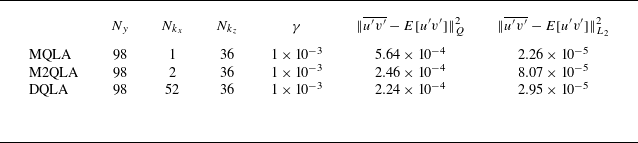


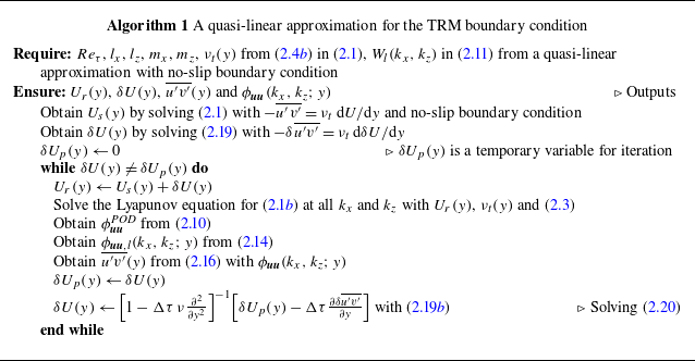
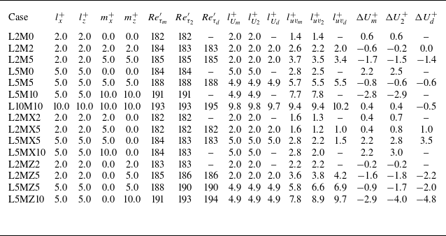


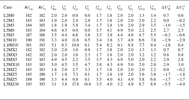


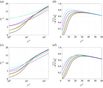

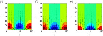


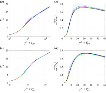


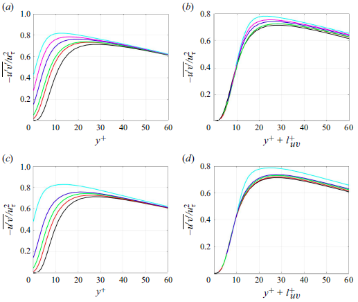


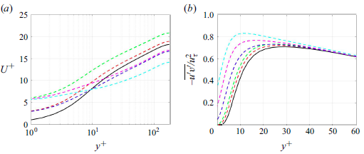

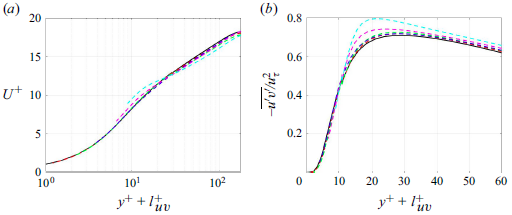


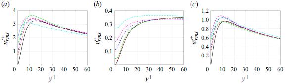

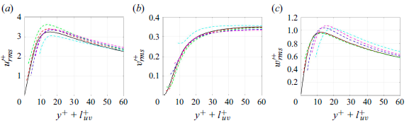


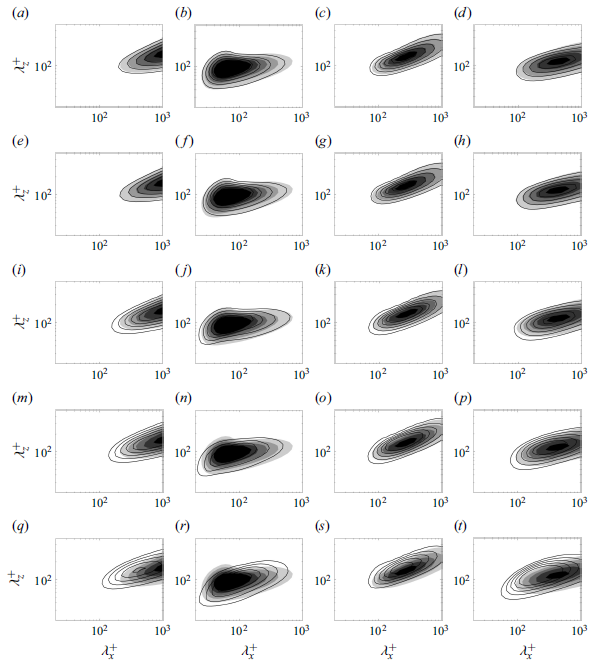


 Open access

