





1. Introduction
The motion of two immiscible fluids through a porous media is known to fall into different regimes, depending on the flow’s ability to mobilise trapped clusters (Avraam & Payatakes Reference Avraam and Payatakes1995). As such, the stability of trapped clusters is important for our basic understanding of two-phase porous-media flow in general and, hence, also for a long list of industrial applications. While enhanced oil recovery has traditionally dominated this list, many other important applications now also motivate the study of this problem; it is, for example, relevant to water or contaminant infiltration in soil, solute transport in unsaturated systems and soil remediation, and for discussions of these subjects, we refer the reader to the papers of Kirchner, Feng & Neal (Reference Kirchner, Feng and Neal2000), Zhan & Ng (Reference Zhan and Ng2004), Rahbeh & Mohtar (Reference Rahbeh and Mohtar2007) and Alamooti et al. (Reference Alamooti, Colombano, Glabe, Lion, Davarzani and Ahmadi-Sénichault2023). Naturally, the problem’s importance has led several authors to suggest solutions and, being based on mean-field arguments, these solutions not only improve our understanding, they also provide easy-to-use formulae for predicting whether a trapped cluster will be stable under given flow conditions. These formulae are, however, not always accurate and, since they are not derived from first principles, their range of validity is not known. In addition, as we will argue in the following, the existing mean-field arguments neglect several important features that become apparent when studying cluster stability on the pore scale.
Since the aim of this work is to study gravity-driven flows, we have chosen to base the following discussion on the Bond number, ${\textit{Bo}},$
rather than, e.g. the capillary number,
${\textit{Bo}},$
rather than, e.g. the capillary number, ${\textit{Ca}}$
. The Bond number measures the strength of the average pressure gradient (induced by gravity) relative to the surface tension between the two fluids and can hence be specified a priori in terms of the properties of the two fluids. In contrast, the capillary number measures the strength of the viscous stress between the two fluids relative to the surface tension and, as such, it cannot be predicted from the fluid properties, the reason being that there presently is no way of calculating the flow velocity (induced by gravity) from these parameters. An empirical relation between
${\textit{Ca}}$
. The Bond number measures the strength of the average pressure gradient (induced by gravity) relative to the surface tension between the two fluids and can hence be specified a priori in terms of the properties of the two fluids. In contrast, the capillary number measures the strength of the viscous stress between the two fluids relative to the surface tension and, as such, it cannot be predicted from the fluid properties, the reason being that there presently is no way of calculating the flow velocity (induced by gravity) from these parameters. An empirical relation between ${\textit{Bo}}$
and
${\textit{Bo}}$
and ${\textit{Ca}}$
, valid for the parameter values used in this work, is presented in the forthcoming § 4.2, enabling comparisons to the studies that characterise the flow in terms of the capillary number.
${\textit{Ca}}$
, valid for the parameter values used in this work, is presented in the forthcoming § 4.2, enabling comparisons to the studies that characterise the flow in terms of the capillary number.
A first step towards a characterisation of cluster stability was taken by Taber (Reference Taber1969), who experimentally showed that the fraction of trapped clusters that can be mobilised by a given flow is a function of the average pressure gradient divided by the surface tension between the two fluids. A few years later, Melrose & Brandner (Reference Melrose and Brandner1974) and Larson, Scriven & Davis (Reference Larson, Scriven and Davis1977) provided a mean-field argument suggesting that a trapped cluster cannot be stable if its size exceeds a numerical factor determined by the porous geometry times $r/{\textit{Bo}}$
, where
$r/{\textit{Bo}}$
, where $r$
corresponds to a typical pore size; exact definitions of
$r$
corresponds to a typical pore size; exact definitions of $r$
and
$r$
and ${\textit{Bo}}$
are given in § 2. Throughout this paper, we shall refer to this argument as MFA1 and we note that it was successfully applied by Tallakstad et al. (Reference Tallakstad, Løvoll, Knudsen, Ramstad, Flekkøy and Måløy2009a
) to explain the results of their measurements of cluster sizes in statistically steady flows. The argument first considers the pressure difference across the cluster and assumes that this quantity must equal the average pressure gradient times the size of the cluster. Second, based on the Young–Laplace equation, MFA1 assumes that the pressure difference that can be sustained by the trapped cluster is of the order of the surface tension divided by a typical pore size. Finally, equating the two pressure differences then gives the
${\textit{Bo}}$
are given in § 2. Throughout this paper, we shall refer to this argument as MFA1 and we note that it was successfully applied by Tallakstad et al. (Reference Tallakstad, Løvoll, Knudsen, Ramstad, Flekkøy and Måløy2009a
) to explain the results of their measurements of cluster sizes in statistically steady flows. The argument first considers the pressure difference across the cluster and assumes that this quantity must equal the average pressure gradient times the size of the cluster. Second, based on the Young–Laplace equation, MFA1 assumes that the pressure difference that can be sustained by the trapped cluster is of the order of the surface tension divided by a typical pore size. Finally, equating the two pressure differences then gives the $r/{\textit{Bo}}$
-dependence of the largest stable cluster size. While this argument is both simple and elegant, it however also neglects several important physical features of the problem. First of all, the assumption that a trapped cluster becomes unstable when the difference in pressure outside its most upstream (bottom) and downstream (top) openings exceeds the pressure difference that can be sustained by the average pore opening is questionable. The relative strength of two different cluster openings is determined by a competition between their widths as well as the inside and outside pressures to which the openings are exposed. As such, it is often not the opening located the furthest upstream that breaks first and, therefore, the relevant pressure difference is not necessarily the one between the bottom and the top. Moreover, the assumption disregards the fact that a large cluster is more likely to contain a wide (and therefore weak) opening than a small cluster and one would therefore expect this effect to contribute to the fact that large clusters, in general, are more easily mobilised than small clusters.
$r/{\textit{Bo}}$
-dependence of the largest stable cluster size. While this argument is both simple and elegant, it however also neglects several important physical features of the problem. First of all, the assumption that a trapped cluster becomes unstable when the difference in pressure outside its most upstream (bottom) and downstream (top) openings exceeds the pressure difference that can be sustained by the average pore opening is questionable. The relative strength of two different cluster openings is determined by a competition between their widths as well as the inside and outside pressures to which the openings are exposed. As such, it is often not the opening located the furthest upstream that breaks first and, therefore, the relevant pressure difference is not necessarily the one between the bottom and the top. Moreover, the assumption disregards the fact that a large cluster is more likely to contain a wide (and therefore weak) opening than a small cluster and one would therefore expect this effect to contribute to the fact that large clusters, in general, are more easily mobilised than small clusters.
The effect was described by Mathiesen et al. (Reference Mathiesen, Linga, Misztal, Renard and Le Borgne2023), who put forth an argument that we shall refer to as MFA2 in the remainder of this paper. This argument predicts that the largest stable cluster size should scale as $r/{\textit{Bo}}^{1/2}$
and, as such, it predicts more clusters to be unstable than MFA1, since mobilisation takes place for Bond numbers smaller than one. MFA2 differs from MFA1 by assuming that a cluster becomes unstable when its widest – and therefore weakest – opening can no longer sustain the pressure difference across the cluster. However, the maximum pressure difference that a random opening can withstand is assumed to follow an exponential distribution, and the
$r/{\textit{Bo}}^{1/2}$
and, as such, it predicts more clusters to be unstable than MFA1, since mobilisation takes place for Bond numbers smaller than one. MFA2 differs from MFA1 by assuming that a cluster becomes unstable when its widest – and therefore weakest – opening can no longer sustain the pressure difference across the cluster. However, the maximum pressure difference that a random opening can withstand is assumed to follow an exponential distribution, and the $r/{\textit{Bo}}^{1/2}$
-scaling turns out to be a result of the specific form of this distribution. Unfortunately, presently, no theoretical argument supports this specific form and, by assuming a different distribution, one may use the argument to predict that the largest stable cluster size should scale as
$r/{\textit{Bo}}^{1/2}$
-scaling turns out to be a result of the specific form of this distribution. Unfortunately, presently, no theoretical argument supports this specific form and, by assuming a different distribution, one may use the argument to predict that the largest stable cluster size should scale as $r/{\textit{Bo}}^\alpha$
for any desired value of
$r/{\textit{Bo}}^\alpha$
for any desired value of $\alpha$
. In addition, MFA2 suffers from other limitations, as it assumes that cluster openings can be considered independently and that the maximum pressure difference that an opening can sustain follows a simple universal distribution.
$\alpha$
. In addition, MFA2 suffers from other limitations, as it assumes that cluster openings can be considered independently and that the maximum pressure difference that an opening can sustain follows a simple universal distribution.
So far, we have described shortcomings that are specific to MFA1 and MFA2. A fundamental concern, which applies to any mean-field approach, is that the outside pressure field is necessarily approximated through the average pressure gradient of the flow. In other words, the random fluctuations of the pressure that appear on the pore scale are neglected. Since these fluctuations are mainly induced by the stochastic nature of the porous geometry, their typical size is roughly independent of the cluster size, implying that the fluctuation-to-mean ratio diverges in the limit where the cluster becomes small. As such, the mean-field approximation for the outside pressure can only be accurate for large clusters.
In summary, the stability of trapped clusters remains an open question; different scaling relations have been proposed, and their derivations are based on physical assumptions that do not universally hold and which do not take some key pore-scale mechanisms into account. The reason for this is, of course, the complicated, nonlinear nature of two-phase porous-media flow, which renders exact theoretical treatments very challenging and, at the same time, makes detailed experimental and numerical investigations both difficult and extremely time-consuming. However, for some specific applications, there exists analytical models succeeding in only taking the most relevant physical phenomena into account, allowing them to offer both accurate quantitative predictions as well as new physical insights. A prime example of this is the very simple stepwise fluid propagation model proposed by Cieplak & Robbins (Reference Cieplak and Robbins1988, Reference Cieplak and Robbins1990). Relying only on elementary geometric considerations, these authors showed that a cluster interface can become unstable in three different ways and by combining this with ‘a set of plausible rules’ for the formation of new interfaces following instability, as Singh et al. (Reference Singh, Jung, Brinkmann and Seemann2019) put it in their review, they managed to explain the role played by the contact angle during invasion processes. The validity of Cieplak & Robbins’ classification of the modes of instability has since been confirmed experimentally by Jung et al. (Reference Jung, Brinkmann, Seemann, Hiller, Sancez de la Lama and Herminghaus2016), and the recent work presented by, for example, Hu et al. (Reference Hu, Lan, Wei and Chen2019), Primkulov et al. (Reference Primkulov, Pahlavan, Fu, Zhao, MacMinn and Juanes2021) and Wang et al. (Reference Wang, Pereira, Sauret and Gan2023), is a testament to the fact that simple geometrical ideas continue to play an important role in two-phase porous media flow.
In this work, we consider a trapped cluster in a two-dimensional porous medium and develop a new, quasistatic model for studying its stability. While this model can also be derived for a three-dimensional system, we have chosen the two-dimensional setting because it allows us to highlight the model’s physical basis, which is easily overlooked in three-dimensional porous geometries. Since MFA1 and MFA2 apply equally well to two and three dimensions, the decision to consider a two-dimensional system is not a barrier to testing the validity of these arguments. Moreover, two-dimensional porous media are broadly used and represent an important reference in experiments, simulations and theory. The model consists of a set of coupled differential equations predicting how the geometry of the cluster changes with various parameters up to the point of breaking and we derive it by making geometrical considerations similar to those of Cieplak & Robbins (Reference Cieplak and Robbins1988), and by requiring mass conservation and that the cluster is in mechanical equilibrium at all times. As such, the derivation sheds new light on the fundamental understanding of cluster stability. Moreover, as the equations are much faster to solve than the full hydrodynamic problem, they provide a vehicle for exploring a much larger subset of the system’s parameter space than what is currently possible with direct numerical simulation. We use our model to show that the scaling laws for the largest stable cluster size predicted by the mean-field arguments MFA1 and MFA2 do not hold in general. Furthermore, we question the usefulness of expressing the largest stable cluster size on the form $r/{\textit{Bo}}^\alpha$
, where
$r/{\textit{Bo}}^\alpha$
, where $\alpha$
is some exponent; for as we will show, if one insists on this form,
$\alpha$
is some exponent; for as we will show, if one insists on this form, $\alpha$
is necessarily a complicated function of several different variables.
$\alpha$
is necessarily a complicated function of several different variables.
The remainder of this paper is laid out as follows. In § 2, we specify the porous-media system under consideration. In § 3, we develop the quasistatic model for predicting the evolution of the cluster geometry with respect to the Bond number and explain how to extract the point of breaking from this model. The model is validated against direct numerical simulations in § 4 and subsequently used to compute the probability that a cluster of a given size is stable as a function of the Bond number in § 5. Conclusions are drawn in § 6.
2. Physical system
We consider the stability of a single, trapped cluster of wetting (w) fluid surrounded by non-wetting (nw) fluid in a two-dimensional gravity-driven porous-media flow. We assume both fluids to be incompressible and immiscible, and we denote their dynamic viscosities by $\mu _{{w}}$
and
$\mu _{{w}}$
and $\mu _{{nw}}$
, and their mass densitites by
$\mu _{{nw}}$
, and their mass densitites by $\rho _{{w}}$
and
$\rho _{{w}}$
and $\rho _{{nw}}$
. The fluids are both subject to the gravitational acceleration
$\rho _{{nw}}$
. The fluids are both subject to the gravitational acceleration $\boldsymbol{g}$
, which we take to point in the positive
$\boldsymbol{g}$
, which we take to point in the positive $y$
-direction such that
$y$
-direction such that $\boldsymbol{g} = (0, g)$
. Moreover, we let
$\boldsymbol{g} = (0, g)$
. Moreover, we let $\gamma$
and
$\gamma$
and $\theta _0$
represent the surface tension between the fluids and the contact angle, respectively.
$\theta _0$
represent the surface tension between the fluids and the contact angle, respectively.
For the porous media, we consider idealised geometries consisting of square domains filled with non-overlapping, cylindrical obstacles of radius $r$
. Realisations of the geometries are generated using the random sequential adsorption procedure (see, for example, Feder Reference Feder1980), which is commonly used to construct random isotropic porous media with a single length scale. In this procedure, new obstacles are successively placed at random positions drawn from a uniform distribution over the domain such that the distance between any two obstacle centres is at least
$r$
. Realisations of the geometries are generated using the random sequential adsorption procedure (see, for example, Feder Reference Feder1980), which is commonly used to construct random isotropic porous media with a single length scale. In this procedure, new obstacles are successively placed at random positions drawn from a uniform distribution over the domain such that the distance between any two obstacle centres is at least $d_{\textit{min}} + 2r$
; the process terminates when this is no longer possible. Throughout this work, we use the value
$d_{\textit{min}} + 2r$
; the process terminates when this is no longer possible. Throughout this work, we use the value $d_{\textit{min}} = r/10$
for the minimum distance and we note that this implies that the porosity of the medium is close to
$d_{\textit{min}} = r/10$
for the minimum distance and we note that this implies that the porosity of the medium is close to $50 \,\%$
. Figure 1 shows a sketch of the system, including the trapped cluster and the streamlines of the flow.
$50 \,\%$
. Figure 1 shows a sketch of the system, including the trapped cluster and the streamlines of the flow.
A cluster of wetting fluid (red) surrounded by non-wetting fluid (blue) trapped between the cylindrical obstacles of the porous medium. The Bond number is smaller than the critical value such that the cluster lies still. In contrast, the non-wetting fluid flows according to a time-independent velocity field. The streamlines of the flow are illustrated by the yellow curves, which are actual streamlines taken from numerical simulations.

Figure 1. Long description
A diagram of a cluster of wetting fluid (red) surrounded by non-wetting fluid (blue) trapped between cylindrical obstacles in a porous medium. The Bond number is below the critical value, keeping the cluster stationary. The non-wetting fluid flows according to a time-independent velocity field, with streamlines illustrated by yellow curves representing actual streamlines from numerical simulations.
We fix the properties of the fluids and obstacles such that the flow around the trapped cluster is creeping and consider the stability of the cluster in terms of the Bond number
 \begin{align} {\textit{Bo}} \equiv \frac {\rho _{{w}} g r^2}{\gamma }. \end{align}
To be precise, we study the stability of trapped clusters in the following way: first, a circular drop of wetting fluid is released at a random position in the porous media. The Bond number is assumed to be so small that the drop quickly adheres to the surrounding obstacles and adjusts its geometry into a stable configuration. Second, the Bond number is increased very slowly, that is, over a time scale much longer than the time it takes the flow around the cluster to readjust to the new conditions. During this process, the cluster remains in mechanical equilibrium the entire time and the geometry of the cluster changes until an opening of the cluster finally becomes unstable and is pushed in. We call the Bond number where this happens the critical Bond number and denote it by ${\textit{Bo}}_{{crit}}$
. Therefore, it is important to realise that the instability of an opening does not necessarily lead to the cluster being mobilised. In some cases, the cluster is indeed mobilised, while in other cases, the cluster simply reconfigures into a different, stable geometry. The latter event may, for example, occur if obstacles are contained inside the trapped cluster. As such, one could also define the critical Bond number as the smallest value of
${\textit{Bo}}_{{crit}}$
. Therefore, it is important to realise that the instability of an opening does not necessarily lead to the cluster being mobilised. In some cases, the cluster is indeed mobilised, while in other cases, the cluster simply reconfigures into a different, stable geometry. The latter event may, for example, occur if obstacles are contained inside the trapped cluster. As such, one could also define the critical Bond number as the smallest value of ${\textit{Bo}}$
where the cluster is fully mobilised, i.e. completely pushed away from the region of space that it occupies in the limit
${\textit{Bo}}$
where the cluster is fully mobilised, i.e. completely pushed away from the region of space that it occupies in the limit ${\textit{Bo}} \rightarrow 0$
. This definition, however, easily becomes relatively involved and since it produces critical Bond numbers which are typically quite close to those corresponding to the first unstable opening (in particular, for small clusters), we have chosen to use the definition based on this criterion in this work.
${\textit{Bo}} \rightarrow 0$
. This definition, however, easily becomes relatively involved and since it produces critical Bond numbers which are typically quite close to those corresponding to the first unstable opening (in particular, for small clusters), we have chosen to use the definition based on this criterion in this work.
A cluster trapped between obstacles. The obstacles along the perimeter are labelled in counterclockwise direction and the centre of the $n$
th obstacle is at
$n$
th obstacle is at $\boldsymbol{r}_{\textit{obs},n}$
. Each pair of obstacle neighbours constitutes a cluster opening and is equipped with a local coordinate system,
$\boldsymbol{r}_{\textit{obs},n}$
. Each pair of obstacle neighbours constitutes a cluster opening and is equipped with a local coordinate system, $\{ \boldsymbol{\hat {t}}_n, \boldsymbol{\hat {n}}_n\}$
. The angle between
$\{ \boldsymbol{\hat {t}}_n, \boldsymbol{\hat {n}}_n\}$
. The angle between $\boldsymbol{\hat {t}}_n$
and the
$\boldsymbol{\hat {t}}_n$
and the $x$
-axis is denoted by
$x$
-axis is denoted by $\xi _n$
. The curve
$\xi _n$
. The curve $\mathcal{C}$
follows the circumference of the cluster and is oriented counterclockwise; for computational purposes, this curve is decomposed into segments along the fluid interfaces,
$\mathcal{C}$
follows the circumference of the cluster and is oriented counterclockwise; for computational purposes, this curve is decomposed into segments along the fluid interfaces, $\mathcal{C}_{\textit{int}, n}$
, and segments along the obstacles,
$\mathcal{C}_{\textit{int}, n}$
, and segments along the obstacles, $\mathcal{C}_{\textit{obs},n}$
.
$\mathcal{C}_{\textit{obs},n}$
.

Interface between the two fluids in the $n$
th opening of the cluster with obstacle locations
$n$
th opening of the cluster with obstacle locations $\boldsymbol{r}_{\textit{obs}, n}$
and
$\boldsymbol{r}_{\textit{obs}, n}$
and $\boldsymbol{r}_{\textit{obs}, n+1}$
, and local coordinate system
$\boldsymbol{r}_{\textit{obs}, n+1}$
, and local coordinate system $\{ \boldsymbol{\hat {t}}_n, \boldsymbol{\hat {n}}_n \}$
. The interface is assumed to be circular with radius
$\{ \boldsymbol{\hat {t}}_n, \boldsymbol{\hat {n}}_n \}$
. The interface is assumed to be circular with radius $R_n$
and centre
$R_n$
and centre $\boldsymbol{r}_{c, n}$
; the interface’s midpoint is denoted by
$\boldsymbol{r}_{c, n}$
; the interface’s midpoint is denoted by $\boldsymbol{r}_{\textit{int},n}$
. At the point of contact between the left obstacle and the interface, their tangent vectors are denoted by
$\boldsymbol{r}_{\textit{int},n}$
. At the point of contact between the left obstacle and the interface, their tangent vectors are denoted by $\boldsymbol{\hat {t}}_{\textit{obs},n}$
and
$\boldsymbol{\hat {t}}_{\textit{obs},n}$
and $\boldsymbol{\hat {t}}_{\textit{int},n}$
, respectively, and the angle between these vectors is the contact angle,
$\boldsymbol{\hat {t}}_{\textit{int},n}$
, respectively, and the angle between these vectors is the contact angle, $\theta _0$
. The angle
$\theta _0$
. The angle $\omega _n$
is measured positively upwards as the angle between
$\omega _n$
is measured positively upwards as the angle between $\boldsymbol{\hat {t}}_n$
and the line from the left obstacle’s centre to its point of contact with the interface; the angle
$\boldsymbol{\hat {t}}_n$
and the line from the left obstacle’s centre to its point of contact with the interface; the angle $\varOmega _n$
is measured positively upwards as the angle between
$\varOmega _n$
is measured positively upwards as the angle between $-\boldsymbol{\hat {t}}_n$
and the line from the interface’s centre to its point of intersection with the left obstacle. The inter-obstacle distance is denoted by
$-\boldsymbol{\hat {t}}_n$
and the line from the interface’s centre to its point of intersection with the left obstacle. The inter-obstacle distance is denoted by $d_n$
.
$d_n$
.

Figure 3. Long description
A diagram of the interface between two fluids in the opening of a cluster with obstacle locations and a local coordinate system. The interface is assumed to be circular with radius Rn and center rc,n. The interface’s midpoint is denoted by robs,n. At the point of contact between the left obstacle and the interface, their tangent vectors are denoted by n_hat_n and t_hat_n, respectively, and the angle between these vectors is the contact angle, theta_0. The angle omega_n is measured positively upwards as the angle between t_hat_n and the line from the left obstacle’s center to its point of contact with the interface. The angle theta_0 is measured positively upwards as the angle between n_hat_n and the line from the interface’s center to its point of intersection with the left obstacle. The inter-obstacle distance is denoted by d_n. The diagram also shows the positions of robs,n, robs,n+1, and rint,n.
3. A quasistatic model for predicting the critical Bond number
Consider the cluster shown in figure 2 and its $n$
th opening illustrated in figure 3. Under the assumptions that the interfaces between the two fluids are circular and infinitely thin, it turns out that the geometry of the cluster is completely determined by the inter-obstacle distances
$n$
th opening illustrated in figure 3. Under the assumptions that the interfaces between the two fluids are circular and infinitely thin, it turns out that the geometry of the cluster is completely determined by the inter-obstacle distances $\boldsymbol{d} = [d_1, d_2, \ldots , d_N]$
, the orientation angles
$\boldsymbol{d} = [d_1, d_2, \ldots , d_N]$
, the orientation angles $\boldsymbol{\xi } = [\xi _1, \xi _2, \ldots , \xi _N]$
and the opening angles
$\boldsymbol{\xi } = [\xi _1, \xi _2, \ldots , \xi _N]$
and the opening angles $\boldsymbol{\omega } = [\omega _1, \omega _2, \ldots , \omega _N ]$
, where
$\boldsymbol{\omega } = [\omega _1, \omega _2, \ldots , \omega _N ]$
, where $N$
is the number of cluster openings; figures 2 and 3 define the variables
$N$
is the number of cluster openings; figures 2 and 3 define the variables $d_n$
,
$d_n$
, $\xi _n$
and
$\xi _n$
and $\omega _n$
. Since both
$\omega _n$
. Since both $\boldsymbol{d}$
and
$\boldsymbol{d}$
and $\boldsymbol{\xi }$
are fixed quantities, any change in the cluster’s geometry can be described by a change in
$\boldsymbol{\xi }$
are fixed quantities, any change in the cluster’s geometry can be described by a change in $\boldsymbol{\omega }$
up to the point where an interface collapses and the cluster reconfigures its shape.
$\boldsymbol{\omega }$
up to the point where an interface collapses and the cluster reconfigures its shape.
The shape of the cluster changes with the Bond number and, in this section, we derive a simple, yet accurate model that predicts this change of shape. More specifically, we show that when all other parameters than the Bond number are held constant, $\boldsymbol{\omega }$
satisfies a system of coupled differential equations of the form
$\boldsymbol{\omega }$
satisfies a system of coupled differential equations of the form
 \begin{align} \unicode{x1D63C} \frac {\partial \boldsymbol{\omega }}{\partial ({\textit{Bo}})} = \boldsymbol{c}, \end{align}
where $\unicode{x1D63C}$
is a matrix of size
$\unicode{x1D63C}$
is a matrix of size $N \times N$
and
$N \times N$
and $\boldsymbol{c}$
is a vector of size
$\boldsymbol{c}$
is a vector of size $N$
. Since these quantities depend on
$N$
. Since these quantities depend on $\boldsymbol{\omega }$
in complicated, nonlinear ways, the system of equations cannot be solved analytically in general, but the time it takes to solve them numerically is substantially less than the time it would take to carry out corresponding simulations based on, for example, solving the Navier–Stokes equations for the two phases. In addition, and perhaps more importantly, the derivation of (3.1) provides insight into the physical mechanisms that govern the stability of the cluster; in fact, the equations are a consequence of requiring (1) that mass is conserved as
$\boldsymbol{\omega }$
in complicated, nonlinear ways, the system of equations cannot be solved analytically in general, but the time it takes to solve them numerically is substantially less than the time it would take to carry out corresponding simulations based on, for example, solving the Navier–Stokes equations for the two phases. In addition, and perhaps more importantly, the derivation of (3.1) provides insight into the physical mechanisms that govern the stability of the cluster; in fact, the equations are a consequence of requiring (1) that mass is conserved as ${\textit{Bo}}$
changes and (2) that the cluster is in mechanical equilibrium up to the point of breaking. We note that part (2) corresponds to the assumption that the Bond number is changed over a time scale which is much longer than the time the cluster needs to adjust itself to the new conditions. This is the reason why time does not play any role in (3.1) and the reason we call it quasistatic.
${\textit{Bo}}$
changes and (2) that the cluster is in mechanical equilibrium up to the point of breaking. We note that part (2) corresponds to the assumption that the Bond number is changed over a time scale which is much longer than the time the cluster needs to adjust itself to the new conditions. This is the reason why time does not play any role in (3.1) and the reason we call it quasistatic.
In what follows, we first show that the quantities $\boldsymbol{d}$
,
$\boldsymbol{d}$
, $\boldsymbol{\xi }$
and
$\boldsymbol{\xi }$
and $\boldsymbol{\omega }$
indeed determine the geometry of the cluster. Next, we calculate the area of the cluster; as we have assumed the fluids to be incompressible, mass conservation is equivalent to area conservation. We then derive a relation between the curvatures, vertical coordinates and pressures just outside two different cluster openings in mechanical equilibrium, which we use to establish (3.1). We then discuss the stability of a single opening and this naturally leads to a method for determining a cluster’s critical Bond number using this quasistatic model. Finally, we discuss how the change in cluster geometry can be predicted when other parameters than the Bond number are varied.
$\boldsymbol{\omega }$
indeed determine the geometry of the cluster. Next, we calculate the area of the cluster; as we have assumed the fluids to be incompressible, mass conservation is equivalent to area conservation. We then derive a relation between the curvatures, vertical coordinates and pressures just outside two different cluster openings in mechanical equilibrium, which we use to establish (3.1). We then discuss the stability of a single opening and this naturally leads to a method for determining a cluster’s critical Bond number using this quasistatic model. Finally, we discuss how the change in cluster geometry can be predicted when other parameters than the Bond number are varied.
3.1. Geometry of a trapped cluster
When describing a cluster’s geometry, it is convenient to label the obstacles along its perimeter in counterclockwise order as shown in figure 2, such that the $n$
th opening of the cluster lies between the
$n$
th opening of the cluster lies between the $n$
th and the
$n$
th and the $(n+1)$
th obstacle. We equip each opening with a local coordinate system
$(n+1)$
th obstacle. We equip each opening with a local coordinate system $\{ \boldsymbol{\hat {t}}_n, \boldsymbol{\hat {n}}_n \}$
, where
$\{ \boldsymbol{\hat {t}}_n, \boldsymbol{\hat {n}}_n \}$
, where $\boldsymbol{\hat {t}}_n$
is the unit vector pointing from the centre of the
$\boldsymbol{\hat {t}}_n$
is the unit vector pointing from the centre of the $n$
th obstacle,
$n$
th obstacle, $\boldsymbol{r}_{\textit{obs}, n}$
, towards the centre of the
$\boldsymbol{r}_{\textit{obs}, n}$
, towards the centre of the $(n+1)$
th obstacle,
$(n+1)$
th obstacle, $\boldsymbol{r}_{\textit{obs},n+1}$
, and
$\boldsymbol{r}_{\textit{obs},n+1}$
, and $\boldsymbol{\hat {n}}_n$
is found by rotating
$\boldsymbol{\hat {n}}_n$
is found by rotating $\boldsymbol{\hat {t}}_n$ $90^\circ$
counterclockwise. The orientation of the
$90^\circ$
counterclockwise. The orientation of the $n$
th local coordinate system relative to the global
$n$
th local coordinate system relative to the global $\{ \boldsymbol{\hat {x}}, \boldsymbol{\hat {y}}\}$
coordinate system is encoded in the orientation angle
$\{ \boldsymbol{\hat {x}}, \boldsymbol{\hat {y}}\}$
coordinate system is encoded in the orientation angle $\xi _n$
between the global
$\xi _n$
between the global $x$
-axis and
$x$
-axis and $\boldsymbol{\hat {t}}_n$
. We emphasise that all these quantities are independent of
$\boldsymbol{\hat {t}}_n$
. We emphasise that all these quantities are independent of ${\textit{Bo}}$
and can be calculated once and for all before solving (3.1).
${\textit{Bo}}$
and can be calculated once and for all before solving (3.1).
Now, assuming the fluid interfaces to be circular, each of them can be described by their radius, $R_n$
, and their centre,
$R_n$
, and their centre, $\boldsymbol{r}_{c,n}$
– see figure 3. Since a circular arc has constant curvature, we note that this assumption neglects the possibility that the pressure jump across the interface may in fact vary along the interface. This effect is expected to be largest for a cluster opening which is parallel to the mean flow direction, and for such an opening, one can show that the difference between the curvature at the bottom and the top of the interface is roughly proportional to the Bond number, the relative difference of the fluids’ densities as well as the width of the opening. As a consequence, the assumption of circular interfaces is only valid as long as the product of these quantities is small. One way of calculating the quantities
$\boldsymbol{r}_{c,n}$
– see figure 3. Since a circular arc has constant curvature, we note that this assumption neglects the possibility that the pressure jump across the interface may in fact vary along the interface. This effect is expected to be largest for a cluster opening which is parallel to the mean flow direction, and for such an opening, one can show that the difference between the curvature at the bottom and the top of the interface is roughly proportional to the Bond number, the relative difference of the fluids’ densities as well as the width of the opening. As a consequence, the assumption of circular interfaces is only valid as long as the product of these quantities is small. One way of calculating the quantities $R_n$
and
$R_n$
and $\boldsymbol{r}_{c,n}$
in terms of the opening angle
$\boldsymbol{r}_{c,n}$
in terms of the opening angle $\omega _n$
is to parametrise the curves along the circumference of the
$\omega _n$
is to parametrise the curves along the circumference of the $n$
th obstacle and the
$n$
th obstacle and the $n$
th interface; the two curves should intersect when the angles of the parametrisations are
$n$
th interface; the two curves should intersect when the angles of the parametrisations are $\omega _n$
and
$\omega _n$
and $\varOmega _n$
, respectively, and at the intersection point, the angle between the two curves should be the contact angle,
$\varOmega _n$
, respectively, and at the intersection point, the angle between the two curves should be the contact angle, $\theta _0$
. In the local coordinate system, a parametrisation of the circumference of the
$\theta _0$
. In the local coordinate system, a parametrisation of the circumference of the $n$
th obstacle is given by
$n$
th obstacle is given by
 \begin{align} \boldsymbol{r}(\omega ) = \boldsymbol{r}_{\textit{obs},n} + r \cos (\omega ) \boldsymbol{\hat {t}}_n + r \sin (\omega ) \boldsymbol{\hat {n}}_n, \end{align}
while the $n$
th fluid interface can be parametrised as
$n$
th fluid interface can be parametrised as
 \begin{align} \boldsymbol{r}(\varOmega ) = \boldsymbol{r}_{c,n} - R_n \cos (\varOmega ) \boldsymbol{\hat {t}}_n + R_n \sin (\varOmega ) \boldsymbol{\hat {n}}_n. \end{align}
We note that the obstacle parametrisation runs counterclockwise and that the interface parametrisation runs clockwise, in accordance with the signs of $\omega _n$
and
$\omega _n$
and $\varOmega _n$
defined in figure 3. The angle
$\varOmega _n$
defined in figure 3. The angle $\varOmega _n$
is found by requiring that the angle between the two curves’ tangent vectors
$\varOmega _n$
is found by requiring that the angle between the two curves’ tangent vectors $\boldsymbol{\hat {t}}_{\textit{obs},n}$
and
$\boldsymbol{\hat {t}}_{\textit{obs},n}$
and $\boldsymbol{\hat {t}}_{\textit{int},n}$
should equal the contact angle, and a straightforward calculation shows that
$\boldsymbol{\hat {t}}_{\textit{int},n}$
should equal the contact angle, and a straightforward calculation shows that
 \begin{align} \varOmega _n = \theta _0 - \omega _n. \end{align}
To calculate the radius of the fluid interface, we make use of the fact that all obstacles have the same radius. This implies that the centre of the interface must lie half-way between the obstacles, that is, on the perpendicular bisector of line connecting the two obstacle centres, and hence that $(\boldsymbol{r}_{c,n} - \boldsymbol{r}_{\textit{obs},n})\boldsymbol{\cdot }\boldsymbol{\hat {t}}_n = r + d_n/2$
. Equating (3.2) and (3.3) at the point where
$(\boldsymbol{r}_{c,n} - \boldsymbol{r}_{\textit{obs},n})\boldsymbol{\cdot }\boldsymbol{\hat {t}}_n = r + d_n/2$
. Equating (3.2) and (3.3) at the point where $\omega = \omega _n$
and
$\omega = \omega _n$
and $\varOmega = \varOmega _n$
, and taking the dot product with
$\varOmega = \varOmega _n$
, and taking the dot product with $\boldsymbol{\hat {t}}_n$
therefore implies that the normalised interface radius is given by the expression
$\boldsymbol{\hat {t}}_n$
therefore implies that the normalised interface radius is given by the expression
 \begin{align} \frac {R_n}{r} = \frac {d_n/r + 2\big ( 1 - \cos (\omega _n) \big ) }{2 \cos (\varOmega _n)}. \end{align}
The geometric description of the interface is completed by equating (3.2) and (3.3) at the intersection point and taking the dot product with $\boldsymbol{\hat {n}}_n$
; when combined with the above-mentioned symmetry argument, this operation yields
$\boldsymbol{\hat {n}}_n$
; when combined with the above-mentioned symmetry argument, this operation yields
 \begin{align} \frac {\boldsymbol{r}_{c,n}}{r} = \frac {\boldsymbol{r}_{\textit{obs},n}}{r} + \bigg (1 + \frac {d_n}{2 r} \bigg ) \boldsymbol{\hat {t}}_n - \bigg ( \frac {R_n}{r}\sin (\varOmega _n) - \sin (\omega _n) \bigg ) \boldsymbol{\hat {n}}_n. \end{align}
3.2. Area of a trapped cluster
To derive the area of a trapped cluster, we again consider the cluster depicted in figure 2. Using Green’s theorem, its area, $A_{\textit{cluster}}$
, can be calculated as the line integral
$A_{\textit{cluster}}$
, can be calculated as the line integral
 \begin{align} A_{\textit{cluster}} = \frac {1}{2} \oint _{\mathcal{C}} \big ( -y \, \mathrm{d} x + x \, \mathrm{d} y\big ), \end{align}
where $\mathcal{C}$
is the closed curve along the cluster’s circumference oriented counterclockwise. We note that the integral only equals the cluster area in the case where the cluster contains no embedded obstacles, that is, obstacles that are completely surrounded by wetting fluid, which may be present in the case of large clusters. However, since our only application of the cluster area is to make sure that it remains constant when the Bond number changes, the constant contributions to the area from embedded obstacles can be neglected for the present purpose. To make progress from here, we decompose
$\mathcal{C}$
is the closed curve along the cluster’s circumference oriented counterclockwise. We note that the integral only equals the cluster area in the case where the cluster contains no embedded obstacles, that is, obstacles that are completely surrounded by wetting fluid, which may be present in the case of large clusters. However, since our only application of the cluster area is to make sure that it remains constant when the Bond number changes, the constant contributions to the area from embedded obstacles can be neglected for the present purpose. To make progress from here, we decompose $\mathcal{C}$
into contributions from the fluid interfaces and the obstacles, as shown in figure 2, which gives that
$\mathcal{C}$
into contributions from the fluid interfaces and the obstacles, as shown in figure 2, which gives that
 \begin{align} A_{\textit{cluster}} = \frac {1}{2} \sum _{n = 1}^{N} \bigg ( \oint _{\mathcal{C}_{\textit{int},n}} \big ( -y \, \mathrm{d} x + x \, \mathrm{d} y \big ) + \oint _{\mathcal{C}_{\textit{obs},n}} \big ( -y \, \mathrm{d} x + x \, \mathrm{d} y \big ) \bigg ). \end{align}
To calculate the contribution from the $n$
th fluid interface, we employ the parametrisation (3.3) with
$n$
th fluid interface, we employ the parametrisation (3.3) with $\varOmega _n \leqslant \varOmega \leqslant \pi - \varOmega _n$
. Carrying out the integral (see Appendix A for a detailed derivation) yields
$\varOmega _n \leqslant \varOmega \leqslant \pi - \varOmega _n$
. Carrying out the integral (see Appendix A for a detailed derivation) yields
 \begin{align} \int _{\mathcal{C}_{\textit{int},n}} \big ( -y \, \mathrm{d} x + x \, \mathrm{d} y \big ) = - 2 R_n \cos \big (\varOmega _n \big ) \big ( \boldsymbol{r}_{\text{c},n} \boldsymbol{\cdot }\boldsymbol{\hat {n}}_n \big ) - R_n^2 \big ( \pi - 2\varOmega _n \big ). \end{align}
For the integral along the obstacle circumference, instead of using the local coordinate system, it turns out to be beneficial to use the global $\{ \boldsymbol{\hat {x}}, \boldsymbol{\hat {y}}\}$
-coordinate system to parametrise the curve segment. One possible choice is
$\{ \boldsymbol{\hat {x}}, \boldsymbol{\hat {y}}\}$
-coordinate system to parametrise the curve segment. One possible choice is
 \begin{align} \boldsymbol{r}(s) = \boldsymbol{r}_{\textit{obs},n} - r \cos (s) \boldsymbol{\hat {x}} + r \sin (s) \boldsymbol{\hat {y}}, \quad \text{where} \quad s_{1, n} \leqslant s \leqslant s_{2, n}, \end{align}
in which the upper limit of the parametrisation is $s_{2,n} = \pi - \xi _n - \omega _n$
, while the lower limit is
$s_{2,n} = \pi - \xi _n - \omega _n$
, while the lower limit is $s_{1,n} = 2\pi - \xi _{n-1} + \omega _{n-1}$
provided that this value is smaller than
$s_{1,n} = 2\pi - \xi _{n-1} + \omega _{n-1}$
provided that this value is smaller than $s_{2,n}$
; if it is larger than
$s_{2,n}$
; if it is larger than $s_{2,n}$
,
$s_{2,n}$
, $2\pi$
should be subtracted from
$2\pi$
should be subtracted from $s_{1,n}$
. This technicality only matters when evaluating the term
$s_{1,n}$
. This technicality only matters when evaluating the term $r^2 (s_{2,n} - s_{1,n})$
in (3.11), and we note that the subtraction of
$r^2 (s_{2,n} - s_{1,n})$
in (3.11), and we note that the subtraction of $2\pi$
is in fact irrelevant when establishing (3.1), since it disappears when differentiating with respect to
$2\pi$
is in fact irrelevant when establishing (3.1), since it disappears when differentiating with respect to ${\textit{Bo}}$
. Inserting the parametrisation (3.10) into the line integral, the contribution from the
${\textit{Bo}}$
. Inserting the parametrisation (3.10) into the line integral, the contribution from the $n$
th obstacle segment can be calculated in exactly the same way as the integral (3.9) and turns out to be
$n$
th obstacle segment can be calculated in exactly the same way as the integral (3.9) and turns out to be
 \begin{align} \begin{split} \int _{\mathcal{C}_{\textit{obs}},n} \big ( -y \, \mathrm{d} x + x \, \mathrm{d} y \big ) & = r y_{\textit{obs},n} \big ( \cos (s_{2,n}) - \cos (s_{1,n}) \big ) \\ & + r x_{\textit{obs},n} \big ( \sin (s_{2,n}) - \sin (s_{1,n}) \big ) \\ & - r^2 (s_{2,n} - s_{1,n}), \end{split} \end{align}
where $x_{\textit{obs},n}$
and
$x_{\textit{obs},n}$
and $y_{\textit{obs},n}$
are the
$y_{\textit{obs},n}$
are the $x$
- and
$x$
- and $y$
-coordinates of
$y$
-coordinates of $\boldsymbol{r}_{\textit{obs},n}$
, respectively. In combination, the results (3.8), (3.9) and (3.11) imply that the cluster area must satisfy the relation
$\boldsymbol{r}_{\textit{obs},n}$
, respectively. In combination, the results (3.8), (3.9) and (3.11) imply that the cluster area must satisfy the relation
 \begin{align} \begin{split} 2A_{\textit{cluster}}/r^2 = \sum _{n = 1}^{N} f_n (\omega _n, \omega _{n-1}), \end{split} \end{align}
in which the function $f_n(\omega _n, \omega _{n-1})$
is defined as
$f_n(\omega _n, \omega _{n-1})$
is defined as
 \begin{align} \begin{split} f_n(\omega _n, \omega _{n-1}) \equiv & - \frac {2 R_n}{r} \cos \big (\varOmega _n \big ) \big ( (\boldsymbol{r}_{c, n} / r) \boldsymbol{\cdot }\boldsymbol{n}_n \big ) - \bigg (\frac {R_n}{r} \bigg )^2 \big ( \pi - 2\varOmega _n \big ) \\ & + \frac {y_{\textit{obs},n}}{r} \big ( \cos (s_{2,n}) - \cos (s_{1,n}) \big ) \\ & + \frac {x_{\textit{obs},n}}{r} \big ( \sin (s_{2,n}) - \sin (s_{1,n}) \big ) \\ & - (s_{2,n} - s_{1,n}). \end{split} \end{align}
This completes the calculation of the cluster area.
3.3. Pressure difference across a trapped cluster
As long as a cluster is trapped, the pressure just outside its $n$
th opening is related to the pressure just outside its
$n$
th opening is related to the pressure just outside its $i$
th opening. To show this, we first define the outer and inner points of the
$i$
th opening. To show this, we first define the outer and inner points of the $n$
th fluid interface as
$n$
th fluid interface as $\boldsymbol{r}_{\textit{out},n} \equiv \boldsymbol{r}_{\textit{int},n} - \delta \boldsymbol{\hat {n}}_n$
and
$\boldsymbol{r}_{\textit{out},n} \equiv \boldsymbol{r}_{\textit{int},n} - \delta \boldsymbol{\hat {n}}_n$
and $\boldsymbol{r}_{\textit{in},n} \equiv \boldsymbol{r}_{\textit{int},n} + \delta \boldsymbol{\hat {n}}_n$
, and equivalently for the
$\boldsymbol{r}_{\textit{in},n} \equiv \boldsymbol{r}_{\textit{int},n} + \delta \boldsymbol{\hat {n}}_n$
, and equivalently for the $i$
th interface. Here,
$i$
th interface. Here, $\boldsymbol{r}_{\textit{int},n} \equiv \boldsymbol{r}_{c,n} + R_n \boldsymbol{\hat {n}}_n$
is the midpoint of the
$\boldsymbol{r}_{\textit{int},n} \equiv \boldsymbol{r}_{c,n} + R_n \boldsymbol{\hat {n}}_n$
is the midpoint of the $n$
th interface as illustrated in figure 3, and
$n$
th interface as illustrated in figure 3, and $\delta$
is a length scale which is very large relative to the width of the interface and very small relative to the obstacle radius. Next, we consider the momentum balance across the
$\delta$
is a length scale which is very large relative to the width of the interface and very small relative to the obstacle radius. Next, we consider the momentum balance across the $n$
th interface, which requires that the equation
$n$
th interface, which requires that the equation
 \begin{align} \begin{split} \big ( p_{\textit{out},n} - p_{{in}, n} \big ) \boldsymbol{\hat {n}}_n = & \gamma \kappa _n \boldsymbol{\hat {n}}_n + \mu _{{nw}} \Big (\boldsymbol{\nabla }\boldsymbol{u}_{\textit{out},n} + (\boldsymbol{\nabla }\boldsymbol{u}_{\textit{out},n})^\top \Big ) \boldsymbol{\hat {n}}_n \\ & - \mu _{{w}} \Big (\boldsymbol{\nabla }\boldsymbol{u}_{\textit{in},n} + (\boldsymbol{\nabla }\boldsymbol{u}_{\textit{in},n})^\top \Big ) \boldsymbol{\hat {n}}_n \end{split} \end{align}
is satisfied (see e.g. the derivation in § 1.1.2 of the book by Gross & Reusken Reference Gross and Reusken2011). In this equation, $\kappa _n \equiv 1/R_n$
is the curvature of the
$\kappa _n \equiv 1/R_n$
is the curvature of the $n$
th interface,
$n$
th interface, $\boldsymbol{u}$
is the velocity field, and the subscripts ‘out,
$\boldsymbol{u}$
is the velocity field, and the subscripts ‘out, $n$
’ and ‘in,
$n$
’ and ‘in, $n$
’ signify that the sub-scripted quantity is evaluated at
$n$
’ signify that the sub-scripted quantity is evaluated at $\boldsymbol{r}_{{out}, n}$
and
$\boldsymbol{r}_{{out}, n}$
and $\boldsymbol{r}_{{in}, n}$
, respectively. Since
$\boldsymbol{r}_{{in}, n}$
, respectively. Since $\boldsymbol{u}$
is continuous across the interface, we note that the fluid inside the trapped cluster may in fact circulate. From the simulations presented in §§ 4 and 5, we have, however, found that the fluid velocity and its gradient inside the trapped cluster are always very small relative to the corresponding quantities of the outside flow, and for that reason, we neglect the last term on the right-hand side of (3.14). Interestingly, this implies that the viscosity of the wetting fluid does not impact the stability of the cluster and, as a consequence, that the ratio of the two fluids’ viscosities cannot be a relevant parameter for cluster stability (provided, as in this case, that substantial circulation inside the cluster can be ruled out). In addition, a crude order-of-magnitude estimate shows that
$\boldsymbol{u}$
is continuous across the interface, we note that the fluid inside the trapped cluster may in fact circulate. From the simulations presented in §§ 4 and 5, we have, however, found that the fluid velocity and its gradient inside the trapped cluster are always very small relative to the corresponding quantities of the outside flow, and for that reason, we neglect the last term on the right-hand side of (3.14). Interestingly, this implies that the viscosity of the wetting fluid does not impact the stability of the cluster and, as a consequence, that the ratio of the two fluids’ viscosities cannot be a relevant parameter for cluster stability (provided, as in this case, that substantial circulation inside the cluster can be ruled out). In addition, a crude order-of-magnitude estimate shows that $\mu _{{nw}} |\boldsymbol{\nabla }\boldsymbol{u}_{\textit{out},n} | /(\gamma \kappa _n) = O({\textit{Ca}})$
, where
$\mu _{{nw}} |\boldsymbol{\nabla }\boldsymbol{u}_{\textit{out},n} | /(\gamma \kappa _n) = O({\textit{Ca}})$
, where ${\textit{Ca}} \equiv \mu _{{nw}} v_0 / \gamma$
is the capillary number of the flow in the non-wetting fluid and
${\textit{Ca}} \equiv \mu _{{nw}} v_0 / \gamma$
is the capillary number of the flow in the non-wetting fluid and $v_0$
is a typical velocity of the flow. Hence, as long as the capillary number is small, the second term on the right-hand side of (3.14) can be neglected and the pressure differences across the
$v_0$
is a typical velocity of the flow. Hence, as long as the capillary number is small, the second term on the right-hand side of (3.14) can be neglected and the pressure differences across the $n$
th and
$n$
th and $i$
th interfaces are given by the well-known Young–Laplace equation, i.e.
$i$
th interfaces are given by the well-known Young–Laplace equation, i.e.
 \begin{align} \left \{ \begin{aligned} p_{\textit{out},n} - p_{\textit{in},n} & = \kappa _n \gamma , \\[3pt] p_{\textit{out},i} - p_{\textit{in},i} & = \kappa _i \gamma . \end{aligned} \right . \end{align}
As is evident from these equations, we choose the curvature to be positive when the pressure on the outside is larger than on the inside, that is, $\kappa _n$
is positive whenever the non-wetting side of the interface is convex. The final step in relating
$\kappa _n$
is positive whenever the non-wetting side of the interface is convex. The final step in relating $p_{\textit{out},n}$
to
$p_{\textit{out},n}$
to $p_{\textit{out},i}$
consists in noting that the pressure inside the trapped cluster must be hydrostatic; the contribution from viscous effects to the pressure difference is insignificant because the fluid – to a very good approximation – lies still there and, hence,
$p_{\textit{out},i}$
consists in noting that the pressure inside the trapped cluster must be hydrostatic; the contribution from viscous effects to the pressure difference is insignificant because the fluid – to a very good approximation – lies still there and, hence,
 \begin{align} p_{\textit{in},n} - p_{\textit{in},i} = \rho _{{w}} g (y_{\textit{int}, n} - y_{\textit{int,i}}), \end{align}
and if we subtract the two equations in (3.15), use (3.16) to eliminate the pressure difference inside the cluster and normalise by $\rho _{{w}} g r$
, we find that
$\rho _{{w}} g r$
, we find that
 \begin{align} \frac {p_{\textit{out},n} - p_{\textit{out},i}}{\rho _{{w}} g r} = \frac {\kappa _n r - \kappa _i r}{{\textit{Bo}}} + \frac {y_{\textit{int},n} - y_{\textit{int},i}}{r}. \end{align}
At a first glance, one would think that this relation imposes $N (N - 1)/2$
constraints on the geometry of the cluster, because it should hold for all possible combinations of
$N (N - 1)/2$
constraints on the geometry of the cluster, because it should hold for all possible combinations of $n$
and
$n$
and $i$
. However, if it holds for
$i$
. However, if it holds for $i = 1$
and all
$i = 1$
and all $n \geqslant 2$
, then the relation is automatically satisfied for all possible choices of
$n \geqslant 2$
, then the relation is automatically satisfied for all possible choices of $n$
and
$n$
and $i$
. This is implied by the linearity of the relation. As such, (3.17) only imposes
$i$
. This is implied by the linearity of the relation. As such, (3.17) only imposes $N-1$
constraints on the cluster geometry.
$N-1$
constraints on the cluster geometry.
In what follows, we will assume that the left-hand side of (3.17) is independent of the Bond number. As we envision changing the Bond number by varying either $g$
or
$g$
or $\gamma$
, this is reasonable when recalling that a creeping flow is accurately described by the Stokes equation and therefore linear in the driving force and otherwise determined by the geometry. Since the pressure difference is normalised by
$\gamma$
, this is reasonable when recalling that a creeping flow is accurately described by the Stokes equation and therefore linear in the driving force and otherwise determined by the geometry. Since the pressure difference is normalised by $g$
, changing the value of this parameter does not have a direct effect on the left-hand side. Moreover, as we only consider the range
$g$
, changing the value of this parameter does not have a direct effect on the left-hand side. Moreover, as we only consider the range ${\textit{Bo}} \leqslant {\textit{Bo}}_{{crit}}$
, the changes in the cluster geometry are necessarily small. In particular, no pathways for the non-wetting fluid are created nor destroyed in this range. As such, the geometrical contribution to the change in the normalised pressure difference is expected to be small, which it indeed is. Figure 4 shows an example of this by comparing a trapped clusters in two different states in which it is either very far or very close to breaking. The validation of the quasistatic model against numerical simulations in § 4 provides further evidence that the assumption is indeed satisfied to a good approximation.
${\textit{Bo}} \leqslant {\textit{Bo}}_{{crit}}$
, the changes in the cluster geometry are necessarily small. In particular, no pathways for the non-wetting fluid are created nor destroyed in this range. As such, the geometrical contribution to the change in the normalised pressure difference is expected to be small, which it indeed is. Figure 4 shows an example of this by comparing a trapped clusters in two different states in which it is either very far or very close to breaking. The validation of the quasistatic model against numerical simulations in § 4 provides further evidence that the assumption is indeed satisfied to a good approximation.
Normalised pressure field around a trapped cluster for ${\textit{Bo}} = 0.025$
and
${\textit{Bo}} = 0.025$
and ${\textit{Bo}} = 0.125$
, corresponding to capillary numbers
${\textit{Bo}} = 0.125$
, corresponding to capillary numbers ${\textit{Ca}} = 0.00025$
and
${\textit{Ca}} = 0.00025$
and ${\textit{Ca}} = 0.00125$
, respectively. In the two cases, the cluster is either very far (panel a) of very close (panel b) to breaking, yet the pressure fields around the cluster are essentially the same. The pressure inside the cluster is larger in the small-
${\textit{Ca}} = 0.00125$
, respectively. In the two cases, the cluster is either very far (panel a) of very close (panel b) to breaking, yet the pressure fields around the cluster are essentially the same. The pressure inside the cluster is larger in the small- ${\textit{Bo}}$
case than in the large-
${\textit{Bo}}$
case than in the large- ${\textit{Bo}}$
case, because the Bond number is varied by varying the surface tension, while keeping the gravitational acceleration constant. The pressure field is calculated using the DNS model described in § 4.1 using a circular cluster with radius
${\textit{Bo}}$
case, because the Bond number is varied by varying the surface tension, while keeping the gravitational acceleration constant. The pressure field is calculated using the DNS model described in § 4.1 using a circular cluster with radius $r_{{circle}}/r = 4$
as the initial condition.
$r_{{circle}}/r = 4$
as the initial condition.

3.4. System of differential equations governing the cluster geometry
Equations (3.12) and (3.17) govern the geometry of the cluster as the Bond number changes. As we have shown, all geometric changes are ultimately determined by changes in the opening angles, $\boldsymbol{\omega } = [\omega _1, \omega _2, \ldots , \omega _N]$
, which in turn depend on a long list of parameters. However, as we are presently only concerned with changes in the opening angles induced by changes in
$\boldsymbol{\omega } = [\omega _1, \omega _2, \ldots , \omega _N]$
, which in turn depend on a long list of parameters. However, as we are presently only concerned with changes in the opening angles induced by changes in ${\textit{Bo}}$
, we consider
${\textit{Bo}}$
, we consider $\omega _n$
a function of this variable only. Hence, if we require the mass of the cluster to be independent of the Bond number, taking the derivative of (3.12) with respect to
$\omega _n$
a function of this variable only. Hence, if we require the mass of the cluster to be independent of the Bond number, taking the derivative of (3.12) with respect to ${\textit{Bo}}$
, yields
${\textit{Bo}}$
, yields
 \begin{align} 0 = \sum _{n = 1}^{N} \bigg ( \frac {\partial f_n}{\partial \omega _n} + \frac {\partial f_{n+1}}{\partial \omega _n} \bigg ) \frac {\partial \omega _n}{\partial ({\textit{Bo}})}. \end{align}
Here, periodic indexing is employed such that $f_{N+1}(\omega _{N+1}, \omega _{N}) = f_1(\omega _1, \omega _{N})$
. This is the first of the
$f_{N+1}(\omega _{N+1}, \omega _{N}) = f_1(\omega _1, \omega _{N})$
. This is the first of the $N$
equations that constitute (3.1); the remaining
$N$
equations that constitute (3.1); the remaining $N-1$
equations are derived from the relation (3.17). Setting
$N-1$
equations are derived from the relation (3.17). Setting $i = 1$
and making the assumption that the left-hand side is independent of the Bond number, taking the derivative with respect to
$i = 1$
and making the assumption that the left-hand side is independent of the Bond number, taking the derivative with respect to ${\textit{Bo}}$
yields
${\textit{Bo}}$
yields
 \begin{align} \begin{split} 0 & = \frac {\mathrm{d}}{\mathrm{d} ({\textit{Bo}})} \bigg ( \frac {p_{\textit{out},n} - p_{\textit{out},1}}{\rho _{{w}} g r} \bigg ) \\[5pt] & = \frac {\mathrm{d}}{\mathrm{d} ({\textit{Bo}})} \bigg ( \frac {\kappa _n r - \kappa _1 r}{{\textit{Bo}}} + \frac {y_{\textit{int},n} - y_{\textit{int},1}}{r} \bigg ) \\[5pt] & = \frac {1}{{\textit{Bo}}} \frac {\mathrm{d} (\kappa _n r)}{\mathrm{d} {\textit{Bo}}} - \frac {1}{{\textit{Bo}}} \frac {\mathrm{d} (\kappa _1 r)}{\mathrm{d} {\textit{Bo}}} - \frac {\kappa _n r - \kappa _1 r}{{\textit{Bo}}^2} + \frac {\mathrm{d} (y_{\textit{int},n}/r)}{\mathrm{d} ({\textit{Bo}})} - \frac {\mathrm{d} (y_{\textit{int},1}/r)}{\mathrm{d} ({\textit{Bo}})} \end{split} \end{align}
for $n = 2, 3, \ldots , N$
. Rearranging terms then leads to the equation
$n = 2, 3, \ldots , N$
. Rearranging terms then leads to the equation
 \begin{align} \bigg ( \frac {\mathrm{d} (y_{\textit{int},1}/r)}{\mathrm{d} \omega _1} + \frac {1}{{\textit{Bo}}} \frac {\mathrm{d} (\kappa _1 r)}{\mathrm{d} \omega _1} \bigg ) \frac {\partial \omega _1}{\partial ({\textit{Bo}})} - \bigg ( \frac {\mathrm{d} (y_{\textit{int},n}/r)}{\mathrm{d} \omega _n} + \frac {1}{{\textit{Bo}}} \frac {\mathrm{d} (\kappa _n r)}{\mathrm{d} \omega _n} \bigg ) \frac {\partial \omega _n}{\partial ({\textit{Bo}})} = \frac {\kappa _1 r - \kappa _n r}{({\textit{Bo}})^2}, \end{align}
which, in combination with (3.18), constitutes the system of $N$
coupled equations (3.1) governing the evolution of the opening angles as a function of the Bond number. To arrive at the matrix formulation (3.1), we simply define
$N$
coupled equations (3.1) governing the evolution of the opening angles as a function of the Bond number. To arrive at the matrix formulation (3.1), we simply define
 \begin{align} a_n & \equiv \frac {\partial f_n}{\partial \omega _n} + \frac {\partial f_{n+1}}{\partial \omega _n}, \\[-12pt]\nonumber \end{align}
 \begin{align} b_n & \equiv \frac {\mathrm{d} (y_{\textit{int},n}/r)}{\mathrm{d} \omega _n} + \frac {1}{{\textit{Bo}}}\frac {\mathrm{d} (\kappa _n r)}{\mathrm{d} \omega _n}, \\[-12pt]\nonumber \end{align}
 \begin{align} c_n & \equiv \frac {\kappa _1 r - \kappa _n r }{({\textit{Bo}})^2}, \end{align}
and set the matrix $\unicode{x1D63C}$
and vector
$\unicode{x1D63C}$
and vector $\boldsymbol{c}$
to
$\boldsymbol{c}$
to
 \begin{align}\unicode{x1D63C} = \begin{bmatrix} a_1 & a_2 & a_3 & {\cdots} & a_{N-1} & a_{N} \\[3pt] b_1 & -b_2 & 0 & {\cdots} & 0 & 0 \\[3pt] b_1 & 0 & -b_3 & {\cdots} & 0 & 0 \\[3pt] \vdots & \vdots & \vdots & \ddots & \vdots & \vdots \\[3pt] b_1 & 0 & 0 & {\cdots} & -b_{N-1} & 0 \\[3pt] b_1 & 0 & 0 & {\cdots} & 0 & -b_{N} \\ \end{bmatrix} \!, \quad \boldsymbol{c} = \begin{bmatrix} 0 \\[3pt] c_2 \\[3pt] c_3 \\[3pt] \vdots \\[3pt] c_{N-1} \\[3pt] c_{N} \end{bmatrix}\!. \end{align}
Given an initial configuration, $(\boldsymbol{\omega }_0, {\textit{Bo}}_0)$
, the set of equations (3.1) is easily integrated numerically with respect to the Bond number by any standard ordinary differential equation solver. As such, it only remains for us to clarify up to which Bond number one should integrate to predict the point of breaking. This is done in the following.
$(\boldsymbol{\omega }_0, {\textit{Bo}}_0)$
, the set of equations (3.1) is easily integrated numerically with respect to the Bond number by any standard ordinary differential equation solver. As such, it only remains for us to clarify up to which Bond number one should integrate to predict the point of breaking. This is done in the following.
3.5. When does a cluster become unstable?
As long as the Bond number is smaller than its critical value, the interfaces of the cluster can balance out the pressure difference across them by adjusting their shapes. More precisely, if the pressure difference across the $n$
th interface is
$n$
th interface is $\Delta p_n$
, then the interface will adjust its curvature such that the Young–Laplace equation is satisfied. Using the expression (3.5) for the radius of the interface, the expression (3.4) for the angle
$\Delta p_n$
, then the interface will adjust its curvature such that the Young–Laplace equation is satisfied. Using the expression (3.5) for the radius of the interface, the expression (3.4) for the angle $\varOmega _n$
and normalising by
$\varOmega _n$
and normalising by $\rho _{{w}} g r$
, the Young–Laplace equation can be written as
$\rho _{{w}} g r$
, the Young–Laplace equation can be written as
 \begin{align} \frac {\Delta p_n}{\rho _{{w}} g r} = \frac {1}{{\textit{Bo}}} \, \frac {2 \cos (\theta _0 - \omega _n)}{d_n/r + 2\big ( 1 - \cos (\omega _n) \big )}. \end{align}
This is the (normalised) pressure difference that the $n$
th interface can sustain by opening up to the angle
$n$
th interface can sustain by opening up to the angle $\omega _n$
. Plots of this pressure difference as a function of
$\omega _n$
. Plots of this pressure difference as a function of $\omega _n$
are shown in figure 5 for
$\omega _n$
are shown in figure 5 for $\theta _0 = \pi /3$
for different values of
$\theta _0 = \pi /3$
for different values of $d_n/r$
, and from this, it is clear that the pressure difference has a global maximum. One may interpret this result in the following way: if the cluster is initially stable, it can respond to an increasing pressure on its outer side, a decreasing pressure on its inner side or a weakening of the surface tension by moving inwards. Since the contact angle is constant, the new position further inwards will ensure that the curvature of the interface is larger and, therefore, that the interface becomes stronger. This, however, only works up to a certain critical angle, which we denote by
$d_n/r$
, and from this, it is clear that the pressure difference has a global maximum. One may interpret this result in the following way: if the cluster is initially stable, it can respond to an increasing pressure on its outer side, a decreasing pressure on its inner side or a weakening of the surface tension by moving inwards. Since the contact angle is constant, the new position further inwards will ensure that the curvature of the interface is larger and, therefore, that the interface becomes stronger. This, however, only works up to a certain critical angle, which we denote by $\omega _{\textit{crit},n}$
. Beyond this angle, further inwards movement will result in a smaller curvature and hence a weakening of the interface. Differentiating (3.23) with respect to
$\omega _{\textit{crit},n}$
. Beyond this angle, further inwards movement will result in a smaller curvature and hence a weakening of the interface. Differentiating (3.23) with respect to $\omega _n$
, it is straightforward to show that the critical angle is given by the expression
$\omega _n$
, it is straightforward to show that the critical angle is given by the expression
 \begin{align} \omega _{\textit{crit},n} = \theta _0 - \sin ^{-1} \bigg ( \frac {2 \sin (\theta _0)}{d_n/r + 2} \bigg ). \end{align}
When the flow conditions are such that one of the cluster’s openings is pushed to its critical value, the cluster becomes unstable. If some small perturbation pushes this interface just a tiny bit further in, it will become weaker and therefore keep yielding to the outside pressure until it finally collapses. The critical value of the Bond number for a given cluster can thus be computed by solving (3.1) up to the point where $\omega _n = \omega _{\textit{crit},n}$
for some
$\omega _n = \omega _{\textit{crit},n}$
for some $n$
.
$n$
.
We note that this instability is the well-known Haines jump, discovered by Haines (Reference Haines1930) now nearly a century ago. Cieplak & Robbins (Reference Cieplak and Robbins1988) refer to this event as a ‘burst’ and, as they have shown, there are other ways in which an interface can be unstable. For example, an interface may split into two new interfaces if it touches another obstacle before reaching its critical angle. The detection of such an event could, in principle, be built into the numerical solution of the model proposed here. We have, however, not done so because the continuation after the touch would most likely require a full (highly expensive) recomputation of the outside pressure field. While the small movements of an interface do not lead to large changes in the surrounding pressure, a reconfiguration of the interfaces oftentimes does. For small clusters, we note that this simplification does not affect the computation of ${\textit{Bo}}_{{crit}}$
, because these do not have any embedded obstacles such that a touching event could take place. For large clusters, however, we acknowledge that the simplification may add to the uncertainty of the computed values of
${\textit{Bo}}_{{crit}}$
, because these do not have any embedded obstacles such that a touching event could take place. For large clusters, however, we acknowledge that the simplification may add to the uncertainty of the computed values of ${\textit{Bo}}_{{crit}}$
.
${\textit{Bo}}_{{crit}}$
.
Pressure difference across the $n$
th cluster opening given by (3.23) as a function of the angle
$n$
th cluster opening given by (3.23) as a function of the angle $\omega _n$
for
$\omega _n$
for $\theta = \pi /3$
and different values of the non-dimensional inter-obstacle distance
$\theta = \pi /3$
and different values of the non-dimensional inter-obstacle distance $d_n/r$
.
$d_n/r$
.

3.6. Varying other parameters than the Bond number
The Bond number is not the only parameter on which the trapped cluster’s geometry depends; for example, it also depends on the ratio of fluid densities, $\rho _{{w}}/\rho _{{nw}}$
, and the contact angle,
$\rho _{{w}}/\rho _{{nw}}$
, and the contact angle, $\theta _0$
, and using an approach similar to that mentioned earlier, it is possible to derive equations corresponding to (3.1) for predicting the change in
$\theta _0$
, and using an approach similar to that mentioned earlier, it is possible to derive equations corresponding to (3.1) for predicting the change in $\boldsymbol{\omega }$
when these parameters are varied. In Appendix B, we show and validate that when the ratio
$\boldsymbol{\omega }$
when these parameters are varied. In Appendix B, we show and validate that when the ratio $\rho _{{w}}/\rho _{{nw}}$
is varied while keeping all other variables fixed, the opening angles satisfy the system of equations
$\rho _{{w}}/\rho _{{nw}}$
is varied while keeping all other variables fixed, the opening angles satisfy the system of equations
 \begin{align}\unicode{x1D63C} \frac {\partial \boldsymbol{\omega }}{\partial \left(\frac {\rho _{{w}}}{\rho _{{nw}}}\right)} = \boldsymbol{c}_{\rho _{{w}}/\rho _{{nw}}}, \end{align}
in which $\unicode{x1D63C}$
is the same as in (3.1) and
$\unicode{x1D63C}$
is the same as in (3.1) and $\boldsymbol{c}_{\rho _{{w}}/\rho _{{nw}}}$
is given by (B3). We note that this set of equations allows for cost-efficient computation of the critical Bond number as a function of the density ratio. Given a cluster geometry for particular values of
$\boldsymbol{c}_{\rho _{{w}}/\rho _{{nw}}}$
is given by (B3). We note that this set of equations allows for cost-efficient computation of the critical Bond number as a function of the density ratio. Given a cluster geometry for particular values of ${\textit{Bo}}$
and
${\textit{Bo}}$
and $\rho _{{w}}/\rho _{{nw}}$
, one can first integrate
$\rho _{{w}}/\rho _{{nw}}$
, one can first integrate $\boldsymbol{\omega }$
with respect to the density ratio up to the desired value using (3.25) before computing
$\boldsymbol{\omega }$
with respect to the density ratio up to the desired value using (3.25) before computing ${\textit{Bo}}_{{crit}}$
using (3.1). A set of equations that allows for changes in
${\textit{Bo}}_{{crit}}$
using (3.1). A set of equations that allows for changes in $\theta _0$
can likewise be derived, but we have not done so in the present work. A quasistatic model for the change in cluster geometry with respect to the parameters of the porous geometry can, however, not be derived. Studying how
$\theta _0$
can likewise be derived, but we have not done so in the present work. A quasistatic model for the change in cluster geometry with respect to the parameters of the porous geometry can, however, not be derived. Studying how ${\textit{Bo}}_{{crit}}$
depends on, say, the minimum required distance between two obstacles would require completely new initial conditions for the trapped cluster geometries.
${\textit{Bo}}_{{crit}}$
depends on, say, the minimum required distance between two obstacles would require completely new initial conditions for the trapped cluster geometries.
At this point, a comment on computational efficiency is appropriate, as we have repeatedly asserted that the quasistatic model is significantly faster than direct numerical simulations for predicting the critical Bond number. This claim may appear counterintuitive, given that the quasistatic model currently requires an initial condition that can only be obtained through a direct simulation. The key advantage, however, lies in the fact that only a single expensive simulation per cluster is needed to compute the critical Bond number as a function of the density ratio and, potentially, the contact angle. In contrast, without the quasistatic model, 5–10 direct simulations would be required for each combination of density ratio and contact angle. For a single pair of the density ratio and the contact angle, the speed-up is therefore roughly 5–10 times, while, if a detailed study across $(\rho _{{w}}/\rho _{nw}, \theta _0)$
-space was to be carried out, it is fair to say that employing the quasistatic model would lead to computational savings of several orders of magnitude.
$(\rho _{{w}}/\rho _{nw}, \theta _0)$
-space was to be carried out, it is fair to say that employing the quasistatic model would lead to computational savings of several orders of magnitude.
In this connection, we note that the full numerical simulations based on phase-field modelling presented in §§ 4 and 5 are most likely not the most efficient way of initialising the quasistatic model. In the limit of small Bond number (that is, when surface tension is much more decisive for the shape of the cluster than the pressure gradient of the surrounding flow), the equilibrium configuration of the cluster surfaces could possibly be obtained directly, for example, by the Surface Evolver software of Brakke (Reference Brakke1992). The surrounding pressure field could subsequently be computed by solving the Stokes equation once for the entire domain employing the cluster boundaries found by the surface evolver. In the present work, we have, however, not tested this strategy and more research is needed to clarify how the initialisation of the quasistatic model can be accelerated.
4. Validation of the quasistatic model
To validate the quasistatic model (3.1), we compare its predictions to those of direct numerical simulation (DNS) based on the phase-field model of Ding, Spelt & Shu (Reference Ding, Spelt and Shu2007). In what follows, we shall refer to this model as ‘the DNS model’, and we note that it resolves both dynamic interface motion and the full dynamics of the fluids in the bulk phases. The fundamental quantity of the DNS model is the phase field, $\phi$
, which takes the values
$\phi$
, which takes the values $1$
and
$1$
and $-1$
in the parts of the domain occupied by the wetting fluid and non-wetting fluid, respectively; for
$-1$
in the parts of the domain occupied by the wetting fluid and non-wetting fluid, respectively; for $\phi$
-values in between these two extremes, the fluid is a mixture of the two phases. The transition between the two phases occurs over the length scale
$\phi$
-values in between these two extremes, the fluid is a mixture of the two phases. The transition between the two phases occurs over the length scale $\epsilon$
in the direction parallel to
$\epsilon$
in the direction parallel to $\boldsymbol{\nabla }\phi$
. We note that Abels, Garcke & Grün (Reference Abels, Garcke and Grün2012) have shown that the model converges to the sharp-interface description in the limit of small
$\boldsymbol{\nabla }\phi$
. We note that Abels, Garcke & Grün (Reference Abels, Garcke and Grün2012) have shown that the model converges to the sharp-interface description in the limit of small $\epsilon$
. However, since for any finite value of
$\epsilon$
. However, since for any finite value of $\epsilon$
the phase-field model treats the two fluids as one by interpolating their properties based on
$\epsilon$
the phase-field model treats the two fluids as one by interpolating their properties based on $\phi$
, a numerical implementation of the model does not need to track the interface between the fluids. This is a clear computational advantage compared with the sharp-interface description. In the following, we provide a more detailed description of the DNS model, before turning to the validation of the quasistatic model.
$\phi$
, a numerical implementation of the model does not need to track the interface between the fluids. This is a clear computational advantage compared with the sharp-interface description. In the following, we provide a more detailed description of the DNS model, before turning to the validation of the quasistatic model.
4.1. DNS model
The phase-field model for two-phase flow, as formulated by Ding et al. (Reference Ding, Spelt and Shu2007), consists of a Navier–Stokes–Cahn–Hilliard system of differential equations supplemented with appropriate boundary conditions at solid interfaces. Letting $\boldsymbol{u}$
be the velocity of the fluids and
$\boldsymbol{u}$
be the velocity of the fluids and $p$
be the pressure, the governing equations read
$p$
be the pressure, the governing equations read
 \begin{align} \rho (\phi ) \left [ \frac {\partial \boldsymbol{u}}{\partial t} + \big ( \boldsymbol{u} \boldsymbol{\cdot }\boldsymbol{\nabla }\big ) \boldsymbol{u} \right ] - \boldsymbol{\nabla }\boldsymbol{\cdot }\big ( 2 \mu (\phi ) \boldsymbol{D u} \big ) + \boldsymbol{\nabla }p & = g_\phi \boldsymbol{\nabla }\phi + \rho (\phi ) \boldsymbol{g}, \end{align}
 \begin{align} \boldsymbol{\nabla }\boldsymbol{\cdot }\boldsymbol{u} & = 0, \end{align}
 \begin{align} \frac {\partial \phi }{\partial t} + \boldsymbol{u} \boldsymbol{\cdot }\boldsymbol{\nabla }\phi & = \epsilon M_0 {\nabla} ^2 g_\phi , \end{align}
 \begin{align} g_\phi & = \frac {3 \gamma }{2 \sqrt {2}} \Big ( \epsilon ^{-1} W'(\phi ) - \epsilon {\nabla} ^2 \phi \Big ). \end{align}
Here, $\rho (\phi )$
and
$\rho (\phi )$
and $\mu (\phi )$
are linear interpolations of the mass densities and dynamic viscosities of the two fluids, respectively. For example,
$\mu (\phi )$
are linear interpolations of the mass densities and dynamic viscosities of the two fluids, respectively. For example,
 \begin{align} \rho (\phi ) \equiv \frac {1 + \phi }{2} \rho _{{w}} + \frac {1-\phi }{2}\rho _{{nw}}, \end{align}
with $\mu (\phi )$
defined completely analogously. Moreover,
$\mu (\phi )$
defined completely analogously. Moreover, $\boldsymbol{Du} \equiv (\boldsymbol{\nabla }\boldsymbol{u} + (\boldsymbol{\nabla }\boldsymbol{u})^\top )/2$
is the rate-of-strain tensor,
$\boldsymbol{Du} \equiv (\boldsymbol{\nabla }\boldsymbol{u} + (\boldsymbol{\nabla }\boldsymbol{u})^\top )/2$
is the rate-of-strain tensor, $M_0$
is the phase field mobility and
$M_0$
is the phase field mobility and $W(\phi ) \equiv ( 1 - \phi ^2)^2 /4$
is the Ginzburg–Landau double-well potential. It should be noted that (4.1) is not strictly thermodynamically consistent; in contrast, the model by Abels et al. (Reference Abels, Garcke and Grün2012) obtains thermodynamic consistency by including a small term in (4.1a
) that makes the model respect a version of the second law of thermodynamics for finite
$W(\phi ) \equiv ( 1 - \phi ^2)^2 /4$
is the Ginzburg–Landau double-well potential. It should be noted that (4.1) is not strictly thermodynamically consistent; in contrast, the model by Abels et al. (Reference Abels, Garcke and Grün2012) obtains thermodynamic consistency by including a small term in (4.1a
) that makes the model respect a version of the second law of thermodynamics for finite $\epsilon \gt 0$
. However, for small
$\epsilon \gt 0$
. However, for small $\epsilon$
, we expect little difference between the two formulations, as shown numerically by Aland & Voigt (Reference Aland and Voigt2012).
$\epsilon$
, we expect little difference between the two formulations, as shown numerically by Aland & Voigt (Reference Aland and Voigt2012).
At solid boundaries, the following conditions apply (see e.g. Carlson, Bellani & Amberg Reference Carlson, Bellani and Amberg2012):
 \begin{align} \boldsymbol{u} &= \boldsymbol{0}, \end{align}
 \begin{align} \hat {\boldsymbol{n}} \boldsymbol{\cdot }\boldsymbol{\nabla }g_\phi &= {0}, \end{align}
 \begin{align} \hat {\boldsymbol{n}} \boldsymbol{\cdot }\boldsymbol{\nabla }\phi &= \frac {2\sqrt {2}}{3 \epsilon } \cos (\theta _0) f'_w (\phi ) , \end{align}
where $f_w(\phi ) \equiv (2 + 3\phi - \phi ^3)/4$
smoothly interpolates between 0 and 1 to enforce the difference in the solid–liquid interface energy between the two liquid phases, and
$f_w(\phi ) \equiv (2 + 3\phi - \phi ^3)/4$
smoothly interpolates between 0 and 1 to enforce the difference in the solid–liquid interface energy between the two liquid phases, and $\hat {\boldsymbol{n}}$
is the normal vector of the solid boundary pointing into the solid. Periodic boundary conditions are applied to all fields on the horizontal and vertical sides of the domain.
$\hat {\boldsymbol{n}}$
is the normal vector of the solid boundary pointing into the solid. Periodic boundary conditions are applied to all fields on the horizontal and vertical sides of the domain.
We employ the open source finite element code Twoasis (available from the depository of Linga at https://github.com/gautelinga/twoasis) to solve the governing equations of the DNS model numerically. This code is based on the Oasis solver (Mortensen & Valen-Sendstad Reference Mortensen and Valen-Sendstad2015) built on the open source framework Fenics (see Logg, Mardal & Wells Reference Logg, Mardal and Wells2012). As such, it is capable of discretising the spatial dimensions of the governing equations using, e.g. Lagrange elements of any desired order. However, since Twoasis carries out the time-integration using a semi-implicit splitting scheme which is first-order accurate in the time step, we use first-order spatial elements to treat space and time equally. We generate doubly periodic triangular meshes for the simulations using the built-in meshing tool in the Bernaise solver (Linga, Bolet & Mathiesen Reference Linga, Bolet and Mathiesen2019). This tool uses the Python library MeshPy, which is based on the mesh generator Triangle written by Shewchuk (Reference Shewchuk1996). For further details about the code and its implementation, we refer the reader to the source code, which is freely available from Github at the URLs given earlier. The parameter values used in the DNS computations are specified in the next section.
4.2. Simulation protocol and computational parameters
We solve the governing equations (4.1) in a square domain of size $L \times L$
and start all our simulations with the velocity field,
$L \times L$
and start all our simulations with the velocity field, $\boldsymbol{u}$
, the pressure,
$\boldsymbol{u}$
, the pressure, $p$
, and the phase field chemical potential,
$p$
, and the phase field chemical potential, $g_\phi$
, equal to zero everywhere in the domain. The values of
$g_\phi$
, equal to zero everywhere in the domain. The values of $\phi$
are chosen such that the domain is initially filled with non-wetting fluid except for a circle of radius
$\phi$
are chosen such that the domain is initially filled with non-wetting fluid except for a circle of radius $r_{\textit{circ}}$
which contains wetting fluid. Naturally, then,
$r_{\textit{circ}}$
which contains wetting fluid. Naturally, then, $r_{\textit{circ}}$
becomes the length scale for the size of the trapped cluster. We emphasise that using
$r_{\textit{circ}}$
becomes the length scale for the size of the trapped cluster. We emphasise that using $r_{\textit{circ}}$
as a measure for the cluster size disregards that a cluster, for example, may be longer than it is wide, as has been shown by Tallakstad et al. (Reference Tallakstad, Knudsen, Ramstad, Løvoll, Måløy, Toussaint and Flekkøy2009b
) for very large clusters (see the inset of their figure 3). For simplicity, we neglect this effect throughout this paper and note that a more detailed description of the stable cluster size would consider the cluster’s extension in both the
$r_{\textit{circ}}$
as a measure for the cluster size disregards that a cluster, for example, may be longer than it is wide, as has been shown by Tallakstad et al. (Reference Tallakstad, Knudsen, Ramstad, Løvoll, Måløy, Toussaint and Flekkøy2009b
) for very large clusters (see the inset of their figure 3). For simplicity, we neglect this effect throughout this paper and note that a more detailed description of the stable cluster size would consider the cluster’s extension in both the $x$
- and
$x$
- and $y$
-directions. The location of the circle’s centre is chosen randomly from a uniform distribution over the domain and, at later stages, we obtain statistical properties of the cluster stability for a given value of
$y$
-directions. The location of the circle’s centre is chosen randomly from a uniform distribution over the domain and, at later stages, we obtain statistical properties of the cluster stability for a given value of $r_{{circle}}/r$
by carrying out the simulation for an ensemble of random locations of the circle centre drawn from a uniform distribution over the domain. To treat clusters of different sizes similarly, we choose
$r_{{circle}}/r$
by carrying out the simulation for an ensemble of random locations of the circle centre drawn from a uniform distribution over the domain. To treat clusters of different sizes similarly, we choose $L = 8 r_{\textit{circ}}$
; in this way, the fraction of the domain which is blocked by the trapped cluster becomes independent of the value of the circle radius.
$L = 8 r_{\textit{circ}}$
; in this way, the fraction of the domain which is blocked by the trapped cluster becomes independent of the value of the circle radius.
To enable comparisons, we use the same fluid properties as those used by Mathiesen et al. (Reference Mathiesen, Linga, Misztal, Renard and Le Borgne2023) in our simulations, that is, we let $\rho _{{w}}/\rho _{{nw}} = 1.25$
,
$\rho _{{w}}/\rho _{{nw}} = 1.25$
, $\mu _{{w}}/\mu _{{nw}} = 0.7125$
and
$\mu _{{w}}/\mu _{{nw}} = 0.7125$
and $\theta _0 = \pi /3$
. These values correspond to a system filled with water and silicone oil. Moreover, we fix the absolute values of
$\theta _0 = \pi /3$
. These values correspond to a system filled with water and silicone oil. Moreover, we fix the absolute values of $r$
,
$r$
, $\rho _{{w}}$
,
$\rho _{{w}}$
, $\mu _{{w}}$
and
$\mu _{{w}}$
and $g$
, and let the width of the phase transition be
$g$
, and let the width of the phase transition be $\epsilon /r = 0.05$
, the mesh size be
$\epsilon /r = 0.05$
, the mesh size be $h/r = 0.05$
and the phase field mobility be
$h/r = 0.05$
and the phase field mobility be $\epsilon M_0/(\rho _{{w}} (r/g)^{3/2}) = 10^{-11/2}$
. As is illustrated in figure 6(b), these choices ensure that the interface is resolved by 3–4 elements. This is enough to retain high accuracy in the simulations.
$\epsilon M_0/(\rho _{{w}} (r/g)^{3/2}) = 10^{-11/2}$
. As is illustrated in figure 6(b), these choices ensure that the interface is resolved by 3–4 elements. This is enough to retain high accuracy in the simulations.
(a) Initial and final states of a cluster for $r_{\textit{circ}}/r = 4$
and
$r_{\textit{circ}}/r = 4$
and ${Bo = 0.025}$
. Over time, the wetting fluid is redistributed from the circular configuration to one where the contact angle is everywhere equal to
${Bo = 0.025}$
. Over time, the wetting fluid is redistributed from the circular configuration to one where the contact angle is everywhere equal to $\theta _0$
. (b) Close-up on the diffuse interface, whose width is proportional to
$\theta _0$
. (b) Close-up on the diffuse interface, whose width is proportional to $\epsilon$
, in one of the cluster openings in the final state together with the employed triangular mesh. As can be seen, the interface is resolved by 3–4 elements.
$\epsilon$
, in one of the cluster openings in the final state together with the employed triangular mesh. As can be seen, the interface is resolved by 3–4 elements.

Now, as was shown by Mathiesen et al. (see their figure 2a), when using the previously mentioned physical parameters, the average flow velocity, $\langle v \rangle$
, satisfies
$\langle v \rangle$
, satisfies
 \begin{align} \langle v \rangle \lesssim \frac {\gamma }{\mu _{{w}}} \frac {{\textit{Bo}}}{100}. \end{align}
We therefore fix the velocity scale $v_0 \equiv \mu _{{w}}/(1000 \rho _{{w}} r)$
and choose the surface tension as
$v_0 \equiv \mu _{{w}}/(1000 \rho _{{w}} r)$
and choose the surface tension as $\gamma = 100 v_0 \mu _{{w}}/{\textit{Bo}}$
, for in that case, the average flow velocity will be close to
$\gamma = 100 v_0 \mu _{{w}}/{\textit{Bo}}$
, for in that case, the average flow velocity will be close to $v_0$
, while the characteristic Reynolds number will be
$v_0$
, while the characteristic Reynolds number will be
 \begin{align} {\textit{Re}} \equiv \frac {\rho _{{w}} r v_0}{\mu _{{w}}} \lesssim 10^{-3}, \end{align}
ensuring that the flow is indeed creeping. We note that this choice implies that the Capillary number is ${\textit{Ca}} = O({\textit{Bo}}/100)$
, justifying the simplification of (3.14) to (3.15). In addition, the velocity scale
${\textit{Ca}} = O({\textit{Bo}}/100)$
, justifying the simplification of (3.14) to (3.15). In addition, the velocity scale $v_0$
induces the advection time scale
$v_0$
induces the advection time scale $t_0 \equiv 2 r / v_0$
and this allows us to define a stopping criterion for the simulations. When the simulation is started and the cluster is allowed to evolve from the circular configuration, its geometry initially undergoes rapid changes before approaching a fixed shape, in which the only changes in the phase field are due to diffusion at the cluster interface. As such, it is reasonable to stop the simulations when the phase field has not changed substantially (defined through some threshold value) anywhere in the domain during the last time interval of length
$t_0 \equiv 2 r / v_0$
and this allows us to define a stopping criterion for the simulations. When the simulation is started and the cluster is allowed to evolve from the circular configuration, its geometry initially undergoes rapid changes before approaching a fixed shape, in which the only changes in the phase field are due to diffusion at the cluster interface. As such, it is reasonable to stop the simulations when the phase field has not changed substantially (defined through some threshold value) anywhere in the domain during the last time interval of length $t_0$
. In practice, before the start of a simulation, we draw a set
$t_0$
. In practice, before the start of a simulation, we draw a set $\{ \boldsymbol{r}_n \}$
of
$\{ \boldsymbol{r}_n \}$
of $1000 (L/r)^2$
uniformly distributed random points inside the domain and carry out the time integration up to
$1000 (L/r)^2$
uniformly distributed random points inside the domain and carry out the time integration up to $t = t_{\!f}$
, where
$t = t_{\!f}$
, where $t_{\!f}$
is the smallest time at which the phase field satisfies the criterion
$t_{\!f}$
is the smallest time at which the phase field satisfies the criterion
 \begin{align} \frac {1}{2} \max _{n} \Big ( \big | \phi (\boldsymbol{r}_n, t_{\!f}) - \phi (\boldsymbol{r}_n, t_{\!f} - t_0) \big | \Big ) \lt \frac {1}{100}. \end{align}
That is, we carry out the time integration until the absolute change in the phase field at any of the points in the set $\{ \boldsymbol{r}_n \}$
is less than
$\{ \boldsymbol{r}_n \}$
is less than $1/50$
during the latest time interval of length
$1/50$
during the latest time interval of length $t_0$
. Finally, we choose the time step based on a CFL-type condition. To be precise, we take the time step to be
$t_0$
. Finally, we choose the time step based on a CFL-type condition. To be precise, we take the time step to be $\Delta t = C_r h/v_0$
, where
$\Delta t = C_r h/v_0$
, where $C_r \equiv 0.004/(r_{\textit{circ}}/r)$
is the Courant number. Based on experience, this is approximately the largest possible time step allowed by the numerical time integration that ensures stability. We have chosen the Courant number to be inversely proportional to the cluster size to be able to simulate lower Bond numbers for larger clusters. An example of a cluster’s initial and final shapes are shown in figure 6(a) for
$C_r \equiv 0.004/(r_{\textit{circ}}/r)$
is the Courant number. Based on experience, this is approximately the largest possible time step allowed by the numerical time integration that ensures stability. We have chosen the Courant number to be inversely proportional to the cluster size to be able to simulate lower Bond numbers for larger clusters. An example of a cluster’s initial and final shapes are shown in figure 6(a) for $r_{\textit{circ}}/r = 4$
,
$r_{\textit{circ}}/r = 4$
, ${\textit{Bo}} = 0.025$
. The reader will notice that there appears to be slightly more wetting fluid in the final state than in the initial state. This is because the two fluids are not strictly incompressible in the phase field model. Instead, as a consequence of (4.1b
) and (4.1c
), the phase field model conserves the total phase field in the sense that
${\textit{Bo}} = 0.025$
. The reader will notice that there appears to be slightly more wetting fluid in the final state than in the initial state. This is because the two fluids are not strictly incompressible in the phase field model. Instead, as a consequence of (4.1b
) and (4.1c
), the phase field model conserves the total phase field in the sense that
 \begin{align} \frac {\mathrm{d} }{\mathrm{d} t} \int _{\mathcal{D}} \phi \, \mathrm{d}^2 \boldsymbol{x} = 0, \end{align}
in which $\mathcal{D}$
is the fluid domain. Therefore, the phase field model may lead to changes in cluster size. As discussed by Yue, Zhou & Feng (Reference Yue, Zhou and Feng2007), this effect is particularly pronounced for large values of
$\mathcal{D}$
is the fluid domain. Therefore, the phase field model may lead to changes in cluster size. As discussed by Yue, Zhou & Feng (Reference Yue, Zhou and Feng2007), this effect is particularly pronounced for large values of $\epsilon /r_{\textit{circ}}$
and
$\epsilon /r_{\textit{circ}}$
and $L / r_{\textit{circ}}$
. In addition, we have found that the surface–liquid interaction, enforced through (4.3c
), also influences the final size of the cluster. With the presently used parameters, the relative change in area is, however, small enough that we describe all cluster sizes in terms of their initial radii.
$L / r_{\textit{circ}}$
. In addition, we have found that the surface–liquid interaction, enforced through (4.3c
), also influences the final size of the cluster. With the presently used parameters, the relative change in area is, however, small enough that we describe all cluster sizes in terms of their initial radii.
4.3. Comparing the quasistatic model to the DNS model
The purpose of the quasistatic model is to predict the critical Bond number at which a given cluster becomes unstable. The model will do so if it accurately predicts the evolution of the opening angles as a function of ${\textit{Bo}}$
, and we may therefore validate it by showing that its results for
${\textit{Bo}}$
, and we may therefore validate it by showing that its results for $\boldsymbol{\omega }({\textit{Bo}})$
are close to those of the DNS model. To do so, we first use the DNS model to compute the opening angles of two clusters for a discrete set of Bond numbers. One cluster starts out as a circle with
$\boldsymbol{\omega }({\textit{Bo}})$
are close to those of the DNS model. To do so, we first use the DNS model to compute the opening angles of two clusters for a discrete set of Bond numbers. One cluster starts out as a circle with $r_{\textit{circ}}/r=2$
, while the other is twice as large and has
$r_{\textit{circ}}/r=2$
, while the other is twice as large and has $r_{\textit{circ}}/r = 4$
. Since the interfaces in the DNS model are diffuse, we compute the opening angles from the intersection points between the obstacles and the curves along which
$r_{\textit{circ}}/r = 4$
. Since the interfaces in the DNS model are diffuse, we compute the opening angles from the intersection points between the obstacles and the curves along which $\phi = 0$
. When measured in radians, the uncertainty of the opening angles is therefore approximately given by the width of the phase transition,
$\phi = 0$
. When measured in radians, the uncertainty of the opening angles is therefore approximately given by the width of the phase transition, $\epsilon$
. Having solved the DNS model for a range of Bond numbers, we then initialise the quasistatic model from the opening angles produced by the DNS model for the smallest value of the Bond number and integrate (3.1) with respect to
$\epsilon$
. Having solved the DNS model for a range of Bond numbers, we then initialise the quasistatic model from the opening angles produced by the DNS model for the smallest value of the Bond number and integrate (3.1) with respect to ${\textit{Bo}}$
using the classical fourth-order Runge–Kutta method with a step size of
${\textit{Bo}}$
using the classical fourth-order Runge–Kutta method with a step size of $\Delta {\textit{Bo}} = 0.0001$
. This value of
$\Delta {\textit{Bo}} = 0.0001$
. This value of $\Delta {\textit{Bo}}$
is small enough to guarantee that the integration errors are negligible relative to the model errors.
$\Delta {\textit{Bo}}$
is small enough to guarantee that the integration errors are negligible relative to the model errors.
(a,b) Phase field of a trapped cluster with $r_{\textit{circ}}/r = 2$
for (a)
$r_{\textit{circ}}/r = 2$
for (a) ${\textit{Bo}} = 0.05$
and (b)
${\textit{Bo}} = 0.05$
and (b) ${\textit{Bo}} = 0.2125$
. The dashed, black lines are the interfaces predicted by the quasistatic model. Since this model is initialised from the results of the DNS model for
${\textit{Bo}} = 0.2125$
. The dashed, black lines are the interfaces predicted by the quasistatic model. Since this model is initialised from the results of the DNS model for ${\textit{Bo}} = 0.05$
, the deviation between the models is zero at this Bond number. (c) Evolution of the opening angles,
${\textit{Bo}} = 0.05$
, the deviation between the models is zero at this Bond number. (c) Evolution of the opening angles, $\omega _n$
, normalised by their critical values given by (3.24) as a function of the Bond number. The full lines show the result of the quasistatic model, while the circles show the results of the DNS model. In the DNS computations, the uncertainty of
$\omega _n$
, normalised by their critical values given by (3.24) as a function of the Bond number. The full lines show the result of the quasistatic model, while the circles show the results of the DNS model. In the DNS computations, the uncertainty of $\omega _n$
is assumed to be
$\omega _n$
is assumed to be $\pm \epsilon$
due to the diffusive interface, and this is indicated by the error bars. The numbering
$\pm \epsilon$
due to the diffusive interface, and this is indicated by the error bars. The numbering $n = 1, 2, \ldots , 5$
corresponds to the numbering of the cluster openings in panel (a).
$n = 1, 2, \ldots , 5$
corresponds to the numbering of the cluster openings in panel (a).

The results for the cluster with $r_{\textit{circ}}/r = 2$
are shown in figure 7. The agreement between the two models can be seen to be very good, with essentially only a few data points of the DNS model for interfaces 2 and 3 close to the critical Bond number failing to agree with the quasistatic model within the uncertainty. In particular, the quasistatic model’s prediction of the evolution of
$r_{\textit{circ}}/r = 2$
are shown in figure 7. The agreement between the two models can be seen to be very good, with essentially only a few data points of the DNS model for interfaces 2 and 3 close to the critical Bond number failing to agree with the quasistatic model within the uncertainty. In particular, the quasistatic model’s prediction of the evolution of $\omega _1$
, which is the opening angle causing the cluster to become unstable, is very close to the prediction of the DNS model. While the quasistatic model predicts the critical Bond number of this cluster to be
$\omega _1$
, which is the opening angle causing the cluster to become unstable, is very close to the prediction of the DNS model. While the quasistatic model predicts the critical Bond number of this cluster to be ${\textit{Bo}}_{{crit}} = 0.222$
, we have checked that the DNS model predicts instability for any Bond number larger than
${\textit{Bo}}_{{crit}} = 0.222$
, we have checked that the DNS model predicts instability for any Bond number larger than $0.2375$
. As such, the quasistatic model’s prediction of the critical Bond number deviates by maximally 6.5 % from that of the DNS model, and we note that this deviation could be made smaller by carrying out additional simulations in the range
$0.2375$
. As such, the quasistatic model’s prediction of the critical Bond number deviates by maximally 6.5 % from that of the DNS model, and we note that this deviation could be made smaller by carrying out additional simulations in the range $0.225 \leqslant {\textit{Bo}} \leqslant 0.2375$
.
$0.225 \leqslant {\textit{Bo}} \leqslant 0.2375$
.
For the cluster with $r_{\textit{circ}}/r = 4$
, the story is very much the same, as can be seen in figure 8. In general, the quasistatic model and the DNS model agree quite closely, and the few existing deviations only appear as the Bond number approaches its critical value, this time mainly for interfaces 6 and 8. For this particular cluster, the quasistatic model predicts that the critical Bond number is
$r_{\textit{circ}}/r = 4$
, the story is very much the same, as can be seen in figure 8. In general, the quasistatic model and the DNS model agree quite closely, and the few existing deviations only appear as the Bond number approaches its critical value, this time mainly for interfaces 6 and 8. For this particular cluster, the quasistatic model predicts that the critical Bond number is $0.1356$
and since the DNS model yields instability for any Bond number larger than
$0.1356$
and since the DNS model yields instability for any Bond number larger than $0.143$
, the deviation is maximally 4.5 %. Again, this deviation could be reduced by executing the DNS model for more values of the Bond number.
$0.143$
, the deviation is maximally 4.5 %. Again, this deviation could be reduced by executing the DNS model for more values of the Bond number.
This concludes our validation of the quasistatic model. Although more cases can always be checked, we consider the two presented here to provide sufficient evidence that the quasistatic model can in fact accurately predict the critical Bond number of a given cluster.
(a,b) Phase field of a trapped cluster with $r_{\textit{circ}}/r = 4$
for (a)
$r_{\textit{circ}}/r = 4$
for (a) ${\textit{Bo}} = 0.025$
and (b)
${\textit{Bo}} = 0.025$
and (b) ${\textit{Bo}} = 0.131$
. The dashed, black lines are the interfaces predicted by the quasistatic model. Since this model is initialised from the results of the DNS model for
${\textit{Bo}} = 0.131$
. The dashed, black lines are the interfaces predicted by the quasistatic model. Since this model is initialised from the results of the DNS model for ${\textit{Bo}} = 0.025$
, the deviation between the models is zero at this Bond number. (c) Evolution of the opening angles,
${\textit{Bo}} = 0.025$
, the deviation between the models is zero at this Bond number. (c) Evolution of the opening angles, $\omega _n$
, normalised by their critical values given by (3.24) as a function of the Bond number. The full lines show the result of the quasistatic model, while the circles show the results of the DNS model. In the DNS computations, the uncertainty of
$\omega _n$
, normalised by their critical values given by (3.24) as a function of the Bond number. The full lines show the result of the quasistatic model, while the circles show the results of the DNS model. In the DNS computations, the uncertainty of $\omega _n$
is assumed to be
$\omega _n$
is assumed to be $\pm \epsilon$
due to the diffusive interface, and this is indicated by the error bars. The numbering
$\pm \epsilon$
due to the diffusive interface, and this is indicated by the error bars. The numbering $n = 1, 2, \ldots , 11$
corresponds to the numbering of the cluster openings in panel (a).
$n = 1, 2, \ldots , 11$
corresponds to the numbering of the cluster openings in panel (a).

Figure 8. Long description
Panel A: A phase field diagram with a trapped cluster for a Bond number of 0.025. The diagram features gray circles within a red and blue background, with dashed black lines indicating interfaces predicted by the quasistatic model. Panel B: Another phase field diagram with a trapped cluster for a Bond number of 0.131, similar in structure to Panel A. Panel C: A line graph showing the evolution of normalized opening angles as a function of the Bond number. The x-axis represents the Bond number, and the y-axis represents the normalized opening angles. The graph includes multiple colored lines and circles with error bars, indicating the results of the quasistatic model and the DNS model, respectively. The numbering corresponds to the cluster openings in Panel A.
5. Stability of a trapped cluster
We now turn our attention to the probability that a cluster of a given size is stable at a given Bond number. To compute this quantity, we integrate an ensemble of clusters to the point of breaking using the quasistatic model based on initial conditions produced by the DNS model. We find that the largest stable cluster size should scale in proportion to $r/{\textit{Bo}}^{4/5}$
, which is at odds with both MFA1 and MFA2 described in § 1. For that reason, we elaborate on the reasons why these arguments do not lead to the correct result. We end this section by showing that the
$r/{\textit{Bo}}^{4/5}$
, which is at odds with both MFA1 and MFA2 described in § 1. For that reason, we elaborate on the reasons why these arguments do not lead to the correct result. We end this section by showing that the $r/{\textit{Bo}}^{4/5}$
-scaling is not a general result; indeed, we compute its dependency on the ratio between the densities of the two fluids,
$r/{\textit{Bo}}^{4/5}$
-scaling is not a general result; indeed, we compute its dependency on the ratio between the densities of the two fluids, $\rho _{{w}}/\rho _{{nw}}$
, explicitly and argue that the exponent is not unique but a function of the system’s parameters.
$\rho _{{w}}/\rho _{{nw}}$
, explicitly and argue that the exponent is not unique but a function of the system’s parameters.
5.1. Probability that a cluster is stable as a function of its size and the Bond number
To compute the probability that a cluster of a given size is stable for a given Bond number, we first construct initial conditions for the quasistatic model using the DNS model. For each of the cluster sizes $r_{\textit{circ}}/r = 2$
, 4, 6, 8 and 10, we employ the DNS model with
$r_{\textit{circ}}/r = 2$
, 4, 6, 8 and 10, we employ the DNS model with ${\textit{Bo}} = (10 r_{\textit{circ}}/r)^{-1}$
to compute the stable configuration of 10 clusters starting at random positions in the domain. Each stable state is then used to initialise the quasistatic model, which is subsequently integrated up to its critical Bond number,
${\textit{Bo}} = (10 r_{\textit{circ}}/r)^{-1}$
to compute the stable configuration of 10 clusters starting at random positions in the domain. Each stable state is then used to initialise the quasistatic model, which is subsequently integrated up to its critical Bond number, ${\textit{Bo}}_{{crit}}$
. If we let
${\textit{Bo}}_{{crit}}$
. If we let $N_{\textit{stable}}(r_{\textit{circ}}/r, {\textit{Bo}})$
denote the number of clusters of size
$N_{\textit{stable}}(r_{\textit{circ}}/r, {\textit{Bo}})$
denote the number of clusters of size $r_{\textit{circ}}$
which have
$r_{\textit{circ}}$
which have ${\textit{Bo}}_{{crit}} \gt {\textit{Bo}}$
, this enables us to compute the probability,
${\textit{Bo}}_{{crit}} \gt {\textit{Bo}}$
, this enables us to compute the probability, $P$
, that a cluster of size
$P$
, that a cluster of size $r_{\textit{circ}}/r$
is stable at Bond number
$r_{\textit{circ}}/r$
is stable at Bond number ${\textit{Bo}}$
as
${\textit{Bo}}$
as
 \begin{align} P(r_{\textit{circ}}/r, {\textit{Bo}}) = \frac {N_{\textit{stable}}(r_{\textit{circ/r}}, {\textit{Bo}})}{10}. \end{align}
The choice of using only 10 trapped clusters for each size is a consequence of our available computing resources; using four Intel Xeon Gold 6148 CPUs having 20 cores each, it took us approximately four weeks to generate the initial conditions for the case $r_{\textit{circ}}/r = 10$
alone. Generating, for example, 100 initial conditions would hence be unfeasible without significantly larger computational resources. In contrast, the part of the computation executed using the quasistatic model takes less than a minute on a single CPU core even for the largest cluster size, the ‘bottleneck’ being the extraction of the opening angles from the DNS model. Hence, the computation of (5.1) would have been unfeasible even for a modest resolution in
$r_{\textit{circ}}/r = 10$
alone. Generating, for example, 100 initial conditions would hence be unfeasible without significantly larger computational resources. In contrast, the part of the computation executed using the quasistatic model takes less than a minute on a single CPU core even for the largest cluster size, the ‘bottleneck’ being the extraction of the opening angles from the DNS model. Hence, the computation of (5.1) would have been unfeasible even for a modest resolution in ${\textit{Bo}}$
without the quasistatic model.
${\textit{Bo}}$
without the quasistatic model.
Probability that a cluster of size $r_{\textit{circ}}/r$
is stable at a given Bond number as a function of (a)
$r_{\textit{circ}}/r$
is stable at a given Bond number as a function of (a) ${\textit{Bo}}$
, (b)
${\textit{Bo}}$
, (b) ${\textit{Bo}}^{1/2} \times (r_{\textit{circ}}/r)$
, (c)
${\textit{Bo}}^{1/2} \times (r_{\textit{circ}}/r)$
, (c) ${\textit{Bo}}^{4/5} \times (r_{\textit{circ}}/r)$
and (d)
${\textit{Bo}}^{4/5} \times (r_{\textit{circ}}/r)$
and (d) ${\textit{Bo}} \times (r_{\textit{circ}}/r)$
. The legend applies to all figures. According to MFA1 and MFA2, the results for
${\textit{Bo}} \times (r_{\textit{circ}}/r)$
. The legend applies to all figures. According to MFA1 and MFA2, the results for $P(r_{\textit{circ}}/r, {Bo)}$
should collapse to a single curve when plotted as a function of
$P(r_{\textit{circ}}/r, {Bo)}$
should collapse to a single curve when plotted as a function of ${\textit{Bo}} \times (r_{\textit{circ}}/r)$
and
${\textit{Bo}} \times (r_{\textit{circ}}/r)$
and ${\textit{Bo}}^{1/2} \times (r_{\textit{circ}}/r)$
, respectively.
${\textit{Bo}}^{1/2} \times (r_{\textit{circ}}/r)$
, respectively.

Now, our results for the probability of stability are shown in figure 9. When the Bond number is fixed, figure 9(a) illustrates the fact that large clusters are more prone to be unstable than small clusters, as one would expect. However, our results do not agree with the predictions of MFA1 and MFA2 described in § 1. According to MFA2, the probability (5.1) should be a function of ${\textit{Bo}}^{1/2} \times (r_{\textit{circ}}/r)$
only and the results for
${\textit{Bo}}^{1/2} \times (r_{\textit{circ}}/r)$
only and the results for $P(r_{\textit{circ}}/r, {Bo)}$
should therefore collapse to a single curve when plotted against this parameter. As is clearly seen in figure 9(b), our results do not have this property. Likewise, as shown in figure 9(d), our results also do not follow the scaling predicted by MFA1, i.e. that the probability should be a function of the parameter
$P(r_{\textit{circ}}/r, {Bo)}$
should therefore collapse to a single curve when plotted against this parameter. As is clearly seen in figure 9(b), our results do not have this property. Likewise, as shown in figure 9(d), our results also do not follow the scaling predicted by MFA1, i.e. that the probability should be a function of the parameter ${\textit{Bo}} \times (r_{\textit{circ}}/r)$
only. The disagreement with MFA2 is, of course, particularly noteworthy, since we have used the same fluid properties as Mathiesen et al. (Reference Mathiesen, Linga, Misztal, Renard and Le Borgne2023), and because they found a very good agreement between MFA2 and their numerical simulations. It is, however, important to note that Mathiesen et al., simulated a dynamic flow in a very large domain where clusters could both split and merge continuously. Moreover, their domains contained a large number of both trapped and mobilised clusters, which they did not distinguish between when comparing to the analytical predictions. As such, the agreement found by Mathiesen et al. (Reference Mathiesen, Linga, Misztal, Renard and Le Borgne2023) may be induced by their dynamic setting.
${\textit{Bo}} \times (r_{\textit{circ}}/r)$
only. The disagreement with MFA2 is, of course, particularly noteworthy, since we have used the same fluid properties as Mathiesen et al. (Reference Mathiesen, Linga, Misztal, Renard and Le Borgne2023), and because they found a very good agreement between MFA2 and their numerical simulations. It is, however, important to note that Mathiesen et al., simulated a dynamic flow in a very large domain where clusters could both split and merge continuously. Moreover, their domains contained a large number of both trapped and mobilised clusters, which they did not distinguish between when comparing to the analytical predictions. As such, the agreement found by Mathiesen et al. (Reference Mathiesen, Linga, Misztal, Renard and Le Borgne2023) may be induced by their dynamic setting.
By varying the exponent of ${\textit{Bo}}$
, we find that the best collapse of our data to a single curve is observed when it is plotted as a function of
${\textit{Bo}}$
, we find that the best collapse of our data to a single curve is observed when it is plotted as a function of ${\textit{Bo}}^{4/5} \times (r_{\textit{circ}}/r)$
. As shown in the figure 9(c), the collapse is reasonably good for this exponent of
${\textit{Bo}}^{4/5} \times (r_{\textit{circ}}/r)$
. As shown in the figure 9(c), the collapse is reasonably good for this exponent of ${\textit{Bo}}$
, which means that the size of the largest stable cluster should scale in proportion to
${\textit{Bo}}$
, which means that the size of the largest stable cluster should scale in proportion to $r/{\textit{Bo}}^{4/5}$
. However, this result only holds for the set of fluid properties that are presently used.
$r/{\textit{Bo}}^{4/5}$
. However, this result only holds for the set of fluid properties that are presently used.
5.2. Shortcomings of the mean-field theories
Having shown that both MFA1 and MFA2 do not agree with the simulated size of the largest stable cluster, we now discuss some reasons for why this is the case.
5.2.1. Pressure field around a trapped cluster
In any mean-field theory, the pressure field surrounding the cluster is approximated through the average pressure gradient of the flow. For the present gravity-driven setting, this corresponds to the assumption that the difference between the pressure just outside of the $n$
th and
$n$
th and $i$
th openings of the cluster is given by
$i$
th openings of the cluster is given by
 \begin{align} p_{\textit{out},n} - p_{\textit{out},i} = \rho _{{nw}} g (y_{\textit{out},n} - y_{\textit{out},i}). \end{align}
Unless the cluster is large, this equation will only provide a poor approximation for the pressure difference between its top and bottom. In essence, the explanation for this is that the pressure difference between two different openings is a random variable, whose standard deviation is independent of the difference between the two openings’ $y$
-coordinates. While (5.2) can in fact provide a reasonably good estimate of the pressure difference’s mean value, the mean-field approximation can only be considered accurate if the standard deviation is small relative to the mean value. Since this requires a large difference in
$y$
-coordinates. While (5.2) can in fact provide a reasonably good estimate of the pressure difference’s mean value, the mean-field approximation can only be considered accurate if the standard deviation is small relative to the mean value. Since this requires a large difference in $y$
-coordinates, the mean-field approximation can therefore only be accurate for large clusters.
$y$
-coordinates, the mean-field approximation can therefore only be accurate for large clusters.
To illustrate this point for the presently used porous geometry, figure 10 shows the pressure differences between the openings obtained from the initial conditions produced by the DNS model used for figure 9 as a function of their difference in $y$
-coordinate. From this, it is clear that the pressure difference is a random variable whose mean value is reasonably well described by (5.2), while its standard deviation is roughly
$y$
-coordinate. From this, it is clear that the pressure difference is a random variable whose mean value is reasonably well described by (5.2), while its standard deviation is roughly $3 \rho _{{w}}gr$
independently of the difference in
$3 \rho _{{w}}gr$
independently of the difference in $y$
-coordinates. This means that if we want the standard deviation to be smaller than, say,
$y$
-coordinates. This means that if we want the standard deviation to be smaller than, say, $5\,\%$
of the mean-field prediction, we must have
$5\,\%$
of the mean-field prediction, we must have $(y_{\textit{out},n} - y_{\textit{out},1})/r \simeq 75$
. Thus, the pressure difference between the top and bottom of a particular cluster can only be expected to be within
$(y_{\textit{out},n} - y_{\textit{out},1})/r \simeq 75$
. Thus, the pressure difference between the top and bottom of a particular cluster can only be expected to be within $5\,\%$
of the mean-field prediction if the cluster’s size is
$5\,\%$
of the mean-field prediction if the cluster’s size is $r_{\textit{circ}}/r \gtrsim 32$
, which is indeed quite large. The inset in figure 10 shows the ratio between the standard deviation and the mean value of the pressure difference as a function of the difference in
$r_{\textit{circ}}/r \gtrsim 32$
, which is indeed quite large. The inset in figure 10 shows the ratio between the standard deviation and the mean value of the pressure difference as a function of the difference in $y$
-coordinates. Clearly, this ratio diverges for small differences in
$y$
-coordinates. Clearly, this ratio diverges for small differences in $y$
-coordinates, and for none of the clusters considered in this study is the ratio smaller than
$y$
-coordinates, and for none of the clusters considered in this study is the ratio smaller than $10\,\%$
.
$10\,\%$
.
Pressure difference $\Delta p_{n1} \equiv p_{\textit{out},n} - p_{\textit{out},1}$
as a function of the difference in
$\Delta p_{n1} \equiv p_{\textit{out},n} - p_{\textit{out},1}$
as a function of the difference in $y$
-coordinates between the evaluation points,
$y$
-coordinates between the evaluation points, $\Delta y_{n1} \equiv y_{\textit{out},n} - y_{\textit{out},1}$
. The green circles are obtained from the initial conditions produced by the DNS model using the outside evaluation point
$\Delta y_{n1} \equiv y_{\textit{out},n} - y_{\textit{out},1}$
. The green circles are obtained from the initial conditions produced by the DNS model using the outside evaluation point $\boldsymbol{r}_{\textit{out},n} \equiv \boldsymbol{r}_{\textit{int},n} - \delta \boldsymbol{\hat {n}}_n$
with
$\boldsymbol{r}_{\textit{out},n} \equiv \boldsymbol{r}_{\textit{int},n} - \delta \boldsymbol{\hat {n}}_n$
with $\delta = 3 \epsilon$
. The red, dashed line shows the mean-field approximation given by (5.2). The inset shows the standard deviation,
$\delta = 3 \epsilon$
. The red, dashed line shows the mean-field approximation given by (5.2). The inset shows the standard deviation, $\sigma _{\Delta p}$
, of the green circles divided by the mean value,
$\sigma _{\Delta p}$
, of the green circles divided by the mean value, $\mu _{\Delta p}$
, of the pressure difference as a function of the difference in
$\mu _{\Delta p}$
, of the pressure difference as a function of the difference in $y$
-coordinates. These quantities are computed from the green circles for each of the segments
$y$
-coordinates. These quantities are computed from the green circles for each of the segments $m/2 \leqslant \Delta y/r \lt (m+1)/2$
for
$m/2 \leqslant \Delta y/r \lt (m+1)/2$
for $m = 0, 1, 2, \ldots$
. Roughly, we have
$m = 0, 1, 2, \ldots$
. Roughly, we have $\sigma _{\Delta p} \simeq 3 \rho _{{w}} g r$
independently of
$\sigma _{\Delta p} \simeq 3 \rho _{{w}} g r$
independently of $\Delta y$
.
$\Delta y$
.

The pressure field around a trapped cluster of size $r_{\textit{circ}}/r = 8$
.
$r_{\textit{circ}}/r = 8$
.

Figure 11. Long description
A heat map showing the pressure field around a trapped cluster. The heat map uses a color gradient to represent the pressure values, with the color scale ranging from -35 to 10. The x-axis is labeled x/r and ranges from -15 to 15. The y-axis is labeled y/r and ranges from 0 to 20. The color gradient transitions from purple at the lowest values to blue, green, yellow, orange, and red at the highest values. The central region of the heat map shows higher pressure values, indicated by the red and orange colors, while the outer regions show lower pressure values, indicated by the blue and green colors. The heat map also includes circular markers distributed throughout the grid, with black dots at their centers.
The physical reason for the fixed standard deviation of the pressure difference is that, locally, the pressure field is much more affected by the geometry of the medium than by the average pressure gradient of the flow. This is illustrated by the trapped cluster depicted in figure 11, for which the mean-field assumption is clearly inaccurate. Instead, the pressure field remains approximately constant over, say, 5–10 cluster openings before changing abruptly because the surrounding fluid must go through a narrow passage. In porous geometries that either contain less narrow passages or exhibit a higher degree of connectivity, such as a close packing of spheres in three dimensions, there will be fewer of these abrupt changes and the standard deviation of the pressure differences between the cluster openings is therefore expected to be smaller. As a consequence, the mean-field approximation (5.2) is expected to be more accurate for these geometries than that used in the present work. For example, it may work well for all but the smallest clusters in the highly permeable media used by Tallakstad et al. (Reference Tallakstad, Løvoll, Knudsen, Ramstad, Flekkøy and Måløy2009a ).
5.2.2. Width of the breaking opening
In MFA1, it is assumed that a cluster breaks when the pressure difference (approximated through the average pressure gradient) across the cluster is larger than the maximum sustainable pressure difference of a typical opening. If this was true, one would expect that the width of the opening that actually breaks on average is the same as the average width of a random cluster opening. As illustrated in figure 12, the average width of the breaking opening increases from $\langle d_{\textit{break}}/r \rangle \simeq 1.0$
for small clusters to
$\langle d_{\textit{break}}/r \rangle \simeq 1.0$
for small clusters to $\langle d_{\textit{break}}/r \rangle \simeq 1.7$
for large clusters. In contrast, the average width of a random opening is nearly independent of the cluster size and has
$\langle d_{\textit{break}}/r \rangle \simeq 1.7$
for large clusters. In contrast, the average width of a random opening is nearly independent of the cluster size and has $\langle d_{\textit{random}}/r \rangle \simeq 0.8$
. As such, this assumption made in MFA1 is not generally accurate.
$\langle d_{\textit{random}}/r \rangle \simeq 0.8$
. As such, this assumption made in MFA1 is not generally accurate.
Interestingly, it is assumed in MFA2 that a cluster breaks if its widest opening cannot sustain the pressure difference across the cluster. Considering the results shown in figure 12, the width of the breaking opening is on average clearly smaller than the average width of the widest opening. However, the breaking opening is most often located on the lower half of the cluster and the average width of the widest opening on the lower half of the cluster is typically quite close to the average width of the breaking opening. In that sense, the assumption made in MFA2 can be said to be satisfied.
Average width of the breaking opening, the widest opening, the widest opening on the lower half of the cluster as well as a random opening as functions of the cluster size $r_{\textit{circ}}/r$
. The uncertainty indicated by the error bars is the estimated standard deviation divided by the square root of the number of samples.
$r_{\textit{circ}}/r$
. The uncertainty indicated by the error bars is the estimated standard deviation divided by the square root of the number of samples.

Probability density function of the non-dimensional maximum sustainable pressure, $\eta$
, for a random cluster opening given by (5.4) for the contact angle
$\eta$
, for a random cluster opening given by (5.4) for the contact angle $\theta _0 = \pi /3$
. The PDF of
$\theta _0 = \pi /3$
. The PDF of $d/r$
in this expression is sampled from the edge lengths of a Delaunay triangulation of the porous geometry, and the uncertainty induced by the finite number of edges is what causes the small, local oscillations of the curve. The cutoff indicated by the dashed, black line is a consequence of the requirement that the distance between any two obstacles,
$d/r$
in this expression is sampled from the edge lengths of a Delaunay triangulation of the porous geometry, and the uncertainty induced by the finite number of edges is what causes the small, local oscillations of the curve. The cutoff indicated by the dashed, black line is a consequence of the requirement that the distance between any two obstacles, $d$
, must be greater than the minimum distance
$d$
, must be greater than the minimum distance $d_{\textit{min}} = r/10$
. The dashed, red line is the function
$d_{\textit{min}} = r/10$
. The dashed, red line is the function $(\eta \times {\textit{Bo}})^{-7/4}$
and shows that
$(\eta \times {\textit{Bo}})^{-7/4}$
and shows that $p_\eta$
asymptotically (but prior to the cutoff) follows a power law.
$p_\eta$
asymptotically (but prior to the cutoff) follows a power law.

5.2.3. Probability density function of the maximum sustainable pressure difference of a random opening
In § 1, we remarked that the exponential distribution for the maximum sustainable pressure of a random opening assumed in MFA2 is not supported by theory. Here, we go one step further and argue that the assumption is in fact incorrect. To that end, we start by defining the maximum non-dimensional sustainable pressure difference $\eta \equiv \text{max} (\Delta p /(\rho _{{w}} g r))$
. Inserting (3.24) into (3.23) leads to
$\eta \equiv \text{max} (\Delta p /(\rho _{{w}} g r))$
. Inserting (3.24) into (3.23) leads to
 \begin{align} \eta = \frac {2}{{\textit{Bo}}} \frac {1}{\big ( (d/r + 2)^2 - 4 \sin ^2(\theta _0) \big )^{1/2} - 2\cos (\theta _0)} \end{align}
for an opening of width $d$
. Since the opening width is a random variable,
$d$
. Since the opening width is a random variable, $\eta$
is likewise a random variable, and one can show that its probability density function (PDF) is given by
$\eta$
is likewise a random variable, and one can show that its probability density function (PDF) is given by
 \begin{align} p_\eta (\eta ) = \frac {{\textit{Bo}} \big ( 2 + 2\cos (\theta _0) \eta {\textit{Bo}} \big )}{(\eta {\textit{Bo}})^2 \big ( 1 + 2\cos (\theta _0) \eta {\textit{Bo}} + (\eta {\textit{Bo}})^2\big )^{1/2}} \times p_{d/r} \Bigg ( \frac {2}{\eta {\textit{Bo}}} \big ( 1 + 2\cos (\theta _0) \eta {\textit{Bo}} + (\eta {\textit{Bo}})^2 \big )^{1/2} - 2 \Bigg ), \end{align}
in which $p_{d/r}$
is the PDF of
$p_{d/r}$
is the PDF of $d/r$
. To the best of our knowledge,
$d/r$
. To the best of our knowledge, $p_{d/r}$
is not known analytically and the amount of data that we have available for each value of
$p_{d/r}$
is not known analytically and the amount of data that we have available for each value of $r_{\textit{circ}}/r$
does not allow us to sample it accurately. We therefore resort to an approximation and use the PDF of the edge length (minus
$r_{\textit{circ}}/r$
does not allow us to sample it accurately. We therefore resort to an approximation and use the PDF of the edge length (minus $2r$
) from Delaunay triangulations of the obstacle centres of a large number of porous geometries. Therefore, one should note that
$2r$
) from Delaunay triangulations of the obstacle centres of a large number of porous geometries. Therefore, one should note that $p_{d/r}$
is expected to be smaller for small values of
$p_{d/r}$
is expected to be smaller for small values of $d/r$
when based on the Delaunay triangulation than on actual trapped clusters. This is so because a trapped cluster tries to minimise its surface length to reach a local energy minimum and because the Delaunay algorithm tries to avoid short edges to maximise the minimum angle of the triangulation. As a consequence,
$d/r$
when based on the Delaunay triangulation than on actual trapped clusters. This is so because a trapped cluster tries to minimise its surface length to reach a local energy minimum and because the Delaunay algorithm tries to avoid short edges to maximise the minimum angle of the triangulation. As a consequence, $p_\eta$
is expected to have a heavier tail (that is, to decay less rapidly) when based on actual trapped cluster openings than on Delaunay edges. Our result for the PDF of
$p_\eta$
is expected to have a heavier tail (that is, to decay less rapidly) when based on actual trapped cluster openings than on Delaunay edges. Our result for the PDF of $\eta$
is shown in figure 13 for the contact angle
$\eta$
is shown in figure 13 for the contact angle $\theta _0 = \pi /3$
. From the figure, it is clear that
$\theta _0 = \pi /3$
. From the figure, it is clear that $p_\eta$
falls off as
$p_\eta$
falls off as ${\textit{Bo}}^{-3/4} \times \eta ^{-7/4}$
asymptotically when based on Delaunay edges, and when combined with the previous remark, it is safe to conclude that
${\textit{Bo}}^{-3/4} \times \eta ^{-7/4}$
asymptotically when based on Delaunay edges, and when combined with the previous remark, it is safe to conclude that $p_\eta$
does not fall off exponentially as a function of
$p_\eta$
does not fall off exponentially as a function of $\eta$
if it (more accurately) had been computed from actual trapped cluster openings. As such, the assumption in MFA2 made about the form of
$\eta$
if it (more accurately) had been computed from actual trapped cluster openings. As such, the assumption in MFA2 made about the form of $p_\eta$
cannot be correct. It is interesting to note that if MFA2 is carried out with a distribution of the form
$p_\eta$
cannot be correct. It is interesting to note that if MFA2 is carried out with a distribution of the form $p_\eta (\eta ) \propto {\textit{Bo}}^{\beta +1} \times \eta ^{\beta }$
(which is implied by (5.4) for large values of
$p_\eta (\eta ) \propto {\textit{Bo}}^{\beta +1} \times \eta ^{\beta }$
(which is implied by (5.4) for large values of ${\textit{Bo}} \times \eta$
if
${\textit{Bo}} \times \eta$
if $p_{d/r}$
follows a power law distribution), one finds that the largest stable cluster size is very well approximated by
$p_{d/r}$
follows a power law distribution), one finds that the largest stable cluster size is very well approximated by $r/{\textit{Bo}}$
for the relevant range of Bond numbers regardless of the value of
$r/{\textit{Bo}}$
for the relevant range of Bond numbers regardless of the value of $\beta$
, as long as
$\beta$
, as long as $\beta \lt -1$
. Hence, if the maximum sustainable pressure difference of a random opening follows a power law distribution, MFA2 in fact gives the same result as MFA1.
$\beta \lt -1$
. Hence, if the maximum sustainable pressure difference of a random opening follows a power law distribution, MFA2 in fact gives the same result as MFA1.
Value of $\alpha$
as a function of the density ratio,
$\alpha$
as a function of the density ratio, $\rho _{{w}}/\rho _{{nw}}$
that leads to the best possible data collapse of the probability that a cluster of size
$\rho _{{w}}/\rho _{{nw}}$
that leads to the best possible data collapse of the probability that a cluster of size $r_{\textit{circ}}/r$
is stable when plotted as a function
$r_{\textit{circ}}/r$
is stable when plotted as a function ${\textit{Bo}}^\alpha \times (r_{\textit{circ}}/r)$
.
${\textit{Bo}}^\alpha \times (r_{\textit{circ}}/r)$
.

5.3. The $r/{\textit{Bo}}^{4/5}$
- scaling of the largest stable cluster size is not a general result
$r/{\textit{Bo}}^{4/5}$
- scaling of the largest stable cluster size is not a general result

The value $4/5$
for the exponent of
$4/5$
for the exponent of ${\textit{Bo}}$
found to give the best data collapse in figure 9 is implied by the particular values of the fluid properties. It is not a general result valid over a large part of the system’s parameter space.
${\textit{Bo}}$
found to give the best data collapse in figure 9 is implied by the particular values of the fluid properties. It is not a general result valid over a large part of the system’s parameter space.
To back up this claim, we consider the exponent’s dependency on the density ratio. To compute the critical Bond number for an arbitrary density ratio, we have first integrated the states computed by the DNS model for $\rho _{{w}}/\rho _{{nw}} = 1.25$
used to produce figure 9 up to different values of
$\rho _{{w}}/\rho _{{nw}} = 1.25$
used to produce figure 9 up to different values of $\rho _{{w}}/\rho _{{nw}}$
using (3.25) before integrating the resulting states up to the critical Bond numbers using (3.1). Our results for the exponent,
$\rho _{{w}}/\rho _{{nw}}$
using (3.25) before integrating the resulting states up to the critical Bond numbers using (3.1). Our results for the exponent, $\alpha$
, which gives the best collapse of the probability that a cluster of size
$\alpha$
, which gives the best collapse of the probability that a cluster of size $r_{\textit{circ}}/r$
is stable when plotted against the parameter
$r_{\textit{circ}}/r$
is stable when plotted against the parameter ${\textit{Bo}}^{\alpha } \times (r_{\textit{circ}}/r)$
, are shown in figure 14 in the range
${\textit{Bo}}^{\alpha } \times (r_{\textit{circ}}/r)$
, are shown in figure 14 in the range $1.25 \leqslant \rho _{{w}}/\rho _{{nw}} \leqslant 10.0$
. From this, it is evident that the exponent is a non-trivial function of the density ratio. While we do not know the reason for the local minimum of
$1.25 \leqslant \rho _{{w}}/\rho _{{nw}} \leqslant 10.0$
. From this, it is evident that the exponent is a non-trivial function of the density ratio. While we do not know the reason for the local minimum of $\alpha$
around
$\alpha$
around $\rho _{{w}}/\rho _{{nw}} \simeq 5$
, it is relatively simple to understand why
$\rho _{{w}}/\rho _{{nw}} \simeq 5$
, it is relatively simple to understand why $\alpha$
approaches a value close to
$\alpha$
approaches a value close to $1$
as the density ratio becomes large. In the limit of large density ratio,
$1$
as the density ratio becomes large. In the limit of large density ratio, $p_{\textit{in},n} - p_{\textit{in},i}$
is much larger in magnitude than
$p_{\textit{in},n} - p_{\textit{in},i}$
is much larger in magnitude than $p_{\textit{out},n} - p_{\textit{out},i}$
for any two openings
$p_{\textit{out},n} - p_{\textit{out},i}$
for any two openings $n$
and
$n$
and $i$
. As an approximation, one may therefore treat the pressure field outside the cluster as being constant in this limit. This means that if two openings have the same width, the one of the two located the farthest upstream will break first. For that reason, it is somewhat reasonable to assume that, among all openings, it is the one lying the most upstream that breaks first. Since the width of the most upstream opening is distributed just like any other opening, it also has the same average properties and the limit of large density ratio therefore approximately corresponds to the case analysed in MFA1. One therefore ends up with
$i$
. As an approximation, one may therefore treat the pressure field outside the cluster as being constant in this limit. This means that if two openings have the same width, the one of the two located the farthest upstream will break first. For that reason, it is somewhat reasonable to assume that, among all openings, it is the one lying the most upstream that breaks first. Since the width of the most upstream opening is distributed just like any other opening, it also has the same average properties and the limit of large density ratio therefore approximately corresponds to the case analysed in MFA1. One therefore ends up with $\alpha$
being close to
$\alpha$
being close to $1$
when the density ratio is large.
$1$
when the density ratio is large.
It is interesting to note that the prediction of MFA1 is expected to hold when $\rho _{{w}}/\rho _{{nw}}$
is very small and the medium is highly permeable. The explanation for this is as follows: when the trapped fluid is much lighter than the surrounding fluid, the internal pressure field becomes negligible. Moreover, if the medium is highly permeable, the surrounding pressure field is well approximated by the average pressure gradient of the flow. As a consequence, if two openings have the same width, the one of the two located the farthest upstream will break first. The argument used earlier then implies that
$\rho _{{w}}/\rho _{{nw}}$
is very small and the medium is highly permeable. The explanation for this is as follows: when the trapped fluid is much lighter than the surrounding fluid, the internal pressure field becomes negligible. Moreover, if the medium is highly permeable, the surrounding pressure field is well approximated by the average pressure gradient of the flow. As a consequence, if two openings have the same width, the one of the two located the farthest upstream will break first. The argument used earlier then implies that $\alpha$
will be close to
$\alpha$
will be close to $1$
. It is tempting to explain the good match between MFA1 and the experiments performed by Tallakstad et al. (Reference Tallakstad, Løvoll, Knudsen, Ramstad, Flekkøy and Måløy2009a
) using this argument because the density ratio in the experiments is indeed very small and the medium is highly permeable. The explanation is, however, questionable since the experiments were performed in a horizontal cell, meaning that gravitational effects were absent.
$1$
. It is tempting to explain the good match between MFA1 and the experiments performed by Tallakstad et al. (Reference Tallakstad, Løvoll, Knudsen, Ramstad, Flekkøy and Måløy2009a
) using this argument because the density ratio in the experiments is indeed very small and the medium is highly permeable. The explanation is, however, questionable since the experiments were performed in a horizontal cell, meaning that gravitational effects were absent.
Similar quantitative analyses as that mentioned could, of course, be carried out for $\alpha$
’s dependency on other parameters such as the contact angle,
$\alpha$
’s dependency on other parameters such as the contact angle, $\theta _0$
, the minimum allowed distance between two obstacles,
$\theta _0$
, the minimum allowed distance between two obstacles, $d_{\textit{min}}$
, and other geometrical variables. While we have not done so, it seems unlikely that
$d_{\textit{min}}$
, and other geometrical variables. While we have not done so, it seems unlikely that $\alpha$
should be independent of these variables. For example, as we have already argued, the minimum distance is a key parameter when it comes to the adequacy of pressure-field description in the mean-field arguments. When this distance is large, the optimal exponent will likely approach the prediction of the mean-field theory, while it remains unknown what happens in the limit where this distance is small. Classifying cluster stability in terms of a scaling relation of the form
$\alpha$
should be independent of these variables. For example, as we have already argued, the minimum distance is a key parameter when it comes to the adequacy of pressure-field description in the mean-field arguments. When this distance is large, the optimal exponent will likely approach the prediction of the mean-field theory, while it remains unknown what happens in the limit where this distance is small. Classifying cluster stability in terms of a scaling relation of the form $r/{\textit{Bo}}^{\alpha }$
therefore requires that
$r/{\textit{Bo}}^{\alpha }$
therefore requires that $\alpha$
is allowed to depend on several variables, leaving the efficiency of this representation questionable.
$\alpha$
is allowed to depend on several variables, leaving the efficiency of this representation questionable.
6. Conclusions and outlook
In this paper, we have investigated the stability of trapped clusters in two-phase flow in porous media. We have introduced the quasistatic model (3.1) that captures how cluster geometry evolves with changes in the Bond number. Given a specific cluster configuration at a known Bond number, our model predicts the critical Bond number at which an opening in the cluster becomes unstable and is pushed inward. This approach significantly reduces computational cost compared with full hydrodynamic simulations, in particular when extended to other parameters such as done in (3.25) for the density ratio. As such, the model offers a practical avenue for analysing cluster stability.
Using our quasistatic model in combination with initial conditions generated using phase-field modelling, we have computed the probability that a cluster is stable as a function of the Bond number for different values of its size $r_{\textit{circ}}$
. We have found that these curves collapse to a single one when plotted against the parameter
$r_{\textit{circ}}$
. We have found that these curves collapse to a single one when plotted against the parameter ${\textit{Bo}}^{4/5} \times (r_{\textit{circ}}/r)$
; when plotted against
${\textit{Bo}}^{4/5} \times (r_{\textit{circ}}/r)$
; when plotted against ${\textit{Bo}} \times (r_{\textit{circ}}/r)$
and
${\textit{Bo}} \times (r_{\textit{circ}}/r)$
and ${\textit{Bo}}^{1/2} \times (r_{\textit{circ}}/r)$
, as predicted by the mean-field arguments MFA1 and MFA2, respectively, there is no collapse. The exponent
${\textit{Bo}}^{1/2} \times (r_{\textit{circ}}/r)$
, as predicted by the mean-field arguments MFA1 and MFA2, respectively, there is no collapse. The exponent $4/5$
is, however, not a general result valid over a large subset of the system’s parameter space; instead, it is a result of the chosen parameters for the fluids and the geometry. Using (3.25) to vary the ratio between the densities of the two fluids, we have shown that the exponent is a non-trivial function of this ratio and we have noted that the exponent likely also depends on several other variables. The representation of the largest stable cluster size in terms of a scaling relation of the form
$4/5$
is, however, not a general result valid over a large subset of the system’s parameter space; instead, it is a result of the chosen parameters for the fluids and the geometry. Using (3.25) to vary the ratio between the densities of the two fluids, we have shown that the exponent is a non-trivial function of this ratio and we have noted that the exponent likely also depends on several other variables. The representation of the largest stable cluster size in terms of a scaling relation of the form $r/{\textit{Bo}}^{\alpha }$
is therefore questionable.
$r/{\textit{Bo}}^{\alpha }$
is therefore questionable.
As a final remark, we note that the quasistatic model can be generalised to a three-dimensional (3D) setting. For realistic porous media in 3D, we expect, however, that the analytical approach applied in this work will not be entirely sufficient, since such geometries are, as a starting point, represented by a voxel grid. Instead, it is likely that the geometry of the cluster must be represented in some discrete way, for example, through a set of grid points and their connectivity. The change in representation should not affect the computational efficiency of the model. As in two dimensions, the success of the model in 3D will hinge on the assumption that the left-hand side of (3.17) is independent of the Bond number. In two dimensions, this assumption holds because no pathways are created nor destroyed before the point of breaking. In three dimensions it, however, remains to be seen whether this is enough to keep the normalised pressure difference between two cluster openings (approximately) constant in the range $0 \leqslant {\textit{Bo}} \leqslant {\textit{Bo}}_{{crit}}$
. After all, three-dimensional media are known to be much more connected than their two-dimensional counterparts.
$0 \leqslant {\textit{Bo}} \leqslant {\textit{Bo}}_{{crit}}$
. After all, three-dimensional media are known to be much more connected than their two-dimensional counterparts.
Funding
M.K. and J.M. acknowledge support from the ESS lighthouse on hard materials in 3-D, SOLID, funded by the Danish Agency for Science and Higher Education, Grant 8144-00002B. G.L. acknowledges support from the Research Council of Norway through the PoreLab Center of Excellence (grant number 262644) and the Researcher Project for Young Talents M4 (grant number 325819) and the Norwegian Centre of Advanced Study through the Young CAS project Mixing by interfaces. T.L.B. acknowledges support from the Research Council of Norway through the project MinMix (grant number 353372).
Declaration of interests
The authors report no conflict of interest.
Appendix A. Evaluation of the integral (3.9)
Using the parametrisation (3.3) for the $n$
th fluid interface where
$n$
th fluid interface where $\varOmega$
lies in the interval
$\varOmega$
lies in the interval $[\varOmega _n, \pi - \varOmega _n]$
, it follows from the definition of a line integral that
$[\varOmega _n, \pi - \varOmega _n]$
, it follows from the definition of a line integral that
 \begin{align} \int _{\mathcal{C}_{\textit{int},n}} \big ( -y \, \mathrm{d} x + x \, \mathrm{d} y \big ) = \int _{\varOmega _n}^{\pi - \varOmega _n} \bigg ( -y(\varOmega ) \frac {\mathrm{d} x}{\mathrm{d} \varOmega } + x(\varOmega ) \frac {\mathrm{d} y}{\mathrm{d} \varOmega } \Bigg ) \mathrm{d} \varOmega . \end{align}
If we let $\mathcal{R}_{\pi /2}(\boldsymbol{\cdot })$
be the linear operator that rotates a vector by the angle
$\mathcal{R}_{\pi /2}(\boldsymbol{\cdot })$
be the linear operator that rotates a vector by the angle $\pi /2$
in the clockwise direction, we can rewrite the integrand as the dot product
$\pi /2$
in the clockwise direction, we can rewrite the integrand as the dot product
 \begin{align} -y(\varOmega ) \frac {\mathrm{d} x}{\mathrm{d} \varOmega } + x(\varOmega ) \frac {\mathrm{d} y}{\mathrm{d} \varOmega } = \mathbf{r}(\varOmega ) \boldsymbol{\cdot }\mathcal{R}_{\pi /2}\Bigg ( \frac {\mathrm{d} \mathbf{r}}{\mathrm{d} \varOmega } \Bigg ). \end{align}
Moreover, since the action of the rotation operator on the local basis vectors is given by $\mathcal{R}_{\pi /2} (\boldsymbol{\hat {t}}_n) = - \boldsymbol{\hat {n}}_n$
and
$\mathcal{R}_{\pi /2} (\boldsymbol{\hat {t}}_n) = - \boldsymbol{\hat {n}}_n$
and $\mathcal{R}_{\pi /2} (\boldsymbol{\hat {n}}_n) = \boldsymbol{\hat {t}}_n$
, respectively, it follows that the integrand can be simplified as
$\mathcal{R}_{\pi /2} (\boldsymbol{\hat {n}}_n) = \boldsymbol{\hat {t}}_n$
, respectively, it follows that the integrand can be simplified as
 \begin{align} \mathbf{r}(\varOmega ) & \boldsymbol{\cdot }\mathcal{R}_{\pi /2}\Bigg ( \frac {\mathrm{d} \mathbf{r}}{\mathrm{d} \varOmega } \Bigg ) \nonumber \\ & = \Big ( \boldsymbol{r}_{{c,n}} - R_n \cos (\varOmega ) \boldsymbol{\hat {t}}_n + R_n \sin (\varOmega ) \boldsymbol{\hat {n}}_n \Big ) \boldsymbol{\cdot }\Big ( - R_n \sin (\varOmega ) \boldsymbol{\hat {n}}_n + R_n \cos (\varOmega ) \boldsymbol{\hat {t}}_n \Big ) \nonumber \\ & = - R_n \sin (\varOmega ) (\boldsymbol{r}_{\text{c},n} \boldsymbol{\cdot }\boldsymbol{\hat {n}}_n) + R_n \cos (\varOmega ) (\boldsymbol{r}_{\text{c},n} \boldsymbol{\cdot }\boldsymbol{\hat {t}}_n) - R_n^2. \end{align}
Performing the integration over $\varOmega$
now leads to the result (3.9).
$\varOmega$
now leads to the result (3.9).
Appendix B. A set of equations predicting the change in cluster geometry as a function of the density ratio
When varying the density ratio, $\rho _{{w}}/\rho _{{nw}}$
(by keeping
$\rho _{{w}}/\rho _{{nw}}$
(by keeping $\rho _{{w}}$
fixed and varying
$\rho _{{w}}$
fixed and varying $\rho _{{nw}}$
), while all other parameters are held constant, the change in a trapped cluster’s geometry can be predicted by solving a set of equations analogous to (3.1). As the mass and therefore also the area of the cluster are independent of this ratio, it is straightforward to show that
$\rho _{{nw}}$
), while all other parameters are held constant, the change in a trapped cluster’s geometry can be predicted by solving a set of equations analogous to (3.1). As the mass and therefore also the area of the cluster are independent of this ratio, it is straightforward to show that
 \begin{align} 0 = \sum _{n = 1}^{N} \bigg ( \frac {\partial f_n}{\partial \omega _n} + \frac {\partial f_{n+1}}{\partial \omega _n} \bigg ) \frac {\partial \omega _n}{\partial \left(\frac {\rho _{{w}}}{\rho _{{nw}}}\right)}, \end{align}
corresponding to (3.18). Setting $i = 1$
in (3.17) and taking the partial derivative with respect to
$i = 1$
in (3.17) and taking the partial derivative with respect to $\rho _{{w}}/\rho _{{nw}}$
gives that
$\rho _{{w}}/\rho _{{nw}}$
gives that
 \begin{align} \begin{aligned} \bigg ( \frac {\textit{d} (y_{\textit{int},1}/r)}{\mathrm{d} \omega _1} & + \frac {1}{{\textit{Bo}}} \frac {\mathrm{d} (\kappa _1 r)}{\mathrm{d} \omega _1} \bigg ) \frac {\partial \omega _1}{\partial \left(\frac {\rho _{{w}}}{\rho _{{nw}}}\right)} - \bigg ( \frac {\textit{d} (y_{\textit{int},n}/r)}{\mathrm{d} \omega _n} + \frac {1}{{\textit{Bo}}} \frac {\mathrm{d} (\kappa _n r)}{\mathrm{d} \omega _n} \bigg ) \frac {\partial \omega _n}{\partial \left(\frac {\rho _{{w}}}{\rho _{{nw}}}\right)} \\[3pt] & = - \left( \frac {\rho _{{w}}}{\rho _{{nw}}} \right)^{-1} \frac {p_{\textit{out},1} - p_{\textit{out},n}}{\rho _{{w}} g r} \end{aligned} \end{align}
for $n = 2, 3, \ldots , N$
. In combination, (B1) and (B2) constitute the system of
$n = 2, 3, \ldots , N$
. In combination, (B1) and (B2) constitute the system of $N$
coupled equations (3.25) governing the evolution of the opening angles as a function of the density ratio. As is evident from (B1) and (B2), one ends with the same matrix,
$N$
coupled equations (3.25) governing the evolution of the opening angles as a function of the density ratio. As is evident from (B1) and (B2), one ends with the same matrix, $\unicode{x1D63C}$
, as in (3.1) when writing these equations in matrix form; the right-hand side vector is, however, different. Defining
$\unicode{x1D63C}$
, as in (3.1) when writing these equations in matrix form; the right-hand side vector is, however, different. Defining
 \begin{align} \boldsymbol{c}_{\rho _{{w}}/\rho _{{nw}}} = \begin{bmatrix} 0 \\[5pt] c_2^{(\rho _{{w}}/\rho _{{nw}})} \\[5pt] c_3^{(\rho _{{w}}/\rho _{{nw}})} \\[5pt] \vdots \\[5pt] c_{N-1}^{(\rho _{{w}}/\rho _{{nw}})} \\[5pt] c_{N}^{(\rho _{{w}}/\rho _{{nw}})} \end{bmatrix} \!, \quad \text{where} \quad c_n^{(\rho _{{w}}/\rho _{{nw}})} = - \left( \frac {\rho _{{w}}}{\rho _{{nw}}} \right)^{-1} \frac {p_{\textit{out},1} - p_{\textit{out},n}}{\rho _{{w}} g r}, \end{align}
gives the matrix form of the equations stated in (3.25).
To validate that these equations indeed predict the change of shape of a cluster, we consider the same cluster as in figure 7 with ${\textit{Bo}} = 0.05$
and compare its geometry to the predictions of the DNS model as the density ratio is increased from
${\textit{Bo}} = 0.05$
and compare its geometry to the predictions of the DNS model as the density ratio is increased from $\rho _{{w}}/\rho _{{nw}} = 1.25$
to
$\rho _{{w}}/\rho _{{nw}} = 1.25$
to $\rho _{{w}}/\rho _{{nw}} = 10.0$
. When calculating the entries of the vector (B3), we evaluate the pressure at
$\rho _{{w}}/\rho _{{nw}} = 10.0$
. When calculating the entries of the vector (B3), we evaluate the pressure at $\boldsymbol{r}_{\textit{out},n} \equiv \boldsymbol{r}_{\textit{int},n} - \delta \boldsymbol{\hat {n}}_n$
with
$\boldsymbol{r}_{\textit{out},n} \equiv \boldsymbol{r}_{\textit{int},n} - \delta \boldsymbol{\hat {n}}_n$
with $\delta = 3\epsilon$
, corresponding to the evaluation point being three interface thicknesses (or, measured in a different way, 15 % of an obstacle radius) away from the interface. The result of this computation is shown in figure 15, which illustrates the fact that (3.25) can indeed be used to accurately estimate the geometrical change over a relatively large range of density ratios.
$\delta = 3\epsilon$
, corresponding to the evaluation point being three interface thicknesses (or, measured in a different way, 15 % of an obstacle radius) away from the interface. The result of this computation is shown in figure 15, which illustrates the fact that (3.25) can indeed be used to accurately estimate the geometrical change over a relatively large range of density ratios.
Evolution of the opening angles, $\omega _n$
, normalised by their critical values given by (3.24) as a function of the density ratio for the same trapped cluster as in figure 7 with
$\omega _n$
, normalised by their critical values given by (3.24) as a function of the density ratio for the same trapped cluster as in figure 7 with ${\textit{Bo}} = 0.05$
. The full lines show the result of the quasistatic model (3.25), while the circles show the results of the DNS model. In the DNS computations, the uncertainty of
${\textit{Bo}} = 0.05$
. The full lines show the result of the quasistatic model (3.25), while the circles show the results of the DNS model. In the DNS computations, the uncertainty of $\omega _n$
is assumed to be
$\omega _n$
is assumed to be $\pm \epsilon$
due to the diffusive interface and this is indicated by the error bars. The numbering
$\pm \epsilon$
due to the diffusive interface and this is indicated by the error bars. The numbering $n = 1, 2, \ldots , 5$
corresponds to the numbering of the cluster openings applied in figure 7.
$n = 1, 2, \ldots , 5$
corresponds to the numbering of the cluster openings applied in figure 7.

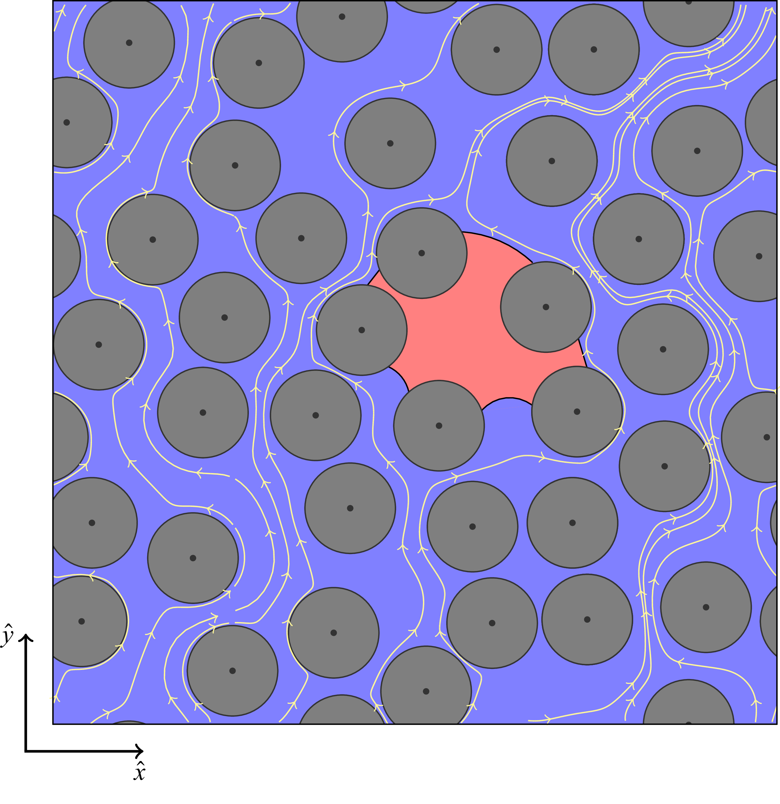
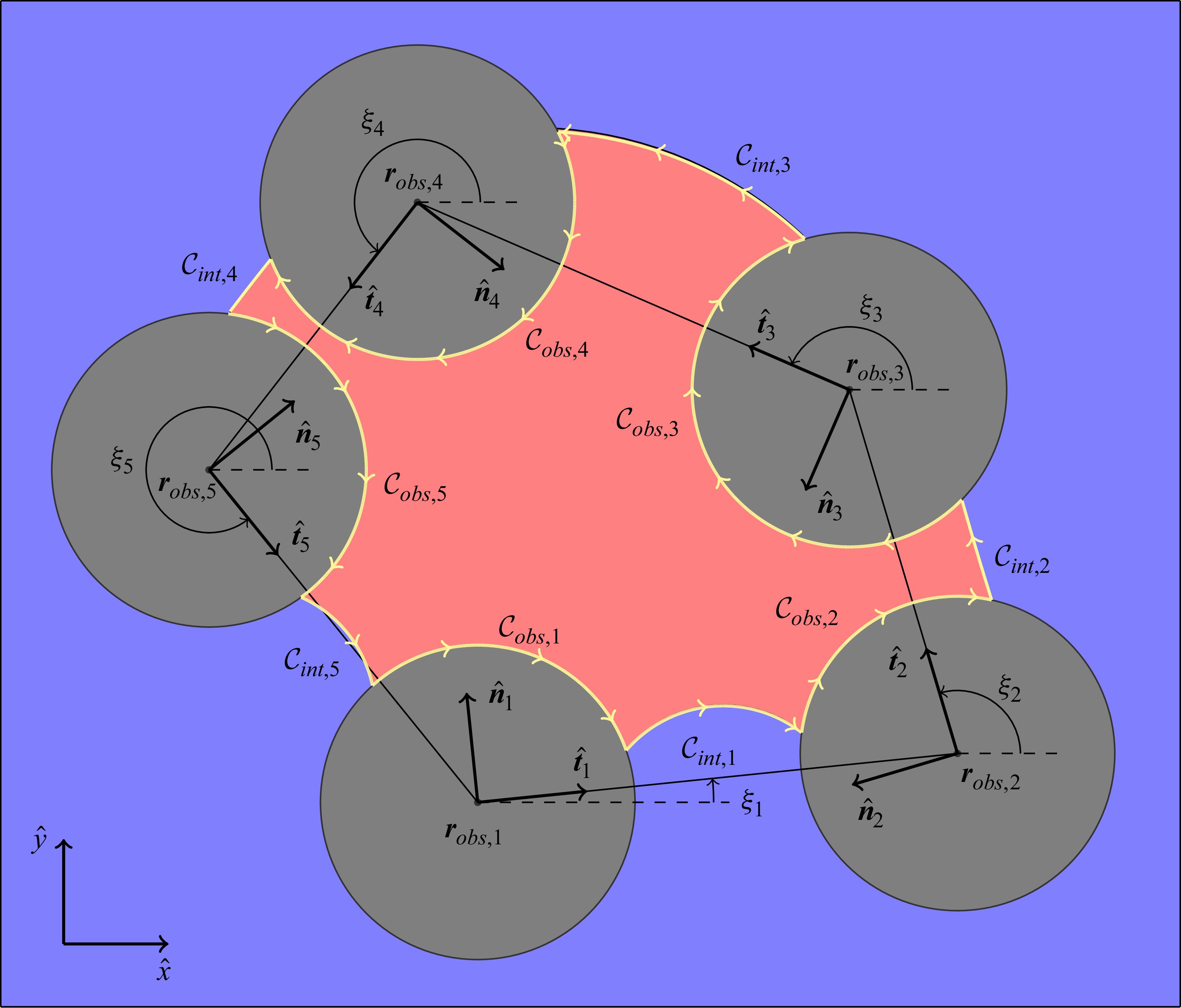
 n
n robs,n
 {t^n,n^n}
 t^n
t^n x
x ξn
ξn C
C Cint,n
 Cobs,n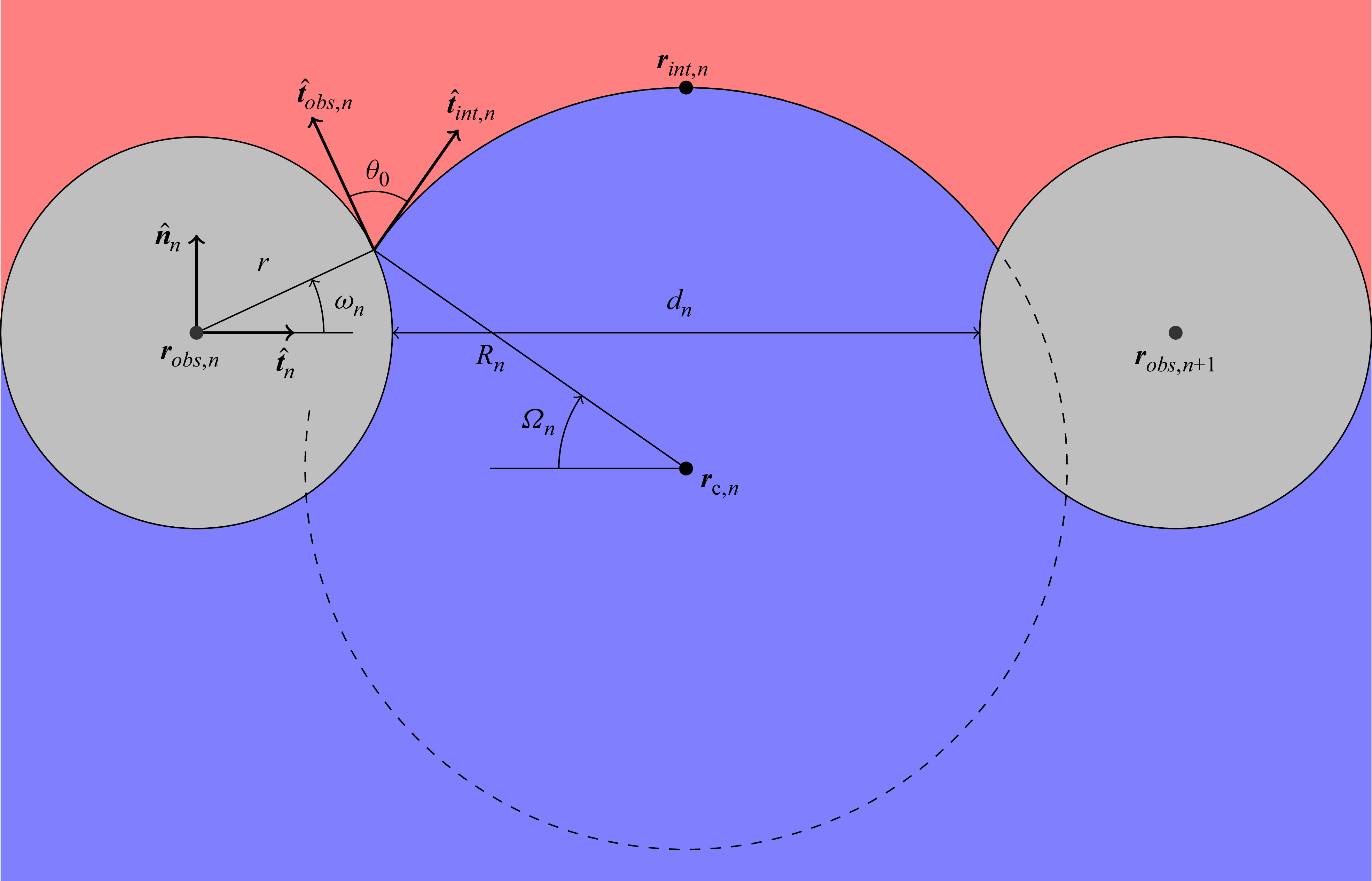
 n
n robs,n
 robs,n+1
 {t^n,n^n}
 Rn
Rn rc,n
rc,n rint,n
 t^obs,n
 t^int,n
 θ0
θ0 ωn
ωn t^n
t^n Ωn
Ωn −t^n
−t^n dn
dn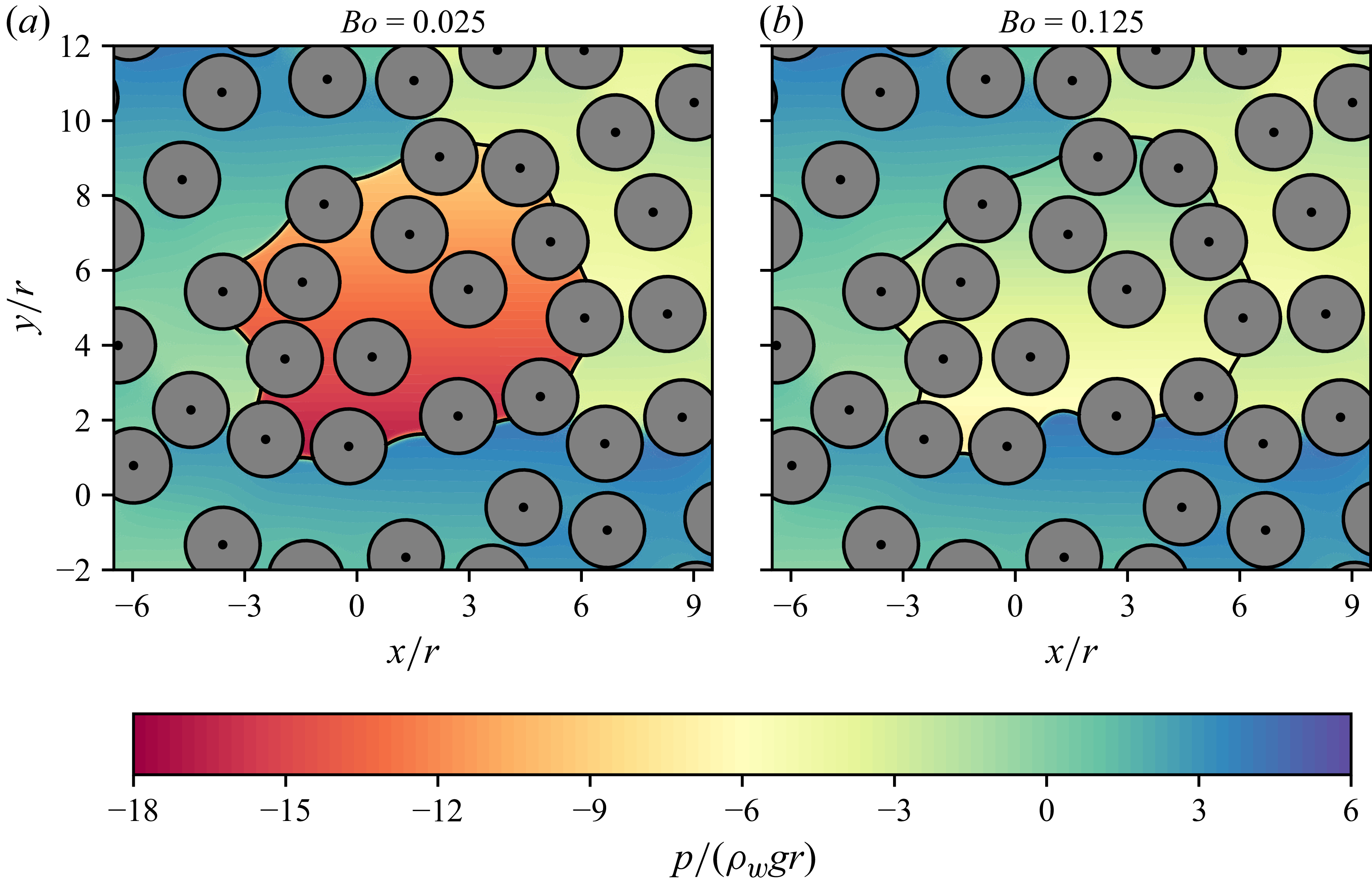
 Bo=0.025
 Bo=0.125
 Ca=0.00025
 Ca=0.00125
 Bo
Bo Bo
Bo rcircle/r=4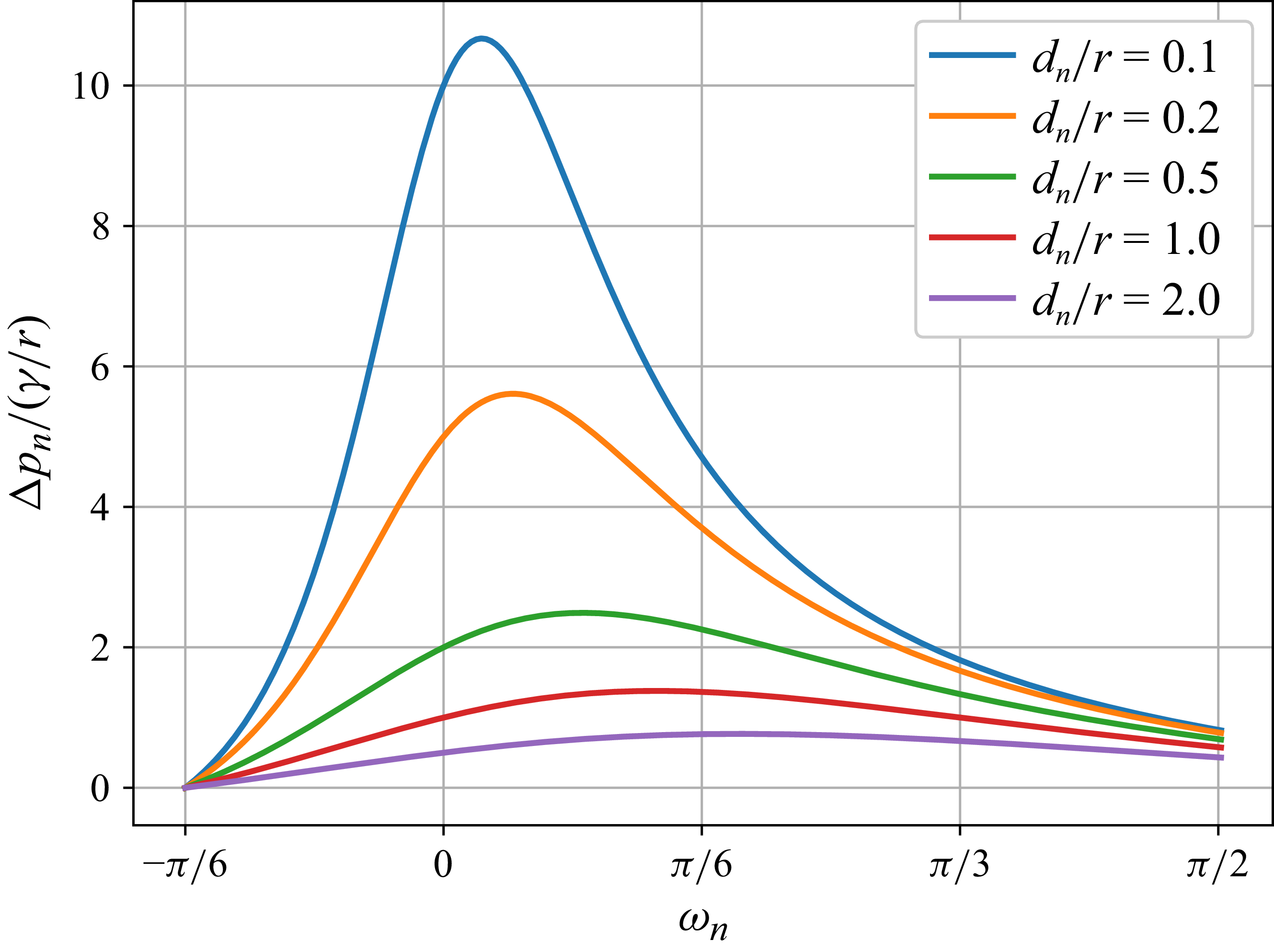
 n
n ωn
ωn θ=π/3
θ=π/3 dn/r
dn/r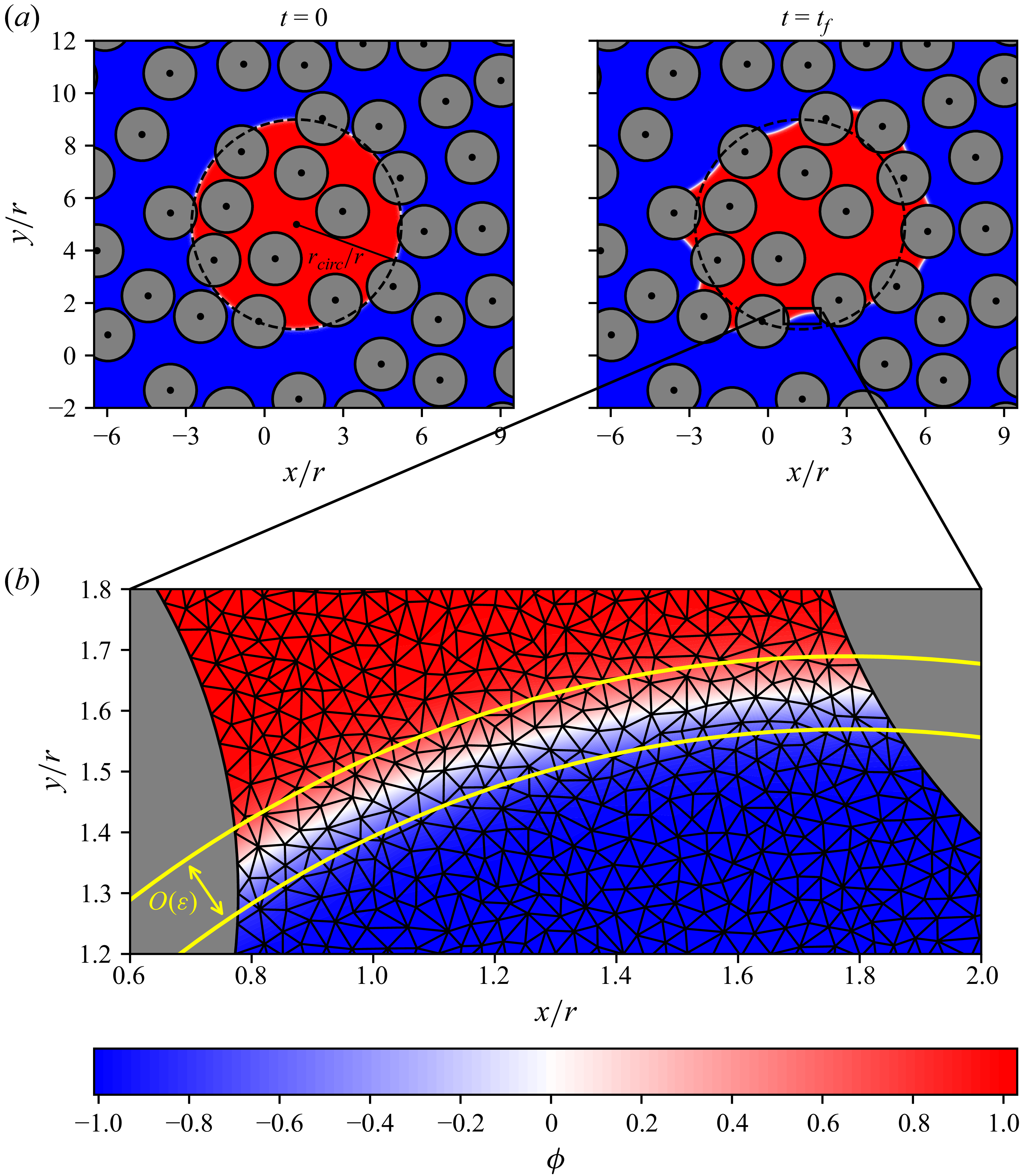
 rcirc/r=4
 Bo=0.025
 θ0
θ0 ϵ
ϵ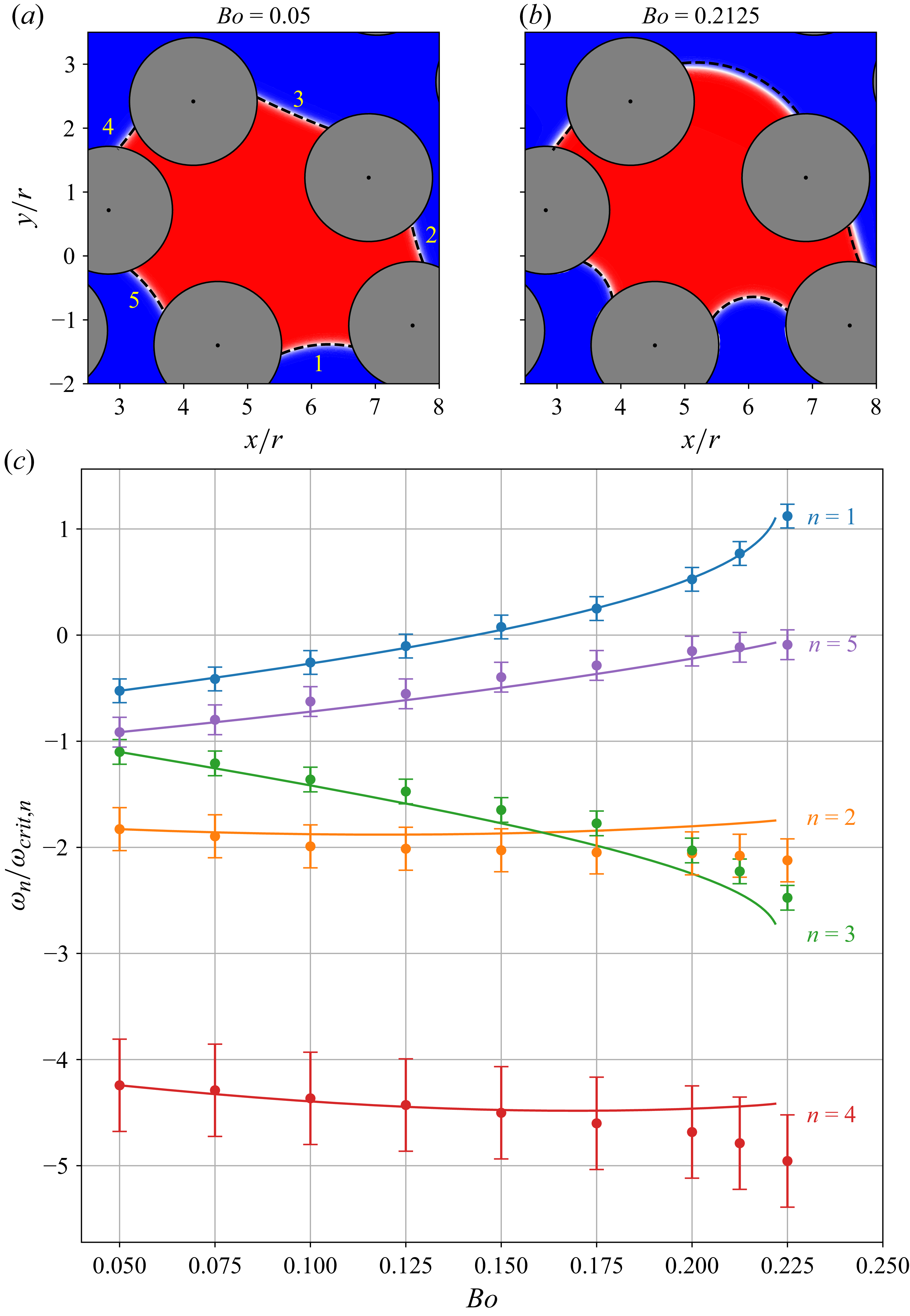
 rcirc/r=2
 Bo=0.05
 Bo=0.2125
 Bo=0.05
 ωn
ωn ωn
ωn ±ϵ
±ϵ n=1,2,…,5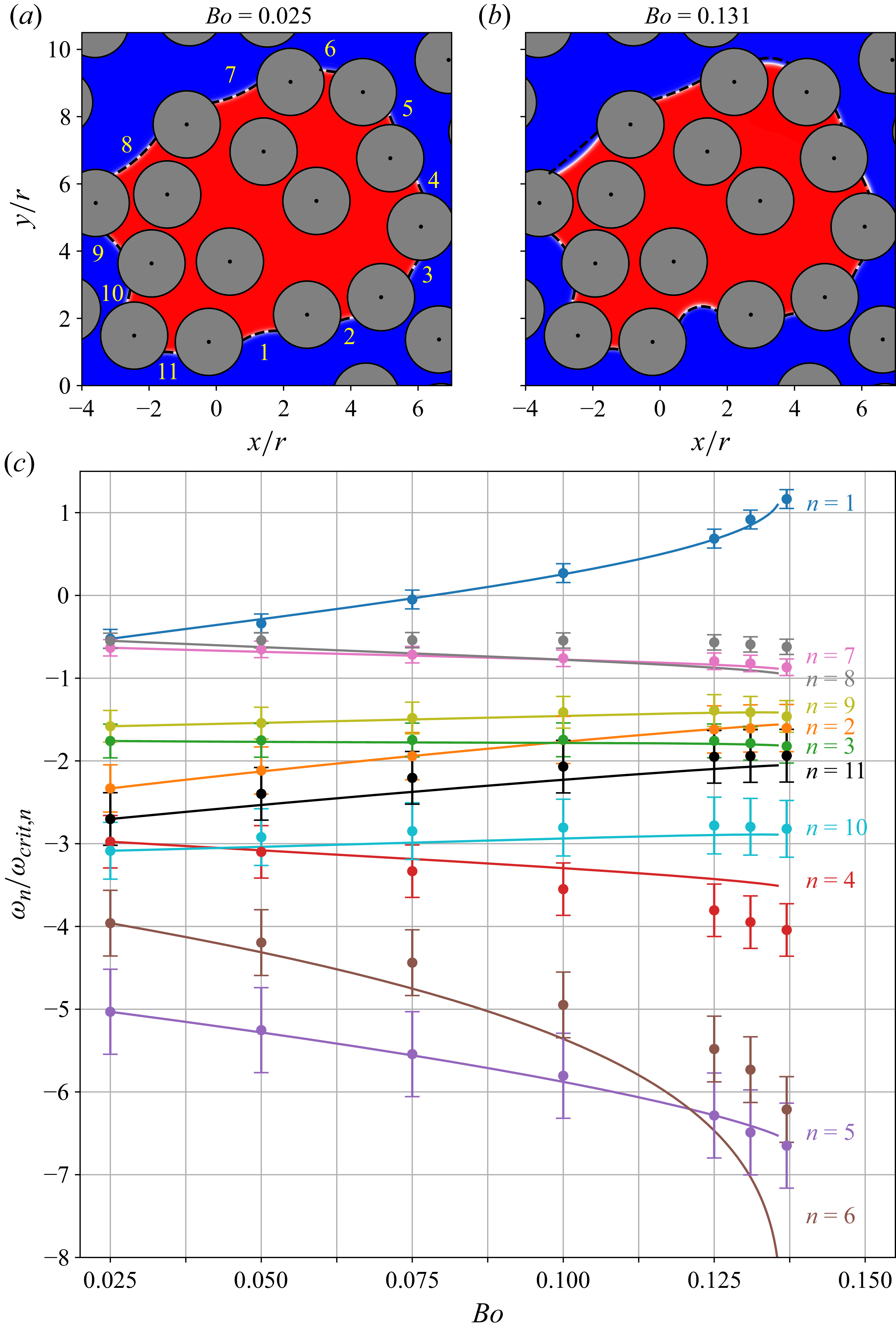
 rcirc/r=4
 Bo=0.025
 Bo=0.131
 Bo=0.025
 ωn
ωn ωn
ωn ±ϵ
±ϵ n=1,2,…,11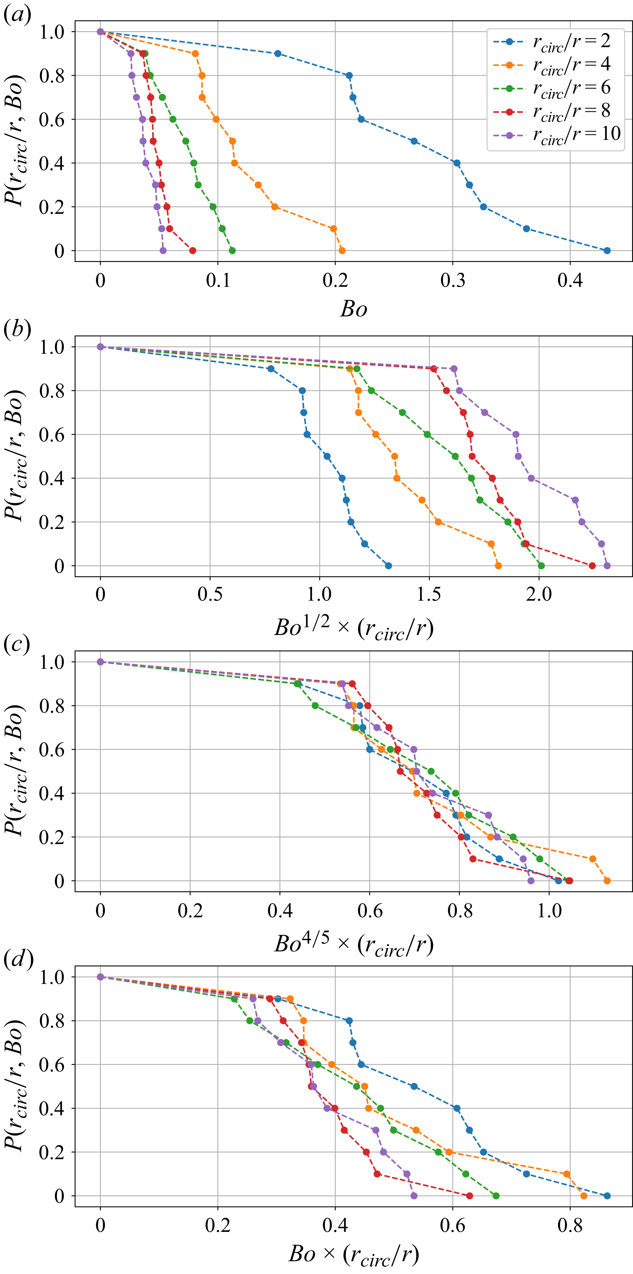
 rcirc/r
 Bo
Bo Bo1/2×(rcirc/r)
 Bo4/5×(rcirc/r)
 Bo×(rcirc/r)
 P(rcirc/r,Bo)
 Bo×(rcirc/r)
 Bo1/2×(rcirc/r)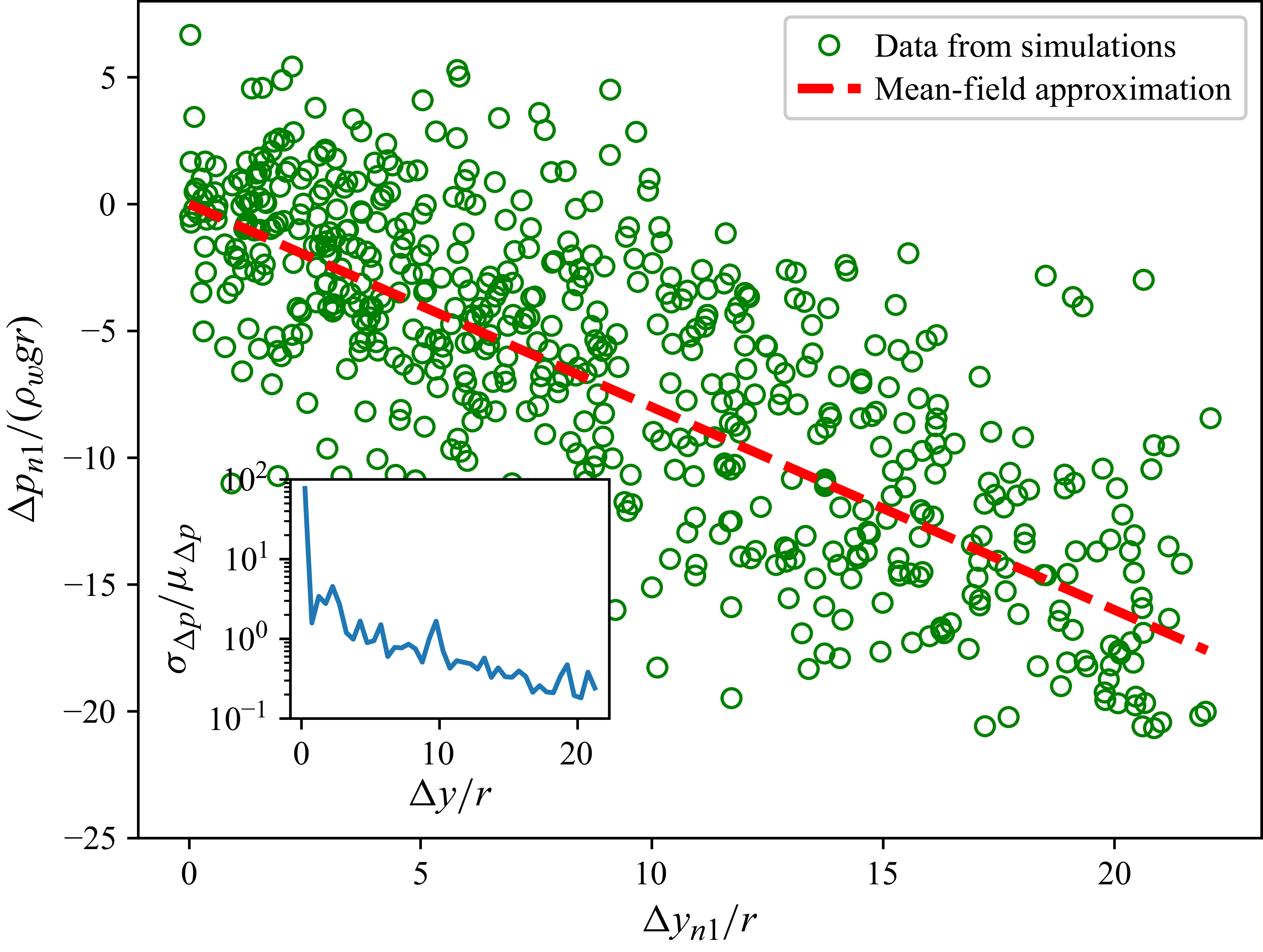
 Δpn1≡pout,n−pout,1
 y
y Δyn1≡yout,n−yout,1
 rout,n≡rint,n−δn^n
 δ=3ϵ
δ=3ϵ σΔp
σΔp μΔp
μΔp y
y m/2⩽Δy/r<(m+1)/2
 m=0,1,2,…
 σΔp≃3ρwgr
 Δy
Δy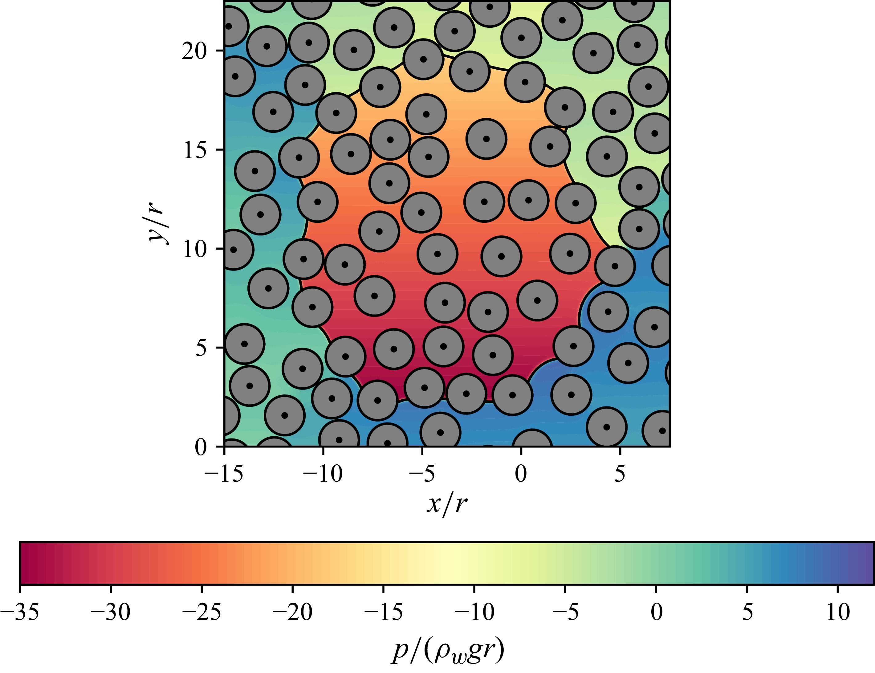
 rcirc/r=8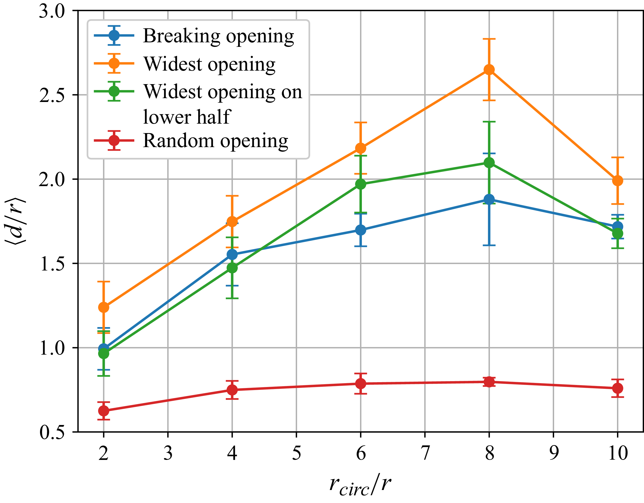
 rcirc/r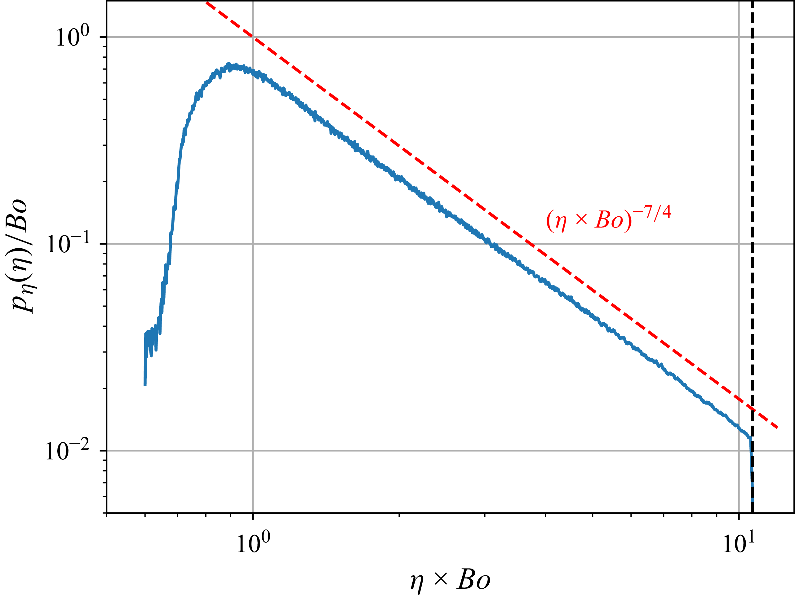
 η
η θ0=π/3
 d/r
d/r d
d dmin=r/10
 (η×Bo)−7/4
 pη
pη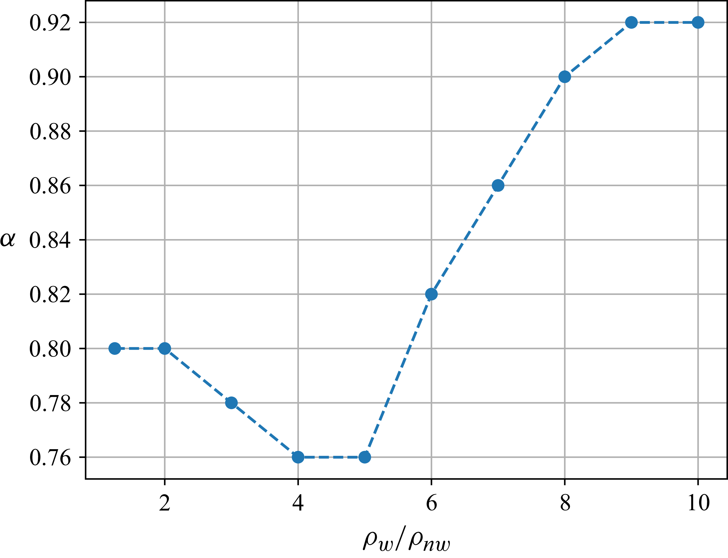
 α
α ρw/ρnw
 rcirc/r
 Boα×(rcirc/r)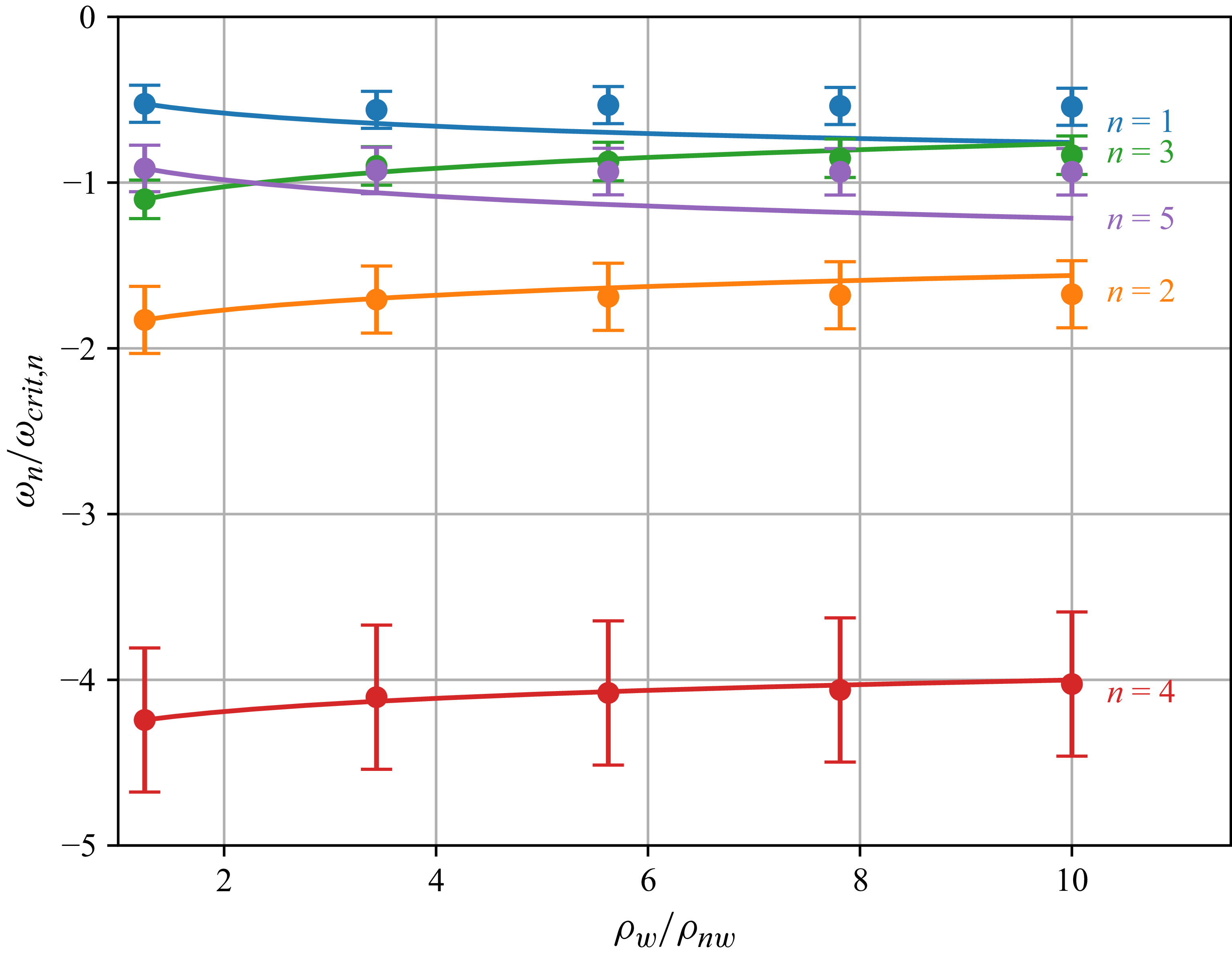
 ωn
ωn Bo=0.05
 ωn
ωn ±ϵ
±ϵ n=1,2,…,5
 Open access

