

1. Introduction
Surge-type glaciers undergo quasi-periodic cycles between slow (quiescent) and fast (surge) flow modes, and make up ~1% of the global glacier population (Jiskoot and others, Reference Jiskoot, Boyle and Murray1998; Sevestre and Benn, Reference Sevestre and Benn2015). Surge-like instabilities have also been invoked to explain oscillatory behaviour of ice sheets, including those thought to be responsible for Heinrich events (e.g. MacAyeal, Reference MacAyeal1993; Calov and others, Reference Calov, Ganopolski, Petoukhov, Claussen and Greve2002; Feldmann and Levermann, Reference Feldmann and Levermann2017). Although surge-type glaciers exhibit a range of thermal regimes, geometries and behaviours, it has been proposed that all can be understood in terms of enthalpy balance theory, which is based on coupled glacier mass and enthalpy (internal energy) budgets (Benn and others, Reference Benn, Fowler, Hewitt and Sevestre2019). The theory predicts that, for certain climatic conditions and glacier geometries, glaciers cannot achieve stable steady states with regards to their mass and enthalpy budgets, and consequently undergo oscillatory flow cycles, gaining mass and enthalpy progressively during quiescence and losing them dramatically during surge and surge termination.
Enthalpy balance theory is consistent with global-scale correlations between surging behaviour and climatic and geometric variables (Sevestre and others, Reference Sevestre, Benn, Hulton and Baelum2015; Benn and others, Reference Benn, Fowler, Hewitt and Sevestre2019). In this paper, we aim to test the theory at the scale of a single glacier, using detailed observations of a recent surge of Morsnevbreen, Svalbard. In addition, we investigate the ways that evolution of the surge was impacted by spatial phenomena not included in the current implementation of the theory.
2. Enthalpy balance theory
For an incompressible ice mass, enthalpy is defined as the internal energy of the ice, a function of ice temperature and liquid water content (Aschwanden and others, Reference Aschwanden, Bueler, Khroulev and Blatter2012). During glacier flow down a slope, gravitational potential energy is converted into enthalpy through frictional heating, mostly at or close to the bed. Enthalpy is also gained at the bed from geothermal heating. Enthalpy gains are manifest as warming of cold ice or melting of temperate ice. Conversely, enthalpy may be evacuated from the bed via heat conduction to the surface or meltwater discharge. Because both ice deformation rates and sliding speeds are sensitively dependent on ice temperature and water storage, any change in enthalpy at or near the bed will produce a dynamic response. Thus, for a glacier to maintain a stable steady state, enthalpy gains must match enthalpy losses, the rate of ice flow must match the balance flux, and the system must be stable to small perturbations. Any mismatch may lead to unsteady behaviour, including surges. Benn and others (Reference Benn, Fowler, Hewitt and Sevestre2019) presented a numerical model of these processes, following the lumped approach developed by Fowler (Reference Fowler1987) and Fowler and others (Reference Fowler, Murray and Ng2001). The key components of the system are expressed as a pair of differential equations describing mass and enthalpy conservation, respectively:


Equation (1) expresses the rate of change in mean ice thickness H over a reservoir zone of length l in terms of the surface mass balance (accumulation rate $\dot{a}$ minus net melt rate $\dot{m}$
 ) and export of ice by flow, Q i (it is assumed that no ice enters the reservoir zone by flow). Equation (2) describes the mean rate of change of enthalpy E at the glacier bed, where τ is the basal shear stress, u is the sliding velocity, $\dot{\varepsilon}$
 is the shear strain rate in the basal ice, τu is the frictional heating from sliding, $\tau \dot{\varepsilon} d$
 is the frictional heating from shear in a basal ice layer of unit thickness d, G is the geothermal heating, β is the proportion of surface meltwater reaching the bed, q i is the conductive heat flux, ρ is the water density, L is the latent heat of fusion and Q w is the water discharge from the bed. The first four terms on the right-hand side of Eqn (2) are enthalpy sources, and last two are enthalpy sinks.
These coupled equations express the key idea at the core of enthalpy balance theory: that mass and enthalpy fluxes are co-dependent and together govern glacier dynamic behaviours. Depending on input values of accumulation rate, air temperature, glacier length, bed slope and hydraulic conductivity, solutions to Eqns (1) and (2) exhibit either stable or unstable (oscillatory) behaviour (Benn and others, Reference Benn, Fowler, Hewitt and Sevestre2019). The model predicts stable steady states (non-surge-type glaciers) in both cold, dry environments and warm, humid environments, and unstable steady states (surge-type glaciers) in intermediate climates, in close agreement with the global distribution of surge-type and non-surge-type glaciers (Sevestre and Benn, Reference Sevestre and Benn2015). Variations in glacier geometry and basal hydraulic conductivity also influence surging behaviour, producing an overlap between surge-type and non-surge-type glaciers in the intermediate climates.
A crucial next step is to test predictions of enthalpy balance theory against data from individual glaciers. Because of the idealised ‘lumped’ nature of the model, we do not aim to replicate observations exactly, but to determine whether observed dynamic and thermodynamic changes over a surge cycle are consistent with model predictions. Figure 1 shows output of the model with input parameters broadly representative of glaciers in eastern Svalbard ($\dot{a} = 500\,{\rm mm}\,{\rm a}^{-1};\;\; T_{\rm a} = -7^\circ {\rm C}$ ). Output values of ice thickness H, basal enthalpy E and ice velocity u are normalised averages over an idealised glacier reservoir area of length 5 km and gradient 0.03.
Simulated surge cycles using the lumped enthalpy balance model of Benn and others (Reference Benn, Fowler, Hewitt and Sevestre2019), with (a–h) and without (i–p) input of surface water via crevasses. Panels e–h and m–p show detailed views of the surge phase (shaded regions in a–d and i–l). Variations in ice thickness H, basal enthalpy E and ice velocity u are normalised to reference values H 0, E 0 and u 0. The enthalpy variable E is scaled such that negative values represent the ‘cold content’ of ice below the melting point, and positive values represent water storage at a temperate glacier bed. Panels d, h, l and p show the enthalpy balance components: inputs of surface water, geothermal heating, frictional heating, conductive cooling and water discharge from the bed (solid lines are sources, dotted lines are sinks).
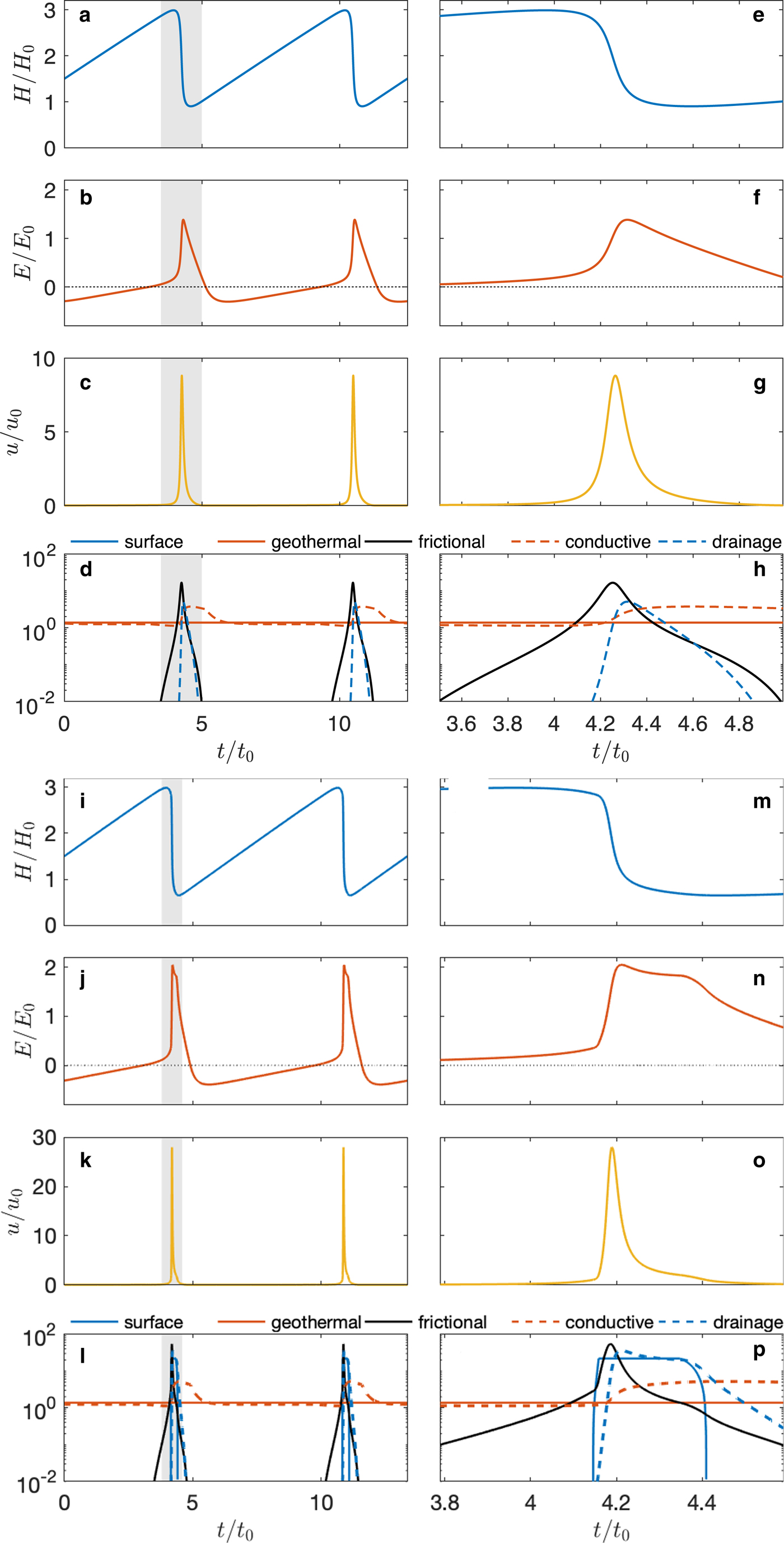
Output from two versions of the model is shown. In model 1, enthalpy is produced at the bed by geothermal and frictional heating, with no input of water from the glacier surface (Figs 1a–h). In model 2, an additional enthalpy source is provided by meltwater from the glacier surface at a rate proportional to ice velocity, to approximate the effect of increased crevassing on faster-flowing ice (Figs 1i–p). Both versions of the model show long quiescent periods interspersed with short-surge phases. During quiescence, ice velocities are very low, and ice thickness builds up almost linearly through snow accumulation. Enthalpy slowly increases during quiescence because gains from geothermal heating exceed losses from either conduction or water discharge. In model 1, frictional heating begins to contribute significantly to the basal enthalpy budget in late quiescence, and heating-velocity feedbacks cause an exponential increase in enthalpy at the bed. The surge phase is characterised by rapidly increasing velocities and drawdown of ice thickness. In model 2, velocity begins to increase as a result of geothermal and frictional heating as before, then surface meltwater begins to access the bed as a result of increasing crevassing. The additional water input increases the velocity, which accelerates frictional heating, thus supplementing the friction-velocity feedback with a more rapid crevassing-velocity feedback (Fig. 1p). Basal enthalpy and velocity increase more rapidly and attain higher values than those in model 1 (Figs 1n, o). In both cases, surge termination occurs when water is discharged from beneath the glacier faster than it is supplied.
Thus, enthalpy balance theory predicts that:
• during quiescence, enthalpy gains are primarily due to geothermal heating. Although small, these gains exceed losses via conduction;
• once sliding is initiated, frictional heating becomes a significant enthalpy source and positive feedbacks between frictional heating and ice velocity initiate the active phase of the surge; and
• crevasse formation and drainage of surface meltwater to the bed can reinforce these feedbacks, causing further flow acceleration.
We use high temporal- and spatial-resolution data from a recent surge of Morsnevbreen, Svalbard, to determine whether these predictions of the theory correspond to observed changes in the enthalpy balance of a polythermal glacier over the surge cycle. Published data (Nuth and others, Reference Nuth, Moholdt, Kohler, Hagen and Kääb2010) provide information on the second half of the quiescent phase (1936–1990), while our data cover the transition from late quiescence (1990–2010), through flow acceleration (2013–2016), to surge termination (2017–present). In addition, we examine the extent to which surge evolution is controlled by spatial effects not included in the lumped model.
3. Study area and methods
3.1 Study area
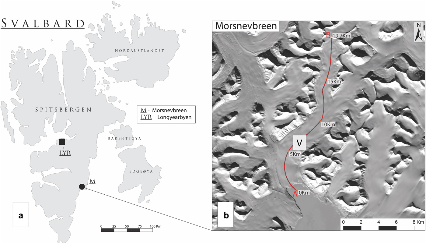
Morsnevbreen (77° 30′ N 17° 32′ E) is a major tributary of Strongbreen, a tidewater glacier that terminates in a 2.6 km wide calving front in Kvalvågen fjord in south-east Spitsbergen, Svalbard (Fig. 2). In 2010, prior to the recent surge advance, Morsnevbreen/Strongbreen was 19 km in length and had an area of 74 km2. The upper glacier consists of two main tributaries fed by ice from several cirques (hereafter, the upper tributaries); the tributaries converge at an altitude of 400 m a.s.l. to form the central trunk, which in turn flows into the lower glacier of Strongbreen at an altitude of 200 m a.s.l. The equilibrium line altitude (ELA) of the Strongbreen system is given as 280 m by Lefauconnier and Hagen (Reference Lefauconnier and Hagen1991), calculated assuming an accumulation area ratio of 0.7. A Landsat image from 20 August 2013 (near the end of the Svalbard ablation season) shows a snowline elevation of ~300 m, which we adopt as a nominal recent ELA for the glacier. Morsnevbreen/Strongbreen surged between 1870 and 1876 (Lefauconnier and Hagen, Reference Lefauconnier and Hagen1991), since which time the glacier underwent steady calving retreat until the front began to advance in October 2016 during the recent surge.
(a) Svalbard, showing location of Morsnevbreen and Longyearbyen weather station. (b) Morsnevbreen, with location of the centreline profile used for measurements and calculations. V indicates the location of the velocity time series shown in Figure 6.
3.2 Digital elevation model (DEM) differencing
Elevation changes on the glacier prior to and during the surge were determined by differencing pairs of DEMs. High-quality DEMs were available for late summer 1990 (Norwegian Polar Institute), December 2010 (ASTER), February 2014 (TanDEM-X) and November 2017 (ASTER). The DEMs were co-registered and adjusted to a common base elevation, using off-glacier areas (cf. Pritchard and others, Reference Pritchard, Murray, Strozzi, Barr and Luckman2003). DEM subtraction was performed between the 2017, 2014, 2010 and 1990 DEMs, allowing reconstruction of the sequence of elevation changes Morsnevbreen underwent during this 27-year period. In addition, changes in glacier elevation between 1936 and 1990 were derived from Figure 6 in Nuth and others (Reference Nuth, Moholdt, Kohler, Hagen and Kääb2010), which was based on the 1990 NPI DEM and a DEM constructed from oblique aerial photographs from 1936. The error associated with the differenced 1990 to 2010 DEM pair is low, with a std dev. of σ = 0.365 m for the off-glacier areas used for co-registration. The equivalent std dev. are higher for 2014–2010 (1.827 m) and 2017–2014 (1.990 m), possibly reflecting errors over steep terrain in the 2014 TanDEM-X DEM.
3.3 Bed DEM
The subglacial topography below Morsnevbreen was taken from a Svalbard-wide map product (SVIFT 1.0: https://doi.org/10.21334/npolar.2018.57fd0db4) created using a mass conservation approach informed by glacier geometry, elevation changes, surface mass balance and surface velocities (Fürst and others, Reference Fürst2018). For Svalbard, over 1 million point measurements on ice thickness were assimilated. For Morsnevbreen, the reconstruction was constrained by four airborne ice-penetrating radar profiles acquired in 1986 by Scott Polar Research Institute. These thickness values show a mean of 231 m and a maximum of 345 m in the central trunk. The reconstructed ice-thickness map has a somewhat smaller average of 127 m with an associated overall uncertainty of 9 m.
3.4 Ice surface velocities
Surface velocities for the period of February 2013 to November 2015 were derived from TerraSAR-X images in sequential pairs, acquired every 11 days. Feature tracking was applied in slant range using correlation windows of 200 × 200 pixels (~400 m × 400 m) spaced every 20 pixels (~40 m) and the resulting images were ortho-rectified to a pixel size of 40 m using the 2014 DEM (Luckman and others, Reference Luckman2015). Uncertainties in surface velocity were due to co-registration error (±0.2 pixels) and through smoothing of the velocity field over the feature-tracking window size. These uncertainties were estimated to be better than 0.1 m d−1, and the TerraSAR-X images were therefore ideal for detecting the small velocity changes occurring during the initial stages of the surge. During the summer months, however, the quality of velocity retrievals was often reduced by poor radar reflectance under melt conditions and the loss of coherent speckle for feature tracking.
Surface velocities for the period of March 2016 to January 2019 were derived from Sentinel-1 Interferometric Wide Swath mode SAR images in sequential pairs, acquired every 12 days until September 2016, then subsequently every 6 days. Feature tracking was applied in slant range using correlation windows of 416 × 128 pixels (~1 km2) spaced every 50 × 10 pixels (~100 m) and the resulting images were ortho-rectified to a pixel size of 100 m using the 2014 DEM. Uncertainties in Sentinel-1 velocities are estimated to be better than 0.4 m d−1. To summarise the spatial and temporal evolution of surface velocities during the surge, data were extracted for profiles along the glacier centre line (Fig. 2). Data points were taken every 100 m along the line for each pair, and the results were plotted into Hovmoller time-distance diagrams.
3.5 Crevasses and surge front evolution
Landsat-7 and 8 scenes were used to create maps of crevasse distribution on the glacier surface. Band-8 panchromatic images were selected due to their relatively high resolution of 15 m. Crevasses were identified and hand-digitised in ArcMap. For several reasons, the crevasse maps are incomplete. Crevasses can be obscured by snow cover, clouds or shadows, and the resolution of the images meant that only large, wide crevasses could be detected. Despite this, the resulting maps produced an effective means of showing how the surface of Morsnevbreen changed as the surge developed, and indicate areas where surface to bed meltwater drainage could occur.
Propagation of the surge front was determined from the velocity maps and Landsat-7 and 8 images. The surge-front was assumed to be located at the downglacier boundary of ice with detectable motion, and arcuate shadows visible on the optical images.
3.6 Climate data
Daily surface air temperature and precipitation data were downloaded from the Norwegian Meteorological Institute via the ‘statistics’ pages of their website (https://www.yr.no/). The most proximal weather station at Longyearbyen Airport (Fig. 2) was chosen, which lies 83 km north-west of Morsnevbreen at 28 m a.s.l. and 400 m from the ocean. The time-period for the observations presented is October 2015 to February 2019.
3.7 Enthalpy balance calculations
For two reasons, we calculate the enthalpy balance at the glacier bed using a reduced form of Eqn (2). First, enthalpy production due to shear in basal ice, $\tau \dot{\varepsilon} d$ , was found to be negligibly small in all cases. Even where driving stresses were highest, this term only reached ~60 µW m−2, three orders of magnitude less than geothermal heating. Second, we have no quantitative data on the proportion of surface meltwater reaching the bed or subglacial water discharge. As will be shown, the omission of water balance is appropriate for the early stages of the surge, and for the later stages we consider the effect of water balance qualitatively. Thus:

Shear strain rate in the basal ice was calculated from Glen's flow law:

The rate factor A was set to be 2.4 × 10⁻²⁴ Pa−3 s−1, appropriate for 0°C, and n = 3 (Cuffey and Paterson, Reference Cuffey and Paterson2010). Driving stresses were calculated from:

where g is the gravity and α is the surface slope (Hooke, Reference Hooke2005). Values of H and α were obtained from the bed DEM and the surface DEMs for 1990, 2010, 2014 and 2017. Surface slope and driving stress were averaged over 2000 m, or ~5–10 ice thicknesses, to smooth out the effect of longitudinal stress gradients (Bindschadler and others, Reference Bindschadler, Harrison, Raymond and Gantet1976).
Sliding rate u was calculated using two methods. First, for periods when velocity data were available, u was calculated from observed surface velocities minus the calculated deformational component of surface velocity u d, obtained by integrating Eqn (4) from the bed to the surface:

Velocities were calculated by this method for May 2013, May 2014 and September 2014 using the February 2014 DEM for ice thickness and gradient data, and for November 2017 using the contemporary DEM.
Second, for the important early periods 1990–2010 and 2010–2014, we calculated average rates of potential energy expenditure from elevation differences between DEMs, modifying the continuity equation (1) to obtain:

where Q i(x) is the annual ice discharge at successive distances x down the glacier centre line (m3 a−1 per unit width), Δh is the annual elevation change determined from successive DEMs and b is the annual surface mass balance estimated from the 1936–1990 elevation differences (Nuth and others, Reference Nuth, Moholdt, Kohler, Hagen and Kääb2010). The values of b are consistent with mass balance data from elsewhere in Svalbard (Hagen and others, Reference Hagen, Kohler, Melvold and Winther2003). Sliding velocity was calculated by subtracting the deformational component of ice discharge from Q i, and dividing by H:

where H and α were obtained from the earlier DEM from each pair.
Conductive heat flux q i was calculated using a linear, steady state equation:

where k is the thermal conductivity of ice (2.25 W m−1 K−1), T b is the basal temperature, T s is the ice surface temperature and H is the ice thickness (Hooke, Reference Hooke2005). We take this approach rather than using a differentiated, time-evolving heat flux equation because of lack of data on the thermal history and water content of the ice. Equation (9) was primarily used to determine areas of the terminal zone where basal freezing could occur. For this purpose, it was initially assumed that the basal temperature was 0°C and the near-surface ice temperature equal to the mean annual air temperature at sea level in Svalbard, i.e. −5°C (Nordli and others, Reference Nordli, Przybylak, Ogilvie and Isaksen2014). The rate of geothermal heating G was taken to be 0.065 W m−2 (Etzelmüller and others, Reference Etzelmüller2011).
Errors in calculating frictional heating reflect uncertainties in ice velocity and thickness. Taking errors in velocity and ice thickness as independent and additive, we find errors in frictional heating of ±0.01 W m−2 for calculations using TerraSAR-X data and ±0.04 W m−2 for calculations derived from Sentinel-1 data. For frictional heating derived from TerraSAR-X velocities, errors are relatively large (~15%) for the upper tributaries in the early stages of the surge, where the ice is relatively thin and observed velocities are low, but are relatively small for the central trunk (1–6%), due to thicker ice and higher velocities. For frictional heating values derived from Sentinel-1 data, the relative error is small (1–3% in the central trunk; ~8% in the upper tributary) because of the higher ice velocities during the later stages of the surge. Errors in calculated conductive heat losses are ~0.003 W m−2, or ~6% in the lower glacier where ice is relatively thin.
4. Observations of surge evolution
4.1 Geometric changes
Between 1936 and 1990, the glacier underwent thickening above 288 m a.s.l., and thinning below that altitude (Nuth and others, Reference Nuth, Moholdt, Kohler, Hagen and Kääb2010; Fig. 3). Thinning rates on the lower glacier varied linearly with altitude, whereas thickening on the upper glacier increased to 0.75 m a−1 at ~450 m a.s.l. and remained roughly constant above that altitude. Between 1990 and 2010, the lower ablation zone of Morsnevbreen continued thinning with an ablation gradient closely similar to that of 1936–1990 (Figs 3, 4a). Above 185 m a.s.l., the elevation change curve diverged from the ablation gradient and values became positive above 245 m a.s.l., consistent with dynamic thickening. In contrast, ice in the upper tributaries underwent thinning of up to 1 m a−1.
Vertical profiles of elevation change along the glacier centre line, 1936–1990; 1990–2010; 2010–2014 and 2014–2017.

Annual rates of elevation change for 1990 to 2010, 2010 to 2014 and 2014 to 2017.

Between 2010 and 2014, the lower glacier continued to thin, the central trunk thickened substantially at ~6 m a−1, and much of the ice in the upper tributaries thinned (Figs 3, 4b). The downglacier limit of dynamic thickening ice moved 3.9 km downglacier between 2010 and 2014, coincident with the advance of a pronounced bulge (surge front) on the glacier surface. The zone of surface lowering in the upper tributaries also expanded downglacier. Dramatic changes in surface elevation occurred between 2014 and 2017; substantial thinning occurred above 270 m a.s.l., with maximum values >10 m a−1, while thickening at similar rates occurred over the lower glacier (Figs 3, 4c).
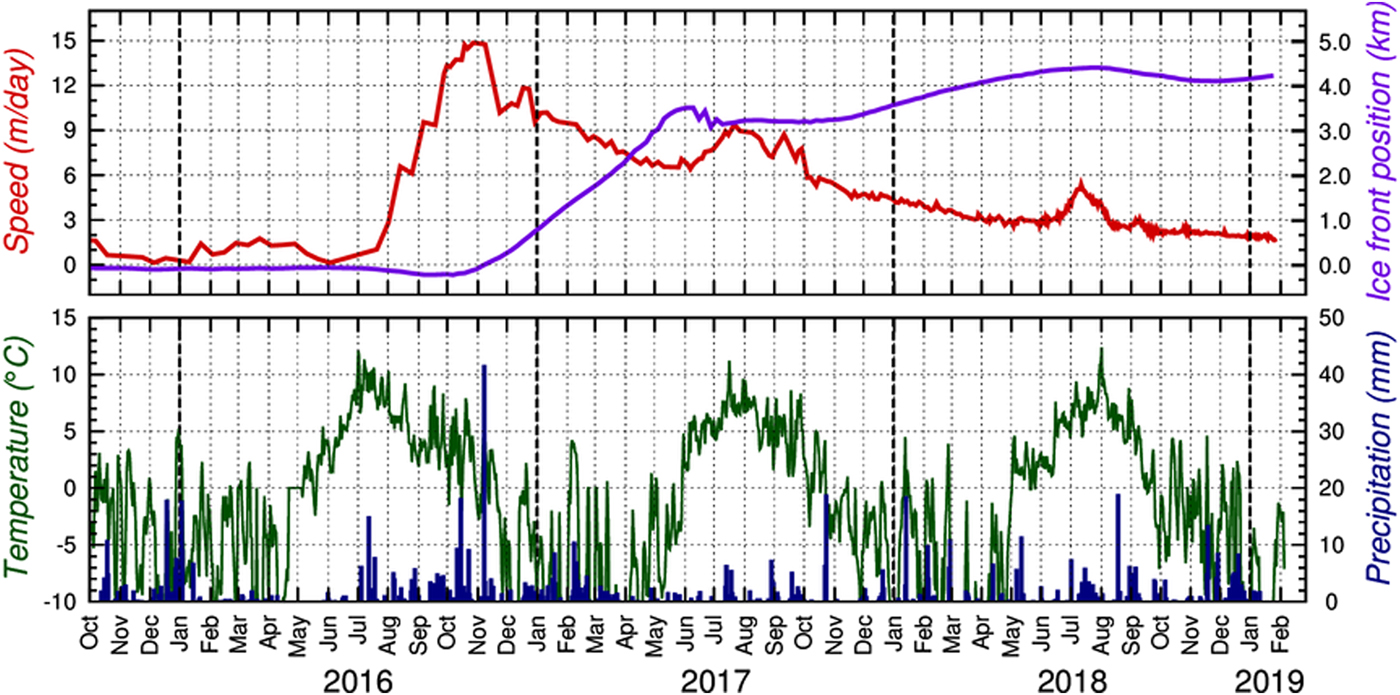
The surge front propagated ~4 km downglacier between March 2013 and October 2016 when it reached the terminus (Fig. 5). The rate of propagation was not constant, and three distinct phases can be identified: (1) from 19 March 2013 to 18 August 2014 the propagation rate averaged 7.6 m d−1; (2) between 18 August 2014 and 8 July 2016 this slowed to only 1.4 m d−1 and (3) after July 2016, the rate of surge-bulge propagation accelerated, reaching >40 m d−1 by September. As the surge front neared the terminus, the calving rate increased and the glacier entered a brief period of frontal retreat (Fig. 6). From October 2016 until mid-2017, the ice front advanced ~3.7 km until accelerated calving again brought about a period of ice front retreat and stillstand until October 2017. From then until mid-2018 the front underwent further advance of ~1.5 km, followed by another seasonal retreat-advance cycle.
Location of major crevasses and the surge front on selected dates. Lower right panel shows the advance of the surge front during 2013–2016. The y-axis shows distance down the flowline with an arbitrary origin.

4.2 Crevasse distribution
During 2013, large crevasses only occurred within a few hundred metres of the glacier terminus, where they trended parallel to the ice front (Fig. 5). This pattern is typical of Svalbard tidewater glaciers, and reflects longitudinal extension of the ice in response to the force imbalance at the terminal ice cliff (cf. Flink and others, Reference Flink2015). No crevasses are visible farther up-glacier on Landsat imagery until July 2014, when crevasses appeared along the margins of the central trunk, aligned obliquely up-glacier towards the centre line, and in the upper tributaries where they were oriented transverse to ice flow (Fig. 5b). The distribution of crevasses was similar in 2015, with continuing development of oblique and transverse fractures at the glacier margins and upper tributaries, respectively. In September 2015, shallow longitudinal crevasses were visible in the area of the surge bulge during an overflight of the glacier, but these were too narrow to be resolved on the Landsat images.
A major increase in the extent of crevasses occurred by August 2016 (Fig. 5d), when marginal and transverse crevassing developed over most of the glacier above 250 m a.s.l. Below this elevation, velocity data (see below) indicate the ice was in compression. After the terminus advance began in October 2016, large transverse crevasses developed over much of the glacier. The central and lower trunk became pervasively crevassed, with fractures so clustered together that at the resolution of the Landsat-8 optical imagery individual fractures can no longer be identified.
4.3 Velocity changes
The earliest available TerraSAR-X data (February 2013) indicate velocities up to ~0.25 m d−1 in the central trunk of Morsnevbreen (Fig. 7). Due to low image coherence, no data are available for the summer months, but by November velocities in the trunk region had increased to ~0.5 m d−1, and remained at that level throughout the winter. By autumn 2014, velocities had further increased to ~0.8 m d−1, and gradually increased further during the following winter (Fig. 8). The zone of elevated velocities had a well-defined lower boundary, coincident with the downglacier limit of thickening ice shown on the 2010–2014 elevation change map and the position of the surge bulge (Figs 4, 5, 7).
Maps of time-averaged TerraSAR-X velocity data, showing the early evolution of the surge.

Time-distance Hovmoller diagrams for (a) TerraSAR-X and (b) Sentinel velocity data along the glacier centre line. The vertical line in (b) indicates the position of the velocity time series shown in Figure 6.

An increase in velocity occurred in the warm summer months of 2015, reaching ~1.5 m d−1. A major change in the dynamics occurred in June 2016, when a sustained and dramatic acceleration occurred, synchronously with the increased rate of downglacier surge front propagation (Figs 5, 6). Maximum measured velocities reached ~6 m d−1 in mid-August and ~15 m d−1 in late October. The acceleration coincided with sustained positive air temperatures and frequent heavy rain events, which persisted until late October 2016. In that month, the surge front reached the glacier terminus, and the glacier advanced into the fjord. As the advance began, velocities began to fall, sharply at first and then more slowly. With the onset of positive air temperatures in June 2017, velocities increased once more, with the zone of fast flow extending >12 km from the glacier front. Following a slowdown in late August, a second velocity spike occurred in September, coincident with warm temperatures and rain. During winter 2017–2018, velocities steadily declined and had fallen to ~ 3 m d−1 by June 2018. Warm weather and rain in July brought another short-lived spike in velocities (to ~5 m d−1), after which they resumed the former declining trend (Fig. 6).
4.4 Synthesis
The evolution of Morsnevbreen before and during the surge can be summarised as follows:
Between 1936 and 1990 (about 60–100 years after the 19th century surge) the upper glacier thickened while the lower glacier thinned (Nuth and others, Reference Nuth, Moholdt, Kohler, Hagen and Kääb2010; Fig. 3). The pattern of elevation change closely follows published mass balance curves for Svalbard (Hagen and others, Reference Hagen, Kohler, Melvold and Winther2003), and shows no sign of modification by ice flow. This is typical quiescent-stage behaviour, with net accumulation in a reservoir zone above the ELA and net ablation on the lower glacier.
Between 1990 and 2010, the lower glacier continued to thin, while the central trunk thickened and drawdown of ice occurred in the upper tributaries. This period represents the onset of detectable mass transfer from the upper reservoir zone.
From 2010 to 2014 the rate of mass flux increased, with increasing velocities in the central trunk, downglacier displacement of the zone of thickening, and an expansion of the area of drawdown on the upper glacier. The surge front propagated downglacier at ~8 m d−1 during this period. These geometric and velocity changes were accompanied by the appearance of surface crevasses in 2014, consistent with lateral shearing and longitudinal extension on the central and upper glacier, respectively.
Surface velocities increased again during the warm months of 2015, then the peak phase of the surge began with the onset of summer melt in 2016. A rise in velocities up to 15 m d−1 coincided with a major acceleration of the surge-front propagation rate, which switched from ~1 m d−1 to tens of metres per day. The 2016 acceleration coincided with the widespread occurrence of crevasses above ~250 m a.s.l., which allowed surface water to access the glacier bed. Velocities fell at the terminus immediately after arrival of the surge front. Storage and release of basal water thus appear to be the key controls on velocities in the months before and after the surge peak in October 2016.
After the surge front reached the glacier terminus in early October 2016, Morsnevbreen began to advance, increasing the glacier length by 3.5 km by mid-2017. The downglacier-propagating wave of deceleration during the first half of 2017 is consistent with drainage of stored of water from the glacier bed, while the up-glacier propagating speed-up in June and July, the August slowdown and the September speed-up reflect changing balance between surface water input and basal drainage.
Advance of the glacier terminus was halted or reversed by calving in summer and autumn 2017, but resumed in November with a total advance of 4.5 km by July 2018. Velocities continued to decrease during 2018, interrupted by a speed up in the summer months suggesting that the balance between surface water input and basal drainage continued to influence glacier dynamics.
5. Enthalpy balance
To quantify key processes involved in the evolution of the surge, we now calculate components of the enthalpy balance at the glacier bed for selected times. A key first step is the calculation of driving stresses, which are required to obtain the frictional heating components (Eqn (3)). We then consider the thermal structure of the glacier, and ice discharge and sliding rates and associated enthalpy production. We conclude by presenting evidence for water discharge from the glacier and consider its implications for the basal drainage system.
5.1 Driving stresses
Driving stresses were calculated from the bed and ice-surface elevation data for late summer 1990, December 2010, February 2014 and November 2017 (Fig. 9). In 1990, the highest stresses (>60 kPa) occurred in the vicinity of a pronounced overdeepening in the glacier bed, where ice thickness reached >300 m. On the lower tongue, which was grounded a few tens of metres below sea level, driving stresses were lower (20–40 kPa), with intermediate values (40–50 kPa) in the upper tributaries. In 2014, driving stresses increased to >70 kPa at the overdeepening, reflecting thickening ice in this area. At the same time, driving stresses decreased in the upper glacier as a result of ice thinning. By 2017, driving stresses had fallen over the central and upper parts of the glacier as a consequence of glacier thinning, with typical values of 40–50 kPa on the central trunk and 20 kPa on the upper glacier. In contrast, stresses on the lower tongue increased sharply, reflecting the increase in ice thickness in this area.
(a) Bed and ice surface profiles along the glacier centre line and (b) calculated driving stresses.

5.2 Thermal structure of the glacier
No observations of the thermal structure of Morsnevbreen and Strongbreen are available. Abundant data on other similarly sized glaciers in Spitsbergen, however, allow its overall form to be inferred with confidence. Radio-echo sounding surveys show that larger valley glaciers in Spitsbergen have a two-layered thermal structure, with temperate ice at depth overlain by a cold surface layer up to 200 m thick (Bamber, Reference Bamber1987, Reference Bamber1989; Björnsson and others, Reference Björnsson1996; Sevestre and others, Reference Sevestre, Benn, Hulton and Baelum2015). The cold layer may be thin or absent in the accumulation area where temperate firn is formed each season by refreezing of meltwater, and conductive heat loss is small due to the low thermal conductivity of snow. In ablation zones, the cold layer can extend to the bed where ice is thin, including glacier margins and the lower tongues of land-based glaciers. Either cold or warm-based ice may occur at the termini of tidewater glaciers, depending on ice thickness (Sevestre and others, Reference Sevestre, Benn, Hulton and Baelum2015, Reference Sevestre2018). These considerations indicate that immediately prior to the recent surge, Morsnevbreen was warm-based below the central trunk, where ice was well over 200 m thick, and below much of the upper tributaries where the cold surface layer was likely thin. This conclusion is supported by evidence for ubiquitous sliding in the upper glacier during the study period (see section ‘Ice discharge and sliding during the surge’). Cold-based ice was possibly extensive in the upper tributaries in early quiescence, prior to the 20th century thickening.
Parts of the lower tongue of Morsnevbreen/Strongbreen may have been cold-based prior to the advance of the surge front in 2014. Between 1990 and 2014, driving stresses in this area were 20–35 kPa and calculated basal shear strain rates are very small. Enthalpy production rates at the bed from shear heating of the basal ice were the order of 1 µW m−2, ~4 orders of magnitude lower than geothermal heating. To a close approximation, therefore, enthalpy balance on the lower tongue can be characterised in terms of geothermal heating and conductive heat losses. From Eqn (9) we find that conductive heat losses exactly equal geothermal heating when H is equal to ~175 m. Thus, we conclude that the lower tongue of Morsnevbreen had the potential to freeze to the bed if H < 175 m.
In 1990, the lower tongue was >175 m in thickness except for narrow zones along the lateral margins (Fig. 10). By 2010, thinning of the ice had created a zone <175 m extending all the way across the glacier, and this had expanded by 2014. It is striking that the August 2014 surge front position, where surge-front propagation rate slowed from 7.6 to 1.4 m d−1, coincides with the location where ice thickness had declined to <175 m across the whole glacier. The abrupt slowing of surge-front propagation rate provides indirect corroborative evidence that a ‘barrier’ of cold-based ice existed on the lower tongue in 2014. Available DEMs between 1990 and 2010 are not of sufficient quality to determine when ice thinner than 175 m first extended all the way across the lower glacier. An estimate can be made, however, by extrapolating backwards from the 2010 ice thickness values using the measured rates of surface lowering. This indicates that a band of ice thinner than 175 m first extended across the lower glacier in 2003. However, basal freezing likely lagged after this date because time is required to conduct heat away from the bed. This cannot be calculated with any certainty due to the unknown water content at the glacier bed, but it can be concluded that a zone of cold-based ice likely extended across the lower tongue by the end of the period 1990–2010.
Thinning of the glacier from 1990 to 2014, showing the 175 m thickness contour which delimits the area of potential bed freezing. The 2003 map was derived by extrapolation back from the 2010 image, using measured changes in ice thickness.

5.3 Ice discharge and sliding during the surge
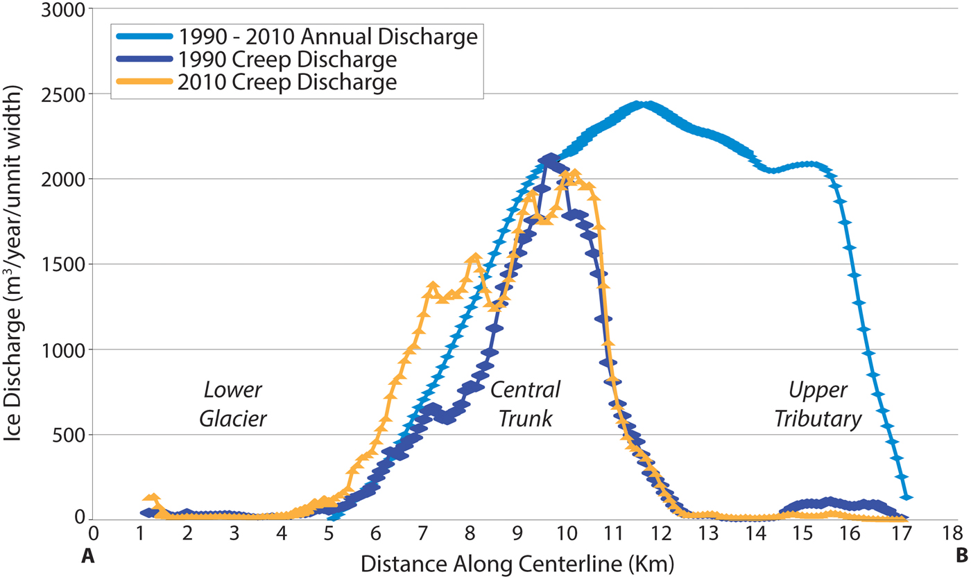
Calculations from continuity (Eqn (7)) show that between 1990 and 2010, average ice discharge increased from the top of the glacier to a maximum at 335 m a.s.l. (km 11.5 in Fig. 11), then decreased to zero at 185 m a.s.l. (km 5). Ice deformation can account for almost all of this discharge in the central trunk, but there is a large difference between total discharge and ice-creep discharge on the upper glacier, indicating sliding at rates of up to 15 m a−1 (Fig. 12). Ice discharge increased between 2010 and 2014, with average sliding speeds reaching ~70 m a−1 on the upper glacier. Significant sliding was also initiated on the lower trunk, with mean speeds up to 50 m a−1 (Fig. 12).
Calculated ice discharge 1990–2010, showing total flux and ice creep components.
Sliding velocities and enthalpy production rates 1990–2014.

The period 2010–2014 overlaps with the start of the TerraSAR-X velocity series, allowing comparison between the sliding speeds calculated from continuity and those derived from velocity observations and the February 2014 DEM (Fig. 12). On the upper glacier, data from May 2013 display a similar sliding mode to the 2010–2014 average, but sliding was more rapid in the central trunk. This is consistent with a rapid increase in sliding in the central trunk over the 2010–2014 period. By May 2014 (3 months after the end of the 2010–2014 period), sliding speeds in the central trunk had increased to ~0.4 m d−1 (~150 m a−1), ~50% higher than in the upper glacier. In September 2014, peak sliding speeds were in excess of 0.7 m d−1 (~250 m a−1) in the central trunk. The data thus show that sliding was initiated in the upper glacier between 1990 and 2010, and that this extended into the central trunk during 2010–2014 (Fig. 12). By 2013, the sliding speeds in the central trunk had overtaken those in the upper glacier, and rapidly climbed thereafter.
The date of the next DEM (November 2017) is after the surge peak and observed surface velocities had fallen to ~50% of the maximum values recorded for late 2016. Sliding accounts for almost all of the observed surface velocities of 3–5 m d−1 (1–1.8 km a−1).
5.4 Enthalpy production during the surge
Frictional heating associated with sliding increased dramatically over the course of the surge (Fig. 12). In the upper glacier, frictional heating was 20–25% of the geothermal heating rate in 1990–2010, but was about equal to geothermal in 2010–2014. In the central trunk, frictional heating was very small in the earlier period, but exceeded the geothermal flux in 2010–2014. The increase in sliding speeds from May 2013 to September 2014 is reflected in a rise of frictional heating rates from ~0.15 (two times geothermal) to >0.5 W m−2 in the central trunk (Fig. 12). The period 1990–2014 therefore encompasses an important transition in the evolution of the surge, with frictional heating going from a small but measurable component of the enthalpy budget at the start of the period, to being the dominant component by the end.
The concurrent acceleration of sliding and enthalpy production is consistent with a heating-velocity feedback, in which frictional heating from sliding causes basal melting, which then causes faster sliding. This process appears to have begun under the upper glacier, then spread to the central trunk where it gathered pace. Relocation of the sliding peak may reflect downslope routing of meltwater into the overdeepening below the central trunk. Flow of water out of the overdeepening may have been impeded by the reverse bed slope (a rise of 80 m over 3 km), encouraging an increase in storage.
During the most rapid phase of the surge, enthalpy production from frictional heating was much higher than during the transitional phase. For November 2017, well after the surge peak, calculated frictional heating rates exceeded 1.5 W m−2 throughout the central and lower glacier, rising to >4.0 W m−2 near the terminus (not shown). This is equivalent to subglacial melt rates of ~150 to 400 mm a−1. These high meltwater production rates were supplemented by significant inputs of surface water during the warm months of 2016 and 2017. Elevation changes on the stagnant lower tongue prior to the surge indicate that mean surface melting during summer 2016 was ~200 mm on the crevassed glacier ablation zone above 250 m a.s.l. In 2017, the entire ablation zone was pervasively crevassed, and inputs of surface water averaged ~1000 mm over the summer. These estimates are minima, because they exclude melt of winter snow in the ablation zone and melting above the ELA.
5.5 Discharge of water
Unusual ice conditions in Kvalvågen fjord in September, October and November 2016 provide evidence for major releases of water from Morsnevbreen/Strongbreen around the time surge velocities peaked. Sentinel-1 SAR images provide year-round data on ice conditions in the fjord at 10 m resolution, and typically show shifting sea ice cover in winter and spring (December to June) and small amounts of calved icebergs in the summer and autumn (July to October). Unusual conditions commenced on 20 August 2016, when a linear, 200 m wide plume of ice appeared, extending downfjord from the centre of the glacier terminus (Fig. 13). This had increased in width and extent by 1 September, and on 13 and 25 September it occupied the full width of the inner fjord and was deformed by a series of eddies farther out (Fig. 13). The main body of the plume was characterised by uniformly high backscatter, with lower backscatter and a more textured appearance at its margins or within eddies. At times, trains of arcuate waves extend over the plume surfaces, with wavelengths of ~100 m.
Sentinel-1 backscatter images showing the August–September ice plume. Waves are visible in the images of 13 and 25 September. The terminus of Morsnevbreen is labelled ‘M’.

Following a period of more limited extent, an extensive plume reappeared on 19 October and persisted until 24 November, at times extending >20 km from the glacier terminus (Fig. 14). The region of high backscatter then shrank towards the glacier terminus, with a sharp, linear seaward edge (Fig. 14). A final cycle of plume growth and dispersal occurred from 12 to 24 December, after which extensive areas of typical sea ice formed.
Sentinel-1 backscatter images showing the October–November ice plume. The sharp ice edge in the 30 November image suggests that the plume had transitioned into a rigid mass, and was breaking at its seaward edge.

Iceberg calving cannot account for the characteristics of the plumes. Observed ice front retreat is of very limited extent and cannot account for the large area of floating ice, and the plumes do not exhibit the variegated appearance typical of masses of calved bergs. (Several trains of calved bergs are visible in the image of 20 August 2016; Fig. 13.) Instead, the appearance, timing and dynamic behaviour of the plumes is consistent with high concentrations of frazil, nilas and/or pancake ice (Drucker and others, Reference Drucker, Martin and Moritz2003; Onstott and Shuchman, Reference Onstott, Shuchman, Jackson and Apel2004; Sandven and Johannessen, Reference Sandven and Johannessen2006). Because air temperatures were positive throughout September and October (Fig. 6) and typical sea ice cover is absent, we hypothesise that the source for this young ice is the release of large volumes of supercooled water from beneath the glacier. Glaciohydraulic supercooling occurs where the freezing point of water is depressed by high confining pressures, and this water will freeze if the pressure is relaxed (Alley and others, Reference Alley, Lawson, Evenson, Strasser and Larson1998; Lawson and others, Reference Lawson1998; Cook and others, Reference Cook, Waller and Knight2006). Outbursts of supercooled water have been reported in association with surges in Alaska (Fleisher and others, Reference Fleisher, Cadwell and Muller1998) and Icelandic jökulhlaups (Roberts and others, Reference Roberts2002), while the existence of ascending supercooled plumes below ice shelves is well established (Bombosch and Jenkins, Reference Bombosch and Jenkins1995; Smedsrud and Jenkins, Reference Smedsrud and Jenkins2004).
In the case of Morsnevbreen/Strongbreen, the possible degree of supercooling can be assessed by estimating the maximum subglacial water pressure P w prior to arrival of the surge front at the glacier terminus:

where H max is the thickness of confining ice. Taking H max as the elevation difference between the lowest surface crevasses (250 m a.s.l.) and the glacier bed at the cold ice barrier (−50 m) yields P w = 2.9 MPa. These values are based on the idea that the crevasses were filled with water and connected the glacier bed to the surface; in this case excess water in the lowest surface crevasses would run off over the glacier surface, placing an upper limiting value on basal water pressure. The dependence of the melting point on pressure is 0.072 K MPa−1, so the degree of supercooling of water beneath the lower tongue is 0.2 K. The temperature required for frazil ice formation is −0.1°C (Martin, Reference Martin1981), so frazil ice could have formed upon depressurisation if the degree of supercooling was only half of the calculated maximum value. Ascending plumes of meltwater at tidewater glacier fronts are typically warmed through entrainment of ambient seawater. Mixing would be minimised if discharge was high, allowing a substantial core of unmodified water to reach the surface of the shallow fjord (~70 m at the ice front; Fig. 9). It is possible, therefore, that the observed ice plumes record a rare combination of a sudden and large drop in confining pressure and high discharges. Further detailed study is required to fully explore these possibilities.
If our hypothesis is correct, large volumes of supercooled water were released from beneath the glacier between 1 and 25 September, between 19 October and 24 November and finally briefly in mid-December. The first event occurred when the surge front was approaching the terminus, consistent with establishment of a hydraulic connection through the dwindling barrier of cold-based ice between the surging part of the glacier and the fjord. This connection was then lost, possibly because the subglacial pathway was blocked by freezing of supercooled water (cf. Alley and others, Reference Alley, Lawson, Evenson, Strasser and Larson1998). The second, longer-lasting event occurred following arrival of the surge front, and represented establishment of a more robust hydraulic connection.
The September discharge event slowed the rise in ice velocities, and the second initiated the abrupt slowdown (Fig. 6). The gradual decline in velocities through 2017 and 2018 indicates that a substantial amount of stored water remained, which was released only gradually. Subsequent summer speed-ups suggest that losses were exceeded by gains during periods of high surface melt. Transient, relatively small ice plumes appeared at the glacier front in August, September and early October 2017 and, to a lesser extent, in August 2018, consistent with intermittent release of water accumulated during the summer ablation seasons.
There is no evidence that water escaped from beneath the surging part of the glacier prior to late August 2016. Thus, the cold-based ice ahead of the surge front likely formed a very effective hydraulic barrier, allowing the accumulation of large volumes of pressurised water.
6. Synthesis and discussion
The foregoing observations and calculations allow us to identify five stages in the surge cycle of Morsnevbreen, each with characteristic relationships between elevation change, velocity and enthalpy budget:
(1) Quiescence. Between 1936 and 1990 ice thickness changes were largely or entirely governed by surface mass balance (Fig. 3); ice velocities are unknown but were likely very small. At the end of that period, in 1990, enthalpy production by shearing of basal ice was still negligibly small, and even below the thickest ice was three orders of magnitude less than geothermal heating. Basal enthalpy built up slowly in response to geothermal heating.
(2) Transition. The period 1990–2010 saw the beginnings of mass transfer from the reservoir zone, with the pattern of surface elevation change reflecting both mass balance and dynamics. Sliding was initiated below the upper glacier, and frictional heating added to geothermal heating as a source of enthalpy.
(3) Surge initiation. Between 2010 and 2014 sliding velocities increased below the upper glacier then the locus of highest sliding velocities spread down to the central trunk, with a corresponding increase in basal enthalpy production (Fig. 12). Sliding and frictional heating were mutually reinforcing, and frictional heating rapidly overtook geothermal heating as the dominant enthalpy source at the bed. The first appearance of surface crevasses in summer 2014 indicates that surface melt may have begun to contribute to basal water inputs, and the further increase in velocity in early summer 2015 points to the increasing importance of surface-to-bed drainage in the basal enthalpy budget.
(4) Surge peak: 2016. Velocities increased dramatically in summer and autumn 2016, coincident with sustained positive air temperatures and opening of transverse crevasses in the upper ablation zone (above 250 m a.s.l.). Basal friction was responsible for high rates of basal melting, while additional water inputs were provided by surface-to-bed drainage. Prior to August 2016, little or no basal water escaped from the glacier due to the presence of a barrier of cold-based ice.
(5) Termination: 2016–2019. An abrupt slowdown occurred when arrival of the surge front at the glacier terminus allowed a robust hydraulic connection between the glacier bed and the fjord. Plumes of frazil, nilad and/or pancake ice may record the release of large volumes of supercooled water from the glacier bed between September and December 2016. After the abrupt slowdown, velocities steadily decreased during 2017 and 2018, punctuated by summer speed-ups, indicating that the glacier bed lost water at a rate sufficient to offset frictional melt rates but not high enough to offset additional surface water inputs during the summer months.
These five stages closely match the sequence of events predicted by the enthalpy balance model: (1) a long quiescent period in which enthalpy production is dominated by geothermal heating; (2) the onset of sliding and addition of frictional heating as a source of enthalpy; (3) flow acceleration associated with heating-velocity feedback; (4) flow acceleration enhanced by input of surface water via crevasses and (5) surge termination when losses of water from the bed exceed inputs. Characteristics of the surge not predicted by the model reflect seasonal and spatial processes not represented in the current formulation. In the model, the effect of increasing velocities on the proportion of surface water reaching the bed is a smooth and continuous process, whereas in reality it happened in three instalments over the melt seasons of 2014, 2015 and 2016. This is also seen in summer 2017 when a zone of elevated velocities spread up-glacier, chasing the seasonal advance of surface melt.
Other spatial effects not represented in the model include: relocation of the area of surge initiation from the upper glacier to the central trunk, probably in response to downslope transfer of meltwater into the overdeepening; downglacier propagation of the surge front and its response to varying bed conditions; and reduction of velocities following arrival of the surge front at the terminus. The last point highlights a particularly interesting difference between model predictions and the observations. The model predicts abrupt surge termination in response to an increase in drainage efficiency, in a similar way to previous surge models (e.g. Kamb and others, Reference Kamb1985; Fowler, Reference Fowler1987; Kamb, Reference Kamb1987; Fowler and others, Reference Fowler, Murray and Ng2001). In contrast, the initial abrupt slowdown of Morsnevbreen is attributable to the removal of a hydraulic barrier, rather than any changes in the drainage system configuration. Furthermore, following the initial abrupt slowdown ice velocities decreased only gradually, suggesting that the basal drainage system was inefficient following the initial rapid discharge. The rapid phase of water discharge might be analogous to the ‘blister flux’ envisaged by Fowler and others (Reference Fowler, Murray and Ng2001), that is, the rapid evacuation of water ponded at the ice–bed interface. Thereafter, water appears to have been released slowly from less well-connected storage elements, possibly including pore space within subglacial sediments and fractures in the ice.
The inferred formation of a frozen zone on the lower glacier during phase 3 raises the possibility that this was a proximate cause of the surge. However, this possibility can be rejected for three reasons. First, the transition from quiescence to surge (phase 2) began on the upper glacier, at an elevation several hundreds of metres above the lower tongue. Second, spatial patterns of velocity and enthalpy production are inconsistent with water ponding behind a thermal barrier before August 2014. The zone of flow acceleration in the central tongue was centred on the bedrock overdeepening, far up-glacier from the inferred thermal barrier. Third, the surge front did not reach the inferred position of the thermal boundary until August 2014; until that time, the glacier bed is likely to have been temperate both behind and ahead of the surge front.
More generally, basal freezing below a glacier terminus is not sufficient to trigger dynamic changes unless there is positive enthalpy balance farther up-glacier, because the frictional heating-velocity feedbacks necessary for surge initiation cannot be set in train. In Svalbard, many small glaciers are undergoing progressive basal freezing, as negative mass balance and surface lowering promote increased conductive heat losses to the atmosphere (Lovell and others, Reference Lovell2015; Sevestre and others, Reference Sevestre, Benn, Hulton and Baelum2015). On thin Svalbard glaciers, the basal enthalpy budget is negative everywhere, and cores of warm-based ice diminish and disappear. In contrast, on larger glaciers such as Morsnevbreen, much of the ice is thick enough to maintain warm-based conditions, and enthalpy balance is negative only near the terminus. Large Svalbard glaciers, therefore, may develop increasing enthalpy gradients in response to positive enthalpy balance in the temperate parts of the bed and freezing in the terminal zone. Such gradients have the potential to influence surge evolution. In the present case, the presence of a thermal barrier allowed large amounts of water to accumulate at the bed during summer and autumn 2016, dramatically increasing ice velocities. Breaching then removal of the barrier released water into the fjord, resulting in an abrupt but partial slowdown. Other responses to the presence of a cold terminal zone can be envisaged. For example, cold-based ice might present a major mechanical barrier that could slow or halt the progress of a surge, and potentially lead to ‘explosive’ surge advances when the barrier fails.
7. Concluding remarks
Detailed analysis of changes in surface elevation, velocities and enthalpy budget components during the recent surge of Morsnevbreen has revealed a sequence of events that closely matches the predictions of enthalpy balance theory. This supports the hypothesis that the surge of Morsnevbreen is a local manifestation of the same fundamental principles that underlie all surging behaviour. What makes the surge of Morsnevbreen unique, however, are spatial phenomena, such as the geometry of the glacier and its bed; enthalpy gradients arising from spatial variations in enthalpy budget; and details of the hydrological system such as where, when and how much surface water is able to access the bed, and the creation and removal of potential barriers to water flow. Application of our methods to other glaciers will allow the theory to be tested in other contexts, to understand the range of factors underlying the observed variety of dynamic glacier behaviour.
Acknowledgements
TerraSAR-X images were provided by DLR under Project OCE1503. TanDEM-X data were provided by DLR under Projects IDEM_GLAC0213 and AO XTI_GLAC0264. Sentinel-1 SAR data were acquired and made freely available by the EU Copernicus Programme, and initially processed by ESA. Landsat and ASTER imagery were used courtesy of the US Geological Survey. Funding for DIB and AL was provided by NE/R018243/1 REBUS (Resolving Enthalpy Budget to Understand Surging), and JJF received funding from the German Research Foundation (DFG) under grant number FU1032/1-1.


 Open access