Introduction

Flask Glacier (65°47’S 62°25’W) is one of the main tributaries flowing into Scar Inlet, the remaining part of the Larsen B ice shelf, Antarctic Peninsula. The collapse of the ice shelf in 2002, and the subsequent speed-up of the glaciers flowing into the embayment from the Bruce Plateau (Reference Rignot, Casassa, Gogineni, Krabill, Rivera and ThomasRignot and others, 2004; Reference Scambos, Bohlander, Shuman and SkvarcaScambos and others, 2004), highlighted the importance of buttressing provided by ice shelves on tributaries (e.g. Reference Dupont and AlleyDupont and Alley, 2005). Although several studies have now addressed the causes of the collapse (e.g. Reference Van den BroekeVan den Broeke, 2005; Reference Glasser and ScambosGlasser and Scambos, 2008) and its effects on ice flow (e.g. Reference Vieli, Payne, Shepherd and DuVieli and others, 2007), the dynamical interactions between ice shelves and tributary glaciers are still insufficiently understood. Any quantitative studies of such processes require information about both the surface and subsurface topography. In general, the former is readily available from digital elevation models (DEMs), whereas the latter is often unknown. This applies to a number of the tributaries of Scar Inlet, and in particular to Flask Glacier, where estimates of the ice thickness distribution are not yet available.

The particular configuration of Flask Glacier (Fig. 1) makes the acquisition and interpretation of radio-echo sounding (RES) data a challenging task, as the steep rock walls confining the glacier channel act as strong side reflectors. Analogous problems have hampered the determination of ice thickness distributions for several other glaciers in the region, leaving questions about the actual bedrock geometry largely unanswered (e.g. Reference Scambos, Berthier and ShumanScambos and others, 2011). The challenge in interpreting RES data collected on glaciers flowing in channels with a half-width to ice thickness ratio ≤1, is to correctly distinguish between echoes originating from the side walls and the bedrock. Different methods have been proposed for tackling this problem, ranging from visualization techniques based on simple geometrical considerations (e.g. Reference Benham and DowdeswellBenham and Dowdeswell, 2003) to more sophisticated methods simulating echo strengths for calculating signal-to-clutter ratios (Reference Holt, Peters, Kempf, Morse and BlankenshipHolt and others, 2006).

Fig. 1.

(a) Aerial view of Flask Glacier looking from Scar Inlet towards the Bruce Plateau. (b) Location of Flask Glacier inside the region of interest as seen in the Landsat Image Mosaic of Antarctica (LIMA; Reference BindschadlerBindschadler and others, 2008). (c) Position of the region of interest inside Antarctica.

Here the problem of the correct interpretation is addressed by assimilating an observed surface velocity field within an ice-flow model. Given a measured field of surface velocities, the proposed assimilation method can potentially be applied to any channel-shaped glacier with the condition that a single cross-sectional profile is available.

The derived glacier-wide bedrock topography (based on airborne RES data constrained by observed surface velocities) will provide the basis for further modelling studies in the region, targeted at improving our knowledge about the interactions between outlet glaciers and ice shelves. Such an improvement has, among others, been identified as essential for better understanding the response of glaciers and ice sheets to a warming climate.

Data

The surface topography of Flask Glacier is available from a DEM derived in the framework of the SPIRIT (Spot 5 stereoscopic survey of Polar Ice: Reference Images and Topographies) project (Reference Korona, Berthier, Bernard, Rémy and ThouvenotKorona and others, 2009). The DEM refers to the year 2007, has a vertical accuracy of 5 m and a spatial resolution of 40×40 m. RES data were collected with the British Antarctic Survey’s Polarimetric Airborne Survey Instrument (PASIN; Reference CorrCorr and others, 2007) during two flights on 10 December 2010 and 27 January 2011. The system, installed on a de Havilland Twin Otter (DHC-6) aircraft, was configured to operate with a transmit power of 4 kW around a central frequency of 150 MHz. A 0.1 μs pulse was interleaved with a 4 μs, 10 MHz chirp, a configuration used in previous campaigns to successfully obtain bed-echoes through ice >4200 m thick (Reference VaughanVaughan and others, 2006). Aircraft positions were determined by post-processing GPS data, yielding an accuracy of better than 0.5 m. Signal travel time was converted to ice thickness assuming a wave velocity of 168 m μ s-1 through ice and adding 10 m to account for increased wave velocity in the firn layer. A surface velocity field that almost covers the whole of Antarctica was derived by Reference Rignot, Mouginot and ScheuchlRignot and others (2011a), by assembling multiple satellite interferometric synthetic aperture radar (InSAR) data acquired during the International Polar Year 2007–09. The spatial resolution is 900 m × 900 m and, for the region of interest, the accuracy is 10 m a - 1 . The original dataset was downscaled to a resolution of 100 m × 100 m by means of an inverse-distance interpolation. The tracks of the flights in which data were collected and the available surface velocity field are displayed in Figure 2.

Fig. 2.

Flight tracks in which RES data were collected (blue lines) and surface velocity field (color map). Processed data recorded during the flight track highlighted in red are shown in Figure 3. The dotted line represents the approximate position of the grounding line (Reference Rignot, Mouginot and ScheuchlRignot and others, 2011b). Glacier flow is from left to right.

Methods

Processing of the radar echoes showed the dataset was of uneven quality. Only along one transverse profile, located a short distance upstream from the grounding line, could bed reflections be reliably identified across the whole profile. For all other profiles (both transverse and longitudinal to the ice flow) unambiguous identification of the bed reflection proved more difficult. The possibility of the radar reflections originating from the side walls rather than the bed could not be discounted in most cases. Hence, the extraction of an area-wide ice thickness estimate from the RES data alone was not possible. There are, however, other datasets available that can, when used in combination with a flow model, be used to arrive at indirect estimates of ice thicknesses. Such datasets include the above-mentioned surface velocity field and the DEM of the surface.

The proposed methodology consists of eight working steps (WS) and can be summarized as follows (more details are given in the following subsections). After interpreting the processed RES data (WS 1) and discarding potential side reflectors (WS 2), the procedure is started from the one transverse section for which the bedrock can be estimated with a sufficient degree of confidence (WS 3). For this profile, the parameters (e.g. the flow rate factor and the basal slipperiness) of an ice-flow model are estimated by minimizing the difference between measured and modelled surface velocities. The flow for a series of additional transverse profiles located further upstream is then calculated. For these profiles, for which only limited information on ice thickness is available from the RES data, the difference between measured and modelled surface velocities is minimized by iteratively adjusting the bedrock geometry (WS 4). The bedrock thus obtained is then used to reinterpret the RES data (WS 5). Reflections which are now believed to originate from the glacier bed are used additionally to improve the estimated ice thickness across the profile. The mismatch between measured and modelled surface velocities, which is reintroduced by readjusting the glacier bed, is minimized by adjusting the local basal slipperiness (WS 6). Prior to the spatial interpolation of the ice thickness estimates (WS 8), a consistency test is performed for the total ice flux across each of the transverse profiles (WS 7). When considering the total ice flux along the glacier, contributions from surface mass balance and surface elevation change can be assumed to be negligible on Flask Glacier, as indicated by GPS stations installed in situ and other field measurements (unpublished data). Nevertheless, the ice flux within each considered cross section must decrease with distance upstream from the grounding line because of additional, smaller tributaries flowing into the main channel. Any profile that does not fulfill this flux condition is discarded and not included in the final ice thickness interpolation. The result of the procedure is a self-consistent set of bedrock topography, three-dimensional flow-velocity field and corresponding ice-flow parameters that accommodates observed surface velocities, RES data and considerations of mass conservation.

WS 1 : first interpretation of RES data

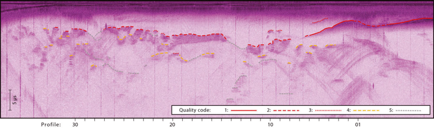
The baseband radar data were sampled at 22 MHz, and coherent integration of 25 consecutive radar records was performed using hardware on the aircraft to give an approximate spatial sampling interval of 0.2 m (assuming an aircraft speed of 60 m s -1) . Post-processing of the data consists of chirp compression followed by Doppler filtering (e.g. Reference JacksonJackson, 1986). This along-track SAR processing reduces the received power from reflections originating from fore and aft of the aircraft. However, clutter from off-axis reflectors predominately originating from locations perpendicular to the aircraft track could not be removed. It is these unwanted echoes that cause ambiguity with the desired nadir reflections from the ice base. Because of the glacier setting, it was considered operationally safer to acquire the majority of the data along the glacier and not transverse to the flow Fig. 2). The SAR data are resampled. to provide a complete record for approximately every 10 m of along-track movement and converted to SEG Y format (Reference Norris and FaichneyNorris and Faichney, 2002). Reflectors are then manually ‘picked’ using ProMAX® software. Considerable care is taken in picking all possible reflections, assigning a quality code ranging from 1 (clearly visible, continuous reflections with good contrast) to 5 (hardly visible, discontinuous reflections) to each individual reflection (Fig. 3).

Fig. 3.

Sample of post-processed RES data for the flight track highlighted in Figure 2. Vertical stripes are due to artifacts in the post-processing procedure. Reflections are classified with a quality code ranging from 1 (best quality) to 5 (poorest quality). The position of the considered cross-profiles (Fig. 8) is given.

WS 2: discarding potential side reflectors

Potential side reflectors are discarded by considering the locus of reflectors along the air-equivalent path (i.e. the distance the signal would have travelled given the echo range-time and propagation through air) of all signals (Fig. 4). If a rock wall is within a given tolerance of the air-equivalent path of a given data point, the point is discarded. The toler-zonance level is set to ±100 m, a conservative estimate which accounts for the uncertainty associated with the manual picking of individual echoes, and uncertainties in the DEM over steep topography. The application of the criteria leads to the discarding of 72% of all data points (Fig. 4a).

Fig. 4.

(a) Reflections most likely to originate from the side walls (red), and potential reflections from the glacier bed (blue; color code proportional to quality estimates). Flight tracks are shown in gray. The area in the blue rectangle is enlarged in (b). (b) Signals from side reflectors (circled in red) are identified through the envelope of the air-equivalent path for individual reflections (black circles).

WS 3: estimation of glacier bedrock and flow parameters along a first cross-profile

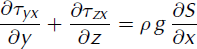
The reflections remaining after WS 2 provide a measure of the ice thickness along one cross-profile only. This profile is located 2 km upstream of the grounding line (Fig. 2). The remaining RES data alone are of insufficient quality and limited spatial coverage to allow for an area-wide estimate of ice thickness. A numerical ice-flow model designed to calculate flow velocities along cross sections of valley glaciers (Reference Sugiyama, Bauder, Zahno and FunkSugiyama and others, 2007) is therefore employed to further constrain the ice thickness distribution. In the model, the horizontal flow-speed field within a transverse profile is calculated by solving the equation for shear stress balance:

(1)

and using Glen’s flow law (Reference NyeNye, 1965):

(2)

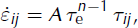
where rij and are the components of the deviatoric stress tensor and the strain rates, respectively, p the ice density, g the gravitational acceleration, S the surface elevation, A the flow rate factor, n the flow law exponent and re the effective stress. The coordinate system is defined such that x and y are along and across the flowline, respectively, and z is directed upwards. The basal flow speed, ub, is introduced as a linear function of the basal shear stress, τb, i.e.

(3)

In the model, the basal sliding coefficient, cb, is constant over the cross-profile. To solve Eqn (1), the stresses on the left-hand side are substituted by u using Eqn (2) and the relationships and . The resulting differential equation is solved for u using finite differences. Equation (3) serves as boundary condition at the base, and is implemented through a shallow, low-viscosity till layer (e.g. Reference Raymond and GudmundssonRaymond and Gudmundsson, 2005). This allows the formulation of the boundary condition at the till/bedrock interface as ‘zero velocity’, avoiding the need to prescribe individual stress components. At the surface, absence of stress is imposed. Starting from the solution of a linearly viscous flow, new effective stresses and basal flow velocity distributions are calculated from the previously determined velocity field, and the calculations repeated until the velocities converge within 10- 5 m a - 1 (Reference Sugiyama, Bauder, Zahno and FunkSugiyama and others, 2007).

The spatial resolution of the model is determined by the user, and the considered profile is discretized in 50 horizontal (i.e. across-flow) and 25 vertical nodes. Given the characteristic glacier width of 5 km, and assuming an average ice thickness of 500 m, this corresponds to a typical horizontal and vertical resolution of 100 and 20 m respectively. For the computations n is set to 3 and S/ x is determined as the median along-flow slope across the profile. The flow rate factor, A, and the basal coefficient, cb, for the first profile are determined through grid-search optimization (e.g. Reference PowellPowell, 1998; Reference LaValle, Branicky and LindemannLaValle and others, 2004), i.e. by varying the two parameters in a plausible range ([0.17, 6.8] ×10-15 s- 1 kPa-3 for A, and [0, 2] km s - 1 P a - 1 for cb, each interval subdivided into 30 steps, resulting in a total of 900 simulations) and the combination which minimizes the difference between modelled and observed surface velocity profile adopted. Comparison of modelled and observed surface velocities is performed by projecting the measured, downscaled velocities on the considered profile and linearly interpolating the two datasets to a common location. The optimization procedure yields A = 2.2×10- 1 5 s - 1 kPa-3 (a value close to that recommended for temperate ice by Reference Cuffey and PatersonCuffey and Paterson, 2010) and cb = 1.3 km s - 1 Pa - 1 (Fig. 5). The sensitivity of the model in respect to the chosen parameter combination is addressed in the section ‘Accuracy estimates’.

Fig. 5.

Grid-search optimization of parameters A and cb for profile 01 (see Fig. 8 for location). Note the logarithmic scale for A. Shading displays the average absolute deviation between modelled and observed surface velocities. The cross marks the best parameter combination. In the hatched area, the ice-flow model does not converge to any solution.

WS 4: bedrock optimization through assimilation of surface velocities

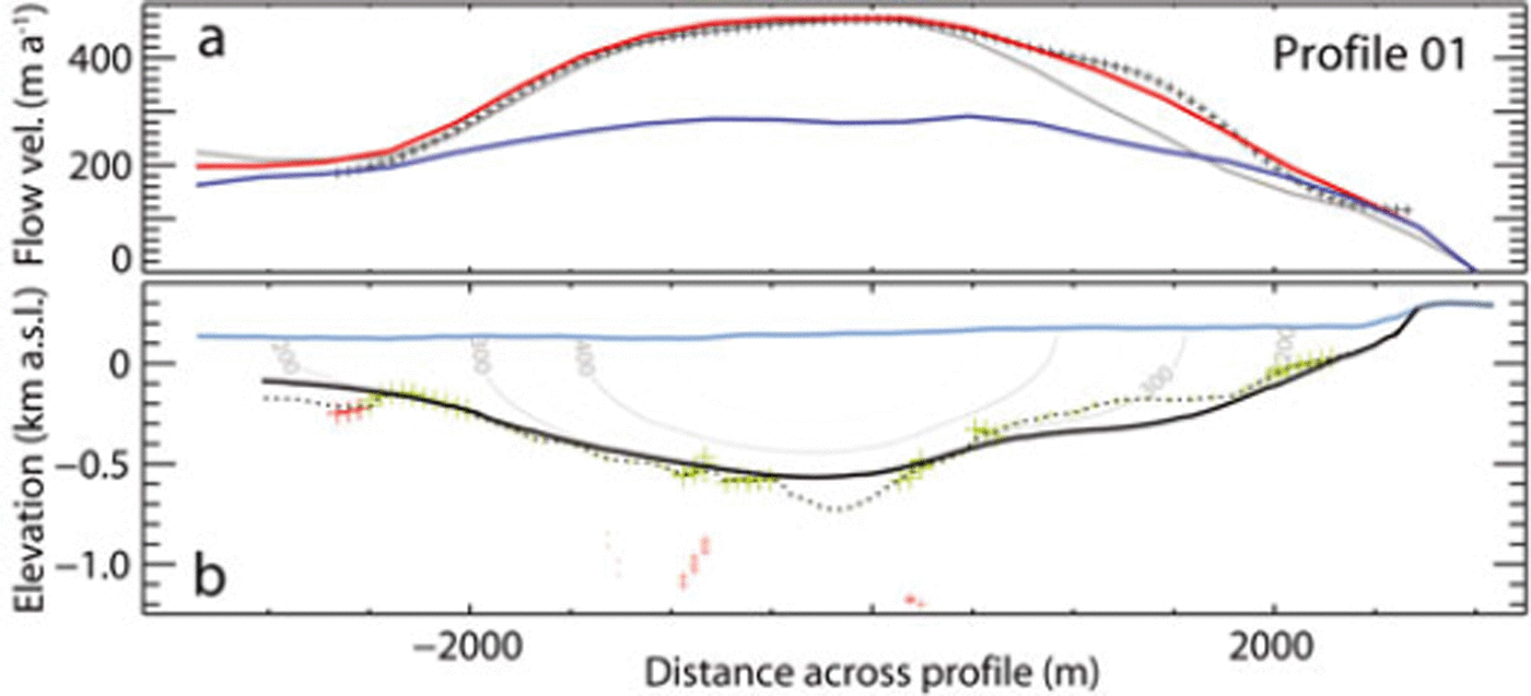
With the first estimate of the bedrock shape, the observed velocity profile at the surface cannot be reproduced in detail (Fig. 6a). In order to assimilate the data correctly, the estimated bedrock is adjusted. The adjustment is performed iteratively by updating the local estimate of the bedrock elevation according to

(4)

and recomputing the flow-velocity field for the adjusted bedrock with the ice-flow model. In Eqn (4), which was derived empirically, is the bedrock estimate for location y and iteration step i, zs,y the surface elevation at the same location, 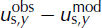the difference between observed (obs)and modelled (mod) surface velocity at y, and k an empirical coefficient set to 0.5 (a trial-and-error assessment showed this value to yield the fastest convergence rates). The updating procedure corresponds to translating half of the relative mismatch in the local surface velocity into a change in the estimated ice thickness. To ensure bedrock smoothness after adjustment, both the applied correction and the new estimate of the bedrock are filtered with a central moving average of 1/20 of the local glacier width (corresponding to ∼250 m on average). The iteration was stopped when the mean absolute relative deviation of the local surface velocity across the profile, i.e. dropped below 5%. The procedure converged within the first four (seven) iterations in the majority (all) of the cases.

Fig. 6.

Cross section for profile 01 (see Fig. 8 for location). (a) Measured (crosses) and modelled surface (red) and basal (blue) velocities for the optimized glacier bedrock, as well as for the non-optimized bedrock (gray). (b) Glacier surface (blue) and optimized bedrock (solid black). The non-optimized bedrock (dashed) follows all reflections that do not originate from the side walls (green; symbol size proportional to signal quality). The positions of echoes attributed to side reflectors are marked (red crosses). Distance across the profile is measured from the deepest point of each profile.

Ws 5: Re-Interpretation of RES Data

The optimized bedrock is used to reinterpret the reflections picked in the RES data, and the bedrock estimate adjusted accordingly (Fig. 6b). The procedure is automated by defining a deterministic correction applied locally to the bedrock. For any location, y, and any non-discarded RES reflections available, the adjusted bedrock is computed as:

(5)

with

(6)

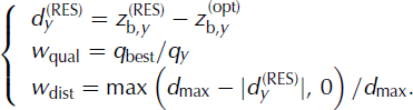
In Eqns (5) and (6), which again were derived empirically, is the adjusted bedrock elevation for location y, the elevation of the bedrock optimized through the assimilation of the surface velocities and the bedrock elevation indicated by a RES data point with assigned quality value qy. qbest stands for the best quality value assigned to any RES data point available in the considered cross-profile. Therefore, wqual is a weight for the quality values of the considered RES data point and wdist a weight for the distance between the point itself and the optimized bedrock solution. The weight, wdist, is an inverse linear function of and is set to zero for 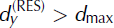(for the analyses, dmax was set to 500 m).

If, for a given location, y, multiple RES data points are available, wqual and wdist are calculated for each point individually and the bedrock adjusted according to the point with maximal combined weight. The correction for locations without RES data is calculated by smoothing the corrections for locations with data with a central moving average of 1/10 of the local glacier width. For cross-profiles without any RES data points, no such adjustment is performed.

WS 6: re-assimilation of velocity data

The adjustment of the bedrock may reintroduce a mismatch between modelled and observed surface velocities. In this case, surface velocities are reassimilated by readjusting the basal sliding coefficient, cb (Eqn (3)), of the ice-flow model (Fig. 6b). We justify the readjustment of cb on the basis that (1) WS 3 showed that the parameter is not constrained very well and (2) a spatial heterogeneity of cb appears more plausible than a heterogeneity in A, which could potentially be readjusted instead. Similarly to the optimization of the bedrock (Eqn (4)), the adjustment of cb is performed iteratively according to the relative difference between observed and modelled surface velocity:

(7)

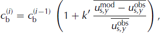
where is the updated basal coefficient at iteration step i, and mean values (e.g. ) are computed over the considered cross-profile. The empirically determined coefficient k’ was set to 2. By analogy to the bedrock optimization procedure, is used as a convergence criterion. Since cb is defined for the whole cross-profile (and not locally), the tolerance level is increased to 10% (in contrast to 5% used in WS4). Convergence was reached within six iterations for all considered profiles.

WS 7: bed estimation along additional transverse profiles and ice-flux consistency check

The output of WS5 and 6, i.e. the adjusted bedrock and the calibrated basal coefficient, are used to provide a first guess for an adjacent transverse profile located upstream. The whole optimization procedure is then repeated, starting from WS4, until enough profiles are available to interpolate a map-plane distribution of the bedrock topography.

Additionally, the integrated ice flux

(8)

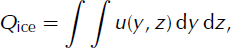
through each transverse profile is checked for mutual consistency. According to mass conservation, the difference in mass flux between two transverse profiles has to correspond to the integrated surface mass balance, rate of ice thickness change and any additional ice flux through tributaries located between the two profiles. Any transverse profile that violates this condition is omitted (Fig. 7b).

Fig. 7.

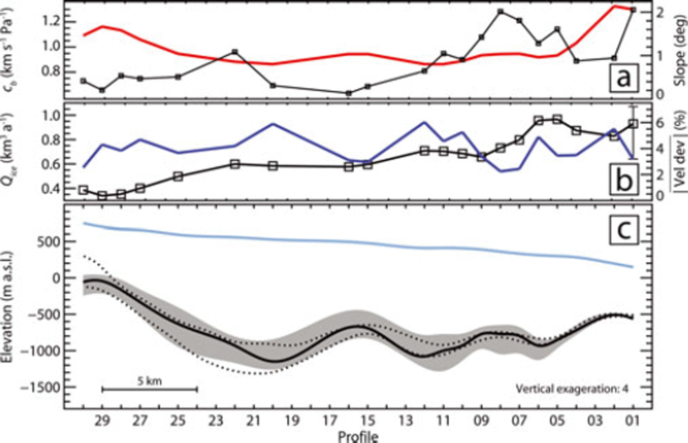
Longitudinal profile for Flask Glacier (see Fig. 8 for location). (a) Inferred basal coefficient (black) and along-flow surface slope (red). (b) Ice flux, Qice (black), and average absolute deviation between measured and modelled surface velocities (blue). For profile 01, a range is given for Qice. The lower bound assumes that the surface velocity at the profile center is given by deformation only; the upper bound assumes plug flow. In both (a) and (b), squares indicate profiles used to interpolate the final bedrock. (c) Glacier surface (blue) and glacier bedrock (black). The gray band displays the range in which the bedrock is expected, assuming randomly distributed errors. The dotted lines represent the empirical 95% confidence interval estimated for WS 8 through the resampling experiment described in the text.

In the analysis, individual profiles are spaced 1 km in the flow direction (an arbitrary choice judged to be suitable for a robust interpolation), leading to a total of 30 transverse profiles (Fig. 8).

Fig. 8.

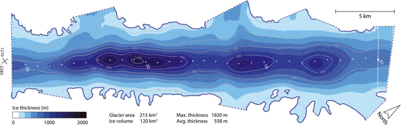
Ice thickness distribution (color map) and glacier bedrock (contours) for Flask Glacier. The deepest point of each cross-profile is given (white dots; numbers correspond to the profile name). Profile 01 is shown explicitly (dashed line), whereas all other profiles can be reconstructed from the position of the deepest points and a vector perpendicular to ice flow (flow is from left to right). The cross on the left gives a spatial reference in polar stereographic coordinates (standard parallel 7 1 • S; origin at South Pole; km).

WS 8: spatial interpolation of the glacier bedrock

The final, glacier-wide bedrock topography (Fig. 8) is obtained through a bicubic spline interpolation (Reference BhattacharyyaBhattacharyya, 1969) of the transverse profiles which are not discarded in WS 7.

Results

The resulting ice thickness distribution and the corresponding glacier bedrock topography reveal a reverse-sloped bedrock for Flask Glacier, reaching as far as 1200 m below sea level (Fig. 8; digital data retrievable at https://secure.antarctica.ac.uk/data/aerogeo/index.php). The bedrock topography corresponds mainly to a deeply incised channel and shows three distinct overdeepened areas (centered around profiles 06, 12 and 20; Fig. 7c) – a characteristic of fjord-type landscapes (e.g. Reference BirdBird, 2008; Reference Herman, Beaud, Champagnac, Lemieux and SternaiHerman and others, 2011). The total ice volume is estimated to be 120 km3, corresponding to a mean ice thickness of 560 m. Maximal ice thickness is inferred to be 1800 m.

With the final bedrock topography, measured surface velocities are accurately reproduced by the ice-flow model for every cross-profile (Figs 6 and 7b). The average point-to-point deviation is 4.2%.

The total ice discharge across the profiles drops from 0.9 km3 a - 1 near the grounding line to 0.4 km3 a - 1 for the profiles located 30 km upstream (Fig. 7b). The estimated basal slipperiness also decreases in the upstream direction (Fig. 7a). Due to the concomitant variation in basal shear stress, however, the relative contribution of basal motion to the observed surface velocity is approximately constant along the medial line (not shown). On average, basal motion contributes 6 1% (with a standard deviation of 6%) to the surface velocity observed along the medial line, with the ratio increasing towards the side margins.

Accuracy Estimates

The proposed methodology implicitly assumes that the available surface velocity field is correct, and that the ice-flow model employed is capable of describing the flow field to a sufficient accuracy. Concerning the first point, the estimated accuracy of the dataset is 10 m a - 1 (Reference Rignot, Mouginot and ScheuchlRignot and others, 2011a), whereas the flow velocity at the profile center never drops below 250 m a - 1 (Fig. 2). The maximal relative uncertainty is thus 4% and thus negligible in first instance.

Concerning the applicability of the numerical model and the robustness of its results, it is worth stating that ice velocity and ice flux are both power functions (with exponents n + 1 and n + 2, respectively) of ice thickness. Hence, relative errors in ice thickness can be expected to be (considerably) smaller than corresponding relative errors in surface velocity. Furthermore, calculated ice fluxes are rather insensitive to the exact partitioning between flow due to basal sliding and flow due to internal ice deformation. This is a consequence of the shape of the deformational profile with depth, with most of the shearing taking place in the vicinity of the bed.

To assess the sensitivity of the bedrock topography estimate to uncertainties in model parameters, the two most sensitive parameters, i.e. A and the surface slope, were changed systematically by ±10%. This sensitivity experiment suggests a lower and upper boundary for the estimated total ice volume of 105 and 135 km3, respectively, corresponding to an average ice thickness between 490 m and 630 m (Fig. 7c). The confidence intervals for the total ice volume and the average ice thickness can thus be estimated to be 120 ± 15 km3 and 560 ± 70 m, respectively. The maximal ice thickness is between 1820 and 1410 m.

Another factor influencing the shape of the calculated glacier-wide bedrock topography is the choice of the cross-profiles included in the final interpolation. Although the choice is not arbitrary, but dictated by considerations of mass conservation (WS 7), the following resampling experiment was performed. A probability of being included in the final interpolation was assigned manually to each cross-profile, based on the quality of the RES data available for the particular profile. The assigned probabilities ranged from 0.95 (95% chance of being included in the final interpolation) for profile 01 to 0.5 (equal chance of being included or not included) for profiles without any RES data, and were chosen such that the expected value for the number of included profiles corresponds to that obtained from the mass-conservation considerations (i.e. 20; Fig. 7b) had the individual profiles been selected independently from a set of binomial distributions. The selection of a set of cross-profiles and the interpolation of a final bedrock topography was then performed 1000 times. The 2.5% and 97.5% quantiles of the so obtained empirical probability distribution for the bedrock topography are shown in Figure 7c, providing an empirical 95% confidence interval for that particular working step. On that basis, the uncertainty introduced in the mean ice thickness through the choice of the profiles can be estimated to be on the order of ±100 m.

The calculated ice volume flux, Qice, is dependent on assumptions made about basal sliding. To estimate the sensitivity of our results to different assumptions about sliding, two end members were considered for profile 0 1 . The first assumes plug flow across the profile (i.e. uy(z) = us,y for every z and given y), the second that the surface velocity observed at the profile center is entirely due to ice deformation (i.e. ub,y = 0 for every y). The two end members provide an upper and a lower bound for Qice corresponding to [1.07, 0.64] km3 a - 1 , i.e. [+15%, -31%] compared to the best estimate (Fig. 7b). This can be considered the level to which Qice is known along the longitudinal profile. It must be noted that through the assimilation of the surface velocities the contributions to Qice from the lateral glacier branches merging with the main glacier trunk are accounted for implicitly and not neglected.

Conclusions

A glacier-wide bedrock topography was derived for Flask Glacier by assimilating observed surface velocities and sparse and uncertain RES data within an ice-flow model. The accuracy of the bedrock estimate was assessed by performing a sensitivity study on the parameters of the ice-flow model and through a resampling experiment.

The derived total ice volume for Flask Glacier is 120 ± 15 km3, corresponding to an average ice thickness of 560 ± 70 m. Almost the entire length of the glacier bed is below sea level, and the maximal inferred ice thickness is between 1410 and 1820 m. The upper bound on thickness places the deepest parts of the bedrock 1200 m below sea level.

Although the specific geometry of Flask Glacier makes it particularly suited for the application of the approach presented, the developed methodology could be applied to other glaciers where surface velocities are available. A precondition is that the glacier bedrock can be determined, with a sufficient degree of confidence, for at least one cross section.