


Impact Statement
In scientific machine learning, trusted metrics (e.g., object counting) are often non-differentiable, breaking the gradient signal required for training. Consequently, models rely on smooth proxies (like mean-squared error) and underperform on scientific validation. We provide a solution via a “differentiable surrogate”: a secondary neural network that mimics these metrics. By embedding strict rules, we ensure the surrogate provides stable, valid feedback. While demonstrated on weather radar data to enforce storm geometry, this framework allows researchers in any field (i.e., weather downscaling, wildfire segmentation, and ocean eddy detection) to train models directly with gold-standard domain metrics.
1. Introduction
Structural realism in predicted precipitation fields depends on metrics that are inherently non-differentiable, creating a bottleneck for gradient-based optimization. To bridge this gap, we leverage knowledge from integral geometry, which reveals organizational biases often missed by standard statistical verification. Unlike recent work exploring surrogates in latent spaces (Patel et al., Reference Patel, Hodan and Matas2020), we enforce these properties directly in the optimization landscape. We introduce a framework situated at the intersection of differentiable programming (Gelbrecht et al., Reference Gelbrecht, White, Bathiany and Boers2023) and knowledge-guided machine learning (Karpatne et al., Reference Karpatne, Atluri, Faghmous and Kumar2017) (Figure 1). Within this framework, we compare an analytical approximation against a neural emulator, both designed to map the level sets of precipitation fields to key integral-geometric measures (area, perimeter, and number of connected components). By relaxing this discrete combinatorial problem into a continuous regression task (Hu et al., Reference Hu, Li, Samaras and Chen2019), we enable the direct backpropagation of structural error signals. Crucially, we ensure emulation stability by adopting a knowledge-guided Lipschitz-Convolutional Neural Network (Lip-CNN) (Gouk et al., Reference Gouk, Frank, Pfahringer and Cree2021). This architecture combines spectral normalization—to prevent exploding gradients—with hard geometric constraints (monotonicity and isoperimetry) embedded in the computation graph.
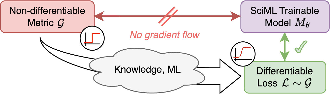
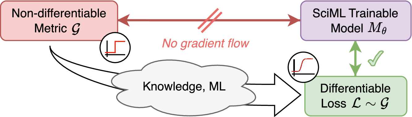
Conceptual overview of the differentiable surrogate training framework. The lack of gradient flow (red connection) prevents the direct optimization of SciML models (
$ {M}_{\theta } $
 ) using non-differentiable scientific metrics (
$ \mathcal{G} $
) using non-differentiable scientific metrics (
$ \mathcal{G} $
 ), which typically involve discrete operations like thresholding (step function plot). We overcome this limitation by using knowledge and machine learning techniques to create a differentiable surrogate loss (
$ \mathrm{\mathcal{L}} $
), which typically involve discrete operations like thresholding (step function plot). We overcome this limitation by using knowledge and machine learning techniques to create a differentiable surrogate loss (
$ \mathrm{\mathcal{L}} $
 ) that approximates the target metric. This differentiable loss, with a well-behaved optimization landscape, can then be successfully integrated into the model’s training pipeline (green connection), enabling the direct backpropagation of structurally and physically relevant error signals.
Concurrent efforts to integrate non-differentiable operations into automatic differentiation frameworks, such as the SoftJAX and SoftTorch libraries (Paulus et al., Reference Paulus, Geist, Musil, Hoffmann, Beker and Martius2026), provide general-purpose continuous relaxations for elemental primitives (e.g., thresholding and fuzzy logic). While these drop-in replacements facilitate the formulation of analytical approximations akin to our continuous baseline, cascading numerous element-wise soft operators through complex topological algorithms frequently exacerbates gradient attenuation and mathematical entanglement. In contrast, our Lipschitz-regularized neural emulation circumvents the need for explicit operator relaxation by learning a holistic, topologically informed mapping that ensures robust structural fidelity and stable gradient flow.
Our primary contributions are: (1) proposing a general framework for injecting non-differentiable domain knowledge into training via learned surrogates, compared against standard analytical approximations; (2) introducing the Minkowski image loss, a differentiable objective that penalizes errors in rigid-motion invariants (area, perimeter, and connected components); and (3) demonstrating that hard geometric constraints paired with Lipschitz regularization prevents violating geometric principles and overfitting observed in unconstrained baselines.
2. Methodology
2.1. Approaches to non-differentiable metrics
Scientific evaluation often relies on functionals
$ f:\mathcal{X}\to \mathcal{Y} $
 involving discrete operations such as counting, thresholding, or binning. These operations are inherently non-differentiable; they manifest as piecewise constant functions whose gradient
$ {\nabla}_{\mathbf{x}}f $
involving discrete operations such as counting, thresholding, or binning. These operations are inherently non-differentiable; they manifest as piecewise constant functions whose gradient
$ {\nabla}_{\mathbf{x}}f $
 is zero almost everywhere or undefined at jump discontinuities (Dirac deltas), producing a loss surface of flat plateaus that prevents the backpropagation of error signals required to update an upstream model. Two primary methodologies exist to circumvent this limitation. The first relies on analytical approximation, wherein discrete operations are substituted with continuous, smooth relaxations, yielding a closed-form differentiable surrogate. The second leverages neural emulation, employing an artificial neural network to map the input space directly to the target metric; because neural networks are differentiable by construction, this learned surrogate integrates seamlessly into the computational graph.
2.1.1. Analytical approximation of non-differentiable metrics
The analytical approximation strategy aims to replace non-differentiable operations with smooth variants that permit stable gradient flow. For example, binary thresholding—mathematically represented by the Heavisine step function
$ H(x) $
 —is commonly relaxed using a logistic sigmoid function
$ \sigma \left(x/\tau \right) $
—is commonly relaxed using a logistic sigmoid function
$ \sigma \left(x/\tau \right) $
 . Here,
$ \tau >0 $
. Here,
$ \tau >0 $
 acts as a temperature parameter controlling the steepness of the approximation. As
$ \tau \to 0 $
acts as a temperature parameter controlling the steepness of the approximation. As
$ \tau \to 0 $
 , the continuous function converges to the exact discrete behavior, but its gradients vanish almost everywhere; conversely, larger values of
$ \tau $
, the continuous function converges to the exact discrete behavior, but its gradients vanish almost everywhere; conversely, larger values of
$ \tau $
 provide stable gradients at the cost of approximation fidelity. Consequently,
$ \tau $
provide stable gradients at the cost of approximation fidelity. Consequently,
$ \tau $
 is often annealed dynamically during optimization. Similar continuous relaxations are employed for discrete selection operations, such as replacing
$ \arg \max $
is often annealed dynamically during optimization. Similar continuous relaxations are employed for discrete selection operations, such as replacing
$ \arg \max $
 with a differentiable softmax approximation (Jang et al., Reference Jang, Gu and Poole2017). While these analytical substitutions preserve the mechanistic interpretability of the original metric, deriving stable, closed-form relaxations for complex, multistep spatial metrics is not always mathematically possible.
2.1.2. Emulation of non-differentiable metrics: Surrogate modeling and Lipschitz regularization
To restore differentiability, we approximate the discrete map
$ f $
 with a parameterized neural surrogate
$ {f}_{\theta }:\mathcal{X}\to \mathcal{Y} $
with a parameterized neural surrogate
$ {f}_{\theta }:\mathcal{X}\to \mathcal{Y} $
 . Minimizing the regression error on static data is insufficient: For
$ {f}_{\theta } $
. Minimizing the regression error on static data is insufficient: For
$ {f}_{\theta } $
 to serve as a stable loss function, it must provide “well-behaved” gradients that are informative across the input domain
$ \mathcal{D} $
to serve as a stable loss function, it must provide “well-behaved” gradients that are informative across the input domain
$ \mathcal{D} $
 .
.
Gradient propagation: A critical requirement is nonvanishing input sensitivity. To avoid the “dead zones” associated with rectifying activations (e.g., ReLU, where
$ \nabla =0 $
 for
$ x<0 $
for
$ x<0 $
 ), we employ smooth,
$ {C}^{\infty } $
), we employ smooth,
$ {C}^{\infty } $
 activation functions—specifically the Gaussian Error Linear Unit (GELU; Hendrycks and Gimpel, Reference Hendrycks and Gimpel2016). Furthermore, to facilitate gradient flow through deep architectures, we utilize residual connections
$ \mathbf{y}=\mathbf{x}+F\left(\mathbf{x}\right) $
activation functions—specifically the Gaussian Error Linear Unit (GELU; Hendrycks and Gimpel, Reference Hendrycks and Gimpel2016). Furthermore, to facilitate gradient flow through deep architectures, we utilize residual connections
$ \mathbf{y}=\mathbf{x}+F\left(\mathbf{x}\right) $
 , allowing error signals to propagate unimpeded through the identity path.
Manifold smoothing: Early in training, the upstream model may yield a distribution
$ {P}_{\mathrm{g}} $
 far from the data distribution
$ {P}_{\mathrm{data}} $
far from the data distribution
$ {P}_{\mathrm{data}} $
 ; if trained only on
$ {P}_{\mathrm{data}} $
; if trained only on
$ {P}_{\mathrm{data}} $
 ’s support, the emulator can yield arbitrary gradients for
$ \mathbf{x}\sim {P}_{\mathrm{g}} $
’s support, the emulator can yield arbitrary gradients for
$ \mathbf{x}\sim {P}_{\mathrm{g}} $
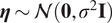
 . We hence inject Gaussian noise
$ \boldsymbol{\eta} \sim \mathcal{N}\left(\mathbf{0},{\sigma}^2\mathbf{I}\right) $
. We hence inject Gaussian noise
$ \boldsymbol{\eta} \sim \mathcal{N}\left(\mathbf{0},{\sigma}^2\mathbf{I}\right) $
 during emulator training, effectively convolving the target functional with a smoothing kernel and improving robustness to off-manifold queries. (In practice, we found this step unnecessary for the OPERA dataset, given the Mix-Up augmentation described in Section 3.1, and set
$ {\sigma}^2=0 $
during emulator training, effectively convolving the target functional with a smoothing kernel and improving robustness to off-manifold queries. (In practice, we found this step unnecessary for the OPERA dataset, given the Mix-Up augmentation described in Section 3.1, and set
$ {\sigma}^2=0 $
 in all reported experiments.)
Lipschitz constraints: Finally, we bound the gradient norm to prevent optimization instability. Unconstrained neural networks can learn arbitrarily sharp gradients, leading to exploding loss terms. We enforce stability by constraining the Lipschitz constant
$ K $
 of the network mapping. While soft constraints like the gradient penalty (Gulrajani et al., Reference Gulrajani, Ahmed, Arjovsky, Dumoulin and Courville2017) are common in adversarial training, they do not guarantee bounds on unseen data. Instead, we enforce a hard constraint via spectral normalization (Miyato et al., Reference Miyato, Kataoka, Koyama and Yoshida2018) on all weight matrices
$ {W}_l $
of the network mapping. While soft constraints like the gradient penalty (Gulrajani et al., Reference Gulrajani, Ahmed, Arjovsky, Dumoulin and Courville2017) are common in adversarial training, they do not guarantee bounds on unseen data. Instead, we enforce a hard constraint via spectral normalization (Miyato et al., Reference Miyato, Kataoka, Koyama and Yoshida2018) on all weight matrices
$ {W}_l $
 . This ensures that the global Lipschitz constant is bounded by the product of the layer-wise spectral norms:
$ \parallel {f}_{\theta}\left(\mathbf{x}\right)-{f}_{\theta}\left(\mathbf{y}\right){\parallel}_2\le K\parallel \mathbf{x}-\mathbf{y}{\parallel}_2 $
. This ensures that the global Lipschitz constant is bounded by the product of the layer-wise spectral norms:
$ \parallel {f}_{\theta}\left(\mathbf{x}\right)-{f}_{\theta}\left(\mathbf{y}\right){\parallel}_2\le K\parallel \mathbf{x}-\mathbf{y}{\parallel}_2 $
 , implying
$ {\sup}_{\mathbf{x}\in \mathcal{D}}\parallel {\nabla}_{\mathbf{x}}{f}_{\theta}\left(\mathbf{x}\right){\parallel}_2\le K $
, implying
$ {\sup}_{\mathbf{x}\in \mathcal{D}}\parallel {\nabla}_{\mathbf{x}}{f}_{\theta}\left(\mathbf{x}\right){\parallel}_2\le K $
 , almost everywhere in
$ \mathcal{D} $
, almost everywhere in
$ \mathcal{D} $
 , where typically
$ K\approx 1 $
, where typically
$ K\approx 1 $
 and
$ \parallel .{\parallel}_2 $
and
$ \parallel .{\parallel}_2 $
 is the
$ {L}^2 $
is the
$ {L}^2 $
 norm. While fixing
$ K $
norm. While fixing
$ K $
 before training limits the network’s expressivity if the true functional varies rapidly (Ducotterd et al., Reference Ducotterd, Goujon, Bohra, Campos and Unser2022), for the integral-geometric measures considered in Section 2.2, empirical results suggest that the stability benefits of a hard
$ K=1 $
before training limits the network’s expressivity if the true functional varies rapidly (Ducotterd et al., Reference Ducotterd, Goujon, Bohra, Campos and Unser2022), for the integral-geometric measures considered in Section 2.2, empirical results suggest that the stability benefits of a hard
$ K=1 $
 constraint outweighs the theoretical expressivity loss.
2.2. Minkowski image loss: Injecting knowledge from integral geometry
2.2.1. Integral-geometric characterization via Minkowski functionals
To capture the structural properties of physical fields beyond pixel-wise intensity, we adopt a framework based on the Minkowski functionals from integral geometry (Schneider and Weil, Reference Schneider and Weil2008). For a compact set
$ K\subset {\unicode{x211D}}^2 $
 with a sufficiently smooth boundary (see Supplementary Appendix A), there exist three Minkowski functionals: the area, half the perimeter, and the Euler characteristic. These functionals are denoted
$ {A}_K $
with a sufficiently smooth boundary (see Supplementary Appendix A), there exist three Minkowski functionals: the area, half the perimeter, and the Euler characteristic. These functionals are denoted
$ {A}_K $
 ,
$ {P}_{K/2} $
,
$ {P}_{K/2} $
 , and
$ {\chi}_K $
, and
$ {\chi}_K $
 , respectively. The Euler characteristic describes the connectivity of the set and is defined in 2D as
$ {\chi}_K={\mathrm{CC}}_K-{H}_K $
, respectively. The Euler characteristic describes the connectivity of the set and is defined in 2D as
$ {\chi}_K={\mathrm{CC}}_K-{H}_K $
 , where
$ {\mathrm{CC}}_K $
, where
$ {\mathrm{CC}}_K $
 is the number of connected components and
$ {H}_K $
is the number of connected components and
$ {H}_K $
 is the number of holes. The suitability of these measures for a loss function is rigorously grounded in Hadwiger’s Characterization Theorem (Hadwiger, Reference Hadwiger1957), which establishes that any functional on
$ K $
is the number of holes. The suitability of these measures for a loss function is rigorously grounded in Hadwiger’s Characterization Theorem (Hadwiger, Reference Hadwiger1957), which establishes that any functional on
$ K $
 satisfying rigid-motion invariance, continuity, and additivity can be expressed as a linear combination of these three measures. These mathematical properties map directly to critical advantages in neural network training: (i) Rigid-motion invariance: Decouples the loss from the exact spatial positioning of extreme events, mitigating the “double penalty” problem (Ebert, Reference Ebert2008) inherent in pixel-wise metrics where a slight displacement is penalized twice (as a miss and a false alarm). (ii) Continuity: Ensures gradient stability, as minor shape deformations result in commensurate, small changes in the loss value, unlike discontinuous metrics (e.g., pure object counting), which exhibit step functions.
2.2.2. The
$ \gamma $
 -vector and Minkowski image loss formulation

A continuous physical field is transformed into
$ N $
 binary images (excursion sets) by thresholding at
$ N $
binary images (excursion sets) by thresholding at
$ N $
 intensity levels,
$ {u}^{(1)},\dots, {u}^{(N)} $
intensity levels,
$ {u}^{(1)},\dots, {u}^{(N)} $
 . For each excursion set, we compute the area (
$ A $
. For each excursion set, we compute the area (
$ A $
 ), perimeter (
$ P $
), perimeter (
$ P $
 ), and the number of connected components (
$ \mathrm{CC} $
), and the number of connected components (
$ \mathrm{CC} $
 ). The values of these functionals for the
$ i $
). The values of these functionals for the
$ i $
 -th threshold are denoted
$ {A}^{(i)} $
-th threshold are denoted
$ {A}^{(i)} $
 ,
$ {P}^{(i)} $
,
$ {P}^{(i)} $
 , and
$ {\mathrm{CC}}^{(i)} $
, and
$ {\mathrm{CC}}^{(i)} $
 . We concatenate these statistics into a single nonnegative vector
$ \boldsymbol{\gamma} $
. We concatenate these statistics into a single nonnegative vector
$ \boldsymbol{\gamma} $
 that provides a multilevel integral-geometric summary of the field:

The distance between two
$ \boldsymbol{\gamma} $
 -vectors serves as a proxy for the structural divergence between the predicted and target fields. Integrating this metric into training ensures the network minimizes geometric error alongside pixel-wise error. The reader is referred to Supplementary Appendix B.2 for further details regarding the computation of the
$ \gamma $
-vectors serves as a proxy for the structural divergence between the predicted and target fields. Integrating this metric into training ensures the network minimizes geometric error alongside pixel-wise error. The reader is referred to Supplementary Appendix B.2 for further details regarding the computation of the
$ \gamma $
 -vector from data.
A significant challenge is the order-of-magnitude disparity between vector components;
$ {A}^{(i)} $
 (pixel summation) can be orders of magnitude larger than
$ {\mathrm{CC}}^{(i)} $
(pixel summation) can be orders of magnitude larger than
$ {\mathrm{CC}}^{(i)} $
 (sparse count). Without normalization, gradients would be dominated by area terms, ignoring topological structure. To address this, we define the Minkowski image loss
$ \mathcal{M} $
(sparse count). Without normalization, gradients would be dominated by area terms, ignoring topological structure. To address this, we define the Minkowski image loss
$ \mathcal{M} $
 using a log-transformed
$ {L}^1 $
using a log-transformed
$ {L}^1 $
 distance. This transformation effectively normalizes the scale differences, operating as a relative error metric that balances the contribution of large-magnitude features (area) and small-magnitude features (connectivity):

where
$ \mathbf{1} $
 is a vector of ones to ensure numerical stability and
$ \parallel .{\parallel}_1 $
is a vector of ones to ensure numerical stability and
$ \parallel .{\parallel}_1 $
 is the
$ {L}^1 $
is the
$ {L}^1 $
 norm. This Minkowski image loss functions as a regularizer alongside standard pixel-wise metrics (e.g., MSE). While pixel loss enforces local intensity accuracy,
$ \mathcal{M} $
norm. This Minkowski image loss functions as a regularizer alongside standard pixel-wise metrics (e.g., MSE). While pixel loss enforces local intensity accuracy,
$ \mathcal{M} $
 acts as a global structural constraint. Since the direct computation of
$ \boldsymbol{\gamma} $
acts as a global structural constraint. Since the direct computation of
$ \boldsymbol{\gamma} $
 involves non-differentiable operations (thresholding and counting) that break the computation graph, we employ the knowledge-guided differentiable surrogate described in Section 2.1. This surrogate allows the error signal
$ {\nabla}_{\hat{\boldsymbol{\gamma}}}\mathcal{M} $
involves non-differentiable operations (thresholding and counting) that break the computation graph, we employ the knowledge-guided differentiable surrogate described in Section 2.1. This surrogate allows the error signal
$ {\nabla}_{\hat{\boldsymbol{\gamma}}}\mathcal{M} $
 to be backpropagated through the emulator to update the trainable model.
2.3. Application to integral-geometric measures
While analytical approximations directly relax discrete metrics, formulating closed-form solutions for complex topologies proves computationally restrictive and prone to vanishing gradients. As a robust alternative, we introduce a neural emulator as a learned differentiable surrogate, approximating the non-differentiable mapping
$ F:\mathcal{X}\to {\unicode{x211D}}^{3N} $
 from physical fields to
$ \boldsymbol{\gamma} $
from physical fields to
$ \boldsymbol{\gamma} $
 -vectors. Standard pixel-wise metrics (e.g., MSE) inherently smooth the multiscale spatial organization critical to precipitation modeling. By embedding this emulator into the loss function, we directly penalize geometric errors. We train the model to regress exact ground-truth descriptors (area, perimeter and connected components) generated via GUDHI (Maria et al., Reference Maria, Boissonnat, Glisse and Yvinec2014). The bipartite architecture pairs a Lipschitz-regularized feature extractor with geometrically constrained heads to decode valid
$ \boldsymbol{\gamma} $
-vectors. Standard pixel-wise metrics (e.g., MSE) inherently smooth the multiscale spatial organization critical to precipitation modeling. By embedding this emulator into the loss function, we directly penalize geometric errors. We train the model to regress exact ground-truth descriptors (area, perimeter and connected components) generated via GUDHI (Maria et al., Reference Maria, Boissonnat, Glisse and Yvinec2014). The bipartite architecture pairs a Lipschitz-regularized feature extractor with geometrically constrained heads to decode valid
$ \boldsymbol{\gamma} $
 -vector components.
2.3.1. Analytical approximation of integral-geometric measures
Our analytical approximation substitutes the non-differentiable Heaviside step function with a temperature-controlled sigmoid, mapping the continuous physical field into a pseudo-probability space
$ P\in \left(0,1\right) $
 to enable differentiable tensor operations. We calculate the area as the weighted sum of
$ P $
to enable differentiable tensor operations. We calculate the area as the weighted sum of
$ P $
 and derive perimeter from finite-difference approximations of spatial derivatives. To compute the Euler characteristic (a proxy for connected components), we evaluate the alternating sum of grid vertices, edges, and faces, replacing discrete boolean logic with the Gödel t-norm (min operator) to ensure continuous gradient flow. To stabilize these topological metrics against minor fluctuations, we preprocess the input tensor using differentiable morphological filters and a local persistence threshold mask, ultimately aggregating and scaling the measures via a symmetric logarithm.
2.3.2. Emulation of integral-geometric measures via knowledge-guided learning
Feature extractor with Lip-CNN.
To map the physical field
$ \mathbf{x}\in {\unicode{x211D}}^{H\times W} $
 to the latent geometric manifold
$ \mathbf{z} $
to the latent geometric manifold
$ \mathbf{z} $
 , we employ a CNN encoder designed to respect the mathematical constraints of the
$ \boldsymbol{\gamma} $
, we employ a CNN encoder designed to respect the mathematical constraints of the
$ \boldsymbol{\gamma} $
 -vector. The input field is normalized to
$ \left[0,1\right] $
-vector. The input field is normalized to
$ \left[0,1\right] $
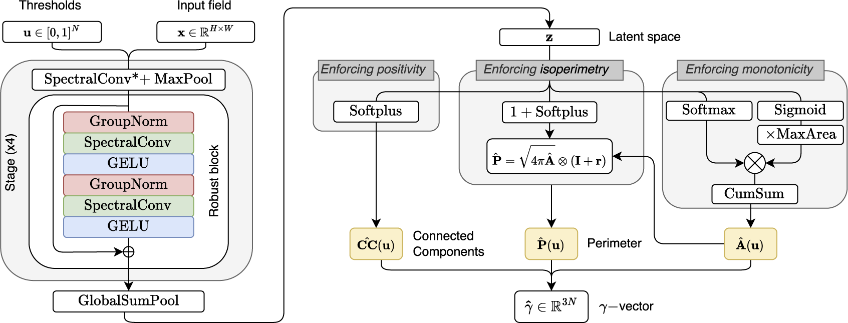
 via a fixed scaling factor. The backbone processes the field through four hierarchical stages (Figure 2, left), with spectral normalization (Miyato et al., Reference Miyato, Kataoka, Koyama and Yoshida2018) applied to all convolutional kernels except the first layer, which is left unconstrained to allow unrestricted input scaling. Deep feature extraction is handled by “robust blocks” containing residual connections and group normalization, ensuring invariance to batch statistics. We use global sum pooling rather than average pooling, since area and connected components are extensive quantities whose additivity must be preserved as the latent representation scales with domain size.
(Left) Lipschitz-bound feature extractor: The backbone acts as a hierarchical encoder. Stability is enforced via spectral normalization and residual connections. We use global sum pooling to preserve the extensivity of geometric features. (Right) Geometric constraint heads: The area
$ \hat{A}(u) $
 is constructed via integration of a predicted probability density to enforce monotonicity. The perimeter
$ \hat{P}(u) $
is constructed via integration of a predicted probability density to enforce monotonicity. The perimeter
$ \hat{P}(u) $
 is conditioned on the area via the isoperimetric inequality, preventing geometric principles’ violations.
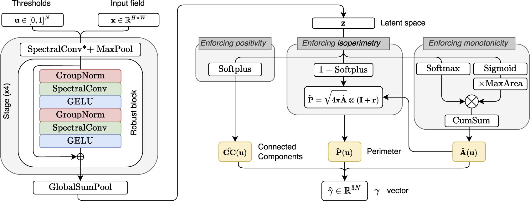
Figure 2. Long description
The diagram consists of two main sections connected by a flow arrow.
Left Panel: Lipschitz-bound feature extractor.
* At the top, two inputs are defined: Thresholds u in [0, 1] super N and Input field x in R super H times W.
* These feed into a Spectral Conv asterisk plus Max Pool layer.
* Below this is a Robust block labeled Stage (x4). It contains a vertical stack of layers: Group Norm, Spectral Conv, GEL U, followed by a second set of Group Norm, Spectral Conv, and GELU. A residual connection bypasses these layers to a plus symbol at the bottom.
* The output of the stage enters a Global Sum Pool layer.
Right Panel: Geometric constraint heads.
* An arrow from the left panel leads to a Latent space vector z.
* Vector z branches into three parallel modules:
1. Enforcing positivity: A Softplus layer leads to CC hat (u) representing Connected Components.
2. Enforcing isoperimetry: A 1 plus Softplus layer feeds into an equation box: P hat equals square root of 4 pi A hat times (I plus r). This outputs P hat (u) representing Perimeter.
3. Enforcing monotonicity: A Softmax layer and a Sigmoid layer (multiplied by Max Area) feed into a multiplication symbol, followed by a Cum Sum layer. This outputs A hat (u) representing Area.
* The Area output A hat (u) also feeds back into the isoperimetry equation.
* All three outputs (Connected Components, Perimeter, and Area) converge at the bottom into a final gamma-vector: gamma hat in R super 3 N.
Knowledge-guided geometric constraints. Unlike standard multi-task regression, where outputs are independent, our architecture couples the output heads to strictly enforce geometric consistency.
Area head (monotonicity via integration). Directly regressing the area metric
$ {A}^{(i)} $
 for each threshold fails to guarantee the monotonicity property
$ {A}^{(i)}\ge {A}^{\left(i+1\right)} $
for each threshold fails to guarantee the monotonicity property
$ {A}^{(i)}\ge {A}^{\left(i+1\right)} $
 (as threshold increases, excursion set area decreases). To resolve this, we use the fact that the area function is effectively the cumulative distribution function of the field intensities. The network predicts a discrete probability density using a softmax layer and a scalar total area
$ {A}_{\mathrm{total}} $
(as threshold increases, excursion set area decreases). To resolve this, we use the fact that the area function is effectively the cumulative distribution function of the field intensities. The network predicts a discrete probability density using a softmax layer and a scalar total area
$ {A}_{\mathrm{total}} $
 . The final area vector
$ \hat{\mathbf{A}} $
. The final area vector
$ \hat{\mathbf{A}} $
 is computed via the cumulative sum of these probabilities. This inductive bias ensures that the predicted area is strictly monotonic by construction.
Perimeter head (isoperimetric inequality). We strictly condition the perimeter on the area by predicting a dimensionless “roughness” coefficient
$ \hat{\mathbf{r}}\ge 0 $
 (via a Softplus activation) rather than the absolute perimeter. The perimeter is then reconstructed as
$ \hat{\mathbf{P}}=\sqrt{4\pi \hat{\mathbf{A}}}\odot \left(\mathbf{1}+\hat{\mathbf{r}}\right) $
(via a Softplus activation) rather than the absolute perimeter. The perimeter is then reconstructed as
$ \hat{\mathbf{P}}=\sqrt{4\pi \hat{\mathbf{A}}}\odot \left(\mathbf{1}+\hat{\mathbf{r}}\right) $
 . This hard-codes the isoperimetric inequality (
$ {P}^2\ge 4\pi A $
. This hard-codes the isoperimetric inequality (
$ {P}^2\ge 4\pi A $
 ) into the forward pass. It prevents the model from generating a perimeter smaller than that of a perfect circle with equivalent area, ensuring 0% geometrical violations.
Topological head (positivity). The number of connected components
$ \mathrm{CC} $
 is a counting measure. To reflect this, the output is rectified using Softplus (
$ \log \left(1+{e}^x\right) $
is a counting measure. To reflect this, the output is rectified using Softplus (
$ \log \left(1+{e}^x\right) $
 ), ensuring
$ \hat{\mathrm{CC}}\in {\unicode{x211D}}_{+} $
), ensuring
$ \hat{\mathrm{CC}}\in {\unicode{x211D}}_{+} $
 while maintaining differentiable nonzero gradients, unlike a hard ReLU clip, which may lead to “dead neurons”.
Training setup.
Motivated by the target data’s statistical properties, we optimize
$ \theta $
 using the Minkowski image loss:
$ {\mathrm{\mathcal{L}}}_{\mathrm{train}}=\mathcal{M}\left({\hat{\boldsymbol{\gamma}}}_{\theta}\left(\mathbf{x}\right),{\boldsymbol{\gamma}}_{\mathrm{true}}\right) $
using the Minkowski image loss:
$ {\mathrm{\mathcal{L}}}_{\mathrm{train}}=\mathcal{M}\left({\hat{\boldsymbol{\gamma}}}_{\theta}\left(\mathbf{x}\right),{\boldsymbol{\gamma}}_{\mathrm{true}}\right) $
 . Logarithmic scaling prevents large disparities between area and connected components, while the
$ {L}^1 $
. Logarithmic scaling prevents large disparities between area and connected components, while the
$ {L}^1 $
 norm ensures stability against outliers from complex storm structures.
3. Application: Observed instantaneous surface precipitation fields
Emulating Minkowski functionals is particularly relevant for precipitation, which—unlike smooth fields—exhibits high intermittency, non-Gaussian statistics, and complex multiscale geometries. Standard pixel-wise losses often fail to capture these morphological properties, leading to structurally amorphous (“blurred”) predictions. By applying our Minkowski image loss to radar-based precipitation estimates, we aim to encourage realistic structures in generative tasks, specifically km-scale downscaling.
3.1. Dataset and preprocessing
We validate our approach using the pan-European EUMETNET radar composites provided by the European Operational Program for Exchange of Weather Radar Information (OPERA) (Saltikoff et al., Reference Saltikoff, Haase, Delobbe, Gaussiat, Martet, Idziorek, Leijnse, Novák, Lukach and Stephan2019). We utilize the instantaneous surface rain rate product, leveraging high-definition streams (ODISSEY/NIMBUS) with 15-minute updates. Spanning August 1, 2023, to October 30, 2024, this archive yields >1M patches of 128
$ \times $
 128 pixels (256
$ \times $
128 pixels (256
$ \times $
 256 km) across diverse regimes, from localized summer convection to large-scale winter synoptic storms. We partition the dataset chronologically to preclude temporal autocorrelation: data from August 2023 through June 2024 is utilized for training, July 2024 for validation, and August through October 2024 is reserved for independent testing. We apply a drizzle threshold
$ \delta =0.1\;\mathrm{mm}\;{\mathrm{h}}^{-1} $
256 km) across diverse regimes, from localized summer convection to large-scale winter synoptic storms. We partition the dataset chronologically to preclude temporal autocorrelation: data from August 2023 through June 2024 is utilized for training, July 2024 for validation, and August through October 2024 is reserved for independent testing. We apply a drizzle threshold
$ \delta =0.1\;\mathrm{mm}\;{\mathrm{h}}^{-1} $
 ; intensity values below
$ \delta $
; intensity values below
$ \delta $
 are zeroed out to remove sensor noise. For training, data undergoes a log-linear transformation to compress the dynamic range:
$ {x}_{\mathrm{norm}}=\log \left(1+x\right)/S $
are zeroed out to remove sensor noise. For training, data undergoes a log-linear transformation to compress the dynamic range:
$ {x}_{\mathrm{norm}}=\log \left(1+x\right)/S $
 , where
$ S $
, where
$ S $
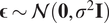
 is the global maximum of the log-transformed training set. To enforce robustness, we apply an offline “Mix-Up” strategy in physical space. We generate synthetic convex combinations of ground truth fields and noise-injected interpolated fields to ensure off-manifold robustness:
$ {\mathbf{x}}_{\mathrm{mix}}=\lambda {\mathbf{x}}_{\mathrm{real}}+\left(1-\lambda \right)\left({\mathbf{x}}_{\mathrm{interp}}+\boldsymbol{\unicode{x025B}} \right) $
is the global maximum of the log-transformed training set. To enforce robustness, we apply an offline “Mix-Up” strategy in physical space. We generate synthetic convex combinations of ground truth fields and noise-injected interpolated fields to ensure off-manifold robustness:
$ {\mathbf{x}}_{\mathrm{mix}}=\lambda {\mathbf{x}}_{\mathrm{real}}+\left(1-\lambda \right)\left({\mathbf{x}}_{\mathrm{interp}}+\boldsymbol{\unicode{x025B}} \right) $
 where
$ \lambda \sim \mathrm{Beta}\left(\alpha, \alpha \right) $
where
$ \lambda \sim \mathrm{Beta}\left(\alpha, \alpha \right) $
 and
$ \boldsymbol{\unicode{x025B}} \sim \mathcal{N}\left(\mathbf{0},{\sigma}^2\mathbf{I}\right) $
and
$ \boldsymbol{\unicode{x025B}} \sim \mathcal{N}\left(\mathbf{0},{\sigma}^2\mathbf{I}\right) $
 .
.
3.2. Evaluated architectures and baselines
3.2.1. Statistical baseline: bicubic interpolation
As a naive deterministic baseline that preserves total domain mass without introducing high-frequency artifacts, we employ bicubic interpolation. This non-parametric approach acts as a lower bound for structural fidelity, isolating the performance gains achievable purely through the spatial redistribution of the low-resolution input.
3.2.2. Analytical approximation
To evaluate the efficacy of the proposed continuous relaxation, we integrate the analytical surrogate (detailed in Section 2.3.1) into the optimization loop. This model operates on identical inputs but replaces the learned emulation heads with differentiable temperature-controlled sigmoid and Gödel t-norm operations.
3.2.3. Surrogate CNN emulators ablation study
To quantify the impact of embedding domain knowledge, we perform an ablation study comparing three distinct architectures. This hierarchy disentangles the benefits of gradient stabilization (Lipschitz continuity) from the benefits of hard geometric constraints.
Unconstrained CNN: A standard convolutional neural network employing ReLU activations, batch normalization, and global average pooling. This represents a naive deep learning baseline. It treats the components of the
$ \boldsymbol{\gamma} $
 -vector (
$ A,P,\mathrm{CC} $
-vector (
$ A,P,\mathrm{CC} $
 ) as independent regression targets.
Unconstrained Lip-CNNs use our specialized backbone (spectral normalization, group normalization, residual layers, and global sum pooling) to ensure gradient stability but retain standard, independent regression heads. This isolates the benefit of Lipschitz regularization but lacks structural constraints; it remains capable of predicting geometrically impossible states (e.g., non-monotonic area curves).
Constrained Lip-CNN: The full architecture described in Section 2.3.2. This model combines the Lipschitz-regularized backbone with the geometrically constrained output heads, structurally enforcing monotonicity, nonnegativity, and isoperimetric consistency.
3.3. Verification via diagnostic input optimization
We assess the utility of the emulator’s gradients using a diagnostic feature inversion test. This procedure involves freezing the emulator weights
$ \theta $
 and iteratively updating a noise vector
$ \mathbf{x} $
and iteratively updating a noise vector
$ \mathbf{x} $
 to minimize the distance to a target metric value
$ {\mathbf{y}}_{\mathrm{target}} $
to minimize the distance to a target metric value
$ {\mathbf{y}}_{\mathrm{target}} $
 :
$ {\mathbf{x}}_{t+1}\leftarrow {\mathbf{x}}_t-\alpha {\nabla}_{\mathbf{x}}\parallel {f}_{\theta}\left({\mathbf{x}}_t\right)-{\mathbf{y}}_{\mathrm{target}}{\parallel}_2 $
:
$ {\mathbf{x}}_{t+1}\leftarrow {\mathbf{x}}_t-\alpha {\nabla}_{\mathbf{x}}\parallel {f}_{\theta}\left({\mathbf{x}}_t\right)-{\mathbf{y}}_{\mathrm{target}}{\parallel}_2 $
 . This acts as a unit test for the gradient field. If
$ {f}_{\theta } $
. This acts as a unit test for the gradient field. If
$ {f}_{\theta } $
 has learned structurally robust features, the optimization recovers an input
$ {\mathbf{x}}^{\ast } $
has learned structurally robust features, the optimization recovers an input
$ {\mathbf{x}}^{\ast } $
 consistent with domain physics (e.g., connected precipitation blobs). If the optimization produces high-frequency adversarial noise, it indicates the gradients are ill-conditioned, requiring stricter regularization.
3.4. Application of Minkowski image loss to super-resolution of instantaneous surface rain rate
To evaluate our framework, we formulate a perfect-model super-resolution task for instantaneous surface rain rates from the OPERA dataset, emulating a transition from coarse global circulation models (~25 km) to high-resolution radar (2 km). We generate low-resolution inputs via
$ 12.5\times $
 block-averaging, concatenating them with a normalized digital elevation model to condition the downscaling on orographic forcing. Target fields undergo a normalized log-space transformation to stabilize optimization across highly skewed precipitation distributions. We benchmark a deterministic log-space residual U-Net against a conditional denoising diffusion probabilistic model (DDPM), evaluated exclusively via deterministic DDIM sampling to ensure rigorous comparison. We test whether augmenting the mean squared error (MSE) with the Minkowski image loss (via analytical approximation or neural emulation) imparts generative-level structural realism to deterministic architectures, thereby circumventing the substantial computational sampling costs of diffusion models. Supplementary Appendix E details the implementation.
4. Results
4.1. Accuracy and geometric fidelity of analytical approximation and emulation
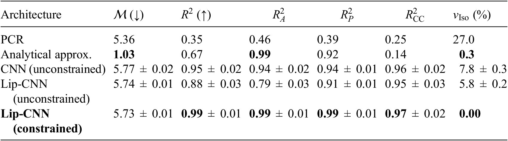
To establish performance bounds, we evaluate a linear principal component regression (PCR) baseline. PCR demonstrates poor predictive capability (overall
$ {R}^2=0.35 $
 ) and a high isoperimetric violation rate (
$ {\nu}_{\mathrm{Iso}}=27.0\% $
) and a high isoperimetric violation rate (
$ {\nu}_{\mathrm{Iso}}=27.0\% $
 ), confirming the highly nonlinear mapping from physical fields to integral-geometric measures (Table 1). Conversely, the analytical approximation achieves the lowest Minkowski image loss (
$ \mathcal{M}=1.03 $
), confirming the highly nonlinear mapping from physical fields to integral-geometric measures (Table 1). Conversely, the analytical approximation achieves the lowest Minkowski image loss (
$ \mathcal{M}=1.03 $
 ) and near-zero isoperimetric violations (0.3%). While perfectly capturing the area (
$ {R}_A^2=0.99 $
) and near-zero isoperimetric violations (0.3%). While perfectly capturing the area (
$ {R}_A^2=0.99 $
 ) and approximating perimeter well (
$ {R}_P^2=0.92 $
) and approximating perimeter well (
$ {R}_P^2=0.92 $
 ), its overall
$ {R}^2 $
), its overall
$ {R}^2 $
 (0.67) is hindered by a near-complete failure to predict connected components (
$ {R}_{\mathrm{CC}}^2=0.14 $
(0.67) is hindered by a near-complete failure to predict connected components (
$ {R}_{\mathrm{CC}}^2=0.14 $
 ; see Supplementary Appendix C).
Comparison of analytical approximation and emulation
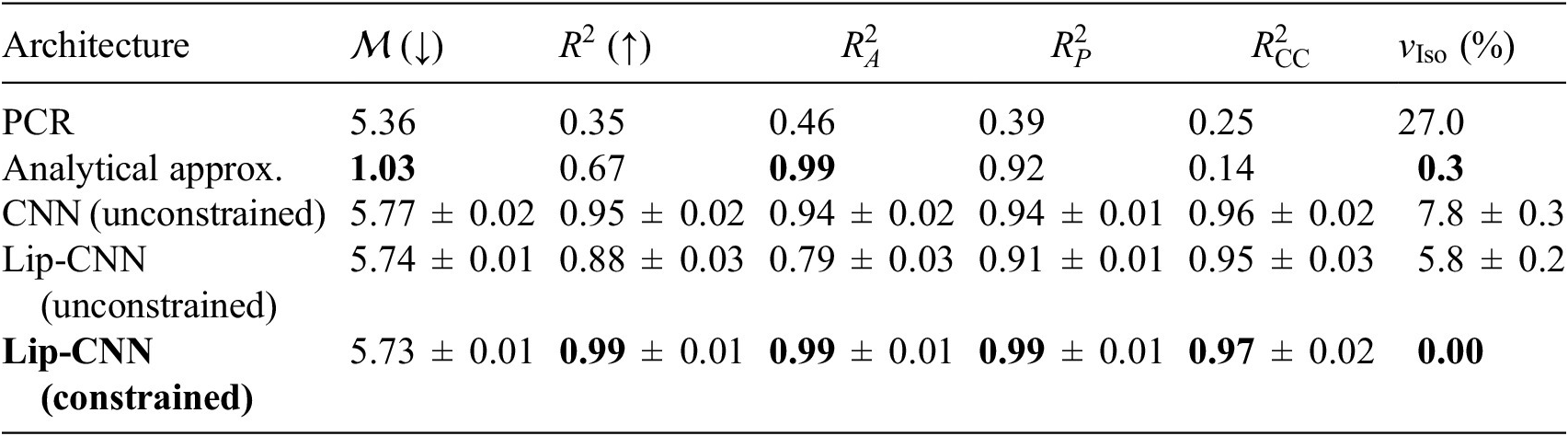
Table 1. Long description
The table consists of seven columns: Architecture, M (down arrow), R-squared (up arrow), R sub A-squared, R sub P-squared, R sub C C-squared, and nu sub Iso (%).
1. P C R: M 5.36, R-squared 0.35, R sub A-squared 0.46, R sub P-squared 0.39, R sub C C-squared 0.25, nu sub Iso 27.0.
2. Analytical approx.: M 1.03, R-squared 0.67, R sub A-squared 0.99, R sub P-squared 0.92, R sub C C-squared 0.14, nu sub Iso 0.3.
3. C N N (unconstrained): M 5.77 plus or minus 0.02, R-squared 0.95 plus or minus 0.02, R sub A-squared 0.94 plus or minus 0.02, R sub P-squared 0.94 plus or minus 0.01, R sub C C-squared 0.96 plus or minus 0.02, nu sub Iso 7.8 plus or minus 0.3.
4. Lip-C N N (unconstrained): M 5.74 plus or minus 0.01, R-squared 0.88 plus or minus 0.03, R sub A-squared 0.79 plus or minus 0.03, R sub P-squared 0.91 plus or minus 0.01, R sub C C-squared 0.95 plus or minus 0.03, nu sub Iso 5.8 plus or minus 0.2.
5. Lip-C N N (constrained): M 5.73 plus or minus 0.01, R-squared 0.99 plus or minus 0.01, R sub A-squared 0.99 plus or minus 0.01, R sub P-squared 0.99 plus or minus 0.01, R sub C C-squared 0.97 plus or minus 0.02, nu sub Iso 0.00.
Note. Bold values represent the best significant results (column wise). Performance is measured via the Minkowski image loss
$ \mathcal{M} $
 (lower is better), the coefficient of determination
$ {R}^2 $
(lower is better), the coefficient of determination
$ {R}^2 $
 for the full vector and individual components (area [A], perimeter [P], connected components [CC]), and the rate of isoperimetric violations (
$ {\nu}_{Iso} $
for the full vector and individual components (area [A], perimeter [P], connected components [CC]), and the rate of isoperimetric violations (
$ {\nu}_{Iso} $
 ).
).
While all neural architectures converged, the constrained Lip-CNN achieves the best performance across all metrics, definitively eliminating isoperimetric violations (
$ {\nu}_{\mathrm{Iso}}=0\% $
 ). The unconstrained Lip-CNN underperforms the vanilla CNN baseline; while
$ \mathcal{M} $
). The unconstrained Lip-CNN underperforms the vanilla CNN baseline; while
$ \mathcal{M} $
 remains comparable,
$ {R}^2 $
remains comparable,
$ {R}^2 $
 scores degrade significantly (e.g., area
$ 0.94\to 0.79 $
scores degrade significantly (e.g., area
$ 0.94\to 0.79 $
 ). Imposing spectral normalization bounds the Lipschitz constant, limiting representation power. Without geometric constraint heads, this “stiffened” backbone struggles to fit high-variance data. Pairing the Lipschitz backbone with geometric constraints (Lip-CNN Constr.) recovers and surpasses baseline performance. Architectural inductive biases (monotonicity and isoperimetry) effectively reduce hypothesis space complexity, acting as a scaffold that allows the stable backbone to converge to a physically valid solution despite reduced capacity. Supplementary Appendix D.1 provides further evaluation and examples of the emulators’ capabilities.
4.2. Diagnostic inversion and gradient stability
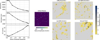
Figure 3 demonstrates that both the vanilla CNN and constrained Lip-CNN reconstruct coherent precipitation structures from geometric signatures, confirming Minkowski functionals encode sufficient morphological information to guide optimization from Gaussian noise to a localized storm object. However, textural quality diverges: the vanilla CNN produces disjointed, “blob-like” structures with sharp, artificial boundaries, whereas Lipschitz-regularized models generate continuous intensity gradients that naturally reproduce the smooth decay from convective cores to stratiform peripheries. In Supplementary Appendices D.2 and D.3, we report further evaluation of the constrained Lip-CNN emulator’s gradient quality.
Feature inversion results. Qualitative comparison of precipitation fields reconstructed by inverting the target Minkowski vector
$ {\boldsymbol{\gamma}}_{\mathrm{gt}} $
 for a test sample (left). All architectures recover the storm’s magnitude, while only constrained models generate coherent, smooth intensity gradients characteristic of convective cells (bottom left).
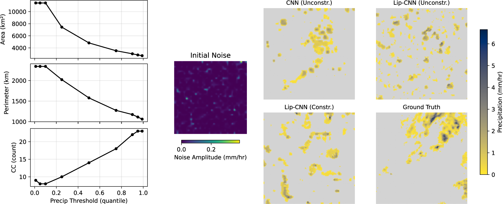
Figure 3. Long description
The visualization is divided into three main sections.
1. Left Section: Three vertically stacked line graphs share a common x-axis labeled Precip Threshold (quantile) ranging from 0.0 to 1.0.
- The top graph shows Area (km squared) decreasing from approximately 11,000 to 3,000 as the threshold increases.
- The middle graph shows Perimeter (km) decreasing from approximately 2,400 to 1,000.
- The bottom graph shows C C (count) initially dipping then increasing from 8 to 23.
2. Middle Section: A square heatmap titled Initial Noise showing a dark purple field with scattered teal and yellow specks. A horizontal color bar below it indicates Noise Amplitude (mm/hr) from 0.0 to 0.4.
3. Right Section: A two-by-two grid of precipitation maps and a vertical color bar.
- Top-Left: C N N (Unconstr.) shows fragmented yellow clusters on a gray background.
- Top-Right: Lip-C N N (Unconstr.) shows highly pixelated, noisy yellow and dark gray spots.
- Bottom-Left: Lip-C N N (Constr.) shows smoother, coherent yellow and dark blue clusters resembling storm cells.
- Bottom-Right: Ground Truth shows the target precipitation field with smooth gradients and high-intensity dark blue cores.
- Far Right: A vertical color bar for Precipitation (mm/hr) ranges from 0 (yellow) to over 6 (dark blue).
4.3. Deterministic super-resolution
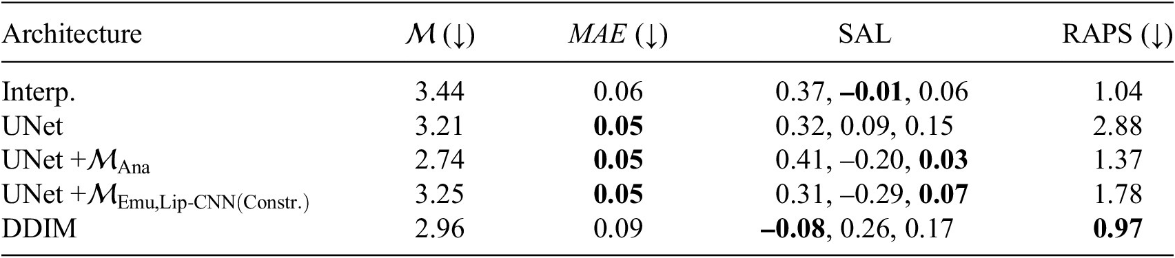
Table 2 details super-resolution performance metrics. The bicubic interpolation baseline exhibits seemingly strong spectral fidelity (RAPS = 1.04). However, this metric is an artifact of spatial smoothing; interpolation merely redistributes low-frequency kinetic energy without generating physical high-frequency features. This failure is captured by its high topological error (
$ \mathcal{M}=3.44 $
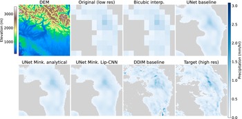
 ) and blocky visual structure (Figure 4).
Quantitative comparison of super-resolution deterministic architectures
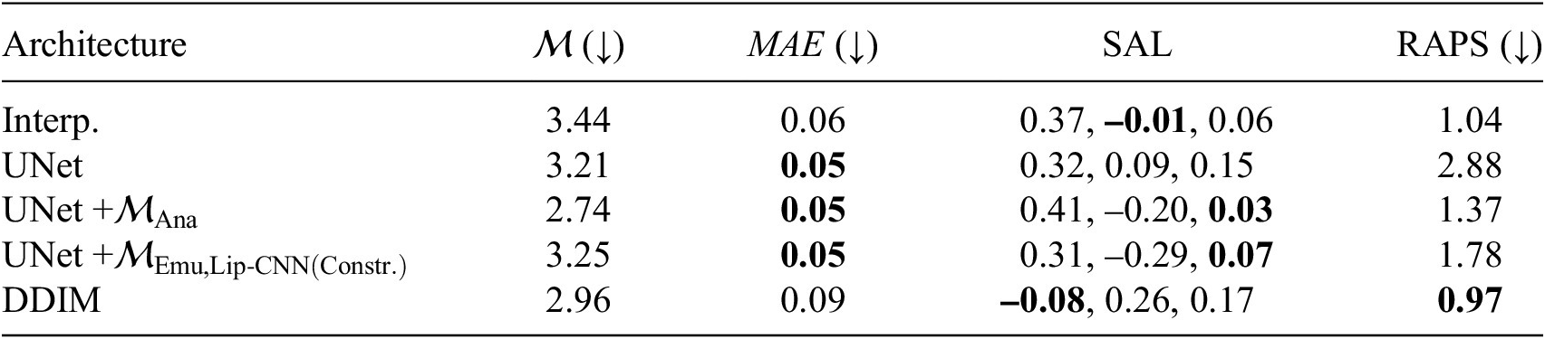
Table 2. Long description
The table consists of five columns: Architecture, M (Minkowski image loss), M A E (Mean Absolute Error), S A L (Structure-Amplitude-Location), and R A P S (Radially Averaged Power Spectral density). Downward arrows indicate that lower values are better for M, M A E, and R A P S.
* Interp.: M 3.44, M A E 0.06, S A L 0.37, -0.01, 0.06, R A P S 1.04.
* U Net: M 3.21, M A E 0.05, S A L 0.32, 0.09, 0.15, R A P S 2.88.
* U Net plus M sub Ana: M 2.74, M A E 0.05, S A L 0.41, -0.20, 0.03, R A P S 1.37.
* U Net plus M sub Emu, Lip-C N N (Constr.): M 3.25, M A E 0.05, S A L 0.31, -0.29, 0.07, R A P S 1.78.
* D D I M: M 2.96, M A E 0.09, S A L -0.08, 0.26, 0.17, R A P S 0.97.
Bolded values indicating best performance include M A E of 0.05 for all U Net variants, S A L components for Interp. (-0.01), U Net plus M sub Ana (0.03), U Net plus M sub Emu (0.07), and D D I M (-0.08), and R A P S for D D I M (0.97).
Note. Bold values represent the best significant results (column wise). Performance is measured via the Minkowski image loss (
$ \mathcal{M} $
 ), the mean absolute error (MAE), the structure-amplitude-location (SAL) metric, and the radially averaged power spectral density (RAPS) error.
Structural fidelity in precipitation downscaling. The unconstrained UNet produces an amorphous shield, missing localized convective peaks. Integral-geometric constraints (analytical and Lip-CNN) yield only marginal improvement. The stochastic DDIM baseline recovers textural realism and multiscale variance, confirming the limitations of deterministic optimization.
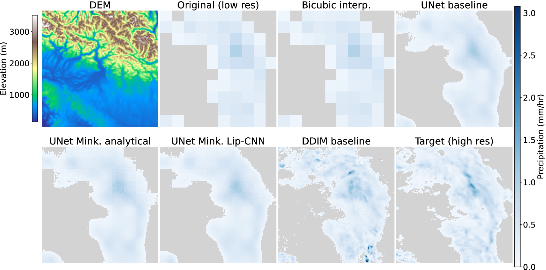
Figure 4. Long description
The figure contains two rows of four panels each.
Vertical color bars define the scales. On the far left, a scale for Elevation in meters ranges from 0 to 3000, transitioning from blue to green, yellow, and brown. On the far right, a scale for Precipitation in millimeters per hour ranges from 0.0 to 3.0, transitioning from white to dark blue.
Top Row:
1. D E M: A topographic map showing mountainous terrain in the North and West with lower elevations in the South.
2. Original low res: A coarse, pixelated grid showing light blue precipitation values.
3. Bicubic interp.: A smoothed version of the low-resolution grid with blurred edges.
4. U Net baseline: A continuous, soft-edged blue shape that lacks internal detail or peaks.
Bottom Row:
5. U Net Mink. analytical: Similar to the baseline but with slightly more defined central intensity.
6. U Net Mink. Lip-C N N: Shows a slightly more concentrated core of precipitation compared to the analytical version.
7. D D I M baseline: A highly detailed, textured map with granular blue spots that mimic the stochastic nature of real weather.
8. Target high res: The ground truth data showing sharp, localized convective peaks and complex multiscale variance. The D D I M baseline most closely resembles this panel in texture.
Comparing the baseline UNet with topologically constrained architectures illustrates deterministic optimization challenges. The unconstrained UNet minimizes spatial distortion (MAE = 0.05) but actively dampens spatial variance. Figure 4 confirms this: the UNet predicts an amorphous precipitation shield, failing to resolve localized convective cores, yielding the highest spectral error (RAPS = 2.88). Augmenting the UNet with the analytical Minkowski loss (
$ {\mathcal{M}}_{\mathrm{Ana}} $
 ) quantitatively improves RAPS (1.37) and topological error (
$ \mathcal{M}=2.74 $
) quantitatively improves RAPS (1.37) and topological error (
$ \mathcal{M}=2.74 $
 ) without compromising MAE (0.05). However, visually, both analytical and emulator-constrained (
$ {\mathcal{M}}_{\mathrm{Emu},\mathrm{Lip}-\mathrm{CNN}\left(\mathrm{Constr}.\right)} $
) without compromising MAE (0.05). However, visually, both analytical and emulator-constrained (
$ {\mathcal{M}}_{\mathrm{Emu},\mathrm{Lip}-\mathrm{CNN}\left(\mathrm{Constr}.\right)} $
 ) outputs only marginally improve upon the baseline. The fields remain artificially smooth, indicating that the current surrogate loss implementation insufficiently enforces morphological realism.
Benchmarked against the stochastic DDIM, a distinct trade-off emerges. The DDIM achieves the most realistic energy spectrum (RAPS = 0.97) and structure amplitude (
$ S=-0.08 $
 ), successfully synthesizing high-frequency speckle and intense peaks. However, it incurs higher pixel-wise error (MAE = 0.09). This elevated MAE manifests the double-penalty effect typical of stochastic downscaling: synthesized high-frequency details, while physically realistic in texture, misalign with ground-truth spatial coordinates. Although Minkowski-constrained UNets aim to bridge this gap by preserving exact spatial alignment, their inability to visually reproduce structural fidelity highlights a limitation. Future work must refine the weighting and optimization of integral-geometric constraints to match diffusion model quality without the associated computational sampling costs.
5. Discussion and conclusions
This work establishes a rigorous framework for integrating non-differentiable integral-geometric domain knowledge into gradient-based training loops via learned surrogates, and demonstrates it on the EUMETNET OPERA radar dataset. We successfully trained a Lipschitz-regularized neural emulator to accurately map physical precipitation fields to their corresponding Minkowski functionals, structurally enforcing critical inductive biases such as monotonicity and the isoperimetric inequality. While incorporating differentiable surrogates into deep learning is a rapidly evolving frontier (Rehmann et al., Reference Rehmann, Black, Bjorgaard, Angioi, Paleyes, Heim, Häfner and Lavin2025; Nguyen et al., Reference Nguyen, Chen, Dorigo, Gauger, Vischia, Nardi, Awais, Hanif, Abbas and Kapoor2026), our empirical results highlight fundamental challenges in transitioning from accurate metric emulation to effective generator optimization.
The constrained Lip-CNN achieved a 0% isoperimetric violation rate, definitively eliminating the physically impossible geometries produced by unconstrained baselines. However, our super-resolution experiments reveal a fundamental trade-off: hard Lipschitz constraints, while essential for preventing optimization collapse, over-smooth the latent representation. The backpropagated error signals consequently lack the localized precision required to steer fine-scale spatial features; the surrogate recognizes macroscopic geometry but cannot provide the sharp, pixel-level corrective gradients needed to define distinct convective boundaries. Emerging libraries for generalized automatic differentiation of discrete operations (Paulus et al., Reference Paulus, Geist, Musil, Hoffmann, Beker and Martius2026) offer complementary analytical tools, but sequential element-wise relaxations for complex topological metrics remain prone to gradient attenuation—reinforcing the case for a top-down learned surrogate once the gradient transfer bottleneck is resolved.
Ultimately, this framework addresses a ubiquitous requirement in Earth system science: the need to model fields where geometrical accuracy is encoded in coherent structures rather than independent grid points. For applications like statistical downscaling, where the spatial organization of extreme events directly dictates localized climate impacts, our findings underscore that formulating mathematically consistent loss functions is only half the solution. Future work must couple these rigorous topological constraints with stochastic generative architectures—such as denoising diffusion probabilistic models—to combine the strict integral-geometric guarantees of the Minkowski image loss with the textural synthesis capabilities required for full morphological realism.
Supplementary material
The supplementary material for this article can be found at http://doi.org/10.1017/eds.2026.10048.
Data availability statement
The OPERA radar data used in this study are openly available under the CC BY license. Data can be accessed via the EUMETNET Open Radar Data (ORD) API. Access requires IP whitelisting; requests should be directed to the OPERA support team (support.opera@eumetnet.eu). Comprehensive documentation for data discovery and retrieval is available at https://github.com/EUMETNET/openradardata-documentation. The code implementing the full pipeline, including the Minkowski functional emulator, the analytical approximation, and the super-resolution training and evaluation framework, is publicly available through Zenodo and GitHub at https://doi.org/10.5281/zenodo.20448779.
Acknowledgments
The authors would like to thank L. Räss for technical assistance. The authors would also like to acknowledge D. Nerini, D. Domeisen, V. Chavez, L. Moret, and O. Miralles for their contributions to the initial conceptualization of this work.
Author contribution
Conceptualization: F.Q., R.C. and T.B. Methodology: F.Q. and R.C. Software: F.Q. Formal analysis: F.Q. and R.C. Investigation: F.Q. Data curation: F.Q. Writing—original draft: F.Q. Writing—review and editing: F.Q. and T.B. Visualization: F.Q. Supervision: T.B. All authors approved the final submitted draft.
Funding statements
F.Q. and T.B. acknowledge support from the Swiss National Science Foundation (SNSF) under Grant No. 10001754 (“RobustSR” project).
Competing interest
The authors declare none.
Ethical statement
The research meets all ethical guidelines, including adherence to the legal requirements of the study country.
Provenance statement
This article is part of the Climate Informatics 2026 proceedings and was accepted in Environmental Data Science based on the Climate Informatics peer review process.







 Open access

