


1. Introduction
In many fluvial environments, large aggregations of freshwater mussels, called mussel beds, are found at the sediment–water interface (Morales et al. Reference Morales, Weber, Mynett and Newton2006; van de Koppel et al. Reference van de Koppel, Gascoigne, Theraulaz, Rietkerk, Mooij and Herman2008). In medium and large rivers, mussel beds often extend over tens of kilometres. Mussels have a shell made of two slightly asymmetrical valves that protrude into the water column as they are partially buried into the substrate. Mussels can slowly move and modify their level of burrowing, generally aligning themselves parallel to the mean flow to minimise drag and avoid displacement from the substrate. Mussels filter water rich in phytoplankton and zooplankton and, possibly, pollutants through their incurrent siphon and release filtered water (i.e. water with lower levels of nitrates) through their excurrent siphon. Mussels represent one of the dominant benthic species in river environments. They are identified as ecosystem engineers as they enhance bed stability, filter water, provide habitat for other species (e.g. micro-invertebrates, larvae) and are part of the food chain in the river ecosystem (Gutiérrez et al. Reference Gutiérrez, Jones, Strayer and Iribarne2003; Howard & Cufey Reference Howard and Cufey2006; Marion et al. Reference Marion2014; Lopes-Lima et al. Reference Lopes-Lima2017; Vaughn Reference Vaughn2018; Modesto et al. Reference Modesto, Tosato, Pilbala, Benistati, Fraccarollo, Termini, Manca, Moramarco, Sousa and Riccardi2023; Pilbala et al. Reference Pilbala2024). As such, preservation of freshwater mussels is an important challenge for the sustainable management of rivers (Riccardi et al. Reference Riccardi, Froufe, Lopes-Lima and Mazzoli2016; Lopes-Lima et al. Reference Lopes-Lima2017). The capacity of large populations of mussels to survive and fulfil their aforementioned ecological roles depends on the hydrodynamics of the aquatic habitat in which they live (Folkard & Gascoigne Reference Folkard and Gascoigne2009; Daraio et al. Reference Daraio, Weber, Newton and Nestler2010). This motivates the present study that tries to investigate how the flow and turbulence structure in an open channel with a smooth or a rough bed are affected by the presence of an array of partially protruding mussels.
From a fluid mechanics point of view, the protruding mussels play the role of large-scale roughness elements that increase flow resistance and near-bed turbulence. Compared with canonical three-dimensional (3-D) roughness elements such as cubes, spheres, rectangular prisms (e.g. Xie & Castro Reference Xie and Castro2006; Coceal et al. Reference Coceal, Dobre, Thomas and Belcher2007; Yang et al. Reference Yang, Sadique, Mittal and Meneveau2016; Cameron, Nikora & Stewart Reference Cameron, Nikora and Stewart2017), freshwater mussels have slender shells that act as anisotropic macro-roughness elements. These roughness elements are then placed over a rough bed mimicking a river gravel bed or over a smooth bed mimicking a sand bed with no bedforms. The active filtering through their inhalant and exhalant syphons induces local mass and momentum exchange, though the net flow exchange is equal to zero as the discharges through the two siphons of each mussel are equal. The presence of partially burrowed mussels at the bed of an open channel induces a special type of rough-bed boundary layer that was less studied compared with standard turbulent boundary layers developing over uniformly distributed (sand-grain) roughness or over arrays of bottom-mounted sparse roughness elements where the free-stream velocity outside the boundary layer is constant (see, e.g. Jiménez Reference Jiménez2004; Castro Reference Castro2007; Yang et al. Reference Yang, Sadique, Mittal and Meneveau2016). For the freshwater unionid mussels investigated in this study, the incurrent siphon faces upstream and the excurrent siphon is oriented upwards and slightly downstream. As such, the excurrent siphon jets provide a source of momentum for the flow moving over the top of the mussel specimens.
Once the incoming flow (typically fully developed open-channel turbulent flow over a smooth or a rough bed with uniformly distributed roughness) reaches the leading edge of a long mussel bed, an internal rough-bed boundary layer associated with the mussels starts developing inside the ‘ambient’ fully developed flow (Nikora et al. Reference Nikora, Green, Thrush, Hume and Goring2002). This special type of depth-limited boundary layers in which the velocity outside the mussel-induced internal boundary layer is not constant was recently investigated by Wu & Constantinescu (Reference Wu and Constantinescu2025) using eddy-resolving numerical simulations. Once the internal boundary layer induced by the mussels reaches the free surface, the flow continues to evolve for some distance. Eventually, a new fully developed flow regime is reached inside the open channel. As this happens, the influence of the flow upstream of the leading edge of the mussel bed disappears. This new fully developed flow regime takes place over a ‘rougher’ bed compared with the flow upstream of the mussel bed and can be characterised by two roughness scales, one associated with the protruding mussels and one associated with the riverbed roughness that generally can be characterised as nearly uniformly distributed with roughness elements touching each other (e.g. sand-grain roughness). Given the very large streamwise length of mussel beds compared with the average flow depth in most rivers containing freshwater mussels, this new fully developed regime is typically present over a large fraction of the mussel bed assuming the channel curvature is relatively small. Numerically, one can study the flow and turbulence structure associated with the new fully developed regime using simulations conducted with periodic boundary conditions in the streamwise direction. The main requirement is that the channel is long enough (i.e. $ L_{x} \gt 6D $
or 30–40h, where D is the flow depth and h is the height of the protruding mussels) for the dynamics of the largest coherent structures (i.e. streaks) to be independent of the size of the computational domain. This is an important advantage compared with experimental studies that would require a very long flume (
$ L_{x} \gt 6D $
or 30–40h, where D is the flow depth and h is the height of the protruding mussels) for the dynamics of the largest coherent structures (i.e. streaks) to be independent of the size of the computational domain. This is an important advantage compared with experimental studies that would require a very long flume ( $ L_{x} \gt 100D $
) to achieve a fully developed flow regime over the mussel bed (Zampiron et al. Reference Zampiron, Cameron, Stewart, Marusic and Nikora2022).
$ L_{x} \gt 100D $
) to achieve a fully developed flow regime over the mussel bed (Zampiron et al. Reference Zampiron, Cameron, Stewart, Marusic and Nikora2022).
Turbulent channel flows with a rough bed have been investigated extensively both experimentally and numerically. Idealised spherical, hemispherical or Gaussian elements have been commonly used in both numerical and laboratory studies to generate rough surfaces with uniformly distributed roughness (e.g. (Singh, Sandham & Williams Reference Singh, Sandham and Williams2007; Manes et al. Reference Manes, Pokrajac, McEwan and Nikora2009; Bomminayuni & Stoesser Reference Bomminayuni and Stoesser2011; Cameron et al. Reference Cameron, Nikora and Stewart2017; Jelly & Busse Reference Jelly and Busse2019). To account for the heterogeneity of natural beds, some studies were conducted with real gravels (Kirkgöz Reference Kirkgöz1989; Cooper et al. Reference Cooper, Aberle, Koll and Tait2013; Wang et al. Reference Wang, Ye, Wang and Yan2015) or deformed irregular bed surfaces (De Marchis & Napoli Reference De Marchis and Napoli2012; Nikora et al. Reference Nikora, Stoesser, Cameron, Stewart, Papadopoulos, Ouro, McSherry, Zampiron, Marusic and Falconer2019). Another category of relevant studies tried to characterise fully developed turbulent channel flow over regular or irregular arrays of sparse roughness elements. Most studies used roughness elements in the form of dunes or two-dimensional (2-D) ribs (e.g. Günther & Von Rohr Reference Günther and Von Rohr2003; Leonardi et al. Reference Leonardi, Orlandi, Smalley, Djenidi and Antonia2003; Ashrafian, Andersson & Manhart Reference Ashrafian, Andersson and Manhart2004; Coleman et al. Reference Coleman, Nikora, McLean and Schlicke2007; Nabi et al. Reference Nabi, de Vriend, Mosselman, Sloff and Shimizu2012; Chang & Constantinescu Reference Chang and Constantinescu2013; Shamloo & Pirzadeh Reference Shamloo and Pirzadeh2015). Some studies used arrays of cubical elements placed on a smooth bed (Xie & Castro Reference Xie and Castro2006; Coceal et al. Reference Coceal, Dobre, Thomas and Belcher2007; Leonardi & Castro Reference Leonardi and Castro2010; Lee, Sung & Krogstad Reference Lee, Sung and Krogstad2011; Florens, Eiff & Moulin Reference Florens, Eiff and Moulin2013; Yang et al. Reference Yang, Sadique, Mittal and Meneveau2016; Singh, Debnath & Mazumder Reference Singh, Debnath and Mazumder2017; Li & Li Reference Li and Li2020; Xu et al. Reference Xu, Altland, Yang and Kunz2021; Ma & Mahesh Reference Ma and Mahesh2023). In some cases, roughness elements of more complex shapes were used to mimic bed forms in loose-bed channels (e.g. Sarakinos & Busse Reference Sarakinos and Busse2024). One main feature of turbulent channel flows over distributed roughness is the formation of streaks whose size scales with the size of the roughness elements (Defina Reference Defina1996; Detert, Nikora & Jirka Reference Detert, Nikora and Jirka2010; Chang & Constantinescu Reference Chang and Constantinescu2013). However, it is still not clear if and how the main characteristics of the streaks change between cases with distributed roughness and with sparse roughness elements assuming the equivalent roughness height, $ K_{S} $
, is close in the two cases.
$ K_{S} $
, is close in the two cases.
Most previous studies of flow over mussel beds were conducted in the field or in the laboratory (Monismith et al. Reference Monismith, Koseff, Thompson, O’Riordan and Nepf1990; O’Riordan et al. Reference O’Riordan, Monismith and Koseff1993, Reference O’Riordan, Monismith and Koseff1995; Crimaldi et al. Reference Crimaldi, Thompson, Rosman, Lowe and Koseff2002; Nikora et al. Reference Nikora, Green, Thrush, Hume and Goring2002; Widdows et al. Reference Widdows, Lucas, Brinsley, Salkeld and Staff2002; van Duren et al. Reference van Duren, Herman, Sandee and Heip2006; Morales et al. Reference Morales, Weber, Mynett and Newton2006; Crimaldi, Koseff & Monismith Reference Crimaldi, Koseff and Monismith2007; Folkard & Gascoigne Reference Folkard and Gascoigne2009; Sansom et al. Reference Sansom, Bennett, Atkinson and Vaughn2020). Laboratory flume studies were performed with either live mussels (e.g. Widdows et al. Reference Widdows, Lucas, Brinsley, Salkeld and Staff2002), dead mussel bodies, artificially created surrogates (e.g. Folkard & Gascoigne Reference Folkard and Gascoigne2009) or with no protruding mussels but with pairs of protruding siphons (e.g. Crimaldi et al. Reference Crimaldi, Koseff and Monismith2007). These studies included fairly limited measurements of the flow and turbulence (e.g. vertical profiles of velocity and Reynolds stresses at a limited number of locations) and many of them ignored the mussel filtering. Accurate measurements are very difficult to perform in the immediate vicinity of the mussels, a task that gets even more complicated for high surface mussel coverage densities. In addition, in many laboratory investigations measurements were performed in a region where the flow over the mussel bed was still dependent on the flow approaching the mussel bed.
The focus of most numerical studies of flow past mussels was on investigating the flow and turbulence structure around isolated or small clusters of mussels placed on a smooth or on a rough bed and determining the drag forces acting on the protruding part of the mussel’s shell (Constantinescu, Miyawaki & Liao Reference Constantinescu, Miyawaki and Liao2013; Wu, Constantinescu & Zeng Reference Wu, Constantinescu and Zeng2020; Wu & Constantinescu Reference Wu and Constantinescu2022; Lazzarin et al. Reference Lazzarin, Constantinescu, Di Micco, Wu, Lavignani, Lo Brutto, Termini and Viero2023). Lazzarin et al. (Reference Lazzarin, Constantinescu, Wu and Viero2024) investigated the effects of the surface mussel coverage density, BC, defined as the percentage of bed surface area covered by mussels, the height of the protruding part of the mussel shell, h, and the filtering discharge on the drag forces acting on arrays of mussels partially buried in a gravel bed. Wu & Constantinescu (Reference Wu and Constantinescu2025) investigated the flow past arrays of partially burrowed mussels placed in an open channel with a smooth, horizontal bed. Their study used double averaging to investigate the effects of varying the surface mussel coverage density, the level of mussel burrowing and the filtration velocity ratio (here VR is defined as the ratio between the mean velocity of the flow inside the excurrent siphon, $ U_{\textit{ex}} $
, and the bulk channel velocity,
$ U_{\textit{ex}} $
, and the bulk channel velocity, $ U_{0} $
) on the spatial development of the 2-D turbulent boundary layer induced by the mussels. They found that, starting some distance from the leading edge of the mussel bed, the scaled double-averaged profiles of the mean streamwise velocity, turbulent kinetic energy (TKE) and concentration of the scalar entering the channel through the excurrent siphons can be considered to be self-similar inside the inertial layer (
$ U_{0} $
) on the spatial development of the 2-D turbulent boundary layer induced by the mussels. They found that, starting some distance from the leading edge of the mussel bed, the scaled double-averaged profiles of the mean streamwise velocity, turbulent kinetic energy (TKE) and concentration of the scalar entering the channel through the excurrent siphons can be considered to be self-similar inside the inertial layer ( $ h \lt z \lt \delta $
, where
$ h \lt z \lt \delta $
, where $ \delta(x) $
is the boundary layer thickness and z is the vertical direction). Following the work of Yang et al. (Reference Yang, Sadique, Mittal and Meneveau2016), an analytical model was proposed to approximate the double-averaged streamwise velocity inside the inner layer (
$ \delta(x) $
is the boundary layer thickness and z is the vertical direction). Following the work of Yang et al. (Reference Yang, Sadique, Mittal and Meneveau2016), an analytical model was proposed to approximate the double-averaged streamwise velocity inside the inner layer ( $ z \lt h $
) and inside the inertial layer where a modified log-law component was supplemented by a standard law-of-the-wake component. The scaling coefficient of the law-of-the-wake component was found to be significantly larger than typical values used to describe velocity variation in turbulent boundary layers developing in a surrounding flow with close-to-uniform free-stream velocity. No numerical study using eddy-resolving techniques had yet been conducted for fully developed open-channel flow over a mussel bed even though the flow over large parts of mussel beds in rivers is close to fully developed.
$ z \lt h $
) and inside the inertial layer where a modified log-law component was supplemented by a standard law-of-the-wake component. The scaling coefficient of the law-of-the-wake component was found to be significantly larger than typical values used to describe velocity variation in turbulent boundary layers developing in a surrounding flow with close-to-uniform free-stream velocity. No numerical study using eddy-resolving techniques had yet been conducted for fully developed open-channel flow over a mussel bed even though the flow over large parts of mussel beds in rivers is close to fully developed.
The main goal of the present paper is to describe flow and turbulence structure over an array of partially burrowed mussels placed on a smooth or a rough bed of an open channel at large distances from the leading edge of the mussel bed where the flow is fully developed. As opposed to Wu & Constantinescu (Reference Wu and Constantinescu2025), the present study is not limited to cases where the mussels can be characterised as sparse roughness elements (e.g. $ \textit{BC} \lt 0.112 $
).
$ \textit{BC} \lt 0.112 $
).
The main research questions the present study tries to answer are as follows.
-
(i) What are the main differences in terms of the mean flow and turbulence structure inside the open channel between cases with low surface mussel coverage densities and cases with densely packed mussels?
-
(ii) Does the (vertical) flow structure change significantly in cases when mussels are placed on a rough bed mimicking a gravel bed in a river compared with cases when the same mussels are placed on a smooth bed?
-
(iii) Does the three-layer analytical model proposed by Wu & Constantinescu (Reference Wu and Constantinescu2025) to describe the double-averaged velocity profile inside a boundary layer developing over a mussel bed in an open channel still apply once the flow over the mussel bed becomes fully developed? If so, are there any quantitative differences between the developing and the fully developed flow regimes?
-
(iv) How are the mussel bed characteristics (e.g. BC, VR, $ d_{50}/h $
) affecting the double-averaged profiles of the streamwise velocity, the TKE and the primary shear stress? What are the effects of the mussel bed characteristics on the equivalent bed roughness and bed friction velocity associated with the double-averaged streamwise velocity profile?
$ d_{50}/h $
) affecting the double-averaged profiles of the streamwise velocity, the TKE and the primary shear stress? What are the effects of the mussel bed characteristics on the equivalent bed roughness and bed friction velocity associated with the double-averaged streamwise velocity profile? -
(v) How does the transverse spacing of the velocity streaks generated by the mussel bed vary with the main geometrical variables characterising the mussel bed? Is the spacing of the streaks generated by the mussel bed similar to that observed for streaks forming in an open-channel flow over uniformly distributed roughness or for streaks generated over other types of large-scale roughness elements (e.g. 2-D dunes)?

2. Modelling approach and test cases
The present study used an approach that is similar to that employed by Wu & Constantinescu (Reference Wu and Constantinescu2025). This approach is based on performing detached eddy simulations (DES) in an open channel with a deformed bed surface that accounts for the protruding part of the mussels and includes the siphons through which mass exchange takes place. Similarly to Wu & Constantinescu (Reference Wu and Constantinescu2025), a realistic shape of the mussel shells is used. Identical mussels with constant h and VR are distributed randomly over the channel bed surface such that the surface mussel coverage density is close to constant in each simulation. However, the shape of the shells in the present study corresponds to a different species of mussels and, in most simulations, mussels are placed on a deformed bed surface mimicking a gravel bed with a median diameter d
50. For all cases, $ d_{50}/h \lt 0.15 $
such that there is a clear separation between the length scale associated with the gravels and that associated with the protruding mussels.
$ d_{50}/h \lt 0.15 $
such that there is a clear separation between the length scale associated with the gravels and that associated with the protruding mussels.
The present study covers the whole range of relevant surface mussel coverage densities up to the limiting case of closely packed mussels (i.e. $ \textit{BC} \gt 0.8 $
). This is important because closely packed mussels are sometimes encountered in natural environments. Moreover, such cases allow studying the transition to a skimming flow regime characterised by very little penetration of the flow from the inertial layer into the inner layer. In terms of the width- and time-averaged flow, the profiles of the mean velocity and turbulence statistics become close to independent of the streamwise direction as the simulations are performed with periodic boundary conditions in the streamwise direction. The width-averaged profiles are then averaged over the length of the computational domain such that each test case is characterised by a unique vertical profile of the (double-averaged) variable being analysed.
$ \textit{BC} \gt 0.8 $
). This is important because closely packed mussels are sometimes encountered in natural environments. Moreover, such cases allow studying the transition to a skimming flow regime characterised by very little penetration of the flow from the inertial layer into the inner layer. In terms of the width- and time-averaged flow, the profiles of the mean velocity and turbulence statistics become close to independent of the streamwise direction as the simulations are performed with periodic boundary conditions in the streamwise direction. The width-averaged profiles are then averaged over the length of the computational domain such that each test case is characterised by a unique vertical profile of the (double-averaged) variable being analysed.
2.1. Computational domain and bed topography
Simulations included in the present study were conducted in a 3-D channel with a mean flow depth D = 0.15 m (figure 1
a). The computational domain was L
x
= 1.0 m (6.66 D or 41.6 h) long and L
y
= 0.5 m (3.33 D or 20.8 h) wide. These dimensions are similar to those used in other studies of turbulent open-channel flow over a rough bed (e.g. Bomminayuni & Stoesser Reference Bomminayuni and Stoesser2011; Sarakinos & Busse Reference Sarakinos and Busse2024). In the following, x, y and z denote the streamwise, spanwise and vertical directions, respectively, while u, $ v, w $
are the corresponding velocity components. All test cases were conducted with a volumetric channel flow rate Q = 0.0123 m3s−1 that corresponded to a section-averaged, or bulk channel, velocity
$ v, w $
are the corresponding velocity components. All test cases were conducted with a volumetric channel flow rate Q = 0.0123 m3s−1 that corresponded to a section-averaged, or bulk channel, velocity $ U_{0} $
= 0.164 ms−1. The channel Froude number was 0.14 and the bulk Reynolds number was 24 600. Froude number effects are expected to remain negligible until the Froude number becomes larger than 0.5, but this regime is generally not encountered in rivers containing mussel beds.
$ U_{0} $
= 0.164 ms−1. The channel Froude number was 0.14 and the bulk Reynolds number was 24 600. Froude number effects are expected to remain negligible until the Froude number becomes larger than 0.5, but this regime is generally not encountered in rivers containing mussel beds.
Computational domain and main geometrical dimensions used in a simulation conducted with a rough bed ( $ d_{50}/h $
= 0.13) and BC = 0.280: (a) 3-D view of the mussel bed and channel; (b) detailed view from above; (c) longitudinal section AA cutting through a mussel specimen and the rough-bed surface.
$ d_{50}/h $
= 0.13) and BC = 0.280: (a) 3-D view of the mussel bed and channel; (b) detailed view from above; (c) longitudinal section AA cutting through a mussel specimen and the rough-bed surface.

The bed surface included in the model was obtained from the digitalisation of a water-worked gravel bed from a laboratory experiment conducted at the University of Palermo, Italy, using gravels with a median diameter d
50 = 3.10 mm and d
90 = 5.00 mm (Termini et al. Reference Termini, Lavignani and Benistati2022a
,
Reference Termini, Lavignani and Benistatib
). The characteristics of the gravel beds in these experiments are based on typical conditions in northern Italian rivers that contain mussel beds. The average height of the roughness elements, h
g
, was found to be very close to d
90. The d
50 and d
90 values used in the present simulations are also comparable to those used in a recent series of experiments of flow over a gravel bed containing arrays of mussels (Sansom et al. Reference Sansom, Bennett, Atkinson and Vaughn2020). The average dimensions of the mussels used in the flume experiments of Sansom et al. (Reference Sansom, Bennett, Atkinson and Vaughn2020) are close to those of the mussel specimens used in the present simulations. The conditions in the flume experiments of Sansom et al. (Reference Sansom, Bennett, Atkinson and Vaughn2020) mimic those in several rivers in the northeastern region of the US. The final model bed surface had symmetric opposite edges, which was required to be able to impose periodic boundary conditions at the lateral boundaries of the computational domain in simulations conducted with a rough bed. Some of the mussel bed simulations were conducted with a flat smooth bed (d
50 = 0.00 mm) as mussel beds can develop over a sandy substrate. Mussel beds can also develop in regions containing finer gravels (Termini et al. Reference Termini, Benistati, Pilbala, Modesto, Fraccarollo, Manca, Piccolroaz and Moramarco2025). This is why several simulations were conducted with a gravel bed with d
50 = 2.5 mm, which was obtained by reducing the vertical coordinate of the bed surface with d
50 = 3.1 mm by a factor of 2. This reduces the initial d
50 by a factor of $ \sqrt[3]{2}$
.
$ \sqrt[3]{2}$
.
In the simulations performed with a mussel bed, the shells in the array were all identical and corresponded to a reproduction of a real specimen of an Unio elongatulus mussel (Termini et al. Reference Termini, Benistati, Tosato, Pilbala, Modesto, Fraccarollo, Manca, Moramarco and Riccardi2023, Reference Termini, Benistati, Pilbala, Modesto, Fraccarollo, Manca, Piccolroaz and Moramarco2025). Unio elongatulus is a widespread native freshwater mussel in northern Italy and a representative unionid of local river systems (Modesto et al. Reference Modesto, Tosato, Pilbala, Benistati, Fraccarollo, Termini, Manca, Moramarco, Sousa and Riccardi2023). This species develops over gravel, sand and mud substrate in rivers (Marrone et al. Reference Marrone, Nardi, Cianfanelli, Govedič, Barra, Arculeo and Bodon2019). This species was chosen as part of an ongoing research effort to study eco-hydrodynamic interactions involving Mediterranean freshwater mussels, given that Unio elongatulus populations are experiencing a dramatic decline in rivers (Riccardi et al. Reference Riccardi2022). The length of the specimen’s shell was 0.08 m. The shells were oriented parallel to the incoming flow (i.e. angle of attack of 0°; see figure 1 b), which is the usual position of mussels that ensures the minimum exposure to the flow and a proper intake of nutrients (Monismith et al. Reference Monismith, Koseff, Thompson, O’Riordan and Nepf1990; Bunt, Maclsaac & Sprules Reference Bunt, Maclsaac and Sprules1993; Di Maio & Corkum Reference Di Maio and Corkum1997; Kumar et al. Reference Kumar, Kozarek, Hornbach, Hondzo and Hong2019). Though mussels in rivers are not all oriented exactly along the streamwise direction, it is customary to conduct experimental and numerical studies with all the shells aligned with the flow (e.g. Sansom et al. Reference Sansom, Bennett, Atkinson and Vaughn2020). This is because the misalignment of the individual shells is dictated by the local direction of the approaching mean flow that is controlled by the upstream shells. Consistent with the typical positioning of this species of mussels within their natural habitat, the excurrent siphon was located downstream of the incurrent siphon to minimise recirculation and maximise feeding efficiency (Di Maio & Corkum Reference Di Maio and Corkum1997; Perles, Christian & Berg Reference Perles, Christian and Berg2003), while the shells were placed with their major axis inclined at an angle of 45° with the bed, as shown in figure 1(c). Based on this arrangement, the projected length, width and height of each specimen was L = 0.055 m, b = 0.020 m and H = 0.050 m, respectively.
The level of mussel burial was the same in all simulations and corresponded to a non-dimensional mussel protrusion height $ h/H $
= 0.48 (
$ h/H $
= 0.48 ( $ h/D $
= 0.16). This level corresponds to the average exposure level for this species of mussels. In rivers, not all mussels are buried to the same level. The effect of varying the protrusion height of the individual shell with respect to an average protrusion height level was not investigated. Simulations conducted with rectangular prisms (Yang et al. Reference Yang, Sadique, Mittal and Meneveau2016) have found that the effect of randomising the height of the roughness elements with respect to a mean value is less important compared with those associated with varying BC and h.
$ h/D $
= 0.16). This level corresponds to the average exposure level for this species of mussels. In rivers, not all mussels are buried to the same level. The effect of varying the protrusion height of the individual shell with respect to an average protrusion height level was not investigated. Simulations conducted with rectangular prisms (Yang et al. Reference Yang, Sadique, Mittal and Meneveau2016) have found that the effect of randomising the height of the roughness elements with respect to a mean value is less important compared with those associated with varying BC and h.
2.2. Main variables and matrix of simulations
Surface mussel coverage density in mussel colonies depend on several factors, such as mussel species, dimensions, habitat and environmental conditions. In the present study, mussel bed densities, ρ M , between 26 mussels m−2 (BC = 0.015) and 1480 mussels m−2 (BC = 0.828) were considered (table 1). The corresponding total number of mussels, N, over the channel bed surface of area A = 0.5 m2 varied between 13 and 740. This range of ρ M covers the regimes encounters in rivers that include sparse mussel beds, moderately dense mussel beds and highly dense or fully packed mussel beds, where the shells are close to touching each other and a skimming flow regime is established with little exchange between the inertial and the inner layers (Strayer et al. Reference Strayer, Hunter, Smith and Borg1994; O’Riordan et al. Reference O’Riordan, Monismith and Koseff1995; Coco et al. Reference Coco, Thrush, Green and Hewitt2006; Sansom et al. Reference Sansom, Bennett, Atkinson and Vaughn2020).
Matrix of simulated cases and estimated values of the main parameters in the analytical model used to predict the vertical profile of the double-averaged streamwise velocity: V
M
is the volume occupied by the protruding parts of the mussels, V
I
is the total volume within the inertial layer (i.e. $ z \lt h $
), δ
m
is the height of the linear sublayer, U
m
is the velocity at the top of the linear sublayer, a is the attenuation parameter of the exponential decay assumed inside the exponential sublayer, U
h
is the velocity at the top of the inner layer, Π is the parameter of the wake function, u
τ
is the friction velocity, U
D
is the velocity at z = D,
$ z \lt h $
), δ
m
is the height of the linear sublayer, U
m
is the velocity at the top of the linear sublayer, a is the attenuation parameter of the exponential decay assumed inside the exponential sublayer, U
h
is the velocity at the top of the inner layer, Π is the parameter of the wake function, u
τ
is the friction velocity, U
D
is the velocity at z = D, $ \textit{Re}_{\tau} = u_{\tau}D/ \nu $
, d
0 is the displacement height,
$ \textit{Re}_{\tau} = u_{\tau}D/ \nu $
, d
0 is the displacement height, $ K_{S} $
is the equivalent roughness,
$ K_{S} $
is the equivalent roughness, $ K_{S}^{+} $
=
$ K_{S}^{+} $
= $ K_{S} u_{\tau}/\nu $
. An asterisk next to the value of BC denotes a simulation conducted with a regular arrangement of the shells.
$ K_{S} u_{\tau}/\nu $
. An asterisk next to the value of BC denotes a simulation conducted with a regular arrangement of the shells.

In all but two of the test cases, the shells were placed in an irregular pattern but still ensuring a close-to-constant surface mussel coverage density at scales larger than five times the average distance between neighbouring mussels. A randomisation procedure was used to assign spatial coordinates of each mussel within the array (Lazzarin et al. Reference Lazzarin, Constantinescu, Wu and Viero2024). In the simulation conducted with BC = 0.828 and a regular staggered arrangement, the shells were close to touching each other. As shown in the result sections, where results are compared for simulations conduced with an irregular and a regular staggered arrangement for the BC = 0.056, $ d_{50}/h $
= 0.13 and VR = 0.5 case, the effect of the random displacement of the mussels on the double-averaged profiles of the mean flow and turbulence statistics variables is very small. The irregular pattern is preferred because it mimics the arrangement of the shells in natural rivers. For the same reason, most flume laboratory studies are conducted with randomised arrangements of the mussels (see, e.g. Sansom et al. Reference Sansom, Bennett, Atkinson and Vaughn2020).
$ d_{50}/h $
= 0.13 and VR = 0.5 case, the effect of the random displacement of the mussels on the double-averaged profiles of the mean flow and turbulence statistics variables is very small. The irregular pattern is preferred because it mimics the arrangement of the shells in natural rivers. For the same reason, most flume laboratory studies are conducted with randomised arrangements of the mussels (see, e.g. Sansom et al. Reference Sansom, Bennett, Atkinson and Vaughn2020).
The flow rates through the two siphons of each mussel were maintained constant in time (i.e. Q
in
= Q
ex
= constant), which replicates flow conditions considered in previous experimental investigations (Monismith et al. Reference Monismith, Koseff, Thompson, O’Riordan and Nepf1990; Nishizaki & Ackerman Reference Nishizaki and Ackerman2017; Sansom, Atkinson & Bennett Reference Sansom, Atkinson and Bennett2018). Though mussels can alternate periods with strong and weak/reduced filtering, these changes generally occur over much larger time scales than those investigated in the present study. A constant filtering discharge is considered to be the best approximation to what is generally referred to as the continuous jet regime for freshwater and marine mussels (Bunt et al. Reference Bunt, Maclsaac and Sprules1993; Riisgård et al. Reference Riisgård, Jørgensen, Lundgreen, Storti, Walther, Meyer and Larsen2011). Most of the simulations were conducted with a filtering discharge of 1.3·10−6 m3 s−1, which corresponds to an average value for mussels of similar species and sizes (Kryger & Riisgård Reference Kryger and Riisgård1988; Monismith et al. Reference Monismith, Koseff, Thompson, O’Riordan and Nepf1990; Bunt et al. Reference Bunt, Maclsaac and Sprules1993). The corresponding filtration velocity ratio was VR = $ U_{\textit{ex}}/U_{0} $
= 0.5 (figure 1). Some simulations were conducted with filtering discharges of 3.3·10−8 (negligible filtering, VR ≈ 0) and 3.1·10−6 m3 s−1 (strong filtering, VR = 1.22) based on a linear extrapolation of the data of Bunt et al. (Reference Bunt, Maclsaac and Sprules1993) for a 55 mm long mussel. Similar peak filtering discharge values were also reported by Monismith et al. (Reference Monismith, Koseff, Thompson, O’Riordan and Nepf1990), Troost et al. (Reference Troost, Stamhuis, van Duren and Wolff2009) and Nishizaki & Ackerman (Reference Nishizaki and Ackerman2017). Values of the velocity ratio higher than 1.22 are not realistic for natural streams containing this species of mussels. The main geometrical and flow parameters of the simulations are summarised in table 1.
$ U_{\textit{ex}}/U_{0} $
= 0.5 (figure 1). Some simulations were conducted with filtering discharges of 3.3·10−8 (negligible filtering, VR ≈ 0) and 3.1·10−6 m3 s−1 (strong filtering, VR = 1.22) based on a linear extrapolation of the data of Bunt et al. (Reference Bunt, Maclsaac and Sprules1993) for a 55 mm long mussel. Similar peak filtering discharge values were also reported by Monismith et al. (Reference Monismith, Koseff, Thompson, O’Riordan and Nepf1990), Troost et al. (Reference Troost, Stamhuis, van Duren and Wolff2009) and Nishizaki & Ackerman (Reference Nishizaki and Ackerman2017). Values of the velocity ratio higher than 1.22 are not realistic for natural streams containing this species of mussels. The main geometrical and flow parameters of the simulations are summarised in table 1.
Several simulations were also conducted with a gravel bed and no mussels. Besides the rough-bed surface (d
50 = 3.10 mm, d
90 = 5.00 mm) used for most of the mussel bed simulations, simulations with no mussels were also conducted with surfaces that were obtained by multiplying the deformations of the original rough-bed surface by 0.5 and 2.0 in the three directions. The roughness of the resulting rough-bed surfaces were d
90 ≈ h
g
= 2.5 mm and d
90 ≈ h
g
= 10.0 mm, respectively. This allowed investigating the effects of varying the equivalent non-dimensional roughness height of the distributed roughness surface and to compare with results obtained from simulations conducted with a mussel bed with a similar value of $ K_{S} $
+
.
$ K_{S} $
+
.
2.3. Numerical model and mesh generation
Detached eddy simulations were performed using a finite-volume viscous flow solver (STARCCM+, CD Adapco). Detached eddy simulations have been successfully used to predict turbulent flows past submerged, surface-mounted isolated obstacles and past arrays of such obstacles placed in open channels (see, e.g. Chang & Constantinescu Reference Chang and Constantinescu2013; Chang, Constantinescu & Tsai Reference Chang, Constantinescu and Tsai2020; Wu et al. Reference Wu, Constantinescu and Zeng2020; Wu & Constantinescu Reference Wu and Constantinescu2022; Koken & Constantinescu Reference Koken and Constantinescu2023; Wu & Constantinescu Reference Wu and Constantinescu2025). Detached eddy simulations are a hybrid method that reduce to large eddy simulations (LES) away from the solid boundaries and to Reynolds-averaged Navier–Stokes (RANS) near them. In the present simulations, the base RANS model was the shear stress transport (SST) k–ω model (Menter, Kuntz & Langtry Reference Menter, Kuntz and Langtry2003; Rodi, Constantinescu & Stoesser Reference Rodi, Constantinescu and Stoesser2013). Its predictive abilities were shown to be at least as good as those of the original formulation of DES based on the Spalart–Allmaras model (Chang, Constantinescu & Park Reference Chang, Constantinescu and Park2007). To avoid the use of wall functions, the first grid point in the direction normal to each solid surface was placed at about five wall units or less. The Navier–Stokes equations were integrated on unstructured, Cartesian-like grids using a segregated flow solver. The SIMPLE algorithm was used to calculate an intermediate velocity based on the estimated pressure field, which was then corrected to satisfy the continuity equation (Patankar & Spalding Reference Patankar and Spalding1972). A hybrid-bounded central differences scheme (van Leer Reference Van Leer1979) was used to discretise the convective terms in the momentum equations, while the second-order central scheme was used to discretise the diffusive and pressure gradient terms. Transport equations were solved for the turbulence variables. The second-order upwind scheme was used to discretise the convective terms in these equations. An implicit second-order discretisation in time was used for the governing equations (SIMPLEC algorithm, van Doormal and Raithby Reference Van Doormall and Raithby1984). For a complete description of the model, the reader is referred to Lazzarin et al. (Reference Lazzarin, Constantinescu, Di Micco, Wu, Lavignani, Lo Brutto, Termini and Viero2023). Directly relevant for the present study, the model has been validated using data from laboratory experiments of flow past an isolated mussel placed on a rough bed (Lazzarin et al. Reference Lazzarin, Constantinescu, Di Micco, Wu, Lavignani, Lo Brutto, Termini and Viero2023) and on a smooth bed (Wu et al. Reference Wu, Constantinescu and Zeng2020).
To generate the computational model, the surfaces of the two shelves were scanned separately (see Lazzarin et al. Reference Lazzarin, Constantinescu, Di Micco, Wu, Lavignani, Lo Brutto, Termini and Viero2023 for details). Triangular meshes of these surfaces were extracted from the point clouds and then imported in the mesh generator as stereolithography files. As the scanned model of the mussel represented the shell of a dead specimen, its surface has been enriched by two additional parts representing the excurrent and incurrent siphons (Lazzarin et al. Reference Lazzarin, Constantinescu, Di Micco, Wu, Lavignani, Lo Brutto, Termini and Viero2023). Copies of the base mussel model containing the two siphons were placed over the bed surface at the same vertical elevation.
An initial fluid block was generated with the bed surface as the lower face. Then, the 3-D volumes of the mussels were subtracted from this fluid block volume and the new fluid block volume was meshed. A nested mesh procedure was used to generate the full grid, with cell sizes decreasing from the upper part to the lower part of the water column (Lazzarin et al. Reference Lazzarin, Constantinescu, Di Micco, Wu, Lavignani, Lo Brutto, Termini and Viero2023, Reference Lazzarin, Constantinescu, Wu and Viero2024). In the region close to the mussels and the bed, the computational grid contained cells with a mean size of 0.0012 m (≈ 14 wall units) for the simulations listed in table 1. The mesh was further refined near the siphons using cells of a mean size of 0.0005 m (≈ 5 wall units). This level of mesh refinement is similar to that used in previous numerical studies of flow past isolated arrays of mussels using DES (Wu & Constantinescu Reference Wu and Constantinescu2025). Around 13 million cells were used to mesh the computational domain in the simulations discussed in the result sections. A grid sensitivity analysis was conducted to check that the level of mesh refinement around each mussel was sufficient to obtain a grid independent solution (§ 2.5, see also Lazzarin et al. Reference Lazzarin, Constantinescu, Wu and Viero2024).
Periodic boundary conditions were applied in the longitudinal and transversal directions with a prescribed value of the water discharge, as in Lazzarin et al. (Reference Lazzarin, Constantinescu, Wu and Viero2024). Froude numbers in natural streams where mussel beds develop are generally low and the heights of the protruding shells are much smaller than the local flow depth ( $ D/h \gt 4$
, deep flow regime). These are also the conditions considered in the present simulations. These conditions justify why the upper boundary, corresponding to the free surface, was treated as a slip (shear-free) surface (Wu & Constantinescu Reference Wu and Constantinescu2025). No-slip boundary conditions were imposed at the exposed bed surface and on the protruding parts of the shells. The standard relations for the SST model were used to specify the turbulence variables on the no-slip surfaces (Menter et al. Reference Menter, Kuntz and Langtry2003). A fixed mass flow has been assigned to the exit of each inhaling siphon. The same mass flow was injected into the computational domain through each exhaling siphon tube.
$ D/h \gt 4$
, deep flow regime). These are also the conditions considered in the present simulations. These conditions justify why the upper boundary, corresponding to the free surface, was treated as a slip (shear-free) surface (Wu & Constantinescu Reference Wu and Constantinescu2025). No-slip boundary conditions were imposed at the exposed bed surface and on the protruding parts of the shells. The standard relations for the SST model were used to specify the turbulence variables on the no-slip surfaces (Menter et al. Reference Menter, Kuntz and Langtry2003). A fixed mass flow has been assigned to the exit of each inhaling siphon. The same mass flow was injected into the computational domain through each exhaling siphon tube.
After the flow became statistically steady, the flow fields over the following 20 s (i.e. 3.3 flow-through time periods) were used to calculate the mean flow and turbulence statistics and to analyse the coherent structures. The convergence of the flow statistics was determined by analysing velocity time series at different points along the vertical direction and by comparing mean velocity and TKE profiles over different time windows (see Lazzarin et al. Reference Lazzarin, Constantinescu, Wu and Viero2024). Moreover, we checked that negligible differences were present between the double-averaged profiles calculated over the upstream half and the downstream half of the computational domain.
In the present simulations, the switch from the RANS mode to the LES mode generally occurred at a distance of 10–12 wall units from the solid surfaces. The peak values of the ratio between the eddy viscosity and the molecular viscosity were less than 10. This ratio is less than one in the region situated close to the excurrent siphons where the mesh is locally refined. This suggests that the present DES simulations that resolve the viscous sublayer are equivalent to an LES with a more sophisticated near-wall (RANS based) model replacing the use of standard wall functions.
2.4. Double-averaged flow variables
Once the 3-D fields of the mean velocity and turbulence variables were calculated, the double-averaging (i.e. in time and space) technique was applied (Nikora et al. Reference Nikora, McEwan, McLean, Coleman, Pokrajac and Walters2007a
,
Reference Nikora, McLean, Coleman, Pokrajac, McEwan, Campbell, Aberle, Clunie and Kollb
) to calculate the vertical profiles of these variables. This technique was successfully used for describing the flow over complex rough beds (see, e.g. Mignot, Barthelemy & Hurther Reference Mignot, Barthelemy and Hurther2009). Given that the flow is close to homogeneous in the streamwise direction, the time-averaged variables were averaged in both the longitudinal and spanwise directions. For example, the equations used to calculate the intrinsic double-averaged mean velocity, $ \langle \overline{u} \rangle$
, the turbulence kinetic energy,
$ \langle \overline{u} \rangle$
, the turbulence kinetic energy, $\langle \textit{TKE}\rangle ,$
and the primary Reynolds shear stress,
$\langle \textit{TKE}\rangle ,$
and the primary Reynolds shear stress, $\langle \overline{u^{\prime}w^{\prime}}\rangle$
, are
$\langle \overline{u^{\prime}w^{\prime}}\rangle$
, are
 \begin{align}\left\langle \overline{u}\right\rangle \left(z\right)=\frac{1}{{L}_{x}^{\prime}L_{y}'}{\int }_{0}^{L_{x}'}\left[{\int }_{0}^{L_{y}'}\overline{u}\left(x,y,z\right)\text{d}y\right]\text{d}x, \\[-28pt] \nonumber \end{align}
 \begin{align}\left\langle \textit{TKE}\right\rangle \left(z\right)=\frac{1}{{L}_{x}^{\prime}L_{y}'}{\int }_{0}^{L_{x}'}\left[{\int }_{0}^{L_{y}'}TKE\left(x,y,z\right)\text{d}y\right]\text{d}x, \\[-28pt] \nonumber \end{align}
 \begin{align}\big\langle \overline{u^{\prime}w^{\prime}}\big\rangle \left(z\right)=\frac{1}{{L}_{x}^{\prime}L_{y}'}{\int }_{0}^{L_{x}'}\left[{\int }_{0}^{L_{y}'}\overline{u^{\prime}w^{\prime}}\left(x,y,z\right)\text{d}y\right]\text{d}x, \\[-6pt] \nonumber \end{align}
where L
x
’ and L
y
’ denote the length and the width of the region occupied by the fluid inside the computational domain at a certain vertical position, respectively (i.e. L
x
’ and L
y
’ do not consider the interior part of the protruding shells or gravels), $\overline{\boldsymbol{\cdot }}$
denotes time averaging and
$\overline{\boldsymbol{\cdot }}$
denotes time averaging and $ \langle \cdot \rangle $
denotes spatial averaging in a horizontal plane.
$ \langle \cdot \rangle $
denotes spatial averaging in a horizontal plane.
2.5. Grid dependency study
A first grid dependency study was conducted for one representative test case (BC = 0.056, $ d_{50}/h $
= 0.0 and VR = 0.50) with a smooth bed. The finer mesh contained close to twice the number of elements of the standard mesh as a result of refining the mesh in all three directions. Figure 2 shows that the double-averaged streamwise velocity, TKE and primary Reynolds shear stress are very close in the simulations performed using the finer mesh and the standard mesh. In particular, the results are very close inside the critical region situated close to the top of the protruding mussels where the peak values of the turbulent stresses are recorded. These results are consistent with those of the grid dependency study conducted by Lazzarin et al. (Reference Lazzarin, Constantinescu, Wu and Viero2024).
$ d_{50}/h $
= 0.0 and VR = 0.50) with a smooth bed. The finer mesh contained close to twice the number of elements of the standard mesh as a result of refining the mesh in all three directions. Figure 2 shows that the double-averaged streamwise velocity, TKE and primary Reynolds shear stress are very close in the simulations performed using the finer mesh and the standard mesh. In particular, the results are very close inside the critical region situated close to the top of the protruding mussels where the peak values of the turbulent stresses are recorded. These results are consistent with those of the grid dependency study conducted by Lazzarin et al. (Reference Lazzarin, Constantinescu, Wu and Viero2024).
Double-averaged streamwise velocity (a), TKE (b) and primary Reynolds shear stress (c) for the two simulations conducted with BC = 0.056, $ d_{50}/h $
= 0.0 and VR = 0.50. Solid lines show results obtained using a mesh with a level of refinement corresponding to that of the simulations listed in table 1. Dashed lines refer to results obtained using a finer mesh in which the number of cells is roughly two times larger.
$ d_{50}/h $
= 0.0 and VR = 0.50. Solid lines show results obtained using a mesh with a level of refinement corresponding to that of the simulations listed in table 1. Dashed lines refer to results obtained using a finer mesh in which the number of cells is roughly two times larger.

A second grid dependency study was conducted for the BC = 0.015, $ d_{50}/h $
= 0.13 and VR = 0.50 case in which the bed is rough. The mesh was refined around the excurrent siphon and in the downstream region of (streamwise) length 3h where the excurrent jet aligns with the incoming flow. Inside this region, the cell size in the three directions varied between 0.0003 and 0.0005 m. This high resolution (i.e. 3–5 wall units based on the incoming turbulent flow) and the low Reynolds number of the excurrent jet (Re
j
= 96) ensured that the role of the turbulence model on the jets’ dynamics was minor in the finer mesh simulation in which the total number of cells was about 30 % larger compared with the standard mesh simulation. Comparison of the double-averaged profiles of the mean streamwise velocity and TKE in figure 3 confirms that the simulation conducted using the standard mesh can accurately predict the double-averaged quantities including in the region where the excurrent jets change orientation from vertical to horizontal.
$ d_{50}/h $
= 0.13 and VR = 0.50 case in which the bed is rough. The mesh was refined around the excurrent siphon and in the downstream region of (streamwise) length 3h where the excurrent jet aligns with the incoming flow. Inside this region, the cell size in the three directions varied between 0.0003 and 0.0005 m. This high resolution (i.e. 3–5 wall units based on the incoming turbulent flow) and the low Reynolds number of the excurrent jet (Re
j
= 96) ensured that the role of the turbulence model on the jets’ dynamics was minor in the finer mesh simulation in which the total number of cells was about 30 % larger compared with the standard mesh simulation. Comparison of the double-averaged profiles of the mean streamwise velocity and TKE in figure 3 confirms that the simulation conducted using the standard mesh can accurately predict the double-averaged quantities including in the region where the excurrent jets change orientation from vertical to horizontal.
Double-averaged streamwise velocity (a) and TKE (b) for the two simulations conducted with BC = 0.015, $ d_{50}/h $
= 0.13 and VR = 0.50. Solid lines show results obtained using a mesh with a level of refinement corresponding to that of the simulations listed in table 1. Dashed lines refer to results obtained using a finer mesh in which the level of mesh refinement was much larger in the region where the excurrent siphon jet interacts with the channel flow.
$ d_{50}/h $
= 0.13 and VR = 0.50. Solid lines show results obtained using a mesh with a level of refinement corresponding to that of the simulations listed in table 1. Dashed lines refer to results obtained using a finer mesh in which the level of mesh refinement was much larger in the region where the excurrent siphon jet interacts with the channel flow.

A third series of simulations was conducted in a smaller domain (0.1 m by 0.1 m in the horizontal directions, $ 0 \lt z \lt D $
) containing only one mussel with periodic conditions in the streamwise and spanwise directions corresponding to a regular non-staggered arrangement of the mussels in a case with BC = 0.056,
$ 0 \lt z \lt D $
) containing only one mussel with periodic conditions in the streamwise and spanwise directions corresponding to a regular non-staggered arrangement of the mussels in a case with BC = 0.056, $ d_{50}/h $
= 0 and VR = 0.50. Detached eddy simulations were conducted on a mesh using the same level of refinement as used in the simulations reported in table 1 and on a much finer mesh containing close to 5 times more cells. In the finer mesh simulation the cell size was decreased both close to and away from the mussel specimen. In particular, the grid size near the excurrent siphon and in the region where the jet aligns with the incoming flow was close to 0.00025 m, which corresponds to about 2.5 wall units. Additionally, one LES was conducted using the dynamic Smagorinsky model (standard level of refinement for the mesh). The effect of the turbulence model is fairly negligible, as one can see from comparing the double-averaged velocity and TKE profiles predicted by DES and LES in figure 4. This includes the critical region situated slightly above
$ d_{50}/h $
= 0 and VR = 0.50. Detached eddy simulations were conducted on a mesh using the same level of refinement as used in the simulations reported in table 1 and on a much finer mesh containing close to 5 times more cells. In the finer mesh simulation the cell size was decreased both close to and away from the mussel specimen. In particular, the grid size near the excurrent siphon and in the region where the jet aligns with the incoming flow was close to 0.00025 m, which corresponds to about 2.5 wall units. Additionally, one LES was conducted using the dynamic Smagorinsky model (standard level of refinement for the mesh). The effect of the turbulence model is fairly negligible, as one can see from comparing the double-averaged velocity and TKE profiles predicted by DES and LES in figure 4. This includes the critical region situated slightly above $ z/D $
= 0.16 where the excurrent jet realigns with the incoming flow. In particular, the
$ z/D $
= 0.16 where the excurrent jet realigns with the incoming flow. In particular, the $\langle \textit{TKE}\rangle$
values associated with the two peaks induced by the mussel specimen and by the excurrent jet, respectively, are close to identical in DES and LES. The mesh refinement study conducted for DES also shows that the double-averaged profiles are sufficiently close to conclude that solutions obtained on a mesh using the standard level of refinement can be considered to be grid independent.
$\langle \textit{TKE}\rangle$
values associated with the two peaks induced by the mussel specimen and by the excurrent jet, respectively, are close to identical in DES and LES. The mesh refinement study conducted for DES also shows that the double-averaged profiles are sufficiently close to conclude that solutions obtained on a mesh using the standard level of refinement can be considered to be grid independent.
Double-averaged streamwise velocity (a) and TKE (b) for the one-mussel simulations conducted with BC = 0.056, $ d_{50}/h $
= 0 and VR = 0.50. The solid black and dash-dotted green lines show DES and, respectively, LES results obtained using a mesh with the same level of refinement as that of the corresponding simulation listed in table 1. Dashed black lines refer to DES results obtained using a finer mesh.
$ d_{50}/h $
= 0 and VR = 0.50. The solid black and dash-dotted green lines show DES and, respectively, LES results obtained using a mesh with the same level of refinement as that of the corresponding simulation listed in table 1. Dashed black lines refer to DES results obtained using a finer mesh.

3. Results
3.1. General characteristics of the flow
Similar to the findings of Lazzarin et al. (Reference Lazzarin, Constantinescu, Di Micco, Wu, Lavignani, Lo Brutto, Termini and Viero2023) for isolated Unio elongatulus mussels placed on a smooth bed or on a gravel bed, no horseshoe vortices form near the junction line between the upstream face of the mussels and the bed in the present simulations with a mussel bed (see figure 5 in Lazzarin et al. (Reference Lazzarin, Constantinescu, Wu and Viero2024) and 2-D streamline patterns in figure 5 e–g). One should note that such vortices may be observed for other species and/or mussel orientations (see, e.g. figures 3 and 5 in Wu et al. Reference Wu, Constantinescu and Zeng2020).
For relatively high BC values (i.e. 0.112 ≤ BC ≤ 0.280), many mussels are basically situated in the wake of one or several upstream mussels (see, e.g. the region with $ 0.8 \lt x/D \lt 1.8 $
in figure 5
b). The separated shear layers forming at the interface between the inner and inertial layers do not extend until the downstream mussels, and there is lots of momentum exchange between the two layers driven by the energetic vortical eddies generated by the mussels and/or gravels (see figures 5
b, 5
e and 5
f). In the present study, this range of BC values corresponds to a regime that is associated with arrays composed of sparsely distributed roughness elements.
$ 0.8 \lt x/D \lt 1.8 $
in figure 5
b). The separated shear layers forming at the interface between the inner and inertial layers do not extend until the downstream mussels, and there is lots of momentum exchange between the two layers driven by the energetic vortical eddies generated by the mussels and/or gravels (see figures 5
b, 5
e and 5
f). In the present study, this range of BC values corresponds to a regime that is associated with arrays composed of sparsely distributed roughness elements.
Instantaneous spanwise vorticity, $ \omega_{y}H/U_{0} $
, in a vertical streamwise plane in the simulations conducted with BC = 0 and
$ \omega_{y}H/U_{0} $
, in a vertical streamwise plane in the simulations conducted with BC = 0 and $ d_{50}/h $
= 0.13 (a,d); BC = 0.280, VR = 0.5 and
$ d_{50}/h $
= 0.13 (a,d); BC = 0.280, VR = 0.5 and $ d_{50}/h $
= 0.13 (b,e,f); BC = 0.828, VR = 0.5 and
$ d_{50}/h $
= 0.13 (b,e,f); BC = 0.828, VR = 0.5 and $ d_{50}/h $
= 0.00 (c,g). Also shown in frames (d–g) are 2-D streamline patterns. The blue arrows point toward the (vertical) separated shear layers generated at the top of the mussels. The dark red arrows point toward energetic vortical eddies generated over the downstream parts the separated shear layers. The dashed line shows the maximum vertical extent of the region containing energetic eddies generated by mussels and/or gravels. The orange arrows in frames (e,f) point toward regions where horseshoe vortices may form.
$ d_{50}/h $
= 0.00 (c,g). Also shown in frames (d–g) are 2-D streamline patterns. The blue arrows point toward the (vertical) separated shear layers generated at the top of the mussels. The dark red arrows point toward energetic vortical eddies generated over the downstream parts the separated shear layers. The dashed line shows the maximum vertical extent of the region containing energetic eddies generated by mussels and/or gravels. The orange arrows in frames (e,f) point toward regions where horseshoe vortices may form.

At much higher surface mussel coverage densities (i.e. BC ≥ 0.6), a skimming flow regime is observed in which the streamwise velocities are very low over the lower parts of the protruding mussels (see discussion of figures 6
a and 7
b). For cases with densely packed mussels, the flow resistance and the equivalent roughness height associated with the mussels start decreasing with increasing BC (see $ K_{S} $
+
values in table 1 for the
$ K_{S} $
+
values in table 1 for the $d_{50}/h=0$
cases with BC = 0.28 and 0.828) as only the top part of each mussel contributes significantly to increasing the flow resistance. A skimming flow regime was also observed for various flows containing arrays of roughness elements or cavities. The transition to the skimming flow regime, which can also be considered to correspond to the transition from k-type to d-type roughness (Leonardi, Orlandi & Antonia Reference Leonardi, Orlandi and Antonia2007), was found to be a function of bed coverage (Jumars & Nowell Reference Jumars and Nowell1984), mean spacing between the roughness elements (Oke Reference Oke1988) and roughness density (Nepf Reference Nepf2012). For the mussels considered in the present study, the transition occurs in between BC = 0.28 (ρ
M
= 500 mussels m−2) and BC = 0.828 (ρ
M
= 1480 mussels m−2). Given that mussel bed densities in most rivers are between 50 and 200 mussels m−2, the regime where mussels can be considered to behave as sparse roughness elements is the most important for the present study.
$d_{50}/h=0$
cases with BC = 0.28 and 0.828) as only the top part of each mussel contributes significantly to increasing the flow resistance. A skimming flow regime was also observed for various flows containing arrays of roughness elements or cavities. The transition to the skimming flow regime, which can also be considered to correspond to the transition from k-type to d-type roughness (Leonardi, Orlandi & Antonia Reference Leonardi, Orlandi and Antonia2007), was found to be a function of bed coverage (Jumars & Nowell Reference Jumars and Nowell1984), mean spacing between the roughness elements (Oke Reference Oke1988) and roughness density (Nepf Reference Nepf2012). For the mussels considered in the present study, the transition occurs in between BC = 0.28 (ρ
M
= 500 mussels m−2) and BC = 0.828 (ρ
M
= 1480 mussels m−2). Given that mussel bed densities in most rivers are between 50 and 200 mussels m−2, the regime where mussels can be considered to behave as sparse roughness elements is the most important for the present study.
Bulk streamwise velocity (left) and TKE (right) inside the inner (blue symbols) and inertial (red symbols) layers as a function of (a) BC in the simulations conducted with $ d_{50}/h $
= 0.13 and VR = 0.5, (b)
$ d_{50}/h $
= 0.13 and VR = 0.5, (b) $ d_{50}/h $
in the simulations conducted with BC = 0.112 and VR = 0.5, (c) VR in the simulations conducted with BC = 0.112 and
$ d_{50}/h $
in the simulations conducted with BC = 0.112 and VR = 0.5, (c) VR in the simulations conducted with BC = 0.112 and $ d_{50}/h $
= 0.13.
$ d_{50}/h $
= 0.13.

In cases with sparsely distributed mussels placed on a gravel bed (figure 5
b), mussels behave qualitatively similarly to the larger gravels (figure 5
a) in terms of their capacity to generate energetic vortical eddies. For both types of roughness elements, flow separation is generally observed at their back (see, e.g. the recirculation regions in figures 5
dand 5
f), while strong separated shear layers are generated around the top of the elements (see blue arrows in figures 5
a and 5
b). The separated shear layers generated by the mussels most often are not close to horizontal and they do not reach the neighbouring downstream mussels (figure 5
b). These separated shear layers are also a main source for large-scale turbulence as the growth of the Kelvin–Helmholtz instabilities generates energetic vortical eddies. These eddies are visualised in figure 5(a) (see dark red arrows) for a simulation conducted with a rough bed and no mussels and in figure 5(b) for a simulation conducted with the same rough bed and with mussels (BC = 0.280). In particular, the region beneath the top of the mussels in figure 5(b) (i.e. the inner layer) is rich in vortical eddies. There is no real separation or qualitative change in the eddy structure occurring near the top of the mussels. This is true for cases when mussels are placed on a smooth bed (not shown) or on a rough bed (see, e.g. figure 5
b). The vertical penetration distance with respect to the bed surface of the larger-scale vortical eddies generated by the roughness elements inside the inertial layer increases with increasing $ K_{S} $
+
of the bed surface (see dashed lines in figures 5
a and 5
b). Lazzarin et al. (Reference Lazzarin, Constantinescu, Wu and Viero2024) found that the presence of active filtering has a relatively minor effect on the flow structure for cases with sparsely distributed mussels.
$ K_{S} $
+
of the bed surface (see dashed lines in figures 5
a and 5
b). Lazzarin et al. (Reference Lazzarin, Constantinescu, Wu and Viero2024) found that the presence of active filtering has a relatively minor effect on the flow structure for cases with sparsely distributed mussels.
The flow patterns change dramatically once the skimming flow regime dominates. The most important qualitative change is the development of a fairly horizontal vorticity sheet touching the top part of the mussels (see, e.g. the vorticity field in figure 5(c) for BC = 0.828), similar to what is observed over arrays of low-aspect-ratio cavities. Though the vorticity sheet is not continuous and vortical eddies can still penetrate inside the inner layer, the overall effect is a strong decrease of the momentum exchange between the inner and inertial layers. Compared with cases with sparsely distributed mussels (see, e.g. figure 5 b), relatively few energetic vortical eddies are present inside the inner layer once the skimming flow regime dominates (see, e.g. figures 5 c and 5 g). Moreover, the vertical penetration length of the eddies generated inside the downstream parts of the separated shear layers decreases once the flow transitions from the sparsely distributed mussel regime to the skimming flow regime (see dashed line in figures 5 b and 5 c).
Given the stark differences of the flow inside the inner and inertial layers illustrated in figure 5, it is relevant to understand how bulk variables describing the flow beneath and above the top of the large-scale roughness elements vary with the main geometrical (BC, $ d_{50}/h $
) and flow (VR) parameters describing the mussel bed environment. Figure 6 presents results for the non-dimensional bulk streamwise velocity and TKE inside the inner
$ d_{50}/h $
) and flow (VR) parameters describing the mussel bed environment. Figure 6 presents results for the non-dimensional bulk streamwise velocity and TKE inside the inner $(U_{inner}, \textit{TKE}_{inner})$
and inertial (U
inertial
, TKE
inertial
) layers. These variables are calculated by vertically averaging
$(U_{inner}, \textit{TKE}_{inner})$
and inertial (U
inertial
, TKE
inertial
) layers. These variables are calculated by vertically averaging $ \langle\overline{u} \rangle$
and
$ \langle\overline{u} \rangle$
and $\langle \textit{TKE}\rangle$
inside the two layers.
$\langle \textit{TKE}\rangle$
inside the two layers.
For a constant velocity ratio and $ d_{50}/h $
, an increase of the surface mussel coverage density induces an increase of the drag force acting on the flow moving through the inner layer. This explains the observed decrease of the bulk inner layer velocity with increasing BC in figure 6(a). Due to continuity, the flow inside the inertial layer increases its streamwise momentum, which is the main reason why U
inertial
is increasing with BC. These trends are in agreement with experimental observations of channel flow past arrays of mussels with comparable characteristics (Sansom et al. Reference Sansom, Bennett, Atkinson and Vaughn2020). For cases with sparsely distributed mussels, the TKE inside the inertial layer increases monotonically with BC mostly because of the increase in the number of eddies shed in the vertical separated shear layers generated by the mussels. These eddies are predominantly situated inside the bottom part of the inertial layer (see, e.g. figure 5). The variation of the bulk TKE with BC is different inside the inner layer where the main contributors are eddies generated in the horizontal shear layers of the mussels and the gravels (Lazzarin et al. Reference Lazzarin, Constantinescu, Di Micco, Wu, Lavignani, Lo Brutto, Termini and Viero2023, Reference Lazzarin, Constantinescu, Wu and Viero2024). The peak value of TKE
inner
is observed for BC = 0.112.
$ d_{50}/h $
, an increase of the surface mussel coverage density induces an increase of the drag force acting on the flow moving through the inner layer. This explains the observed decrease of the bulk inner layer velocity with increasing BC in figure 6(a). Due to continuity, the flow inside the inertial layer increases its streamwise momentum, which is the main reason why U
inertial
is increasing with BC. These trends are in agreement with experimental observations of channel flow past arrays of mussels with comparable characteristics (Sansom et al. Reference Sansom, Bennett, Atkinson and Vaughn2020). For cases with sparsely distributed mussels, the TKE inside the inertial layer increases monotonically with BC mostly because of the increase in the number of eddies shed in the vertical separated shear layers generated by the mussels. These eddies are predominantly situated inside the bottom part of the inertial layer (see, e.g. figure 5). The variation of the bulk TKE with BC is different inside the inner layer where the main contributors are eddies generated in the horizontal shear layers of the mussels and the gravels (Lazzarin et al. Reference Lazzarin, Constantinescu, Di Micco, Wu, Lavignani, Lo Brutto, Termini and Viero2023, Reference Lazzarin, Constantinescu, Wu and Viero2024). The peak value of TKE
inner
is observed for BC = 0.112.
For constant BC and VR, increasing the distributed bed roughness induces only a small decrease of the bulk velocity inside the inner layer (figure 6
b). Stronger effects are observed for the TKE, as the presence of gravels generates energetic vortical eddies (see, e.g. figure 3
b), some of them being eventually advected inside the inertial layer. This explains the monotonic increase of TKE
inner
and TKE
inertial
with $ d_{50}/h $
in figure 6(b). The effects of varying the filtering discharge for constant BC and
$ d_{50}/h $
in figure 6(b). The effects of varying the filtering discharge for constant BC and $ d_{50}/h $
on the bulk streamwise velocity and TKE in the two layers are fairly minor. The only noticeable effect is the slight increase of TKE
inertial
with the velocity ratio driven by eddies generated at the bottom of the inertial layer as the excurrent siphon jets align with the streamwise direction (see also figures 5 and 6 in Lazzarin et al. Reference Lazzarin, Constantinescu, Wu and Viero2024).
$ d_{50}/h $
on the bulk streamwise velocity and TKE in the two layers are fairly minor. The only noticeable effect is the slight increase of TKE
inertial
with the velocity ratio driven by eddies generated at the bottom of the inertial layer as the excurrent siphon jets align with the streamwise direction (see also figures 5 and 6 in Lazzarin et al. Reference Lazzarin, Constantinescu, Wu and Viero2024).
3.2. Double-averaged profiles
The effect of varying the surface mussel coverage density in the cases where the sparsely distributed mussel regime dominates is investigated by comparing simulations conducted with 0.056 ≤ BC ≤ 0.28, a rough bed ( $ d_{50}/h $
= 0.13) and an average value of the filtering discharge (VR = 0.5). The limiting case of a rough bed with no mussels (i.e. BC = 0) is also included. The effect of the change in the flow regime from sparsely distributed mussel regime to skimming flow regime is investigated by comparing results for the simulations conducted with a smooth bed, VR = 0.5 and with BC = 0.28 and BC = 0.828. The effect of the presence of a gravel bed in cases where the sparsely distributed mussel regime dominates is investigated by comparing results for the simulations conducted with VR = 0.5 with a smooth bed surface (
$ d_{50}/h $
= 0.13) and an average value of the filtering discharge (VR = 0.5). The limiting case of a rough bed with no mussels (i.e. BC = 0) is also included. The effect of the change in the flow regime from sparsely distributed mussel regime to skimming flow regime is investigated by comparing results for the simulations conducted with a smooth bed, VR = 0.5 and with BC = 0.28 and BC = 0.828. The effect of the presence of a gravel bed in cases where the sparsely distributed mussel regime dominates is investigated by comparing results for the simulations conducted with VR = 0.5 with a smooth bed surface ( $ d_{50}/h $
= 0) and with distributed bed roughness (
$ d_{50}/h $
= 0) and with distributed bed roughness ( $ d_{50}/h $
= 0.13). The comparison is made for an average (BC = 0.056) and a relatively large (BC = 0.28) level of the surface mussel coverage density. The effect of the presence of small-scale roughness is not investigated in cases where the skimming flow regime dominates because this effect is negligible given the very small velocities present over the lower part of the inner layer in this regime. The effect of the filtering discharge is investigated by comparing results of simulations conducted with BC = 0.28 and a gravel bed (
$ d_{50}/h $
= 0.13). The comparison is made for an average (BC = 0.056) and a relatively large (BC = 0.28) level of the surface mussel coverage density. The effect of the presence of small-scale roughness is not investigated in cases where the skimming flow regime dominates because this effect is negligible given the very small velocities present over the lower part of the inner layer in this regime. The effect of the filtering discharge is investigated by comparing results of simulations conducted with BC = 0.28 and a gravel bed ( $ d_{50}/h $
= 0.13) and two values of the velocity ratio (VR = 0.5 and VR = 0.22), corresponding to the average and maximum values of the filtering discharge for the mussel species considered. A case with a relatively high value of BC is chosen such that this effect is the strongest. Finally, the effect of the arrangement of the mussels over the bed surface is investigated by comparing results of two simulations conducted with BC = 0.28,
$ d_{50}/h $
= 0.13) and two values of the velocity ratio (VR = 0.5 and VR = 0.22), corresponding to the average and maximum values of the filtering discharge for the mussel species considered. A case with a relatively high value of BC is chosen such that this effect is the strongest. Finally, the effect of the arrangement of the mussels over the bed surface is investigated by comparing results of two simulations conducted with BC = 0.28, $ d_{50}/h $
= 0.13 and VR = 0.15 in which mussels are distributed randomly over the bed surface while maintaining a uniform distribution at larger scales and mussels are distributed using a regular staggered arrangement, respectively.
$ d_{50}/h $
= 0.13 and VR = 0.15 in which mussels are distributed randomly over the bed surface while maintaining a uniform distribution at larger scales and mussels are distributed using a regular staggered arrangement, respectively.
Vertical profiles of the double-averaged streamwise velocity, $\langle \overline{u}\rangle$
, as a function of (a) BC in the simulations conducted with
$\langle \overline{u}\rangle$
, as a function of (a) BC in the simulations conducted with $ d_{50}/h $
= 0.13 and VR = 0.5, (b) BC in the simulations conducted with
$ d_{50}/h $
= 0.13 and VR = 0.5, (b) BC in the simulations conducted with $ d_{50}/h $
= 0.0 and VR = 0.5, (c)
$ d_{50}/h $
= 0.0 and VR = 0.5, (c) $ d_{50}/h $
in the simulations conducted with VR = 0.5, (d) VR in the simulations conducted with
$ d_{50}/h $
in the simulations conducted with VR = 0.5, (d) VR in the simulations conducted with $ d_{50}/h $
= 0.13 and BC = 0.280, (e) random versus regular distribution of the mussels in the simulations conducted with BC = 0.056,
$ d_{50}/h $
= 0.13 and BC = 0.280, (e) random versus regular distribution of the mussels in the simulations conducted with BC = 0.056, $ d_{50}/h $
= 0.13 and VR = 0.5.
$ d_{50}/h $
= 0.13 and VR = 0.5.

3.2.1. Streamwise velocity
3.2.1.1. Effects of varying BC, d50/h, VR and the mussels’ arrangement on the bed surface
The vertical distributions of the double-averaged streamwise velocity, $\langle \overline{u}\rangle$
, are qualitatively similar in the mussel-bed simulations performed with BC ≤ 0.280 and with various values of VR and
$\langle \overline{u}\rangle$
, are qualitatively similar in the mussel-bed simulations performed with BC ≤ 0.280 and with various values of VR and $ d_{50}/h $
(figure 7). These profiles are characterised by a rapid increase of
$ d_{50}/h $
(figure 7). These profiles are characterised by a rapid increase of $\langle \overline{u}\rangle$
with the distance from the location where
$\langle \overline{u}\rangle$
with the distance from the location where $\langle \overline{u}\rangle$
= 0. The rate of increase of
$\langle \overline{u}\rangle$
= 0. The rate of increase of $\langle \overline{u}\rangle$
inside the inner layer decreases with increasing surface mussel coverage density (figure 7
a) because the mussel-induced drag force per unit area is proportional to BC. By contrast, once the skimming flow regime becomes dominant,
$\langle \overline{u}\rangle$
inside the inner layer decreases with increasing surface mussel coverage density (figure 7
a) because the mussel-induced drag force per unit area is proportional to BC. By contrast, once the skimming flow regime becomes dominant, $\langle \overline{u}\rangle$
≈ 0 over a significant fraction of the inner layer (e.g. until
$\langle \overline{u}\rangle$
≈ 0 over a significant fraction of the inner layer (e.g. until $ z/h $
≈ 0.3 for the simulation conducted with BC = 0.828 shown in figure 7
b). Above the level where
$ z/h $
≈ 0.3 for the simulation conducted with BC = 0.828 shown in figure 7
b). Above the level where $\langle \overline{u}\rangle$
≈ 0, the rate of increase of
$\langle \overline{u}\rangle$
≈ 0, the rate of increase of $\langle \overline{u}\rangle$
inside the inner layer in the BC = 0.828 simulation is comparable to that observed in the simulation performed in a channel with no mussels and
$\langle \overline{u}\rangle$
inside the inner layer in the BC = 0.828 simulation is comparable to that observed in the simulation performed in a channel with no mussels and $ d_{50}/h $
= 0.13 (figure 7
a). This suggests that the skimming flow regime becomes dominant when the packing of the mussels is so high that mussels can be considered to behave similarly to standard rough surfaces with uniformly distributed roughness. Given that the channel discharge was the same in all simulations, a decrease of
$ d_{50}/h $
= 0.13 (figure 7
a). This suggests that the skimming flow regime becomes dominant when the packing of the mussels is so high that mussels can be considered to behave similarly to standard rough surfaces with uniformly distributed roughness. Given that the channel discharge was the same in all simulations, a decrease of $\langle \overline{u}\rangle$
inside the inner layer is accompanied by an increase of
$\langle \overline{u}\rangle$
inside the inner layer is accompanied by an increase of $\langle \overline{u}\rangle$
inside the top part of the inertial layer. For cases with sparsely distributed mussels, the level where the flow inside the inertial layer starts accelerating due to increasing BC is situated at z ≈ 2h.
$\langle \overline{u}\rangle$
inside the top part of the inertial layer. For cases with sparsely distributed mussels, the level where the flow inside the inertial layer starts accelerating due to increasing BC is situated at z ≈ 2h.
The presence of distributed bed roughness increases the drag acting on the bottom fluid inside the inner layer, which, in turn, decreases the rate of increase of $\langle \overline{u}\rangle$
inside the inner layer (figure 7). As BC increases and the transition to the skimming flow regime starts, this effect weakens as most of the gravels are situated inside a region containing slowly moving fluid. For example, the effect of replacing the smooth channel bed by a gravel surface with
$\langle \overline{u}\rangle$
inside the inner layer (figure 7). As BC increases and the transition to the skimming flow regime starts, this effect weakens as most of the gravels are situated inside a region containing slowly moving fluid. For example, the effect of replacing the smooth channel bed by a gravel surface with $ d_{50}/h $
= 0.13 becomes negligible in the BC = 0.280 simulations (figure 7
c).
$ d_{50}/h $
= 0.13 becomes negligible in the BC = 0.280 simulations (figure 7
c).
The effect of the active filtering on the vertical profile of $\langle \overline{u}\rangle$
is relatively minor as exemplified in figure 7(d), which compares the BC = 0.280,
$\langle \overline{u}\rangle$
is relatively minor as exemplified in figure 7(d), which compares the BC = 0.280, $ d_{50}/h $
= 0.13 simulations conduced with VR = 0.5 and VR = 1.22. In the presence of strong filtering, the vertical jets redistribute the streamwise momentum in the region situated at the bottom of the inertial layer, where these jets reorient themselves to become parallel to the streamwise direction. The end effect is a less smooth increase of
$ d_{50}/h $
= 0.13 simulations conduced with VR = 0.5 and VR = 1.22. In the presence of strong filtering, the vertical jets redistribute the streamwise momentum in the region situated at the bottom of the inertial layer, where these jets reorient themselves to become parallel to the streamwise direction. The end effect is a less smooth increase of $\langle \overline{u}\rangle$
with z compared with cases with small, or no, mussel filtering.
$\langle \overline{u}\rangle$
with z compared with cases with small, or no, mussel filtering.
Finally, the random mussel distribution on the channel bed has a negligible effect on the double-averaged streamwise velocity profiles as illustrated in figure 7(e), which compares the predicted profiles from two simulations conducted with BC = 0.056, $ d_{50}/h $
= 0.13 and VR = 0.5 in which a random and, respectively, a staggered regular distribution of the mussels was used. Though significant differences are observed between the local mean vertical velocity profiles, the double-averaged profiles are quite insensitive to the way the mussels are placed on the bed, provided that the distribution of the shells can still be considered uniform at scales larger than 5 times the average distance between the shells.
$ d_{50}/h $
= 0.13 and VR = 0.5 in which a random and, respectively, a staggered regular distribution of the mussels was used. Though significant differences are observed between the local mean vertical velocity profiles, the double-averaged profiles are quite insensitive to the way the mussels are placed on the bed, provided that the distribution of the shells can still be considered uniform at scales larger than 5 times the average distance between the shells.
3.2.1.2. Analytical model describing the vertical distribution of the double-averaged streamwise velocity in fully developed open-channel flow over a mussel bed
Following Yang et al. (Reference Yang, Sadique, Mittal and Meneveau2016) and Wu & Constantinescu (Reference Wu and Constantinescu2025), an analytical model is proposed to approximate the distribution of $\langle \overline{u}\rangle$
inside the channel. The main difference with the model proposed by Wu & Constantinescu (Reference Wu and Constantinescu2025) is that the boundary layer width is replaced by the flow depth, D, in the present work that focuses on the fully developed flow regime. As shown in figure 8(a), the inner, or roughness, layer is divided into a linear sublayer and an exponential sublayer.
$\langle \overline{u}\rangle$
inside the channel. The main difference with the model proposed by Wu & Constantinescu (Reference Wu and Constantinescu2025) is that the boundary layer width is replaced by the flow depth, D, in the present work that focuses on the fully developed flow regime. As shown in figure 8(a), the inner, or roughness, layer is divided into a linear sublayer and an exponential sublayer.
Comparison between predicted vertical profile of $\langle \overline{u}\rangle$
and analytical model. (a) Sketch showing the linear and exponential sublayers of the inner layer and the inertial layer; (b) numerically predicted profiles of
$\langle \overline{u}\rangle$
and analytical model. (a) Sketch showing the linear and exponential sublayers of the inner layer and the inertial layer; (b) numerically predicted profiles of $\langle \overline{u}\rangle$
/
$\langle \overline{u}\rangle$
/ $ U_{0} $
and analytical model predictions for the BC = 0.280, VR = 0.5,
$ U_{0} $
and analytical model predictions for the BC = 0.280, VR = 0.5, $ d_{50}/h $
= 0.13 simulation; (c) velocity profiles in wall coordinates. Also shown in panels (b) and (c) are the predicted velocity profiles for a channel with uniformly distributed bed roughness (
$ d_{50}/h $
= 0.13 simulation; (c) velocity profiles in wall coordinates. Also shown in panels (b) and (c) are the predicted velocity profiles for a channel with uniformly distributed bed roughness ( $ d_{50}/h $
= 0.13) and no mussels.
$ d_{50}/h $
= 0.13) and no mussels.

In all simulations conducted with a mussel bed, the velocity increases linearly with z near the bed inside a region that is much larger than the viscous sublayer developing in cases with $ d_{50}/h $
= 0. Then, the velocity
$ d_{50}/h $
= 0. Then, the velocity $\langle \overline{u}\rangle$
transitions rapidly to an exponential variation starting at z = δ
m
, which identifies the boundary between the two sublayers. The velocity inside the linear sublayer (i.e.
$\langle \overline{u}\rangle$
transitions rapidly to an exponential variation starting at z = δ
m
, which identifies the boundary between the two sublayers. The velocity inside the linear sublayer (i.e. $ z \lt \delta_{m}$
) is approximated as
$ z \lt \delta_{m}$
) is approximated as
 \begin{align}\left\langle \overline{u}\right\rangle '=\frac{U_{m}z}{\delta _{m}},\end{align}
where U
m
is the value of $\langle \overline{u}\rangle$
at z = δ
m
and the prime symbol indicates the approximate variation assumed by the analytical model. Such a variation is consistent with model 3 of Nikora et al. (Reference Nikora, Koll, McEwan, McLean and Dittrich2004) for the interfacial sublayer that assumes that momentum transfer within the inner (roughness) layer is due to fluid motions comparable with, or even larger than, the height of the roughness elements.
$\langle \overline{u}\rangle$
at z = δ
m
and the prime symbol indicates the approximate variation assumed by the analytical model. Such a variation is consistent with model 3 of Nikora et al. (Reference Nikora, Koll, McEwan, McLean and Dittrich2004) for the interfacial sublayer that assumes that momentum transfer within the inner (roughness) layer is due to fluid motions comparable with, or even larger than, the height of the roughness elements.
Inside the exponential sublayer ( $ \delta_{m} \lt z \lt h$
), the velocity is approximated as
$ \delta_{m} \lt z \lt h$
), the velocity is approximated as
 \begin{align}\left\langle \overline{u}\right\rangle '=U_{h}{\rm e}^{{a(z-h)}/{h}},\end{align}
where U
h
is the value of $\langle \overline{u}\rangle$
at the top of the inner layer (z = h given that the protrusion height for all mussels in the array is constant) and a is the so-called attenuation parameter that is a function of the density and spatial distribution of the roughness elements (Yang et al. Reference Yang, Sadique, Mittal and Meneveau2016). An exponential variation is consistent with model 2 of Nikora et al. (Reference Nikora, Koll, McEwan, McLean and Dittrich2004) for the interfacial sublayer that assumes the mixing length within the inner (roughness) layer is constant. Such a model describes the variation of
$\langle \overline{u}\rangle$
at the top of the inner layer (z = h given that the protrusion height for all mussels in the array is constant) and a is the so-called attenuation parameter that is a function of the density and spatial distribution of the roughness elements (Yang et al. Reference Yang, Sadique, Mittal and Meneveau2016). An exponential variation is consistent with model 2 of Nikora et al. (Reference Nikora, Koll, McEwan, McLean and Dittrich2004) for the interfacial sublayer that assumes the mixing length within the inner (roughness) layer is constant. Such a model describes the variation of $\langle \overline{u}\rangle$
in deeply submerged plant canopies and, directly relevant for the present study, over the top part of the inner (roughness) layer for cases with tall roughness elements. Using different arguments, the model proposed by Cionco (Reference Cionco1965) also assumes an exponential variation of
$\langle \overline{u}\rangle$
in deeply submerged plant canopies and, directly relevant for the present study, over the top part of the inner (roughness) layer for cases with tall roughness elements. Using different arguments, the model proposed by Cionco (Reference Cionco1965) also assumes an exponential variation of $\langle \overline{u}\rangle$
inside the inner layer. The fact that, for the particular type of roughness analysed in the present study, a combination of models needs to be used to describe the variation of
$\langle \overline{u}\rangle$
inside the inner layer. The fact that, for the particular type of roughness analysed in the present study, a combination of models needs to be used to describe the variation of $\langle \overline{u}\rangle$
over the full height of the inner layer is also consistent with the findings of Nikora et al. (Reference Nikora, Koll, McEwan, McLean and Dittrich2004).
$\langle \overline{u}\rangle$
over the full height of the inner layer is also consistent with the findings of Nikora et al. (Reference Nikora, Koll, McEwan, McLean and Dittrich2004).
For fully developed flow in an open channel, we assume that the inertial layer extends from z = h to z = D, which formally means that the flow depth D replaces the thickness of the boundary layer induced by the mussels in the fully developed flow region; see also Das, Balachandar & Barron (Reference Das, Balachandar and Barron2022). In this region, the velocity profile is assumed to follow a modified log-law variation supplemented by a law-of-the-wake component (Yang et al. Reference Yang, Sadique, Mittal and Meneveau2016):
 \begin{align}\left\langle \overline{u}\right\rangle '=\frac{u_{\tau }}{\mathit{\kappa }}\left[ln\left(\frac{z-d_{0}}{z_{0}}\right)+ \Pi w\left(\frac{z}{D}\right)\right].\end{align}
Here u
τ
is the bed friction velocity, κ is the von Karman constant, d
0 is the displacement height (Jackson Reference Jackson1981), z
0 is the hydrodynamics roughness length and Π is the scaling coefficient of the wake function. Following Coles (Reference Coles1956), the wake function used was w( $ z/D = 2\text{sin}^{2}[\pi z/(2D)] $
. In the present simulations, d
0 is estimated as the distance from the bed where the resultant drag force is applied on the protruding part of each mussel (Wu & Constantinescu Reference Wu and Constantinescu2025). Basically, (3.3) modifies the origin of z in the standard logarithmic law used for rough surfaces by d
0. The values of u
τ
and z
0 are obtained by imposing
$ z/D = 2\text{sin}^{2}[\pi z/(2D)] $
. In the present simulations, d
0 is estimated as the distance from the bed where the resultant drag force is applied on the protruding part of each mussel (Wu & Constantinescu Reference Wu and Constantinescu2025). Basically, (3.3) modifies the origin of z in the standard logarithmic law used for rough surfaces by d
0. The values of u
τ
and z
0 are obtained by imposing $\langle \overline{u}\rangle '=\langle \overline{u}\rangle$
at the bottom and top of the inertial layer. The scaling coefficient is used as a tuning parameter to obtain the overall best agreement between
$\langle \overline{u}\rangle '=\langle \overline{u}\rangle$
at the bottom and top of the inertial layer. The scaling coefficient is used as a tuning parameter to obtain the overall best agreement between $\langle \overline{u}\rangle '$
and
$\langle \overline{u}\rangle '$
and $\langle \overline{u}\rangle$
.
$\langle \overline{u}\rangle$
.
Simulations performed with a mussel bed (BC = 0.280) and with no mussels (BC = 0) and distributed bed roughness ( $ d_{50}/h $
= 0.13) are used to illustrate how the presence of sparse, large roughness elements modifies the vertical profile of
$ d_{50}/h $
= 0.13) are used to illustrate how the presence of sparse, large roughness elements modifies the vertical profile of $\langle \overline{u}\rangle$
and how well the analytical model given by (3.1)–(3.3) can approximate the profile determined based on 3-D simulations. As shown in figure 8(b), the presence of the mussels and the associated reduction of
$\langle \overline{u}\rangle$
and how well the analytical model given by (3.1)–(3.3) can approximate the profile determined based on 3-D simulations. As shown in figure 8(b), the presence of the mussels and the associated reduction of $\langle \overline{u}\rangle$
inside the inner layer is accompanied by a change in the shape of the profile inside this layer. Equations (3.1) and (3.2) provide a good approximation of the predicted velocity profile inside the inner layer, while the boundary between the linear and exponential sublayers occurs around
$\langle \overline{u}\rangle$
inside the inner layer is accompanied by a change in the shape of the profile inside this layer. Equations (3.1) and (3.2) provide a good approximation of the predicted velocity profile inside the inner layer, while the boundary between the linear and exponential sublayers occurs around $ h/3$
(figure 8
b). An important observation is that the law-of-the-wall component does not provide a good approximation of the velocity profile over most of the inertial layer (e.g. large differences are observed between the predicted profile of
$ h/3$
(figure 8
b). An important observation is that the law-of-the-wall component does not provide a good approximation of the velocity profile over most of the inertial layer (e.g. large differences are observed between the predicted profile of $\langle \overline{u}\rangle$
and the law-of-the-wall component for
$\langle \overline{u}\rangle$
and the law-of-the-wall component for $ z/D \gt 0.3 $
in figure 8
b). However, when supplemented by a law-of-the-wake component with a properly fitted value of Π, the agreement between the predicted profile of
$ z/D \gt 0.3 $
in figure 8
b). However, when supplemented by a law-of-the-wake component with a properly fitted value of Π, the agreement between the predicted profile of $\langle \overline{u}\rangle$
and the analytical model given by (3.3) is very good. Another important observation is that, when plotted in wall coordinates, the double-averaged velocity profile for the simulation conducted with no mussels shows the correct behaviour, with a log-law region that is parallel to that expected for a smooth wall but with values of U
+
=
$\langle \overline{u}\rangle$
and the analytical model given by (3.3) is very good. Another important observation is that, when plotted in wall coordinates, the double-averaged velocity profile for the simulation conducted with no mussels shows the correct behaviour, with a log-law region that is parallel to that expected for a smooth wall but with values of U
+
= $\langle \overline{u}\rangle/u_{\tau}$
that are shifted downwards (i.e. ΔU
+
≈ 9.0 for
$\langle \overline{u}\rangle/u_{\tau}$
that are shifted downwards (i.e. ΔU
+
≈ 9.0 for $ z^{+} = zu_{\tau}/\nu \gt 200$
in figure 8(c), where ν is the molecular viscosity). When protruding mussels are present at the bed surface, the profile of U
+
does not display the usual log-law region mostly because of the large contribution of the law-of-the-wake component.
$ z^{+} = zu_{\tau}/\nu \gt 200$
in figure 8(c), where ν is the molecular viscosity). When protruding mussels are present at the bed surface, the profile of U
+
does not display the usual log-law region mostly because of the large contribution of the law-of-the-wake component.
3.2.1.3. Effects of varying BC, d50/h and VR on the main parameters of the analytical model describing the streamwise velocity variation, the bed friction velocity and the equivalent bed roughness height
Table 1 summarises the main parameters and variables of the analytical model used to approximate $\langle \overline{u}\rangle .$
Though both U
m
and δ
m
are generally affected by the values of BC and
$\langle \overline{u}\rangle .$
Though both U
m
and δ
m
are generally affected by the values of BC and $ d_{50}/h $
(table 1), the non-dimensional slope of the velocity gradient inside the linear sublayer,
$ d_{50}/h $
(table 1), the non-dimensional slope of the velocity gradient inside the linear sublayer, $ (U_{m}/U_{0})/(\delta_{m}/h)$
, varies in a narrow range (i.e. 0.13–0.18) for BC ≥ 0.056. As the siphons are situated at the top of the inner layer, the influence of the velocity ratio on the velocity profile inside the linear sublayer is negligible. For constant
$ (U_{m}/U_{0})/(\delta_{m}/h)$
, varies in a narrow range (i.e. 0.13–0.18) for BC ≥ 0.056. As the siphons are situated at the top of the inner layer, the influence of the velocity ratio on the velocity profile inside the linear sublayer is negligible. For constant $ d_{50}/h $
, the thickness of the linear sublayer decreases with increasing BC, which also means that the thickness of the exponential sublayer increases with BC. This result is consistent with the trend reported by Wu & Constantinescu (Reference Wu and Constantinescu2025) for developing, mussel-induced, boundary layers in an open channel, as well as with findings from several experimental studies (Nikora et al. Reference Nikora, Green, Thrush, Hume and Goring2002; Quinn & Ackerman Reference Quinn and Ackerman2014). However, in the present simulations of fully developed flow, the rate of decrease of δ
m
is very small for 0.056 ≤ BC ≤ 0.280, which is the range of interest for most natural streams containing mussels. Meanwhile, the effect of increasing the distributed bed roughness for a fixed value of BC is to increase the thickness of the linear sublayer. The increase of the thickness of the exponential sublayer with BC is explained by the fact that a larger part of the bottom of the mussels are situated in the wake generated by upstream mussels as the distance between the mussels decreases. In other words, the sheltering height increases with BC. For sufficiently high surface mussel coverage densities (i.e. for BC = 0.8), the sheltering height approaches the height of the roughness element (i.e. h) and transition to the skimming flow regime is complete.
$ d_{50}/h $
, the thickness of the linear sublayer decreases with increasing BC, which also means that the thickness of the exponential sublayer increases with BC. This result is consistent with the trend reported by Wu & Constantinescu (Reference Wu and Constantinescu2025) for developing, mussel-induced, boundary layers in an open channel, as well as with findings from several experimental studies (Nikora et al. Reference Nikora, Green, Thrush, Hume and Goring2002; Quinn & Ackerman Reference Quinn and Ackerman2014). However, in the present simulations of fully developed flow, the rate of decrease of δ
m
is very small for 0.056 ≤ BC ≤ 0.280, which is the range of interest for most natural streams containing mussels. Meanwhile, the effect of increasing the distributed bed roughness for a fixed value of BC is to increase the thickness of the linear sublayer. The increase of the thickness of the exponential sublayer with BC is explained by the fact that a larger part of the bottom of the mussels are situated in the wake generated by upstream mussels as the distance between the mussels decreases. In other words, the sheltering height increases with BC. For sufficiently high surface mussel coverage densities (i.e. for BC = 0.8), the sheltering height approaches the height of the roughness element (i.e. h) and transition to the skimming flow regime is complete.
As BC increases, the decay of $\langle \overline{u}\rangle$
inside the exponential sublayer will be larger with respect to the velocity at the top of the roughness layer, U
h
. This is the main reason for the observed increase of the attenuation parameter a with BC for constant
$\langle \overline{u}\rangle$
inside the exponential sublayer will be larger with respect to the velocity at the top of the roughness layer, U
h
. This is the main reason for the observed increase of the attenuation parameter a with BC for constant $ d_{50}/h $
and VR (see figure 9(a) and table 1). The increase of a with BC for constant
$ d_{50}/h $
and VR (see figure 9(a) and table 1). The increase of a with BC for constant $ d_{50}/h $
is accompanied by a decrease of U
h
(table 1). Meanwhile, U
h
is fairly insensitive to variations in VR and
$ d_{50}/h $
is accompanied by a decrease of U
h
(table 1). Meanwhile, U
h
is fairly insensitive to variations in VR and $ d_{50}/h $
(table 1). The increase of δ
m
with
$ d_{50}/h $
(table 1). The increase of δ
m
with $ d_{50}/h $
for constant BC is the main reason for the observed monotonic increase of a with
$ d_{50}/h $
for constant BC is the main reason for the observed monotonic increase of a with $ d_{50}/h $
in figure 9(b). Not surprisingly, the effect of the velocity ratio, VR, is negligible on the flow inside the exponential sublayer (figure 9
c). It is also relevant to mention that Yang et al. (Reference Yang, Sadique, Mittal and Meneveau2016) predicted a minimum value a = 0.4 for a boundary layer over cubic roughness elements for cases with negligible sheltering. The minimum value in the simulation with the lowest value of the surface mussel coverage density (i.e. BC = 0.015) is 0.5 (table 1). In the case of a mussel-induced boundary layer developing in an open channel, Wu & Constantinescu (Reference Wu and Constantinescu2025) estimated significantly lower values of a for comparable BC. This is likely due to the lower values of
$ d_{50}/h $
in figure 9(b). Not surprisingly, the effect of the velocity ratio, VR, is negligible on the flow inside the exponential sublayer (figure 9
c). It is also relevant to mention that Yang et al. (Reference Yang, Sadique, Mittal and Meneveau2016) predicted a minimum value a = 0.4 for a boundary layer over cubic roughness elements for cases with negligible sheltering. The minimum value in the simulation with the lowest value of the surface mussel coverage density (i.e. BC = 0.015) is 0.5 (table 1). In the case of a mussel-induced boundary layer developing in an open channel, Wu & Constantinescu (Reference Wu and Constantinescu2025) estimated significantly lower values of a for comparable BC. This is likely due to the lower values of $ U_{h}/U_{0}$
predicted for cases when such boundary layers develop in a depth-limited flow where the flow outside the boundary layer accelerates in the streamwise direction.
$ U_{h}/U_{0}$
predicted for cases when such boundary layers develop in a depth-limited flow where the flow outside the boundary layer accelerates in the streamwise direction.
Attenuation factor a (left) and equivalent (sand-grain) roughness height in wall units $ K_{S} $
+
(right) as a function of (a) BC in the simulations conducted with
$ K_{S} $
+
(right) as a function of (a) BC in the simulations conducted with $ d_{50}/h $
= 0.13 and VR = 0.5, (b)
$ d_{50}/h $
= 0.13 and VR = 0.5, (b) $ d_{50}/h $
in the simulations conducted with BC = 0.112 and VR = 0.5, (c) VR in the simulations conducted with BC = 0.112 and
$ d_{50}/h $
in the simulations conducted with BC = 0.112 and VR = 0.5, (c) VR in the simulations conducted with BC = 0.112 and $ d_{50}/h $
= 0.13.
$ d_{50}/h $
= 0.13.

The values of the wake parameter in the present simulations conducted with constant h are mainly a function of BC (table 1). Until the transition to the skimming flow regime starts, Π is increasing monotonically with BC, as the increase in the surface mussel coverage density accelerates the flow near the top (free surface) boundary and decelerates the flow near the bottom of the inertial layer (figure 7 a). Though this finding is consistent with the trend observed for a developing mussel-induced boundary layer in an open channel, the values of Π are much smaller in the case of fully developed flow (i.e. 0.15 ≤ Π ≤ 0.3) compared with those (0.55 ≤ Π ≤ 1.25) reported by Wu & Constantinescu (Reference Wu and Constantinescu2025) for arrays with a similar level of mussel burrowing. The large decrease of Π between developing and fully developed open-channel flows (e.g. from 1.25 to 0.2 for BC = 0.056) is mainly because in a developing boundary layer in a channel the flow at the edge of the boundary layer is driven by the accelerating flow in the ‘free-stream’ region, which induces a large wake component. This effect is not present in the case of a fully developed flow, which also explains why the range of Π values in the present simulation is close to typical values (Π ≈ 0.2) for boundary layers over large-scale roughness elements where the free-stream velocity is close to constant (Yang et al. Reference Yang, Sadique, Mittal and Meneveau2016) and in turbulent open-channel flows (e.g. Nezu & Rodi Reference Nezu and Rodi1986; Kirkgöz Reference Kirkgöz1989). Once the flow over the mussel bed transitions to the skimming flow regime, Π decreases as the mussel bed starts behaving more like uniformly distributed roughness.
The double averaging formally removes the mussels and, if present, the distributed roughness from the computational domain. However, the bed friction velocity, u
τ
, calculated based on the double-averaged velocity profile, $\langle \overline{u}\rangle$
(z), accounts for the presence of these two types of roughness. As expected, for constant surface mussel coverage density,
$\langle \overline{u}\rangle$
(z), accounts for the presence of these two types of roughness. As expected, for constant surface mussel coverage density, $ u_{\tau}/U_{0}$
, increases with
$ u_{\tau}/U_{0}$
, increases with $ d_{50}/h $
and is not affected by the velocity ratio, VR. Until the skimming flow regime is reached,
$ d_{50}/h $
and is not affected by the velocity ratio, VR. Until the skimming flow regime is reached, $ u_{\tau}/U_{0} $
increases slightly with BC (table 1), as the growth in the number of large-scale roughness elements per unit area translates into an increase of the equivalent bed roughness, as will be discussed later. For all mussel bed simulations, the ratio
$ u_{\tau}/U_{0} $
increases slightly with BC (table 1), as the growth in the number of large-scale roughness elements per unit area translates into an increase of the equivalent bed roughness, as will be discussed later. For all mussel bed simulations, the ratio $ u_{\tau}/U_{D}$
varies little with both BC and
$ u_{\tau}/U_{D}$
varies little with both BC and $ d_{50}/h $
(table 1).
$ d_{50}/h $
(table 1).
Non-dimensional vertical profiles of $\langle \overline{u}\rangle$
inside the inertial layer in wall coordinates (log-linear scale) used to estimate the values of the equivalent (sand-grain) roughness height,
$\langle \overline{u}\rangle$
inside the inertial layer in wall coordinates (log-linear scale) used to estimate the values of the equivalent (sand-grain) roughness height, $ K_{S} $
, of the log-law component of
$ K_{S} $
, of the log-law component of $\langle \overline{u}\rangle$
for z > > d
0. (a) Effect of varying BC in the simulations performed with
$\langle \overline{u}\rangle$
for z > > d
0. (a) Effect of varying BC in the simulations performed with $ d_{50}/h $
= 0.13 and VR = 0.5; (b) effect of varying
$ d_{50}/h $
= 0.13 and VR = 0.5; (b) effect of varying $ d_{50}/h $
in the VR = 0.5 simulations performed with BC = 0.056 and BC = 0.280. The dashed–dotted lines show the standard law of the wall in a fully developed open-channel flow over a rough bed with sand-grain roughness
$ d_{50}/h $
in the VR = 0.5 simulations performed with BC = 0.056 and BC = 0.280. The dashed–dotted lines show the standard law of the wall in a fully developed open-channel flow over a rough bed with sand-grain roughness $ K_{S} $
.
$ K_{S} $
.

Following Wu & Constantinescu (Reference Wu and Constantinescu2025), the profiles of $\langle \overline{u}\rangle$
are used to determine the equivalent (sand-grain) roughness height,
$\langle \overline{u}\rangle$
are used to determine the equivalent (sand-grain) roughness height, $ K_{S} $
. In the absence of the law-of-the-wake component and assuming the logarithmic layer is situated sufficiently far from the channel bed, i.e. z > > d
0, (3.3) reduces to the standard form of the law of the wall for a rough surface, i.e.
$ K_{S} $
. In the absence of the law-of-the-wake component and assuming the logarithmic layer is situated sufficiently far from the channel bed, i.e. z > > d
0, (3.3) reduces to the standard form of the law of the wall for a rough surface, i.e.
 \begin{align}\left\langle \overline{u}\right\rangle =u_{\tau }\left[\frac{1}{\mathit{\kappa }}ln\left(\frac{z}{K_{S}}\right)+B_{S}\right],\end{align}
where B
S
is the law-of-the-wall constant. Figure 10 includes the law of the wall and the associated value of $ K_{S} $
+
=
$ K_{S} $
+
= $ K_{S} $ $ u_{\tau}/U_{0}$
for fully developed flow over a rough bed with uniformly sized, sand-grain roughness. For the rough-bed surface with
$ u_{\tau}/U_{0}$
for fully developed flow over a rough bed with uniformly sized, sand-grain roughness. For the rough-bed surface with $ d_{50}/h $
= 0.13, the inferred value of
$ d_{50}/h $
= 0.13, the inferred value of $ K_{S} $
+
is 176. This corresponds to
$ K_{S} $
+
is 176. This corresponds to $ K_{S}/d_{90} $
= 2.6, which is close to standard values of this ratio assumed in rivers (i.e.
$ K_{S}/d_{90} $
= 2.6, which is close to standard values of this ratio assumed in rivers (i.e. $ K_{S}/d_{90} $
= 2.0–3.0). As expected, increasing the roughness of the bed on which the mussels are placed results in an increase of
$ K_{S}/d_{90} $
= 2.0–3.0). As expected, increasing the roughness of the bed on which the mussels are placed results in an increase of $ K_{S} $
. Results in figures 9(b) and 10(b) show that this effect decreases at high surface mussel coverage densities (e.g. the increase of
$ K_{S} $
. Results in figures 9(b) and 10(b) show that this effect decreases at high surface mussel coverage densities (e.g. the increase of $ K_{S} $
+
is of the order of 400 % for BC = 0.056 but only of about 40 % for BC = 0.280 if one compares simulations conducted with a smooth bed surface and with
$ K_{S} $
+
is of the order of 400 % for BC = 0.056 but only of about 40 % for BC = 0.280 if one compares simulations conducted with a smooth bed surface and with $ d_{50}/h $
= 0.13). This effect is expected to be negligible once the skimming flow regime is observed as the flow inside the inertial layer is not anymore affected by the smaller-scale distributed bed roughness. For comparable conditions,
$ d_{50}/h $
= 0.13). This effect is expected to be negligible once the skimming flow regime is observed as the flow inside the inertial layer is not anymore affected by the smaller-scale distributed bed roughness. For comparable conditions, $ K_{S} $
+
has similar values for fully developed channel flow and for a developing boundary layer in a channel. A direct comparison between present results and the cases investigated by Wu & Constantinescu (Reference Wu and Constantinescu2025) can be made only for a mussel bed with BC = 0.056,
$ K_{S} $
+
has similar values for fully developed channel flow and for a developing boundary layer in a channel. A direct comparison between present results and the cases investigated by Wu & Constantinescu (Reference Wu and Constantinescu2025) can be made only for a mussel bed with BC = 0.056, $ h/H $
≈ 0.5 and
$ h/H $
≈ 0.5 and $ d_{50}/h $
= 0 for which
$ d_{50}/h $
= 0 for which $ K_{S} $
+
= 76 for fully developed flow and
$ K_{S} $
+
= 76 for fully developed flow and $ K_{S} $
+
= 60 for a developing boundary layer. These values correspond to
$ K_{S} $
+
= 60 for a developing boundary layer. These values correspond to $ K_{S}/h $
≈ 1. If mussels are placed on a rough-bed surface,
$ K_{S}/h $
≈ 1. If mussels are placed on a rough-bed surface, $ K_{S}/d_{90} $
increases with respect to the limiting case where no mussels are present due to the additional ‘roughness’ provided by the mussels. For example, for
$ K_{S}/d_{90} $
increases with respect to the limiting case where no mussels are present due to the additional ‘roughness’ provided by the mussels. For example, for $ d_{50}/h $
= 0.13, the predicted
$ d_{50}/h $
= 0.13, the predicted $ K_{S}/d_{90} $
ranges between 5 and 8 for 0.056 ≤ BC ≤ 0.280 (table 1), which is about 2 times the value (
$ K_{S}/d_{90} $
ranges between 5 and 8 for 0.056 ≤ BC ≤ 0.280 (table 1), which is about 2 times the value ( $ K_{S}/d_{90} $
≈ 3) predicted in the corresponding simulation with no mussels.
$ K_{S}/d_{90} $
≈ 3) predicted in the corresponding simulation with no mussels.
For constant BC and $ d_{50}/h $
,
$ d_{50}/h $
, $ K_{S} $
+
decreases with increasing velocity ratio (figure 9(c) and table 1), though the decrease is only of the order of 10 % for 0 ≤ VR ≤ 1.22 (table 1). This effect is basically controlled by the vertical momentum of the excurrent siphon jets.
$ K_{S} $
+
decreases with increasing velocity ratio (figure 9(c) and table 1), though the decrease is only of the order of 10 % for 0 ≤ VR ≤ 1.22 (table 1). This effect is basically controlled by the vertical momentum of the excurrent siphon jets.
For constant $ d_{50}/h $
and VR,
$ d_{50}/h $
and VR, $ K_{S} $
+
increases with BC until the skimming flow regime is reached (see table 1 and figure 10
a), a result similar to that observed for developing boundary layers in open channels with a mussel bed (Wu & Constantinescu Reference Wu and Constantinescu2025). This is mainly due to the increase of the average drag force per streamwise length acting on the fluid inside the inner layer. As the flow transitions to the skimming flow regime,
$ K_{S} $
+
increases with BC until the skimming flow regime is reached (see table 1 and figure 10
a), a result similar to that observed for developing boundary layers in open channels with a mussel bed (Wu & Constantinescu Reference Wu and Constantinescu2025). This is mainly due to the increase of the average drag force per streamwise length acting on the fluid inside the inner layer. As the flow transitions to the skimming flow regime, $ K_{S} $
+
peaks before starting to decrease with increasing BC. This is because as mussels get closer to each other, the bottom part of the inner layer contributes negligibly to the drag force acting on the mussels, so the ‘effective height’ of the large-scale roughness elements starts decreasing with BC. Assuming a smooth bed,
$ K_{S} $
+
peaks before starting to decrease with increasing BC. This is because as mussels get closer to each other, the bottom part of the inner layer contributes negligibly to the drag force acting on the mussels, so the ‘effective height’ of the large-scale roughness elements starts decreasing with BC. Assuming a smooth bed, $ K_{S} $
+
in the BC = 0.828 simulation is expected to be comparable with the value predicted for a mussel bed with BC ≈ 0.224 and
$ K_{S} $
+
in the BC = 0.828 simulation is expected to be comparable with the value predicted for a mussel bed with BC ≈ 0.224 and $ d_{50}/h $
= 0. Another interesting question is what should be the size of the sediment (e.g. d
90) for the gravel bed to match the
$ d_{50}/h $
= 0. Another interesting question is what should be the size of the sediment (e.g. d
90) for the gravel bed to match the $ K_{S} $
for a mussel bed with a given BC and
$ K_{S} $
for a mussel bed with a given BC and $ d_{50}/h $
= 0. For example, present results show that a mussel bed with BC ≈ 0.15 containing mussels with a relative protrusion height
$ d_{50}/h $
= 0. For example, present results show that a mussel bed with BC ≈ 0.15 containing mussels with a relative protrusion height $ h/H $
= 0.48 placed on a smooth bed will have the same
$ h/H $
= 0.48 placed on a smooth bed will have the same $ K_{S} $
(≈ 2.6d
90) as a gravel bed with
$ K_{S} $
(≈ 2.6d
90) as a gravel bed with $ d_{50}/h $
= 0.13 (
$ d_{50}/h $
= 0.13 ( $ d_{90}/h$
= 0.21).
$ d_{90}/h$
= 0.21).
3.2.2. Turbulent kinetic energy
3.2.2.1. Effects of varying BC, d50/h, VR and the mussels’ arrangement on the bed surface
A general characteristic of the vertical profile of the double-averaged TKE in the simulations conducted with 0.056 ≤ BC ≤ 0.280 is the presence of two relative maxima, one inside the inner layer and one at the bottom of the inertial layer (figure 11
a). The peak inside the inner layer is likely associated with the generation of turbulent eddies inside the horizontal separated shear layers on the two sides of the protruding mussel and vortex shedding. The peak inside the inertial layer is primarily due to eddies shed inside the vertical separated shear layer near the top of the protruding mussels. By contrast, only one peak situated just above the inner layer is observed in mussel bed simulations where the skimming flow regime dominates (see, e.g. the results for BC = 0.828 in figure 11
b) or in simulations with distributed bed roughness but no mussels (see, e.g. the results for BC = 0 in figure 11
a). This is because for sufficiently high mussel clustering, vortex shedding and generation of energetic eddies inside the horizontal separated shear layers is suppressed. However, energetic eddies are still generated in the vertical separated shear layers (see, e.g. figure 5
c). The largest $\langle \textit{TKE} \rangle$
corresponds to the inner layer peak for low BC values. For BC ≥ 0.112, the maximum
$\langle \textit{TKE} \rangle$
corresponds to the inner layer peak for low BC values. For BC ≥ 0.112, the maximum $\langle \textit{TKE} \rangle$
occurs at the bottom of the inertial layer. Overall, the largest levels of amplification of
$\langle \textit{TKE} \rangle$
occurs at the bottom of the inertial layer. Overall, the largest levels of amplification of $\langle \textit{TKE} \rangle$
inside the water column are generated in the simulations with the largest values of
$\langle \textit{TKE} \rangle$
inside the water column are generated in the simulations with the largest values of $ K_{S} $
+
. Consistent with this,
$ K_{S} $
+
. Consistent with this, $\langle \textit{TKE} \rangle$
decreases once the skimming flow regime is established (figure 11
b).
$\langle \textit{TKE} \rangle$
decreases once the skimming flow regime is established (figure 11
b).
Vertical profiles of $\langle \textit{TKE} \rangle$
as a function of (a) BC in the simulations conducted with
$\langle \textit{TKE} \rangle$
as a function of (a) BC in the simulations conducted with $ d_{50}/h $
= 0.13 and VR = 0.5; (b) BC in the simulations conducted with
$ d_{50}/h $
= 0.13 and VR = 0.5; (b) BC in the simulations conducted with $ d_{50}/h $
= 0.0; (c)
$ d_{50}/h $
= 0.0; (c) $ d_{50}/h $
in the simulations conducted with VR = 0.5, BC = 0.056 and BC = 0.280; (d) VR in the simulations conducted with BC = 0.280 and
$ d_{50}/h $
in the simulations conducted with VR = 0.5, BC = 0.056 and BC = 0.280; (d) VR in the simulations conducted with BC = 0.280 and $ d_{50}/h $
= 0.13; (e) random versus irregular distribution of the mussels in the simulations conducted with BC = 0.056,
$ d_{50}/h $
= 0.13; (e) random versus irregular distribution of the mussels in the simulations conducted with BC = 0.056, $ d_{50}/h $
= 0.13 and VR = 0.5. Frame (f) compares the resolved and modelled components of the
$ d_{50}/h $
= 0.13 and VR = 0.5. Frame (f) compares the resolved and modelled components of the $\langle \textit{TKE} \rangle$
in the simulation conducted with BC = 0.056,
$\langle \textit{TKE} \rangle$
in the simulation conducted with BC = 0.056, $ d_{50}/h $
= 0.00 and VR = 0.5. The black and red arrows in the frame point toward the
$ d_{50}/h $
= 0.00 and VR = 0.5. The black and red arrows in the frame point toward the $\langle \textit{TKE} \rangle$
peaks inside the inner and inertial layers, respectively.
$\langle \textit{TKE} \rangle$
peaks inside the inner and inertial layers, respectively.

The presence of distributed bed roughness in the mussel bed simulations results in an increase of $\langle \textit{TKE} \rangle$
over the whole water column mainly due to the generation of energetic eddies by the gravels. However, this effect becomes negligible for BC ≥ 0.280 (figure 11
c). The main effect of increasing the mussel filtering discharge is an increase of
$\langle \textit{TKE} \rangle$
over the whole water column mainly due to the generation of energetic eddies by the gravels. However, this effect becomes negligible for BC ≥ 0.280 (figure 11
c). The main effect of increasing the mussel filtering discharge is an increase of $\langle \textit{TKE} \rangle$
inside the inertial layer (figure 11
d).
$\langle \textit{TKE} \rangle$
inside the inertial layer (figure 11
d).
The use of a regular staggered distribution of the mussels has a negligible effect on the vertical distribution of $\langle \textit{TKE} \rangle$
compared with the case when a randomised distribution is used (see, e.g. figure 11(e) that compares results for the BC = 0.056,
$\langle \textit{TKE} \rangle$
compared with the case when a randomised distribution is used (see, e.g. figure 11(e) that compares results for the BC = 0.056, $ d_{50}/h $
= 0.13, VR = 0.5 case). In particular, the peak
$ d_{50}/h $
= 0.13, VR = 0.5 case). In particular, the peak $\langle \textit{TKE} \rangle$
values inside the inner and inertial layers are very close.
$\langle \textit{TKE} \rangle$
values inside the inner and inertial layers are very close.
Given the use of DES, it is also relevant to check the relative contribution of the modelled part of $\langle \textit{TKE} \rangle$
. As an example, figure 11(f) compares the modelled and resolved parts of
$\langle \textit{TKE} \rangle$
. As an example, figure 11(f) compares the modelled and resolved parts of $\langle \textit{TKE} \rangle$
for the BC = 0.056,
$\langle \textit{TKE} \rangle$
for the BC = 0.056, $ d_{50}/h $
= 0, VR = 0.5 case. The modelled part is close to zero inside the inertial layer and over most of the exponential sublayer. The contribution of the modelled part is significant only very close to the bed surface, but the ratio between the peak values of the resolved and model parts is larger than 20. So, in a good approximation, the resolved part of the turbulence kinetic energy approximates the total value of
$ d_{50}/h $
= 0, VR = 0.5 case. The modelled part is close to zero inside the inertial layer and over most of the exponential sublayer. The contribution of the modelled part is significant only very close to the bed surface, but the ratio between the peak values of the resolved and model parts is larger than 20. So, in a good approximation, the resolved part of the turbulence kinetic energy approximates the total value of $\langle \textit{TKE} \rangle$
. This is why the modelled part of
$\langle \textit{TKE} \rangle$
. This is why the modelled part of $\langle \textit{TKE} \rangle$
was not plotted in figure 11(a–e).
$\langle \textit{TKE} \rangle$
was not plotted in figure 11(a–e).
3.2.2.2. Analytical model describing the vertical distribution of
$\langle \textit{TKE} \rangle$
inside the inertial layer for fully developed open-channel flow over a mussel bed

In the case of a mussel-induced developing boundary layer in a smooth bed open channel, Wu & Constantinescu (Reference Wu and Constantinescu2025) have shown that the scaled $\langle \textit{TKE} \rangle$
profiles inside the inertial layer are close to self-similar above the vertical location,
$\langle \textit{TKE} \rangle$
profiles inside the inertial layer are close to self-similar above the vertical location, $z_{\textit{TKE},\textit{max}}$
, where the maximum
$z_{\textit{TKE},\textit{max}}$
, where the maximum $\langle \textit{TKE} \rangle$
inside the inertial layer, TKE
max
, is observed. Inside most of the inertial layer, the decay of the
$\langle \textit{TKE} \rangle$
inside the inertial layer, TKE
max
, is observed. Inside most of the inertial layer, the decay of the $\langle \textit{TKE} \rangle$
was found to be close to exponential. As the top of the boundary layer was approached, the decay was better approximated by a linear function. The values of
$\langle \textit{TKE} \rangle$
was found to be close to exponential. As the top of the boundary layer was approached, the decay was better approximated by a linear function. The values of $\langle \textit{TKE} \rangle / \textit{TKE}_{\textit{max}}$
at the edge of the boundary layer were of the order of 0.02–0.04. The outer turbulent flow corresponded to the fully developed open-channel flow over a smooth bed. Present results obtained for a fully developed flow over a mussel bed also suggest an exponential decay of the
$\langle \textit{TKE} \rangle / \textit{TKE}_{\textit{max}}$
at the edge of the boundary layer were of the order of 0.02–0.04. The outer turbulent flow corresponded to the fully developed open-channel flow over a smooth bed. Present results obtained for a fully developed flow over a mussel bed also suggest an exponential decay of the $\langle \textit{TKE} \rangle$
, as exemplified by results in figure 12(a) for a simulation conducted with BC = 0.112,
$\langle \textit{TKE} \rangle$
, as exemplified by results in figure 12(a) for a simulation conducted with BC = 0.112, $ d_{50}/h $
= 0.13 and VR = 0.5. In the case of a fully developed flow the boundary layer width is replaced by the channel depth, D, and the scaling of the vertical coordinate is defined as
$ d_{50}/h $
= 0.13 and VR = 0.5. In the case of a fully developed flow the boundary layer width is replaced by the channel depth, D, and the scaling of the vertical coordinate is defined as
Scaled profiles of $\langle \textit{TKE} \rangle$
/TKE
max
inside the inertial layer (z > z
TKE
): (a) BC = 0.112,
$\langle \textit{TKE} \rangle$
/TKE
max
inside the inertial layer (z > z
TKE
): (a) BC = 0.112, $ d_{50}/h $
= 0.13, VR = 0.5; (b) BC = 0,
$ d_{50}/h $
= 0.13, VR = 0.5; (b) BC = 0, $ d_{50}/h $
= 0.13, VR = 0.5; (c) effect of varying BC for cases with
$ d_{50}/h $
= 0.13, VR = 0.5; (c) effect of varying BC for cases with $ d_{50}/h $
= 0.13 and VR = 0.5. The dashed lines show the DES predictions while the solid lines show the analytical model predictions.
$ d_{50}/h $
= 0.13 and VR = 0.5. The dashed lines show the DES predictions while the solid lines show the analytical model predictions.

 \begin{align}{z}_{\textit{TKE}}^{\prime}=\frac{z-z_{\textit{TKE},\textit{max}}}{D-z_{\textit{TKE},\textit{max}}}.\end{align}
As opposed to the developing boundary layer cases, the $\langle \textit{TKE} \rangle$
decay is close to exponential until the free surface and the values of
$\langle \textit{TKE} \rangle$
decay is close to exponential until the free surface and the values of $\langle \textit{TKE} \rangle / \textit{TKE}_{\textit{max}} $
at z = D are about one order of magnitude higher (figure 12
c). The absence of the linear decay region and the higher values of
$\langle \textit{TKE} \rangle / \textit{TKE}_{\textit{max}} $
at z = D are about one order of magnitude higher (figure 12
c). The absence of the linear decay region and the higher values of $\langle \textit{TKE} /TKE_{\textit{max}} \rangle$
are easily explained by the fact that the flow inside the boundary layer does not have to transition to a low-turbulence level outer flow. Moreover, the same exponential decay of
$\langle \textit{TKE} /TKE_{\textit{max}} \rangle$
are easily explained by the fact that the flow inside the boundary layer does not have to transition to a low-turbulence level outer flow. Moreover, the same exponential decay of $\langle \textit{TKE} \rangle / TKE_{\textit{max}} $
applies for cases with a gravel bed but with no mussels, as exemplified in figure 12(b) for a simulation conducted with
$\langle \textit{TKE} \rangle / TKE_{\textit{max}} $
applies for cases with a gravel bed but with no mussels, as exemplified in figure 12(b) for a simulation conducted with $ d_{50}/h $
= 0.13 and VR = 0.5.
$ d_{50}/h $
= 0.13 and VR = 0.5.
To better examine trends on how the scaled $\langle \textit{TKE} \rangle$
varies inside the inertial layer with the main parameters describing the bed surface, one can compare the profiles given by the analytical model approximating the decay of
$\langle \textit{TKE} \rangle$
varies inside the inertial layer with the main parameters describing the bed surface, one can compare the profiles given by the analytical model approximating the decay of $\langle \textit{TKE} \rangle / \textit{TKE}_{\textit{max}} $
:
$\langle \textit{TKE} \rangle / \textit{TKE}_{\textit{max}} $
:
 \begin{align}\frac{\langle \textit{TKE} \rangle }{\textit{TKE}_{max}}={\rm e}^{{r_{\textit{TKE}}}{z}_{\textit{TKE}}^{\prime}}.\end{align}
Here r
TKE
is the parameter of the exponential decay determined such that the best overall agreement is observed with the profile inferred from the corresponding simulation. Figure 12(c) shows the effect of varying BC in the simulations conducted with a gravel bed ( $ d_{50}/h $
= 0.13). The value of
$ d_{50}/h $
= 0.13). The value of $\langle \textit{TKE} \rangle / \textit{TKE}_{\textit{max}} $
at the free surface increases monotonically with BC. This increase is mostly related to the increase of the number of energetic eddies shed by the top parts of the mussels. Compared with the limiting case of BC = 0,
$\langle \textit{TKE} \rangle / \textit{TKE}_{\textit{max}} $
at the free surface increases monotonically with BC. This increase is mostly related to the increase of the number of energetic eddies shed by the top parts of the mussels. Compared with the limiting case of BC = 0, $\langle \textit{TKE} \rangle /\textit{TKE}_{\textit{max}} $
at the free surface increases by about 40 % in the BC = 0.280 simulation (figure 12
c). The increase basically stops once the skimming flow regime becomes dominant. The decays of
$\langle \textit{TKE} \rangle /\textit{TKE}_{\textit{max}} $
at the free surface increases by about 40 % in the BC = 0.280 simulation (figure 12
c). The increase basically stops once the skimming flow regime becomes dominant. The decays of $\langle \textit{TKE} \rangle / \textit{TKE}_{\textit{max}}$
with increasing
$\langle \textit{TKE} \rangle / \textit{TKE}_{\textit{max}}$
with increasing $z'_{\textit{TKE}}$
in the simulations conducted with BC = 0.280 and BC = 0.828 are close to identical.
$z'_{\textit{TKE}}$
in the simulations conducted with BC = 0.280 and BC = 0.828 are close to identical.
Figure 13 summarises the main trends in the variations of the peak $\langle \textit{TKE} \rangle$
inside the inertial layer, its vertical position,
$\langle \textit{TKE} \rangle$
inside the inertial layer, its vertical position, $ z_{\textit{TKE},\textit{MAX}}$
, and of the exponential decay parameter in the analytical model for cases where mussels can still be characterised as sparse roughness elements (i.e. BC ≤ 0.280). The increase of
$ z_{\textit{TKE},\textit{MAX}}$
, and of the exponential decay parameter in the analytical model for cases where mussels can still be characterised as sparse roughness elements (i.e. BC ≤ 0.280). The increase of $ z_{\textit{TKE},\textit{MAX}}/h$
with BC is close to linear and independent of the presence of smaller-scale distributed roughness at the channel bed. For both a smooth bed and a gravel bed,
$ z_{\textit{TKE},\textit{MAX}}/h$
with BC is close to linear and independent of the presence of smaller-scale distributed roughness at the channel bed. For both a smooth bed and a gravel bed, $ \textit{TKE}_{\textit{max}} / U_{0}^{2}$
increases with BC but the rate of increase is larger for the smooth bed cases such that the values are about the same at values of BC where the proximity of the mussels is sufficiently high for the turbulence generated by the gravels to have a negligible effect on the TKE inside the inertial layer (i.e. BC = 0.280 in the present simulations). The main result of increasing BC is to increase the rate of decay of
$ \textit{TKE}_{\textit{max}} / U_{0}^{2}$
increases with BC but the rate of increase is larger for the smooth bed cases such that the values are about the same at values of BC where the proximity of the mussels is sufficiently high for the turbulence generated by the gravels to have a negligible effect on the TKE inside the inertial layer (i.e. BC = 0.280 in the present simulations). The main result of increasing BC is to increase the rate of decay of $\langle \textit{TKE} \rangle / \textit{TKE}_{\textit{max}} $
(i.e. r
TKE
) in the presence of a rough bed (figure 13
c). The effect is opposite in the case of a smooth bed. As for
$\langle \textit{TKE} \rangle / \textit{TKE}_{\textit{max}} $
(i.e. r
TKE
) in the presence of a rough bed (figure 13
c). The effect is opposite in the case of a smooth bed. As for $ \textit{TKE}_{\textit{max}} / U_{0}^{2}$
, the effect of the presence of smaller-scale distributed roughness on r
TKE
becomes negligible for BC = 0.280.
$ \textit{TKE}_{\textit{max}} / U_{0}^{2}$
, the effect of the presence of smaller-scale distributed roughness on r
TKE
becomes negligible for BC = 0.280.
Effect of varying BC on the non-dimensional variables and parameters in the analytical model approximating the vertical variation of the $\langle \textit{TKE} \rangle$
inside the inertial layer: (a)
$\langle \textit{TKE} \rangle$
inside the inertial layer: (a) $ z_{\textit{TKE},\textit{MAX}}$
, (b) TKE
max
and (c) r
TKE
. Results are compared for simulations conducted with
$ z_{\textit{TKE},\textit{MAX}}$
, (b) TKE
max
and (c) r
TKE
. Results are compared for simulations conducted with $ d_{50}/h $
= 0 and 0.13 and VR = 0.5.
$ d_{50}/h $
= 0 and 0.13 and VR = 0.5.

3.2.3. Reynolds and dispersive shear stresses
3.2.3.1. General features of the shear stress distributions in fully developed channel flow over a mussel bed
Several studies of open-channel flows and developing boundary layers over a rough bed (e.g. Forooghi et al. Reference Forooghi, Stroh, Schlatter and Frohnapfel2018; Jelly & Busse Reference Jelly and Busse2019; Wu & Constantinescu Reference Wu and Constantinescu2025) have shown that dispersive stresses can have a significant contribution to the total stress inside the inner layer and its immediate vicinity. The vertical profiles of the primary Reynolds shear stress, $\langle \overline{u^{\prime}w^{\prime}}\rangle$
, and of the corresponding dispersive stress,
$\langle \overline{u^{\prime}w^{\prime}}\rangle$
, and of the corresponding dispersive stress, $\langle (\overline{u}-\langle \overline{u}\rangle )(\overline{w}-\langle \overline{w}\rangle )\rangle$
, are compared in figure 14 to illustrate the effect of varying BC and
$\langle (\overline{u}-\langle \overline{u}\rangle )(\overline{w}-\langle \overline{w}\rangle )\rangle$
, are compared in figure 14 to illustrate the effect of varying BC and $ d_{50}/h $
in the present mussel bed simulations.
$ d_{50}/h $
in the present mussel bed simulations.
Vertical profiles of the primary resolved Reynolds (solid lines) and dispersive (dashed) shear stresses. (a) Effect of varying BC in the simulations conducted with $ d_{50}/h $
= 0 and VR = 0.5; (b) effect of varying
$ d_{50}/h $
= 0 and VR = 0.5; (b) effect of varying $ d_{50}/h $
in the simulations conducted with BC = 0.056 and VR = 0.5; (c) random versus irregular distribution of the mussels in the simulations conducted with BC = 0.056,
$ d_{50}/h $
in the simulations conducted with BC = 0.056 and VR = 0.5; (c) random versus irregular distribution of the mussels in the simulations conducted with BC = 0.056, $ d_{50}/h $
= 0.13 and VR = 0.5. Frame (d) compares the resolved (solid lines) and modelled (dash-dotted lines) components of the double-averaged primary shear stress in the simulations conducted with BC = 0.056, VR = 0.5
$ d_{50}/h $
= 0.13 and VR = 0.5. Frame (d) compares the resolved (solid lines) and modelled (dash-dotted lines) components of the double-averaged primary shear stress in the simulations conducted with BC = 0.056, VR = 0.5 $ d_{50}/h=0 $
and
$ d_{50}/h=0 $
and $ d_{50}/h =0.13$
.
$ d_{50}/h =0.13$
.

A general feature of the profiles of the resolved shear Reynolds stress $\langle \overline{u^{\prime}w^{\prime}}\rangle$
in figure 14 is the presence of two peaks, the main one situated at the bottom of the inertial layer and the secondary one situated inside the inner layer, around
$\langle \overline{u^{\prime}w^{\prime}}\rangle$
in figure 14 is the presence of two peaks, the main one situated at the bottom of the inertial layer and the secondary one situated inside the inner layer, around $ z/h $
= 0.7. Such a double-peak distribution was not present in the developing boundary layer simulations of Wu & Constantinescu (Reference Wu and Constantinescu2025). However, there is an important difference between the two series of simulations. In the present simulations the main axis of the mussels makes an angle of about
$ z/h $
= 0.7. Such a double-peak distribution was not present in the developing boundary layer simulations of Wu & Constantinescu (Reference Wu and Constantinescu2025). However, there is an important difference between the two series of simulations. In the present simulations the main axis of the mussels makes an angle of about $45^\circ$
with the vertical direction as the mussels are tilted upstream. By contrast, the main axis of the mussels was close to vertical in the simulations conducted by Wu & Constantinescu (Reference Wu and Constantinescu2025) such that the asymmetry between the front and back sides of the protruding mussel was fairly low. Moreover, both the fully developed channel flow simulations of Jelly & Busse (Reference Jelly and Busse2019) conducted with irregular near-Gaussian roughness elements and the present simulations conducted with no mussels and distributed irregular roughness with
$45^\circ$
with the vertical direction as the mussels are tilted upstream. By contrast, the main axis of the mussels was close to vertical in the simulations conducted by Wu & Constantinescu (Reference Wu and Constantinescu2025) such that the asymmetry between the front and back sides of the protruding mussel was fairly low. Moreover, both the fully developed channel flow simulations of Jelly & Busse (Reference Jelly and Busse2019) conducted with irregular near-Gaussian roughness elements and the present simulations conducted with no mussels and distributed irregular roughness with $ d_{50}/h \gt 0 $
predicted that the vertical profiles of
$ d_{50}/h \gt 0 $
predicted that the vertical profiles of $\langle \overline{u^{\prime}w^{\prime}}\rangle$
contain only one peak situated close to the interface between the inner and the inertial layers. Finally, as for the TKE, the contribution of the modelled shear stress to the total value of the double-averaged primary shear stress is negligible except very close to the bed surface. This result is illustrated in figure 14(d) for the smooth bed and rough-bed simulations conducted with BC = 0.056 and VR = 0.5.
$\langle \overline{u^{\prime}w^{\prime}}\rangle$
contain only one peak situated close to the interface between the inner and the inertial layers. Finally, as for the TKE, the contribution of the modelled shear stress to the total value of the double-averaged primary shear stress is negligible except very close to the bed surface. This result is illustrated in figure 14(d) for the smooth bed and rough-bed simulations conducted with BC = 0.056 and VR = 0.5.
The dispersion shear stress profiles predicted in the present simulations with BC ≥ 0.056 also show one qualitative difference with those observed for a developing boundary layer in an open channel containing a mussel bed. The peak of the dispersion shear stress in figure 14 always occurs at the interface between the inner layer and the inertial layer ( $ z/h $
≈ 1). By contrast, the corresponding simulations of Wu & Constantinescu (Reference Wu and Constantinescu2025) predicted the peak to occur inside the inner layer (
$ z/h $
≈ 1). By contrast, the corresponding simulations of Wu & Constantinescu (Reference Wu and Constantinescu2025) predicted the peak to occur inside the inner layer ( $ z/h $
= 0.6–0.7). This difference is not necessarily due to the different type of flow over the mussel bed (i.e. fully developed versus developing) as the peak of the dispersion stress was situated at
$ z/h $
= 0.6–0.7). This difference is not necessarily due to the different type of flow over the mussel bed (i.e. fully developed versus developing) as the peak of the dispersion stress was situated at $ z/h $
= 0.5–0.65 in channel flow simulations of Jelly & Busse (Reference Jelly and Busse2019) conducted with irregular, closely spaced, near-Gaussian roughness elements. Rather, this qualitative difference is most likely due to the large inclination of the partially burrowed mussels in the present simulations. This is also supported by the fact that qualitative changes in the dispersion stress profiles were observed in fully developed channel flow over other types of roughness characterised by large irregularities in terms of the shape and/or local degree of clustering of the roughness elements. For example, the dispersion shear stress profiles predicted by Sarakinos & Busse (Reference Sarakinos and Busse2024) for fully developed open-channel flow over a smooth surface containing barnacle clusters covering 10 % of the bed surface showed the dispersion stress contained a negative peak above the vertical elevation where the main positive peak occurred.
$ z/h $
= 0.5–0.65 in channel flow simulations of Jelly & Busse (Reference Jelly and Busse2019) conducted with irregular, closely spaced, near-Gaussian roughness elements. Rather, this qualitative difference is most likely due to the large inclination of the partially burrowed mussels in the present simulations. This is also supported by the fact that qualitative changes in the dispersion stress profiles were observed in fully developed channel flow over other types of roughness characterised by large irregularities in terms of the shape and/or local degree of clustering of the roughness elements. For example, the dispersion shear stress profiles predicted by Sarakinos & Busse (Reference Sarakinos and Busse2024) for fully developed open-channel flow over a smooth surface containing barnacle clusters covering 10 % of the bed surface showed the dispersion stress contained a negative peak above the vertical elevation where the main positive peak occurred.
3.2.3.2. Effects of varying BC, d50/h and the mussels’ arrangement on the bed surface
As exemplified in figure 14(a), for constant $ d_{50}/h $
, both the Reynolds and the dispersive shear stresses are amplified with increasing surface mussel coverage density. The ratio between the peak values of the Reynolds and dispersive stresses is fairly insensitive to the increase in BC. By contrast, increasing the roughness of the bed surface on which the mussels are placed results in an increase of the Reynolds shear stress over the entire water column (e.g. for BC = 0.056, the increase is of the order of 50 % for the
$ d_{50}/h $
, both the Reynolds and the dispersive shear stresses are amplified with increasing surface mussel coverage density. The ratio between the peak values of the Reynolds and dispersive stresses is fairly insensitive to the increase in BC. By contrast, increasing the roughness of the bed surface on which the mussels are placed results in an increase of the Reynolds shear stress over the entire water column (e.g. for BC = 0.056, the increase is of the order of 50 % for the $ d_{50}/h $
= 0.13 case compared with the
$ d_{50}/h $
= 0.13 case compared with the $ d_{50}/h $
= 0 case), but has basically no effect on the dispersive stress (figure 14
b). This is because the dispersive stresses are mostly associated with flow non-uniformity and secondary flow generated by the larger-scale roughness elements (i.e. protruding mussels in the present simulations) present at the bed surface. Meanwhile, the distributed bed roughness generates lots of energetic turbulent eddies (see, e.g. figures 5
a and 5
b) that increase both the normal and shear Reynolds stresses.
$ d_{50}/h $
= 0 case), but has basically no effect on the dispersive stress (figure 14
b). This is because the dispersive stresses are mostly associated with flow non-uniformity and secondary flow generated by the larger-scale roughness elements (i.e. protruding mussels in the present simulations) present at the bed surface. Meanwhile, the distributed bed roughness generates lots of energetic turbulent eddies (see, e.g. figures 5
a and 5
b) that increase both the normal and shear Reynolds stresses.
It is also relevant to compare the peak values of the non-dimensional Reynolds and dispersive shear stresses for fully developed and developing open-channel flow simulations conducted with the same value of BC and with mussels placed on a smooth surface ( $ d_{50}/h $
= 0). Such a comparison is done for BC = 0.056 and
$ d_{50}/h $
= 0). Such a comparison is done for BC = 0.056 and $ h/H $
≈ 0.5. For a developing boundary layer in an open channel, Wu & Constantinescu (Reference Wu and Constantinescu2025) reported peak absolute values of the dispersive and shear stresses of 0.004
$ h/H $
≈ 0.5. For a developing boundary layer in an open channel, Wu & Constantinescu (Reference Wu and Constantinescu2025) reported peak absolute values of the dispersive and shear stresses of 0.004 ${U}_{0}^{2}$
and 0.008
${U}_{0}^{2}$
and 0.008 ${U}_{0}^{2}$
, respectively, at distances where the thickness of the boundary layer was close to the channel depth. The corresponding peak values in the present simulations are 0.001
${U}_{0}^{2}$
, respectively, at distances where the thickness of the boundary layer was close to the channel depth. The corresponding peak values in the present simulations are 0.001 ${U}_{0}^{2}$
and 0.0045
${U}_{0}^{2}$
and 0.0045 ${U}_{0}^{2}$
, respectively (figure 14
a). So, the transition to the fully developed regime is accompanied by a relative reduction of the Reynolds and dispersive stresses and by an increase of the ratio of the peak value of the Reynolds and dispersive stresses. For BC = 0.056 and
${U}_{0}^{2}$
, respectively (figure 14
a). So, the transition to the fully developed regime is accompanied by a relative reduction of the Reynolds and dispersive stresses and by an increase of the ratio of the peak value of the Reynolds and dispersive stresses. For BC = 0.056 and $ h/H $
≈ 0.5, this ratio is about 2.0 for the developing boundary layer flow and close to 4.5 for the fully developed flow with
$ h/H $
≈ 0.5, this ratio is about 2.0 for the developing boundary layer flow and close to 4.5 for the fully developed flow with $ K_{S} $
+
= 76. The latter result is close to the value of about 4.0 observed in fully developed flow over irregular, near-Gaussian roughness elements with comparable values of
$ K_{S} $
+
= 76. The latter result is close to the value of about 4.0 observed in fully developed flow over irregular, near-Gaussian roughness elements with comparable values of $ K_{S} $
+
by Jelly & Busse (Reference Jelly and Busse2019).
$ K_{S} $
+
by Jelly & Busse (Reference Jelly and Busse2019).
The effect of varying the spatial distribution of the mussels on the double-averaged profiles of the primary Reynolds and dispersive shear stresses is negligible (see, e.g. figure 14(c) for the simulations conducted with BC = 0.056, $ d_{50}/h $
= 0.13 and VR = 0.5).
$ d_{50}/h $
= 0.13 and VR = 0.5).
3.3. Coherent structures
3.3.1. Effects of varying BC and d50/h on the velocity streaks
As expected, streaks of high and low velocity are generated over the gravel surface in the simulations with no mussels (BC = 0). Consistent with previous studies of streaks developing in a rough-bed channel with uniformly distributed roughness covering the whole bed surface (see, e.g. Defina Reference Defina1996; Singh et al. Reference Singh, Sandham and Williams2007), the size and (spanwise) spacing of the streaks, λ, scales with the height of the roughness elements or, equivalently, with the equivalent bed roughness height, $ K_{S} $
. Though for this type of roughness the size and spacing increase with the distance from the rough bed (Defina Reference Defina1996; Detert et al. Reference Detert, Nikora and Jirka2010), over a region situated close to the top of the roughness elements (i.e.
$ K_{S} $
. Though for this type of roughness the size and spacing increase with the distance from the rough bed (Defina Reference Defina1996; Detert et al. Reference Detert, Nikora and Jirka2010), over a region situated close to the top of the roughness elements (i.e. $ (z-z_{\textit{top}})/K_{S} \leq 2$
, where
$ (z-z_{\textit{top}})/K_{S} \leq 2$
, where $ z_{\textit{top}}$
is the average vertical location of the top of the roughness elements) the spacing remains close to constant (Defina Reference Defina1996). In the present rough-bed simulations with no mussels,
$ z_{\textit{top}}$
is the average vertical location of the top of the roughness elements) the spacing remains close to constant (Defina Reference Defina1996). In the present rough-bed simulations with no mussels, $ z_{\textit{top}}$
≈ h
g
and 2.5 <
$ z_{\textit{top}}$
≈ h
g
and 2.5 < $ K_{S}/h_{g} \lt 2.8 $
, so the spacing λ in figure 15(a) was estimated at z = 2h
g
. Though
$ K_{S}/h_{g} \lt 2.8 $
, so the spacing λ in figure 15(a) was estimated at z = 2h
g
. Though $ \lambda/h$
g
decreases sharply with the average height of the roughness elements (e.g. from about 16 for
$ \lambda/h$
g
decreases sharply with the average height of the roughness elements (e.g. from about 16 for $ h_{g} / D$
= 0.016 to 10 for
$ h_{g} / D$
= 0.016 to 10 for $ h_{g} / D$
= 0.067), the decrease of
$ h_{g} / D$
= 0.067), the decrease of $ \lambda / K_{S} $
with increasing h
g
is narrower (e.g. from about 5.5 for
$ \lambda / K_{S} $
with increasing h
g
is narrower (e.g. from about 5.5 for $ h_{g} / D$
= 0.016 to 4.0 for
$ h_{g} / D$
= 0.016 to 4.0 for $ h_{g} / D$
= 0.067; see figure 15
c) because
$ h_{g} / D$
= 0.067; see figure 15
c) because $ K_{S}/h_{g} $
also decreases with increasing size of the bed roughness (figure 15
a). The predicted values of
$ K_{S}/h_{g} $
also decreases with increasing size of the bed roughness (figure 15
a). The predicted values of $ \lambda / K_{S} $
are similar to typical values (i.e.
$ \lambda / K_{S} $
are similar to typical values (i.e. $ \lambda / K_{S} $
between 4 and 5) reported for this type of bed roughness in open-channel flows (e.g. Grass et al. Reference Grass, Stuart, Mansour-Tehrani, Walker and Smith1991; Defina Reference Defina1996).
$ \lambda / K_{S} $
between 4 and 5) reported for this type of bed roughness in open-channel flows (e.g. Grass et al. Reference Grass, Stuart, Mansour-Tehrani, Walker and Smith1991; Defina Reference Defina1996).
Equivalent bed roughness height, $ K_{S} $
, and average transverse spacing between the streamwise velocity streaks, λ. (a) Effect of varying the average height of the roughness elements, h
g
, in simulations conducted with no mussels and a rough bed, (b) effect of varying BC in the simulations conducted with a mussel bed in the simulations conducted with
$ K_{S} $
, and average transverse spacing between the streamwise velocity streaks, λ. (a) Effect of varying the average height of the roughness elements, h
g
, in simulations conducted with no mussels and a rough bed, (b) effect of varying BC in the simulations conducted with a mussel bed in the simulations conducted with $ d_{50}/h $
= 0 and
$ d_{50}/h $
= 0 and $ d_{50}/h $
= 0.13. The variation of
$ d_{50}/h $
= 0.13. The variation of $ \lambda / K_{S} $
with
$ \lambda / K_{S} $
with $ h_{g} / D$
is shown in frame (c) for the rough-bed simulations conducted with no mussels. The variation of
$ h_{g} / D$
is shown in frame (c) for the rough-bed simulations conducted with no mussels. The variation of $ \lambda / K_{S} $
with BC is shown in frame (d).
$ \lambda / K_{S} $
with BC is shown in frame (d).

As shown in figure 16(a), even in the case with the lowest surface mussel coverage density (BC = 0.015), large streaks associated with the protruding mussels are generated inside the inertial layer. As the surface mussel coverage density increases, the average spacing between the streaks decreases as can be seen by comparing the velocity streaks for BC = 0.015 and BC = 0.280 visualised at z = 2h in figure 16. Given that in both simulations, distributed bed roughness with $ d_{50}/h $
= 0.13 is present at the bed surface, streaks may also be generated by the gravels. This is indeed the case for the BC = 0.015 simulation where much smaller streaks are observed around z = 2d
90 in between the mussels. However, the streaks forming above the top of the mussels are primarily due to the large-scale roughness elements (i.e. mussels). No clear streaks are generated close to the gravel bed in the simulations conducted with BC ≥ 0.056.
$ d_{50}/h $
= 0.13 is present at the bed surface, streaks may also be generated by the gravels. This is indeed the case for the BC = 0.015 simulation where much smaller streaks are observed around z = 2d
90 in between the mussels. However, the streaks forming above the top of the mussels are primarily due to the large-scale roughness elements (i.e. mussels). No clear streaks are generated close to the gravel bed in the simulations conducted with BC ≥ 0.056.
Instantaneous streamwise velocity, $ u/U_{0} $
, in a horizontal plane above the bed surface (
$ u/U_{0} $
, in a horizontal plane above the bed surface ( $ z/h $
= 2). Results are shown for (a) BC = 0.015,
$ z/h $
= 2). Results are shown for (a) BC = 0.015, $ d_{50}/h $
= 0.13, VR = 0.50; and (b) BC = 0.280,
$ d_{50}/h $
= 0.13, VR = 0.50; and (b) BC = 0.280, $ d_{50}/h $
= 0.13, VR = 0.50. The black arrows point toward the high velocity streaks.
$ d_{50}/h $
= 0.13, VR = 0.50. The black arrows point toward the high velocity streaks.

A monotonic decrease of the size and spanwise spacing of the streaks generated by the mussels with increasing BC is observed in the simulations conducted with $ d_{50}/h $
= 0.13 and 0.015 ≤ BC ≤ 0.280 (see variation of
$ d_{50}/h $
= 0.13 and 0.015 ≤ BC ≤ 0.280 (see variation of $ \lambda / h$
with BC in figure 15
b). One should also note that even though simulations performed with a smooth bed (
$ \lambda / h$
with BC in figure 15
b). One should also note that even though simulations performed with a smooth bed ( $ d_{50}/h $
= 0) are characterised by significantly smaller values of
$ d_{50}/h $
= 0) are characterised by significantly smaller values of $ K_{S}/h $
, especially at relatively low values of BC, the values of
$ K_{S}/h $
, especially at relatively low values of BC, the values of $ \lambda / h$
in figure 15(b) are close to identical in the simulations performed with the same value of BC but with different distributed bed roughness (i.e.
$ \lambda / h$
in figure 15(b) are close to identical in the simulations performed with the same value of BC but with different distributed bed roughness (i.e. $ d_{50}/h $
= 0 and
$ d_{50}/h $
= 0 and $ d_{50}/h $
= 0.13). This finding strongly supports the conclusion that streaks generated inside the inertial layer are due to the large-scale roughness elements. Figure 15(b) also includes results for the BC = 0.828 simulation performed with a smooth bed (
$ d_{50}/h $
= 0.13). This finding strongly supports the conclusion that streaks generated inside the inertial layer are due to the large-scale roughness elements. Figure 15(b) also includes results for the BC = 0.828 simulation performed with a smooth bed ( $ d_{50}/h $
= 0). Based on the previous discussion, the streaks’ characteristics for a case with BC = 0.828 and
$ d_{50}/h $
= 0). Based on the previous discussion, the streaks’ characteristics for a case with BC = 0.828 and $ d_{50}/h $
= 0.13 should be very similar to those observed in the simulation performed with a smooth bed.
$ d_{50}/h $
= 0.13 should be very similar to those observed in the simulation performed with a smooth bed.
Results in figure 15(b) suggest that for a constant height of the protruding mussels, the rate of decay of λ with increasing BC becomes very small once the transition to the skimming regime starts (i.e. for BC ≥ 0.280). For the mussels considered in the present study, $ \lambda/h$
≈ 4 for BC ≥ 0.280. Given that
$ \lambda/h$
≈ 4 for BC ≥ 0.280. Given that $ K_{S} $
is a more general measure of the ‘overall’ roughness associated with the presence of two different types of roughness elements with different length scales, it is also relevant to look at the variation of
$ K_{S} $
is a more general measure of the ‘overall’ roughness associated with the presence of two different types of roughness elements with different length scales, it is also relevant to look at the variation of $ \lambda / K_{S} $
with the surface mussel coverage density. Figure 15(d) shows a monotonic decrease of
$ \lambda / K_{S} $
with the surface mussel coverage density. Figure 15(d) shows a monotonic decrease of $ \lambda / K_{S} $
with increasing surface mussel coverage density until BC = 0.280 when
$ \lambda / K_{S} $
with increasing surface mussel coverage density until BC = 0.280 when $ \lambda / K_{S} $
reaches a minimum value close to 2.3. However, once the skimming flow regime is established,
$ \lambda / K_{S} $
reaches a minimum value close to 2.3. However, once the skimming flow regime is established, $ \lambda / K_{S} $
starts increasing mildly to reach a value of 3.8 for BC = 0.828, which is comparable to values (i.e. 4 ≤
$ \lambda / K_{S} $
starts increasing mildly to reach a value of 3.8 for BC = 0.828, which is comparable to values (i.e. 4 ≤ $ \lambda / K_{S} $
≤ 5) generally observed in open-channel flow over distributed roughness in the vicinity of the bed surface and also to values predicted in the present gravel bed simulations conducted with no mussels (figure 15
c). By contrast, the peak value of about 10 predicted for BC = 0.015 is way outside the range of
$ \lambda / K_{S} $
≤ 5) generally observed in open-channel flow over distributed roughness in the vicinity of the bed surface and also to values predicted in the present gravel bed simulations conducted with no mussels (figure 15
c). By contrast, the peak value of about 10 predicted for BC = 0.015 is way outside the range of $ \lambda / K_{S} $
associated with fully developed flow over a uniformly distributed bed roughness.
$ \lambda / K_{S} $
associated with fully developed flow over a uniformly distributed bed roughness.
3.3.2. Variation of the transverse spacing of the streaks with the non-dimensional distance from the bed
Once it was established that the dimensions and lateral spacing of the velocity streaks inside the inertial layer are mainly determined by the characteristics (e.g. density, spacing) of the larger-scale sparse roughness elements (i.e. mussels), it is of interest to investigate if the behaviour of these streaks is similar to those forming over a rough bed with uniformly distributed roughness (e.g. gravel beds).
A first observation is that the characteristics of the streaks in the simulations with no mussels are similar to those observed in laboratory studies of open-channel flows as seen from figures 17(a) and 17(b) that show the variation of $ \lambda / K_{S} $
with increasing non-dimensional distance from the bed,
$ \lambda / K_{S} $
with increasing non-dimensional distance from the bed, $ (z-z_{\textit{top}})/K_{S}$
and
$ (z-z_{\textit{top}})/K_{S}$
and $ z/K_{S} $
, respectively. Also shown in these figures are the correlation curves proposed by Defina (Reference Defina1996) and Detert et al. (Reference Detert, Nikora and Jirka2010) based on a large series of rough-bed experiments. The overall agreement is very good with both curves especially if one also considers the scatter in the experimental data based on which the two correlation curves were proposed. In particular,
$ z/K_{S} $
, respectively. Also shown in these figures are the correlation curves proposed by Defina (Reference Defina1996) and Detert et al. (Reference Detert, Nikora and Jirka2010) based on a large series of rough-bed experiments. The overall agreement is very good with both curves especially if one also considers the scatter in the experimental data based on which the two correlation curves were proposed. In particular, $ 4 \lt \lambda / K_{S} \lt 5.7 $
for
$ 4 \lt \lambda / K_{S} \lt 5.7 $
for $ (z-z_{\textit{top}})/K_{S}$
≤ 2, which is also very close to the value of 4.5 associated with the correlation curve (figure 17
a).
$ (z-z_{\textit{top}})/K_{S}$
≤ 2, which is also very close to the value of 4.5 associated with the correlation curve (figure 17
a).
Average transverse spacing between the streamwise velocity streaks, $ \lambda / K_{S} $
, as a function of the non-dimensional distance from the bed. Black lines in the left and right panels correspond to the correlation curves proposed based on the rough-bed (uniformly distributed roughness) open-channel flow experiments of Defina (Reference Defina1996) and Detert et al. (Reference Detert, Nikora and Jirka2010), respectively. Frames (a) and (b) show the effect of varying
$ \lambda / K_{S} $
, as a function of the non-dimensional distance from the bed. Black lines in the left and right panels correspond to the correlation curves proposed based on the rough-bed (uniformly distributed roughness) open-channel flow experiments of Defina (Reference Defina1996) and Detert et al. (Reference Detert, Nikora and Jirka2010), respectively. Frames (a) and (b) show the effect of varying $ d_{50}/h $
on
$ d_{50}/h $
on $ \lambda / K_{S} $
in the simulations conducted with no mussels and a rough bed. Frames (c) and (d) show the effect of varying BC on
$ \lambda / K_{S} $
in the simulations conducted with no mussels and a rough bed. Frames (c) and (d) show the effect of varying BC on $ \lambda / K_{S} $
in the simulations conducted with a mussel bed. The average level of the top of the roughness elements is denoted z
top.
$ \lambda / K_{S} $
in the simulations conducted with a mussel bed. The average level of the top of the roughness elements is denoted z
top.

Results presented in figures 17(c) and 17(d) show that the variation of $ \lambda / K_{S} $
with increasing non-dimensional distance from the bed is similar in the simulations conducted with mussels to what was observed for channels with distributed bed roughness provided that BC is sufficiently high for streaks to form above the mussels. Similar to open-channel flow over a gravel bed, the spacing of the mussel-induced streaks increases with the distance from the bed in the simulations conducted with 0.056 ≤ BC ≤ 0.280 and the ways
$ \lambda / K_{S} $
with increasing non-dimensional distance from the bed is similar in the simulations conducted with mussels to what was observed for channels with distributed bed roughness provided that BC is sufficiently high for streaks to form above the mussels. Similar to open-channel flow over a gravel bed, the spacing of the mussel-induced streaks increases with the distance from the bed in the simulations conducted with 0.056 ≤ BC ≤ 0.280 and the ways $ \lambda / K_{S} $
increases with
$ \lambda / K_{S} $
increases with $ (z-z_{\textit{top}})/K_{S}$
and
$ (z-z_{\textit{top}})/K_{S}$
and $ z/K_{S} $
are fairly close to the correlation curves proposed based on experiments conducted with uniformly distributed roughness. The best agreement is observed for BC = 0.828. This is to be expected given that once mussels are closely packed (i.e. skimming flow regime) they start behaving as a particular type of uniformly distributed bed roughness.
$ z/K_{S} $
are fairly close to the correlation curves proposed based on experiments conducted with uniformly distributed roughness. The best agreement is observed for BC = 0.828. This is to be expected given that once mussels are closely packed (i.e. skimming flow regime) they start behaving as a particular type of uniformly distributed bed roughness.
The only simulation that displays a qualitatively different behaviour is the one with BC = 0.015 where the spacing of the streaks remains the same at all elevations where streaks are observed above the mussels. This spacing is close to 10 $ K_{S} $
(figures 17
c and 17
d). To explain this result, one needs to recall some results obtained for open-channel flow over arrays of 2-D dunes with
$ K_{S} $
(figures 17
c and 17
d). To explain this result, one needs to recall some results obtained for open-channel flow over arrays of 2-D dunes with $ h/D $
= 0.1–0.3, where h is the height of the dunes. For such flows, experimental (see, e.g. Günther & Von Rohr Reference Günther and Von Rohr2003; Kruse, Günther & Von Rohr Reference Kruse, Günther and Von Rohr2003) and numerical (Chang & Constantinescu Reference Chang and Constantinescu2013) investigations have shown that the spanwise spacing of the velocity streaks above the dunes is mainly a function of D (i.e.
$ h/D $
= 0.1–0.3, where h is the height of the dunes. For such flows, experimental (see, e.g. Günther & Von Rohr Reference Günther and Von Rohr2003; Kruse, Günther & Von Rohr Reference Kruse, Günther and Von Rohr2003) and numerical (Chang & Constantinescu Reference Chang and Constantinescu2013) investigations have shown that the spanwise spacing of the velocity streaks above the dunes is mainly a function of D (i.e. $ 1.35 \lt \lambda \lt 1.7D$
for most of the cases investigated) and increases only slightly with
$ 1.35 \lt \lambda \lt 1.7D$
for most of the cases investigated) and increases only slightly with $ h/D $
. The spacing was also found to vary only slightly with the shape of the identical dunes in the array and with the length-to-height ratio of the dunes,
$ h/D $
. The spacing was also found to vary only slightly with the shape of the identical dunes in the array and with the length-to-height ratio of the dunes, $ \varDelta/h$
. For an array of 2-D dunes with
$ \varDelta/h$
. For an array of 2-D dunes with $ h/D $
= 0.25,
$ h/D $
= 0.25, $ \varDelta/h$
≈ 15.0 and a shape close to that of river dunes, Chang & Constantinescu (Reference Chang and Constantinescu2013) predicted
$ \varDelta/h$
≈ 15.0 and a shape close to that of river dunes, Chang & Constantinescu (Reference Chang and Constantinescu2013) predicted $ \lambda/D$
≈ 1.55, which corresponds to
$ \lambda/D$
≈ 1.55, which corresponds to $ \lambda/h$
≈ 6.2. A sparse array of mussels with a surface mussel coverage density sufficiently high to induce velocity streaks above them are also characterised by a large ratio between the ‘average streamwise spacing’ and the height of the protruding mussels. Moreover, the mussel bed simulations were conducted with
$ \lambda/h$
≈ 6.2. A sparse array of mussels with a surface mussel coverage density sufficiently high to induce velocity streaks above them are also characterised by a large ratio between the ‘average streamwise spacing’ and the height of the protruding mussels. Moreover, the mussel bed simulations were conducted with $ h/D $
= 0.16, which is within the range normally used in experiments and simulations conducted with 2-D dunes where the streaks’ spacing was found to be independent of the distance from the bed surface. We think these are the reasons why the streaks’ behaviour in the simulation with BC = 0.015 resembles that observed in open-channel flow over 2-D dunes with moderately shallow conditions. As
$ h/D $
= 0.16, which is within the range normally used in experiments and simulations conducted with 2-D dunes where the streaks’ spacing was found to be independent of the distance from the bed surface. We think these are the reasons why the streaks’ behaviour in the simulation with BC = 0.015 resembles that observed in open-channel flow over 2-D dunes with moderately shallow conditions. As $ K_{S} $
was not estimated in the aforementioned studies of flow over 2-D dunes, one cannot compare
$ K_{S} $
was not estimated in the aforementioned studies of flow over 2-D dunes, one cannot compare $ \lambda / K_{S} $
for dunes with the value of 10 predicted in the BC = 0.015 simulation. However, the value
$ \lambda / K_{S} $
for dunes with the value of 10 predicted in the BC = 0.015 simulation. However, the value $ \lambda/h$
= 6.2 predicted by Chang & Constantinescu (Reference Chang and Constantinescu2013) is quite close to the value (
$ \lambda/h$
= 6.2 predicted by Chang & Constantinescu (Reference Chang and Constantinescu2013) is quite close to the value ( $ \lambda/h$
≈ 7; see figure 15
b) predicted in the BC = 0.015 simulation.
$ \lambda/h$
≈ 7; see figure 15
b) predicted in the BC = 0.015 simulation.
The use of a regular staggered arrangement of the mussels instead of the standard randomised arrangement employed in the simulations included in figure 17 was found to have a negligible effect on the variation of $ \lambda / K_{S} $
with increasing non-dimensional distance from the bed. This is why those results were not included in figure 17.
$ \lambda / K_{S} $
with increasing non-dimensional distance from the bed. This is why those results were not included in figure 17.
4. Final discussion and conclusions
The present study was motivated by the need to understand flow hydrodynamics in gravel bed rivers containing long mussel beds where, in a good approximation, the flow can be considered to be fully developed over large streamwise distances. However, the main goal of the present paper was to understand the flow structure in an open-channel flow over a rough bed containing two distinct types of roughness. Though fully developed flow in open channels containing a rough bed was extensively studied, the particular case when the rough bed contains smaller-scale distributed roughness and a sparse array of larger-scale roughness elements was less investigated. Moreover, most such investigations were experimental and the limited data did not allow performing double averaging over the whole water column and, in particular, collecting data in the vicinity of the large-scale roughness elements, nor direct visualisation of the large-scale coherent structures generated in the flow (e.g. velocity streaks). In this regard, the use of fully 3-D eddy-resolving simulations offers a better option to investigate this type of flow. The series of numerical experiments performed as part of the present study covered a wider range of the critical parameters describing this type of rough bed compared with previous studies (e.g. Sansom et al. Reference Sansom, Bennett, Atkinson and Vaughn2020; Termini et al. Reference Termini, Benistati, Tosato, Pilbala, Modesto, Fraccarollo, Manca, Moramarco and Riccardi2023) that considered a limited range of surface mussel coverage densities and only one size of the gravels. In particular, the present study considered the limiting cases when the length scale associated with the smaller-scale distributed roughness was equal to zero (smooth bed containing only sparse large-scale roughness elements), and when the surface mussel coverage density was so large that the array of large-scale roughness elements starts behaving similarly to distributed bed roughness covering the whole channel bed. The later state was associated with the transition to a skimming flow regime over the large-scale roughness elements that made these elements start behaving like d-type roughness. Such cases are critical for understanding at a fundamental level the physics of open-channel flows over rough beds containing two distinct length scales.
The main findings of the study are as follows.
-
(i) The three-layer model proposed by Wu & Constantinescu (Reference Wu and Constantinescu2025) to describe the velocity profile inside a developing boundary layer induced by an array of mussels placed in an open channel with a smooth bed can also be used to describe the velocity variation in a fully developed open-channel flow over an array of mussels placed either on a smooth or a rough (gravel) bed once the local boundary layer thickness is replaced by the flow depth as the length scale.
-
(ii) The equivalent roughness height,
$ K_{S} $
+
, increases monotonically with the surface mussel coverage density, BC, until the skimming flow regime develops over the top of the mussels. A further increase in BC results in a decrease of
$ K_{S} $
+
. The presence of smaller-scale distributed roughness around the mussels has a significant effect on increasing
$ K_{S} $
+
only until the start of the transition to the skimming flow regime. -
(iii) For
$ d_{50}/h $
< 0.13, the effect of the gravels on the double-averaged variables is significant only for cases with
$ \textit{BC} \lt 0.3$
. -
(iv) The average spanwise spacing of the streaks, λ, decays with increasing BC. The variation of
$ \lambda / K_{S} $
with the non-dimensional distance from the bed surface is similar to that observed for fully developed flow over a rough bed with distributed roughness except for very low values of BC when λ remains constant.


The significance of these findings and similarities and differences with the case of a developing boundary layer over a mussel bed with similar characteristics and with a fully developed open-channel flow over uniformly distributed roughness are discussed below.
One of the main contributions of the present study was to clarify how the flow structure in open channels containing a mussel bed changes between the upstream regions of the mussel bed characterised by the growth of the internal boundary layer generated by the mussels and downstream regions where the flow becomes fully developed and independent of the state of the open-channel flow as it reached the leading edge of the mussel bed. The main difference between the double-averaged velocity profiles in the boundary layer and fully developed regions of an open-channel flow over a mussel bed was observed inside the inertial layer where the values of the law-of-the-wake parameter Π were significantly smaller in the fully developed flow simulations compared with the corresponding case of a developing boundary layer. In fact, the values of Π predicted for fully developed flow were similar to values associated with open-channel flow over smaller-scale distributed roughness (e.g. gravel beds or other types of sand-grain roughness) and rough-bed boundary layers developing in deep environments (i.e. flow outside the boundary layer is uniform). The main reason for this difference is that in the case of mussel beds present in an open channel, the boundary layer induced by the mussels develops in a depth-limited environment and the flow in between the edge of the boundary layer and the free surface accelerates, which induces a larger wake component.
For mussels placed on a rough (gravel) surface with constant d
50, $ K_{S} $
+
increased monotonically with the surface mussel coverage density until BC = 0.280. This result is consistent with the findings of Wu & Constantinescu (Reference Wu and Constantinescu2025) for developing boundary layers over a mussel bed and is explained by the increase of the streamwise drag force per unit surface area with increasing BC. The decrease of
$ K_{S} $
+
increased monotonically with the surface mussel coverage density until BC = 0.280. This result is consistent with the findings of Wu & Constantinescu (Reference Wu and Constantinescu2025) for developing boundary layers over a mussel bed and is explained by the increase of the streamwise drag force per unit surface area with increasing BC. The decrease of $ K_{S} $
+
with the increase in the number of large-scale roughness elements per unit area once the transition to the skimming flow regime starts happens because the velocity magnitudes inside the lower part of the inner layer becomes negligible, so only the top part of the roughness elements are an important contributor to the drag force for cases with closely packed mussels. For the same BC, the values of
$ K_{S} $
+
with the increase in the number of large-scale roughness elements per unit area once the transition to the skimming flow regime starts happens because the velocity magnitudes inside the lower part of the inner layer becomes negligible, so only the top part of the roughness elements are an important contributor to the drag force for cases with closely packed mussels. For the same BC, the values of $ K_{S} $
+
estimated in a developing boundary layer and in a fully developed flow in an open channel containing an array of mussels with similar burrowing levels were found to be close. Despite the relatively low values of
$ K_{S} $
+
estimated in a developing boundary layer and in a fully developed flow in an open channel containing an array of mussels with similar burrowing levels were found to be close. Despite the relatively low values of $ d_{50}/h $
considered in the simulations with an array of mussels (i.e.
$ d_{50}/h $
considered in the simulations with an array of mussels (i.e. $ d_{50}/h $
≤ 0.13), the presence of distributed bed roughness resulted in a significant increase of
$ d_{50}/h $
≤ 0.13), the presence of distributed bed roughness resulted in a significant increase of $ K_{S} $
+
for a sparse array of mussels (e.g. by more than 4 times for BC = 0.056 as
$ K_{S} $
+
for a sparse array of mussels (e.g. by more than 4 times for BC = 0.056 as $ d_{50}/h $
increased from 0 to 0.13). However, the increase was less than 30 % in the corresponding simulations conducted with BC = 0.280. This effect is expected to disappear once the skimming flow regime becomes dominant and the smaller-scale roughness elements (i.e. gravels) are surrounded by flow with negligible velocity.
$ d_{50}/h $
increased from 0 to 0.13). However, the increase was less than 30 % in the corresponding simulations conducted with BC = 0.280. This effect is expected to disappear once the skimming flow regime becomes dominant and the smaller-scale roughness elements (i.e. gravels) are surrounded by flow with negligible velocity.
In the case of fully developed flow, the absence of a buffer region, where the flow inside the boundary layer containing strong vortical eddies generated by the large-scale roughness elements connects with the ‘outer’ flow region occupying the top part of the open channel, was the main reason why the scaled double-averaged TKE profiles inside the inertial layer did not contain a region of linear variation of the TKE near the top of the inertial layer. Rather the TKE profile inside the inertial layer was characterised by an exponential decay of the TKE away from the position where the TKE peaked above the top of the larger-scale roughness elements until the free surface. The presence of smaller-scale distributed roughness induced the formation of a secondary peak of the TKE inside the inner layer and an increase of the TKE levels inside the inertial layer. However, these effects were negligible for high surface mussel coverage densities (i.e. BC ≥ 0.280). Moreover, once the skimming flow regime was established, the shape of the double-averaged TKE profile was qualitatively similar to that observed over a gravel bed with no mussels and the TKE levels inside the inertial layer started decreasing with increasing surface mussel coverage density.
At a more general level, the fact that simpler analytical models can be used to characterise the double-averaged mean velocity and TKE distributions in such flows is directly relevant especially for ecological modelling of streams containing mussel beds. Such models generally require hydrodynamics data that can be provided in a more accurate way using the limited data generally available from field measurements supplemented by information on the variation of the velocity and turbulence in between the bed and the free surface.
Similar to the findings of Wu & Constantinescu (Reference Wu and Constantinescu2025) for a developing boundary layer over a mussel bed, the dispersive shear stresses were negligible except in the vicinity of the top of the inner layer. For the same values of BC and h, the ratio between the peak Reynolds and dispersive shears stresses was found to be larger in the fully developed flow simulation and this value was close to values reported in other investigations of fully developed flow over a rough bed (e.g. Jelly & Busse Reference Jelly and Busse2019 reported a similar value for the case the rough bed contained irregular, near-Gaussian roughness elements with similar values of $ K_{S} $
+
). These results suggest that the transition to fully developed state is accompanied by a redistribution of the stresses inside the water column.
$ K_{S} $
+
). These results suggest that the transition to fully developed state is accompanied by a redistribution of the stresses inside the water column.
Present results show that even for relatively low surface mussel coverage densities (i.e. BC ≥ 0.015), the protruding parts of the mussels generate streaks that are distinct from those generated by the lower-scale, distributed roughness. The spanwise spacing of the streaks generated over the top of the mussels, λ, was found to be basically independent of the presence of smaller-scale distributed bed roughness. Moreover, the present study showed that the correlations proposed in the literature based on open-channel flow experiments conducted with uniformly distributed roughness (Defina Reference Defina1996; Detert et al. Reference Detert, Nikora and Jirka2010) to describe the variation of the non-dimensional spanwise spacing of the streaks, $ \lambda / K_{S} $
, with the non-dimensional distance from the bed are still valid for rough beds containing sparse arrays of roughness elements placed on a smooth bed or on a rough bed with distributed roughness. Not surprisingly, the same correlations can also be used to describe the variation of
$ \lambda / K_{S} $
, with the non-dimensional distance from the bed are still valid for rough beds containing sparse arrays of roughness elements placed on a smooth bed or on a rough bed with distributed roughness. Not surprisingly, the same correlations can also be used to describe the variation of $ \lambda / K_{S} $
for mussel beds containing closely packed mussels where the skimming flow regime dominates. However, for very sparse arrays of mussels, λ remains constant. This behaviour is similar to that of streaks forming in an open-channel flow over arrays of 2-D dunes with moderately shallow conditions, where λ is proportional to the flow depth, D (Günther and von Rohr Reference Günther and Von Rohr2003; Chang & Constantinescu Reference Chang and Constantinescu2013).
$ \lambda / K_{S} $
for mussel beds containing closely packed mussels where the skimming flow regime dominates. However, for very sparse arrays of mussels, λ remains constant. This behaviour is similar to that of streaks forming in an open-channel flow over arrays of 2-D dunes with moderately shallow conditions, where λ is proportional to the flow depth, D (Günther and von Rohr Reference Günther and Von Rohr2003; Chang & Constantinescu Reference Chang and Constantinescu2013).
The present study considered only identical mussels perfectly aligned with the streamwise direction and of constant protruding height h, which can be considered like a canonical configuration with respect to which other effects can be considered. To better mimic mussel beds in rivers, future studies should investigate the effects of considering slight random changes in the orientation of the mussels and in the protruding height of the shells. In the case of mussels in coastal ecosystems the incoming flow contains an oscillatory component, with waves are generated on the free surface. Studying numerically such cases will require a more sophisticated numerical method (e.g. level-set, volume-of-fluid) capable of resolving the free surface dynamics.
The present approach can be used to investigate other important categories of flows where the bed roughness is characterised by two distinct length scales. One example of great relevance for fluvial hydraulics and geosciences are flows in mountain rivers containing gravels and boulders. Present results are relevant for understanding the flow physics in channels containing gravels and large-scale boulders in the deep submergence regime, at least for cases where the boulders in the array are uniformly distributed and of the same size. Of particular interest will be to investigate the shallower regime characterised by strong interactions of the free surface with either low-submergence or partially emerged boulders. Related to mussel beds in natural streams, one limitation of the present study is that the hyporheic flow was not accounted for. While this is of lesser importance in the context of studying the physics of open-channel flows over rough surfaces, considering the hyporheic flow exchange near the interface with the substrate in which the mussels are partially burrowed will allow a better understanding of the capacity of the mussels to resist dislocation and of their ecological roles in streams.
Acknowledgements
The CINECA awards HP10COF04N, HP10C9GUXC, HP10CSC00K and HP10B90608 under the ISCRA initiative are acknowledged for the availability of high-performance computing resources and support. The authors gratefully acknowledge Professor D. Termini from Univ. Palermo, Italy for providing the digital reproduction of the gravel bed and the mussel shell used in the present work. Nicoletta Riccardi, permanent researcher at CNR – IRSA, is gratefully acknowledged for providing the mussel used in the experiments and valuable information on mussel anatomy and filtering activity.
Funding
This study was supported by the Italian National Research Programme PRIN 2017, with the project “IntEractions between hydrodyNamics flows and bioTic communities in fluvial Ecosystems: advancement in dischaRge monitoring and understanding of Processes Relevant for ecosystem sustaInability by the development of novel technologies with fIeld observatioNs and laboratory testinG (ENTERPRISING)”. T. Lazzarin was sponsored by a PhD scholarship funded by the CARIPARO Foundation, and by a scholarship provided by the A. Gini foundation for his research period at IIHR-Hydroscience and Engineering. The work of G. Constantinescu and H. Wu was supported by the EAR Hydrologic Sciences Program of the US National Science Foundation under GRANT No. 1659518. Any opinions, findings, and conclusions or recommendations expressed in this material are those of the authors and do not necessarily reflect the views of the U.S. National Science Foundation.
Declaration of interests
The authors report no conflict of interest.
Author contributions
T.L.: conceptualisation, methodology, investigation, formal analysis, visualisation, writing – original draft; G.C.: conceptualisation, methodology, supervision, writing – review & editing; H.W.: methodology; D.P.V.: conceptualisation, funding acquisition, project administration, supervision, writing – review & editing.


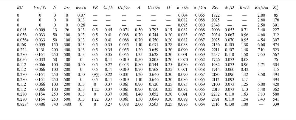


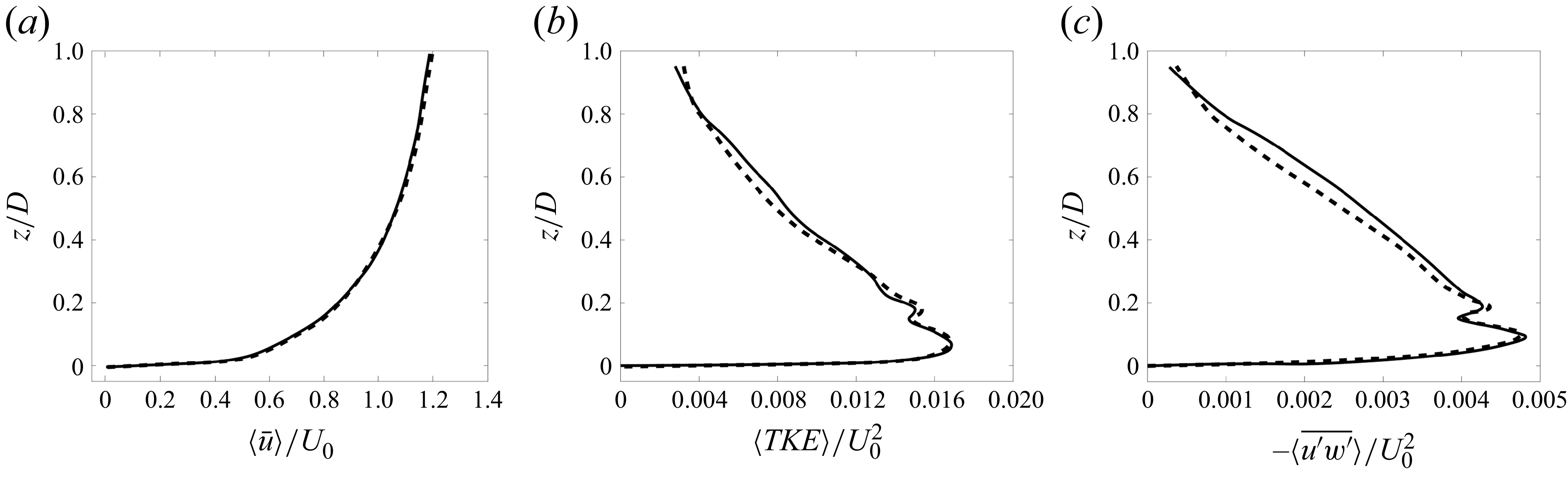

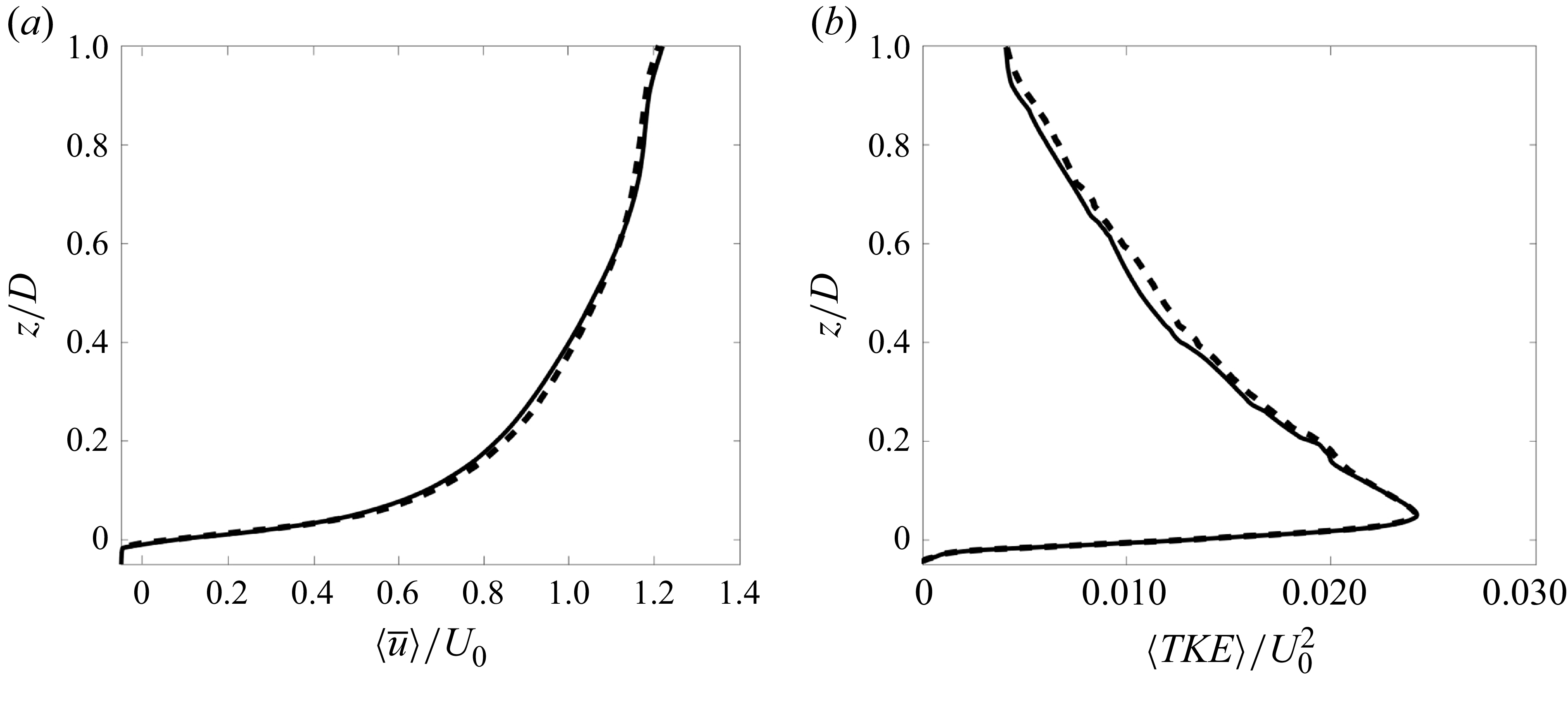


 Open access