


1. Introduction
Nowadays, shock models are widely adopted for the description of lifetimes of systems working in random environments in various fields, including survival analysis, reliability engineering, insurance and finance (see Cha and Finkelstein [Reference Cha and Finkelstein13]). In the literature, the existing shock models can be classified into five classes: (1) extreme shock models, where a system fails due to a single shock whose magnitude exceeds a fixed threshold (see, for instance, Cha and Finkelstein [Reference Cha and Finkelstein9, Reference Cha and Finkelstein11]); (2) cumulative shock models, in which a system fails when the cumulative damage caused by shocks exceeds a given threshold (see Gut [Reference Gut23] and Wang [Reference Wang38]); (3) run shock models, in which the failure of the system happens when the magnitudes of a given number of consecutive shocks are greater than a certain threshold (Mallor and Omey [Reference Mallor and Omey28]; Ozkut [Reference Ozkut and Eryilmaz31] and Eryilmaz [Reference Eryılmaz17]); (4) δ-shock models, where we observe the failure of the device when the time between two consecutive shocks is less than a fixed threshold value δ (see Goyal, Hazra and Finkelstein [Reference Goyal, Hazra and Finkelstein20]; Eryilmaz [Reference Eryilmaz16]; Jiang [Reference Jiang25]; Li, Chan and Yuan [Reference Li, Chan and Yuan27]); (5) mixed shock models, in which different kinds of shock models are combined (see Wang and Zhang [Reference Wang and Zhang39]). Other more general shock models have been studied over the last years: see, for instance, Belzunce et al. [Reference Belzunce, Lillo, Pellerey and Shaked4] for the case of multivariate shock models, Cha and Badía [Reference Cha and Badí8] for stochastically dependent dynamic shock models and Mallor and Santos [Reference Mallor and Santos29] for a general shock model which includes a correlation structure.
A customary assumption in shock models is that the stochastic process governing the arrival of shocks is a homogeneous or a non-homogeneous Poisson process (see, for instance, Grandell [Reference Grandell21]). The latter counting processes are both characterized by independent increments, this resulting in a high mathematical tractability of the model (see, for instance, Pellerey, Shaked, and Zinn [Reference Pellerey, Shaked and Zinn32] for some results concerning the epoch times and the inter-epoch intervals of a non-homogeneous Poisson process). However, this assumption seems unrealistic in many applications and, for this reason, some authors proposed different stochastic processes to model the occurrence of shocks. In particular, in the work by Eryilmaz [Reference Eryilmaz16], the δ-shock model is treated under the assumptions of shocks arriving according to a Pòlya process, i.e., a mixed Poisson process with mixing distribution given by a gamma probability density function. Furthermore, a generalized Pòlya process has been considered in Konno [Reference Konno26] and Cha [Reference Cha7], whereas in Di Crescenzo and Pellerey [Reference Di Crescenzo and Pellerey15] the authors consider a geometric counting process governing the arrivals of shocks.
In the present manuscript we propose a mixed Poisson process with inverse gamma mixing distribution to describe the arrivals of shocks. As mentioned by Willmot [Reference Willmot41], mixed Poisson processes are often used for modeling claim counts but, with the exception of few cases, they are difficult to be evaluated, this limiting their use. On the contrary, the counting process proposed in the present manuscript, named the inverse gamma mixed Poisson (IGMP) process, is characterized by a high mathematical tractability. In particular, the IGMP process shares with the Pòlya process the three characteristics stated in Beichelt [Reference Beichelt3]: both processes have (1) explicitly available finite dimensional distributions, (2) dependent increments, (3) free parameters allowing the model adaptation to a wide variety of data sets. Moreover, since the model properties arise from the choice of an inverse gamma mixing distribution, the IGMP process lends itself to being used in situations in which the underlying counting rate is better characterized by an inverse gamma distribution.
The inverse gamma distribution is one of the most useful distributions for describing different physical scenarios. For instance, in modeling shadow fading, the inverse gamma distribution is considered as an alternative to the gamma distribution since it admits a relatively simple mathematical formulation and exhibits heavy-tailed characteristics similar to the gamma density. The role of the inverse gamma distribution in describing the random variation of the mean signal power in composite fading channels is described in Yoo et al. [Reference Yoo, Simmons, Cotton, Sofotasios, Matthaiou, Valkama and Karagiannidis44], whereas an empirical validation of the inverse gamma distribution for modeling shadowing is provided in Yoo et al. [Reference Yoo, Cotton, Zhang and Sofotasios43]. The use of the inverse gamma as a survival distribution is discussed in Glen [Reference Glen19], in which its upside-down bathtub (UBT) shaped hazard function is pinpointed. See also Ramirez-Espinosa and Lopez-Martinez [Reference Ramiırez-Espinosa and Lopez-Martinez35] for a discussion concerning the benefits brought by the inverse gamma distribution to model shadowing, or Mead [Reference Mead30] for applications of such distribution in corrosion problems in new machines. The discretized form of the inverse gamma distribution has been recently proposed by Pundir et al. [Reference Pundir, Srivastava, Agarwal and Shrivastava34] as a suitable lifetime model.
Section 2 provides the main properties of the IGMP process. Similarly to other mixed Poisson processes, the inverse gamma mixed Poisson process is overdispersed. However, by analyzing the limit behavior of the coefficient of variation, the IGMP process, as time increases, tends to become qualitatively more regular than a Poisson process.
The distribution of the arrival time of the kth shock and that of the interarrival time between consecutive shock arrivals are also obtained in Section 2. In particular, we prove that the interarrival times follow the so-called K-distribution, which is characterized by heavy tails. This means that there is a high probability of observing long interarrival times and that the density does not decay rapidly. This property is shared by the Pòlya process, for which the interarrival times follow the Pareto distribution. However, the mean interarrival time of the Pòlya process can be infinite when the tail parameter is less than or equal to 1. On the contrary, the K-distribution typically has a finite mean and this property can be advantageous in applications where it is necessary to estimate or predict the average time between occurrences.
Throughout the manuscript, we consider three classes of shock models under the assumption of an IGMP process governing the arrival of shocks. In particular, in Section 3 we obtain the survival function for the extreme shock model, the δ-shock model and the cumulative shock model. In the latter case, we assume an exponentially distributed random threshold and consider different choices of the distribution of the random variable representing the amount of damage caused by the kth shock. We show that the IGMP process owns the weak positive dependence property, this meaning that the absence of shocks in a fixed time interval decreases the probability of a shock in the next short interval of time. Such property, which is shared by other processes such as the conditional Poisson process or the Geometric Counting Process (see Cha and Finkelstein [Reference Cha and Finkelstein11]), eventually results in decreasing the failure rate. Indeed, both in the extreme and cumulative shock model (for an exponentially distributed random threshold) we prove that the system failure time is characterized by a decreasing failure rate. Hence, the probability of a failure in a fixed time interval in the future decreases over time, thus suggesting that the system improves as time goes on. This property provides a crucial distinction of the IGMP shock model from other well-known shock models for which the failure rate usually exhibits an increasing behavior. For instance, for an extreme shock model with constant system’s failure probability, under the assumption of shocks governed by a generalized Pòlya process with constant baseline function, the failure rate function exhibits an increasing behavior (see Cha and Finkelstein [Reference Cha and Finkelstein12]).
Finally, in order to highlight the practical use of the process in applications, in Appendix A.1 we propose some examples of real data fitting. In particular, we conduct a chi-square goodness of fit test to determine if the observed frequency distribution fits the IGMP distribution. The first dataset concerns the occurrences of earthquakes in Italy from 1,961 to 2,018; the second one describes the number of hourly vessel arrivals at the Hong Kong Port during May 2014.
It is worth pointing out that, as a byproduct of our investigations, in Sections 2 and 3 we obtain some results concerning the sum of series of modified Bessel functions of the second kind which have not been given before, to the best of our knowledge.
2. The inverse gamma mixed Poisson process
Let N(t) be a mixed Poisson process (MPP) with marginal distribution:
 \begin{equation}
\eta_k(t):=\mathbb{P}[N(t)=k]=\int_{0}^{\infty}\mathbb{P}[N^{(\lambda)}(t)=k] {\rm d}U(\lambda), \quad k \in \mathbb{N},\ t \geq 0,
\end{equation}
\begin{equation}
\eta_k(t):=\mathbb{P}[N(t)=k]=\int_{0}^{\infty}\mathbb{P}[N^{(\lambda)}(t)=k] {\rm d}U(\lambda), \quad k \in \mathbb{N},\ t \geq 0,
\end{equation} where  $N^{(\lambda)}(t)$ is a Poisson process with intensity λ > 0 and $U(\cdot)$ is an inverse gamma distribution defined on $\mathbb{R}^{+}_0$ with density:
 \begin{equation}
dU(\lambda)=\textbf{1}_{\{\lambda \gt 0\}} \frac{1}{\Gamma(\alpha)}\frac{\beta^{\alpha}}{\lambda^{\alpha+1}} e^{-\beta/\lambda} {\rm d} \lambda, \quad \alpha \gt 0, \beta \gt 0.
\end{equation}
\begin{equation}
dU(\lambda)=\textbf{1}_{\{\lambda \gt 0\}} \frac{1}{\Gamma(\alpha)}\frac{\beta^{\alpha}}{\lambda^{\alpha+1}} e^{-\beta/\lambda} {\rm d} \lambda, \quad \alpha \gt 0, \beta \gt 0.
\end{equation}We shall call N(t) the inverse gamma mixed Poisson (IGMP) process and, for t > 0, the expression of its probability distribution is given by (see Willmot [Reference Willmot41])
 \begin{equation}
\eta_k(t)=\frac{2}{k!\, \Gamma(\alpha)}\big(\beta t\big)^{\frac{\alpha+k}{2}}K_{\alpha-k}(2\sqrt{\beta t}),\qquad k=0,1,2,\ldots,
\end{equation}
\begin{equation}
\eta_k(t)=\frac{2}{k!\, \Gamma(\alpha)}\big(\beta t\big)^{\frac{\alpha+k}{2}}K_{\alpha-k}(2\sqrt{\beta t}),\qquad k=0,1,2,\ldots,
\end{equation} where  $K_{v}(\cdot)$ is the modified Bessel function of the second kind, defined as:
 \begin{equation}
K_{v}(w)=\frac{1}{2}\int_{0}^{\infty}x^{v-1}e^{-{\frac{w}{2}\big(x+\frac{1}{x}\big)}}{\rm d}x, \quad \nu \in \mathbb{R}, \ w \gt 0.
\end{equation}
\begin{equation}
K_{v}(w)=\frac{1}{2}\int_{0}^{\infty}x^{v-1}e^{-{\frac{w}{2}\big(x+\frac{1}{x}\big)}}{\rm d}x, \quad \nu \in \mathbb{R}, \ w \gt 0.
\end{equation} Some plots of the probability distribution  $\eta_k(t)$ are shown in Figure 1 for different values of t.
Plot of  $\eta_k(t)$ for α = 0.5, β = 1 with t = 0.1 (on the left) and t = 1 (on the right).

Remark 2.1. We recall that, according to well-known properties of mixed Poisson processes (see for instance, Rolski et al. [Reference Rolski, Schmidli, Schmidt and Teugels36]), the probabilities  $\eta_k(t)$ for $k=1,2,\ldots,$ can be expressed in terms of the zero-state probability $\eta_0(t)$. Indeed, the function $\eta_0(t)$ is infinitely often differentiable such that:
 \begin{equation}
\eta_k(t)=(-1)^k \frac{t^k}{k!}\ \eta^{(k)}_0(t), \quad t \geq 0, \ k \in \mathbb{N},
\end{equation}
\begin{equation}
\eta_k(t)=(-1)^k \frac{t^k}{k!}\ \eta^{(k)}_0(t), \quad t \geq 0, \ k \in \mathbb{N},
\end{equation}where
 \begin{equation*}
\eta^{(k)}_0(t):=\frac{\partial^k}{\partial t^k}\eta_0(t)=(-1)^k \int_0^{\infty} \lambda^k e^{-\lambda t} {\rm d}U(\lambda).
\end{equation*}
\begin{equation*}
\eta^{(k)}_0(t):=\frac{\partial^k}{\partial t^k}\eta_0(t)=(-1)^k \int_0^{\infty} \lambda^k e^{-\lambda t} {\rm d}U(\lambda).
\end{equation*} Recalling Eq. (1), it immediately follows that, for each  $t \geq 0$,
 \begin{equation*}
\sum_{k=0}^{\infty} \eta_k(t)=1.
\end{equation*}
\begin{equation*}
\sum_{k=0}^{\infty} \eta_k(t)=1.
\end{equation*}As a byproduct of this result, the following corollary shows a simple relation involving the gamma function and a series of modified Bessel functions, which does not appear to have been given before.
Corollary 2.1. For α > 0 and z > 0 we have
 \begin{equation*}
\sum_{n=0}^{\infty} \frac{1}{n!}\left(\frac{z}{2}\right)^{n} K_{\alpha-n}(z) =
\frac{\Gamma(\alpha)}{z^\alpha} \cdot 2^{\alpha-1}.
\end{equation*}
\begin{equation*}
\sum_{n=0}^{\infty} \frac{1}{n!}\left(\frac{z}{2}\right)^{n} K_{\alpha-n}(z) =
\frac{\Gamma(\alpha)}{z^\alpha} \cdot 2^{\alpha-1}.
\end{equation*}The following Proposition provides some results concerning the IGMP process, which immediately follow from the properties of the mixed Poisson process (see, for instance, Rolski et al. [Reference Rolski, Schmidli, Schmidt and Teugels36] or Grandell [Reference Grandell21]). To the best of our knowledge, the IGMP process has never been studied in detail in the literature.
Proposition 2.1. Let N(t) be an inverse gamma mixed Poisson process. Then, for t > 0, the following properties hold:
(i) N(t) admits stationary increments, i.e., for $\alpha, \beta \gt 0$, $n=1,2,\ldots$ and each sequence $\{k_r; r=1,\ldots,n\}$ of nonnegative integers, it is:
(6)\begin{eqnarray}
&& \hspace{-2.7cm}
P\left( \bigcap\limits_{r=1}^{n} \{N(b_r)-N(a_r)=k_r\}\right)=\prod_{r=1}^{n} \frac{(b_r-a_r)^{k_r}}{k_r!}
\nonumber\\
&& \hspace{2.6cm}
\times
\frac{2 \beta^{\frac{\alpha+k}{2}} \left[\sum_{r=1}^n (b_r-a_r) \right]^{\frac{\alpha-k}{2}}
K_{\alpha-k}(2 \sqrt{\beta \sum_{r=1}^n (b_r-a_r)})}{\Gamma(\alpha)},
\end{eqnarray}
$\alpha, \beta \gt 0$, $n=1,2,\ldots$ and each sequence $\{k_r; r=1,\ldots,n\}$ of nonnegative integers, it is:
(6)\begin{eqnarray}
&& \hspace{-2.7cm}
P\left( \bigcap\limits_{r=1}^{n} \{N(b_r)-N(a_r)=k_r\}\right)=\prod_{r=1}^{n} \frac{(b_r-a_r)^{k_r}}{k_r!}
\nonumber\\
&& \hspace{2.6cm}
\times
\frac{2 \beta^{\frac{\alpha+k}{2}} \left[\sum_{r=1}^n (b_r-a_r) \right]^{\frac{\alpha-k}{2}}
K_{\alpha-k}(2 \sqrt{\beta \sum_{r=1}^n (b_r-a_r)})}{\Gamma(\alpha)},
\end{eqnarray}where
$k=\sum_{r=1}^n k_r$ and $0 \lt a_1\leq b_1\leq a_2\leq b_2\leq\ldots\leq a_n\leq b_n$.(ii) For
$r \in \mathbb{N}$, $\alpha \gt r$, β > 0, the rth factorial moment of N(t) is:
\begin{equation*}
\mathbb{E}[(N(t))_r]:=\mathbb{E}[N(t)(N(t)-1)\ldots(N(t)-r+1)]=\frac{(\beta t)^r}{(\alpha-1)\cdots(\alpha-r)}.
\end{equation*}In particular, the expected value and the variance of N(t) are given by:
(7)\begin{equation}
\mathbb{E}[N(t)]=\frac{\beta t}{\alpha-1}, \quad \alpha \gt 1 , \quad \text{Var}[N(t)]=\frac{(\beta t)^2}{(\alpha-1)^2(\alpha-2)}+\frac{\beta t}{\alpha-1}, \quad \alpha \gt 2.
\end{equation}(iii) For
$\alpha \gt 2, \beta \gt 0$ and h > 0, it results
(8)\begin{equation}
Cov[N(t), N(t + h)-N(t)] = \frac{\beta^2 t\, h}{(\alpha-1)^2(\alpha-2)}.
\end{equation}(iv) For
$\alpha, \beta \gt 0$, the probability generating function of N(t) is given by:
(9)\begin{equation}
G_{N(t)}(z):=\mathbb{E}[z^{N(t)}]=\frac{2}{\Gamma(\alpha)}[\beta t(1-z)]^{\frac{\alpha}{2}} K_{\alpha}(2\sqrt{\beta t(1-z)}),\qquad |z| \lt 1.
\end{equation}


Remark 2.2. From Eq. (7) we note that, for all t > 0,  $\text{Var}[N(t)] \gt \mathbb{E}[N(t)]$, thus implying that the IGMP process is overdispersed. However, for α > 2, the coefficient of variation of N(t) at time t > 0 is given by:
 \begin{equation*}
CV_t:=\frac{\sqrt{\text{Var}[N(t)]}}{\mathbb{E}[N(t)]}
=\sqrt{\frac{\alpha-1}{\beta t}+\frac{1}{\alpha-2}},
\end{equation*}
\begin{equation*}
CV_t:=\frac{\sqrt{\text{Var}[N(t)]}}{\mathbb{E}[N(t)]}
=\sqrt{\frac{\alpha-1}{\beta t}+\frac{1}{\alpha-2}},
\end{equation*}so that
 \begin{equation*}
\lim_{t\rightarrow +\infty} CV_t=\frac{1}{\sqrt{\alpha-2}}.
\end{equation*}
\begin{equation*}
\lim_{t\rightarrow +\infty} CV_t=\frac{1}{\sqrt{\alpha-2}}.
\end{equation*}Hence, the coefficient of variation is decreasing in t, and it is less than one for large t. This suggests that the IGMP process, as time increases, tends to become qualitatively more regular than a Poisson process.
Remark 2.3. From Eq. (8) we can deduce that adjacent increments of N(t) are positively correlated for α > 2. Hence, for the IGMP process, a large number of events in a given time interval tends to lead to a large number of events in the next interval.
In the following Theorem we prove that the IGMP process owns the weak positive dependence property. We recall that a counting process  $\{M(t), \; t \geq 0\}$ satisfies the weak positive dependence property if
 \begin{equation}
\mathrm{Cov} \left(I(\{M(s+t)-M(s)=0 \}), I(\{M(s)=0\}\right) \gt 0,
\end{equation}
\begin{equation}
\mathrm{Cov} \left(I(\{M(s+t)-M(s)=0 \}), I(\{M(s)=0\}\right) \gt 0,
\end{equation} where  $s,t \gt 0$ and I(E) represents the indicator function for the event E (see, for instance, Cha and Finkelstein [Reference Cha and Finkelstein11]).
Theorem 2.1. The IGMP process has the weak positive dependence property.
Proof. Due to Eq. (10), the IGMP satisfies the weak positive dependence property if the inequality:
 \begin{equation}
P(N(s+t)-N(s)=0, N(s)=0)-P(N(s+t)-N(s)=0)P(N(s)=0) \gt 0,
\end{equation}
\begin{equation}
P(N(s+t)-N(s)=0, N(s)=0)-P(N(s+t)-N(s)=0)P(N(s)=0) \gt 0,
\end{equation} holds for any  $s, t\in {\mathbb R}^+$. Due to Proposition 6 and recalling Eq. (1), Eq. (11) reads:
 \begin{equation}
\frac{2}{\Gamma(\alpha)} (\beta (s+t))^{\frac{\alpha}{2}} K_{\alpha} (2 \sqrt{\beta(s+t)})-\frac{2}{\Gamma(\alpha)} (\beta s)^{\frac{\alpha}{2}} K_{\alpha} (2 \sqrt{\beta s}) \, \frac{2}{\Gamma(\alpha)} (\beta t)^{\frac{\alpha}{2}} K_{\alpha} (2 \sqrt{\beta t}) \gt 0.
\end{equation}
\begin{equation}
\frac{2}{\Gamma(\alpha)} (\beta (s+t))^{\frac{\alpha}{2}} K_{\alpha} (2 \sqrt{\beta(s+t)})-\frac{2}{\Gamma(\alpha)} (\beta s)^{\frac{\alpha}{2}} K_{\alpha} (2 \sqrt{\beta s}) \, \frac{2}{\Gamma(\alpha)} (\beta t)^{\frac{\alpha}{2}} K_{\alpha} (2 \sqrt{\beta t}) \gt 0.
\end{equation}In order to prove this inequality, we define the functions:
 \begin{equation}
f(x):=\frac{2}{\Gamma(\alpha)}(\sqrt{x})^{\alpha} K_{\alpha}(2\sqrt{x}), \qquad g(x):=\frac{1}{f(x)}, \qquad x \gt 0,
\end{equation}
\begin{equation}
f(x):=\frac{2}{\Gamma(\alpha)}(\sqrt{x})^{\alpha} K_{\alpha}(2\sqrt{x}), \qquad g(x):=\frac{1}{f(x)}, \qquad x \gt 0,
\end{equation}where recalling that (see Gaunt [Reference Gaunt18]):
 \begin{equation*}
2^{\nu - 1}\Gamma(\nu)e^{- x} \lt x^{\nu}K_{\nu}(x) \lt 2^{\nu - 1}\Gamma(\nu),\qquad x \gt 0, \nu \gt 0,
\end{equation*}
\begin{equation*}
2^{\nu - 1}\Gamma(\nu)e^{- x} \lt x^{\nu}K_{\nu}(x) \lt 2^{\nu - 1}\Gamma(\nu),\qquad x \gt 0, \nu \gt 0,
\end{equation*} it results  $0 \lt f(x) \lt 1$ and $g(x) \gt 1$, $\forall x \gt 0$. Due to the above assumptions, the proof of Eq. (12) can be obtained by showing that, for $x,h \gt 0$, one has
 \begin{equation*}
g(x+h) \lt g(x)\cdot g(h),
\end{equation*}
\begin{equation*}
g(x+h) \lt g(x)\cdot g(h),
\end{equation*} with  $g(0)=1$, being (see, for instance, Abramowitz and Stegun [Reference Abramowitz and Stegun1]):
 \begin{equation}
K_{\nu}(x) \sim \frac{1}{2} \Gamma(\nu)\left( \frac{1}{2} x \right)^{-\nu}, \quad x\rightarrow 0.
\end{equation}
\begin{equation}
K_{\nu}(x) \sim \frac{1}{2} \Gamma(\nu)\left( \frac{1}{2} x \right)^{-\nu}, \quad x\rightarrow 0.
\end{equation}For small h we have that
 \begin{equation*}
g(x+h) \lt g(x)g(h) \Leftrightarrow \frac{g'(x)}{g(x)} \lt \frac{g'(0)}{g(0)} \Leftrightarrow
\frac{\mathrm{d}}{\mathrm{d} x} \ln g(x) \Big\lvert_{x \gt 0} \lt \frac{\mathrm{d}}{\mathrm{d} x} \ln g(x) \Big\lvert_{x=0},
\end{equation*}
\begin{equation*}
g(x+h) \lt g(x)g(h) \Leftrightarrow \frac{g'(x)}{g(x)} \lt \frac{g'(0)}{g(0)} \Leftrightarrow
\frac{\mathrm{d}}{\mathrm{d} x} \ln g(x) \Big\lvert_{x \gt 0} \lt \frac{\mathrm{d}}{\mathrm{d} x} \ln g(x) \Big\lvert_{x=0},
\end{equation*} which means that the function  $\ln g(x)$ is concave, or, equivalently, $\ln f(x)$ is convex. This latter condition can be proved noting that due to a Turan-type inequality (see Baricz [Reference Baricz2]), for any positive α it results
 \begin{equation*}
K_{\alpha-1}^2(2\sqrt{x}) \leq K_{\alpha-2}(2\sqrt{x}) K_{\alpha}(2\sqrt{x}).
\end{equation*}
\begin{equation*}
K_{\alpha-1}^2(2\sqrt{x}) \leq K_{\alpha-2}(2\sqrt{x}) K_{\alpha}(2\sqrt{x}).
\end{equation*}Hence, being
 \begin{equation*}
\frac{f''(x)}{f(x)}-\left[ \frac{f'(x)}{f(x)}\right]^2 \geq 0 \Leftrightarrow f''(x) \geq \frac{[f'(x)]^2}{f(x)} \Leftrightarrow
x^{\frac{\alpha}{2}-1}K_{\alpha-2}(2\sqrt{x}) \geq \frac{x^{\alpha-1}K_{\alpha-1}^2 (2 \sqrt{x})}{x^{\frac{\alpha}{2}}K_{\alpha}(2\sqrt{x})},
\end{equation*}
\begin{equation*}
\frac{f''(x)}{f(x)}-\left[ \frac{f'(x)}{f(x)}\right]^2 \geq 0 \Leftrightarrow f''(x) \geq \frac{[f'(x)]^2}{f(x)} \Leftrightarrow
x^{\frac{\alpha}{2}-1}K_{\alpha-2}(2\sqrt{x}) \geq \frac{x^{\alpha-1}K_{\alpha-1}^2 (2 \sqrt{x})}{x^{\frac{\alpha}{2}}K_{\alpha}(2\sqrt{x})},
\end{equation*}the proof easily follows.
The following Proposition provides a further characterization of the IGMP process in terms of a suitable stochastic ordering. We recall that, given two discrete random variables Y and W, with discrete densities h and g, respectively, Y is said to be smaller than W in the likelihood ratio order,  $Y\leq_{lr} W$, if
 \begin{equation}
\frac{g(t)}{h(t)} \,\,\text{increases in}\, t\, \text{over the union of the supports of}\, Y \,\text{and}\, W,
\end{equation}
\begin{equation}
\frac{g(t)}{h(t)} \,\,\text{increases in}\, t\, \text{over the union of the supports of}\, Y \,\text{and}\, W,
\end{equation}(see, for instance, Belzunce, Martinez Riquelme and Mulero [Reference Belzunce, Martinez Riquelme and Mulero5]). We recall that stochastic orders allow to compare probability distributions or measures and represent a powerful tool used in many areas such as reliability, survival analysis, risks, finance, and economics. In particular, the likelihood ratio order is stronger than other orderings, such as the stochastic order, this justifying the goal of exploring its validity.
Proposition 2.2. Let N(t) be a IGMP process. Then, for  $\alpha,\beta \gt 0$, N(t) increases in the likelihood ratio order when t increases.
Proof. We aim to show that for  $0 \lt s \lt t$, it is $N(s)\leq_{lr} N(t)$, i.e., due to Eq. (15), the ratio $\frac{P(N(t)=n)}{P(N(s)=n)}$ is increasing with respect to n.
Being (see Eq. (3))
 \begin{equation*}
\frac{P(N(t)=n)}{P(N(s)=n)}=\Big({\frac{t}{s}}\Big)^{n/2}\, \frac{K_{n-\alpha}(2 \sqrt{\beta t})}{K_{n-\alpha}(2 \sqrt{\beta s})},
\end{equation*}
\begin{equation*}
\frac{P(N(t)=n)}{P(N(s)=n)}=\Big({\frac{t}{s}}\Big)^{n/2}\, \frac{K_{n-\alpha}(2 \sqrt{\beta t})}{K_{n-\alpha}(2 \sqrt{\beta s})},
\end{equation*} we have to show that, for  $n\in {\mathbb N}$, it is
 \begin{equation*}
2 \sqrt{\beta s}\, \frac{K_{n+1-\alpha}(2 \sqrt{\beta s})}{K_{n-\alpha}(2 \sqrt{\beta s})}\leq 2 \sqrt{\beta t}\,\frac{K_{n+1-\alpha}(2 \sqrt{\beta t})}{K_{n-\alpha}(2 \sqrt{\beta t})},
\end{equation*}
\begin{equation*}
2 \sqrt{\beta s}\, \frac{K_{n+1-\alpha}(2 \sqrt{\beta s})}{K_{n-\alpha}(2 \sqrt{\beta s})}\leq 2 \sqrt{\beta t}\,\frac{K_{n+1-\alpha}(2 \sqrt{\beta t})}{K_{n-\alpha}(2 \sqrt{\beta t})},
\end{equation*}i.e. the function
 \begin{equation*}
h(z):=z\, \frac{K_{n+1-\alpha}(z)}{K_{n-\alpha}(z)}
\end{equation*}
\begin{equation*}
h(z):=z\, \frac{K_{n+1-\alpha}(z)}{K_{n-\alpha}(z)}
\end{equation*}is increasing with respect to z. Noting that, due to Eq. (9.6) of Abramowitz and Stegun [Reference Abramowitz and Stegun1],
 \begin{equation*}
h(z)=z\, \frac{K_{n-1-\alpha}(z)}{K_{n-\alpha}(z)}+2 (n-\alpha),
\end{equation*}
\begin{equation*}
h(z)=z\, \frac{K_{n-1-\alpha}(z)}{K_{n-\alpha}(z)}+2 (n-\alpha),
\end{equation*}the proof immediately follows from Eq. (2.2) of Yang and Zheng [Reference Yang and Zheng42].
2.1. Distribution of arrival and interarrival times
For the IGMP process, let us denote by Tk,  $k \in \mathbb{N}^+$, the arrival time of the kth event and by $X_k = T_k - T_{k-1}$, $k \in \mathbb{N}^+$ $(T_0 = 0)$, the interarrival time between consecutive events.
The explicit expression of the distribution of Tk is provided in the following theorem.
Theorem 2.2. For t > 0 and  $k \in \mathbb{N}^+$, we have
 \begin{eqnarray}
&& \hspace{-1cm}
F_{T_k}(t):=P(T_k\leq t)=1-\frac{2}{\Gamma(\alpha)}(\sqrt{\beta t})^{\alpha}\sum_{i=0}^{k-1}\frac{(\sqrt{\beta t})^i}{i!}K_{\alpha-i}(2\sqrt{\beta t}),\nonumber\\
&& \hspace{-1cm}
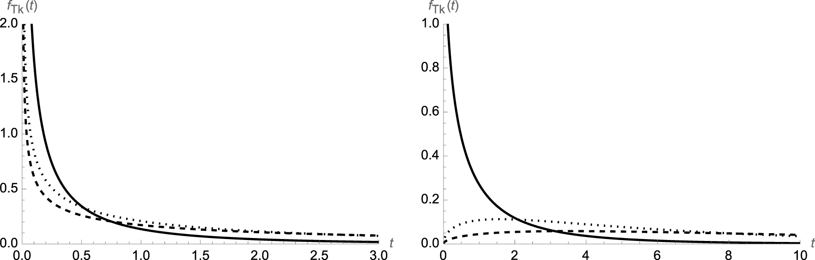
f_{T_k}(t):= \frac{{\rm d}}{{\rm d} t}P(T_k\leq t)=\frac{2}{(k-1)! \Gamma(a)} \beta^{\frac{\alpha+k}{2}} t^{\frac{\alpha+k}{2}-1} K_{\alpha-k}(2\sqrt{\beta t}),
\end{eqnarray}
\begin{eqnarray}
&& \hspace{-1cm}
F_{T_k}(t):=P(T_k\leq t)=1-\frac{2}{\Gamma(\alpha)}(\sqrt{\beta t})^{\alpha}\sum_{i=0}^{k-1}\frac{(\sqrt{\beta t})^i}{i!}K_{\alpha-i}(2\sqrt{\beta t}),\nonumber\\
&& \hspace{-1cm}
f_{T_k}(t):= \frac{{\rm d}}{{\rm d} t}P(T_k\leq t)=\frac{2}{(k-1)! \Gamma(a)} \beta^{\frac{\alpha+k}{2}} t^{\frac{\alpha+k}{2}-1} K_{\alpha-k}(2\sqrt{\beta t}),
\end{eqnarray}Proof. Recalling that  $\{N(t) \geq k\}= \{T_k \leq t\}$ for all $t \geq 0$, the proof immediately follows from Eq. (3).
Some plots of the probability density (16) are shown in Figure 2 for different values of the parameters α and β and for different choices of k.
Plot of  $f_{T_k}(t)$ for β = 1 and k = 1 (solid line), k = 5 (dotted line) and k = 9 (dashed line) with α = 0.5 (on the left) and α = 1.5 (on the right).
In the next proposition we obtain the joint distribution of the arrival epochs Tk:
Proposition 2.3. The joint density of the vector  $T=(T_1, \ldots, T_m)$, for $(t_1, \ldots,t_m) \in \mathbb{R}^m$ such that $0 \lt t_1 \lt \ldots \lt t_m$, is given by:
 \begin{equation}
f_{T}(t_1, \ldots,t_m):=\frac{\partial^m}{\partial t_1\cdots \partial t_m} P(T_1\leq t_1,\ldots,T_m\leq t_m)
=\frac{2}{\Gamma(\alpha)}t_m^{\frac{\alpha-m}{2}} \beta^{\frac{\alpha+m}{2}} K_{\alpha-m}\big(2\sqrt{\beta t_m}\big).
\end{equation}
\begin{equation}
f_{T}(t_1, \ldots,t_m):=\frac{\partial^m}{\partial t_1\cdots \partial t_m} P(T_1\leq t_1,\ldots,T_m\leq t_m)
=\frac{2}{\Gamma(\alpha)}t_m^{\frac{\alpha-m}{2}} \beta^{\frac{\alpha+m}{2}} K_{\alpha-m}\big(2\sqrt{\beta t_m}\big).
\end{equation}Proof. Recalling Theorem 5.2 of Chapter VIII in Rolski et al. [Reference Rolski, Schmidli, Schmidt and Teugels36], we have that
 \begin{equation*}
f_{T}(t_1, \ldots,t_m)=\frac{m!}{t^m_m} P(N(t_m)=m).
\end{equation*}
\begin{equation*}
f_{T}(t_1, \ldots,t_m)=\frac{m!}{t^m_m} P(N(t_m)=m).
\end{equation*}Some properties of the interarrival times are disclosed in the following propositions.
Let us denote by  $\boldsymbol{X}_m=(X_1, X_2, \ldots, X_m)$ the vector of the interarrival times of the IGMP process.
Proposition 2.4. For  $x_1, x_2, \ldots, x_m \gt 0$ we have
 \begin{eqnarray*}
&& \hspace{-1.5cm}
f_{\boldsymbol{X}_m}(x_1,x_2, \ldots,x_m):=\frac{\partial}{\partial x_1\cdots \partial x_m} P(X_1\leq x_1,\ldots,X_m\leq x_m)
\nonumber\\
&& \hspace{-1.5cm}
=\frac{2}{\Gamma(\alpha)}(x_1+x_2+ \ldots+ x_m)^{\frac{\alpha-m}{2}}\beta^{\frac{\alpha+m}{2}}K_{\alpha-m}\bigg(2\sqrt{\beta (x_1+x_2+ \ldots+ x_m)}\bigg).
\end{eqnarray*}
\begin{eqnarray*}
&& \hspace{-1.5cm}
f_{\boldsymbol{X}_m}(x_1,x_2, \ldots,x_m):=\frac{\partial}{\partial x_1\cdots \partial x_m} P(X_1\leq x_1,\ldots,X_m\leq x_m)
\nonumber\\
&& \hspace{-1.5cm}
=\frac{2}{\Gamma(\alpha)}(x_1+x_2+ \ldots+ x_m)^{\frac{\alpha-m}{2}}\beta^{\frac{\alpha+m}{2}}K_{\alpha-m}\bigg(2\sqrt{\beta (x_1+x_2+ \ldots+ x_m)}\bigg).
\end{eqnarray*}Proof. Due to Theorem 5.3 of Chapter VIII in Rolski et al. [Reference Rolski, Schmidli, Schmidt and Teugels36], it is:
 \begin{equation*}
f_{\boldsymbol{X}_m}(x_1,x_2, \ldots,x_m)=(-1)^m \eta_0^{(m)}(x_1+x_2+ \ldots+ x_m),
\end{equation*}
\begin{equation*}
f_{\boldsymbol{X}_m}(x_1,x_2, \ldots,x_m)=(-1)^m \eta_0^{(m)}(x_1+x_2+ \ldots+ x_m),
\end{equation*} where  $\eta_0^{(m)}$ is defined in Eq. (5). Hence the proof follows by making use of straightforward calculations.
As an immediate consequence of Proposition 2.4, we obtain the marginal density of the interarrival times Xk,  $k\in \mathbb{N}^+$.
Proposition 2.5. For all x > 0,  $k\in \mathbb{N}^+$, the marginal density of the interarrival times Xk is given by:
 \begin{equation}
f_{X_k}(x) =\frac{2\beta}{\Gamma(\alpha)} \big(\beta\,x\big)^{\frac{\alpha-1}{2}}K_{\alpha-1}\big(2\sqrt{\beta x}\big).
\end{equation}
\begin{equation}
f_{X_k}(x) =\frac{2\beta}{\Gamma(\alpha)} \big(\beta\,x\big)^{\frac{\alpha-1}{2}}K_{\alpha-1}\big(2\sqrt{\beta x}\big).
\end{equation} The density (18) is the so-called K-distribution (see Ward, Watts and Tough [Reference Ward, Tough and Watts40]) where α is the shape factor, β is the scale factor, and  $K_\nu(\cdot)$ is the modified Bessel function of second kind defined in Eq. (4).
Starting from Eq. (18), we provide the expression of the expected value and the variance of the interarrival times Xk,  $k\in \mathbb{N}^+$.
Corollary 2.2. For  $\alpha,\beta \gt 0$ and $k\in \mathbb{N}^+$, it results
 \begin{equation*}
E(X_k)=\frac{\alpha}{\beta},\qquad Var(X_k)=\frac{\alpha(\alpha+2)}{\beta^2}.
\end{equation*}
\begin{equation*}
E(X_k)=\frac{\alpha}{\beta},\qquad Var(X_k)=\frac{\alpha(\alpha+2)}{\beta^2}.
\end{equation*}Aiming to detect the dependence structure of the interarrival times Xk, in the following Proposition we evaluate the autocorrelation function, defined as:
 \begin{equation*}
\rho_i=\frac{Cov(X_j,X_{j+i})}{\sqrt{Var(X_j) Var(X_{j+i})}},\quad i=1,2,\ldots.
\end{equation*}
\begin{equation*}
\rho_i=\frac{Cov(X_j,X_{j+i})}{\sqrt{Var(X_j) Var(X_{j+i})}},\quad i=1,2,\ldots.
\end{equation*}Proposition 2.6. For α > 0, the autocorrelation function of the interarrival times is given by:
 \begin{equation}
\rho_i=\frac{1}{\alpha+2},\quad i=1,2,\ldots.
\end{equation}
\begin{equation}
\rho_i=\frac{1}{\alpha+2},\quad i=1,2,\ldots.
\end{equation}Proof. Recalling Eq. (4.6) of Cox and Lewis [Reference Cox and Lewis14], it is possible to evaluate the autocorrelation function as:
 \begin{equation}
\rho_i=E(X)\, \frac{\int_0^{+\infty} \tilde{p}(i,t) {\rm d}t -E(X)}{Var(X)},\quad i=1,2,\ldots,
\end{equation}
\begin{equation}
\rho_i=E(X)\, \frac{\int_0^{+\infty} \tilde{p}(i,t) {\rm d}t -E(X)}{Var(X)},\quad i=1,2,\ldots,
\end{equation}with
 \begin{equation}
\tilde{p}(i,t)=\frac{1}{i!} \frac{\partial^i}{\partial \xi^i}\left[1+\frac{(\xi-1)}{E(X)}\int_{0}^t G_{N(u)\!}(\xi)\, {\rm d}u \right]\Bigg \vert _{\xi=0},
\end{equation}
\begin{equation}
\tilde{p}(i,t)=\frac{1}{i!} \frac{\partial^i}{\partial \xi^i}\left[1+\frac{(\xi-1)}{E(X)}\int_{0}^t G_{N(u)\!}(\xi)\, {\rm d}u \right]\Bigg \vert _{\xi=0},
\end{equation} where  $G_{N(t)}(\cdot )$ is the probability generating function of the IGMP process, provided in Eq. (9).
Due to Eq. (9), and making use of straightforward calculations, we have that
 \begin{equation*}
1+\frac{(\xi-1)}{E(X)}\int_{0}^t G_{N(u)\!}(\xi)\, {\rm d}u=\frac{2}{\Gamma(\alpha+1)}[\beta t(1-\xi)]^{\frac{\alpha+1}{2}}K_{\alpha+1}(2 \sqrt{\beta t (1-\xi)}),
\end{equation*}
\begin{equation*}
1+\frac{(\xi-1)}{E(X)}\int_{0}^t G_{N(u)\!}(\xi)\, {\rm d}u=\frac{2}{\Gamma(\alpha+1)}[\beta t(1-\xi)]^{\frac{\alpha+1}{2}}K_{\alpha+1}(2 \sqrt{\beta t (1-\xi)}),
\end{equation*} which identifies with the probability generating function of a mixed Poisson process with mixing distribution given by an inverse gamma density with parameters  $(\alpha +1, \beta)$. Due to Eq. (21) and recalling Eq. (3), we thus have
 \begin{equation*}
\tilde{p}(i,t)=\frac{2}{i!\, \Gamma(\alpha+1)}\big(\beta t\big)^{\frac{\alpha+1+i}{2}}K_{\alpha+1-i}(2\sqrt{\beta t}),\qquad i=0,1,2,\ldots,\quad t \gt 0,
\end{equation*}
\begin{equation*}
\tilde{p}(i,t)=\frac{2}{i!\, \Gamma(\alpha+1)}\big(\beta t\big)^{\frac{\alpha+1+i}{2}}K_{\alpha+1-i}(2\sqrt{\beta t}),\qquad i=0,1,2,\ldots,\quad t \gt 0,
\end{equation*}so that
 \begin{equation*}
\int_0^{+\infty} \tilde{p}(i,t) {\rm d}t =\frac{\alpha+1}{\beta}.
\end{equation*}
\begin{equation*}
\int_0^{+\infty} \tilde{p}(i,t) {\rm d}t =\frac{\alpha+1}{\beta}.
\end{equation*}Hence, the proof immediately follows from Eq. (20) and recalling Corollary 2.2.
Note that the autocorrelation function (19) does not depend on the lag; this is in agreement with the stationarity of the interarrival times series.
3. Shock models
Let us consider a system subjected to external shocks that arrive according to the IGMP process, defined in Section 2. Due to the weak positive dependence (see Theorem 2.1), in this model the absence of shocks in a fixed time interval decreases the probability of a shock in the next short interval of time, this being common for some kind of shock processes. To the best of our knowledge, shock models governed by IGMP processes are new in the scientific landscape and they represent an alternative to the well-known Pòlya shock models.
Denoting by S the failure time of the system, we are interested in the study of the survival function and the rate function of S in three different cases: (i) extreme shock models (systems fail due to one single large shock), (ii) cumulative shock models (systems fail because of some cumulative effect) and (iii) δ-shock models (systems fail when the time between two consecutive shocks is less than a fixed value δ).
3.1. Extreme shock model
Let us consider the case in which the shocks occur independently and each one causes the failure of the system with the same probability  $p\in (0,1)$. Denoting by M the geometric random variable counting the number of shocks which cause the failure of the system, and by assuming M independent of N(t), for $t \geq 0$ we have:
 \begin{equation}
\overline{F}(t):=\mathbb{P}(S \gt t)=\sum_{k=0}^{\infty} \mathbb{P}(M \gt k) \eta_k(t)=\sum_{k=0}^{\infty} (1-p)^k \eta_k(t),
\end{equation}
\begin{equation}
\overline{F}(t):=\mathbb{P}(S \gt t)=\sum_{k=0}^{\infty} \mathbb{P}(M \gt k) \eta_k(t)=\sum_{k=0}^{\infty} (1-p)^k \eta_k(t),
\end{equation} where  $\eta_k(t)$ is defined in Eq. (1). Note that the assumption of independence between M and the process N(t) could be seen as restrictive in the description of real-world phenomena. Indeed, the occurrence of previous shocks could weaken the system, making it susceptible to further shocks (see, for instance, Cha and Finkelstein [Reference Cha and Finkelstein10], for a shock model based on a history-dependent approach). Such consideration could be regarded as the starting point for a future investigation.
The explicit forms of the survival probability and the expected value and variance of the failure time S are provided in the following theorem. In addition, the corresponding failure rate is also obtained.
Theorem 3.1. Let N(t) be the IGMP process. In the extreme shock model, the survival function of the system failure time S and the corresponding failure rate are given by:
 \begin{equation}
\overline{F}(t)=\frac{2}{\Gamma(\alpha)}(\sqrt{p\beta t})^{\alpha} K_{\alpha}(2\sqrt{p\beta t}),\quad t \geq 0,
\end{equation}
\begin{equation}
\overline{F}(t)=\frac{2}{\Gamma(\alpha)}(\sqrt{p\beta t})^{\alpha} K_{\alpha}(2\sqrt{p\beta t}),\quad t \geq 0,
\end{equation} \begin{equation}
r(t):=-\frac{{\rm d}\ln{\overline{F}(t)}}{{\rm d}t}=\sqrt{\frac{\beta p}{t}}\cdot \frac{K_{\alpha-1}(2\sqrt{p\beta t})}{K_{\alpha}(2\sqrt{p\beta t})},\quad t \gt 0.
\end{equation}
\begin{equation}
r(t):=-\frac{{\rm d}\ln{\overline{F}(t)}}{{\rm d}t}=\sqrt{\frac{\beta p}{t}}\cdot \frac{K_{\alpha-1}(2\sqrt{p\beta t})}{K_{\alpha}(2\sqrt{p\beta t})},\quad t \gt 0.
\end{equation}Moreover, the expected value and the variance of S are
 \begin{equation*}
\mathbb{E}(S)=\frac{\alpha}{p \beta},\qquad Var(S)=\frac{\alpha (\alpha+2)}{p^2 \beta^2}.
\end{equation*}
\begin{equation*}
\mathbb{E}(S)=\frac{\alpha}{p \beta},\qquad Var(S)=\frac{\alpha (\alpha+2)}{p^2 \beta^2}.
\end{equation*}Proof. Due to Eq. (22) and recalling Eq. (1), for  $t\geq 0$ and $0 \lt p \lt 1$, we have
 \begin{equation*}
\overline{F}(t)=G_{N(t)}(1-p),
\end{equation*}
\begin{equation*}
\overline{F}(t)=G_{N(t)}(1-p),
\end{equation*} where  $G_{N(t)}(z)$ is the probability generating function of the IGMP process (Eq. (9)).
The corresponding failure rate function is given by:
 \begin{equation*}
\begin{aligned}
r(t)&=-\frac{{\rm d}}{{\rm d} t}\bigg[\ln\bigg(\frac{2}{\Gamma(\alpha)}(\sqrt{p\beta t})^{\alpha} K_{\alpha}(2\sqrt{p\beta t})\bigg)\bigg]\\
&=-\bigg[\frac{\alpha}{2t}+\frac{p \beta\big(-K_{\alpha-1}(2\sqrt{p \beta t})-K_{\alpha+1}(2\sqrt{p \beta t})\big)}{2\sqrt{p \beta t}\,K_{\alpha}(2\sqrt{p \beta t})}\bigg], \quad t \gt 0.
\end{aligned}
\end{equation*}
\begin{equation*}
\begin{aligned}
r(t)&=-\frac{{\rm d}}{{\rm d} t}\bigg[\ln\bigg(\frac{2}{\Gamma(\alpha)}(\sqrt{p\beta t})^{\alpha} K_{\alpha}(2\sqrt{p\beta t})\bigg)\bigg]\\
&=-\bigg[\frac{\alpha}{2t}+\frac{p \beta\big(-K_{\alpha-1}(2\sqrt{p \beta t})-K_{\alpha+1}(2\sqrt{p \beta t})\big)}{2\sqrt{p \beta t}\,K_{\alpha}(2\sqrt{p \beta t})}\bigg], \quad t \gt 0.
\end{aligned}
\end{equation*} Being  $K_{\nu+1}(z)=\frac{2\nu}{z}K_{\nu}(z)+K_{\nu-1}(z)$ (see, for instance, Abramowitz and Stegun [Reference Abramowitz and Stegun1]), Eq. (24) follows after straightforward calculations. Finally, the expected value and the variance of S can be obtained from Eq. (23).
Remark 3.1. The failure rate (24) is decreasing for all t > 0 and tends to zero as t goes to infinity. This result immediately follows from the Hankel’s expansion for the modified Bessel function of the second kind (see Abramowitz and Stegun [Reference Abramowitz and Stegun1]), which, for sufficiently large z, reads:
 \begin{equation*}
K_{\nu}(z) \sim \left(\frac{\pi}{2z}\right)^{1/2} e^{-z} \sum_{k=0}^{\infty} \frac{(\frac{1}{2}-\nu)_k(\frac{1}{2}+\nu)_k}{(-2)^k \; k!}.
\end{equation*}
\begin{equation*}
K_{\nu}(z) \sim \left(\frac{\pi}{2z}\right)^{1/2} e^{-z} \sum_{k=0}^{\infty} \frac{(\frac{1}{2}-\nu)_k(\frac{1}{2}+\nu)_k}{(-2)^k \; k!}.
\end{equation*}As a byproduct of Theorem 3.1., recalling Eqs. (22) and (3), in Corollary 3.1 we obtain the explicit value of a series of modified Bessel functions of the second kind.
Corollary 3.1. For α > 0 and x > 0 we have
 \begin{equation*}
\sum_{k=0}^{\infty} \frac{(c \, x)^k}{k!} K_{\alpha-k}(x)= (1-2c)^\frac{\alpha}{2} K_{\alpha}(x \, \sqrt{1-2c}), \qquad 0\leq c \leq 1/2.
\end{equation*}
\begin{equation*}
\sum_{k=0}^{\infty} \frac{(c \, x)^k}{k!} K_{\alpha-k}(x)= (1-2c)^\frac{\alpha}{2} K_{\alpha}(x \, \sqrt{1-2c}), \qquad 0\leq c \leq 1/2.
\end{equation*}The following corollary provides the explicit expressions of the survival function and the rate function for a particular choice of α.
Corollary 3.2. Under the assumptions of Theorem 3.1, in the special case  $\alpha=1/2$ we have
 \begin{equation*}
\overline{F}(t)=e^{-2\sqrt{p\beta t}}, \quad r(t)=\sqrt{\frac{p \beta}{t}}, \quad t \gt 0.
\end{equation*}
\begin{equation*}
\overline{F}(t)=e^{-2\sqrt{p\beta t}}, \quad r(t)=\sqrt{\frac{p \beta}{t}}, \quad t \gt 0.
\end{equation*}Proof. It immediately follows from Theorem 3.1 recalling that
 \begin{equation*}
K_{\frac{1}{2}}(z)=\sqrt{\frac{\pi}{2z}}e^{-z}.
\end{equation*}
\begin{equation*}
K_{\frac{1}{2}}(z)=\sqrt{\frac{\pi}{2z}}e^{-z}.
\end{equation*}3.2. Cumulative shock model
Let us denote by Wk,  $k \in \mathbb{N}^+$, the random variable representing the amount of damage caused by the kth shock, whose arrival is governed by the IGMP process N(t). We assume that $\{W_k, k \in \mathbb{N}^+\}$ is a sequence of independent and identically distributed random variables with the distribution of the r.v. W, and that they are independent of N(t).
The total accumulated damage of the system from all shocks in  $[0,t)$ is given by:
 \begin{equation}
W(t)=\sum_{k=1}^{N(t)}W_k, \quad t \geq 0,
\end{equation}
\begin{equation}
W(t)=\sum_{k=1}^{N(t)}W_k, \quad t \geq 0,
\end{equation} where we make the customary assumption  $\sum_{k=1}^{0}W_k=0$.
The failure of the system occurs when the cumulative effect of shocks reaches a certain deterministic or random level R. Hence, the survival function of the system is given by:
 \begin{equation}
\overline{F}(t)=\mathbb{P}(S \gt t)=\mathbb{P}(W(t) \leq R), \quad t \geq 0.
\end{equation}
\begin{equation}
\overline{F}(t)=\mathbb{P}(S \gt t)=\mathbb{P}(W(t) \leq R), \quad t \geq 0.
\end{equation}In the sequel, we shall analyze two choices for the random level R, by considering the case of (i) constant and (ii) exponentially distributed threshold.
In the case of constant threshold, the following Proposition provides the expression of the survival function of the system failure time S, together with the expected value and variance.
Proposition 3.1. Let us assume that N(t) is an IGMP process and suppose that the threshold is a deterministic boundary, R = d. Then, the survival function of the system failure time S is given by:
 \begin{eqnarray}
&& \hspace{-1cm}
\overline{F}(t)= \frac{2}{\Gamma(\alpha)}\sum_{k=1}^{+\infty}
\frac{(\sqrt{\beta t})^{\alpha+k}K_{\alpha-k}(2\sqrt{\beta t})}{k!} F_W^{(k)}(d),
\end{eqnarray}
\begin{eqnarray}
&& \hspace{-1cm}
\overline{F}(t)= \frac{2}{\Gamma(\alpha)}\sum_{k=1}^{+\infty}
\frac{(\sqrt{\beta t})^{\alpha+k}K_{\alpha-k}(2\sqrt{\beta t})}{k!} F_W^{(k)}(d),
\end{eqnarray} where  $F_W^{(k)}(\cdot)$ is the k-fold convolution of the distribution function $F_W(\cdot)$. Moreover, the expected value and the variance of S are given by:
 \begin{equation*}
\mathbb{E}(S)=\frac{\alpha}{\beta} \sum_{k=1}^{+\infty} F_W^{(k)}(d),
\end{equation*}
\begin{equation*}
\mathbb{E}(S)=\frac{\alpha}{\beta} \sum_{k=1}^{+\infty} F_W^{(k)}(d),
\end{equation*} \begin{equation*}
{Var}(S)=\frac{2 \alpha (\alpha+1)}{\beta^2} \sum_{k=1}^{+\infty} (k+1) F_W^{(k)}(d)- \left( \frac{\alpha}{\beta} \sum_{k=1}^{+\infty} F_W^{(k)}(d)\right)^2.
\end{equation*}
\begin{equation*}
{Var}(S)=\frac{2 \alpha (\alpha+1)}{\beta^2} \sum_{k=1}^{+\infty} (k+1) F_W^{(k)}(d)- \left( \frac{\alpha}{\beta} \sum_{k=1}^{+\infty} F_W^{(k)}(d)\right)^2.
\end{equation*} In the particular case of exponentially distributed random variables Wk,  $k\in {\mathbb N}$ with parameter $1/\theta$, θ > 0, Proposition (3.5) can be specified in the following result.
Proposition 3.2. Let us assume that N(t) is an IGMP process and suppose that the random variables Wk,  $k\in {\mathbb N}$, are exponentially distributed with parameter $1/\theta$, θ > 0. For a deterministic threshold R = d, the survival function of the system failure time S is given by:
 \begin{eqnarray}
&& \hspace{-1cm}
\overline{F}(t)= \frac{2}{\Gamma(\alpha)}\sum_{k=1}^{+\infty}\frac{\gamma(k,\theta d)}{k!(k-1)!}(\sqrt{\beta t})^{\alpha+k}K_{\alpha-k}(2\sqrt{\beta t}),\quad t\geq 0,
\end{eqnarray}
\begin{eqnarray}
&& \hspace{-1cm}
\overline{F}(t)= \frac{2}{\Gamma(\alpha)}\sum_{k=1}^{+\infty}\frac{\gamma(k,\theta d)}{k!(k-1)!}(\sqrt{\beta t})^{\alpha+k}K_{\alpha-k}(2\sqrt{\beta t}),\quad t\geq 0,
\end{eqnarray}whereas for the expected value and the variance of S we have
 \begin{equation*}
\mathbb{E}(S)=\frac{\alpha d}{\beta \theta},\qquad Var(S)=\frac{\alpha d [d+ 4 \theta (1+\alpha)]}{\beta^2 \theta^2}, \qquad \alpha, \beta, \theta \gt 0.
\end{equation*}
\begin{equation*}
\mathbb{E}(S)=\frac{\alpha d}{\beta \theta},\qquad Var(S)=\frac{\alpha d [d+ 4 \theta (1+\alpha)]}{\beta^2 \theta^2}, \qquad \alpha, \beta, \theta \gt 0.
\end{equation*}Proof. The proof immediately follows recalling Eq. (5.2) of [Reference Prudnikov, Brychkov and Marichev33].
In the sequel, we shall analyze the case of an exponentially distributed random threshold R with mean µ > 0. We denote by  $\mathcal{L}_W\left(s \right):=\mathbb{E}\big[{\rm e}^{-s W}\big]$, the Laplace transform of the probability density function of W.
Theorem 3.2. Let N(t) be the IGMP process. In the cumulative shock model, for an exponentially distributed random threshold R with mean µ > 0 and by assuming  $\mathcal{L}_W\left(\frac{1}{\mu}\right) \lt 1$, the survival function of the failure time of the system can be expressed as:
 \begin{equation}
\overline{F}(t) =\frac{2}{\Gamma(\alpha)}\left\{\beta t\left[1-\mathcal{L}_W\left(\frac{1}{\mu}\right)\right]\right\}^{\frac{\alpha}{2}} K_{\alpha}\left(2\sqrt{\beta t\left[1-\mathcal{L}_W\left(\frac{1}{\mu}\right)\right]}\right),\quad t\geq 0.
\end{equation}
\begin{equation}
\overline{F}(t) =\frac{2}{\Gamma(\alpha)}\left\{\beta t\left[1-\mathcal{L}_W\left(\frac{1}{\mu}\right)\right]\right\}^{\frac{\alpha}{2}} K_{\alpha}\left(2\sqrt{\beta t\left[1-\mathcal{L}_W\left(\frac{1}{\mu}\right)\right]}\right),\quad t\geq 0.
\end{equation}Furthermore, the failure rate function is given by:
 \begin{equation}
r(t)=\sqrt{\frac{\beta\left( 1-\mathcal{L}_W\left(\frac{1}{\mu}\right)\right)}{t}}\, \frac{K_{\alpha-1}\left(2\sqrt{\beta t\left[1-\mathcal{L}_W\left(\frac{1}{\mu}\right)\right]}\right)}{K_{\alpha}\left(2\sqrt{\beta t\left[1-\mathcal{L}_W\left(\frac{1}{\mu}\right)\right]}\right)},\quad t \gt 0.
\end{equation}
\begin{equation}
r(t)=\sqrt{\frac{\beta\left( 1-\mathcal{L}_W\left(\frac{1}{\mu}\right)\right)}{t}}\, \frac{K_{\alpha-1}\left(2\sqrt{\beta t\left[1-\mathcal{L}_W\left(\frac{1}{\mu}\right)\right]}\right)}{K_{\alpha}\left(2\sqrt{\beta t\left[1-\mathcal{L}_W\left(\frac{1}{\mu}\right)\right]}\right)},\quad t \gt 0.
\end{equation}Proof. For  $t \geq 0$, due to Eq. (26), we have:
 \begin{eqnarray*}
&& \hspace{-1.5cm}
\overline{F}(t)=\sum_{k=0}^{+\infty}\mathbb{P}(N(t)=k)\int_{0}^{+\infty}\mathbb{P}[W_1 + \ldots + W_k \leq r]\,\frac{1}{\mu} e^{-\frac{r}{\mu}} {\rm d}r
\nonumber\\
&& \hspace{-0.6cm}
=\sum_{k=0}^{+\infty}\mathbb{P}(N(t)=k)\,\mathbb{E}\bigg[e^{-\frac{1}{\mu}(W_1 + \ldots + W_k)}\bigg]=G_{N(t)}\left[\mathcal{L}_W\left(\frac{1}{\mu}\right)\right],
\end{eqnarray*}
\begin{eqnarray*}
&& \hspace{-1.5cm}
\overline{F}(t)=\sum_{k=0}^{+\infty}\mathbb{P}(N(t)=k)\int_{0}^{+\infty}\mathbb{P}[W_1 + \ldots + W_k \leq r]\,\frac{1}{\mu} e^{-\frac{r}{\mu}} {\rm d}r
\nonumber\\
&& \hspace{-0.6cm}
=\sum_{k=0}^{+\infty}\mathbb{P}(N(t)=k)\,\mathbb{E}\bigg[e^{-\frac{1}{\mu}(W_1 + \ldots + W_k)}\bigg]=G_{N(t)}\left[\mathcal{L}_W\left(\frac{1}{\mu}\right)\right],
\end{eqnarray*} where  $G_{N(t)}(z)$ is the probability generating function of the IGMP process N(t) and it is provided in Eq. (9). Hence, Eqs. (29) and (30) follow by means of straightforward calculations.
Note that when  $\mu \rightarrow 0$, Eq. (29) identifies with Eq. (24) for p = 1 (killing shocks).
Remark 3.2. Due to Eq. (30), by proceeding as in the proof of Theorem 2.1, it can be proved that the failure rate function (30) is always decreasing in t.
In the sequel we shall analyze three different choices for the distribution of the random variable W. More precisely, we assume that
(i) W is exponentially distributed with parameter
$1/\theta$;(ii) W has Erlang distribution with parameters (
$n, 1/\theta$);(iii) W has uniform distribution over the interval
$[0,b]$, b > 0.


Note that, due to the assumption of an exponentially distributed threshold, the probability of the system’s failure does not depend on the wear accumulation history. Indeed, under the above assumptions, each shock produces the immediate failure of the system with probability  $P(R \lt W)$ (see also Section 3.2 of Cha and Finkelstein [Reference Cha and Finkelstein11]).
Theorem 3.3. Let us assume that N(t) is an IGMP process and suppose that the random variables Wk,  $k\in {\mathbb N}$, involved in Eq. (25), are exponentially distributed with parameter $1/\theta$, θ > 0. If the random threshold R is exponentially distributed with mean µ > 0, the survival function of the system failure time S and the corresponding failure rate are given by:
 \begin{eqnarray}
&& \hspace{-1cm}
\overline{F}(t)= \frac{2}{\Gamma(\alpha)}\Bigg(\sqrt{\frac{\beta \theta t}{\mu+\theta}}\Bigg)^{\alpha} K_{\alpha}\Bigg(2\sqrt{\frac{\beta \theta t}{\mu+\theta}}\Bigg),\quad t\geq 0
\end{eqnarray}
\begin{eqnarray}
&& \hspace{-1cm}
\overline{F}(t)= \frac{2}{\Gamma(\alpha)}\Bigg(\sqrt{\frac{\beta \theta t}{\mu+\theta}}\Bigg)^{\alpha} K_{\alpha}\Bigg(2\sqrt{\frac{\beta \theta t}{\mu+\theta}}\Bigg),\quad t\geq 0
\end{eqnarray} \begin{eqnarray}
&& \hspace{-1cm}
r(t)= \sqrt{\frac{\beta \theta}{t(\mu+\theta)}}\cdot \frac{K_{\alpha-1}\Bigg(2\sqrt{\frac{\beta \theta t}{\mu+\theta}}\Bigg)}{K_{\alpha}\Bigg(2\sqrt{\frac{\beta \theta t}{\mu+\theta}}\Bigg)},\quad t \gt 0.
\end{eqnarray}
\begin{eqnarray}
&& \hspace{-1cm}
r(t)= \sqrt{\frac{\beta \theta}{t(\mu+\theta)}}\cdot \frac{K_{\alpha-1}\Bigg(2\sqrt{\frac{\beta \theta t}{\mu+\theta}}\Bigg)}{K_{\alpha}\Bigg(2\sqrt{\frac{\beta \theta t}{\mu+\theta}}\Bigg)},\quad t \gt 0.
\end{eqnarray}Moreover, for the expected value and the variance of S we have
 \begin{equation*}
\mathbb{E}(S)=\frac{\alpha (\theta+\mu)}{\theta \beta},\qquad Var(S)=\frac{\alpha(\alpha+2)(\theta+\mu)^2}{\theta^2 \beta^2}, \qquad \mu, \alpha, \beta, \theta \gt 0.
\end{equation*}
\begin{equation*}
\mathbb{E}(S)=\frac{\alpha (\theta+\mu)}{\theta \beta},\qquad Var(S)=\frac{\alpha(\alpha+2)(\theta+\mu)^2}{\theta^2 \beta^2}, \qquad \mu, \alpha, \beta, \theta \gt 0.
\end{equation*}Proof. Being W exponentially distributed with parameter  $1/\theta$, we have that:
 \begin{eqnarray}
&& \hspace{-1.9cm}
\mathcal{L}_W\left(\frac{1}{\mu}\right)=\int_{0}^{\infty} e^{-\frac{x}{\mu}} \,\, \frac{1}{\theta} e^{-\frac{x}{\theta}}{\rm d} x = \frac{\mu}{\mu+\theta} \lt 1 \quad {\rm for }\;\mu,\theta \gt 0.
\nonumber
\end{eqnarray}
\begin{eqnarray}
&& \hspace{-1.9cm}
\mathcal{L}_W\left(\frac{1}{\mu}\right)=\int_{0}^{\infty} e^{-\frac{x}{\mu}} \,\, \frac{1}{\theta} e^{-\frac{x}{\theta}}{\rm d} x = \frac{\mu}{\mu+\theta} \lt 1 \quad {\rm for }\;\mu,\theta \gt 0.
\nonumber
\end{eqnarray}Hence, the proof immediately follows recalling Eqs. (29) and (30).
Theorem 3.4. Let us suppose that N(t) is a IGMP process, the random variables Wk,  $k\in {\mathbb N}$, are Erlang distributed with parameters $(n, 1/\theta)$, $n\in {\mathbb N^+}$, θ > 0 and the random threshold R is exponentially distributed with mean µ > 0. The survival probability of S and the relative rate function are:
 \begin{eqnarray}
&& \hspace{-1cm}
\overline{F}(t)= \frac{2}{\Gamma(\alpha)}(\sqrt{\beta t c_n})^{\alpha} K_{\alpha}(2\sqrt{\beta t c_n}),\quad t\geq 0,
\end{eqnarray}
\begin{eqnarray}
&& \hspace{-1cm}
\overline{F}(t)= \frac{2}{\Gamma(\alpha)}(\sqrt{\beta t c_n})^{\alpha} K_{\alpha}(2\sqrt{\beta t c_n}),\quad t\geq 0,
\end{eqnarray} \begin{eqnarray}
&& \hspace{-1cm}
r(t)= \sqrt{\frac{\beta}{t} c_n}\,\,\,\, \frac{K_{\alpha-1}(2\sqrt{\beta t c_n})}{K_{\alpha}(2\sqrt{\beta t c_n})},\quad t \gt 0,
\end{eqnarray}
\begin{eqnarray}
&& \hspace{-1cm}
r(t)= \sqrt{\frac{\beta}{t} c_n}\,\,\,\, \frac{K_{\alpha-1}(2\sqrt{\beta t c_n})}{K_{\alpha}(2\sqrt{\beta t c_n})},\quad t \gt 0,
\end{eqnarray}where we have set
 \begin{equation*}
c_n:=1-\Bigg(\frac{\mu}{\mu+\theta}\Bigg)^n.
\end{equation*}
\begin{equation*}
c_n:=1-\Bigg(\frac{\mu}{\mu+\theta}\Bigg)^n.
\end{equation*}In addition, the expected value and the variance of the system failure time S are given by:
 \begin{equation*}
\mathbb{E}(S)=\frac{\alpha}{\beta\left[1-\left(\frac{\mu}{\theta+\mu} \right)^n \right]},\qquad Var(S)=\frac{\alpha (\alpha+2)}{\beta^2 \left[1-\left(\frac{\mu}{\theta+\mu} \right)^n \right]^2}, \qquad \mu, \alpha, \beta, \theta \gt 0.
\end{equation*}
\begin{equation*}
\mathbb{E}(S)=\frac{\alpha}{\beta\left[1-\left(\frac{\mu}{\theta+\mu} \right)^n \right]},\qquad Var(S)=\frac{\alpha (\alpha+2)}{\beta^2 \left[1-\left(\frac{\mu}{\theta+\mu} \right)^n \right]^2}, \qquad \mu, \alpha, \beta, \theta \gt 0.
\end{equation*}Proof. Due to the assumption of Erlang distribution of the random variables Wk, for  $n\geq 1$ we have
 \begin{equation*}
\mathcal{L}_W\left(\frac{1}{\mu}\right)=\int_{0}^{\infty} e^{-\frac{x}{\mu}} \,\, \left(\frac{1}{\theta}\right)^n \frac{x^{n-1}\,e^{-\frac{x}{\theta}}}{(n-1)!}{\rm d}\, x
=\left(\frac{\mu}{\mu+\theta}\right)^n \lt 1 \quad {\rm for }\;\mu,\theta \gt 0.
\end{equation*}
\begin{equation*}
\mathcal{L}_W\left(\frac{1}{\mu}\right)=\int_{0}^{\infty} e^{-\frac{x}{\mu}} \,\, \left(\frac{1}{\theta}\right)^n \frac{x^{n-1}\,e^{-\frac{x}{\theta}}}{(n-1)!}{\rm d}\, x
=\left(\frac{\mu}{\mu+\theta}\right)^n \lt 1 \quad {\rm for }\;\mu,\theta \gt 0.
\end{equation*}Hence, we can easily obtain Eqs. (33) and (34) recalling Eqs. (29) and (30).
Theorem 3.5. Let us assume that N(t) is a IGMP process, the threshold R has exponential distribution with mean µ > 0 and the random variables Wk,  $k\in {\mathbb N}$, have uniform distribution over $[0,b]$, with b > 0. For t > 0, the survival probability of the system failure rate and the corresponding rate function are expressed as:
 \begin{eqnarray}
&& \hspace{-1cm}
\overline{F}(t)= \frac{2}{\Gamma(\alpha)}\left[ \sqrt{\beta t \tilde{\gamma}}\right]^{\alpha} K_{\alpha}\left(2\sqrt{\beta t \tilde{\gamma}}\right),\quad t\geq 0,
\end{eqnarray}
\begin{eqnarray}
&& \hspace{-1cm}
\overline{F}(t)= \frac{2}{\Gamma(\alpha)}\left[ \sqrt{\beta t \tilde{\gamma}}\right]^{\alpha} K_{\alpha}\left(2\sqrt{\beta t \tilde{\gamma}}\right),\quad t\geq 0,
\end{eqnarray} \begin{eqnarray}
&& \hspace{-1cm}
r(t)= \sqrt{\frac{\beta}{t} \tilde{\gamma}}\,\,\,\, \frac{K_{\alpha-1} ( 2\sqrt{\beta t \tilde{\gamma}})}
{K_{\alpha} (2\sqrt{\beta t \tilde{\gamma}})},\quad t \gt 0,
\end{eqnarray}
\begin{eqnarray}
&& \hspace{-1cm}
r(t)= \sqrt{\frac{\beta}{t} \tilde{\gamma}}\,\,\,\, \frac{K_{\alpha-1} ( 2\sqrt{\beta t \tilde{\gamma}})}
{K_{\alpha} (2\sqrt{\beta t \tilde{\gamma}})},\quad t \gt 0,
\end{eqnarray}where we have set
 \begin{equation*}
\tilde{\gamma}:=1-\frac{\mu}{b} \left(1-e^{-\frac{b}{\mu}}\right).
\end{equation*}
\begin{equation*}
\tilde{\gamma}:=1-\frac{\mu}{b} \left(1-e^{-\frac{b}{\mu}}\right).
\end{equation*}Moreover, for the expected value and the variance of S we have
 \begin{equation*}
\mathbb{E}(S)=\frac{\alpha}{\beta\left[1-\frac{\mu}{b} \left(1-e^{-\frac{b}{\mu}}\right) \right]},\qquad Var(S)=\frac{\alpha (\alpha+2)}{\beta^2 \left[1-\frac{\mu}{b} \left(1-e^{-\frac{b}{\mu}}\right) \right]^2}, \qquad \alpha, \beta, \mu \gt 0.
\end{equation*}
\begin{equation*}
\mathbb{E}(S)=\frac{\alpha}{\beta\left[1-\frac{\mu}{b} \left(1-e^{-\frac{b}{\mu}}\right) \right]},\qquad Var(S)=\frac{\alpha (\alpha+2)}{\beta^2 \left[1-\frac{\mu}{b} \left(1-e^{-\frac{b}{\mu}}\right) \right]^2}, \qquad \alpha, \beta, \mu \gt 0.
\end{equation*}Proof. Due to the assumption concerning the distribution of the random variables Wk, for b > 0 one has
 \begin{eqnarray}
&& \hspace{-1.9cm}
\mathcal{L}_W\left(\frac{1}{\mu}\right)=\int_{0}^{\infty} e^{-\frac{x}{\mu}} \,\, \frac{1}{b} \mathbb{1}_{(0,b)}(x){\rm d} x= \frac{1}{b} \int_{0}^b e^{-\frac{x}{\mu}}{\rm d} x=\frac{\mu}{b}\left( 1-e^{-\frac{b}{\mu}} \right) \lt 1 \quad {\rm for }\;\mu \gt 0.
\nonumber
\end{eqnarray}
\begin{eqnarray}
&& \hspace{-1.9cm}
\mathcal{L}_W\left(\frac{1}{\mu}\right)=\int_{0}^{\infty} e^{-\frac{x}{\mu}} \,\, \frac{1}{b} \mathbb{1}_{(0,b)}(x){\rm d} x= \frac{1}{b} \int_{0}^b e^{-\frac{x}{\mu}}{\rm d} x=\frac{\mu}{b}\left( 1-e^{-\frac{b}{\mu}} \right) \lt 1 \quad {\rm for }\;\mu \gt 0.
\nonumber
\end{eqnarray}Starting from this result, and due to Eqs. (29) and (30), we can easily obtain Eqs. (35) and (36).
Figure 3 provides some plots of the expected value of the failure time when the random variables representing the amount of damage are Erlang (LHS) and uniformly distributed (RHS). In both cases the mean failure time is increasing as function of µ, which is the expected value of the threshold R. Moreover, in the Erlang case,  $\mathbb{E}(S)$ is decreasing as the parameter n increases. Similarly, in the uniform case, the expected value of the failure time decreases as the width of the interval $[0,b]$ increases. This confirms the intuition that large values of the damage result in earlier system failure.
Left hand side:  $\mathbb{E}(S)$ in the Erlang case (cf. Theorem 3.4) with $\alpha=3,\, \beta=1,\,\theta=1$ and different choices of n. Right hand side: $\mathbb{E}(S)$ in the uniform case (cf. Theorem 3.11) for some choices of b and $\alpha=3,\, \beta=1,\,\theta=1$.

3.3. δ-Shock model
In the extreme (Section 3.1) and in the cumulative shock model (Section 3.2), the failure of the system depends on the magnitude of shocks. However, in some cases, the system fails if the time between one shock and the next is shorter than a fixed threshold δ. This model is known in the literature as the δ-shock model (see, for instance, Eryilmaz [Reference Eryilmaz16]).
In the present Section we aim to analyze the δ-shock model under the assumption that the occurrence of shocks is governed by the IGMP process, this implying that the interarrival times between consecutive shocks  $X_1,X_2,\ldots$ are identically distributed (see Section 2.1) but not independent. Recalling that S is the random variable representing the failure time of the system, the following Proposition provides the explicit expression of the survival function of S in the case of a δ-shock model.
Proposition 3.3. In the δ-shock model, under the assumption of shocks governed by an IGMP process, for t > 0 the survival function of the system is given by:
 \begin{equation*}
\overline{F}(t):=P(S \gt t)=\frac{2}{\Gamma(\alpha)}\sum_{k=0}^{\lfloor\frac{t}{\delta}\rfloor}\Bigg(1-\frac{k \delta}{t}\Bigg)^k \frac{1}{k!}\big(\beta\, t\big)^{\frac{\alpha+k}{2}} K_{\alpha-k}(2 \sqrt{\beta\, t}),
\end{equation*}
\begin{equation*}
\overline{F}(t):=P(S \gt t)=\frac{2}{\Gamma(\alpha)}\sum_{k=0}^{\lfloor\frac{t}{\delta}\rfloor}\Bigg(1-\frac{k \delta}{t}\Bigg)^k \frac{1}{k!}\big(\beta\, t\big)^{\frac{\alpha+k}{2}} K_{\alpha-k}(2 \sqrt{\beta\, t}),
\end{equation*} where  $\lfloor x \rfloor$ denotes the integer part of x.
Proof. By conditioning on the number of shocks occurred in  $(0, t)$, we have
 \begin{equation*}
P(S \gt t)=P(N(t)=0)+\sum_{k=1}^{\infty}P(X_1 \gt \delta, \ldots, X_k \gt \delta\,|\, N(t)=k) \, P(N(t)=k).
\end{equation*}
\begin{equation*}
P(S \gt t)=P(N(t)=0)+\sum_{k=1}^{\infty}P(X_1 \gt \delta, \ldots, X_k \gt \delta\,|\, N(t)=k) \, P(N(t)=k).
\end{equation*}Hence, being (see, for instance, Theorem 5.4 of Chapter VIII in Rolski et al. [Reference Rolski, Schmidli, Schmidt and Teugels36])
 \begin{equation*}
P(X_1 \gt \delta, \ldots, X_k \gt \delta\,|\, N(t)=k) =\Bigg(1-\frac{k \delta}{t}\Bigg)^k_+,
\end{equation*}
\begin{equation*}
P(X_1 \gt \delta, \ldots, X_k \gt \delta\,|\, N(t)=k) =\Bigg(1-\frac{k \delta}{t}\Bigg)^k_+,
\end{equation*} where  $x_+=\max(x,0)$, the proof immediately follows from Eq. (3).
Let us consider the random variable M counting the number of shocks which determine the failure of the system. The probability law of M is disclosed in the following Proposition.
Proposition 3.4. For  $m=1,2,\ldots$, the probability law of the random variable M is given by:
 \begin{equation}
P(M=m)=\frac{2}{\Gamma(\alpha)}\Bigg\{\big[\beta \delta (m-1)\big]^{\frac{\alpha}{2}}\ K_{\alpha}(2 \sqrt{\beta \delta (m-1)})- \big[\beta \delta m\big]^{\frac{\alpha}{2}}\ K_{\alpha}(2 \sqrt{\beta \delta m})\Bigg\}.
\end{equation}
\begin{equation}
P(M=m)=\frac{2}{\Gamma(\alpha)}\Bigg\{\big[\beta \delta (m-1)\big]^{\frac{\alpha}{2}}\ K_{\alpha}(2 \sqrt{\beta \delta (m-1)})- \big[\beta \delta m\big]^{\frac{\alpha}{2}}\ K_{\alpha}(2 \sqrt{\beta \delta m})\Bigg\}.
\end{equation}Moreover, for the expected value we have
 \begin{equation*}
E(M)=\frac{2}{\Gamma(\alpha)}\sum_{j=1}^{+\infty}
(\beta \delta j)^{\frac{\alpha}{2}}K_{\alpha}(2\sqrt{\beta \delta j}).
\end{equation*}
\begin{equation*}
E(M)=\frac{2}{\Gamma(\alpha)}\sum_{j=1}^{+\infty}
(\beta \delta j)^{\frac{\alpha}{2}}K_{\alpha}(2\sqrt{\beta \delta j}).
\end{equation*}Proof. Being
 \begin{equation*}
\begin{aligned}
P(M=m)&=P(X_1 \gt \delta, \ldots, X_{m-1} \gt \delta, X_m \leq \delta)\\
&=P(X_1 \gt \delta, \ldots, X_{m-1} \gt \delta)-P(X_1 \gt \delta, \ldots, X_{m} \gt \delta),
\end{aligned}
\end{equation*}
\begin{equation*}
\begin{aligned}
P(M=m)&=P(X_1 \gt \delta, \ldots, X_{m-1} \gt \delta, X_m \leq \delta)\\
&=P(X_1 \gt \delta, \ldots, X_{m-1} \gt \delta)-P(X_1 \gt \delta, \ldots, X_{m} \gt \delta),
\end{aligned}
\end{equation*} conditioning on λ and recalling that the random variables  $X_1, X_2 , \ldots$ are conditionally independent, we have
 \begin{equation*}
P(M=m)=\int_{0}^{\infty} e^{-(m-1) \lambda \delta} {\rm d}U(\lambda)-\int_{0}^{\infty} e^{-m \lambda \delta} {\rm d}U(\lambda).
\end{equation*}
\begin{equation*}
P(M=m)=\int_{0}^{\infty} e^{-(m-1) \lambda \delta} {\rm d}U(\lambda)-\int_{0}^{\infty} e^{-m \lambda \delta} {\rm d}U(\lambda).
\end{equation*}Hence, due to Eq. (2), Eq. (37) immediately follows. Finally E(M) can be obtained starting from Eq. (37) making use of straightforward calculations.
Remark 3.3. Recalling Eq. (14), it can be easily checked that  $\sum_{m=1}^{+\infty} P(M=m)=1$.
Remark 3.4. The distribution of M can be expressed in terms of the probability law of the IGMP process. Indeed, recalling Eq. (3), for  $m=1,2,\ldots$, we have
 \begin{equation*}
P(M=m)=P[N(\delta (m-1))=0,\,N(\delta m)-N(\delta (m-1))\geq 1]=\eta_0(\delta (m-1))-\eta_0(\delta m).
\end{equation*}
\begin{equation*}
P(M=m)=P[N(\delta (m-1))=0,\,N(\delta m)-N(\delta (m-1))\geq 1]=\eta_0(\delta (m-1))-\eta_0(\delta m).
\end{equation*}In the following Proposition we provide the expression of the expected value of the failure time S. The proof proceeds along the lines of Theorem 2 of Eryilmaz [Reference Eryilmaz16] and so it is omitted.
Proposition 3.5. In the δ-shock model, if N(t) is a IGMP process, for  $\alpha, \beta \gt 0$ the expected value of the failure time S is given by:
 \begin{equation}
E(S)= \frac{\alpha}{\beta} E(M^*),
\end{equation}
\begin{equation}
E(S)= \frac{\alpha}{\beta} E(M^*),
\end{equation} where the random variable  $M^*$ is distributed as M (Eq. 37) with parameters $(\alpha+1, \beta, \delta)$.
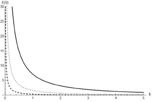
Figure 4 shows some plots of the expected failure time in the δ-shock model scenario. We note that E(S) is always decreasing as δ increases and, for fixed α  $(\beta)$, it takes larger (smaller) values for smaller values of β $(\alpha)$. $\mathbb{E}(S)$ (Eq. 38) with respect to δ for α = 1 with β = 0.5 (solid line), β = 1 (dotted line) and β = 2 (dashed line).
Conclusions
In the present manuscript, we analyzed three different classes of shock models governed by an inverse gamma mixed Poisson process. Generalizations of the Poisson process play a key role in modeling since, in many applied contexts, the assumption of exponentially distributed and independent interarrival times may be unrealistic. On the contrary, under the assumption of IGMP process, the interarrival times between shocks are dependent and represent a stationary series. The interarrival times follow the K-distribution which is characterized by heavy tails, this meaning that long interarrival times are observed with high probability. This property is shared by the Pòlya process, for which the interarrival times follow the Pareto distribution. However, the mean interarrival time of the Pòlya process can be infinite whereas the K-distribution has typically a finite mean. This property can be advantageous in applications where it is necessary to estimate or predict the average time between occurrences.
Shock models governed by IGMP processes are characterized by explicitly available finite dimensional distributions and free parameters allowing the model adaptation to a wide variety of data sets. For this reason they represent an alternative to shock models based on Pólya processes. Among the different classes of shock models we have analyzed: (i) the extreme shock model, (ii) the cumulative shock model and (iii) the δ-shock model and we have obtained the explicit expression of the survival function and the mean failure time. In particular, both in the extreme and cumulative shock models we prove that the system failure time is characterized by a decreasing failure rate. This property provides a crucial distinction of the IGMP shock model from other shock models characterized by an increasing failure rate. For instance, an extreme shock model with constant systems failure probability, under the assumption of shocks arriving according to a generalized Pólya process with constant baseline function, exhibits an increasing failure rate function.
In the proposed shock models certain independence assumptions could be weakened in order to describe more realistic scenarios. Indeed, in a future research, in order to show potential applications in engineering and actuarial sciences, we aim to study a cumulative shock model in which the damages Wk depend on the inter-arrivals Xk (see, for instance, Sumita and Shanthikumar [Reference Sumita and Shanthikumar37]). Moreover, other possible future researches involve (i) an extreme shock model when there are m possible sources of shocks acting on the system (see, for instance, Bozbulut and Eryilmaz [Reference Bozbulut and Eryilmaz6]) and (ii) a generalization of the cumulative shock model with a threshold R following a three parameter generalized exponential distribution (see Gupta and Kundu [Reference Gupta and Kundu22]).
Acknowledgments
The authors thank the anonymous referees for the useful comments that improved the paper.
Funding statement
This work is partially supported by MUR-PRIN 2022, project 2022XZSAFN “Anomalous Phenomena on Regular and Irregular Domains: Approximating Complexity for the Applied Sciences”, and MUR-PRIN 2022 PNRR, project P2022XSF5H “Stochastic Models in Biomathematics and Applications”, and by INdAM-GNCS, Project “Modelli di shock basati sul processo di conteggio geometrico e applicazioni alla soprav- vivenza”, CUP-E55F22000270001.
Competing interests
There were no competing interests to declare which arose during the preparation or publication process of this article.
Appendix A.
Appendix A.1. Fitting of real data
In this Appendix, we provide some examples of real data which can be appropriately described by the IGMP process. In particular, we consider two different datasets. The first one involves the occurrences of significant earthquakes registered in Italy from 1,961 to 2,018. The data have been collected by the National Geophysical Data Center of the U.S. Department of Commerce available at http://www.ngdc.noaa.gov/ngdc.html.
The second example concerns the number of hourly vessel arrivals at the Hong Kong Port throughout the month of May 2,014. The data have been collected from the website of the Maritime Department of Hong Kong and concern ocean-going vessels (see Huang [Reference Huang24]).
In both cases we perform a chi-square goodness of fit test in order to check if the data follow the distribution of the IGMP process or that of the Poisson process. We denote by  $\hat{N}(t)$ a Poisson process with parameter ϑ > 0, so that
 \begin{equation}
P(\hat{N}(t)=k)=\frac{(\vartheta t)^k}{k!} {\rm e}^{-\vartheta t} ,\quad \vartheta \gt 0, \quad k=0,1,2,\ldots.
\end{equation}
\begin{equation}
P(\hat{N}(t)=k)=\frac{(\vartheta t)^k}{k!} {\rm e}^{-\vartheta t} ,\quad \vartheta \gt 0, \quad k=0,1,2,\ldots.
\end{equation}  $\bullet$ A case study on seismology data
We provide the observed frequencies and compare them with the expected frequencies evaluated for (i) the IGMP process and (ii) the Poisson process. In all the cases, the parameters involved in the distribution are estimated by means of the Method of Moments and by using one year as the time unit. The critical value  $\chi^2_{0.05,n}$ is calculated at a significance level equal to 0.05 in the case of n degrees of freedom. The observations are classified into the mutually exclusive classes shown in Table A1 for the case (i) and in Table A2 for the case (ii).
Observed and expected frequencies of earthquakes in Italy for the IGMP process.

Observed and expected frequencies of earthquakes in Italy for the Poisson process.
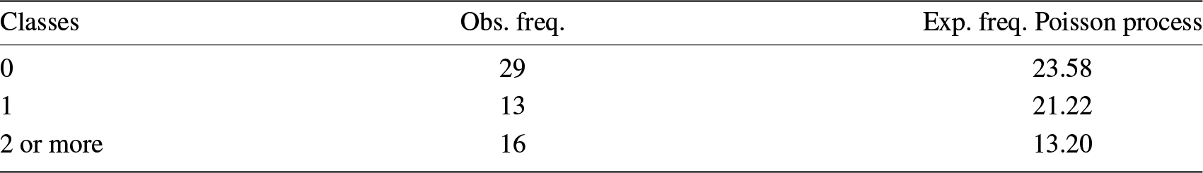
– Case (i): the estimated values of parameters of the IGMP process are α = 5.03 and β = 3.61. Since the χ 2-statistic takes value
$3.07 \lt \chi^2_{0.05,1}=3.84$, we cannot reject the null hypothesis of the distribution of the IGMP process.– Case (ii): the estimated value of the parameter of the Poisson distribution (A.1) is ϑ = 0.90. Hence, the χ 2-statistic takes value
$5.02 \gt \chi^2_{0.05,1}=3.84$ and we have to reject the null hypothesis of the distribution of the Poisson process.

 $\bullet$ A case study on vessel arrival data
As in the previous case, we carry out a chi-square test concerning (i) the IGMP process and (ii) the Poisson process. Since the dataset (cf. Table A1 of Huang [Reference Huang24]) counts how many times a fixed number of ships arrived within an hour, we set the time unit equal to one hour. The parameters in the distributions are estimated by the Method of Moments, and the critical value  $\chi^2_{0.05,n}$ is calculated at a significance level equal to 0.05 in the case of n degrees of freedom. The classes in which the data are divided, together with the observed and expected frequencies, are shown in Table A3.
– Case (i): the estimated values of parameters of the IGMP process are α = 14.8 and β = 41.38. Since the χ 2-statistic takes value
$5.5 \lt \chi^2_{0.05,6}=12.59$, we cannot reject the null hypothesis of the distribution of the IGMP process.– Case (ii): the estimated value of the parameter of the Poisson distribution (A.1) is ϑ = 2.99. The χ 2-statistic takes value
$16.61 \gt \chi^2_{0.05,7}=14.07$, so that we have to reject the null hypothesis of the distribution of the Poisson process.


Observed and expected frequencies of hourly vessel arrivals at the Hong Kong port for the IGMP process and for the Poisson process.

In Figure A1 we provide the empirical distribution function of the sample representing the vessel arrivals at the Hong Kong port, together with the theoretical cumulative distribution function of the IGMP process. The figure shows a large agreement between the empirical and the theoretical curve.
The empirical distribution function of the vessel arrivals’ sample (dotted line) compared with that of the IGMP process (solid line) cumulative distribution function.


 Open access