


1. Introduction
Sea ice algae are a fundamental source of primary production (PP) for polar zooplankton, particularly during the winter and early spring. In addition, there is growing evidence that sympagic production is likely critical for the health and survival of many polar fish, marine mammals and seabirds (Post and others, Reference Post2013). Brown and others (Reference Brown2018), for example, found in an analysis of the derived carbon in polar bear tissue that 72–100% was of sympagic origin, and in a Southern hemisphere study, Kohlbach and others (Reference Kohlbach2017) estimate that young and larval krill, a keystone species of the Southern Ocean trophic web, obtain up to 88% of their carbon budget from ice algae. Understanding the changing role of sea ice algal production through experimentation, observation and modeling will provide key insights into the ecological integrity and stability of polar regions. All these approaches have their challenges, and modeling is no exception. Yet incorporating sea ice algal dynamics in a global modeling context offers a promising tool for identifying and quantifying ocean, sea ice, land and atmosphere coupled constraints on sympagic PP.
This paper describes the polar biogeochemistry (BGC) of the Energy Exascale Earth System Model (E3SM) model version E3SMv1.1-BGC (Burrows and others, Reference Burrows2020). The model is designed for global climate applications and includes an active sea ice biogeochemical component (zbgc) with the goal of enhancing our understanding of the polar PP system. Here we contrast Arctic and Southern Ocean sea ice PP and biomass and identify the environmental conditions which contribute to these differences. We focus on the behavior of sea ice algae in fully-coupled Earth system simulations with active biogeochemical components in land, ocean and sea ice environments.
Sea ice forms seasonally from polar waters and as such, contains the bio-chemical signature of the ocean surface from which it forms. As ice crystals are unable to incorporate most alien molecules, salt retained during initial formation is concentrated in fluid pockets and channels creating a multiphase and protected habitat for microscopic organisms and algae (Krembs and others, Reference Krembs, Gradinger and Spindler2000). Ice algae can be found throughout the sea ice interior, though observations indicate regional patterns in vertical distribution. Arctic sea ice algae favor the bottom 3–5 cm of the ice (Lee and others, Reference Lee, Whitledge and Kang2008; Cota and others, Reference Cota, Legendre, Gosselin and Ingram1991; Gradinger and others, Reference Gradinger, Iken and Bluhm2012; Michel and others, Reference Michel, Nielsen, Nozais and Gosselin2002), while Southern Ocean ice algae also thrive in freeboard and internal ice communities (Ackley and Sullivan, Reference Ackley and Sullivan1994; Meiners, Reference Meiners2013). These polar and regional differences are believed to derive from the sea ice physical micro- and macro-scale seasonal dynamics (Fritsen and others, Reference Fritsen, Lytle, Ackley and Sullivan1994). For example, the gradual expulsion of salt through gravity drainage – convective overturning of unstably stratified brine – serves as a resupply mechanism for nutrients, exchanging internal, depleted brine concentrations with the underlying ocean reservoir (Cox and Weeks, Reference Cox and Weeks1975; Weeks and Ackley, Reference Weeks and Ackley1986). Conversely, very cold temperatures and low salinities reduce sea ice permeability, constricting brine passages and isolating organisms from interior layers (Ackley and Sullivan, Reference Ackley and Sullivan1994; Vancoppenolle and others, Reference Vancoppenolle, Bitz and Fichefet2007, Reference Vancoppenolle, Fichefet and Bitz2005). At still other times for warmer ice, pressure forces from snow and melt water induce internal brine flow which may flood the snow with nutrient-rich brine, or flush the interior ice with low salinity melt water (Ackley and Sullivan, Reference Ackley and Sullivan1994; Eicken and others, Reference Eicken, Krouse, Kadko and Perovich2002). The former process, snow loading and flooding, is believed to be key to the development of the freeboard algal communities of the Southern Ocean (Ackley and others, Reference Ackley, Lewis, Fritsen and Xie2008) while the latter process, melt water flushing, plays a role in the timing of sea ice chlorophyll-a (chl-a) decline and release to ocean waters.
The eight-component sea ice biogeochemical model (zbgc) presented in this work is designed to capture some of the above physical processes that control the vertical distribution of ice algae. The model is resolved in three spatial dimensions with resolution on the order of centimeters. The simulations presented here use eight vertical grid layers to minimize computational cost. We found a three fold increase in compute time for stand-alone sea ice simulations when using the eight grid layer version described here over a skeletal layer sea ice biogeochemical model. Vertical transport of biogeochemical tracers is controlled by internal brine dynamics which evolve according to a mushy layer halodynamics algorithm (Turner and Hunke, Reference Turner and Hunke2015). This algorithm includes flushing and gravity drainage parameterizations. The zbgc module includes adsorption and desorption at the ice crystal/brine interfaces for algae and various chemical species, such as dissolved iron and ammonium. In addition, a simple parameterization of ice diatom motility is included which allows diatoms to maintain their relative vertical position in the ice for low melt rates.
In this study, we analyze results from 157 years of historical simulation and a parallel run with constant 1850 atmospheric forcing, using the fully coupled E3SMv1.1 model. Our analysis focuses on sea ice and upper ocean properties that exert important controls on sea ice algal chl-a and PP. Here we find some significant biases in both simulations that directly impact sea ice PP: specifically, regional biases in sea ice volume and extent, as well as biases in upper ocean physical and biogeochemical properties.
This paper is organized as follows. In the first sections, we provide a general description of the E3SMv1.1-BGC configuration, MPAS-O BGC (Model for Prediction Across Scales – Ocean Biogeochemistry) and simulations used in the analysis. Further details on the E3SMv1.0 model and the E3SMv1.1 biogeochemical configuration can be found in Golaz and others (Reference Golaz2019) and Burrows and others (Reference Burrows2020), respectively. We continue with a detailed description of MPAS-Seaice physical and biogeochemical routines and tuning approach. Analysis of simulated results begins with a comparison of pre-industrial and historical simulations. We compare simulated sea ice chl-a with observations. We then focus on the 157-year constant-forcing simulation, analyze the ocean and sea ice state and suggest controls on net sea ice PP in the Arctic and Southern Ocean. For this analysis we define and map bounds for maximal sea ice algal growth from both observations and model output to better understand the constraints on ice algal production. We then consider temporal variability in the sea ice algal production and chl-a biomass. Discussion and conclusions follow.
2. E3SM v1 coupled BGC configuration
Results analyzed in this work are primarily from a 157-year control simulation (CNST-forcing) of the fully coupled E3SMv1.1 model with active BGC in the ocean, sea ice and land models (Burrows and others, Reference Burrows2020). In this simulation, atmospheric concentrations of greenhouse gases and aerosols are fixed at 1850 conditions. We also compare results with the last 20 years (1990–2009) of an historically forced simulation (HIST-forcing). In this run, atmospheric greenhouse gases and aerosols follow prescribed historical pathways (described in Golaz and others. (2019, Appendix B) following the input4MIPS datasets). E3SMv1.1 uses the base resolution of 110-km grid spacing for the atmosphere and land components; 60-km grid spacing in the midlatitudes to 30-km spacing in the equatorial and polar regions in the ocean and sea ice; and 55-km grid spacing in the river transport model.
E3SMv1.1 ocean and sea ice BGC are responsive to climate conditions but do not feed back on the physical system. Both models are newly implemented in the MPAS unstructured grid framework which uses non-uniform polygon meshes. These simulations represent the first investigation of global sea ice PP in the E3SM model with sea ice–ocean biogeochemical coupling.
The ocean biogeochemical component is adapted from the Biogeochemical Elemental Cycling (BEC) model (Moore and others, Reference Moore, Doney, Kleypas, Glover and Fung2001; Moore and others, Reference Moore, Doney and Lindsay2004) with modifications to allow implementation in the MPAS-O (Ringler and others, Reference Ringler2013) unstructured grid framework and two-way coupling with sea ice biogeochemical tracers. A description of the ecosystem components and behavior is given in Moore and others (Reference Moore, Doney and Lindsay2004). The E3SMv1.1 version also includes explicit representation of the Prymnesiophyte, Phaeocystis sp. developed by Wang and others (Reference Wang, Elliott, Maltrud and Cameron-Smith2015).
2.1. MPAS-Seaice zbgc
The MPAS-Seaice model evolves a set of physical ice variables (including enthalpy, salinity, ice concentration, ice and snow volume, and melt pond volume and area) which characterize the sea ice state and enable assessment of coupled interactions with other Earth system components. Version 1.0 is adapted from CICE (the Los Alamos sea ice model; Hunke and other (Reference Hunke, Lipscomb, Turner, Jeffery and Elliott2013) and Hunke and Dukowicz (Reference Hunke and Dukowicz2002)) for non-regular polygons (Golaz and others, Reference Golaz2019) and implemented on a B-grid with state scalars (sea ice concentration, temperature, salinity and biogeochemical tracers) on cell centers and velocity components defined on cell vertices. MPAS-Seaice uses the Icepack library, version 1.0.2 (Hunke and others, Reference Hunke2018) for its column physics and BGC.
The sea ice physics package and dynamical core is comprised of several submodules representing the following key sea ice processes: (1) mushy layer thermodynamics (with temperature and salinity evolution from Turner and others (Reference Turner, Hunke and Bitz2013)), which defines sea ice and snow growth and melt due to conductive, radiative, salinity and turbulent fluxes; (2) shortwave radiative transfer using the delta-Eddington multiple-scattering scheme of Briegleb and Light (Reference Briegleb and Light2007); (3) sea ice momentum which evolves the ice velocity field assuming an elastic-viscous-plastic rheology (Hunke and Dukowicz, Reference Hunke and Dukowicz1997); (4) incremental remapping transport which describes advection of ice concentration, volume, physical and biogeochemical tracers, and other state variables (Lipscomb and Hunke, Reference Lipscomb and Hunke2004); and (5) a ridging parameterization which transfers sea ice concentration between each of the five sub-grid thickness categories (Lipscomb and others, Reference Lipscomb, Hunke, Maslowski and Jakacki2007).
The zbgc (vertically resolved, biogeochemical) submodule uses information about the sea ice state, particularly the vertical distribution of temperature, salinity and internal shortwave radiation, and changes to the ice and snow thicknesses, to determine vertical boundary flux velocities and internal changes in brine tracer concentrations from sea ice physics processes. Biogeochemical exchanges are modeled as coupled non-linear reaction terms (Appendix: Biogeochemical Reaction Terms).
The zbgc submodule procedure is as follows. At each time step and in each of five thickness categories within a given horizontal grid cell, solve mushy layer thermodynamics to update vertical profiles of ice/snow enthalpy and salinity and compute thermodynamic changes in the ice/snow thicknesses. Next, compute microstructural characteristics (porosity, permeability, gravity drainage diffusivity, Darcy flow velocities) from the ice temperature and salinity profiles and ice boundary growth and melt rates after (Jeffery and others, Reference Jeffery, Hunke and Elliott2011). Use this information to solve for the change in brine level (Appendix: Brine Evolution) relative to the sea ice surface. Then determine the mobile and attached fractions for each biogeochemical tracer (section: Mobile and attached tracers) and solve the vertical transport equation for the mobile tracers (section: zbgc tracer equation) and melt losses of attached tracers. Finally, compute the coupled set of non-linear biogeochemical reaction terms for each brine tracer concentration (Appendix: Biogeochemical Reaction Terms). The remaining sea ice redistribution and horizontal transport processes are then performed while conserving the total brine volume of each biogeochemical tracer. The five sets of biogeochemical variables, one for each subgrid thickness category, are retained at each time step and saved as output data. All the results presented in this work are from the net horizontal grid cell tracer field computed as a category sum weighted by sea ice area concentration.
2.2. The sea ice algal ecosystem
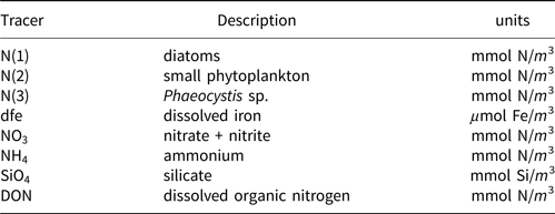
The zbgc model configuration used in this analysis has eight components (see Table 1 for symbols used in this text): three algal groups measured in units of nitrogen (diatoms, small plankton and Phaeocystis sp.), three macro-nutrients (nitrate + nitrite, silicate and ammonium), one micro-nutrient (dissolved iron) and dissolved organic nitrogen. We assume that phosphorus is generally not a limiting macro-nutrient in the sea ice (Deal and others, Reference Deal2011. This is consistent with the findings of Saenz and Arrigo (Reference Saenz and Arrigo2012) for Southern Ocean sea ice. However, we acknowledge observational evidence which suggests potential phosphorus limitation of sea ice algae in the Baltic Sea (Piiparinen and others, Reference Piiparinen, Kuosa and Rintala2010). Conversions to carbon, silica and iron are based on fixed prescribed ratios. All components are two-way coupled with MPAS-O BGC. A schematic of zbgc and biogeochemical interactions with the ocean are depicted in Figure 1. Our choice of ecosystem components is based on Deal and others (Reference Deal2011), which includes only the dominant biogeochemical controls on total sea ice algal chl-a: sea ice diatoms, nitrate, ammonium and silicate. In this study, we expand to eight fields to allow for potentially interesting interactions with the polar marine PP system. For example, though ice diatoms tend to dominate sea ice chl-a observations, we also include the prymnesiophyte, Phaeocystis sp. and small flagellates which can be present in abundance (Lizotte, Reference Lizotte2015), contribute significant fractions to the polar oceanic system and are important producers of dimethyl sulfide. In addition, though sea ice algae are generally not observed to be iron-limited (Lannuzel and others, Reference Lannuzel2016), we include dissolved iron in our component fields because sea ice melt is thought to be an important source of the micro-nutrient for Southern Ocean phytoplankton (Lannuzel and others, Reference Lannuzel2013). Finally, dissolved organic nitrogen is included in sea ice to track production and exchange with the ocean. This feature is essentially diagnostic with respect to sea ice production, though in future versions we plan to add sympagic remineralization.
Schematic of coupled components in the E3SMv1.1 sea ice–ocean eco-dynamics. Boxes represent biogeochemical fields. Thin arrows are fluxes between components. Thick arrows between ice algal/phytoplankton groups indicate fluxes involving the entire group while the thin arrow represents a flux between silicate and diatoms. The thick open arrow indicates respective fluxes: ice diatoms exchange with ocean diatoms, small flagellates with small phytoplankton, and Phaeocystis sp. with its ocean counterpart. Only shown are ocean biogeochemical components involved in direct fluxes with the sea ice. MPAS-O BGC also includes inorganic carbonate chemistry, phosphate, zooplankton, sinking detrital pools, diazotrophs and coccolithophores assigned as implicit members of the small plankton group.

Sea ice biogeochemical tracers
2.3. Mobile and attached tracers
One basic assumption of our ice biogeochemical model is that BGC tracers are only present in the sea ice brine. Consequently, the vertical domain for the zbgc model consists of only brine saturated sea ice. We do not, however, require that all sea ice have non-zero brine volume or that the brine surface level within the ice crystal matrix equal the ice surface. For Arctic sea ice under light snow conditions, the ice surface typically rises above the ocean surface, draining the upper ice of brine. The resulting equilibrium brine level then lies below the upper $\sim 10\percnt$ of the ice. By contrast, in many regions of the Southern Ocean, relatively heavy snow depresses the ice below the ocean surface, driving brine intrusions into the snow layer. In this case, the brine level lies above the ice surface, and so does the vertical extent of the zbgc model. Motion of the brine level (h b) is fundamentally a result of gravitational forces and depends on the permeability of the ice, changes in the ice bottom and surface boundaries, and surface sources of water: snow and ice meltwater, sea water flooding and liquid precipitation. A full description of the brine level dynamics equation is given in the Appendix: Brine Evolution.
The extent to which bio-chemical tracers are advected by the brine depends upon whether the tracer is dissolved or particulate and whether it has some affinity for the ice crystal/fluid boundary. Ice algal diatoms are well known for their ability to attach to ice crystals by means of frustules. In addition, sea ice algae produce ice-active proteins in exopolysaccharids that potentially increase ice affinity (Boetius and others, Reference Boetius, Anesio, Deming, Mikucki and Rapp2015; Juhl and others, Reference Juhl, Krembs and Meiners2011). Indeed, ice diatoms not only resist brine motion through attachment, but actively migrate within the ice domain. Early estimates suggest diatoms move at speeds of 1.5 cm/d (Welch and Bergmann, Reference Welch and Bergmann1989), while more recent lab studies found speeds of 14.4 cm/d (Aumack and others, Reference Aumack, Juhl and Krembs2014; Krembs and others, Reference Krembs, Gradinger and Spindler2000).
In contrast, the dissolved salts, nitrate and silicate, are treated as purely mobile (Fripiat and others, Reference Fripiat2014) and their transport strongly governed by brine motion. This may be an oversimplification, however, as there is some evidence of enhanced nitrate levels in sea ice in the Norwegian Young sea ICE cruise (N-ICE2015; (Duarte and others, Reference Duarte2017; Fripiat and others, Reference Fripiat, Sigman, Massé and Tison2015)). Still, there is more definitive evidence that ammonium and organic matter produced by phytoplankton have an affinity for the ice matrix (Fripiat and others, Reference Fripiat2014; Müller and others, Reference Müller2013; Verdugo and others, Reference Verdugo2004). This is likely due to the prevalence of colloidal matter including nano- and microgels which adhere to the ice crystals. Similarly, Lannuzel and others (Reference Lannuzel2016) report that dissolved iron is actively extracted from ocean water during sea ice growth and incorporated into the sea ice matrix through adsorption onto particles such as organic ligands.
In general, we assume that the brine concentration of bio-chemical tracers may be present in both a purely mobile phase, c m, which advects with the brine, and an attached (or stationary) phase, c s, which adheres to the ice crystals or adsorbing particles. Algal diatom locomotion is treated separately and discussed below. The mobility of small flagellates is assumed to be ineffective against ice melt losses. Transfer between phases is governed by prescribed adsorption/desorption timescales and the assumption that ice growth enables adsorption while ice melt facilitates desorption.
Our treatment is based on the linear adsorption model of Harmand and others (Reference Harmand, Rodier, Sardin and Dodds1996). Sea ice biogeochemical tracers adhere to ice crystals with a time constant of τret, and release with a time constant τrel, i.e.

where c m is the mobile phase tracer concentration and c s is the attached phase concentration. The time constants are modeled as crude functions of the ice growth and melt rates defined as changes in the ice thickness (dh/dt). All tracers except algal diatoms follow the simple rule: when dh/dt ≥ 0, then τ rel → ∞ and τ ret is finite. For dh/dt < 0, then τ ret → ∞ and τ rel is finite. In this way, ice growth promotes adsorption while ice melt enables transitions to the mobile phase. Currently, there is a lack of observational and experimental data to motivate a more sophisticated parameterization. Even with this approach, there are potentially 2N additional unknown parameters representing the adsorption/desorption time constants for an N component biochemical ecosystem. To alleviate the proliferation of unconstrained model parameters, we assume all multi-phase tracers adsorb/desorb in the same manner and specify only two time constants.
The adsorption of tracers is also bound by a saturation concentration which is determined from geometric properties of the ice crystals and adsorbing particles (assumed to be spheres). Johnson and others (Reference Johnson, Blue, Logan and Arnold1995) define the maximum number of adsorbate that can attach to a given collector during porous transport, S d:
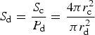
where S c is the surface area of the collector crystal and P d is the projected area of the adsorbate (e.g. diatom). For sea ice diatom attachment to ice crystals, we use a diatom radius of r d = 4.7 μm corresponding to a cell volume of 435 μm3, which is appropriate for Nitzschia frigida (Olenina and others, Reference Olenina2006), and an ice crystal radius of r c = 3000 μm (Weeks, Reference Weeks2010). This is then multiplied by the ice crystal number density times the fraction of diatom surface area available for attachment (Johnson and others, Reference Johnson, Blue, Logan and Arnold1995). We calculate the ice crystal number density for each vertical layer as $\lpar 1-\phi \rpar \delta h\pi r_{\rm c}^2/V_{\rm c}$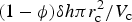 , where V c is the ice crystal volume assumed to be spherical, δh is the ice thickness in a vertical grid layer, and $\delta h \pi r_{\rm c}^2$
 is the volume of an ice layer column of radius r c. When the stationary concentration reaches the saturation concentration, adsorption stops and the additional material remains in the mobile phase.
Diatoms are distinct from other tracers in that they can move independently. Although we do not model motility as an advective mechanism, we assume that diatoms actively maintain their relative position within the ice, i.e. bottom (interior, upper) algae remain in the bottom (interior, upper) ice, unless melt rates exceed a threshold, v algae. See Table 2 for parameter values.
MPAS-Seaice zbgc reaction parameters
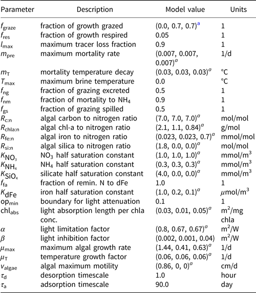
a Parameters for 1) diatoms, 2) small flagellates and 3) Phaeocystis sp., respectively
2.4. zbgc tracer equation
Purely mobile biogeochemical tracers are tracers which move with the brine and thus, in the absence of biochemical reactions, are transported like salinity. The flux-conserved quantity for purely mobile tracers is the column integrated bulk tracer concentration in the ice column, i.e. C = h bϕ[c], where h b is the brine level, ϕ is the porosity and [c] is the in situ brine tracer concentration.
The continuity equation is (Jeffery and others, Reference Jeffery, Hunke and Elliott2011 Eq. (A3)):

where w is the Darcy velocity (A3), D = D MLD + ϕD m is a combination of the effective molecular diffusivity (D m) scaled by the porosity and the mixing length diffusivity (D MLD of Jeffery and others (Reference Jeffery, Hunke and Elliott2011)), and R([c]1, [c]2, …[c]N) are biogeochemical reaction terms described in detail in Appendix: Biogeochemical Reaction Terms. In general, the biogeochemical reaction terms are non-linear functions of the N ecosystem tracer brine concentrations.
The vertical coordinate, Z ∈ [Z bot(t), Z top(t)], defines a domain bounded by the ice bottom and brine level surface, and so (3) represents a moving boundary problem. The biogeochemical module solves this equation on a fixed domain z ∈ [0, 1] through the coordinate transformation z = (Z top − Z)/(Z top − Z bot). The resulting equation (Jeffery and others, Reference Jeffery, Hunke and Elliott2011 eqn (C16)):
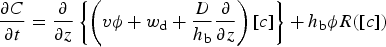
includes an additional advection term v:
which explicitly accounts for changes in the sea ice thickness from melt and ice growth.
Solutions to (4) are found using a flux-corrected and positive definite finite element Gelerkin discretization (Brenner and Scott, Reference Brenner and Scott2005; Jeffery and others, Reference Jeffery, Elliott, Hunke and Lipscomb2016).
2.5. Tuning and model parameters
MPAS-Seaice zbgc is part of ICEPACK, the CICE/Consortium column package (Hunke and others, Reference Hunke2018). Parameter values were first tuned in 1-D sea ice only configurations of the Arctic (N-ICE2015 forcing data set; Duarte and others, Reference Duarte2017), and initial tuning of the tracer transport physics was conducted using the Southern Ocean ISPOL forcing data set (Jeffery and Hunke, Reference Jeffery and Hunke2014). Parameters were adjusted using the fully coupled simulations in the HiLAT-E3SM.v0 configuration (Hecht and others, Reference Hecht2019) and tested over 10-year periods during ~200 years of ocean–sea ice spin-up of E3SMv1.1. In all 3-D model configurations, the primary tuning criterion was agreement between observations and simulated ice-integrated chl-a using field measurements from six locations: three in the Arctic (N-ICE2015 (Duarte and others, Reference Duarte2017); Point Barrow (Lee and others, Reference Lee, Whitledge and Kang2008); and BEST (Gradinger and others, Reference Gradinger, Iken and Bluhm2012)) and three in the Southern Ocean (ISPOL (Lannuzel and others, Reference Lannuzel2013); Marguerite Bay (Massom and others, Reference Massom2006); Prydz Bay (Laybourn-Parry, Reference Laybourn-Parry2012)).
For simplicity and to reduce the number of tunable parameters, this version of the model assumes that new sources of nitrogen to the sea ice (primarily nitrate, though there is a small ammonium flux from the ocean) dominate sea ice PP. In other words, in situ remineralized nitrogen is restricted to ammonium sources from the grazing of algae and their natural mortality, and not remineralization of the dissolved organic nitrogen pool, which is difficult to validate. As a further simplification, nitrification rates are set to zero.
As previously discussed, nitrate and silicate are treated as purely mobile tracers. All other tracers attach with an hour timescale and release on a 90-day timescale. Long release timescales allow for high retention of biomass throughout the spring, resisting melt-water flushing of biogeochemical material. Short adsorption timescales allow for maximal seeding of the initial population during sea ice formation and minimize loss of newly produced algal biomass from brine exchange with the ocean. Given that the time-step for MPAS-Seaice is 30 min, 1 h represents a near lower bound for the attachment timescale. Loss of ice mass, however, removes both attached and mobile tracers. The exceptions are the diatoms, the primary algal group, which actively migrate in the sea ice to retain their relative position with respect to the ice bottom. We use a moderate rate of 0.86 cm/d, which is half the rate assumed by Lavoie and others (Reference Lavoie, Denman and Michel2005) and well within the observed migration rates (Welch and Bergmann, Reference Welch and Bergmann1989; Aumack and others, Reference Aumack, Juhl and Krembs2014; Krembs and others, Reference Krembs, Gradinger and Spindler2000).
The three algal groups are distinguished in the following ways. Ice diatoms are the only group with a demand for silica. We use a silicate uptake half-saturation constant of 4 mmol/m3 (Lavoie and others, Reference Lavoie, Denman and Michel2005). The algal growth parameters follow Jin and others (Reference Jin2006) for diatoms: maximum specific algal growth rates of 1.44 1/d, light limitation factor of 0.8 m2/d and light inhibition factor of 0.002 m2/d. For estimates of prymnesiophyte growth parameters, Arrigo and others (Reference Arrigo, Mock and Lizotte2010) report maximum specific growth rates of 0.35–0.71 1/d for P. antarctica, which grows well in Southern Ocean sea ice and open ocean. We use the intermediate value of 0.63 1/d and a light inhibition factor of 0.04 m2/W. There are insufficient observations to constrain growth parameters for the small flagellate group. However, we assume a distinct niche from the other algal groups by specifying the lowest maximum specific growth rate (0.41 1/d) but relatively weak light inhibition (0.001 m2/W). We also assume that small plankton and Phaeocystis sp. experience higher grazing pressure as observed in pelagic phytoplankton communities (Yang and others, Reference Yang, Ha and Kang2015) in addition to mortality, while ice diatoms losses occur through mortality alone. This assumption produces ice algal assemblages dominated by diatoms in both poles (Lizotte, Reference Lizotte2015; Arrigo and others, Reference Arrigo, Worthen, Lizotte, Dixon and Dieckmann1997; Arrigo, Reference Arrigo2003).
The most important tuning parameters are predation rate (fgraze), modeled as a fraction of production; mortality rate (mpre); the mixing length parameter (l sk) which governs the strength of gravity drainage fluxes for biogeochemical tracers; and adsorption/retention timescales. Table 2 lists biogeochemical reaction parameters and chosen values. During the tuning process, we found that modeled sea ice algal chl-a tended to be biased low, particularly in the Arctic. As a result, our chosen parameter values skew toward (1) maximizing algal access to ocean nutrients (i.e. high gravity drainage fluxes; l sk = 20 m), (2) enhancing chl-a retention in the sea ice (short adsorption and long retention timescales) and (3) reducing predation and mortality of algal groups. We understand now that biases in the climate state (discussed further in Simulation results and Discussion) contribute significantly to these underestimations.
3. Simulation results
Burrows and others (Reference Burrows2020) present a detailed overview of the E3SMv1.1-BGC pre-industrial control (CNST-forcing) and historical (HIST-forcing; or BDRD-hist in Burrows and others (Reference Burrows2020)) simulations with an emphasis on interactions between land nitrogen and phosphorous nutrient cycles and the global carbon-climate feedbacks. Here we confine our analysis to the Arctic and Southern Oceans and consider how spatial and temporal variability in the polar climate state influence sea ice algal chl-a biomass and PP. We restrict our analysis to total chl-a and net PP fields, that is, the summed contribution of all three algal groups. In addition, all simulation analysis is derived from monthly mean fields. For sea ice variables, presented results are averages over the five sub-grid thickness categories.
3.1. HIST-forcing and CNST-forcing
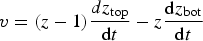
For the majority of our analysis, we use the CNST-forcing simulation because it represents a relatively stable 157-year time-series of natural system variability. The HIST-forcing simulation, though more representative of the atmospheric forcing conditions on Earth in the last 40 years of the simulation, has a too strong aerosol-cloud effect in response to industrial aerosol emissions which produces enhanced initial cooling of the Arctic (also observed in the E3SMv1.0-DECK simulations of Golaz and others (Reference Golaz2019)). The result is sharp increases in Arctic sea ice volume and extent relative to CNST-forcing beginning in the early 1970s. Figure 2 shows five-year running means of integrated sea ice area and volume for both simulations. Decreasing trends in Arctic ice area and volume in HIST-forcing begin in the mid to late 1970s with values returning to pre-industrial levels over the final 20 years of simulation. Simulated Arctic sea ice area exceeds mean observations (Cavalieri and others, Reference Cavalieri, Parkinson, Gloersen and Zwally1996) by ~1 million km2 for CNST-forcing, and between 0.5 and 3 million km2 for HIST-forcing. The additional sea ice is primarily an artificial extension in the Labrador Sea likely due to insufficient resolution in ocean circulation around the southern tip of Greenland (Burrows and others, Reference Burrows2020). Southern Ocean sea ice area is more consistent with SSMI observations (Cavalieri and others, Reference Cavalieri, Parkinson, Gloersen and Zwally1996) particularly for HIST-forcing over the final 30 years. Unlike the Arctic, industrial aerosol concentrations do not play a significant role in Southern Ocean ice extent or volume. Extent and volume trends in HIST-forcing are weaker but notably decreasing from the early 1980s. Over the final 30 years, Southern Ocean CNST-forcing extent exceeds HIST-forcing by ~1.2 million km2.
Five-year running means of hemispheric integrated (a,b) sea ice area (million km2), (c,d) sea ice volume (1000 km3) and (e,f) net sea ice algal primary production (PP, TgC/a) for CNST-forcing (blue) and HIST-forcing (red) simulations. Northern hemisphere averages are shown in the left column while Southern hemisphere are on the right. Only grid cells with at least 15% sea ice concentration are included in the averaging. Also shown is the 1979–present mean sea ice area (black dashed line, (Cavalieri and others, Reference Cavalieri, Parkinson, Gloersen and Zwally1996)) and PIOMAS estimate of Arctic sea ice volume (black solid line, (Schweiger and others, Reference Schweiger2011)).
Mean annual sea ice PP in the Arctic is on the low side of previous estimates even with too extensive mean sea ice. This suggests that both HIST-forcing and CNST-forcing likely underestimate per area PP rates. HIST-forcing mean values fluctuate between ~5.8 and 9 TgC/a while CNST-forcing has generally lower values ranging between 5 and 7 TgC/a. Previous field estimates vary by an order of magnitude with 6 TgC/a (Subba-Rau and Platt, Reference Subba-Rau and Platt1984) and from 9 to 73 TgC/a (Legendre and others, Reference Legendre1992). Modeling studies estimate 10.1 TgC/a (Deal and others, Reference Deal2011) to 36 TgC/a (Dupont, Reference Dupont2012). Increases in primary production in HIST-forcing relative to CNST-forcing occur during the years of high Arctic sea ice area in the 1970s and 1980s. However, we also see slightly higher net sea ice PP per ice area in the last 30 years of HIST-forcing (570–650 mgC/m2/a) relative to CNST-forcing (500–610 mgC/m2/a). This suggests that the regions in HIST-forcing of more extensive sea ice are also regions of greater sea ice primary production density.
Five-year running mean values of Southern Ocean sea ice primary production range between 11 and 20 TgC/a. These values are again low compared to previous estimates from field observations 63–70 TgC/a (Legendre and others, Reference Legendre1992) though more consistent with the range in model estimates: 23.7 (Saenz and Arrigo, Reference Saenz and Arrigo2014) to 35.7 TgC/a (Arrigo and others, Reference Arrigo, Worthen, Lizotte, Dixon and Dieckmann1997). CNST-forcing and HIST-forcing estimates are similar, and differences generally reflect variability in sea ice area. Average PP per ice area is similar in both simulations, ranging from 1400 to 1700 mgC/m2/a.
Sea ice PP observations are relatively scarce and not sufficient for ice algal model validation on a global scale. Rather, sea ice core measurements of algal chl-a offer the most extensive comparison. Figures 3 and 4 show seasonal cycles of column integrated sea ice algal chl-a from HIST-forcing and CNST-forcing simulations at several locations in the Arctic and Southern Ocean, respectively, contrasted with core measurements. The shaded regions in the Arctic figure indicate the range in simulated monthly mean over the 157-year CNST-forcing time-series and the final 20 years of HIST-forcing. Individual cores are indicated as well as observational monthly means and standard deviations. For the Arctic, core observations are from (a) the Bering Sea (Gradinger and others, Reference Gradinger, Iken and Bluhm2012), (b) Baffin Bay (Michel and others, Reference Michel, Nielsen, Nozais and Gosselin2002), (c) the Norwegian Sea (Duarte and others, Reference Duarte2017), (d) Point Barrow (Lee and others, Reference Lee, Whitledge and Kang2008 and C. Deal, pers. comm.), (e) the Lincoln Sea (Lange and others, Reference Lange2015), (f) the Canadian Arctic (Melnikov and others, Reference Melnikov, Kolosova, Welch and Zhitina2002) and (g,h) the Beaufort Sea (Horner and Schrader, Reference Horner and Schrader1982; Alou-Font and others, Reference Alou-Font, Mundy, Roy, Gosselin and Agusti2013, respectively). Simulated chl-a is most consistent with observations in the Bering Sea and Point Barrow, which is perhaps not surprising given that both these locations were used in model tuning. Modeled chl-a is within the range of observations in the Baffin Bay and Beaufort Seas, though with some discrepancies in the seasonal cycle. In the Norwegian Sea, model results suggest values as high as 10 mg/m2, nearly an order of magnitude larger than observations. However, the reported measurements were taken from a newly formed lead and perhaps do not generally represent sea ice in this region (Duarte and others, Reference Duarte2017). In the Lincoln Sea and Canadian Arctic, the model overpredicts chl-a concentrations, though by only 1–3 mg/m2. This is because observations in these locations indicate very low chl-a (< 3 mg/m2). In fact, the peak in observations is more consistent with the modeled minima. Notably, for the Canadian Arctic, the change in chl-a over the seasonal cycle is similar to observations. This may indicate that modeled losses of algae in the spring and summer are too weak. We note here that low simulated primary production is potentially incongruous with reasonably well simulated chl-a. We discuss the implications of this result in detail in the Discussion section.
Monthly simulated sea ice algal chlorophyll-a concentrations (mg/m2) in CNST-forcing (blue; averaged over 157 years) and HIST-forcing (red; averaged over the last 20 years) plotted against year day for eight locations (a–h) in the Arctic. Shaded regions indicate the range in monthly means. Also shown are core observations: both individual measurements (open circles) and monthly means (solid diamonds with ±1 std). Data references are in text.

Monthly simulated sea ice algal chlorophyll-a concentrations (mg/m2) in CNST-forcing (blue line; averaged over 157 years) and HIST-forcing (red line; averaged over the last 20 years) plotted against day of year for all grid points in six regions (a–f) (as defined in Meiners and others (Reference Meiners2012)). Shaded regions represent the range in the monthly mean. Also shown are time-series averages of the CNST-forcing monthly mean chlorophyll-a computed at grid cells corresponding to observed core locations for each region (light blue squares with 1 std error bars). Core observations are depicted as black symbols; both individual core measurements (open circles) and monthly means (solid diamonds with ± 1 std) are shown. Data references are in text.

The Southern Ocean observations (Fig. 4) are from the ASPECT data set (Meiners, Reference Meiners2013) and represent a compilation of field campaigns. The red (HIST-forcing) and blue (CNST-forcing) curves and shaded regions are averages over all grid cells in six regions defined as sectors south of 50°S and bounded by the following latitudinal lines (Meiners and others, Reference Meiners2012): (a) the Western Weddell (300 to 315°E), (b) Eastern Weddell (− 45 to 20°E), (c) Indian Sector (20 to90°E), (d) Pacific Sector (90 to 160°E), (e) Ross Sea (160 to 230°E) and (f) Bellingshausen/Amundsen Seas (230 to 300°E). The shaded regions are the range in monthly means over the time-series. Also shown in light blue symbols with 1 std error bars is the monthly mean CNST-forcing climatology, using only grid cells corresponding to core measurement locations for each region. In general, the two simulations are quite similar. In addition, simulated mean climatology generated from grid cells at core locations is consistent with that using all grid points except perhaps in the Indian Sector, where temporal coverage of observations is sparse. Agreement between model and observations is better in the Southern Ocean than the Arctic, though admittedly averaging over a wider spatial region smooths over heterogeneity in the data. Notably, simulated climatology from grid cells at core locations (light blue squares) is not more consistent with observations than the regional average except for perhaps during a couple months of the year in the Pacific Sector and Western/Eastern Weddell. Overall, modeled monthly mean Southern Ocean chl-a is somewhat overestimated except perhaps in the Bellingshausen/Amundsen sector.
With respect to the modeled pre-industrial and historical time periods, differences in sea ice chl-a at observed locations and sectors are smaller than differences between simulations and observations. Several locations show possible increases in peak biomass over the last 20 years of HIST-forcing compared to pre-industrial: the Norwegian and Lincoln Seas, Baffin Bay, the Beaufort and perhaps the Pacific Sector, Ross Sea and Bellingshausen/Amundsen sectors. However, all increases are well within the range of CNST-forcing monthly means (Figs. 3 and 4). For this reason, we focus the remainder of our analysis on the CNST-forcing simulation with the understanding that the primary discrepancies between model and observations are likely not due to the transient forcing conditions of the industrial historical period.
3.2. Ocean and sea ice state
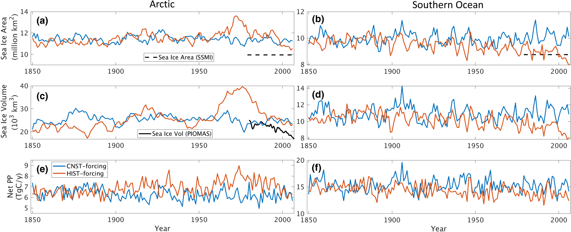
Based on the results from the previous section, the E3SMv1.1 model simulates low values of net annual sea ice PP in both polar regions. In order to understand the processes behind these values, it is critical to first assess the quality of the modeled polar climate state as it pertains to the sea ice algal ecosystem. Figures 5 and 6 show contours of the mean surface ocean nutrients, nitrate and silicate, respectively, in the Arctic and Southern Oceans. The upper row depicts seasonal means in Arctic winter/austral summer (JFM, January–March) and summer/austral winter (JAS, July–September). Figure 5a is notable for the low values in surface nitrate during winter and early spring, particularly in the Chukchi and Canadian Arctic waters. The second row are differences between World Ocean Atlas observations (Garcia and others, Reference Garcia2009) and modeled values. The large regions of red shading in winter and summer in both figures and in both poles indicate systemic underestimations in modeled surface ocean macro-nutrients.
Upper row are mean surface ocean nitrate concentrations (mmol/m3) in CNST-forcing. Columns (a,c) are January–March averages while (b,d) are averages over July–September. The second row shows differences between observations (Garcia and others, Reference Garcia2009) and model results.
Upper row are mean surface ocean silicate concentrations (mmol/m3) in CNST-forcing. Columns (a,c) are in January–March averages while (b,d) are averages over July–September. The second row are differences between observations (Garcia and others, Reference Garcia2009) and model results.

Biases in mixed layer depth (MLD) suggest that insufficient mixing may be partly to blame. Figure 7a indicates underestimations of up to 80 m in MLD in winter North Atlantic waters and, to a lesser degree, in the North Pacific. Both regions are important for transporting nutrient-rich waters into the Arctic, particularly through the Barents Sea Opening and the Bering Strait (Torres-Valdés and others, Reference Torres-Valdés2013). Insufficient winter mixing may contribute to a reduced resupply of upper ocean nutrients to Arctic waters.
Upper row is ocean mixed layer depths (m) in CNST-forcing for the Arctic (a,b) and Southern Ocean (c,d). Averages are (a) January–March, (b) annual, (c) June–August and (d) annual. The second row are differences between observations (Holte and others, Reference Holte, Talley, Gilson and Roemmich2017) and model output.

Figures 8 and 9 contrast the winter and summer sea ice concentration and thickness in CNST-forcing and observations (Comiso, Reference Comiso2012; Yi and Zwally, Reference Yi and Zwally2009, respectively). Figure 8a shows clearly the additional sea ice tongue of the winter simulation extending into the Labrador Sea. This feature is responsible for the overestimation in total Arctic sea ice area discussed in the previous section. Figures 9a and b are perhaps more revealing. Underestimations in simulated ice thickness along the Alaskan shelf, Canadian Archipelago and in the Barents sea are compensated by excessive ice in the central Arctic and Siberian shelf. Together these features indicate a displaced Beaufort High and insufficient transport of the Bering Sea inflow to the Canadian Arctic.
Upper row is sea ice concentration for the Arctic (a,b) and the Southern Ocean (c,d) in CNST-forcing simulations. Averages are (a,c) January–March and (b,d) July–September. The second row plots are differences between observations (Comiso and others, Reference Comiso, Cavalieri, Parkinson and Gloersen1997) and model output.

Upper row is sea ice thickness (m) in CNST-forcing for the Arctic (a,b) and Southern Ocean (c,d). Averages are (a,d) February–March and (b,d) October–November. The second row figures are differences between observations (Yi and Zwally, Reference Yi and Zwally2009) and model output.

There are also biases in Southern Ocean sea ice concentration (Figs 8c and d) and thickness (Figs 9c and d) that impact sea ice algal distributions. In general, modeled winter sea ice is thicker close to the Antarctic continent and less extensive, except in the Bellingshausen/Amundsen and Ross sectors. Summer sea ice, particularly along the western Penninsula and Bellingshausen/Amundsen sector, is far less extensive and much thinner. The exception is in the Weddell and Ross seas where simulated summer sea ice is generally thicker along the coast.
3.3. Net sea ice primary production
Sea ice algal production is controlled by light and nutrient availability and mediated by temperature and salinity. After the polar night, variable snow cover may reduce internal shortwave penetration, limiting production particularly in the bottom ice layers. Restricted access to upper ocean nutrients also places limitations on ice algal production. This might be a result of ice physical processes or simply low nitrate and/or silicate concentrations in the upper ocean.
In order to assess the impact of the upper ocean nutrient biases on simulated ice algal production, it is useful to define upper bounds for sea ice algal growth rates based on observational variables of the polar climate state. We then contrast with bounds defined equivalently but using CNST-forcing observables. Observations–estimates of a maximum bound for annual mean algal growth can be derived using monthly climatology of (1) gridded observations of downwelling shortwave radiation (CORE 2; Large and Yeager, Reference Large and Yeager2009), (2) upper ocean nitrate and silicate concentrations (World Ocean Atlas; Garcia and others, Reference Garcia2009) and (3) sea ice extent (SSMI; Comiso and others, Reference Comiso, Cavalieri, Parkinson and Gloersen1997). We assume that the maximum nitrate/silicate concentration available for ice algal growth is given by the surface ocean concentration. Similarly, the maximum photosynthetically available radiation (PAR) is the mean monthly incident PAR at the ice surface. We then compute monthly mean ice algal growth rates for gridded Arctic and Southern Ocean locations within the 15% sea ice extent contour using the limitation functions defined in Appendix: Algal Growth and Nutrient Uptake.
The resulting maximal bound for annual average algal growth rate in the Arctic is plotted in Figure 10 for (a) model based (CNST-forcing) and (b) observation based. It is apparent that from the perspective of sea ice algae, our mean modeled polar environment allows for at most 35% of the maximum specific algal growth rate (μ max) in a very narrow region of the Sea of Okhotsk and generally far less than 20%. Notably, the Beaufort, Canadian Archipelago and central Arctic see mean values less than 5% of μ max. In contrast, observations suggest that mean annual growth rates as high as 60% of μ max are possible in the Sea of Okhotsk, and typical values in the Bering, Chukchi and Canadian Archipelago range from 20 to 50% of μ max.
Upper row is the bound for mean algal growth rate (in units of maximum growth rate, μ max) which depends on ocean surface nutrients, sea ice extent and incoming shortwave radiation for (a) CNST-forcing and (b) observations (references in text). The second row indicates the frequency (fraction of months per year) that the growth bound is determined by surface ocean nitrate concentrations. Light blue line indicates the mean 15% sea ice concentration.
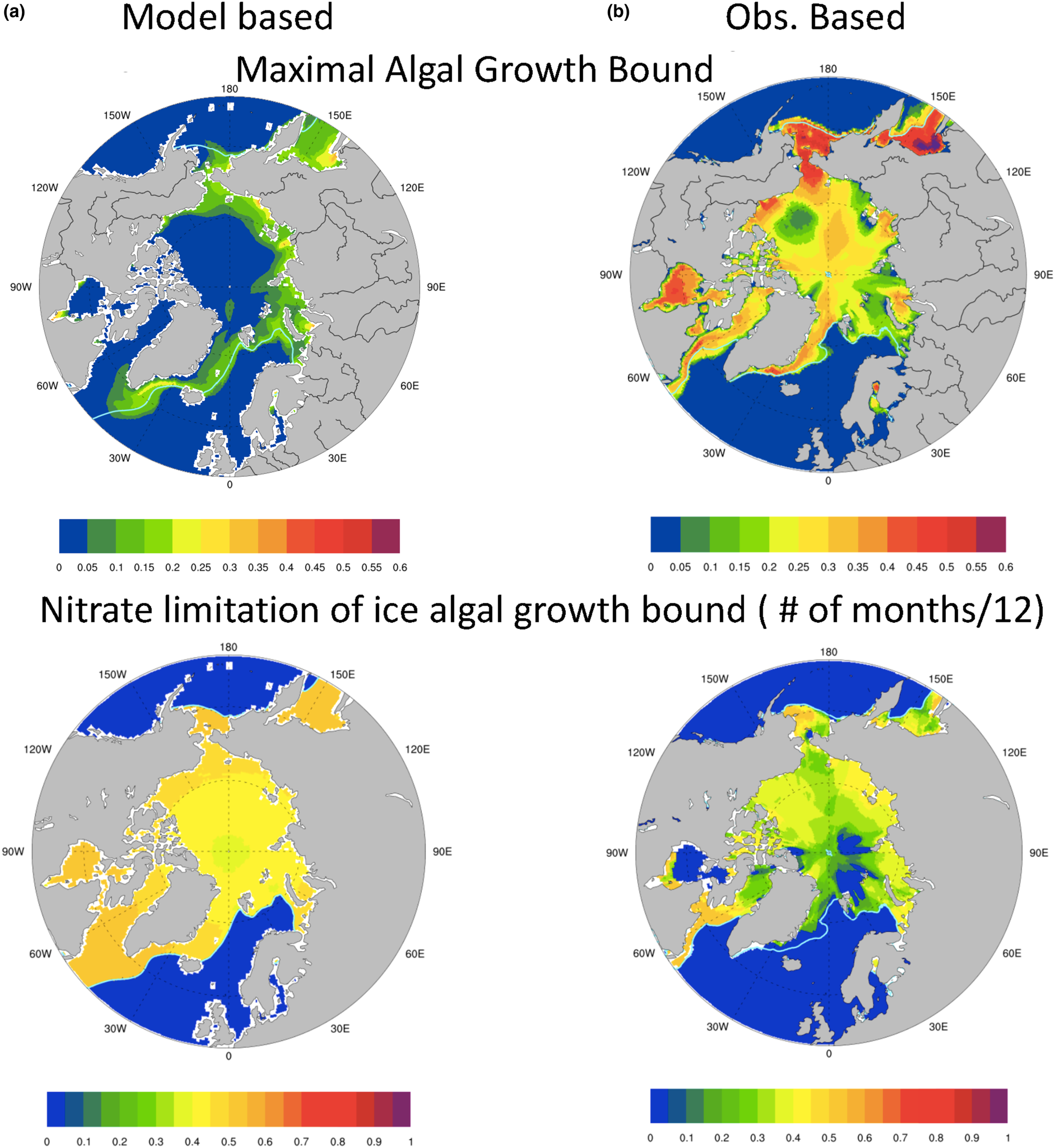
Also shown in Figure 10 (second row) are contour plots of the frequency (fraction of months per year) with which the maximal bound is determined by ocean nitrate concentrations. Given that light necessarily limits growth during the polar night, values of 0.5, which indicate that ocean surface nitrate limits the growth bound for 50% of the year, are extreme. The contours of nitrate limitation frequency based on model output indicate extreme nitrate limitation of the maximal bound throughout the algal growing season. This is reflected in depressed maximal growth rates. The observationally based metric also indicates significant nitrate limitation though not as strong. However, this does not necessarily imply that the computed growth rates from observations are severely depressed. Indeed, nitrate may limit the maximum growth rate in the observational metric, but concentrations are still sufficient to allow moderate (20% of μ max) to high (55% of μ max) algal growth rates.
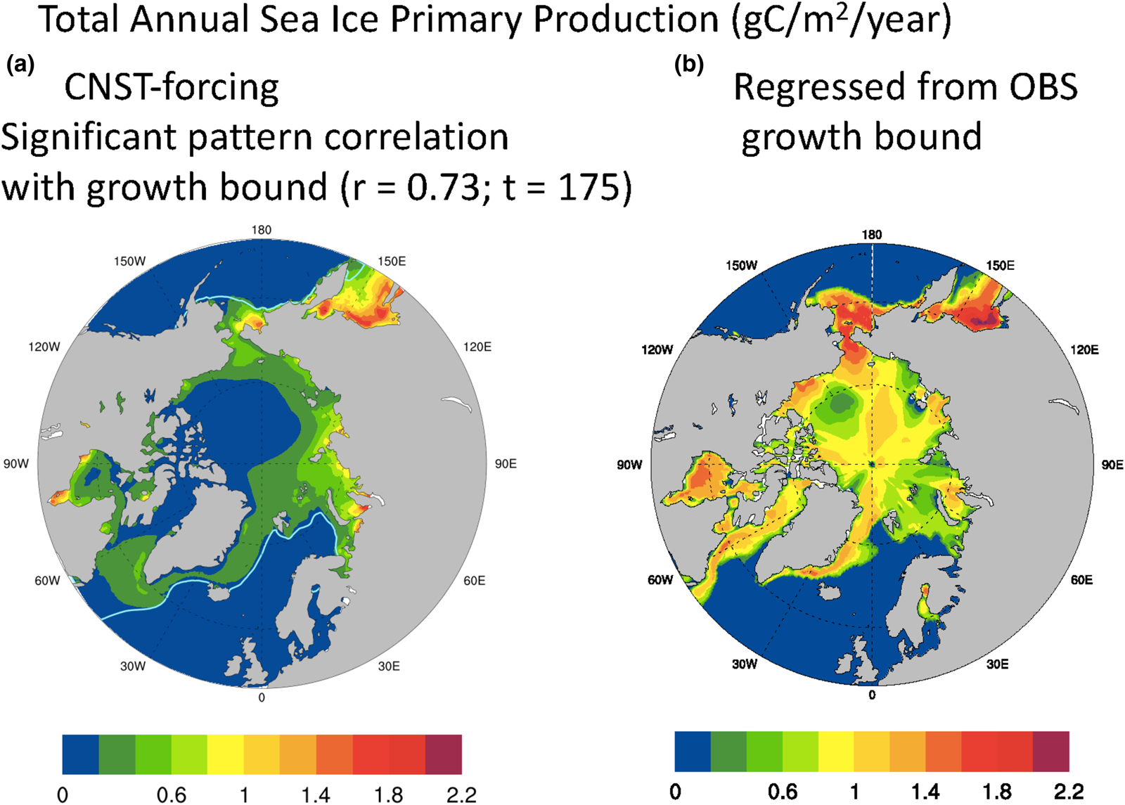
We acknowledge that the maximal growth rate bound as defined above, though useful for contrasting modeled and observed polar states, is a crude measure of sea ice algal growth. Certainly, variability in snow and ice thickness, melt-pond area and in situ nutrient concentrations play significant roles in determining sympagic algal growth rates. Similarly, nitrate limitation of the maximal growth bound does not mean that nitrate is necessarily limiting to the actual algal growth rate. However in the Arctic at least, we do find a significant correlation between the mean net annual ice algal PP of the fully coupled simulation and the maximal growth bound. Conversely, no such pattern correlation is found between mean annual snow thickness and Arctic sea ice primary production. Figure 11a is the total annual sea ice PP averaged over 157 years of CNST-forcing. There are notable similarities with Figure 10a, and indeed the pattern correlation coefficient with the maximal growth rate bound is remarkably high, 0.73 with a t-value of 175. We now use this relationship to improve our estimate of net Arctic PP given the observation-based maximal growth bound. The regressed estimate is shown in Figure 11b. Peak values are similar to the modeled result, but there is far more production along the Canadian shelf and Archipelago, Central Arctic and Bering Sea. Total Arctic PP for the regressed estimate is 60.7 TgC/a, about an order of magnitude larger than the simulated result (Fig. 2) and consistent with the higher estimates of Legendre and others (Reference Legendre1992). The regressed value may be viewed as a model derived estimate of global Arctic sea ice PP that adjusts for ocean nutrient biases in the simulated state. However, it assumes that the pattern correlation between the maximal growth rate bound and PP continues to hold under a state of reduced nitrate limitation.
Mean total annual Arctic primary production (gC/m2/a) in CNST-forcing (a) is significantly correlated with the maximal growth bound of Figure 10. Figure (b) is an estimate of Arctic primary production using the regression coefficient from (a) (r = 0.73) and the observations based on maximal growth bound. Total integrated Arctic ice algal PP from (b) is 60.7 TgC/a. Light blue line indicates the mean 15% sea ice concentration.
A similar analysis for the Southern Ocean is not nearly so useful. Figure 12 shows (a) model-based and (b) observation-based maximal ice algal growth rate bounds for the Southern Ocean. The model-based bound is generally lower than that of observations, ranging between 20 and 80% of μ max, while observations suggest values exceed 50% μ max within the 15% sea ice concentration contour. Certainly, the Southern Ocean modeled polar state appears to be more conducive to ice algal growth than in the Arctic. However, unlike the Arctic, there is no pattern correlation between the maximal growth bound as defined here and net Southern Ocean annual ice PP (r = 0.05). This is because ocean macro-nutrients do not limit the maximal growth bound in the Southern Ocean for either modeled or observed states for any significant fraction of the year (not shown). Rather, incident PAR is always limiting. We find that contrasting algal growth rates based on surface PAR between model and observations, without information about snow and sea ice thickness, is simply too crude a measure. However, the extreme light limitation of the growth bound suggests that snow thickness patterns may provide some clues to regional variability in Southern Ocean ice PP.
Contours of the upper bound for algal growth rate (in units of maximum growth rate, μ max) based on mean annual ocean surface nitrate, silicate and incident PAR from (a) CNST-forcing and (b) observations (references in text). Light blue line indicates the mean 15% sea ice concentration.
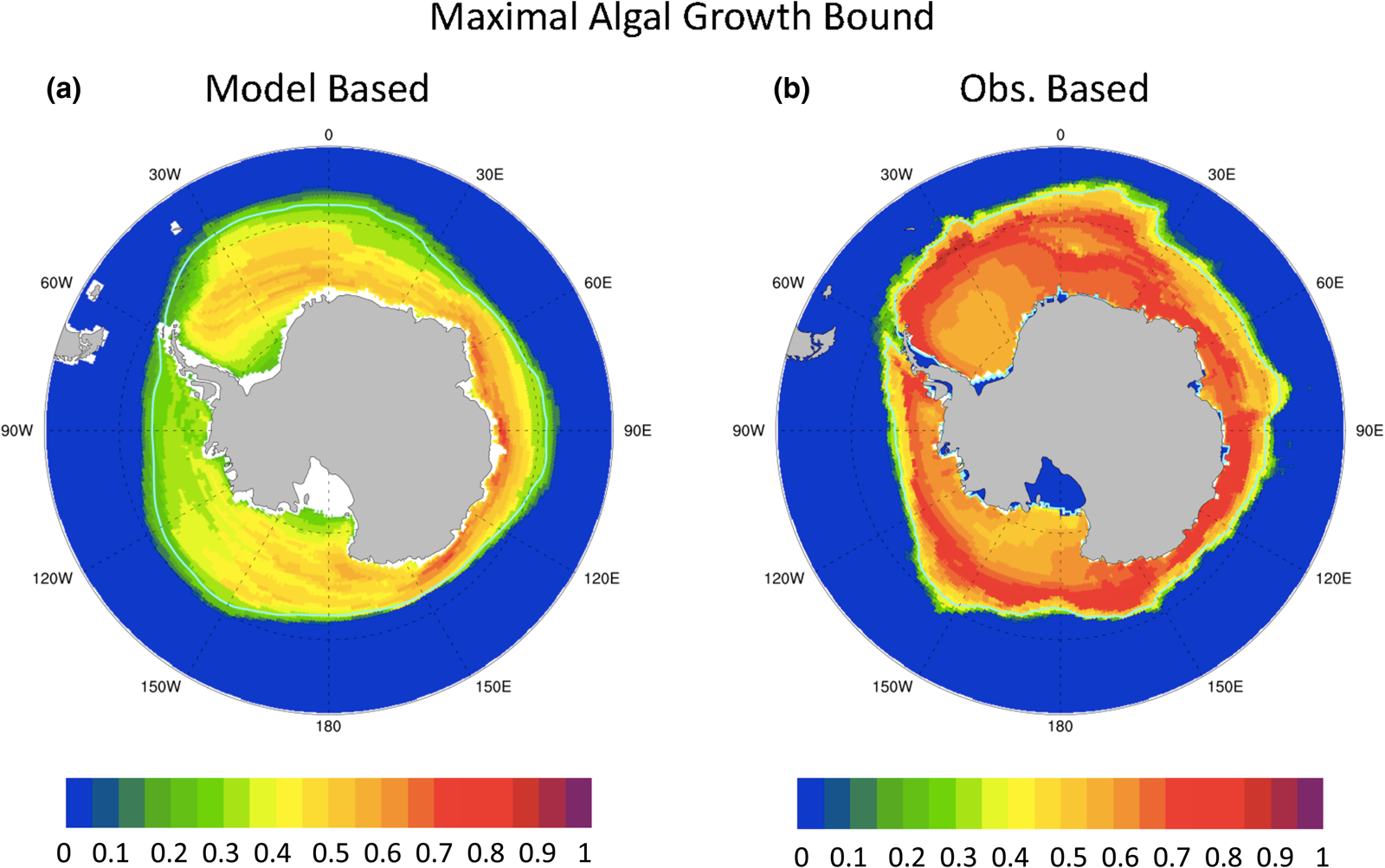
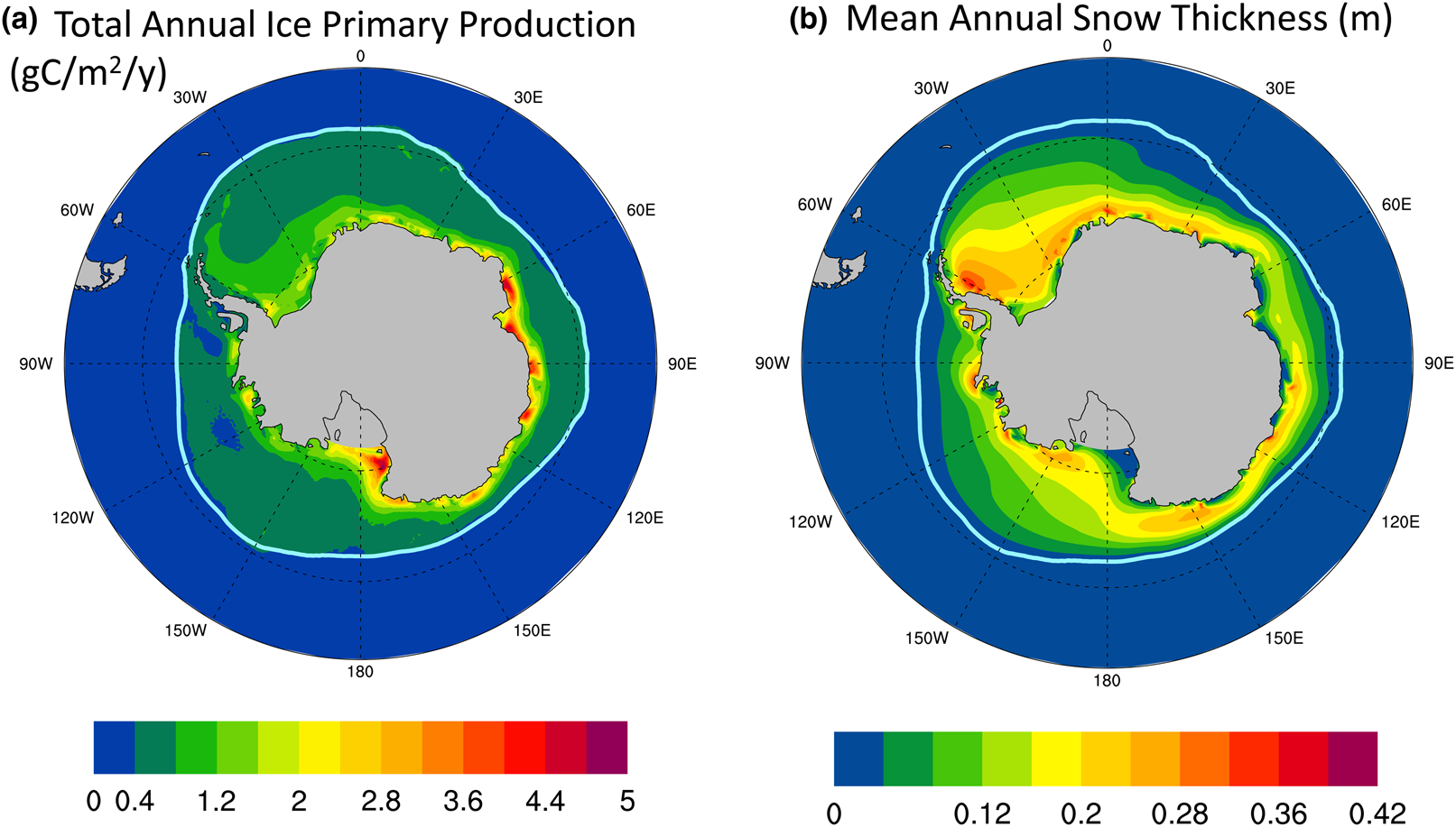
Figure 13a shows the CNST-forcing mean total annual sea ice PP in the Southern Ocean. High production zones generally follow a thin band along the coastline. Figure 13b shows the simulated mean annual snow thickness. There appear to be two regimes: (1) a negatively correlated coastal zone where decreases in snow thickness coincide with increased PP and (2) the pack ice, where snow thickness and net PP in a grid cell (weighted by sea ice area fraction) both correlate positively with sea ice concentration.
(a) Mean total annual primary production in CNST-forcing for the Southern Ocean is uncorrelated with the maximal algal growth bound of Figure 12. However, there are regions, particularly in the coastal zones, where (b) mean snow thickness (m) is negatively correlated with PP. Light blue line indicates the mean 15% sea ice concentration.
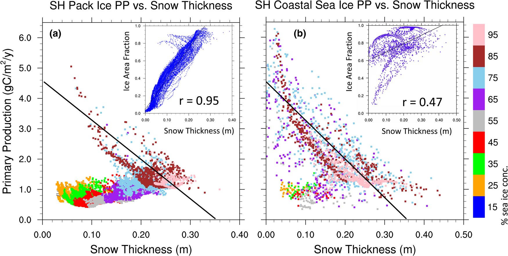
The scatter plots of Figure 14 support these relationships. Figure 14a contains only Southern Ocean sea ice grid points in the deep ocean (ocean depths > 1200 m) which we refer to as the pack ice region. Net annual ice algal PP per sea ice area fraction (note, this is now unweighted by sea ice area fraction) is plotted against mean sea ice thickness and color coded to indicate the mean sea ice concentration of each grid point. For most of the pack ice, snow thickness is positively correlated with sea ice concentration and weakly positive or uncorrelated with primary production. The exception is perennial pack ice where mean annual sea ice concentrations exceed 70–80%. In contrast, for the near coastal sea ice (ocean depths < 1200 m) in Figure 14b, negative correlations between PP and snow thickness are clearly evident when mean sea ice concentrations exceed ~60%. For seasonal ice of the coastal regions, snow thickness again becomes positively correlated with sea ice concentration, and correlations with PP are much weaker. We see similar but notably weaker correlations between sea ice thickness and ice PP (not shown), though this is likely a result of the positive correlation between snow and sea ice thicknesses.
Net annual ice algal primary production per sea ice concentration in a grid cell is plotted against mean sea ice snow thickness and color coded to indicate the mean sea ice concentration. Figure (a) includes only grid cells with ocean depths exceeding 1200 m and (b) includes near coastal grid points with ocean depths < 1200 m. Black lines of equivalent slope (− 12.8 gC/m2/a/m of snow) are shown for reference. Figure inserts are scatter plots of sea ice area concentration versus snow thickness for (a) the sea ice pack and (b) near coastal grid cells. Also shown are correlation coefficients significant at the 99% confidence level.
3.4. Temporal variability in sea ice primary production and chlorophyll-a
In this section, we compare modeled seasonal cycles of sea ice primary production and ice algal chl-a in CNST-forcing with observations. Figures 15 and 16 contrast monthly average PP. For the Arctic, we use the compiled results from Leu and others (Reference Leu2015) plotted as gray shaded bars to denote the time-span and range of observed values. Southern Ocean sea ice PP measurements (Arrigo and others, Reference Arrigo, Mock and Lizotte2010) are very sparse, spanning only three months of the year. Again we use gray shaded bars to indicate the span of observed values. For model results, we compare seasonal cycles of PP using output from the data locations only (blue lines and shading) and for the entire polar region with at least a 15% sea ice concentration (pink lines and shading). Shaded regions indicate the range in monthly mean simulated PP. Also shown is the mean and standard deviation for each month over the CNST-forcing time-series.
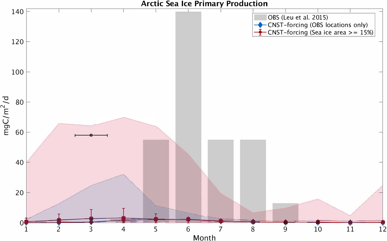
Comparison of monthly average Arctic sea ice primary production in CNST-forcing and observations (Leu and others, Reference Leu2015). Gray shaded regions denote the range of observed values. Colored shaded regions are the range in monthly averaged simulated sea ice primary production for grid cells matching observed locations (blue) and for all grid cells (red). Symbols indicate the mean value over the time-series while error bars denote 1 std. The black square and horizontal bar indicate one reported observation spanning March.
Comparison of monthly average Southern Ocean sea ice primary production in CNST-forcing (blue and red) and observations (gray; Arrigo, Reference Arrigo2003). Gray shaded regions denote the range of observed values. Colored shaded regions are the range in monthly averaged simulated sea ice primary production for grid cells matching observed locations (blue) and for all grid cells (red). Symbols indicate the mean value over the time-series while error bars denote 1 std.
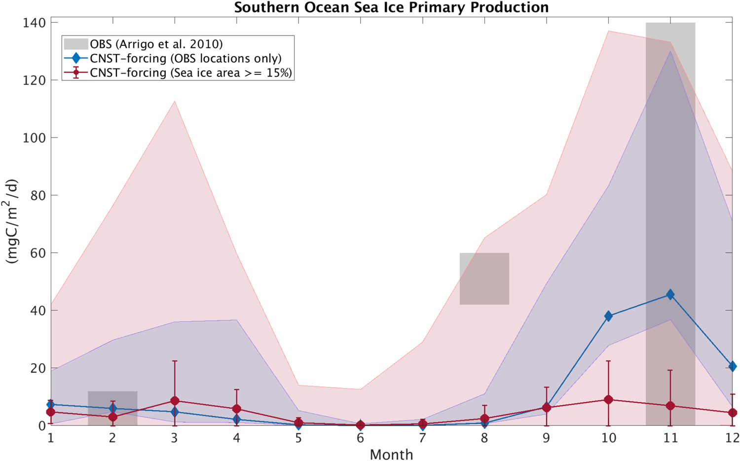
The underestimations in Arctic PP are now clearly evident and are reflected in a reduced and shifted production peak. Observations indicate a June peak, while modeled peak production is in April. This is consistent with severe nutrient limitation in the modeled ocean. The Southern Ocean results, on the other hand, are fairly consistent with observations particularly in the late spring and summer. However, the winter comparison points to possible underestimations in primary production in some regions of the Southern Ocean.
In addition to sea ice column integrated production and chl-a biomass, our model was designed with what we hoped were the important physical processes needed to resolve the vertical ice algal communities: the upper/freeboard communities abundant in the Southern Ocean, interior ice communities, and the bottom or skeletal layer algae common in both the Arctic and Southern Ocean. Figures 17 and 18 show model comparisons with observations of mean sea ice chl-a in each of three vertical regions. For this comparison, we conservatively interpolated vertically resolved observational data and our eight-grid cell vertical output to a 120-layer common vertical grid of normalized depth before averaging into three vertical sections: upper, interior and bottom. Southern Ocean observations are from the ASPeCT data set (Meiners, Reference Meiners2013). Measurements of sectioned core data in the Arctic are less common, in part because PP is found, or assumed to be, primarily in the bottom 3–5 cm. However, measurements from all three vertical sections were obtained from the Bering Sea Ecosystem Study (Gradinger, Reference Gradinger2009), N-ICE2015 (Duarte and others, Reference Duarte2017), Point Barrow (C. Deal pers. comm.) and the Canadian Archipelago (Lange and others, Reference Lange2015).
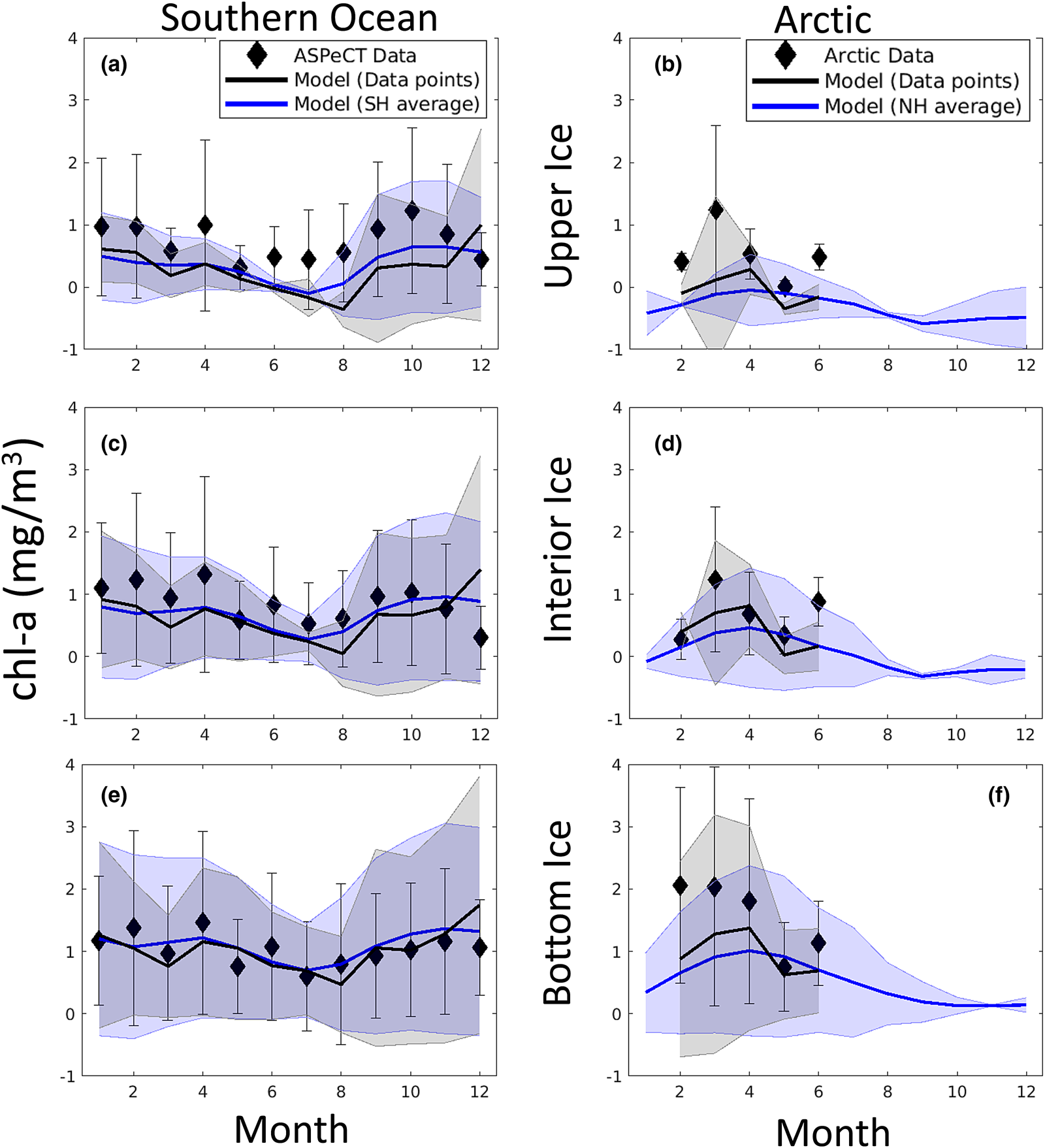
Mean monthly algal chl-a concentrations averaged in the upper (top), interior (middle) and bottom (bottom) thirds of the sea ice column. Measurements and modeled output were first interpolated conservatively to a common 120-layer vertical grid. Symbols and error bars indicate the observed monthly mean concentrations and ± 1 standard for each vertical section. Modeled means and standard deviations are from grid cells corresponding to observed locations (black lines and shading) and all grid cells with sea ice $\gt 15\percnt$ for a given polar region (blue lines and shading). References for observations are given in the text.
Observations and model comparison of the mean fraction of chl-a in a given vertical section of sea ice. See Figure 17 for description of symbols and shading. References for observations are given in the text.
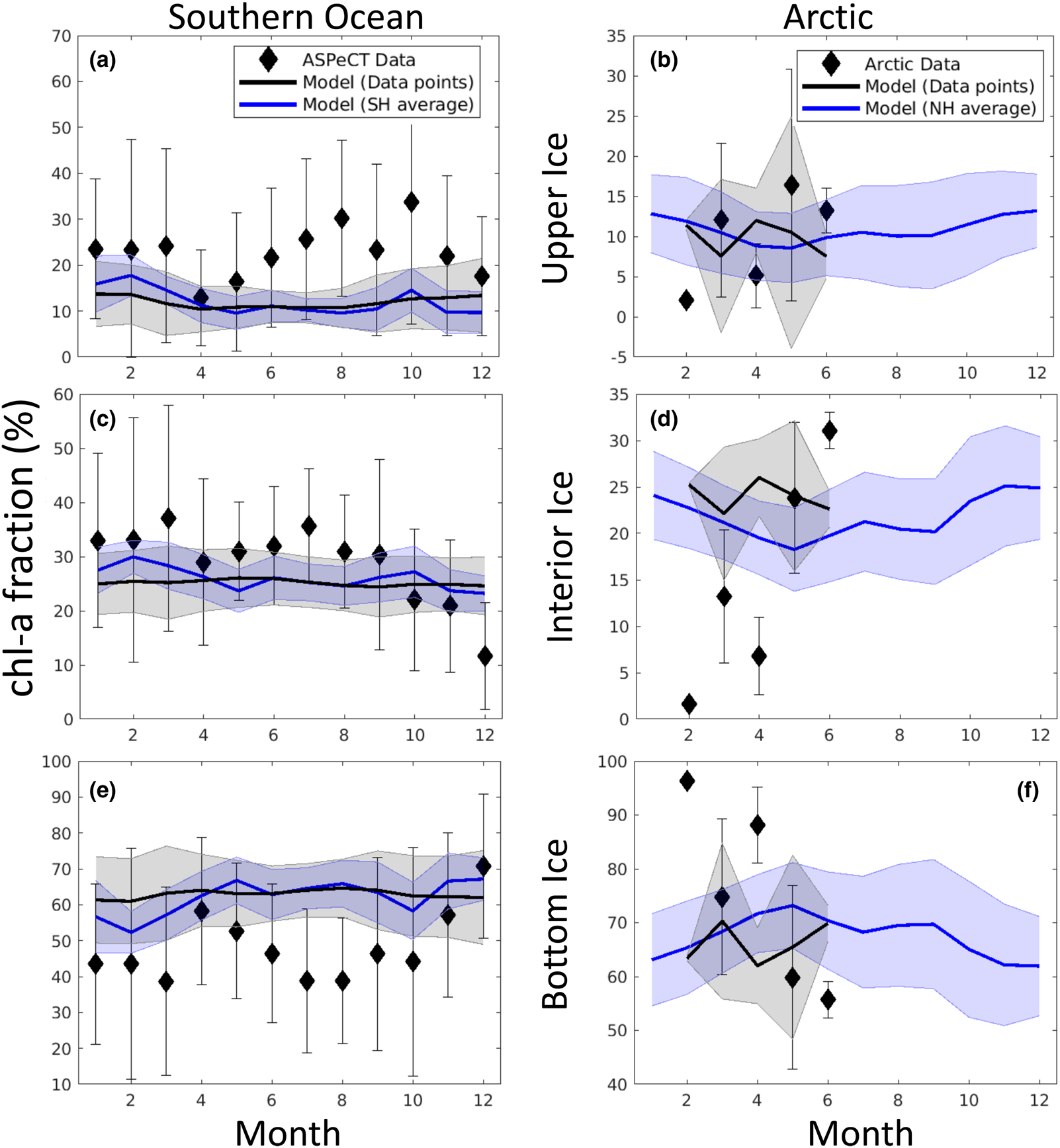
Modeled chl-a concentration averages for vertical sections compare well with observations in both the Arctic and Southern Ocean. This is especially true in the bottom and interior ice, but less so in the upper ice. In particular, Southern Ocean upper ice concentrations are underestimated, though by less than 1 mg chl-a/m3, during the winter months. The March peak in Arctic chl-a in observations is due to the Bering sea region which is disproportionately represented in the profile data set. Our model indicates an April peak in Arctic mean chl-a. However, this later peak is also evident in mean simulated chl-a computed from the grid locations of corresponding core observations. This suggests model biases in the Bering Sea, possibly in the timing of sea ice retreat.
Figure 18 is more revealing. Here the fraction of chl-a in a given vertical section is computed before averaging. Upper ice communities in the Southern Ocean comprise, on average, between 12 and 35% of the ice core during an annual cycle. Our model means are between 10 and 19%, underestimating upper ice communities in the Southern Ocean. Modeled chl-a, rather, favors the bottom ice layer, attributing 50–70% of total chl-a biomass. Observations indicate a lower range (40–60%) for 11 months of the year. Observations of Arctic chl-a profile fractions exhibit greater variability in seasonality than in the simulated climatology. This is in part expected given the paucity of data. Simulated mean profiles do not well represent observed profiles with very high bottom ice concentrations (e.g. February and April). The model tends to spread out this biomass among the layers. This is not surprising given that the model uses only eight grid levels and numerical diffusion is high. Simulated monthly mean bottom ice fractions range between 60 and 70% between February and March while observations suggest values > 90% in March to ~55% in June. Note that we have likely underestimated the contribution of observed ice cores with very high bottom chl-a, given that we did not use data if upper and interior ice measurements were not made or not reported.
Given the observed relationships between modeled ocean surface nitrate (via the maximal growth rate bound) and PP in the Arctic, and between snow thickness and PP in the Southern Ocean, it is perhaps not surprising that we also see correlations in the CNST-forcing time-series anomalies (annual value minus its time-series mean) of these observables. Figures 19a and b show contours of the Pearson correlation coefficient between anomalies of ice algal annual net PP and annual mean surface nitrate in the Arctic and Southern Ocean, respectively. Only significant correlations at the 95% confidence level are shown. Strong positive correlations are evident in much of the western and central Arctic. Not surprisingly, Southern Ocean PP anomalies are poorly correlated with surface nitrate anomalies except just beyond the mean 15% concentration ice edge. Here, positive anomalies in algal PP result in additional draw-down of nitrate and hence significant negative correlations with ocean surface concentrations.
Contours of the Pearson correlation coefficient (r) between the anomalies of (a,b) ice algal annual net primary production (PP) and annual mean ocean surface nitrate (NO3) and the anomalies of (c,d) ice algal annual net primary production and annual mean snow thickness (hs). Only significant values at the 95% confidence level are shown. The red line is the mean sea ice 15% contour.
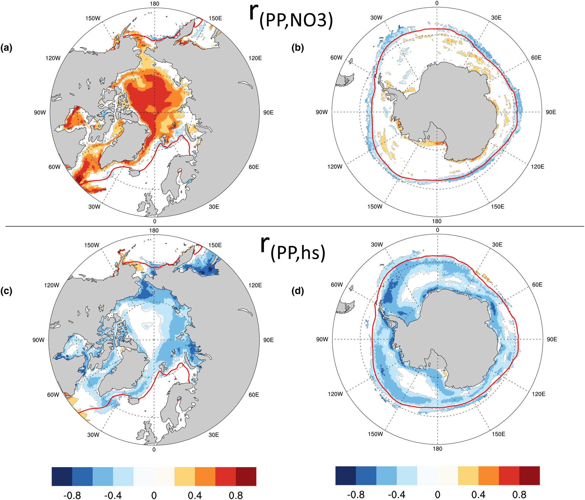
In both the Arctic and Southern Ocean, snow thickness anomalies are negatively correlated with anomalies in annual net algal primary production (Figs 19c and d). This is particularly true in regions of modeled higher production such as the Eastern Siberian Sea and Sea of Okhotsk and in the near coastal band of the Southern Ocean.
4. Discussion
Global time-series of E3SMv1.1-BGC pre-industrial and historical simulations support the lower bound in previous estimates of net sea ice PP in both polar regions, with an Arctic mean value of 7.5 TgC/a and a Southern Ocean mean of 15.5 TgC/a. However, closer analysis of simulated polar climate and comparisons with in situ primary production measurements suggest, rather, that the Arctic lower bound estimate is a significant underestimation driven in large part by biases in surface ocean nitrate. In addition, our analysis indicates that improved surface nitrate representation would augment the simulated net Arctic ice algal PP with a capacity corresponding to 60.7 TgC/a, which is more consistent with the upper bound suggested by Legendre and others (Reference Legendre1992).
In contrast, model simulations of chl-a biomass (concentrations and column integrated values) are broadly consistent with observations in both poles. This provides some support for our algal vertical transport parameterizations, particularly algal motility which alters chl-a concentrations while preserving column integrated values. With respect to vertical algal communities, we see moderate agreement in mean chl-a concentrations for interior and bottom ice though with greater uniformity in the simulated profiles. This is in part due to poor vertical resolution and excessive numerical diffusion.
The biases in chl-a profile fractions, however, indicate that we have difficulty representing cores with high algal biomass in the bottom layer, and that we continue to underestimate the upper and freeboard communities of the Southern Ocean. The latter is notable because upper ice algal production is supported by processes somewhat distinct from bottom communities, which depend heavily on gravity drainage exchange with the ocean. That is, we expect surface flooding, snow loading and remineralization to play larger roles. Our model treats these processes rather simply. First, we neglect all surface flooding from lateral flow and macro-scale porosity features in the ice, though this is an observed phenomenon (Eicken and others, Reference Eicken, Lange, Hubberten and Wadhams1994), because developments to include macro-porosity in MPAS-Seaice are ongoing. We do, however, expect that this additional surface flooding enhances upper ice nitrate and correspondingly chl-a concentrations relative to the bottom and interior values.
Snow loading, which is modeled as pressure-driven flow through a porous medium using Darcy's law, has only one tunable parameter: the snow porosity. Measured values range significantly from less than 0.3 for very wet snow to 0.95 for newly fallen snow (Singh and others, Reference Singh, Kumar, Venkataraman, Rao and Mani2007), and it may be that a dynamic value based on snow aging is appropriate. Indeed, (Jeffery and Hunke, Reference Jeffery and Hunke2014) found that brine salinity accumulated in upper ice/snow layers during simulated snow loading events was highly sensitive to this parameter. Currently, developments are underway to add snow aging to MPAS-Seaice for E3SMv2.
The question remains, are significant underestimations in Arctic sea ice algal PP consistent with reasonable representations of chl-a? If not, what do these inconsistencies imply about our ice biogeochemical model? In our simulations, Arctic ice PP is underestimated because of constraints to specific growth rate and not algal biomass. Certainly, low PP is not by definition inconsistent with accurate chl-a estimates. Sea ice column integrated chl-a, on the other hand, is a result of a balance of fluxes: (1) primary production, which is an inorganic carbon (nitrogen) to algal carbon (nitrogen) flux; (2) ocean to ice algal chl-a fluxes, which though small compared with (1), are responsible for seeding of the sea ice algal community; (3) ice to ocean melt fluxes; and (4) grazing and mortality losses. Given that PP is the dominant positive flux, accurate chl-a can only be achieved with compensatory negative fluxes, i.e. underestimations of grazing and mortality and/or ice to ocean melt losses. Indeed, as we indicated in section: Tuning and model parameters, both the grazing fraction (zero for diatoms though 0.7 for small plankton and Phaeocystis sp.) and the algal mortality rate (0.007 1/d for all algal groups) were reduced during the tuning process. Further, the tuned values for attachment and desorption time-scales served to maximize ocean to ice chl-a accumulation and reduce ice to ocean losses during melt. We expect that in reality the Arctic ice algal system experiences up to an order of magnitude higher turnover rates.
Validity of our Southern Ocean net PP estimate is more difficult to assess, because there are too few ice algal production measurements available. Comparisons are favorable, but they do suggest that the model may underestimate production in winter. With respect to the modeled polar climate, we again see ocean surface macro-nutrient (nitrate and silicate) biases, though these do not exert a limiting control on Southern Ocean ice PP. Rather incident PAR and snow thicknesses play important roles. Unfortunately, it is difficult to validate modeled snow thickness, particularly in the coastal band of high PP, because current methods of snow depth retrieval are poor in regions of high ice compaction and ridging (Kern and Ozsoy-Çiçek, Reference Kern and Ozsoy-Çiçek2016). Still, we know that upper and freeboard ice algal chl-a fractions are underestimated and this implies, at the very least, insufficient sea ice PP in the upper layers relative to the bottom ice. In addition, our model does not include platelet ice layers which are known to support some of the highest rates of sea ice PP in the Southern Ocean (Arrigo and others, Reference Arrigo, Mock and Lizotte2010).
Certainly, the modeling of ice algal systems would benefit greatly from additional measurements of ice algal PP rates, particularly those which enhance the regional and temporal coverage of both polar regions. There is also a need for measurements which constrain losses such as grazing rates and ice–ocean exchanges of organic material throughout the seasonal cycle. Additional remineralized sources of nitrogen may play a particularly important role in supporting ice algal communities, especially during periods of the year when sea ice physics places constraints on ocean–ice fluxes. We acknowledge that our simplified treatment of remineralization and nitrogen cycling in sea ice likely contributes to underestimations in PP in both polar regions. Specifically, we do not include remineralization of dissolved organic nitrogen (DON), although the work of Fripiat and others (Reference Fripiat2014) and Fripiat and others (Reference Fripiat, Sigman, Massé and Tison2015) indicates that DON incorporation into sea ice during winter and subsequent sympagic remineralization provides an important supplemental source of nitrogen to ice algae. In future work, we plan to improve sympagic nitrogen cycling with explicit remineralization of DON and nitrification, with the caveat that adequate measurements of ice–ocean DON fluxes in addition to remineralization rates will be essential for model validation.
5. Conclusion
Coupling of the 3D sea ice algal model, MPAS-Seaice zbgc, into the E3SMv1.1 global climate system enables comparative investigation of Arctic and Southern Ocean sea ice PP. We have assumed that ice algal dynamics in both poles is described by a common set of biogeochemical exchanges and that differences in ice chl-a and primary production can be explained by variations in environmental conditions. For our analysis, we consider 180 years of simulated pre-industrial and historical environmental variability. Interpreting the results of climate model output is challenging, and conclusions often reflect the peculiarities of a particular model rather than the natural system we are trying to understand. Our approach is to first define a simple metric, a maximal bound for algal growth rate, that assesses the quality of both the modeled and observed polar states as it pertains to sea ice algae. In this way, light and surface nutrient biases are only relevant if and when they limit the algal growth bound. Our approach is not unique. Horvat and others (Reference Horvat2017) use a more sophisticated metric for light limitation that includes albedo changes from melt-pond formation. However, we choose a metric that can be evaluated from readily available observations as well as generic model output.
We find that biases in simulated surface ocean nitrate lead to large differences in the regional patterns of the maximal algal growth bound between mean simulated and observed Arctic environments. In effect, we see potential suppression of simulated ice algal growth rates to < 5% of μ max in the central and Canadian Arctic, whereas observations suggest moderate suppression to ~30% of μ max and coastal values as high as 55% of μ max. The metric does not contain information about sea ice biogeochemical or physical processes, aside from the mean monthly 15% ice concentration contour and a common set of algal growth limitation functions, but we observe a positive pattern correlation coefficient of 0.73 between the bound and net sea ice algal primary production from the fully coupled model. Although we expect the correlation to grow weaker with reduced surface nitrate biases, we estimate using the observation-based maximal algal growth bound that net Arctic PP may be as high as 60.7 TgC/a.
In contrast, the maximal algal growth bound in the Southern Ocean is not correlated to sea ice algal PP. Rather, the metric confirms what is well known, that ocean surface macro-nutrients are abundant, and that functions of incident PAR are not sufficient proxies for ice algal growth. However, strong light limitation of the bound in both observations and simulations indicates that variations in snow thickness play a likely role in regional patterns of PP. Indeed, we observe strong negative pattern correlations in the model between snow thickness and Southern Ocean PP, particularly in the high-production perennial ice of coastal Antarctica. In contrast, pack ice is generally uncorrelated or weakly positively correlated with PP, except for regions of high mean annual ice concentrations (> 70%).
Finally, we investigate two potential sources of inter-annual variability in pre-industrial sea ice PP: ocean surface nitrate anomalies and sea ice thickness anomalies. Not surprisingly, we see significant positive correlations in Arctic surface nitrate and primary production anomalies for much of the central and Canadian Arctic where the maximal growth bound is strongly suppressed from nitrate limitation. Conversely, Southern Ocean PP variability is generally not driven by nitrate concentrations. Rather, anomalous increases in ice PP beyond the mean 15% ice extent contour are correlated with decreases in surface ocean nitrate, which is responding to the additional nitrogen demand. Snow thickness anomalies, however, are negatively correlated with algal PP for both poles, indicating that light limitation is also an important control on Arctic PP. Significant negative correlations are particularly evident in the higher ice PP zones for both regions. The exception is a band in the Southern Ocean, southward of the sea ice edge, where net ice PP is low because of low mean sea ice concentrations. However, ice algal growth rates are high, light-limited and sensitive to snow thickness variability.
Acknowledgments
This research was supported as part of the Energy Exascale Earth System Model (E3SM) project, funded by the US Department of Energy, Office of Science, Office of Biological and Environmental Research. Additional support was provided by the Reducing Uncertainties in Biogeochemical Interactions through Synthesis and Computation (RUBISCO) Scientific Focus Area (SFA), which is sponsored by the Regional and Global Model Analysis (RGMA) Program in the Climate and Environmental Sciences Division (CESD) of the Office of Biological and Environmental Research in the US Department of Energy Office of Science. The National Center for Atmospheric Research is a major facility sponsored by the National Science Foundation under Cooperative Agreement No. 1852977. The authors thank all the members of the E3SM project for their essential contributions and support. Special thanks to S. Elliott and two anonymous reviewers for their many insightful comments.
APPENDIX A. Brine evolution
Motion of the brine level (h b) is fundamentally a result of gravitational forces and depends on the permeability of the ice, changes in the ice bottom and surface boundaries, and surface sources of water: snow and ice meltwater, sea water flooding and liquid precipitation. Computation of h b at t + Δt is a two-step process. First, h b is updated from changes in ice (h i) and snow thickness (h s), i.e.
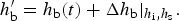
The contribution $\Delta h_{\rm b}\vert _{h_{\rm i}\comma h_{\rm s}}$ arises from snow and ice melt and bottom ice growth. Since the ice and brine bottom boundaries coincide, changes in the ice bottom from growth or melt, (Δh i|bot), equal the bottom brine boundary changes. The surface contributions from ice (Δh i|top) and snow melt (Δh s|melt), however, are opposite in sign since an ice/snow to liquid conversion above the brine level adds to the total fluid volume. As an initial simplification, we do not assume any direct runoff into the ocean although this is certainly possible particularly in areas of low ice concentration.
The brine level change from snow melt and ice thickness changes is

The symbol ρ is density and the subscripts i, s and b correspond to ice, snow and brine, respectively. In the second step, we apply pressure-driven adjustments arising from meltwater flushing and snow loading to h′b. Brine flow due to pressure forces are governed by Darcy's equation for the boundary velocity, w (Fetter, Reference Fetter2001):
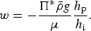
where μ is the viscosity, g is the gravitational acceleration and $\bar {\rho }$ is the average sea ice density. The ice thickness, h i, the hydraulic head, h p, and the vertical component of the net permeability, $\Pi ^\ast$
 , depend on the ice state and are computed at each time step. The hydraulic head is h p = h′b − h sl with h sl equal to the sea level relative to the ice bottom (see Jeffery and others (Reference Jeffery, Hunke and Elliott2011) for further details).
If we assume that changes in h i and h s are negligible while Darcy flow adjusts the bulk brine level, then the rate of change of h b from pressure forces (indicated by |pr) is

with $w_{\rm o} = \Pi ^\ast \bar {\rho } g/\lpar h_{\rm i}\mu \phi _{{\rm top}}\rpar$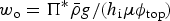 and ϕtop the surface porosity. When Darcy flow is downward into the ice (w o < 0), ϕtop equals the sea ice porosity in the uppermost layer. When the flow is upwards into the snow, then ϕtop equals the snow porosity (ϕ top = 1 − ρ s/ρ w).
Since h sl remains relatively unchanged during Darcy flow, (A4) has the approximate solution

Together equations A2 and A5 define the vertical domain of the zbgc model at each time step relative to the ice state grid and provide essential information to compute the impact of brine flushing on biogeochemical tracers.
APPENDIX B. Biogeochemical reaction terms
The biochemical reaction terms, R([c]) (or more concisely R c) in (4), are generally non-linear, vertically resolved functions of ice temperature, salinity, photosynthetically active radiation (PAR) and tracer brine concentrations. For each algal species (represented by $\hbox {N}$ to indicate units of algal nitrogen concentration), $R_{\hbox {N}}$
 has the form:

where the algal growth rate μ is in general a function of PAR, temperature and the limiting nutrient. f graze is the fraction of algal growth that is lost to predatory grazing, and f res is the fraction of algal growth lost to respiration. Algal mortality, M ort, is temperature dependent and modeled after (Arrhenius, Reference Arrhenius1889), but also limited by a maximum loss rate fraction (l max):

where [ · · · ] denotes brine concentration. The parameters m pre and m T are the maximum mortality rate and mortality temperature decay, respectively.
Nitrate and ammonium reaction terms are given by
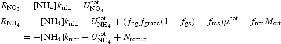
where the uptake U tot and algal growth μ tot are accumulated totals for all algal species. k nitr is the nitrification rate, f ng and f nm are the fractions of grazing and algal mortality that are remineralized to ammonium, and f gs is the fraction of grazing spilled or lost. Algal uptake and growth rates are described in detail in the next section.
Silicate, an essential nutrient for diatom growth but not required by small plankton or Phaeocystis sp., has no biochemical source terms within the ice and is lost only through algal uptake:
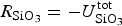
Dissolved iron, on the other hand, has both algal uptake and remineralization pathways. The current model configuration does not include conversions between particulate and dissolved iron species. This is in part because the ocean model does not carry an explicit particulate iron pool nor are there sources of sedimentary iron near shelf and coastal regions, and neither model prognoses or derives ligand concentration. Despite this shortcoming, even a simplified dissolved iron dependency in sea ice provides a means to begin assessing the role of physical ice–ocean mechanisms in the observed accumulation of biologically available iron in polar regions.
The full equation for dFe including uptake and remineralization is
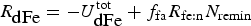
where R fe:n is the ratio of iron to nitrogen in the remineralized pool and f fa is the fraction retained as dissolved iron.
See Table II for a more complete list and description of biogeochemical parameters.
APPENDIX C. Algal growth and nutrient uptake
Algal growth rates depend upon available PAR and follow Liebig's Law of the minimum, which states that growth is controlled by the scarcest resource. Limitation factors are first computed for light (L lim) and each of the potentially limiting nutrients, NO3, NH4, SiO3 and dFe, to determine the greatest impediment to growth. The maximum growth rate at a given temperature is then reduced by the limiting factor to compute the true growth rate μ. Nutrient uptake rates are then calculated based on the true growth rate. Care must be taken with multiple algal species to insure that total uptake in a given time step does not deplete brine concentrations below a minimum threshold fraction.
Nutrient limitation terms obey the Michaelis–Menten equations:
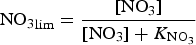
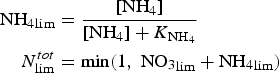
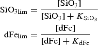
with specified half-saturation coefficients K x for a given nutrient X.
Light limitation L lim is defined in the following way: I sw(z) (in W/m 2) is the shortwave radiation at the ice depth z. The optical depth is proportional to the chl-a concentration, $op_{{\rm dep}} = chlabs [{\hbox{Chl}a} ]$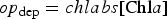 . If (op dep > op min) then, after (Sakshaug and others, Reference Sakshaug, Andresen and Kiefer1989),

otherwise I avg = I sw.

with exponential light limitation after (Martinez and others, Reference Martinez, Camacho, Jimenez and Espinola1997) parameterized by α, and limitation modeled as first-order decay kinetics with factor β (Kok, Reference Kok1956).
The maximal algal growth rate before limitation is a function of temperature T (Ahlgren, Reference Ahlgren1987):

and

is the initial estimate of algal growth rate for a given algal species. ΔT is the difference between the local and the maximum temperatures (in this case Tmax = 0°C).
The initial estimate of the uptake rate for silicate and dissolved iron (denoted by tilde) is computed assuming an algal-type specific silica to nitrogen ratio (R si:n) and iron to nitrogen ratio (R fe:n):
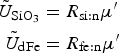
For nitrogen uptake, we assume that ammonium is preferentially acquired by algae. For each algal growth rate, μ, first determine the maximum potential uptake rate of ammonium based on its limitation factor:
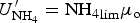
Then determine the uptake based on the initial estimate μ′ (C15)
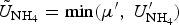
and satisfy the remaining nitrogen demand by nitrate acquisition.
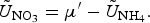
We require that each rate not exceed a maximum loss rate l max/dt.This is particularly important when multiple species are present. In this case, the accumulated uptake rate for each nutrient is found and the fraction (fU i) of uptake due to algal species i is saved and maintained in what follows. The total uptake rate is compared with the maximum loss condition and the lower value chosen. For example, the net uptake of nitrate when there are three algal species is
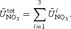
Then the uptake fraction for species i and the adjusted total uptake is
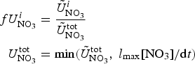
Now, for each algal species the nitrate uptake is
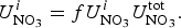
Similar expressions are found for all potentially limiting nutrients. Then the true growth rate for each algal species i is

Preferential ammonium uptake is assumed once again and the remaining nitrogen is taken from the nitrate pool.


 Open access