


1. Introduction
Turbulent flows with two layers are ubiquitous in nature and technology: for example, the coupled flows between the ocean and the atmosphere (Neelin, Latif & Jin Reference Neelin, Latif and Jin1994), the convection of the Earth's upper and lower mantles (Tackley Reference Tackley2000), oil slicks on the sea (Fay Reference Fay1969) and even cooking soup in daily life. Compared with flow with only a single layer, multilayer flow has more complicated flow dynamics and thus more complicated global transport properties. These are determined by the viscous and thermal coupling between the fluid layers. In order to investigate the heat transport in two-layer thermal turbulence, we choose turbulent Rayleigh–Bénard (RB) convection as our canonical model system. The main question to answer is: How does the global heat transport depend on the ratios of the fluid properties and the thicknesses of the two layers?
Rayleigh–Bénard convection, where a fluid is heated from below and cooled from above, is the most paradigmatic example in the study of global heat transport in turbulent flow (see the reviews of Ahlers, Grossmann & Lohse (Reference Ahlers, Grossmann and Lohse2009), Lohse & Xia (Reference Lohse and Xia2010), Chillà & Schumacher (Reference Chillà and Schumacher2012) and Shishkina (Reference Shishkina2021)). Also, previous studies on multiphase flow have taken RB convection as their model system; for example, the studies on boiling convection (Zhong, Funfschilling & Ahlers Reference Zhong, Funfschilling and Ahlers2009; Lakkaraju et al. Reference Lakkaraju, Stevens, Oresta, Verzicco, Lohse and Prosperetti2013; Wang, Mathai & Sun Reference Wang, Mathai and Sun2019), ice melting in a turbulent environment (Wang et al. Reference Wang, Calzavarini, Sun and Toschi2021) or convection laden with droplets (Pelusi et al. Reference Pelusi, Sbragaglia, Benzi, Scagliarini, Bernaschi and Succi2021; Liu et al. Reference Liu, Chong, Ng, Verzicco and Lohse2022). These are mainly dispersed multiphase flow. Here we focus on two-layer RB convection, which is highly relevant in geophysics and industrial applications.
Most studies on two-layer RB convection have hitherto been conducted in the non-turbulent regime (Nataf, Moreno & Cardin Reference Nataf, Moreno and Cardin1988; Prakash & Koster Reference Prakash and Koster1994; Busse & Petry Reference Busse and Petry2009; Diwakar et al. Reference Diwakar, Tiwari, Das and Sundararajan2014), while only a few studies focused on the turbulent one: Davaille (Reference Davaille1999) experimentally studied RB convection with two miscible layers and displayed the temperature profiles in each layer and the deformation of the interface. Experiments of RB convection with two immiscible fluid layers were reported by Xie & Xia (Reference Xie and Xia2013), who quantified the viscous and thermal coupling between the layers and showed that the global heat flux weakly depends on the type of coupling, i.e. the heat flux at viscous coupling normalized by that at thermal coupling varies from  $0.997$ to $1.004$.
Next to the experiments, the numerical study by Yoshida & Hamano (Reference Yoshida and Hamano2016) focused on the heat transport efficiency in two-layer mantle convection with large viscosity contrasts. Our prior numerical simulations (Liu et al. Reference Liu, Chong, Wang, Ng, Verzicco and Lohse2021a) explored a wide range of Weber numbers and density ratios between the two fluids and revealed the interface breakup criteria in two-layer RB convection. Also, most previous studies have focused on the flow dynamics and behaviour of the interface between the two layers. The issue of global heat transport is still quite unexplored, especially in the turbulent regime.
In the present work, we numerically investigate RB convection through two immiscible fluid layers by two-dimensional (2-D) and three-dimensional (3-D) direct numerical simulations. We first calculate the global heat transport for various layer thicknesses and fluid properties. In addition, we extend the Grossmann–Lohse (GL) theory for standard RB convection to the two-layer system and are able to predict the heat transport of the system. The GL theory (Grossmann & Lohse Reference Grossmann and Lohse2000, Reference Grossmann and Lohse2001, Reference Grossmann and Lohse2002; Stevens et al. Reference Stevens, van der Poel, Grossmann and Lohse2013) is a unifying theory for the effective scaling in thermal convection, which successfully describes how the Nusselt number  $\mbox {Nu}$ and the Reynolds number $\mbox {Re}$ depend on the Rayleigh number $\mbox {Ra}$ and the Prandtl number $\mbox {Pr}$. This theory has been well validated over a wide parameter range by many single-phase experimental and numerical results (Stevens et al. Reference Stevens, van der Poel, Grossmann and Lohse2013). We show that the predictions from the GL theory can be extended to two-layer systems without introducing any new free parameter, and the extended theory agrees well with our numerical results and with previous experimental data (Wang et al. Reference Wang, Mathai and Sun2019). The GL theory also successfully gives the mean temperature at the interface between the two layers.
The organization of this paper is as follows. The numerical method and set-up are introduced in § 2. The main results are presented in §§ 3–5; namely the flow structure and heat transfer in the two-layer RB convection in § 3, the temperature at the interface in § 4 and the effects of the interface deformability on the heat transfer in § 5. The paper ends with conclusions and an outlook.
2. Numerical method and set-up
In this study, 2-D and 3-D simulations are performed. We consider two immiscible fluid layers (fluid 2 over fluid 1) placed in a domain of dimensions  $2H\times 2H\times H$ in three dimensions and $2H\times H$ in two dimensions, with $H$ being the domain height. The numerical method (Liu et al. Reference Liu, Ng, Chong, Verzicco and Lohse2021b) used here combines the phase-field method (Jacqmin Reference Jacqmin1999; Ding, Spelt & Shu Reference Ding, Spelt and Shu2007; Liu & Ding Reference Liu and Ding2015) and a direct numerical simulation solver for the Navier–Stokes equations (Verzicco & Orlandi Reference Verzicco and Orlandi1996; van der Poel et al. Reference van der Poel, Ostilla-Mónico, Donners and Verzicco2015), namely AFiD. This method has been well validated in our previous study (Liu et al. Reference Liu, Ng, Chong, Verzicco and Lohse2021b).
In the phase field method, which is widely used in multiphase simulations of laminar (Chen et al. Reference Chen, Liu, Gao and Ding2020; Li, Liu & Ding Reference Li, Liu and Ding2020) and turbulent flows (Roccon, Zonta & Soldati Reference Roccon, Zonta and Soldati2019, Reference Roccon, Zonta and Soldati2021), the interface is represented by contours of the volume fraction  $C$ of fluid 1. The corresponding volume fraction of fluid 2 is $1-C$. The evolution of $C$ is governed by the Cahn–Hilliard equation,
 \begin{equation} \frac {\partial C} {\partial t} + \boldsymbol{\nabla} \boldsymbol{\cdot} ({\boldsymbol u} C) = \frac{1}{\mbox{Pe}}\nabla^2 \psi, \end{equation}
where  $\boldsymbol u$ is the flow velocity and $\psi = C^{3} - 1.5 C^{2}+ 0.5 C -\mbox {Cn}^{2} \nabla ^2 C$ the chemical potential. We set the Péclet number $\mbox {Pe}=0.9/\mbox {Cn}$ and the Cahn number $\mbox {Cn}=0.75h/H$, where $h$ is the mesh size. We take $\mbox {Pe}$ and $\mbox {Cn}$ according to the criteria proposed in Ding et al. (Reference Ding, Spelt and Shu2007), Yue, Zhou & Feng (Reference Yue, Zhou and Feng2010) and Liu & Ding (Reference Liu and Ding2015), which approaches the sharp-interface limit and leads to well-converged results with mesh refinement. More numerical details, validation cases and convergence tests can be found in Liu et al. (Reference Liu, Ng, Chong, Verzicco and Lohse2021b).
The flow is governed by the Navier–Stokes equation, the heat transfer equation and the incompressibility condition,
 \begin{gather} \tilde{\rho} \left(\frac {\partial {\boldsymbol u}} {\partial t} + {\boldsymbol u} \boldsymbol{\cdot} \boldsymbol{\nabla} {\boldsymbol u}\right)={-} \boldsymbol{\nabla} P + \sqrt {\frac{\mbox{Pr}}{\mbox{Ra}}} \boldsymbol{\nabla} \boldsymbol{\cdot} \left[\tilde{\mu} (\boldsymbol{\nabla} {\boldsymbol u}+ \boldsymbol{\nabla} {\boldsymbol u}^{T})\right] + {{\boldsymbol F}_{st}}+{\boldsymbol G}, \end{gather}
 \begin{gather} \tilde{\rho}\widetilde{c_p} \left(\frac{\partial {\theta}}{\partial t} + {\boldsymbol u} \boldsymbol{\cdot} \boldsymbol{\nabla} \theta \right) = \sqrt{\frac{1}{ \mbox{Pr} \mbox{Ra} }} \boldsymbol{\nabla} \boldsymbol{\cdot} (\tilde{k} \boldsymbol{\nabla} \theta), \end{gather}
 \begin{gather} \boldsymbol{\nabla} \boldsymbol{\cdot} {\boldsymbol u}= 0, \end{gather}
respectively, where  $\theta$ is the dimensionless temperature, ${\boldsymbol F}_{st}=6\sqrt {2}\psi \boldsymbol {\nabla } C / (\mbox {Cn} \mbox {We})$ the dimensionless surface tension force and ${\boldsymbol G}=\{[C+\lambda _\beta \lambda _\rho (1-C)] \, \theta -\tilde {\rho }/\mbox {Fr}\} {\boldsymbol z}$ the dimensionless gravity. All dimensionless fluid properties (indicated by $\tilde {q}$) are defined in a uniform way,
 \begin{equation} \tilde{q}=C+\lambda_q(1-C), \end{equation}
 where  $\lambda _q=q_2/q_1$ is the ratio of the material properties of fluid 2 and fluid 1, marked by the subscripts $2$ and $1$, respectively. The global dimensionless parameters controlling the flow are: the Rayleigh number (the dimensionless temperature difference between the plates) $Ra=\beta _1 g H^3 \varDelta /(\nu _1 \kappa _1)$; the Prandtl number $Pr=\nu _1/\kappa _1$ as ratio between kinematic viscosity and thermal diffusivity; the Weber number (the ratio of inertia to surface tension) $\mbox {We}=\rho _1 U^2 H/\sigma$; and the Froude number (the ratio of inertia to gravity) $\mbox {Fr}=U^2/(gH)$. Here, $\beta$ is the thermal expansion coefficient, $g$ the gravitational acceleration, $\varDelta$ the temperature difference between the hot bottom and cold top plate, $\nu =\mu /\rho$ the kinematic viscosity, $\rho$ the density, $\mu$ the dynamic viscosity, $\kappa =k/(\rho c_p)$ the thermal diffusivity, $k$ the thermal conductivity, $c_p$ the specific heat capacity, $U=\sqrt {\beta _1 g H \varDelta }$ the free-fall velocity and $\sigma$ the surface tension of the interface between the two fluids. The heat transfer of the system is characterized by the Nusselt number $\mbox {Nu}=Q/(k_1\varDelta /H)$, with $Q$ being the heat flux.
In this study, we investigate how the heat transfer is influenced by the relative layer thickness  $\alpha$ (for the upper layer) and the thermal conductivity coefficient ratio $\lambda _k$ of the upper layer over the lower layer. We vary $\alpha$ from $0$ (pure fluid 1) to $1$ (pure fluid 2), and $0.1\le \lambda _k\le 10$, which is in an experimentally accessible range, e.g. $\lambda _k\approx 10$ in the experiments by Xie & Xia (Reference Xie and Xia2013) and $\lambda _k\approx 8$ in Wang et al. (Reference Wang, Mathai and Sun2019). For numerical simplicity, we fix the global parameters: $\mbox {Ra}=10^8$, at which there is already considerable turbulent intensity; $\mbox {Pr}=4.38$, based on the property of water; and $\mbox {We}=5$, a value ensuring that the surface tension is still strong enough so that the interface does not break up. The second term $-\tilde {\rho }/\mbox {Fr}$ of the dimensionless gravity $\boldsymbol G$ in (2.2) only determines which fluid is in the lower layer; it has no effect on the flow in each individual layer due to the Boussinesq approximation. We take $\mbox {Fr}=1$ for numerical convenience. The density ratio $\lambda _\rho =0.8$, reflecting that fluid 2 in the upper layer is less dense than fluid 1 in the lower layer. For simplicity, the other material properties are the same in both fluids, including $\beta$, $\nu$ and $\kappa$, in order to exclude their effects on the values of $\mbox {Ra}$ and $\mbox {Pr}$ in each layer.
We set the boundary conditions on the plates as  $\partial C/\partial z=0$, no-slip velocities, and fixed temperature $\theta =0$ (top) and $1$ (bottom), and use periodic conditions in the horizontal directions. At the interface, we have the continuity condition of both the velocity and shear stresses. Uniform grids with $1152 \times 1152 \times 576$ gridpoints in the 3-D cases and $1152 \times 576$ gridpoints in the 2-D cases are used for the velocity and temperature fields, and $4608\times 4608\times 2304$ gridpoints in the 3-D cases and $4608\times 2304$ gridpoints in the 2-D cases for the phase field. Eight gridpoints in the mesh for the phase field are used to describe the diffusive interface. The coupling technique between the two meshes follows Ding & Yuan (Reference Ding and Yuan2014). For all cases, there are between $5.1$ and $6.5$ gridpoints to resolve the Kolmogorov scale, and between 9 and $23$ gridpoints for the thermal boundary layer and even more for the viscous boundary layer due to $\Pr >1$, which are sufficiently fine based on Shishkina et al. (Reference Shishkina, Stevens, Grossmann and Lohse2010) (less than eight gridpoints are required for the values of $\mbox {Nu}$, $\mbox {Ra}$, and $\mbox {Pr}$ at hand here). The reason we use more gridpoints for the Kolmogorov scale than others (normally $1 \sim 2$ gridpoints) is that we are using a uniform mesh, so that the mesh must be sufficiently fine to ensure that there are enough gridpoints in the boundary layers. The mesh is sufficiently fine and is comparable to corresponding single-phase studies in two dimensions and three dimensions (Stevens, Verzicco & Lohse Reference Stevens, Verzicco and Lohse2010; van der Poel, Stevens & Lohse Reference van der Poel, Stevens and Lohse2013; Zhang, Zhou & Sun Reference Zhang, Zhou and Sun2017). We take 1000 free-fall time units to obtain sufficient statistics in the 2-D cases, and 250 free-fall time units in the 3-D cases.
3. Flow structure and heat transfer in the two-layer system
We first examine the typical flow structure in turbulent RB convection with two immiscible fluid layers. Since the Weber number is sufficiently small ( $\mbox {We}=5$), strong enough surface tension prevents the fluid interface from producing droplets, and a clear single interface can be distinguished.
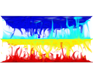
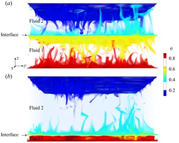
As shown in figure 1 for two 3-D cases and figure 2(a,b) for three 2-D cases, a large-scale circulation exists in each individual layer, which is consistent with previous two-layer studies (Davaille Reference Davaille1999; Xie & Xia Reference Xie and Xia2013; Liu et al. Reference Liu, Chong, Wang, Ng, Verzicco and Lohse2021a). From figure 2, we also observe that the temperature profile in each layer resembles that in the single-phase flow, namely the temperature remains constant in the bulk of each layer and strongly varies in the boundary layers near the plates and the interface.

Figure 1. Volume rendering of a snapshot of the thermal structures in two-layer RB convection in 3-D simulations at  $\mbox {Ra}=10^8$, $\mbox {We}=5$, the thermal conductivity coefficient ratio $\lambda _k=1$ and the thickness of the upper layer (a) $\alpha =0.5$ and (b) $\alpha =0.9$. The temperature field is colour-coded.

Figure 2. Snapshots of the 2-D simulations at  $\lambda _k=10$ and (a) $\alpha =0.19$, (b) $\alpha =0.81$ and (c) $\alpha =0.99$. The corresponding average (in time and space) temperature profiles are shown as blue (upper layer) and red (bottom layer) curves on panels (d–f), where the dashed lines denote the temperature at the interface.
When one layer becomes thin enough, we observe a temperature inversion therein (see figure 2b). A similar feature has been observed in Blass et al. (Reference Blass, Tabak, Verzicco, Stevens and Lohse2021), who considered sheared thermal convection, and in many prior papers (Belmonte, Tilgner & Libchaber Reference Belmonte, Tilgner and Libchaber1993; Tilgner, Belmonte & Libchaber Reference Tilgner, Belmonte and Libchaber1993; Ahlers et al. Reference Ahlers, Grossmann and Lohse2009). The reason for the inversion is that the fluctuations in the flow are not strong enough to fully mix the bulk. Then the remaining hot (cold) fluid is carried downward (upward) by the flow.
When one layer is sufficiently thin, pure thermal conduction instead of convection is observed. This is the case once the local  $\mbox {Ra}$ (defined with the layer thickness and its material parameters) becomes smaller than the onset value of convection. For example, in figure 2(c), the bottom layer has the local Rayleigh number $\mbox {Ra}_1=34.4$ and a pure conductive layer is found. Thus two regimes are identified: the regime with both convective layers appears at $0.04\le \alpha \le 0.96$; and the regime with one conductive layer and one convective layer at $\alpha \le 0.02$ or $\alpha \ge 0.98$. Since from figures 3(a), 4(b) and 4(c) we observe that heat flux $\mbox {Nu}$ and the interface temperature $\theta _i$ in the case of $\alpha =0.02$ and of $\alpha =0.04$ are very similar (the same for $\alpha =0.96$ and $\alpha =0.98$), we did not perform more cases in these transition zones of $0.02 < \alpha < 0.04$ and $0.96 < \alpha < 0.98$.

Figure 3. Global Nusselt number  $\mbox {Nu}$ normalized by $\mbox {Nu}_s$ of the single-phase system (pure fluid 1) as a function of (a) $\alpha$ and (b) $\lambda _k$ at $\mbox {Ra}=10^8$ and $\mbox {We}=5$. The symbols denote the numerical results and the lines the GL theory for two-layer system (3.1)–(3.4) at fixed (a) $\lambda _k=1$ and $10$ and (b) $\alpha =0.5$ and $0.99$, where the filled symbols/solid lines denote the regime with both convective layers, and the empty symbols/dashed lines the regime with one convective layer and one conductive layer. The 3-D cases are marked as cross symbols. The inset in (a) shows a zoom-in view for $\alpha$ close to $1$.
$1$.

Figure 4. Temperature at the interface  $\theta _i$ as function of $\alpha$. Panels (b,c) are zoom-in views of (a). The lines represent the GL theory for the two-layer system (black) in (3.1)–(3.4), and the approximate theory in (4.1)–(4.6) with $\mbox {Nu}$ versus $\mbox {Ra}$ scaling exponent of $\gamma =1/4$ (orange) and $\gamma =1/3$ (green). The symbols and line types are the same as in figure 3. The temperature distribution is not uniform on the interface. The error bar (i.e. the standard deviation of the temperature) for each case is smaller than the symbol size.
In the two distinct regimes, the heat transfer shows different  $\alpha$ dependence as shown in figure 3(a), where the heat flux is normalized with the heat flux $\mbox {Nu}_s$ for the single-phase flow (pure fluid 1). In the regime with both convective layers, the heat transfer hardly varies with $\alpha$ although the layer thickness $\alpha$ changes considerably. More specifically, we obtain $0.48\le \mbox {Nu}/\mbox {Nu}_s\le 0.57$ over $0.04\le \alpha \le 0.96$ for $\lambda _k=1$ while $1.00\le \mbox {Nu}/\mbox {Nu}_s\le 1.59$ for $\lambda _k=10$. In contrast, in the regime with one conductive layer, with $\alpha$ only increasing from $0.98$ to $1$,
$1$,  $\mbox {Nu}/\mbox {Nu}_s$ increases largely from $0.72$ to $1.00$ for $\lambda _k=1$ and from $1.72$ to $10.00$ for $\lambda _k=10$. Note that this interesting dependence of $\mbox {Nu}/\mbox {Nu}_s$ on $\alpha$ also holds for the 3-D cases.
Also the  $\lambda _k$ dependence is examined and shown in figure 3(b). As expected, the heat transfer in the two-layer system is limited by the layer with the lower thermal conductivity coefficient.
Obviously, in two-layer RB convection,  $\mbox {Nu}$ is affected by more parameters (namely $\alpha$ and the various ratios between the material properties such as $\lambda _k$) as compared with the single-phase case. To predict $\mbox {Nu}$ in the two-layer system, we regard the convection in each layer as single-phase convection. Then we apply the GL theory (Grossmann & Lohse Reference Grossmann and Lohse2000, Reference Grossmann and Lohse2001, Reference Grossmann and Lohse2002; Stevens et al. Reference Stevens, van der Poel, Grossmann and Lohse2013) in each individual layer,
 \begin{align} (\mbox{Nu}_j-1)\mbox{Ra}_j\mbox{Pr}_j^{{-}2}&=c_1\frac{\mbox{Re}_j^2}{g(\sqrt{\mbox{Re}_c/\mbox{Re}_j})}+c_2\mbox{Re}_j^3, \end{align}
 \begin{align} \mbox{Nu}_j-1&=c_3\mbox{Re}_j^{1/2}\mbox{Pr}_j^{1/2}\left\{f\left[\frac{2a\mbox{Nu}_j}{\sqrt{\mbox{Re}_c}}g\left(\sqrt{\frac{\mbox{Re}_c}{\mbox{Re}_j}}\right)\right]\right\}^{1/2} \nonumber\\ &\quad + c_4\mbox{Pr}_j\mbox{Re}_j f\left[\frac{2a\mbox{Nu}_j}{\sqrt{\mbox{Re}_c}}g\left(\sqrt{\frac{\mbox{Re}_c}{\mbox{Re}_j}}\right)\right], \end{align}
for  $j=1$ and $2$, indicating fluid $1$ and $2$, respectively. Here the local Rayleigh numbers in the respective layers are $\mbox {Ra}_1=(1-\alpha )^3 (1-\theta _i) \mbox {Ra}$ and $\mbox {Ra}_2=\alpha ^3 \theta _i \mbox {Ra}$ with $\theta _i$ being the temperature at the interface, and the local Prandtl numbers are $\mbox {Pr}_1=\nu _1/\kappa _1$ and $\mbox {Pr}_2=\nu _2/\kappa _2$. Here $f$ and $g$ are crossover functions, which are given by Grossmann & Lohse (Reference Grossmann and Lohse2000, Reference Grossmann and Lohse2001). We take the values of the parameters of the theory as given by Stevens et al. (Reference Stevens, van der Poel, Grossmann and Lohse2013), namely $c_1=8.05$, $c_2=1.38$, $c_3=0.487$, $c_4=0.0252$ and $\mbox {Re}_c=(2c_0)^2$ with $c_0=0.922$. These are based on various numerical and experimental data over a large range of $Ra$ and $Pr$ numbers. The above equations can be closed by imposing the heat flux balance at the interface,
 \begin{equation} Q_2=Q_1. \end{equation}
These heat fluxes are differently non-dimensionalized as Nusselt numbers, namely
 \begin{equation} \left. \begin{aligned} \mbox{Nu}_2 & =\frac{Q_2}{k_2\dfrac{\theta_i \varDelta}{\alpha H}},\\ \mbox{Nu}_1 & =\frac{Q_1}{k_1\dfrac{(1-\theta_i) \varDelta}{(1-\alpha)H}}. \end{aligned} \right\} \end{equation}
With (3.1)–(3.4) we obtain the GL-predictions for  $\mbox {Nu}(\mbox {Ra},\mbox {Pr})$ for the system with two convective layers.
Just as in single layer RB, the regime with one conductive layer has to be treated differently, instead of simply using (3.1) and (3.2). First, to determine the criteria for the occurrence, we use (3.1)–(3.4) to calculate  $\mbox {Ra}_1$ and $\mbox {Ra}_2$, and then compare them with the onset value of convection. Note that the conductive layer only occurs when the layer is thin enough, and in that case the aspect ratio of the conductive layer is much larger than $1$, allowing us to take the onset value to be $1708$ (Chandrasekhar Reference Chandrasekhar1981). Next, if one of the local Rayleigh numbers is smaller than $1708$, we use $\mbox {Nu}_j=1$ to replace (3.1) and (3.2). We get the critical layer thickness $\alpha _c=0.965$ for $\lambda _k=1$ ( $\alpha _c=0.972$ for $\lambda _k=10$) at $\mbox {Ra}_1=1708$ and $\alpha _c=0.035$ for $\lambda _k=1$ ( $\alpha _c=0.057$ for $\lambda _k=10$) at $Ra_2=1708$, which agree well with our simulations.
In figure 3, we compare  $\mbox {Nu}/\mbox {Nu}_s$ from the simulations with the predictions above. In both regimes, the dependence of $\mbox {Nu}/\mbox {Nu}_s$ on $\alpha$ and $\lambda _k$ agrees well with the predictions of the GL theory for the two-layer system. Note that no new fitting parameter was introduced at all.
The strong increase of the heat transfer for  $\alpha \le 0.02$ or $\alpha \ge 0.98$ can qualitatively be understood from the number of the conductive layers in the system. For $\alpha \le 0.02$ or $\alpha \ge 0.98$ there are only two conductive layers, namely at the top plate and at the bottom plate, and only one convective layer, which provides a thermal shortcut. In contrast, for $0.04\le \alpha \le 0.96$ there are two convective layers (with thermal shortcuts), but three conductive layers (namely, an addition one in between the two convective layers), and all three provide considerable thermal resistance, making the two layer system with two convective layers less heat conductive.
To further validate our quantitative predictions of the extended GL theory, we also compare the theoretical prediction with previous pioneering experiments by Wang et al. (Reference Wang, Mathai and Sun2019). These authors successfully created a closed system with highly efficient heat transfer enhancement by adding a minute concentration of heavy oil (HFE-7000) to RB convection of water. Via precise experimental measurements, two regimes could be identified: one is the boiling regime, where a significant heat transfer enhancement is observed and physically explained; and the other one is the non-boiling regime, which is a typical two-layer RB convection. The two layers are a water layer on the top and a heavy oil (HFE-7000) layer at the bottom. Based on the experiment settings of the pioneering work of Wang et al. (Reference Wang, Mathai and Sun2019), the parameters chosen here are  $\mbox {Ra}\approx 4.5\times 10^{10}$ and $\mbox {Pr}\approx 8.8$ (calculated for pure water) and $\lambda _\beta \approx 0.044$, $\lambda _\nu \approx 3.8$, $\lambda _\kappa \approx 3.3$ and $\lambda _k\approx 7.7$ (water over oil). In the system with $99\,\%$ water and $1\,\%$ oil in volume, Wang et al. (Reference Wang, Mathai and Sun2019) measured $\mbox {Nu}\approx 102$ (from figure 3e of that paper). With the extended GL theory for the two layers (3.1)–(3.4), we obtain a heat transfer $\mbox {Nu}=90.4$, which reasonably agrees with the experimental results.
4. Temperature at the interface
The mean temperature  $\theta _i$ (averaged in time and space) of the interface (the contour of $C=0.5$) plays a crucial role in the heat transfer of the two-layer system, since it determines the value of the local Rayleigh numbers as mentioned in § 3. We plot the $\alpha$ dependence of $\theta _i$ in figure 4. Similarly to the $\alpha$ dependence of $\mbox {Nu}/\mbox {Nu}_s$, we again observe that $\theta _i$ is insensitive to the change in $\alpha$ over $0.04\le \alpha \le 0.96$, whereas significant changes in $\theta _i$ are observed for $\alpha \le 0.02$ or $\alpha \ge 0.98$.
To explain this  $\alpha$ dependence of the mean temperature $\theta _i$ of the interface, we again use the GL theory to estimate $\mbox {Nu}(Ra,Pr)$ in each of the two layers and then plug the results into (3.4) to obtain $\theta _i(\alpha,\lambda _k)$. The results are shown as black lines in figure 4 (for the $\theta _i(\alpha )$ dependence) and figure 5 (for the $\theta _i(\lambda _k)$ dependence), where the GL-predictions for the interfacial temperature $\theta _i(\alpha,\lambda _k)$ agree very well with the numerical results, demonstrating once more the predictive power of the GL theory.

Figure 5. Temperature at the interface  $\theta _i$ as function of $\lambda _k$. The lines represent the full GL theory for the two-layer system (black) in (3.1)–(3.4) and the approximate theory in (4.3) and (4.5) with $\mbox {Nu}$ versus $\mbox {Ra}$ scaling exponent of $\gamma =1/4$ (red) and $\gamma =1/3$ (blue). All the cases here are 2-D cases. The symbols and line types are the same as in figure 3.
The strong decrease (increase) of the interfacial temperature  $\theta _i$ for small $\alpha \le 0.02$ (large $\alpha \ge 0.98$) in figure 4 can straightforwardly be understood by the proximity of the interface to the cold (hot) plate and our above explanations of the $\alpha$-dependence of $\mbox {Nu}$. The $\lambda _k$-dependence of $\theta _i$ in figure 5 can qualitatively be understood as follows. To ensure the heat flux conservation at the interface, for large $\lambda _k>1$ (namely, larger thermal conductivity of the fluid in the top layer than in the bottom one) the temperature difference between the interface and the cold top plate ( $\theta _i-0$) must be smaller. This argument also implies a decrease of the interfacial temperature $\theta _i$ with increasing $\lambda _k$.
For the above-mentioned case of Wang et al. (Reference Wang, Mathai and Sun2019) for the water–heavy-oil two-layer RB convection, our theory gives a mean interface temperature  $\theta _i=0.53$, i.e. slightly enhanced as compared with the case $\theta _i=1/2$, which would occur if the material properties of the two layers were identical. This slight increase reflects that $\kappa _1<\kappa _2$, and that consequently the bottom thermal BL is thinner than the top one, leading to a better thermal coupling of the centre interface to the hot bottom plate as compared with the cold top one, similarly as in non-Oberbeck–Boussinesq thermal convection with water (Ahlers et al. Reference Ahlers, Brown, Fontenele Araujo, Funfschilling, Grossmann and Lohse2006), where the hot bottom thermal BL is also thinner than the cold top one and the mean bulk temperature enhanced. Note that in their experiments, Wang et al. (Reference Wang, Mathai and Sun2019) could not provide experimental data for the interface temperature, as this would experimentally be too challenging; so here we cannot compare with experiment.
To obtain a simple relationship for  $\theta _i(\alpha,\lambda _k)$, rather than using the full GL theory, an abbreviated approach is to just use an effective scaling exponent $\gamma$ to approximate the full GL theory, ignoring the crossovers between the regimes,
 \begin{equation} \mbox{Nu}_j\sim\mbox{Ra}^\gamma_j, \end{equation}
where  $\gamma$ and the prefactor are constant when $\mbox {Ra}$ varies over a small range.
Then, by applying (4.1) in each layer and imposing the heat flux balance at the interface (3.3) and (3.4), we obtain
 \begin{equation} [(1-\alpha)^3(1-\theta_i)\mbox{Ra}]^\gamma k_1\frac{(1-\theta_i)\varDelta}{(1-\alpha)H} = (\alpha^3 \theta_i \mbox{Ra})^\gamma k_2 \frac{\theta_i \varDelta}{\alpha H}. \end{equation}
Note that the prefactor of (4.1) cancels out. After rewriting equation (4.2), we get the following approximate scaling law for the regime with two convective layers:
 \begin{equation} \frac{1}{\theta_i}-1 = \lambda_k^{{1}/({1+\gamma})}\,\left(\frac{1}{\alpha}-1\right)^{({1-3\gamma})/({1+\gamma})}. \end{equation}
We now consider the value of  $\gamma$ to vary between $1/4$ and $1/3$, which is reasonable for the classical regime of RB convection (Ahlers et al. Reference Ahlers, Grossmann and Lohse2009; Lohse & Xia Reference Lohse and Xia2010; Chillà & Schumacher Reference Chillà and Schumacher2012; Shishkina Reference Shishkina2021). Correspondingly, the exponent $(1-3\gamma )/(1+\gamma )$ in (4.3) varies from $0.2$ to $0$. This low value reflects the relatively weak $\alpha$ dependence of $\theta _i$ for the regime with two convective layers.
To validate the simplified relationship (4.3), we show the results for  $\gamma =1/4$ and $1/3$ in figure 4(a) and figure 5. In both figures, the numerical data and the full GL predictions are in-between the simple relationship of (4.3) with $\gamma =1/4$ and that one with $\gamma =1/3$, since a constant effective exponent $\gamma$ is appropriately only within a small range of $\mbox {Ra}$ while the full GL theory well describes a wide range of $\mbox {Ra}$.
For the cases with the lower layer being thin enough to be purely conductive (i.e.  $\alpha \to 1$), we must use $\mbox {Nu}_1=1$ in the lower layer together with (4.1) for the upper layer, which gives
 \begin{equation} k_1\frac{(1-\theta_i)\varDelta}{(1-\alpha)H}\sim(\alpha^3 \theta_i \mbox{Ra})^\gamma k_2 \frac{\theta_i \varDelta}{\alpha H}. \end{equation}
Then, by rewriting this equation, we obtain
 \begin{equation} \frac{1-\theta_i}{\theta_i^{(1+\gamma)}} \sim \lambda_k \,\alpha^{3\gamma-1}(1-\alpha). \end{equation}
Although the term  $\alpha ^{3\gamma -1}$ has only weak $\alpha$ dependence (considering $\gamma$ to be between $1/4$ and $1/3$), $\theta _i$ is sensitive to $\alpha$ because of the term $1-\alpha$. We obtain the prefactor in (4.5) by matching (4.5) and (4.3) at $\mbox {Ra}_1=1708$, since (4.5) is applicable for $\mbox {Ra}_1 \le 1708$ and (4.3) for $\mbox {Ra}_1 \ge 1708$.
Similarly, in the case when the upper layer is purely conductive ( $\alpha \to 0$), we obtain
 \begin{equation} \frac{\theta_i}{(1-\theta_i)^{1+\gamma}} \sim \lambda_k \,(1-\alpha)^{3\gamma-1}\alpha, \end{equation}
which also indicates that  $\theta _i$ is sensitive to $\alpha$ in that regime. Furthermore, (4.3)–(4.6) show that $\theta _i$ is sensitive to $\lambda _k$ in all the situations.
Also for these regimes with  $\alpha \le 0.02$ or $\alpha \ge 0.98$ we validate the derived approximate relations (4.5) and (4.6) using $\gamma =1/4$ and $\gamma =1/3$ in figures 4(b), 4(c) and 5. Again, good agreements are achieved also in these regimes with one conductive layer and one convective layer.
5. Effects of the deformable interface
In RB convection with two layers, the large-scale circulations are confined within each layer provided that the surface tension is strong enough, i.e.  $\mbox {We}$ small enough. For example, for $\mbox {We}=5$ as in our simulations, the interface only deforms slightly as can be seen in figures 1 and 2. However, on increasing $\mbox {We}$, the interface becomes wavy (see figure 6a) and even breaks up (see figure 6b). We have derived the criterion for interface breakup in our previous study (Liu et al. Reference Liu, Chong, Wang, Ng, Verzicco and Lohse2021a).

Figure 6. (a) Snapshots with the wavy interface at  $\mbox {We}=20$ and (b) with the breakup interface at $\mbox {We}=2000$. (c) Corresponding average temperature profiles. (d) Here $\mbox {Nu}/\mbox {Nu}_s$ as a function of $\mbox {We}$. The lines represent the extended GL theory for the two-layer system, ignoring the interface dynamics. All the cases here are 2-D cases at fixed $\mbox {Ra}=10^8$, $\alpha =0.5$ and $\lambda _k=1$.
In the wavy case, the large-scale circulation still exists in each layer. In contrast, in the breakup case, the surface tension is too weak and stirring of the fluid layers takes place as evidenced by the vanishing of the sharp temperature jump in the middle of the cell in figure 6(c).
The Nusselt number also exhibits a highly non-trivial  $\mbox {We}$ dependence, in accordance with the quite different flow dynamics. When the interface remains intact, the values of $\mbox {Nu}/\mbox {Nu}_s$ are close to the prediction from the extended GL theory for the two-layer system. When there is a wavy interface, $\mbox {Nu}/\mbox {Nu}_s$ becomes slightly larger than the GL prediction. However, when the interface breaks up, $\mbox {Nu}/\mbox {Nu}_s$ directly jumps to a saturated value, which is slightly smaller than the value obtained for single-phase flow of the better conducting layer. The reason for the slight difference to the single phase RB case is that although a clear two-layer structure has been washed out, the existence of the heavy droplets of fluid 1 and the light ones of fluid 2 will anyhow slow down the convective flow, hindering the heat flux.
6. Conclusions and outlook
Turbulent RB convection with two immiscible fluid layers is numerically investigated for various layer thicknesses ( $0.01\le \alpha \le 0.99$) and thermal conductivity coefficient ratios ( $1\le \lambda _k\le 10$) both in two dimensions and three dimensions. Two regimes can be identified: in regime 1, two convective layers appear; while in regime 2, one layer is sufficiently thin and dominated by pure conduction because the local $\mbox {Ra}$ thereof is smaller than the onset value of convection. The heat transfer $\mbox {Nu}$ is sensitive to the layer thickness $\alpha$ in regime 2 but not in regime 1. To explain the observed $\mbox {Nu}$ behaviours, we extend the GL theory of single-phase RB convection to the two-layer system. The predictions from the extended GL theory for the overall heat transport agree well with the simulations for various $\lambda _k$ and also with experimental data. Moreover, the temperature at the interface can also be predicted nicely for the two-layer system. We further derived a simple scaling model to explicitly show the relationship between $\theta _i$, $\alpha$ and $\lambda _k$. Finally, the effect of the deformable interface on the heat transfer is studied, where we find that the extended GL theory for the two-layer system still roughly holds, as long as the interface does not break up.
This study showed that the extended GL theory for the two-layer system works for various ratios of the thermal conductivity coefficient in two layers, which is a key property among all material properties, but we expect that the theory also holds when we vary the ratio of other properties, e.g. the thermal expansion coefficient, the density, the dynamic viscosity, the thermal diffusivity (as had already been done in the pioneering experiment of Wang et al. (Reference Wang, Mathai and Sun2019)) and the specific heat capacity. The ratios of all properties can be represented by the local dimensionless numbers  $\mbox {Ra}_1$, $\mbox {Ra}_2$, $\mbox {Pr}_1$ and $\mbox {Pr}_2$ in the extended GL theory. It would be also interesting to test this theory for various other global $\mbox {Ra}$ and $\mbox {Pr}$, which here were fixed at $\mbox {Ra}=10^8$ and $\mbox {Pr}=4.38$.
The results in this work can find many realistic applications, such as in atmospheric oceanography, geophysics and industry. Our main finding, the layer thickness dependence of heat transport in the two-layer system, also suggests that the two-layer system is not a good choice if one wants to enhance the overall heat transfer. When the two-layer system is unavoidable anyhow, to ensure the maximal heat transfer, the layer with the lower thermal conductivity coefficient must be kept thin enough to ensure that pure conduction occurs in this layer, which then is identical to the thermal boundary layer at the corresponding plate. For thicker liquid layers the heat transfer has to overcome three conductive layers, namely the two at the plates and one extra one between the two convective layers, and the thermal resistance is correspondingly larger and the overall heat transfer lower.
Acknowledgments
We acknowledge PRACE for awarding us access to MareNostrum in Spain at the Barcelona Computing Center (BSC) under the project nos.  $2020225335$ and $2020235589$. K.L.C. acknowledges the Shanghai Science and Technology Program under project no. 19JC1412802. This work was also carried out on NWO Domain Science for the use of the national computer facilities.
Funding
The work was financially supported by an ERC-Advanced Grant under the project no.  $740479$ and the NWO Max Planck Centre ‘Complex Fluid Dynamics’.
Declaration of interests
The authors report no conflict of interest.


 Open access