





1. Introduction
Turbulence can significantly intensify or inhibit particle settling with respect to the terminal velocity in quiescent fluid, $W_0$
. Already Maxey (Reference Maxey1987) theorised that spherical particles with a diameter
$W_0$
. Already Maxey (Reference Maxey1987) theorised that spherical particles with a diameter $d_p$
smaller than the Kolmogorov scale
$d_p$
smaller than the Kolmogorov scale $\eta$
would settle faster in turbulence than in still fluid, being preferentially swept in regions of high strain and downward velocity fluctuations. This picture was supported in numerous numerical studies, such as Wang & Maxey (Reference Wang and Maxey1993), Bosse, Kleiser & Meiburg (Reference Bosse, Kleiser and Meiburg2006), Dejoan & Monchaux (Reference Dejoan and Monchaux2013), Bec, Homann & Ray (Reference Bec, Homann and Ray2014), Rosa et al. (Reference Rosa, Parishani, Ayala and Wang2016), Frankel et al. (Reference Frankel, Pouransari, Coletti and Mani2016), Ireland, Bragg & Collins (Reference Ireland, Bragg and Collins2016), Baker et al. (Reference Baker, Frankel, Mani and Coletti2017), Tom & Bragg (Reference Tom and Bragg2019), among others, in which the fluid flow was resolved by direct numerical simulation and the dispersed phase was predicted using the point-particle approach.
$\eta$
would settle faster in turbulence than in still fluid, being preferentially swept in regions of high strain and downward velocity fluctuations. This picture was supported in numerous numerical studies, such as Wang & Maxey (Reference Wang and Maxey1993), Bosse, Kleiser & Meiburg (Reference Bosse, Kleiser and Meiburg2006), Dejoan & Monchaux (Reference Dejoan and Monchaux2013), Bec, Homann & Ray (Reference Bec, Homann and Ray2014), Rosa et al. (Reference Rosa, Parishani, Ayala and Wang2016), Frankel et al. (Reference Frankel, Pouransari, Coletti and Mani2016), Ireland, Bragg & Collins (Reference Ireland, Bragg and Collins2016), Baker et al. (Reference Baker, Frankel, Mani and Coletti2017), Tom & Bragg (Reference Tom and Bragg2019), among others, in which the fluid flow was resolved by direct numerical simulation and the dispersed phase was predicted using the point-particle approach.
Enhanced settling of particles in turbulent air was observed in laboratory experiments for the first time by Aliseda et al. (Reference Aliseda, Cartellier, Hainaux and Lasheras2002) and later by several others, including Yang & Shy (Reference Yang and Shy2005) and Good et al. (Reference Good, Ireland, Bewley, Bodenschatz, Collins and Warhaft2014), as well as in field measurements of snowfall by Nemes et al. (Reference Nemes, Dasari, Hong, Guala and Coletti2017) and Li et al. (Reference Li, Lim, Berk, Abraham, Heisel, Guala, Coletti and Hong2021). It was not until Petersen, Baker & Coletti (Reference Petersen, Baker and Coletti2019) and Berk & Coletti (Reference Berk and Coletti2021), however, that the preferential sweeping mechanism was directly observed in a fully turbulent flow. Bergougnoux et al. (Reference Bergougnoux, Bouchet, Lopez and Guazzelli2014) also clearly demonstrated it in a cellular flow at low Reynolds numbers. It was argued that such an effect is prevalent when particles have a Stokes number $ \textit{St}_\eta = \tau _p/\tau _\eta$
of order one (where
$ \textit{St}_\eta = \tau _p/\tau _\eta$
of order one (where $\tau _\eta$
is the Kolmogorov time scale), since these particles couple most effectively to the smallest eddies. The effect was observed to be dramatic, more than doubling the settling velocities compared with still-fluid conditions. Nevertheless, experimental studies on particles in turbulent water over comparable ranges of
$\tau _\eta$
is the Kolmogorov time scale), since these particles couple most effectively to the smallest eddies. The effect was observed to be dramatic, more than doubling the settling velocities compared with still-fluid conditions. Nevertheless, experimental studies on particles in turbulent water over comparable ranges of $ \textit{St}_\eta$
usually report hindered settling (Kawanisi & Shiozaki Reference Kawanisi and Shiozaki2008; Zhou & Cheng Reference Zhou and Cheng2009; Akutina et al. Reference Akutina, Revil-Baudard, Chauchat and Eiff2020). The specific effect of the particle-to-fluid density ratio
$ \textit{St}_\eta$
usually report hindered settling (Kawanisi & Shiozaki Reference Kawanisi and Shiozaki2008; Zhou & Cheng Reference Zhou and Cheng2009; Akutina et al. Reference Akutina, Revil-Baudard, Chauchat and Eiff2020). The specific effect of the particle-to-fluid density ratio $\tilde \rho =\rho _p/\rho _{\kern-1pt f}$
, however, has not been directly investigated. In general, the magnitude and direction of the settling velocity, even in the seemingly simple case of homogeneous turbulence, remain unclear.
$\tilde \rho =\rho _p/\rho _{\kern-1pt f}$
, however, has not been directly investigated. In general, the magnitude and direction of the settling velocity, even in the seemingly simple case of homogeneous turbulence, remain unclear.
This state of affair may be partly rooted in other effects of turbulence which, unlike preferential sweeping, are expected to reduce the settling velocity. As summarised by Nielsen (Reference Nielsen1993), these include: vortex trapping (weakly inertial particles trapped in vortices), loitering (particles dwelling in the upward side of turbulent eddies) and drag nonlinearity (the net increase of drag force induced by fluctuations of the particle–fluid relative velocity, when the particle Reynolds number is significant). The competition of different mechanisms makes the net effect on the settling rate sensitive to the specific parameters, including the settling velocity ratio, $Sv_L=W_0/u_{\textit{rms}}$
, where
$Sv_L=W_0/u_{\textit{rms}}$
, where $u_{\textit{rms}}$
is the root mean square (r.m.s.) of the fluid velocity fluctuations. This is also termed Rouse number (Dejoan & Monchaux Reference Dejoan and Monchaux2013; Ferran et al. Reference Ferran, Machicoane, Aliseda and Obligado2023) and its inverse is sometimes referred to as turbulence intensity (Fornari et al. Reference Fornari, Picano, Sardina and Brandt2016b
). Some authors rather report
$u_{\textit{rms}}$
is the root mean square (r.m.s.) of the fluid velocity fluctuations. This is also termed Rouse number (Dejoan & Monchaux Reference Dejoan and Monchaux2013; Ferran et al. Reference Ferran, Machicoane, Aliseda and Obligado2023) and its inverse is sometimes referred to as turbulence intensity (Fornari et al. Reference Fornari, Picano, Sardina and Brandt2016b
). Some authors rather report $Sv_\eta = W_0/u_\eta$
, where
$Sv_\eta = W_0/u_\eta$
, where $u_\eta \sim u_{\textit{rms}}Re_L^{-1/4}$
is the Kolmogorov velocity,
$u_\eta \sim u_{\textit{rms}}Re_L^{-1/4}$
is the Kolmogorov velocity, $ \textit{Re}_L = u_{\textit{rms}}L/\nu$
is the Reynolds number based on the integral scale
$ \textit{Re}_L = u_{\textit{rms}}L/\nu$
is the Reynolds number based on the integral scale $L$
and
$L$
and $\nu$
is the fluid kinematic viscosity.
$\nu$
is the fluid kinematic viscosity.
Likely, the variability in experimental results is also the consequence of challenges in constructing and characterising laboratory systems. For example, when measuring the particle settling velocity in advective flows such as wind or water tunnels, significant biases can ensue from uncertainty in measuring fall speeds much smaller than the mean velocity (Good, Gerashchenko & Warhaft Reference Good, Gerashchenko and Warhaft2012). Closed systems such as chambers with oscillating grids may also induce substantial recirculation (Blum et al. Reference Blum, Kunwar, Johnson and Voth2010), in turn affecting the settling (Zhou & Cheng Reference Zhou and Cheng2009). The ideal configuration requires measuring with high accuracy the fall speed of well-characterised particles settling in steady, homogeneous turbulence with negligible mean velocity and shear/strain. Additionally, the homogeneous region should stretch over a portion of space large enough to allow for the turbulent cascade to develop without the influence of boundaries (Carter et al. Reference Carter, Petersen, Amili and Coletti2016) and for the particles to respond to the turbulence and reach terminal velocity in it (Petersen et al. Reference Petersen, Baker and Coletti2019).
(a) Normalised settling velocity as a function of $Sv_L$
, from previous experiments (Aliseda et al. Reference Aliseda, Cartellier, Hainaux and Lasheras2002; Yang & Shy Reference Yang and Shy2005; Good et al. Reference Good, Ireland, Bewley, Bodenschatz, Collins and Warhaft2014; Berk & Coletti Reference Berk and Coletti2021) and simulations (Wang & Maxey Reference Wang and Maxey1993; Yang & Lei Reference Yang and Lei1998; Dejoan & Monchaux Reference Dejoan and Monchaux2013; Good et al. Reference Good, Ireland, Bewley, Bodenschatz, Collins and Warhaft2014; Rosa et al. Reference Rosa, Parishani, Ayala and Wang2016; Ireland et al. Reference Ireland, Bragg and Collins2016). (b) Cases investigated in the present study, spanning a wide range of
$Sv_L$
, from previous experiments (Aliseda et al. Reference Aliseda, Cartellier, Hainaux and Lasheras2002; Yang & Shy Reference Yang and Shy2005; Good et al. Reference Good, Ireland, Bewley, Bodenschatz, Collins and Warhaft2014; Berk & Coletti Reference Berk and Coletti2021) and simulations (Wang & Maxey Reference Wang and Maxey1993; Yang & Lei Reference Yang and Lei1998; Dejoan & Monchaux Reference Dejoan and Monchaux2013; Good et al. Reference Good, Ireland, Bewley, Bodenschatz, Collins and Warhaft2014; Rosa et al. Reference Rosa, Parishani, Ayala and Wang2016; Ireland et al. Reference Ireland, Bragg and Collins2016). (b) Cases investigated in the present study, spanning a wide range of $\tilde \rho$
and plotted in the
$\tilde \rho$
and plotted in the $ \textit{St}_\eta {-}Sv_\eta$
space.
$ \textit{St}_\eta {-}Sv_\eta$
space.
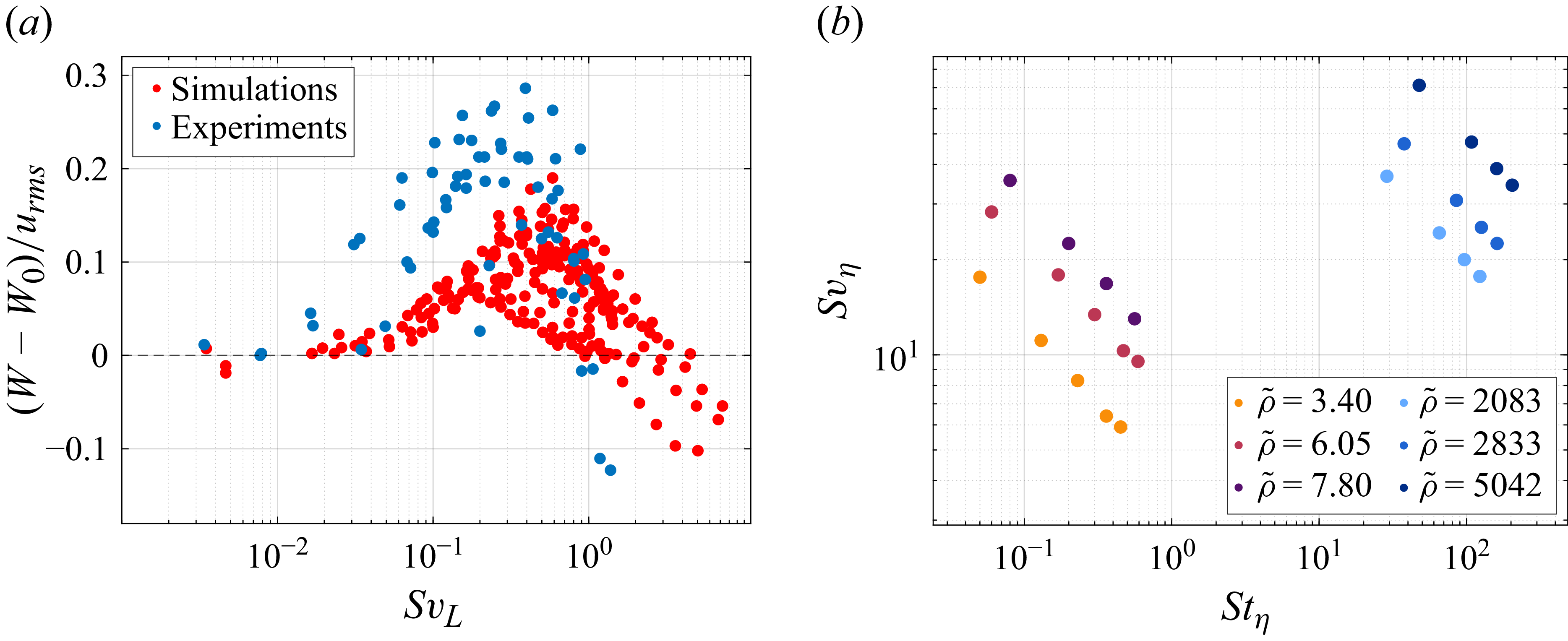
Figure 1. Long description
Panel A: A scatter plot shows the normalized settling velocity as a function of the Stokes number. The x-axis is labeled S v L and spans from 10^−2 to 10^1. The y-axis is labeled (W-W0)/u rms and ranges from −0.1 to 0.3. Red dots represent simulation data, while blue dots represent experimental data. The plot shows a trend where the normalized settling velocity increases with S v L up to a certain point and then decreases. Panel B: Another scatter plot illustrates cases investigated in the present study, spanning a wide range of parameters. The x-axis is labeled S t η and ranges from 10^−1 to 10^2. The y-axis is labeled S v η and ranges from 10^0 to 10^2. Different colors represent different density ratios, with a legend indicating values from 3.40 to 6050.
Numerical simulations face their own difficulties. The point-particle approximation, necessary to model high-Reynolds number regimes with realistically large numbers of particles, has well-known limitations (Eaton Reference Eaton2009; Brandt & Coletti Reference Brandt and Coletti2022), though partly alleviated by advanced methods to estimate the fluid velocity at the particle location (Gualtieri et al. Reference Gualtieri, Sardina, Picano and Casciola2015; Horowitz & Mani Reference Horowitz and Mani2016; Ireland & Desjardins Reference Ireland and Desjardins2017). The particle equation of motion (Maxey & Riley Reference Maxey and Riley1983; Gatignol Reference Gatignol1983) assumes superposition of forces strictly applicable only in the low-Reynolds number regime (Brandt & Coletti Reference Brandt and Coletti2022) and includes terms not trivial to calculate such as the Basset-history force (Haller Reference Haller2019). Simulations conducted in the same range of parameters disagree particularly on the role of nonlinear drag: Good et al. (Reference Good, Ireland, Bewley, Bodenschatz, Collins and Warhaft2014) found it to cause significant settling reduction, while such an effect was negligible as noted by Rosa et al. (Reference Rosa, Parishani, Ayala and Wang2016) possibly due to different forcing schemes. Interface-resolved simulations are, in principle, able to capture all relevant particle–turbulence interactions and have contributed invaluably to our understanding of them; see, among many others, Tenneti & Subramaniam (Reference Tenneti and Subramaniam2014), Uhlmann & Chouippe (Reference Uhlmann and Chouippe2017), Schneiders, Meinke & Schröder (Reference Schneiders, Meinke and Schröder2017), Mehrabadi et al. (Reference Mehrabadi, Horowitz, Subramaniam and Mani2018), Peng, Sun & Wang (Reference Peng, Sun and Wang2023), Balachandar, Peng & Wang (Reference Balachandar, Peng and Wang2024), Chiarini & Rosti (Reference Chiarini and Rosti2024). Most such studies in homogeneous turbulence, however, neglected gravitational settling, with the exception of Fornari et al. (Reference Fornari, Picano and Brandt2016a ,Reference Fornari, Picano, Sardina and Brandt b ), Chouippe & Uhlmann (Reference Chouippe and Uhlmann2019) and Peng et al. (Reference Peng, Karzhaubayev, Wang, Chen and Niu2025). Also, most studies of this type simulated particles much larger than the Kolmogorov scale (except Chiarini, Tandurella & Rosti Reference Chiarini, Tandurella and Rosti2025, who however did not consider gravity) for which the flow modification by geometric effects and wakes leads to fundamentally different dynamics (Brandt & Coletti Reference Brandt and Coletti2022).
In summary, the complexity of the process, along with challenges in setting up laboratory experiments and numerical simulations, has resulted in a lack of consensus on the magnitude and even the direction of settling modification for small particles in turbulence. This is illustrated in figure 1(a), which plots the normalised change in settling velocity $(W-W_0)/u_{\textit{rms}}$
as a function of
$(W-W_0)/u_{\textit{rms}}$
as a function of $Sv_L$
, for a number of previous experiments and numerical studies focused on the case
$Sv_L$
, for a number of previous experiments and numerical studies focused on the case $d_p \lesssim \eta$
. (Here and in the following, the vertical velocity
$d_p \lesssim \eta$
. (Here and in the following, the vertical velocity $W$
is taken positive when downward.) The large discrepancies limit our predictive ability and thwart the mechanistic understanding of the phenomenon, leaving the following fundamental questions unanswered. What parameters determine the direction and magnitude of settling rate modification? Why does turbulence seem to affect particle settling velocity differently in air and water? Which mechanisms influencing the settling velocity prevail in different conditions?
$W$
is taken positive when downward.) The large discrepancies limit our predictive ability and thwart the mechanistic understanding of the phenomenon, leaving the following fundamental questions unanswered. What parameters determine the direction and magnitude of settling rate modification? Why does turbulence seem to affect particle settling velocity differently in air and water? Which mechanisms influencing the settling velocity prevail in different conditions?
In an effort to address these questions, we present the results of an extensive measurement campaign in which solid particles with $d_p = O(\eta )$
settle in homogeneous turbulence. We leverage two different large-scale, zero-mean-flow turbulence chambers, operating with water and air, respectively. This allows us to investigate the effect of the density ratio and to span a wide range of
$d_p = O(\eta )$
settle in homogeneous turbulence. We leverage two different large-scale, zero-mean-flow turbulence chambers, operating with water and air, respectively. This allows us to investigate the effect of the density ratio and to span a wide range of $ \textit{St}_\eta$
and
$ \textit{St}_\eta$
and $Sv_\eta$
, as is illustrated in figure 1(b). We find that, irrespective of
$Sv_\eta$
, as is illustrated in figure 1(b). We find that, irrespective of $\tilde \rho$
, the large scales are crucial as signalled by the decisive role of
$\tilde \rho$
, the large scales are crucial as signalled by the decisive role of $Sv_L$
, and quantify the relative magnitude of loitering and nonlinear drag in hindering the settling velocity. The paper is organised as follows: in § 2, we describe the experimental apparatus and methodology; in § 3, we report the settling rate for the various cases and discuss the mechanisms by which turbulence modifies it; finally, we discuss the results and draw conclusions in § 4.
$Sv_L$
, and quantify the relative magnitude of loitering and nonlinear drag in hindering the settling velocity. The paper is organised as follows: in § 2, we describe the experimental apparatus and methodology; in § 3, we report the settling rate for the various cases and discuss the mechanisms by which turbulence modifies it; finally, we discuss the results and draw conclusions in § 4.
2. Methodology
2.1. Experimental procedure
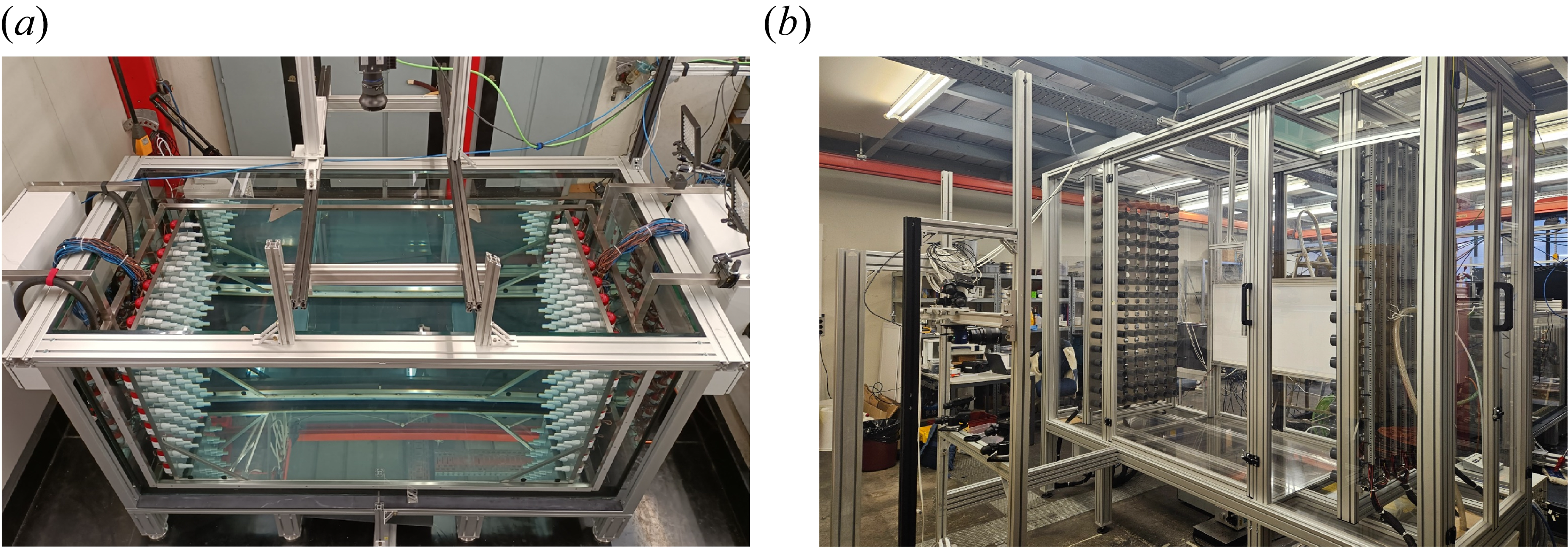
The experiments are conducted in two zero-mean flow chambers, depicted in figures 2(a) and 2(b). Both of them feature two facing arrays of jets firing in random sequence to generate homogeneous turbulence. The water chamber was introduced and characterised in detail by Ruth & Coletti (Reference Ruth and Coletti2024), Li et al. (Reference Li, Wang, Qi and Coletti2024) and Qi, Li & Coletti (Reference Qi, Li and Coletti2025); while the air chamber is very similar to the one introduced by Carter et al. (Reference Carter, Petersen, Amili and Coletti2016), qualified in detail by Carter & Coletti (Reference Carter and Coletti2017, Reference Carter, Petersen, Amili and Coletti2018) and used to study particle-laden air turbulence by Petersen et al. (Reference Petersen, Baker and Coletti2019), Berk & Coletti (Reference Berk and Coletti2021), Hassaini & Coletti (Reference Hassaini and Coletti2022) and Hassaini, Petersen & Coletti (Reference Hassaini, Petersen and Coletti2023). Therefore, the apparatuses and measurement techniques are only briefly described here. The water chamber has dimensions of $2\,\times \,1\,\times \,1\,\mathrm{m}^3$
and features two
$2\,\times \,1\,\times \,1\,\mathrm{m}^3$
and features two $8\,\times \,8$
arrays of pumps controlled by programmable logic circuits (PLCs), firing jets whose mass flow rate is adjusted by a pulse-width-modulation scheme, in turn setting
$8\,\times \,8$
arrays of pumps controlled by programmable logic circuits (PLCs), firing jets whose mass flow rate is adjusted by a pulse-width-modulation scheme, in turn setting $u_{\textit{rms}}$
. The air chamber has dimensions of
$u_{\textit{rms}}$
. The air chamber has dimensions of $3\,\times \,2.1\,\times \,1.1\,\mathrm{m}^3$
and features two
$3\,\times \,2.1\,\times \,1.1\,\mathrm{m}^3$
and features two $16\,\times \,8$
arrays of quasi-synthetic jets fired by PLC-controlled solenoid valves, the mass flow rate of the jets being controlled by the pressure in the manifold framing each array. In both systems, the jets actuation follows the sunbathing algorithm proposed by Variano & Cowen (Reference Variano and Cowen2008), with mean firing times of
$16\,\times \,8$
arrays of quasi-synthetic jets fired by PLC-controlled solenoid valves, the mass flow rate of the jets being controlled by the pressure in the manifold framing each array. In both systems, the jets actuation follows the sunbathing algorithm proposed by Variano & Cowen (Reference Variano and Cowen2008), with mean firing times of $3\,\mathrm{s}$
and
$3\,\mathrm{s}$
and $0.5\,\mathrm{s}$
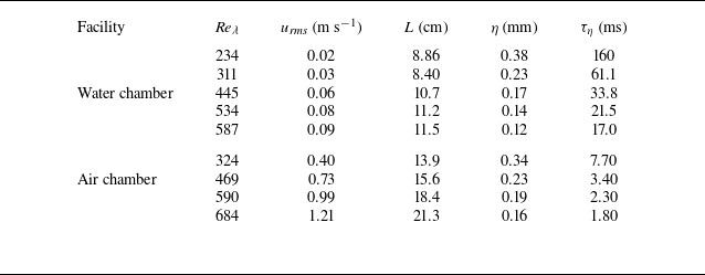
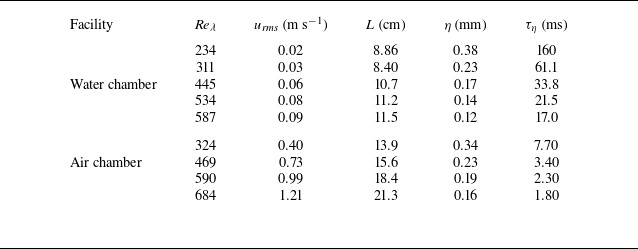
for the water and air chamber, respectively. The jets generate homogeneous turbulence in a central region substantially larger than the integral length scale of the turbulence, whose properties are summarised in table 1. The considered range of Taylor-microscale Reynolds number,
$0.5\,\mathrm{s}$
for the water and air chamber, respectively. The jets generate homogeneous turbulence in a central region substantially larger than the integral length scale of the turbulence, whose properties are summarised in table 1. The considered range of Taylor-microscale Reynolds number, $ \textit{Re}_\lambda$
, allows for the development of an inertial sub-range where Kolmogorov’s (Reference Kolmogorov1941) scaling applies. The mean flow is much smaller than the velocity fluctuations (and, importantly, negligibly small in the vertical direction) and there is no sizeable mean shear.
$ \textit{Re}_\lambda$
, allows for the development of an inertial sub-range where Kolmogorov’s (Reference Kolmogorov1941) scaling applies. The mean flow is much smaller than the velocity fluctuations (and, importantly, negligibly small in the vertical direction) and there is no sizeable mean shear.
The two zero-mean-flow turbulence chambers used in this study, featuring facing arrays of randomly actuated jets with (a) water and (b) air as working fluid.
Main properties of the homogeneous turbulence generated in the two experimental installations.
Particles are introduced in both chambers through a system of sieves agitated by an electro-mechanical shaker, whose frequency controls the mass flux and therefore the solid volume fraction. This is kept below $10^{-5}$
in water and below
$10^{-5}$
in water and below $10^{-7}$
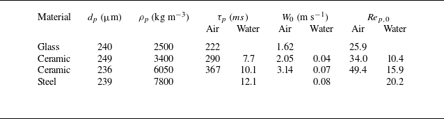
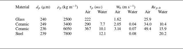
in air, minimising two-way coupling with the turbulence and four-way coupling between particles (Brandt & Coletti Reference Brandt and Coletti2022). Four types of size-selected particles are used, made of steel, ceramic and glass (see properties in table 2) with a high level of sphericity as verified by microscopy. The particles are only weakly poly-dispersed, with standard deviations of their diameter below 20 % of the mean. Their response time is calculated using the Schiller–Naumann correlation (Clift, Grace & Weber Reference Clift, Grace and Weber2005) and accounting for added mass effects (Ling, Parmar & Balachandar Reference Ling, Parmar and Balachandar2013),
$10^{-7}$
in air, minimising two-way coupling with the turbulence and four-way coupling between particles (Brandt & Coletti Reference Brandt and Coletti2022). Four types of size-selected particles are used, made of steel, ceramic and glass (see properties in table 2) with a high level of sphericity as verified by microscopy. The particles are only weakly poly-dispersed, with standard deviations of their diameter below 20 % of the mean. Their response time is calculated using the Schiller–Naumann correlation (Clift, Grace & Weber Reference Clift, Grace and Weber2005) and accounting for added mass effects (Ling, Parmar & Balachandar Reference Ling, Parmar and Balachandar2013), $\tau _p = d_p^2/[12\nu \beta (1+0.15Re_{p,0}^{0.687})]$
, where
$\tau _p = d_p^2/[12\nu \beta (1+0.15Re_{p,0}^{0.687})]$
, where $\beta =3/(2\tilde \rho +1)$
and
$\beta =3/(2\tilde \rho +1)$
and $ \textit{Re}_{p,0}$
is the particle Reynolds number. The latter is taken as
$ \textit{Re}_{p,0}$
is the particle Reynolds number. The latter is taken as $ \textit{Re}_{p,0}=d_pW_0/\nu$
, where
$ \textit{Re}_{p,0}=d_pW_0/\nu$
, where $W_0=\tau _pg(1-\beta )$
is the still-fluid terminal velocity and
$W_0=\tau _pg(1-\beta )$
is the still-fluid terminal velocity and $g$
is the gravitational acceleration. The range of
$g$
is the gravitational acceleration. The range of $ \textit{Re}_{p,0} = O(10)$
suggests that nonlinear drag effects may be significant, as we will show. The alternative Reynolds number definition based on
$ \textit{Re}_{p,0} = O(10)$
suggests that nonlinear drag effects may be significant, as we will show. The alternative Reynolds number definition based on $u_{\textit{rms}}$
rather than
$u_{\textit{rms}}$
rather than $W_0$
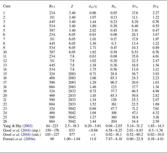
leads to similar values, as both quantities have the same order of magnitude in the present study. A total of 26 cases are investigated by varying the flow properties, and an overview of the main non-dimensional parameters is reported in table 3. For comparison, those parameters are listed also for relevant previous studies considering both air and water as working fluid, both experimental and computational. This underscores the vast range of
$W_0$
leads to similar values, as both quantities have the same order of magnitude in the present study. A total of 26 cases are investigated by varying the flow properties, and an overview of the main non-dimensional parameters is reported in table 3. For comparison, those parameters are listed also for relevant previous studies considering both air and water as working fluid, both experimental and computational. This underscores the vast range of $\tilde \rho$
and
$\tilde \rho$
and $ \textit{St}_\eta$
covered in this work.
$ \textit{St}_\eta$
covered in this work.
Size, density and dynamical properties of the investigated particles settling in air and water.
Main experimental parameters for all considered cases. Values are also reported for selected previous experimental and numerical studies.
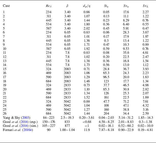
Table 3. Long description
The table presents a comparison of main non-dimensional parameters for 26 cases and selected previous experimental and numerical studies. It includes columns for case numbers, Reynolds number, dimensionless particle diameter, Stokes number in water, and Stokes number in air and liquid. Each row lists specific values for these parameters. The table also includes data from previous studies by Yang & Shy (2003), Good et al. (2014), and Fornari et al. (2016b), providing a comprehensive overview of the range of parameters investigated. The table is structured with 26 rows for the cases and additional rows for the previous studies, each row providing detailed numerical values for the parameters.
2.2. Measurement technique
In both air and water, the particles are located and tracked using a particle tracking velocimetry (PTV) algorithm based on a cross-correlation approach (Petersen et al. Reference Petersen, Baker and Coletti2019). A vertical plane at the centre of the chamber is illuminated using a double-pulsed Nd:YAG laser, synchronised with two 25-Megapixel CMOS cameras equipped with 100-mm focal length lenses. The cameras are placed side-by-side to capture a field of view extending 200 mm by 100 mm in the horizontal and vertical direction, respectively, around the geometric centre of the chambers. The inter-frame separation times are set to ensure a particle displacement of approximately 5 pixels. Image pairs are recorded at a sampling frequency of 2 Hz, providing approximately uncorrelated realisations. The PTV algorithm searches for a matching object within a specified radius around each particle centroid, maximising the correlation coefficient between image pairs. Depending on the cases, between 200 and 2000 realisations are acquired, resulting in $O(10^5)$
particle velocity vectors in each case. The large number of samples result in negligibly small statistical uncertainty. Possible sources of error might be the slight particle polydispersity and run-to-run variability of the turbulence properties. Repeatability tests and sensitivity analysis (incorporating the small polydispersity) indicate that such factors do not influence the quantitative conclusions.
$O(10^5)$
particle velocity vectors in each case. The large number of samples result in negligibly small statistical uncertainty. Possible sources of error might be the slight particle polydispersity and run-to-run variability of the turbulence properties. Repeatability tests and sensitivity analysis (incorporating the small polydispersity) indicate that such factors do not influence the quantitative conclusions.
In the water chamber, the fluid flow is measured simultaneously with the particle motion by particle image velocimetry (PIV) using tracers consisting of 30–55 ${\unicode{x03BC}} \text{m}$
hollow-glass spheres. Raw images are separated into particle-only and tracer-only images using an algorithm that identifies contiguous groups of pixels above a certain intensity threshold, classifying them based on size and intensity (Petersen et al. Reference Petersen, Baker and Coletti2019). The pixels attributed to an inertial particle are zeroed and filled with Gaussian noise and PIV is performed on the tracer-only images with an initial interrogation window of
${\unicode{x03BC}} \text{m}$
hollow-glass spheres. Raw images are separated into particle-only and tracer-only images using an algorithm that identifies contiguous groups of pixels above a certain intensity threshold, classifying them based on size and intensity (Petersen et al. Reference Petersen, Baker and Coletti2019). The pixels attributed to an inertial particle are zeroed and filled with Gaussian noise and PIV is performed on the tracer-only images with an initial interrogation window of $64\,\times \,64$
pixels, refined to
$64\,\times \,64$
pixels, refined to $32\,\times \,32$
pixels with 50 % overlap. Vector validation is carried out based on the signal-to-noise ratio and deviation from the median of neighbouring vectors (Adrian & Westerweel Reference Adrian and Westerweel2011), resulting in less than 5 % of rejected vectors in each set. The fluid velocity at particle locations are obtained through linear interpolation of the neighbouring velocity vectors (Berk & Coletti Reference Berk and Coletti2021).
$32\,\times \,32$
pixels with 50 % overlap. Vector validation is carried out based on the signal-to-noise ratio and deviation from the median of neighbouring vectors (Adrian & Westerweel Reference Adrian and Westerweel2011), resulting in less than 5 % of rejected vectors in each set. The fluid velocity at particle locations are obtained through linear interpolation of the neighbouring velocity vectors (Berk & Coletti Reference Berk and Coletti2021).
3. Results
3.1. Settling velocity
(a) Particles mean settling velocity normalised by the quiescent terminal velocity versus $Sv_L$
. (b) Particles turbulent settling speed difference versus
$Sv_L$
. (b) Particles turbulent settling speed difference versus $Sv_L$
.
$Sv_L$
.
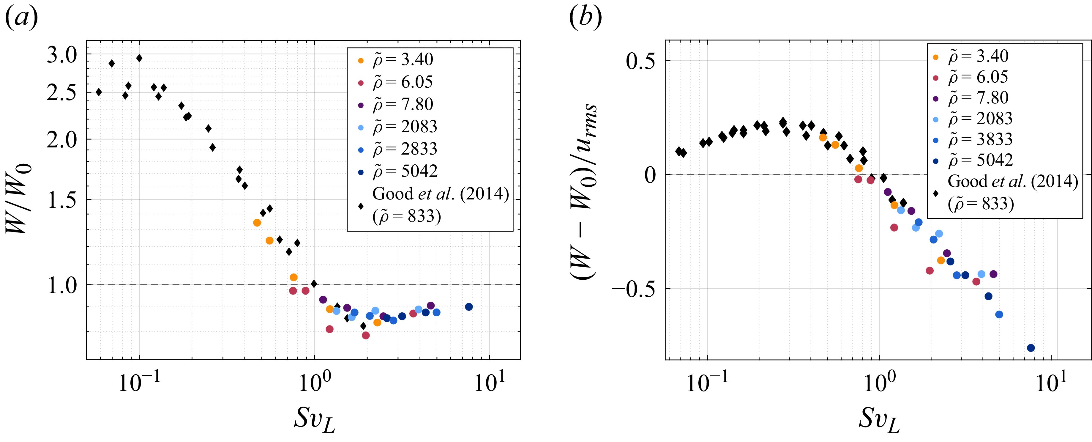
Figure 3(a) shows the normalised mean settling velocity, $W/W_0$
, as a function of
$W/W_0$
, as a function of $Sv_L$
. Both enhanced and hindered settling are observed, for small and large
$Sv_L$
. Both enhanced and hindered settling are observed, for small and large $Sv_L$
, respectively, with the transition occurring at
$Sv_L$
, respectively, with the transition occurring at $Sv_L \approx 1$
. Since such a parameter is the ratio of the turnover time of an integral-scale eddy
$Sv_L \approx 1$
. Since such a parameter is the ratio of the turnover time of an integral-scale eddy $(L/u_{\textit{rms}})$
and the time taken by a falling particle to cross such eddy
$(L/u_{\textit{rms}})$
and the time taken by a falling particle to cross such eddy $(L/W_0)$
, we interpret this result as follows: when
$(L/W_0)$
, we interpret this result as follows: when $Sv_L \lt 1$
, the particles have time to respond to the turbulence and experience preferential sweeping; while their trajectory is relatively unaffected for
$Sv_L \lt 1$
, the particles have time to respond to the turbulence and experience preferential sweeping; while their trajectory is relatively unaffected for $Sv_L \gt 1$
. In the latter case, loitering and nonlinear drag are expected to be prevalent due to the more rectilinear trajectories and relatively large slip velocities (Nielsen Reference Nielsen1993). The collapse of the present data across three decades of density ratio indicates that the latter does not play a significant role in the settling modification. As
$Sv_L \gt 1$
. In the latter case, loitering and nonlinear drag are expected to be prevalent due to the more rectilinear trajectories and relatively large slip velocities (Nielsen Reference Nielsen1993). The collapse of the present data across three decades of density ratio indicates that the latter does not play a significant role in the settling modification. As $Sv_L \to \infty$
, the settling velocity is expected return to
$Sv_L \to \infty$
, the settling velocity is expected return to $W_0$
, as the influence of the turbulence becomes negligible. Hints of this trend can be observed in figure 3(a), the settling being most hindered around
$W_0$
, as the influence of the turbulence becomes negligible. Hints of this trend can be observed in figure 3(a), the settling being most hindered around $Sv_L \approx 2$
for a fall speed reduction of approximately 20 %. Conversely, in the limit of
$Sv_L \approx 2$
for a fall speed reduction of approximately 20 %. Conversely, in the limit of $Sv_L \to 0$
, a return towards
$Sv_L \to 0$
, a return towards $W_0$
is expected, as particles with negligible inertia and settling velocity tend to follow the fluid. Therefore, the settling enhancement is expected to reach a maximum in the range
$W_0$
is expected, as particles with negligible inertia and settling velocity tend to follow the fluid. Therefore, the settling enhancement is expected to reach a maximum in the range $0 \lt Sv_L\lt 1$
, as clearly visible in figures 3(a) and 3(b). More data are needed to determine the position and value of such a maximum and its dependence with the governing parameters. The alternative normalisation of the settling velocity,
$0 \lt Sv_L\lt 1$
, as clearly visible in figures 3(a) and 3(b). More data are needed to determine the position and value of such a maximum and its dependence with the governing parameters. The alternative normalisation of the settling velocity, $(W-W_0)/u_{\textit{rms}}$
, is plotted as a function of
$(W-W_0)/u_{\textit{rms}}$
, is plotted as a function of $Sv_L$
in figure 3(b). The data collapse highlights again the dominant role of the large scales of the turbulence. Plotting the normalised settling rate as function of other non-dimensional parameters does not yield similar collapse of the data.
$Sv_L$
in figure 3(b). The data collapse highlights again the dominant role of the large scales of the turbulence. Plotting the normalised settling rate as function of other non-dimensional parameters does not yield similar collapse of the data.
Experimental results on water droplets in air from Good et al. (Reference Good, Ireland, Bewley, Bodenschatz, Collins and Warhaft2014) are also plotted, showing excellent agreement with our data. The results from Good et al. (Reference Good, Ireland, Bewley, Bodenschatz, Collins and Warhaft2014) are chosen as representative of laboratory investigations in which, similarly to the present study, great care was taken to minimise confounding factors discussed in the paper, such as flow recirculation and uncertainty on the particle size. Furthermore, Good et al. (Reference Good, Ireland, Bewley, Bodenschatz, Collins and Warhaft2014) covered a wide range of $Sv_L$
, partly overlapping with ours but reaching lower values. Their data are also consistent with other works in similar ranges of parameters, e.g. Ferran et al. (Reference Ferran, Machicoane, Aliseda and Obligado2023) who also investigated water droplets in air, and Petersen et al. (Reference Petersen, Baker and Coletti2019) and Berk & Coletti (Reference Berk and Coletti2021) who studied glass spheres in air. In those previous studies,
$Sv_L$
, partly overlapping with ours but reaching lower values. Their data are also consistent with other works in similar ranges of parameters, e.g. Ferran et al. (Reference Ferran, Machicoane, Aliseda and Obligado2023) who also investigated water droplets in air, and Petersen et al. (Reference Petersen, Baker and Coletti2019) and Berk & Coletti (Reference Berk and Coletti2021) who studied glass spheres in air. In those previous studies, $d_p \lt \eta$
and
$d_p \lt \eta$
and $ \textit{Re}_{p,0} = O(10^{-2}\,$
–
$ \textit{Re}_{p,0} = O(10^{-2}\,$
– $\,1)$
, while here
$\,1)$
, while here $d_p =O(\eta )$
and
$d_p =O(\eta )$
and $ \textit{Re}_{p,0} = O(10)$
. Therefore, the transition between enhanced and reduced settling around
$ \textit{Re}_{p,0} = O(10)$
. Therefore, the transition between enhanced and reduced settling around $Sv_L \approx 1$
appears widely applicable in homogeneous turbulence. Additionally, our results can be compared with the model recently proposed by Peng et al. (Reference Peng, Karzhaubayev, Wang, Chen and Niu2025), who proposed a general formulation for the settling modification by turbulence as a function of
$Sv_L \approx 1$
appears widely applicable in homogeneous turbulence. Additionally, our results can be compared with the model recently proposed by Peng et al. (Reference Peng, Karzhaubayev, Wang, Chen and Niu2025), who proposed a general formulation for the settling modification by turbulence as a function of $d_p/\eta$
,
$d_p/\eta$
, $ \textit{Re}_{p,0}$
and
$ \textit{Re}_{p,0}$
and $Sv_L$
. Their model captures the general trend of the settling velocity decreasing with
$Sv_L$
. Their model captures the general trend of the settling velocity decreasing with $Sv_L$
in the considered parameter range. Discrepancies grow larger for levels of
$Sv_L$
in the considered parameter range. Discrepancies grow larger for levels of $Sv_L$
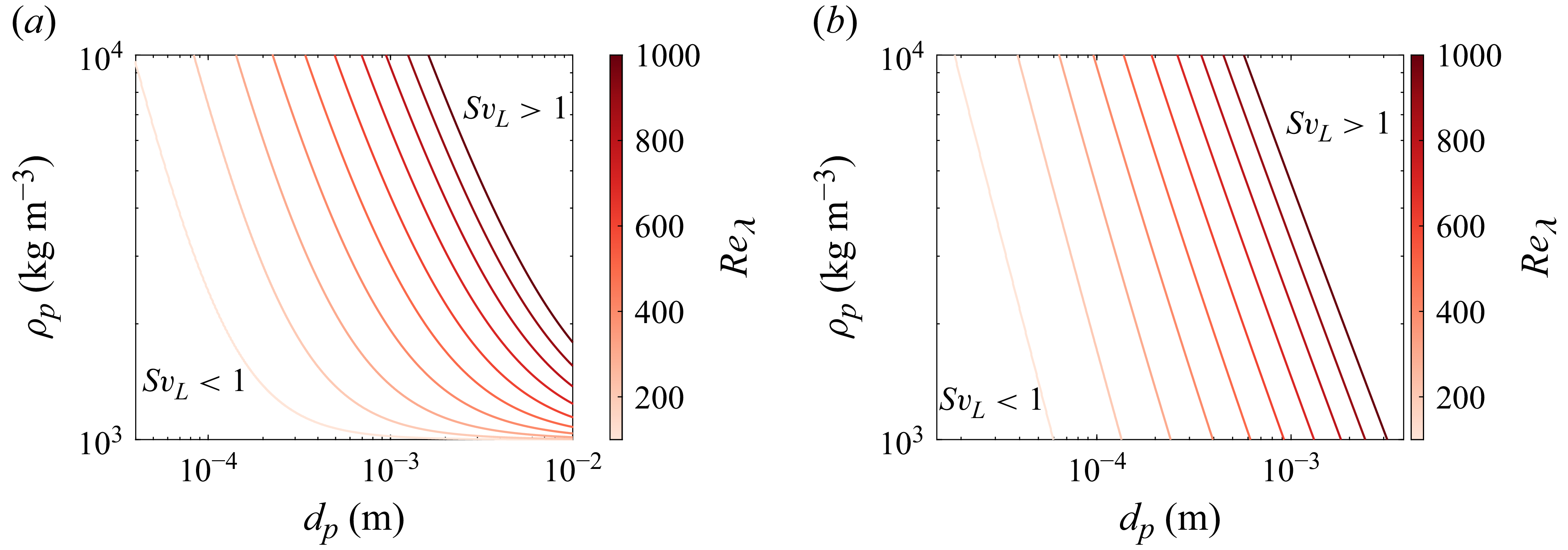
much smaller or larger than unity, suggesting that tuning of the model constants or additional physical considerations might be required to achieve a quantitative agreement across the parameter space. In figures 4(a) and 4(b), isolines at
$Sv_L$
much smaller or larger than unity, suggesting that tuning of the model constants or additional physical considerations might be required to achieve a quantitative agreement across the parameter space. In figures 4(a) and 4(b), isolines at $Sv_L = 1$
are plotted in the
$Sv_L = 1$
are plotted in the $d_p$
–
$d_p$
– $\rho _p$
plane, assuming water and air as working fluid, respectively, and for a range of
$\rho _p$
plane, assuming water and air as working fluid, respectively, and for a range of $ \textit{Re}_\lambda$
typical of laboratory installations. Common studies of sediment-type particles in water (plastic or sand with
$ \textit{Re}_\lambda$
typical of laboratory installations. Common studies of sediment-type particles in water (plastic or sand with $d_p \gt 1\, \text{mm}$
, e.g. Zhou & Cheng Reference Zhou and Cheng2009; Akutina et al. Reference Akutina, Revil-Baudard, Chauchat and Eiff2020) are usually in the region
$d_p \gt 1\, \text{mm}$
, e.g. Zhou & Cheng Reference Zhou and Cheng2009; Akutina et al. Reference Akutina, Revil-Baudard, Chauchat and Eiff2020) are usually in the region $Sv_L \gt 1$
, while water droplets and glass spheres with
$Sv_L \gt 1$
, while water droplets and glass spheres with $d_p \lt 50\,{\unicode{x03BC}} \text{m}$
in air (e.g. Aliseda et al. Reference Aliseda, Cartellier, Hainaux and Lasheras2002; Berk & Coletti Reference Berk and Coletti2021) tend to fall in the region
$d_p \lt 50\,{\unicode{x03BC}} \text{m}$
in air (e.g. Aliseda et al. Reference Aliseda, Cartellier, Hainaux and Lasheras2002; Berk & Coletti Reference Berk and Coletti2021) tend to fall in the region $Sv_L \lt 1$
. Those two classes of experiments form the bulk of the empirical evidence for reduced and enhanced settling by turbulence, respectively. Therefore, the opposite behaviour of settling enhancement/reduction often reported in turbulent air/water can be mapped to the transition happening around
$Sv_L \lt 1$
. Those two classes of experiments form the bulk of the empirical evidence for reduced and enhanced settling by turbulence, respectively. Therefore, the opposite behaviour of settling enhancement/reduction often reported in turbulent air/water can be mapped to the transition happening around $Sv_L =1$
.
$Sv_L =1$
.
Isolines at $Sv_L = 1$
in the
$Sv_L = 1$
in the $d_p$
–
$d_p$
– $\rho _p$
space, nominally separating the enhanced
$\rho _p$
space, nominally separating the enhanced $(Sv_L\lt 1)$
and hindered
$(Sv_L\lt 1)$
and hindered $(Sv_L\gt 1)$
regimes for different
$(Sv_L\gt 1)$
regimes for different $ \textit{Re}_\lambda$
, for both (a) water and (b) air.
$ \textit{Re}_\lambda$
, for both (a) water and (b) air.
3.2. Fluid velocity at the particle location
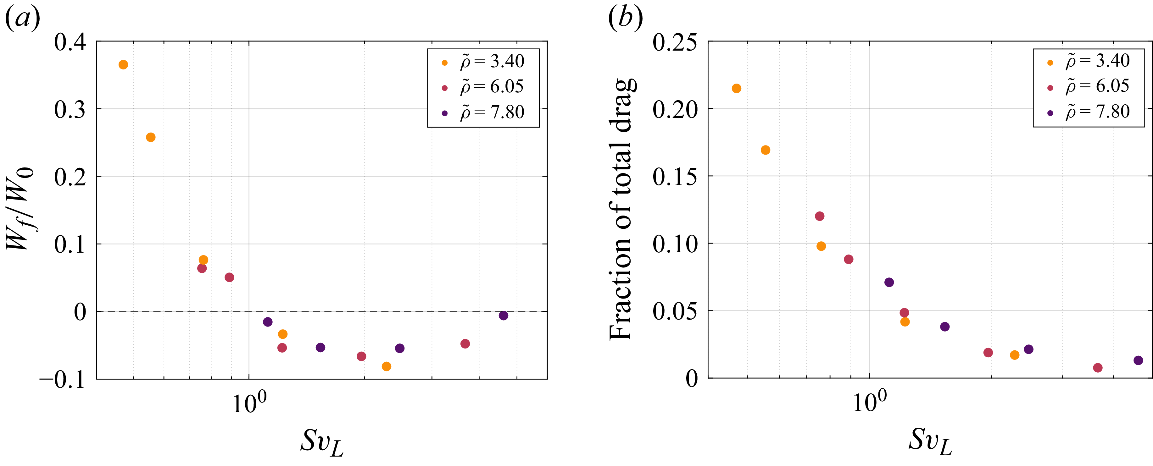
To better understand the mechanisms responsible for the modification of the particle settling rate, the fluid vertical velocity at the particle location is evaluated. This quantity is relevant to both preferential sweeping and loitering, the two being defined by the particles favouring downward and upward velocity fluctuations, respectively. Figure 5(a) shows the mean vertical fluid velocity at the particle location $W_{\kern-1pt f}$
, ensemble-averaged over all samples and normalised by
$W_{\kern-1pt f}$
, ensemble-averaged over all samples and normalised by $W_0$
, as a function of
$W_0$
, as a function of $Sv_L$
. The trend is consistent with our interpretation of the data in figure 3: for
$Sv_L$
. The trend is consistent with our interpretation of the data in figure 3: for $Sv_L\lt 1$
, the particles experience preferential sweeping, tending to oversample downward turbulent fluctuations; while for
$Sv_L\lt 1$
, the particles experience preferential sweeping, tending to oversample downward turbulent fluctuations; while for $Sv_L\gt 1$
, they experience loitering, spending more time descending against upward turbulent fluctuations. The most intense loitering is visible at
$Sv_L\gt 1$
, they experience loitering, spending more time descending against upward turbulent fluctuations. The most intense loitering is visible at $Sv_L \approx 2$
, corresponding to the strongest hindering of the settling rate. Even for this condition,
$Sv_L \approx 2$
, corresponding to the strongest hindering of the settling rate. Even for this condition, $W_{\kern-1pt f} = -0.07W_0$
; thus, the extent of the loitering is significantly smaller than the preferential sweeping, which reaches
$W_{\kern-1pt f} = -0.07W_0$
; thus, the extent of the loitering is significantly smaller than the preferential sweeping, which reaches $W_{\kern-1pt f} = 0.35W_0$
in the investigated range (and may be even larger for smaller
$W_{\kern-1pt f} = 0.35W_0$
in the investigated range (and may be even larger for smaller $Sv_L$
).
$Sv_L$
).
(a) Mean vertical fluid velocity at the particle location normalised by the quiescent terminal velocity versus $Sv_L$
. (b) Fractional contribution of nonlinear drag to the overall drag experienced by the settling particles, as a function of
$Sv_L$
. (b) Fractional contribution of nonlinear drag to the overall drag experienced by the settling particles, as a function of $Sv_L$
.
$Sv_L$
.
Knowledge of the fluid velocity at the particle location also allows us to evaluate the relative (slip) velocity between fluid and particle, which is essential to assess the effect of nonlinear drag. To quantify this effect, we follow Fornari et al. (Reference Fornari, Picano, Sardina and Brandt2016b ) and express the fractional contributions to the total drag as
 \begin{align} 1=\frac {W_{\textit{slip}}(1+\widehat {K})}{W_{0s}}+\frac {W_{\textit{slip}}K''}{W_{0s}}+\frac {\big\langle w_{\textit{slip}}'K' \big\rangle }{W_{0s}}+f_D^U ,\end{align}
where ${W_{0s}}=2(\rho _p - \rho _{\kern-1pt f})g(d_p/2)^2/(9\rho _{\kern-1pt f}\nu )$
is the Stokesian settling velocity and
${W_{0s}}=2(\rho _p - \rho _{\kern-1pt f})g(d_p/2)^2/(9\rho _{\kern-1pt f}\nu )$
is the Stokesian settling velocity and ${w}_{\textit{slip}}=W_{\textit{slip}}+w_{\textit{slip}}'$
is the vertical slip velocity, decomposed into its mean and fluctuation. The variable
${w}_{\textit{slip}}=W_{\textit{slip}}+w_{\textit{slip}}'$
is the vertical slip velocity, decomposed into its mean and fluctuation. The variable $K=\alpha Re_p^\beta$
is associated with the nonlinear drag correction due to the finite instantaneous Reynolds number
$K=\alpha Re_p^\beta$
is associated with the nonlinear drag correction due to the finite instantaneous Reynolds number $ \textit{Re}_p = d_pw_{\textit{slip}}/\nu$
; e.g.
$ \textit{Re}_p = d_pw_{\textit{slip}}/\nu$
; e.g. $\alpha =0.15$
and
$\alpha =0.15$
and $\beta = 0.687$
according to the Schiller–Neumann correlation. This quantity is in turn decomposed as
$\beta = 0.687$
according to the Schiller–Neumann correlation. This quantity is in turn decomposed as $K = \widehat {K} + K' + K''$
, with
$K = \widehat {K} + K' + K''$
, with $\widehat {K} = \alpha (d_pW_{\textit{slip}}/\nu )^\beta$
,
$\widehat {K} = \alpha (d_pW_{\textit{slip}}/\nu )^\beta$
, $K'=K-\langle \alpha Re_p^\beta \rangle$
and
$K'=K-\langle \alpha Re_p^\beta \rangle$
and $K''= \langle \alpha Re_p^\beta \rangle - \widehat {K}$
(angle brackets denoting ensemble-averaging). The first term on the right-hand side of (3.1) corresponds to the drag associated with the mean settling velocity; the second term accounts for the horizontal relative velocity between particle and fluid; the third term is associated with the effect of the fluctuating vertical relative velocity; and
$K''= \langle \alpha Re_p^\beta \rangle - \widehat {K}$
(angle brackets denoting ensemble-averaging). The first term on the right-hand side of (3.1) corresponds to the drag associated with the mean settling velocity; the second term accounts for the horizontal relative velocity between particle and fluid; the third term is associated with the effect of the fluctuating vertical relative velocity; and $f_D^U$
denotes unsteady effects such as particle–wake interactions; see Fornari et al. (Reference Fornari, Picano, Sardina and Brandt2016b
) for details. The second and third terms are associated with drag nonlinearity, as fluctuations of both the vertical slip velocity and the lateral cross-flow play no role in the linear drag regime (see Ruth et al. Reference Ruth, Vernet, Perrard and Deike2021; Tinklenberg, Guala & Coletti Reference Tinklenberg, Guala and Coletti2024).
$f_D^U$
denotes unsteady effects such as particle–wake interactions; see Fornari et al. (Reference Fornari, Picano, Sardina and Brandt2016b
) for details. The second and third terms are associated with drag nonlinearity, as fluctuations of both the vertical slip velocity and the lateral cross-flow play no role in the linear drag regime (see Ruth et al. Reference Ruth, Vernet, Perrard and Deike2021; Tinklenberg, Guala & Coletti Reference Tinklenberg, Guala and Coletti2024).
Figure 5(b) shows the fractional nonlinear contribution to the overall drag, i.e. the sum of the second and third terms on the left-hand side of (3.1). This exceeds 20 % at small $Sv_L$
, i.e. for relatively high turbulence intensity: the particles experience fluctuations of the slip velocity which are significant compared with their settling velocity. At large
$Sv_L$
, i.e. for relatively high turbulence intensity: the particles experience fluctuations of the slip velocity which are significant compared with their settling velocity. At large $Sv_L$
, however, those fluctuations are marginal compared with the fall speed and the nonlinear contribution amounts to less than 2 % of the total. Therefore, for the considered wide range of parameters, nonlinear drag effects are most prominent in the regime where the settling rate is overall enhanced. This is in contrast to the common view that nonlinear drag would be the cause of reduced settling velocity for small particles in turbulence. In the considered range of parameters, nonlinearity does act to decrease the settling velocity, but does so most significantly under conditions in which preferential sweeping is prominent and the overall fall speed is higher than in quiescent fluid.
$Sv_L$
, however, those fluctuations are marginal compared with the fall speed and the nonlinear contribution amounts to less than 2 % of the total. Therefore, for the considered wide range of parameters, nonlinear drag effects are most prominent in the regime where the settling rate is overall enhanced. This is in contrast to the common view that nonlinear drag would be the cause of reduced settling velocity for small particles in turbulence. In the considered range of parameters, nonlinearity does act to decrease the settling velocity, but does so most significantly under conditions in which preferential sweeping is prominent and the overall fall speed is higher than in quiescent fluid.
4. Discussion and conclusions
We have experimentally investigated the settling of heavy spherical particles in homogeneous turbulence, in both water and air. The ranges $ \textit{Re}_{p,0} = O(10)$
and
$ \textit{Re}_{p,0} = O(10)$
and $d_p/\eta = O(1)$
are typical of both sediment (Best Reference Best1988) and frozen precipitation (Guala & Hong Reference Guala and Hong2025), as well as many industrial processes (Zhou & Cheng Reference Zhou and Cheng2009). The use of large zero-mean-flow chambers stirred by randomised jet arrays reduces measurement biases and limits the influence of possibly confounding factors, such as secondary flow motions, mean shear/strain and flow inhomogeneities. The wide range of
$d_p/\eta = O(1)$
are typical of both sediment (Best Reference Best1988) and frozen precipitation (Guala & Hong Reference Guala and Hong2025), as well as many industrial processes (Zhou & Cheng Reference Zhou and Cheng2009). The use of large zero-mean-flow chambers stirred by randomised jet arrays reduces measurement biases and limits the influence of possibly confounding factors, such as secondary flow motions, mean shear/strain and flow inhomogeneities. The wide range of $\tilde \rho$
and
$\tilde \rho$
and $ \textit{St}_\eta$
and the simultaneous measurement of both particles and fluid motion provide novel quantitative insight on the effect of background turbulence on the settling rate.
$ \textit{St}_\eta$
and the simultaneous measurement of both particles and fluid motion provide novel quantitative insight on the effect of background turbulence on the settling rate.
We find that $Sv_L$
dictates settling enhancement and reduction, which occur for
$Sv_L$
dictates settling enhancement and reduction, which occur for $Sv_L$
smaller and larger than unity, respectively. This reflects the particles’ (in)ability to respond to the eddies they cross in their descent, resulting in biased sampling of the flow field:
$Sv_L$
smaller and larger than unity, respectively. This reflects the particles’ (in)ability to respond to the eddies they cross in their descent, resulting in biased sampling of the flow field: $Sv_L \lt 1$
allows for preferential sweeping, while
$Sv_L \lt 1$
allows for preferential sweeping, while $Sv_L \gt 1$
leads to loitering. The general picture was discussed in previous studies (e.g. Nielsen Reference Nielsen1993; Good et al. Reference Good, Ireland, Bewley, Bodenschatz, Collins and Warhaft2014; Rosa et al. Reference Rosa, Parishani, Ayala and Wang2016; Baker et al. Reference Baker, Frankel, Mani and Coletti2017; Tom & Bragg Reference Tom and Bragg2019) and other parameters were proposed to characterise the transition from enhanced to reduced settling, e.g.
$Sv_L \gt 1$
leads to loitering. The general picture was discussed in previous studies (e.g. Nielsen Reference Nielsen1993; Good et al. Reference Good, Ireland, Bewley, Bodenschatz, Collins and Warhaft2014; Rosa et al. Reference Rosa, Parishani, Ayala and Wang2016; Baker et al. Reference Baker, Frankel, Mani and Coletti2017; Tom & Bragg Reference Tom and Bragg2019) and other parameters were proposed to characterise the transition from enhanced to reduced settling, e.g. $ \textit{St}_\eta Sv_L$
(Nemes et al. Reference Nemes, Dasari, Hong, Guala and Coletti2017; Petersen et al. Reference Petersen, Baker and Coletti2019; Ferran et al. Reference Ferran, Machicoane, Aliseda and Obligado2023). This study presents clear evidence that
$ \textit{St}_\eta Sv_L$
(Nemes et al. Reference Nemes, Dasari, Hong, Guala and Coletti2017; Petersen et al. Reference Petersen, Baker and Coletti2019; Ferran et al. Reference Ferran, Machicoane, Aliseda and Obligado2023). This study presents clear evidence that $Sv_L$
is the decisive parameter, showing its key role in the switch between preferential sweeping and loitering at
$Sv_L$
is the decisive parameter, showing its key role in the switch between preferential sweeping and loitering at $Sv_L\approx 1$
, as demonstrated by measurements of the fluid velocity at the particle location. This result, along with typical ranges of parameters in laboratory experiments, explains the observation that particles in water and air tend to experience settling reduction and enhancement, respectively.
$Sv_L\approx 1$
, as demonstrated by measurements of the fluid velocity at the particle location. This result, along with typical ranges of parameters in laboratory experiments, explains the observation that particles in water and air tend to experience settling reduction and enhancement, respectively.
The role of $Sv_L$
also signals the crucial importance of the energetic scales of the turbulence in affecting the particle fall speed, as opposed to the Kolmogorov scales that have long been recognised to drive the highest level of clustering (Wang & Maxey Reference Wang and Maxey1993; Eaton & Fessler Reference Eaton and Fessler1994). This view is consistent with the theoretical analysis of Tom & Bragg (Reference Tom and Bragg2019): they argued that the flow scales responsible for preferential sweeping increase with particle inertia and, even for relatively small
$Sv_L$
also signals the crucial importance of the energetic scales of the turbulence in affecting the particle fall speed, as opposed to the Kolmogorov scales that have long been recognised to drive the highest level of clustering (Wang & Maxey Reference Wang and Maxey1993; Eaton & Fessler Reference Eaton and Fessler1994). This view is consistent with the theoretical analysis of Tom & Bragg (Reference Tom and Bragg2019): they argued that the flow scales responsible for preferential sweeping increase with particle inertia and, even for relatively small $ \textit{St}_\eta$
, such scales would be orders of magnitude larger than
$ \textit{St}_\eta$
, such scales would be orders of magnitude larger than $\eta$
, thus comparable to
$\eta$
, thus comparable to $L$
for the range of
$L$
for the range of $ \textit{Re}_\lambda$
considered here.
$ \textit{Re}_\lambda$
considered here.
The present and previous data (e.g. Aliseda et al. Reference Aliseda, Cartellier, Hainaux and Lasheras2002; Good et al. Reference Good, Ireland, Bewley, Bodenschatz, Collins and Warhaft2014; Petersen et al. Reference Petersen, Baker and Coletti2019) indicate that, compared with still-fluid conditions, settling velocities are more than doubled by turbulence when $Sv_L = O(10^{-1})$
, while they are reduced by approximately 20 % when
$Sv_L = O(10^{-1})$
, while they are reduced by approximately 20 % when $Sv_L \approx 2$
. These levels are quantitatively influenced by nonlinear drag effects, which are investigated here using the instantaneously measured particle–fluid relative velocity. At odds with the prevalent view, it is found that drag nonlinearity is mostly influential for relatively small
$Sv_L \approx 2$
. These levels are quantitatively influenced by nonlinear drag effects, which are investigated here using the instantaneously measured particle–fluid relative velocity. At odds with the prevalent view, it is found that drag nonlinearity is mostly influential for relatively small $Sv_L$
, i.e. in the regime of settling enhancement, while its contribution to settling reduction at large
$Sv_L$
, i.e. in the regime of settling enhancement, while its contribution to settling reduction at large $Sv_L$
is modest. The hindering of settling in homogeneous turbulence is largely due to loitering.
$Sv_L$
is modest. The hindering of settling in homogeneous turbulence is largely due to loitering.
A quantitative comparison of the preferential sampling and the change in settling velocity highlights the limitations of the standard point-particle approximation. According to the latter, one expects the settling enhancement/reduction to correspond to the average downward/upward fluid velocity sampled by the particles (Wang & Maxey Reference Wang and Maxey1993). Our measurements indicate that this can greatly underestimate both the enhancement of the settling rate (as already found by Petersen et al. Reference Petersen, Baker and Coletti2019) and its reduction. This is likely due to multiple factors. One is certainly the drag nonlinearity, which results in an effective drag coefficient smaller than the nominal one based on the average slip velocity (as discussed by Balachandar & Eaton (Reference Balachandar and Eaton2010) and Petersen et al. (Reference Petersen, Baker and Coletti2019)). Moreover, the empirical correlations used to correct for such nonlinearity are based on simplistic assumptions of uniform and steady flow. While the Schiller–Neumann correlation fared well against the experiments of Bergougnoux et al. (Reference Bergougnoux, Bouchet, Lopez and Guazzelli2014), those were conducted at relatively small Stokes and Reynolds numbers. Our results, however, indicate that nonlinear drag effects are not sufficient to explain the large mismatch between experiments and simulations. An additional factor may be the one-way coupling assumption that the particles would not locally affect the flow. This is likely to break down even at the moderate values of $d_p/\eta$
and
$d_p/\eta$
and $ \textit{Re}_{p,0}$
considered here, as recently shown by the particle-resolved simulations of Chiarini et al. (Reference Chiarini, Tandurella and Rosti2025). Both analytical (e.g. Horowitz & Mani Reference Horowitz and Mani2016) and data-driven strategies (e.g. Siddani & Balachandar Reference Siddani and Balachandar2023) have been proposed to incorporate effective corrections to the point-particle approach, and the present results may inform such modelling efforts.
$ \textit{Re}_{p,0}$
considered here, as recently shown by the particle-resolved simulations of Chiarini et al. (Reference Chiarini, Tandurella and Rosti2025). Both analytical (e.g. Horowitz & Mani Reference Horowitz and Mani2016) and data-driven strategies (e.g. Siddani & Balachandar Reference Siddani and Balachandar2023) have been proposed to incorporate effective corrections to the point-particle approach, and the present results may inform such modelling efforts.
While we have covered a wide range of particle and fluid flow properties, the problem of settling modification by turbulence lives in a much broader parameter space. The present considerations apply in the considered range of particle Reynolds number; nonlinear drag, for example, may play a more important role in the settling reduction of larger/heavier particles with $ \textit{Re}_{p,0} = O(10^2{-}10^3)$
(Zhou & Cheng Reference Zhou and Cheng2009; Akutina et al. Reference Akutina, Revil-Baudard, Chauchat and Eiff2020). Furthermore, particles much larger than the Kolmogorov scales are known to exhibit different behaviours: partly because they act as spatial filters, interacting primarily with turbulent scales comparable to or larger than their diameter, and partly because they induce significant local flow modifications (Brandt & Coletti Reference Brandt and Coletti2022; Peng et al. Reference Peng, Karzhaubayev, Wang, Chen and Niu2025). Moreover, further analyses are needed to discern the quantitative influence on the settling rate of unsteady forces such as added mass and Basset-history force (Ling et al. Reference Ling, Parmar and Balachandar2013; Olivieri et al. Reference Olivieri, Picano, Sardina, Iudicone and Brandt2014), which have recently been shown to influence settling particularly in wall-bounded flows (Li, Bragg & Katul Reference Li, Bragg and Katul2023) along with other mechanisms specific to non-homogeneous turbulence (Bragg, Richter & Wang Reference Bragg, Richter and Wang2021). Finally, while non-spherical particles have attracted much interest in recent years (Voth & Soldati Reference Voth and Soldati2017; Marchioli et al. Reference Marchioli2025), the investigation of how turbulence modifies their gravitational settling is still in its infancy. Valuable insight has come from recent experiments (Kuperman, Sabban & Van Hout Reference Kuperman, Sabban and Van Hout2019; Esteban, Shrimpton & Ganapathisubramani Reference Esteban, Shrimpton and Ganapathisubramani2020; Tinklenberg et al. Reference Tinklenberg, Guala and Coletti2024; Tinklenberg, Guala & Coletti Reference Tinklenberg, Guala and Coletti2025; Bhowmick et al. Reference Bhowmick, Wang, Latt and Bagheri2025) and simulations (Ardekani et al. Reference Ardekani, Sardina, Brandt, Karp-Boss, Bearon and Variano2017; Sheikh et al. Reference Sheikh, Gustavsson, Lopez, Lévêque, Mehlig, Pumir and Naso2020; Moriche et al. Reference Moriche, Hettmann, García-Villalba and Uhlmann2023; Piumini et al. Reference Piumini, Assen, Lohse and Verzicco2024). More systematic efforts, however, are needed to reach a comprehensive picture.
$ \textit{Re}_{p,0} = O(10^2{-}10^3)$
(Zhou & Cheng Reference Zhou and Cheng2009; Akutina et al. Reference Akutina, Revil-Baudard, Chauchat and Eiff2020). Furthermore, particles much larger than the Kolmogorov scales are known to exhibit different behaviours: partly because they act as spatial filters, interacting primarily with turbulent scales comparable to or larger than their diameter, and partly because they induce significant local flow modifications (Brandt & Coletti Reference Brandt and Coletti2022; Peng et al. Reference Peng, Karzhaubayev, Wang, Chen and Niu2025). Moreover, further analyses are needed to discern the quantitative influence on the settling rate of unsteady forces such as added mass and Basset-history force (Ling et al. Reference Ling, Parmar and Balachandar2013; Olivieri et al. Reference Olivieri, Picano, Sardina, Iudicone and Brandt2014), which have recently been shown to influence settling particularly in wall-bounded flows (Li, Bragg & Katul Reference Li, Bragg and Katul2023) along with other mechanisms specific to non-homogeneous turbulence (Bragg, Richter & Wang Reference Bragg, Richter and Wang2021). Finally, while non-spherical particles have attracted much interest in recent years (Voth & Soldati Reference Voth and Soldati2017; Marchioli et al. Reference Marchioli2025), the investigation of how turbulence modifies their gravitational settling is still in its infancy. Valuable insight has come from recent experiments (Kuperman, Sabban & Van Hout Reference Kuperman, Sabban and Van Hout2019; Esteban, Shrimpton & Ganapathisubramani Reference Esteban, Shrimpton and Ganapathisubramani2020; Tinklenberg et al. Reference Tinklenberg, Guala and Coletti2024; Tinklenberg, Guala & Coletti Reference Tinklenberg, Guala and Coletti2025; Bhowmick et al. Reference Bhowmick, Wang, Latt and Bagheri2025) and simulations (Ardekani et al. Reference Ardekani, Sardina, Brandt, Karp-Boss, Bearon and Variano2017; Sheikh et al. Reference Sheikh, Gustavsson, Lopez, Lévêque, Mehlig, Pumir and Naso2020; Moriche et al. Reference Moriche, Hettmann, García-Villalba and Uhlmann2023; Piumini et al. Reference Piumini, Assen, Lohse and Verzicco2024). More systematic efforts, however, are needed to reach a comprehensive picture.
Funding
We gratefully acknowledge funding from the ERC consolidator grant EXPAT (REF-1131-52105) funded by the Swiss State Secretariat for Education, Research and Innovation, as well as from the Swiss National Science Foundation (Project No. 212065).
Declaration of interests
The authors report no conflict of interest.

 SvL
SvL ρ~
ρ~ Stη−Svη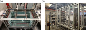

 SvL
SvL SvL
SvL
 SvL=1
SvL=1 dp
dp ρp
ρp (SvL<1)
 (SvL>1)
 Reλ
Reλ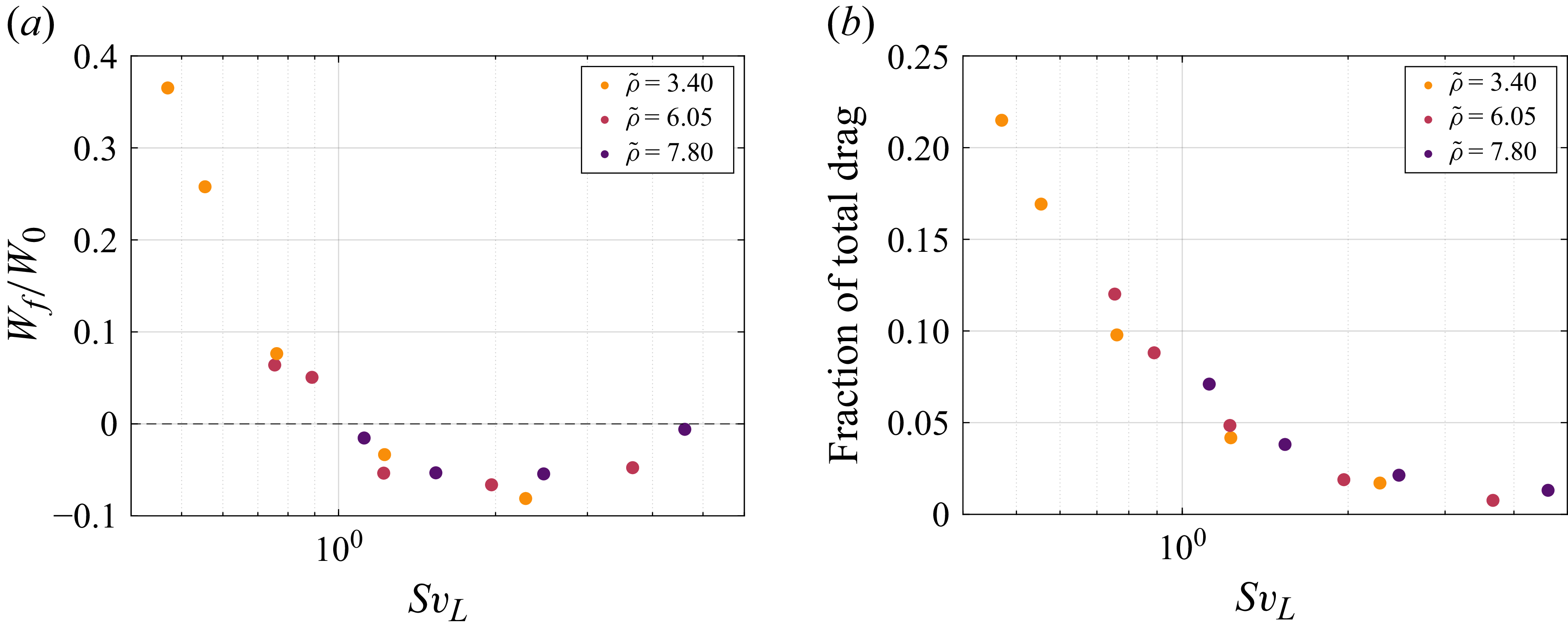
 SvL
SvL SvL
SvL
 Open access

