





Introduction
Paleoecological, sedimentological, and oxygen isotopic records of post-glacial environmental change show broad similarities across the northeastern United States during the Late Pleistocene. After the Laurentide ice sheet’s influence on regional climate waned, however, finer-scale spatial and temporal variability in climate, geography, and soils led to different watershed and ecosystem histories during the Holocene (Mandl et al., Reference Mandl, Shuman, Marsicek and Grigg2016; Shuman and Marsicek, Reference Shuman and Marsicek2016; Oswald et al., Reference Oswald, Foster, Shuman, Doughty, Faison, Hall, Hansen, Lindbladh, Marroquin and Truebe2018). Southern New England (Connecticut, Massachusetts, and Rhode Island) has been particularly well studied, with lake sediment cores taken from sites extending from the coast to interior uplands (Oswald et al., Reference Oswald, Foster, Shuman, Doughty, Faison, Hall, Hansen, Lindbladh, Marroquin and Truebe2018). In general, these sites show increasing moisture throughout the Holocene, a trend interrupted by multi-century periods of drought that have been tied to colder air temperatures over Greenland (Shuman et al., Reference Shuman, Newby and Donnelly2009; Newby et al., Reference Newby, Shuman, Donnelly, Karnauskas and Marsicek2014) or to cooler sea surface temperatures (SSTs) in the North Atlantic brought about by meltwater releases from the retreating Laurentide ice sheet and their effects on the Atlantic Meridional Overturning Circulation (Newby et al., Reference Newby, Donnelly, Shuman and MacDonald2009, Reference Newby, Shuman, Donnelly and MacDonald2011; Marsicek et al., Reference Marsicek, Shuman, Brewer, Foster and Oswald2013). Across sites, timing of droughts was commonly synchronous, although in the time interval 5600–4900 cal yr BP, drying in the western part of New England occurred earlier than in the east (Newby et al., Reference Newby, Shuman, Donnelly, Karnauskas and Marsicek2014).
While southern New England saw a general trend toward increasing moisture throughout the Holocene, the same is not true for the Northeast as a whole (Shuman et al., Reference Shuman, Newby, Huang and Webb2004; Munroe, Reference Munroe2012; Grigg et al., Reference Grigg, Stefanescu, Shuman and Oswald2023). Webb et al. (Reference Webb, Anderson and Webb1993) showed that spatial gradients in precipitation and soil moisture, reconstructed from fossil pollen records, were quite variable across the region and actually reversed orientation over time. Similarly, at the same time that conditions were getting wetter in Connecticut and Massachusetts, central New York appears to have become gradually drier. Lakes Cayuga and Owasco (Fig. 1) reached high stands around 12,400 cal yr BP (reported as ca. 10,500 14C yr BP), followed by oscillations toward lower lake levels at present (Dwyer et al., Reference Dwyer, Mullins and Good1996; Mullins, Reference Mullins1998). At Lake Cayuga, periods of wetter climate, approximately 1500 years apart, were superimposed on the general drying trend, and Lake Owasco saw a second small highstand at ca. 7800 cal yr BP (reported as 6900 14C yr BP) before declining.
Study area. (a) Global and regional setting. State labels are as follows: NY = New York; PA = Pennsylvania; NJ = New Jersey; CT = Connecticut; RI = Rhode Island; MA = Massachusetts; VT = Vermont; NH = New Hampshire; and ME = Maine. Black dots show the locations of comparison sites referenced in the text: AHP = Adirondack High Peaks lakes (Upper Wallface Pond and Heart Lake); BaL = Balsam Lake; BB = Brandreth Bog; BD = Blanding Lake; BL = Ballston Lake; BP = Blood Pond; CL = Cayuga Lake; CR = Crooked Pond; DP = Davis Pond; EL = Echo Lake; GL = Grinnell Lake; KH = Knob Hill Pond; LP = Little Pond; MC = Makepeace Cedar Swamp; MF = Maplecrest Fen; NH = Niles Huyck Bog; NL = New Long Pond; NP = North Pond; OL = Owasco Lake; RP = Rocky Pond; SF = Sunfish Pond; SL = Sluice Pond; SuP = Sutherland Pond; SpP = Spruce Pond; SR = lakes Minnewaska and Mohonk on the Shawangunk Ridge; TP = Twin Ponds; and WL = White Lake. Location of (b) is shown by the dark gray dashed-line box. (b) Location of Dyken and Shaver ponds on the Rensselaer Plateau. (c, d) Bathymetric maps of Shaver and Dyken ponds. Stars mark the locations where Livingstone cores were taken. Bathymetry data from https://www.dec.ny.gov/outdoor/84682.html (accessed February 27, 2025) and https://www.dec.ny.gov/outdoor/67414.html (accessed February 27, 2025).

Figure 1 Long description
A) A regional map of the northeastern USA, highlighting states such as New York (NY), Pennsylvania (PA), New Jersey (NJ), Connecticut (CT), Rhode Island (RI), Massachusetts (MA), Vermont (VT), New Hampshire (NH) and Maine (ME). Black dots indicate locations of various comparison sites like Adirondack High Peaks lakes, Balsam Lake and others. B) A detailed map of the Rensselaer Plateau, showing the locations of Shaver Pond and Dyken Pond, with nearby cities like Albany and Bennington marked. C) A bathymetric map of Shaver Pond with contour intervals of 10 feet, showing depth variations. D) A bathymetric map of Dyken Pond with contour intervals of 5 feet, illustrating depth changes. Both bathymetric maps include stars marking locations where Livingstone cores were taken.
Noting the discrepancy in conditions between New England and central New York, Menking et al. (Reference Menking, Peteet and Anderson2012) reconstructed the climate history of the Shawangunk Ridge in southeastern New York (Fig. 1) and found evidence that this area of elevated topography lies at or near a climatic divide separating the two regions. Like New England, the Ridge experienced dry conditions at the start of the Holocene that gave way to wetter conditions after 8700 cal yr BP. However, a ca. 1600-year-long dry interval in the Middle Holocene (5700–4100 cal yr BP) that coincided with falling Cayuga and Owasco Lake levels started at a time when some parts of New England were relatively wet (Shuman et al., Reference Shuman, Newby, Huang and Webb2004), and although New England also experienced drought from 5400 to 3000 cal yr BP, those conditions lasted nearly a millennium longer than on the Ridge (Newby et al., Reference Newby, Killoran, Waldorf, Shuman, Webb and Webb2000; Shuman et al., Reference Shuman, Newby, Huang and Webb2004).
The variable histories throughout the Northeast render challenging the interpretation of ecological shifts such as the well-known Mid-Holocene decline in Tsuga canadensis (eastern hemlock, henceforth Tsuga) (Marsicek et al., Reference Marsicek, Shuman, Brewer, Foster and Oswald2013). While this taxon appears to have dropped in abundance rather suddenly beginning around ca. 5500 cal yr BP in most locations (Bennett and Fuller, Reference Bennett and Fuller2002; Oswald et al., Reference Oswald, Foster, Shuman, Doughty, Faison, Hall, Hansen, Lindbladh, Marroquin and Truebe2018), the die-off in some areas appears to have coincided with warm conditions, whereas in others, cooling has been implicated (Foster et al., Reference Foster, Oswald, Faison, Doughty and Hansen2006; Marsicek et al., Reference Marsicek, Shuman, Brewer, Foster and Oswald2013; Oswald et al., Reference Oswald, Foster, Shuman, Doughty, Faison, Hall, Hansen, Lindbladh, Marroquin and Truebe2018; Grigg et al., Reference Grigg, Stefanescu, Shuman and Oswald2023). Whether conditions were wetter or drier than the preceding interval of Tsuga abundance varied among sites, with differing responses of coastal (moist) versus inland (dry, except in Vermont; Grigg et al., Reference Grigg, Stefanescu, Shuman and Oswald2023) locations (Newby et al., Reference Newby, Shuman, Donnelly, Karnauskas and Marsicek2014; Shuman and Burrell, Reference Shuman and Burrell2017; Oswald et al., Reference Oswald, Foster, Shuman, Doughty, Faison, Hall, Hansen, Lindbladh, Marroquin and Truebe2018).
On the Shawangunk Ridge, the collapse of Tsuga appears to have occurred in conjunction with warm and dry conditions, which caused frequent forest fires that favored Pinus rigida (pitch pine) and led to greater erosion, increasing clastic sedimentation, and charcoal deposition in ridge-top lakes Mohonk and Minnewaska (Menking et al., Reference Menking, Peteet and Anderson2012). In contrast, while drought was clearly implicated in a transient Tsuga decline at 8200 cal yr BP (reported as 7500 14C yr BP) at North Pond in western Massachusetts (Fig. 1), the classical Tsuga decline at 5500 cal yr BP coincided with no obvious signs of drying at that site (Huvane and Whitehead, Reference Huvane and Whitehead1996).
To add further confusion, a handful of records show younger timing of the Tsuga decline than the generally accepted period of ca. 5500–5000 cal yr BP. Records from southeastern New York’s Hudson Highlands, for example, show that the taxon collapsed at 4700 cal yr BP (reported as 4180 14C yr BP) at Sutherland Pond and near 3800 cal yr BP (reported as 3540 14C yr BP) at Spruce Pond (Fig. 1; Maenza-Gmelch, Reference Maenza-Gmelch1997), with no clear relationship to climate at either site. Indeed, some studies have questioned whether the Tsuga decline may have been driven by an insect pest or pathogen rather than by or in addition to climate change (Davis, Reference Davis, Bharadwaj, Vishnu-Mittre and Maheshwari1981; Bhiry and Filion, Reference Bhiry and Filion1996; Oswald et al., Reference Oswald, Doughty, Foster, Shuman and Wagner2017), although recent work by Shuman et al. (Reference Shuman, Stefanescu, Grigg, Foster and Oswald2023) suggests that variations in the latitudinal temperature gradient in New England, brought about primarily by changes in insolation, may have reduced the temperature conditions favorable to the taxon at the time of its collapse.
The complexity of climatic drivers and vegetational responses across the Northeast argues for the collection of additional records of late-glacial and Holocene ecological change (Menking et al., Reference Menking, Peteet and Anderson2012; Shuman and Marsicek, Reference Shuman and Marsicek2016; Oswald et al., Reference Oswald, Foster, Shuman, Doughty, Faison, Hall, Hansen, Lindbladh, Marroquin and Truebe2018). Here, we use pollen, plant macrofossils, sediment chemistry, and selected diatom time series to construct two new records from the previously unstudied Rensselaer Plateau, an area of elevated topography in eastern New York near the New York/Vermont/Massachusetts borders (Fig. 1). Sediment cores from Dyken and Shaver ponds allow us to address four questions. (1) When did forest first arrive on the Rensselaer Plateau and how did different taxa change over time? (2) What does the record of ecological variability tell us about climate change throughout the Holocene? (3) What does the record of aquatic ecosystem change add to interpretations of climate changes garnered from pollen and macrofossil studies? (4) What climatic conditions were associated with the Mid-Holocene Tsuga decline and when did the decline occur?
Like the Shawangunk Ridge, the Rensselaer Plateau’s location lies intermediate between New England and central New York, suggesting a potentially complex climate change history and associated ecological responses that may help shed additional light on regional drivers of climatic variability.
Study setting
The Rensselaer Plateau (Fig. 1) consists of 47,750 hectares of Silurian-age carbonate-cemented graywacke uplifted during the Taconic Orogeny and later overlain by glacial till associated with the Laurentide ice sheet (Ondrick, Reference Ondrick1968; https://www.rensselaerplateau.com/about-the-plateau-c1ulz, accessed May 23, 2025). Elevations range from 305 to ca. 550 m, yielding a climate more similar to the southern Adirondack Mountains to the northwest than to the Hudson Valley region immediately adjacent to the Plateau. Average January and July temperatures in the town of Grafton, located between the two lakes, measured −6 and 20°C, respectively, over a 30-year period from 1981 to 2010 (Arguez et al., Reference Arguez, Durre, Applequist, Squires, Vose, Yin and Bilotta2010), and average annual precipitation measured 121 cm. Rain and snow were distributed fairly evenly throughout the year, with summer months slightly wetter than the rest of the year.
Primary soil types on the Plateau consist of moderately to poorly drained, acidic, very stony loams and silt loams developed on glacial till (Work et al., Reference Work, Broad, Carlisle, Cassidy, Goodman, Landry and Mangum1988). These soils host a diverse assemblage of ecological communities, including hemlock–northern hardwood forest, beech–maple mesic forest, Appalachian oak–pine forest, maple–basswood-rich mesic forest, Appalachian oak–hickory forest, spruce–northern hardwood forest, and balsam flats and swamps, among others (https://www.rensselaerplateau.com/_files/ugd/394ce1_5f577a24ce954e8faa374b7dd246c62e.pdf; accessed January 17, 2026); and the Plateau is home to the fifth largest continuously forested area in New York state due to minimal human development (https://www.rensselaerplateau.com/about-the-plateau-c1ulz; accessed May 23, 2025).
Dyken Pond (42°43.33′N, 73°25.70′W) lies near the center of the Plateau at an elevation of 495 m and consists of two glacial kettles that merged after damming of the outlet of the southern pond in the 1800s to provide hydropower to textile, paper, and saw mills downstream. The dam is thought to have raised the lake level by around 4.6 m (Kane, Reference Kane2008), meaning that the 15-foot contour line (Fig. 1d) may represent the original outlet level, but evidence is scant. The lake presently measures 54 hectares in area and has maximum depths of 10.7 m in the northern basin and 6.1 m in the southern basin (Dyken, Reference Dyken Pondn.d.). The lake margin is forested with the exception of a few locations where lawns associated with single-family homes abut the shore (<5% of the shoreline).
Shaver Pond (42°46.83′N, 73°27.42′W) is located in the northwestern part of the Plateau and is one of six water bodies that collectively constitute the Grafton Lakes. It lies at 448 m elevation, measures 17.8 hectares in area, and has a maximum depth of 17 m (Shaver, Reference Shaver Pondn.d.). With the exception of a small wetland at the lake’s northern boundary, the entire shoreline is forested up to the lake edge (∼95% of the shoreline). Like Dyken Pond, Shaver Pond lacks any inflow streams of significant size but has an outlet, and both streams are part of the larger Hudson River watershed. Dyken Pond is a mesotrophic, softwater lake (Scavia, Reference Scavia1972) whereas Shaver Pond is meso-oligotrophic (New York State Office of Parks, Recreation, and Historic Preservation, 2012) and has a circum-neutral pH.
Methods
Core extraction
Sediment cores were extracted from Dyken and Shaver ponds (Fig. 1) in winter using Livingstone piston corers (Wright et al., Reference Wright, Mann and Glaser1984) lowered through holes in the frozen lake surface. Extruded cores were wrapped in plastic wrap, placed in capped, thick-walled PVC pipe (Dyken) or capped PVC D-tubes (Shaver), and refrigerated in cold rooms kept at 4°C at Vassar and Union colleges prior to sampling. The Dyken Pond core was taken in 2018 by students from Vassar College. It consists of five 1-m-long drives extracted from the same hole, with a PVC pipe column extending the entire length of the water column (5.9 m) used to guide the corer. Shaver Pond was cored in 1997 by students from Union College. Two adjacent and stratigraphically overlapping cores (A and C) were retrieved in 1-m drives through 17 m of water. Magnetic susceptibility measurements were used to correlate the two cores, allowing the record of the first core to be extended backward in time. The Shaver Pond cores were transferred to Vassar in 2020 for paleoecological analysis. All cores were split and described prior to sampling.
Laboratory analyses
Dating
Plant macrofossils and pieces of charcoal were extracted from each core for the purpose of accelerator mass spectrometer (AMS) radiocarbon dating. Bulk samples of gyttja from selected intervals were gently washed through 125-μm sieves to separate datable materials such as seeds, wood, charcoal, and leaf fragments. Macrofossils were then analyzed for dating by Beta Analytic Laboratory in Miami, Florida, and the Center for Accelerator Mass Spectrometry at Lawrence Livermore National Laboratory in Livermore, California. Radiocarbon dates were converted to calendar ages using the Bacon package in the R statistical software with the IntCal20 calibration (Blaauw and Christen, Reference Blaauw and Christen2011; Reimer et al., Reference Reimer, Austin, Bard, Bayliss, Blackwell, Bronk Ramsey and Butzin2020). Bacon was also used to construct the age model for each core.
Sediment chemistry and loss on ignition (LOI)
For Dyken Pond, 1-cc samples were collected at 10-cm intervals for sediment chemistry analyses. Each sample was reacted with 10% HCl to remove any carbonate and rinsed with distilled water several times before being dried and ground to a fine powder. Percent organic carbon and C/N ratios were determined via a Costech elemental analyzer. δ13C was measured with a Thermo Scientific Delta V Advantage mass spectrometer with a ConFlo IV interface connected to a Gas Bench II. Both instruments are located at Union College.
For Shaver Pond, 1-cc samples were collected from each core at 10-cm intervals to determine loss on ignition (LOI), a proxy for organic matter content (Dean, Reference Dean1974). Each sample was dried and ground to a fine powder prior to combustion in a muffle furnace set at 550°C for two hours. LOI was determined from the difference in mass before and after combustion. Core C was sampled along its entire length, and the base of core A was used to extend the record backward in time.
Pollen
Additional 0.5-cc samples for pollen analysis were taken from each core adjacent to the sediment chemistry and LOI samples. Each sample was washed through a 250-μm sieve to remove large plant fragments. The sieved samples were then treated with 10% HCl to remove carbonates, 48% HF to digest silicates, and 10% KOH to remove any additional organic matter (Moore et al., Reference Moore, Webb and Collinson1991); an exotic spike of Lycopodium sp. spores was added to each sample prior to chemical processing (Stockmarr, Reference Stockmarr1971) to allow pollen influx to be calculated. Pollen grains were mounted on microscope slides using glycerin and identified using keys (Erdtman, Reference Erdtman1952; Kapp et al., Reference Kapp, Davis and King2000) and a modern reference collection. Counting was performed on a Nikon Eclipse E200 microscope at 400× magnification. At least 300 grains were counted on each slide, and pollen percentages were calculated based on the sum of arboreal, shrub, grass, sedge, herbaceous, and aquatic pollen types. Fern and Sphagnum spores were counted in addition to the pollen. On average, arboreal pollen constituted 97% of the count. Vegetation zone boundaries were drawn in the Tilia software with the help of constrained incremental sum of squares (CONISS; Grimm, Reference Grimm1987).
Diatoms
Another batch of 0.5-cc samples, taken at the same sampling interval, was processed for diatoms. Full details of the processing and time series and interpretations of major taxa can be found in Menking et al. (Reference Menking, Tipton and Bixby2026). Diatoms were identified with the help of Camburn and Charles (Reference Camburn and Charles2000) as well as standard references (e.g., Patrick and Reimer, Reference Patrick and Reimer1966, Reference Patrick and Reimer1975; Krammer and Lange-Bertalot, Reference Krammer and Lange-Bertalot1991a, Reference Krammer and Lange-Bertalotb, Reference Krammer and Lange-Bertalot1997a, Reference Krammer and Lange-Bertalotb; Spaulding et al., Reference Spaulding, Potapova, Bishop, Lee, Gasperak, Jovanoska, Furey and Edlund2021; and the diatom herbarium at the Academy of Natural Sciences of Drexel University). Counting was carried out at 1000× magnification using a Nikon Eclipse E200 compound microscope. At least 400 valves were identified per slide, and individual species abundances determined as percentages of the total count.
Diatoms respond to a multitude of factors in lakes, including water depth, temperature, nutrients, light levels, pH, and wind strength (Fritz and Anderson, Reference Fritz and Anderson2013; Rühland et al., Reference Rühland, Paterson and Smol2015), and we do not attempt to explain the complete record of aquatic ecosystem changes here. In this paper, we focus on only two taxa that show meaningful oscillations throughout the record, the percentage abundance of the winter- and early spring-blooming diatom Aulacoseira subarctica in Dyken Pond and the percentage abundance of the summer-blooming diatom Lindavia rossii in Shaver Pond. Aulacoseira subarctica prefers circumneutral pH, shows temperature optima of 4–6°C, requires low light levels, and is capable of growing under ice (Lund, Reference Lund1954; Estepp and Reavie, Reference Estepp and Reavie2015). It is found throughout the Dyken Pond record, but there are several time intervals when its percentage increases markedly, suggesting greater cold season contributions to the total valve count, which could indicate either colder temperatures overall or longer winter and early spring conditions.
Lindavia rossii is an alkaliphilic diatom found in Arctic tundra lakes and has a reported pH optimum of 7.2 (Weckström et al., Reference Weckström, Korhola and Blom1997). It has also been found in last glacial maximum sediments from Pleistocene pluvial Lake Estancia in New Mexico (Menking et al., Reference Menking, Bixby and Cutler2023) along with numerous other alkaliphilic diatom taxa with pH preferences between 7.5 and 8.5, and we note that Lake Estancia had a sufficiently alkaline pH to host an abundant ostracode, gastropod, and pelecypod fauna (Allen and Anderson, Reference Allen and Anderson2000). We therefore use the appearance of L. rossii in the Shaver Pond record to indicate periods of drier climate when hydrologic balance of the lake shifted toward a greater influence of alkaline groundwater. pH in the Poesten Kill stream that drains Dyken Pond ranges between 7.25 and 8.49 (Onondaga Environmental Institute, 2019), reflecting the carbonate cement in the underlying graywacke.
Macrofossils and charcoal
For both ponds, samples ∼25 cc in volume were taken adjacent to the sediment chemistry, pollen, and diatom samples for macrofossil and macroscopic charcoal analysis. Each sample was gently washed through a 500-μm sieve and the materials retained on the sieve identified and counted in water using an AmScope stereo dissecting microscope; sodium hexametaphosphate was used to help disaggregate some samples. Plant parts were identified with the use of keys (Martin and Barkley, Reference Martin and Barkley1973; Montgomery, Reference Montgomery1977; Crum and Anderson, Reference Crum and Anderson1981) and the Peteet reference collection housed at Lamont Doherty Earth Observatory. Vachula et al. (Reference Vachula, Russell, Huang and Richter2018) have shown that macroscopic charcoal pieces >250 μm in size reflect fires occurring within 25 km of a study site, therefore pieces of charcoal larger than 500 μm were tallied. Insect remains (e.g. wings, pieces of chitin, eyes) were similarly tallied, but were not identified as to their species.
Macrofossils were used to provide additional detail to changes seen in the pollen record. For example, Abies, Picea, and Larix needles and seeds and Betula papyrifera seeds and cone scales are commonly blown into lakes and typically indicate cold climate conditions conducive to boreal forests. In contrast, P. strobus needles suggest warm and dry conditions, whereas Tsuga needles indicate warm but moist climate (Peteet et al., Reference Peteet, Vogel, Nelson, Southon, Nickmann and Heusser1990, Reference Peteet, Daniels, Heusser, Vogel, Southon and Nelson1993, Reference Peteet, Ibe, Stone, Zajac and Chang2024; Menking et al., Reference Menking, Peteet and Anderson2012). Similarly, the presence of the aquatic macrofossils Najas, Chara, and Potamogeton, as well as bryozoan statoblasts, have been used to indicate lake level declines because these taxa are common in shallow littoral habitats (Crisman et al., Reference Crisman, Crisman and Binford1986; Peteet et al., Reference Peteet, Daniels, Heusser, Vogel, Southon and Nelson1993; Menking et al., Reference Menking, Peteet and Anderson2012), and mosses such as Sphagnum can be common pioneer species on exposed lake muds (Tsyganov et al., Reference Tsyganov, Kupriyanov, Babeshko, Borisova, Chernyshov, Volkova, Chekova, Mazei and Novenko2019).
Results
Dyken Pond
Core description
The Dyken Pond core (Fig. 2) measures 5.51 m in length. The basal 22 cm of the core (5.51–5.29 m depth) consist of alternating layers, 1–13 cm thick, of medium- to coarse-grained sand and clay. This unit is overlain by 39 cm of varved clay (5.29–4.9 m), with individual varves 1–3 cm thick and consisting of a thinner, darker clay layer 2–4 mm thick overlain by lighter gray clay. Between 4.9 and 4.65 m, the clay transitions to a dark brown to black gyttja that extends to the top of the core.
Lithology and chemistry of Dyken Pond sediments. Depths of radiocarbon dates used in the construction of the Dyken Pond age model in Figure 3 are shown. C/N refers to carbon to nitrogen ratio. Pollen zones defined based on the pollen stratigraphy shown in Figure 4.

Figure 2 Long description
Dyken Pond Sediment Chemistry. Cal yr BP labels aligned to square markers at specific depths: 493 plus 146 slash minus 176; 2958 plus 110 slash minus 151; 4836 plus 31 slash minus 186; 6855 plus 130 slash minus 180; 8472 plus 113 slash minus 82; 10220 plus 30 slash minus 30; 13305 plus 125 slash minus 125. Depth (m) axis shows tick labels 0.0, 0.5, 1.0, 1.5, 2.0, 2.5, 3.0, 3.5, 4.0, 4.5, 5.0, 5.5. Lithology column shows stacked patterned units. Legend labels: Gyttja; Gradational; Varved clay; Alternating clay and sand. Percent Organic Carbon profile. Horizontal axis tick labels: 0, 10, 20, 30. One line is plotted versus depth. The line is near 30 at shallow depth near 0.0 m, then shifts to lower values with increasing depth. Around 1.0 m to 2.5 m the line is between about 20 and 10. Around 3.0 m to 4.5 m the line is mostly between about 10 and 0, with a small rise near about 4.0 m. Near about 5.0 m the line is close to 0. Delta 13 C (per mil) profile. Horizontal axis tick labels: minus 30 and minus 20. One line is plotted versus depth. From about 0.0 m to about 4.5 m the line stays close to minus 28 to minus 27. Between about 4.5 m and 5.5 m the line shifts toward less negative values, reaching near minus 20 at the deepest part. C slash N profile. Horizontal axis tick labels: 0, 10, 20. One line is plotted versus depth. From about 0.0 m to about 4.5 m the line stays near about 15 to 20. Between about 4.5 m and 5.5 m the line drops toward lower values, reaching near about 5 at the deepest part. Pollen Zones column lists, from top to bottom: DP dash 9, DP dash 8, DP dash 7, DP dash 6, DP dash 5, DP dash 4, DP dash 3, DP dash 2, DP dash 1. Horizontal dotted lines run across the profiles at multiple depths, aligned with the pollen zone boundaries.
Sediment chemistry and radiocarbon age model
The percent organic carbon content (%Corg) of Dyken Pond sediments (Fig. 2) reflects the core stratigraphy, with the clay and sand units at the base of the core nearly devoid of organic matter, followed by a rapid rise at the transition to the overlying gyttja (at ∼4.65 m). With the exception of a small drop at 4.4 m depth, %Corg shows steady values around 15% from 4.65 to 3.6 m, after which %Corg decreases by more than half by 3.4 m. This drop is followed by a gradual rise to the maximum value for the entire core (>30%) at 0.4 m. Thereafter, %Corg again declines to ∼22% at 0.1 m, after which it stabilizes.
The C/N ratio in the silts and clays at the base of the core fluctuates between 5 and 8, but rises rapidly around the same time as %Corg undergoes its initial rise, reaching a value of 12 at the base of the gyttja (Fig. 2). Thereafter, the C/N ratio rises very gradually to a peak of 16 at 0.8 m before declining to 14 at the top of the core. The δ13C value shows an opposite trend. Fluctuating throughout the silts and clays at the base of the core, it shows a general trend toward more depleted values (Fig. 2). By 4.2 m, δ13C has stabilized at a value of approximately −30‰, where it remains until a brief uptick toward more enriched values at 0.3 m depth.
Seven AMS radiocarbon dates (Table 1, Fig. 2) constrain the timing of changes in these and other proxies. One lies near the top of the transition zone from the clays to the gyttja and the other six span the gyttja interval. All dates are in stratigraphic order and overlap with the 95% confidence range determined by the Bacon age model (Fig. 3). The top of the core did not yield sufficient macrofossil remains to allow for dating, but given the age of the 0.3-m interval, it is assumed to be near modern.
Dyken Pond age model created using the Bacon package in the R statistical software. All dates are in stratigraphic order and fall within the 95% confidence interval of the Bacon model.

Figure 3 Long description
The image A showing a line graph with the vertical axis labeled Log of Objective with tick labels negative 50, negative 60, negative 70 and negative 80. The horizontal axis is labeled Iteration with tick labels 0, 1000, 2000, 3000 and 4000. A single jagged line fluctuates across the full iteration range, with repeated rises and drops and no sustained upward or downward run across the full series. The image B showing a distribution plot with the horizontal axis labeled Acc. rate (yr/cm) with tick labels 0, 50, 100, 150 and 200. A filled density shape and an overlaid curve form a high peak near the low end of the axis and then taper toward higher values, extending out toward 200. Text on the plot reads acc.shape: 1.5 and acc.mean: 25. The image C showing a distribution plot with the horizontal axis labeled Memory with tick labels 0.0, 0.2, 0.4, 0.6, 0.8 and 1.0. A filled density shape and an overlaid curve form a single broad peak around 0.5, with the curve dropping toward near 0.0 and near 1.0. Text on the plot reads mem.strength: 10, mem.mean: 0.5 and 57 10 cm sections. The image D showing a depth profile plot with the vertical axis labeled Depth (cm) with tick labels 0, 100, 200, 300, 400 and 500. The horizontal axis is labeled cal yr BP with tick labels 0, 5000, 10000 and 15000. Text on the plot reads Dyken Pond. A central curve runs from near 0 cal yr BP at shallow depth toward higher cal yr BP at greater depth. A band surrounds the curve, bounded by dotted curves. Several marked points with horizontal and vertical error bars lie on or near the central curve at multiple depths. The curve shows a gradual increase in cal yr BP from 0 to about 5000 by around 150 cm depth, reaches about 10000 by around 400 cm depth and approaches about 15000 by around 500 cm depth. The four plots are presented together as an objective trace across iterations, two parameter distribution plots labeled Acc. rate (yr/cm) and Memory and a Depth (cm) versus cal yr BP curve with uncertainty bounds and dated points.
Radiocarbon ages for the Dyken Pond core; LLNL CAMS refers to the Center for Accelerator Mass Spectrometry at Lawrence Livermore National Laboratory.

Table 1 Long description
The table lists seven radiocarbon measurements from a sediment core, reporting lab identifier, depth, dated plant or charcoal material, conventional radiocarbon age with uncertainty, carbon isotope value, and calibrated calendar age range at two sigma. Depth increases from 0.3 to 4.77 meters and the calibrated ages generally get older with depth. The shallowest sample at 0.3 m, made of mixed seeds and needles, calibrates to about 493 years with an uncertainty range of plus 146 and minus 176 years. Mid core samples include 0.7 m at about 2,958 years and 2.0 m at about 6,855 years, each based on mixed plant macrofossils. Deeper samples reach about 8,472 years at 3.0 m and about 10,220 years at 4.0 m from a Pinus seed, with a narrow uncertainty of about 30 years on either side. The deepest sample at 4.77 m, from Dryas leaf fragments, calibrates to about 13,305 years with an uncertainty of about 125 years on either side. All entries report the same carbon isotope value of minus 25, and the calibrated ages should be interpreted as ranges because calibration and measurement uncertainty are included.
Pollen and macrofossil stratigraphy
The clay and sand units at the base of the Dyken Pond core are devoid of pollen and plant macrofossils with the exception of an undated Dryas leaf fragment found at the base of the core. Pollen zone DP-1 therefore consists of one sample at ca. 13,040 cal yr BP (Fig. 4). It is marked by abundant Pinus (30%), Quercus (20%), and Tsuga (∼15%) pollen with moderate amounts of Picea (∼7.5%) and Betula (∼10%). Macrofossils are scant, with the exception of some bryophyte stems and charcoal (Fig. 5).
Pollen and spore stratigraphy of the Dyken Pond core. Sediments below 4.7 m are nearly devoid of organic matter and yielded insufficient pollen grains for analysis. As noted in Figure 5, with the exception of a small undated Dryas leaf fragment found at 5.5 m, no macrofossils were recovered below 4.8 m, so we terminated the age axis at 14,000 cal yr BP.

Figure 4 Long description
Dyken Pond Pollen and Spores A set of adjacent line plots share a vertical axis. The left vertical axis is labeled Depth (m), ranging from 0.0 to 5.5 with ticks every 0.5. A second vertical axis is labeled Calibrated Age (yr BP), with labeled ticks at 1000, 2000, 3000, 4000, 5000, 6000, 7000, 8000, 9000, 10,000, 11,000, 12,000, 13,000 and 14,000. The horizontal axis for the pollen plots is labeled Percentage of Total Pollen. Each taxon plot has its own scale shown at the bottom, with labeled ticks at 20, 40 and 60. From left to right, the taxon plot titles are: Pinus; Picea; Abies; Larix; Tsuga; Cupressaceae Quercus; Fagus; Castanea Betula; Alnus; Acer; Corylus; Carya and Carpinus; Juglans; Fraxinus; Ulmus; Populus; Salix; Tilia; Platanus; Asteraceae; Sphagnum. Within each taxon plot, a single line varies with depth and age. Pinus shows the widest variation, with the line extending from near 0 up to around the 60 tick at several depths, including a broad high section between about 3.0 and 4.5 depth. Picea shows smaller values, with the line mostly near 0 to 20 and a wider section near the 12,000 to 13,000 age range. Abies is near 0 for most depths, with a narrow increase near the 12,000 to 13,000 age range. Larix is near 0 with a small narrow feature near the lower part of the core. Tsuga shows multiple step-like increases and decreases, with several segments extending beyond the 20 tick and some approaching the 40 tick. Cupressaceae Quercus shows a narrow line with small expansions at several depths. Fagus shows repeated expansions and contractions, with several sections extending beyond the 20 tick and some approaching the 40 tick. Castanea Betula shows a line that expands and contracts, with several sections extending beyond the 20 tick. Alnus shows a narrow line with small expansions. Acer, Corylus, Carya and Carpinus, Juglans, Fraxinus, Ulmus, Populus, Salix, Tilia, Platanus, Asteraceae and Sphagnum each show narrow lines close to 0 with small, intermittent expansions. Centered near the lower middle of the pollen plots, the text reads: Insufficient pollen to count. To the right of the taxon plots is a narrow column labeled Pollen Zones, listing DP-1 through DP-9 in ascending order upward. To the far right is a dendrogram labeled CONISS. Its horizontal axis is labeled Total sum of squares, ranging from 0.0 to 1.0 with labeled ticks at 0.2, 0.4, 0.6, 0.8 and 1.0. At the bottom right, the text reads: Analyst: Cutler.
Macrofossils and charcoal found in the Dyken Pond core. With the exception of a small undated Dryas leaf fragment found at 5.5 m, no macrofossils were recovered below 4.8 m, so we terminated the age axis at 14,000 cal yr BP. A Dryas leaf fragment at 4.77 m depth dates to 13,305 cal yr BP (see Table 1).

Figure 5 Long description
Dyken Pond Macrofossils A multi-column stratigraphic chart with many narrow vertical tracks. The left side shows two vertical scales: Depth (m) and Calendar Age (yr BP). Depth (m) has labeled ticks at 0.0, 0.5, 1.0, 1.5, 2.0, 2.5, 3.0, 3.5, 4.0, 4.5, 5.0 and 5.5. Calendar Age (yr BP) has labeled ticks at 1000, 2000, 3000, 4000, 5000, 6000, 7000, 8000, 9000, 10000, 11000, 12000, 13000 and 14000. Across the top, each vertical track is labeled with a macrofossil category name. Within each track, short horizontal bars appear at specific depths, aligned to the shared depth and age scales. Several tracks show sparse single bars at scattered depths, while some tracks show clusters of multiple bars concentrated in mid to lower parts of the core. Near the middle of the figure, one track labeled Sphagnum leaves shows a long horizontal bar spanning a large portion of that track at approximately the depth line near 3.5 meters. Nearby tracks labeled Bryophyte stems and needles seed show multiple shorter bars clustered around depths near 3.0 to 4.0 meters. On the right side, a vertical column labeled Pollen Zones lists zone labels from top to bottom: DP-9, DP-8, DP-7, DP-6, DP-5, DP-4, DP-3, DP-2 and DP-1. Adjacent to this zone column are additional tracks labeled Mite, Charcoal and Wood, each containing short horizontal bars at selected depths. The Charcoal track shows multiple bars at several depths, including a cluster in the lower half of the chart. The Wood track shows fewer bars, with isolated occurrences. Several tracks include numeric horizontal scales at the bottom of their columns. Visible examples include scales labeled 20, 40 and 60 on one track; 20 on multiple tracks; 20, 40, 60 and 80 on one track; and 50, 100 and 150 on one track. One bottom label reads 25 cm3 of sediment.
Zone DP-2 (ca. 12,740–11,000 cal yr BP) shows a steep decline in Tsuga pollen, coinciding with a rapid rise and then fall in Picea and Abies, the latter constituting over 30% of the sum mid-zone (Fig. 4). Pinus oscillates in concert with Picea, moving between 25 and 45% abundance. Betula and Alnus, both low in percentages early in the zone, rise mid-zone as Quercus declines. Larix shows its highest abundance in the entire record, reaching as much as 4% of the total pollen sum. Picea and Larix needles appear in the macrofossil record (Fig. 5) along with a conifer wing, conifer seeds, conifer needle scales, and Betula cone scales. A single Abies needle appears at the start of the zone, and oogonia of Chara and bryozoan statoblasts appear toward the end of the zone. Charcoal is at its highest abundance in the whole record.
Pinus pollen rises to its peak abundance in zone DP-3 (11,000–10,090 cal yr BP), where it makes up more than 50% of the count, while Picea and Abies both fade in importance (Fig. 4). Tsuga rises throughout the zone as Betula declines. Quercus returns to prominence, constituting more than 20% of the sum. In the macrofossil record, Pinus strobus and Tsuga needles appear along with abundant conifer needle scales (Fig. 5) and bryozoan statoblasts and with smaller concentrations of bryophyte stems and Najas seeds toward the end of the zone. Charcoal declines relative to zone DP-2.
In zone DP-4 (10,090–9210 cal yr BP), Pinus begins to decline as Tsuga pollen climbs to about 15% of the count (Fig. 4). Betula remains steady at about 8%, whereas Alnus and Picea show small increases toward the end of the zone (ca. 9300 cal yr BP). Quercus oscillates between 12 and 25% of the total sum. Conifer needle scales dominate the macrofossil assemblage along with abundant bryophyte stems and leaves, including Sphagnum (Fig. 5). Picea needles and seeds appear occasionally throughout the zone. Oogonia of Chara are common, and charcoal is similar in abundance to zone DP-3. The zone ends with an expansion of bryozoan statoblasts, Potamogeton seeds, and a very large concentration of Najas seeds.
Zone DP-5 (9210–7470 cal yr BP) sees a major expansion in Tsuga pollen at the start of the zone, with a sizable dip mid-zone (ca. 8200 cal yr BP). Betula pollen increases as Pinus continues to decline (Fig. 4). Fagus, which constituted 0–5% of the total sum prior to this stratigraphic level, rises mid-zone to much higher abundance (20% by zone end) and oscillates inversely to Quercus, which varies between 15 and 20% of the sum. Abies appears in the first half of the zone and constitutes less than 1% of the grain count, whereas Picea shows a small spike to 5% at ca. 9000 cal yr BP before dropping to 1% for most of the rest of the zone. In the macrofossil record, Pinus strobus needles and conifer needle scales are moderately abundant at the start of the zone and then decline (Fig. 5). Tsuga macrofossils appear throughout, and charcoal appears sporadically in concentrations similar to those in zone DP-4. A few Picea needles appear in the middle of the zone (ca. 8400 cal yr BP), along with Betula lenta and B. papyrifera seeds. Najas seeds plummet in abundance compared to the end of zone DP-4, and Chara oogonia are absent, with the exception of a brief spike at ca. 8200 cal yr BP.
Tsuga pollen expands again in zone DP-6 (7470–5000 cal yr BP), oscillating between 30 and 35% of the pollen sum and peaking at >40% near the end of the zone (Fig. 4). Fagus measures between 15 and 20% of the total count while Betula and Quercus drop relative to zone DP-5. Pinus stabilizes at around 8% of the sum and then fluctuates somewhat, dropping as low as 2% at times. Picea needles and seeds appear occasionally across the zone, and conifer needle scales, Sphagnum stems, and bryozoan statoblasts occur throughout (Fig. 5). Charcoal is present only during the first half of the zone, and oogonia of Chara are entirely absent. Tsuga needles peak as Tsuga pollen reaches its highest abundance (ca. 5460 cal yr BP), and insect parts, common throughout the record, triple at the end of the zone.
The onset of zone DP-7 (5000–3420 cal yr BP) is marked by a precipitous drop in Tsuga pollen to 10% of the total count (Fig. 4). Betula nearly doubles (18–20%) relative to zone DP-6, and Fagus and Quercus both expand somewhat. Pinus and Picea increase in percentage mid-zone (ca. 4000 cal yr BP) along with Alnus. In the macrofossil record, Picea needles appear at 3900 cal yr BP. Tsuga seeds disappear, and needles of that taxon drop out of the record before reappearing at zone end (Fig. 5). Sphagnum stems and bryozoan statoblasts are present in similar abundance to zone DP6, and charcoal is rare. Bryophyte stems and leaves increase at zone end, whereas insect parts decrease to their more typical abundance in the record.
Tsuga recovers in zone DP-8 (3420–800 cal yr BP), reaching about 20% of the pollen count by the end of the zone (Fig. 4). Pinus varies between 5 and 12% while Betula and Quercus decline slightly. Fagus and Alnus are mostly unchanged relative to zone DP-7. In the macrofossil record, Tsuga needles are present throughout, and seeds and petioles of that taxon reappear. Sphagnum and bryophyte stems are in similar abundance to their presence in zones DP-6 and DP-7 (Fig. 5). Bryozoan statoblasts drop out mid-zone, and charcoal is absent until the top of the zone.
Zone DP-9 (800–0 cal yr BP) is defined by an expansion of Picea to 6–10% abundance along with a slight rise in Larix pollen, Sphagnum spores, and Asteraceae (primarily Ambrosia) pollen (Fig. 4). The latter two taxa are present throughout the record in very small quantities but rise to 5–7% of the sum here. Pinus, Betula, Quercus, and Tsuga are present at about the same percentages as they had at the end of zone DP-8, but Fagus declines by half. In the macrofossil record, Picea and Larix needles are present throughout the zone along with Betula papyrifera seeds (Fig. 5). Sphagnum and bryozoan statoblasts increase relative to zone DP-8, and charcoal is absent.
Diatoms
The Late Pleistocene and Holocene diatom sequence at Dyken Pond contains over 250 different species typical of low alkalinity lakes in the northeastern United States (Menking et al., Reference Menking, Tipton and Bixby2026), but the vast majority are found only in very small abundances and sporadically throughout the record. Time series of the most abundant taxa can be found in Menking et al. (Reference Menking, Tipton and Bixby2026). Here (Fig. 6), we present the percentage of Aulacoseira subarctica and discuss changes in this taxon in the context of the pollen zones described above. The series starts at 12,660 cal yr BP (in pollen zone DP-2) due to the difficulty of finding sufficient diatoms to count in the clays, silts, and sands below that depth in the core. Aulacoseira subarctica is absent at the onset of pollen zone DP-2, but shows a prominent spike at 11,450 cal yr BP before declining again in zone DP-3. The taxon effectively disappears between ca. 10,200 and ca. 9400 cal yr BP, in zone DP-4. Starting at 9360 cal yr BP, % A. subarctica begins to show small centennial- to millennial-scale oscillations between 0 and ∼2% abundance. These oscillations grew in amplitude over the next 6000 years, reaching maximum values as high as 4–10% in zones DP-7 and the onset of DP-8, with highest values occurring at 6130, 4790, 4210, and 3420 cal yr BP. Percentages plummet at the onset of zone DP-8, reaching near zero values beginning around 3200 cal yr BP before showing a transitory increase to ∼1% around 560 cal yr BP in zone DP-9.
Percentage of Aulacoseira subarctica, a winter-blooming species tolerant of cold and low-light levels, in the Dyken Pond core. We interpret increases in percentage as representing small cooling episodes.

Figure 6 Long description
Dyken Pond. The x-axis represents percent Aulacoseira subarctica from 0 to 20. The left y-axis represents Depth (m) from 0.0 to 5.0. The inner y-axis represents Calendar Age (yr BP) from 0 to 14,000. The right side label reads Pollen zones, with zone labels DP-9, DP-8, DP-7, DP-6, DP-5, DP-4, DP-3, DP-2 and DP-1. A single line with circular markers is plotted. The line stays near 0 percent from calendar age 0 to about 3000. It rises to about 5 percent near calendar age about 3500, then returns near 0 percent by about 4000. It rises again to about 3 percent near about 4500, then drops near 0 percent by about 5000. Between about 5500 and 7000, the line oscillates between about 0 percent and about 2 percent. Between about 7000 and 9000, the line oscillates between about 0 percent and about 1 percent. From about 9000 to about 10,500, the line stays near 0 percent. Near about 11,500, the line rises to about 6 percent, then returns near 0 percent by about 12,000. Text inside the plot area reads: Insufficient material to enumerate. Text at the bottom right reads: Analyst: Menking.
Shaver Pond
Core description
The composite Shaver Pond core measures 5.66 m in length (Fig. 7). The interval from 5.66–4.61 m is made up of sediments from core A, with the remaining length (4.61–0 m) coming from core C. From 5.66 to 4.77 m, the sediments consist of gray laminated clays and silts, with individual layers 0.1–0.75 cm thick. These are overlain by dark brown to black gyttja that extends to the top of the core.
Lithology and loss on ignition (LOI) of Shaver Pond sediments. Depths of radiocarbon dates used in the construction of the Shaver Pond age model in Figure 8 are shown. Pollen zones defined based on the pollen stratigraphy shown in Figure 9.

Figure 7 Long description
Shaver Pond Sediment Chemistry Four vertical columns are shown. The left column is labeled cal yr BP. Seven values are listed, each aligned with a small square marker: 1243 plus 97 slash minus 119; 2728 plus 30 slash minus 213; 4496 plus 284 slash minus 85; 5806 plus 88 slash minus 141; 7380 plus 120 slash minus 200; 9080 plus 185 slash minus 60; 11522 plus 208 slash minus 177. The second column is labeled Depth (m). The scale runs from 0.0 at the top to 5.5 at the bottom, with labeled ticks every 0.5. The third column is labeled Lithology. A single vertical bar is shown. A legend at lower left lists two lithology patterns: Gyttja and Laminated clay and silt. The fourth column is labeled LOI (%). The x-axis shows tick labels 0, 20, 40 and 60. A single line is plotted from depth 0.0 to 5.5. The line is near 40 at depth 0.0, stays between about 30 and 40 from 0.0 to about 1.0, drops to around 30 near 1.5, rises to around 40 near 2.0, fluctuates between about 25 and 40 from about 2.0 to about 3.5, then trends downward from about 35 near 3.5 to about 20 near 4.5 and continues down to near 0 between about 5.0 and 5.5. A right-side column is labeled Pollen Zones. Zone labels SP-9 at the top through SP-1 at the bottom are shown, separated by horizontal dashed lines.
LOI and radiocarbon age model
Samples for loss on ignition (LOI) begin at 5.5 m (Fig. 7) and show minimal values (<5%) to 4.8 m. LOI increases rapidly (from ∼5–40%) from 4.8 m to 4.4 m and maintains elevated levels until 4.0 m. Values then decline to 25% by 3.7 m and subsequently recover to nearly 40% by 3.4 m. LOI oscillates between 30% and 42% from 3.4 m to 1.7 m. The interval from 1.6 m to 0.1 m is marked by a fairly stable value (∼35%), with only minimal fluctuations. LOI increases to ∼40% between 0.1 m and the top of the core.
Seven AMS radiocarbon dates (Table 2) span the gyttja interval. All are in stratigraphic order and overlap with the 95% confidence range determined by the Bacon age model (Fig. 8).
Shaver Pond age model created using the Bacon package in the R statistical software. All dates are in stratigraphic order and fall within the 95% confidence interval of the Bacon model.

Figure 8 Long description
The image A showing a line graph with the horizontal axis labeled Iteration and tick labels 0, 1000, 2000, 3000, 4000. The vertical axis label reads Log of Objective. The plotted line is a jagged trace across the full iteration range. The image B showing a distribution plot with the horizontal axis labeled Acc. rate (yr/cm) and tick labels 0, 50, 100, 150, 200. Text near the top reads acc.shape: 1.5 and acc.mean: 19. The image C showing a distribution plot with the horizontal axis labeled Memory and tick labels 0.0, 0.2, 0.4, 0.6, 0.8, 1.0. Text near the top reads mem.strength: 10, mem.mean: 0.5 and 57 10 cm sections. The image D showing a depth versus age plot with the vertical axis labeled Depth (cm) and tick labels 0, 100, 200, 300, 400, 500. The horizontal axis shows tick labels 2000, 4000, 6000, 8000, 10000, 12000, 14000. Text inside the plot reads Shaver_Pond. A diagonal band runs from near the top left toward the lower right. Several point markers appear along the band at increasing depth values.
Radiocarbon dates for the Shaver Pond core; LLNL CAMS refers to the Center for Accelerator Mass Spectrometry at Lawrence Livermore National Laboratory.
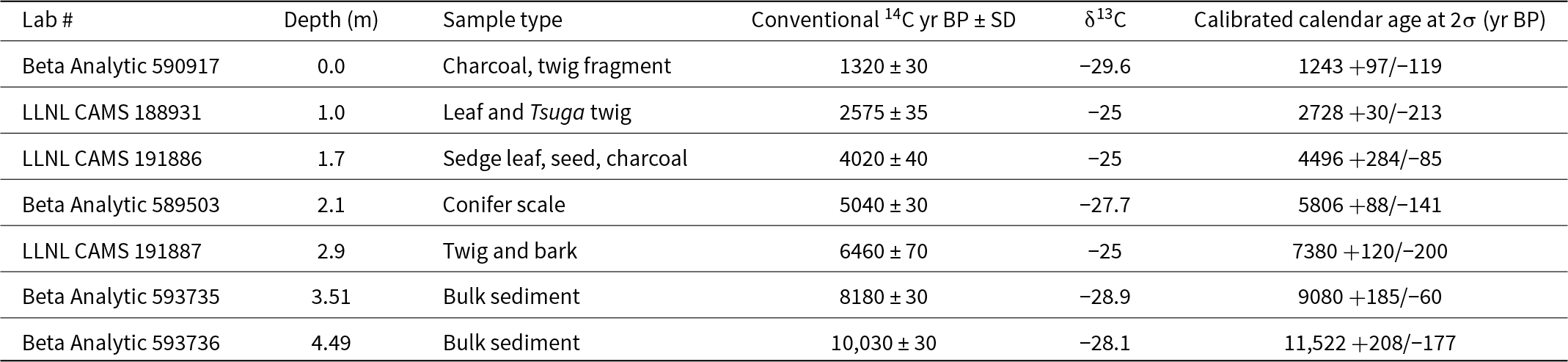
Table 2 Long description
Radiocarbon results are listed by lab number and core depth, with sample material, conventional radiocarbon age and uncertainty, carbon isotope value, and calibrated calendar age range. Ages generally get older with increasing depth, indicating a consistent age depth progression through the core. At 0.0 m, a charcoal twig fragment dates to about 1,320 years before present and calibrates to about 1,243 years with an uncertainty range. At 1.0 m, leaf and Tsuga twig material dates to about 2,575 years before present and calibrates to about 2,728 years, with an asymmetric uncertainty range. Mid core samples include sedge leaf, seed, and charcoal at 1.7 m dating to about 4,020 years before present and calibrating to about 4,496 years, and a conifer scale at 2.1 m dating to about 5,040 years before present and calibrating to about 5,806 years. Deeper samples include twig and bark at 2.9 m dating to about 6,460 years before present and calibrating to about 7,380 years, followed by bulk sediment at 3.51 m dating to about 8,180 years before present and calibrating to about 9,080 years. The deepest entry is bulk sediment at 4.49 m dating to about 10,030 years before present and calibrating to about 11,522 years. Carbon isotope values range from about minus 29.6 to minus 25, and calibrated ages and uncertainties depend on calibration and sample type, with bulk sediment potentially reflecting mixed carbon sources.
Pollen and macrofossil stratigraphy
As in the Dyken Pond core, the basal clastic sediments are devoid of pollen and plant macrofossils, so the record begins at 11,950 cal yr BP, near the bottom of the gyttja interval. We drew zone boundaries with the help of CONISS and emphasized similarities to the Dyken Pond record. Zone SP-1 (11,950–11,740 cal yr BP) begins with abundant Abies (>35%) and Pinus (>30%) pollen along with lesser amounts of Picea and Quercus pollen (Fig. 9). No macrofossils were recovered from this level (Fig. 10).
Pollen and spore stratigraphy of the Shaver Pond core. Sediments below 4.7 m are nearly devoid of organic matter and yielded insufficient pollen grains for analysis.

Figure 9 Long description
Shaver Pond Pollen and Spores A multi-column stratigraphy chart with many narrow plots aligned by depth. The left side shows two vertical scales: Depth (m) and Calendar Age (yr BP). Depth (m) is labeled from 0.0 to 4.5. Calendar Age (yr BP) is labeled from 1000 to 12000. Across the bottom, a shared label reads Percentage of Total Pollen. Individual taxa columns are labeled at the top, left to right: Pinus; Picea; Abies; Larix; Tsuga; Quercus; Fagus; Betula; Alnus; Acer; Corylus; Ostrya-Carpinus; Carya; Juglans; Ulmus; Populus; Tilia; Plantaceae; Ericaceae; Asteraceae; Cyperum; Sphagnum. Each taxa column contains a single filled line profile that varies with depth. Most columns show values concentrated near the left side of their small horizontal scale, with occasional wider bulges at specific depths. The Pinus column shows the widest profile overall, with a broad section in the lower part of the core and narrower sections toward the top. Several mid-sequence columns show moderate-width profiles at multiple depths, while many of the rightmost columns remain narrow for most depths. Horizontal dashed guide lines run across the plots at multiple depths. On the right, a column labeled Pollen Zones lists zone labels from bottom to top: SP-1, SP-2, SP-3, SP-4, SP-5, SP-6, SP-7, SP-8, SP-9. Adjacent to this is a dendrogram labeled CONISS. The dendrogram has a horizontal axis labeled Total sum of squares with tick labels 0, 20000, 40000 and 60000 and branching lines aligned with the listed zones. Small text near the lower right reads Analyst: Owczarek.
Macrofossils and charcoal found in the Shaver Pond core. No macrofossils were recovered below 4.5 m.

Figure 10 Long description
Shaver Pond Macrofossils. A multi-column stratigraphic chart with a shared vertical scale at left. The leftmost vertical axis is labeled Depth (m) with tick labels 0.0, 0.5, 1.0, 1.5, 2.0, 2.5, 3.0, 3.5, 4.0 and 4.5. A second vertical axis is labeled Calendar Age (yr BP) with tick labels 1000, 2000, 3000, 4000, 5000, 6000, 7000, 8000, 9000, 10000, 11000 and 12000. Horizontal dashed lines run across the tracks at multiple depths. Across the top, narrow tracks are labeled (left to right): Pinus strobus needle; Conifer needle scales; Conifer wing; Conifer seed; Tsuga needle; Bud scale; Betula lenta seed; Cirsi seed; Bryophyte stem leaves; Sphagnum; Typha seed; Isoetes; Cladoceran ephippia; Bryozoan statoblast; Insect parts; Mite; Charcoal. At the bottom center, the horizontal axis label reads Number per 25 cm superscript 3 of sediment. Most tracks show short horizontal marks at scattered depths. The Tsuga needle track includes a longer horizontal mark near depth about 1.8 m. The Cladoceran ephippia track contains multiple long horizontal bars between about 3.0 m and 4.5 m, with several bars extending to labeled values 20, 40, 60 and up to about 80 on its scale. The Insect parts track shows filled circular points at several depths, including a group between about 2.6 m and 3.1 m and another group between about 3.5 m and 4.1 m, plus additional points near about 1.9 m to 2.0 m and near about 4.4 m. At the far right, a column labeled Pollen Zones lists SP-9, SP-8, SP-7, SP-6, SP-5, SP-4, SP-3, SP-2 and SP-1 aligned to depth intervals.
Both Abies and Pinus pollen percentages decline precipitously as Alnus, Betula, and Picea expand in zone SP-2 (11,740–11,180 cal yr BP, Fig. 9). Larix rises at the same time. In the macrofossil record, the end of the zone is marked by the highest amount of charcoal throughout the entire sequence (Fig. 10).
In zone SP-3 (11,180–10,500 cal yr BP), Betula and Alnus pollen percentages both decline significantly and reach near minimum values for the entire record (Fig. 9). Pinus rapidly expands to its maximum value of 65%, and Picea experiences another small peak in abundance (∼5%), whereas Abies and Larix pollen effectively disappear. Quercus increases to ∼15% at the end of the zone, and Tsuga and Fagus percentages start to rise at zone end. Conifer needle scales and insect parts make their first appearance in the macrofossil record (Fig. 10). No charcoal was found.
Zone SP-4 (10,500–9100 cal yr BP) is marked by the decline of Pinus pollen to ∼40% of the sum along with a continuing rise in Tsuga, which constitutes 22% of the sum by zone end, when Pinus shows a small resurgence (Fig. 9). The interval also shows significant expansion in Quercus pollen (peak of ∼32%), followed by a decline in that taxon to ∼15% at zone end. Both Fagus and Tsuga show oscillations opposite to those shown by Quercus. Betula measures ∼5% of the sum at the beginning of the zone, and it, Picea, and Abies show small peaks in abundance mid-zone. In the macrofossil record, insect parts are found throughout the zone, and conifer needle scales appear in the middle and at the top of the zone (Fig. 10). Tsuga needles and charcoal appear about two thirds of the way up the zone.
Pinus pollen percentage continues its decline in zone SP-5 (9100–7960 cal yr BP) as Fagus, Betula, and Acer rise relative to their abundances in zone SP-4 (Fig. 9). Tsuga declines before recovering to approximately 30% of the sum by zone end, and Picea disappears from the record. Conifer needle scales are present mid-zone in the macrofossil record along with Sphagnum and Tsuga needles (Fig. 10). Insect parts are absent for most of the zone.
Zone SP-6 (7960–5300 cal yr BP) features major fluctuations in Tsuga pollen percentage that influence the other genera. The taxon, which had generally been increasing since the start of the zone, declines to about 15% of the pollen sum at 6170 cal yr BP and then rebounds past its previously highest value to reach a maximum of 37% at 5460 cal yr BP (Fig. 9). Leading into the Tsuga trough at 6170 cal yr BP, Alnus, and then Acer, peak and then decline as Tsuga recovers. Fagus (18%) and Betula (12%) also increase during the Tsuga trough, but lack distinct peaks. Quercus (5%) does not show much of an increase when Tsuga declines, but does strongly decrease toward the end of the Tsuga rebound. Once Tsuga has completed its recovery, Alnus (4%) and Fagus (19%) slightly increase, while the other deciduous genera show minima. Conifer needle scales and Tsuga needles are prevalent throughout the zone (Fig. 10), whereas insect parts disappear in the latter half of the zone.
Percentage of Lindavia rossii in the Shaver Pond core. We used this alkaliphilic taxon to determine when the hydrologic balance in the lake shifted toward greater contributions of alkaline groundwater, which would be expected during drier climate.

Figure 11 Long description
Shaver Pond. The horizontal axis at the top is labeled percent Lindavia rossii, with tick labels 0, 10, 20, 30, 40. The left vertical axis is labeled Depth (m), ranging from 0.0 to 4.5 with tick labels at 0.0, 0.5, 1.0, 1.5, 2.0, 2.5, 3.0, 3.5, 4.0, 4.5. A second vertical axis is labeled Calendar Age (yr BP), ranging from 1000 to 12,000 with tick labels at 1000, 2000, 3000, 4000, 5000, 6000, 7000, 8000, 9000, 10,000, 11,000, 12,000. A single line with circular markers is plotted. Most markers lie close to the 0 mark on the percent Lindavia rossii axis. A set of points between about 1.5 and 2.3 on the Depth (m) axis extends rightward to higher percent values, including one point near the 20 mark around Calendar Age 4000, one point near the 30 mark around Calendar Age 5000 and one point near the 40 mark around Calendar Age 6000. On the right side, a column is labeled Pollen zones. The labels shown from top to bottom are SP-9, SP-8, SP-7, SP-6, SP-5, SP-4, SP-3, SP-2, SP-1. Horizontal dashed lines separate the zones.
The well-known Mid-Holocene Tsuga collapse occurs in Zone SP-7 (5300–3200 cal yr BP) as that taxon abruptly declines from 37% to 5% of the pollen sum (Fig. 9). This collapse is met with increases in Quercus (30%) and Acer (16%) pollen, whose trends are in phase with one another and out of phase with Betula and Fagus. Alnus is slightly elevated at the onset of Tsuga collapse (4%) but then declines, Abies reappears but is less than 2% mid-collapse, and Pinus rises relative to zone SP-6, oscillating between 5% and 12% of the pollen sum. Tsuga needles are present throughout the zone, showing their greatest abundance at the time of peak collapse of the taxon in the pollen record (4800 cal yr BP, Fig. 10). Conifer needle scales are present in similar abundance to prior zones, and Betula lenta seeds appear at both the beginning and end of the zone (Fig. 10). Bryozoan statoblasts, present only once before in the Shaver Pond record, at the end of zone SP-5, reappear mid-zone and continue through the middle of zone SP-8 (ca. 2000 cal yr BP). Insect remains were found from 5140–4800 cal yr BP, but then disappear for the rest of the record.
At 3440 cal yr BP, Tsuga pollen percentage begins to rebound, which signals the onset of zone SP-8 (3200–1370 cal yr BP, Fig. 9). Tsuga rises to 25% and generally maintains this percentage, with the exception of a prominent decline at 2550 cal yr BP (∼10%) and another at the end of the zone at 1370 cal yr BP (∼8%), the latter of which coincides with small increases in Abies pollen (but less than 2%). Quercus shows broad fluctuations (5–15%) out of phase with similar, but lower amplitude, fluctuations in Pinus. Fagus and Betula show finer scale oscillations out of phase with one another, and Acer (7%) has a generally stable trend, with minor peaks during the Tsuga declines. In the macrofossil record, Tsuga needles are present throughout the zone, and conifer needle scales appear at various intervals.
Zone SP-9 commences at 1370 cal yr BP when Picea (2%) reappears in the pollen record and Tsuga again rebounds to ∼25% of the pollen sum (Fig. 9). Quercus, Betula, and Acer decline, while Fagus and Alnus expand slightly. Tsuga needles are present in the macrofossil record (Fig. 10).
Diatom stratigraphy
As in the case of Dyken Pond, the Late Pleistocene and Holocene diatom sequence at Shaver Pond contains more than 200 different species typical of low alkalinity lakes in the northeastern United States, with the vast majority found only in very small abundances and sporadically throughout the record (Menking et al., Reference Menking, Tipton and Bixby2026). Figure 11 shows the percentage of Lindavia rossii, which we discuss in the context of the pollen zones described above. The series starts at 11,740 cal yr BP (in pollen zone SP-2) due to lack of sufficient valves to enumerate below that depth. The percentage of L. rossii measures 0.7% before falling to 0% until 10,335 cal yr BP in zone SP-4, when the taxon reappears at 0.23% of the count. Thereafter, it again falls to 0%, where it remains until the end of zone SP-5 at ca. 7960 cal yr BP, where it constitutes ∼0.5%. Values return to zero before rising to 3.6% of the count at ca. 7200 cal yr BP (middle of zone SP-6). Percentages then drop to zero again before starting to climb at ca. 6170 cal yr BP and then undergoing large-amplitude oscillations between zero and as high as 36% until 3680 cal yr BP (second half of zone SP-6 through most of zone SP-7). Peaks in percentage occur at 5780 (36%), 5140 (27%), and 3970 (12%) cal yr BP before values drop to zero again. The diatom appears again in single samples at very low abundances (<1%) at 3440, 2390, 1660, and 1230 cal yr BP (end of zone SP-7 through zone SP-9).
Discussion
The radiocarbon date found at the base of the organic interval in the Dyken Pond core (Fig. 3, Table 1) indicates that parts of the Rensselaer Plateau have been ice free since at least 13,300 cal yr BP, a result consistent with nearby records in New York’s Catskill Mountains (Peteet et al., Reference Peteet, Ibe, Stone, Zajac and Chang2024) and Mohawk River Valley (Toney et al., Reference Toney, Rodbell and Miller2003) as well as in northwestern Massachusetts (Huvane and Whitehead, Reference Huvane and Whitehead1996). Sediment chemistry analyses (δ13C and C/N ratio) show the presence of an algal community in the sands, silts, and clays (Fig. 2) and that organic deposition began to increase significantly and changed to a mixture of C-3 plant and algal remains (Meyers, Reference Meyers1994), signifying forest arrival, around 13,040 cal yr BP. The Shaver Pond core shows a similar jump in the LOI proxy a little later at ca. 12,300 cal yr BP (Fig. 7). We note that this is an extrapolated age that could be too young given that we were unable to find datable material in the lowest ∼0.8 m of that core. Alternatively, the Shaver Pond record may have started later due to that site’s more northerly location and lower elevation. This could have favored continued ice cover for some period after the watershed surrounding Dyken Pond deglaciated, although there is some evidence from New York’s Catskill Mountains for lower-elevation sites becoming ice free earlier than higher-elevation sites (Peteet et al., Reference Peteet, Ibe, Stone, Zajac and Chang2024). In the sections presented below, we combine all of the data to explore the climate history of the Rensselaer Plateau over time and compare that history to other records from the Northeast. Figure 12 provides a summary of the dominant findings discussed in the text.
Climate summary for the Rensselaer Plateau. Numbers above peaks and troughs in the diatom and pollen time series are dates of events referenced in the text in cal kyr BP. AL refers to the Allerød warming and YD to the Younger Dryas. Colored bars represent different climate intervals based on the totality of the evidence (including macrofossils and diatoms). Selected drought records from the Middle Holocene (dark gray bars) and their relationship to the period of maximum Tsuga decline (gray bar) are also shown. Shawangunk Ridge from Menking et al. (Reference Menking, Peteet and Anderson2012), Blanding Lake and Sunfish Pond from Shuman et al. (Reference Shuman, Stefanova, Stefanescu, Ray-Cozzens, Johnson and Nelson2026), New Long Pond from Shuman et al. (Reference Shuman, Newby and Donnelly2009), and White Lake from Li et al. (Reference Li, Yu and Kodama2007).

Figure 12 Long description
The plot displays a stratigraphic time series with multiple panels showing the percentage of different taxa over age in calibrated kyr BP. The x-axis is labeled 'Age (cal kyr BP)' ranging from 14 to 0 and the y-axis is labeled 'Percentage' ranging from 0 to 15. The first panel shows Lindavia rossii with peaks at 5.14 and 7.2. The second panel displays Aulacoseira subarctica with peaks at 10.8 and 4.79. The third panel shows Pinus with a notable peak labeled 'YD' and a decline towards the present. The fourth panel displays Picea with peaks at 12.3 and 6.3. The fifth panel shows Tsuga with peaks at 13.0 and 2.3. A climate summary bar overlays the panels, indicating intervals such as 'cold and wet', 'cold and dry', 'warm and wet' and 'warm and dry'. Regional droughts during the middle Holocene are marked with dark gray bars. Specific events like the Allerød warming (AL) and Younger Dryas (YD) are annotated. The plot includes references to sites like Shawangunk Ridge, Blanding Lake and White Lake, indicating regional climate records.
Deglaciation and late Pleistocene forest arrival (>12,660 cal yr BP)
Zone DP-1 consists of a single sample, dating to 13,040 cal yr BP, that appears to reflect the Allerød interstade (Deevey, Reference Deevey1939). Thermophilous deciduous genera such as Quercus and Fagus were present in the pollen record (Fig. 4) along with Tsuga and small percentages of the boreal conifers Picea, Abies, and Larix. Somewhat surprising is the high percentage of Tsuga pollen, constituting more than 15% of the total sum (Fig. 4). Many records from the Northeast do not extend this far back in time, and those that do show the interstadial typically contains much lower percentages (Overpeck, Reference Overpeck1985; Peteet et al., Reference Peteet, Daniels, Heusser, Vogel, Southon and Nelson1993; Menking et al., Reference Menking, Peteet and Anderson2012). The very low organic matter (Fig. 2) and lack of Tsuga macrofossils (Fig. 5) at this level in the Dyken Pond core suggest that the pollen may have come from some distance away, although the influx data (see Supplementary Figure 1) show values as high as those during much of the Holocene. We note that Niles Huyck Bog in the nearby Catskill Mountains (Fig. 1) shows Tsuga percentages as high as 10% during a period at the base of that record that also contains up to 20% Picea, 10% Abies, and 20% Pinus (Ibe, Reference Ibe2017). There is no age control on that period, but based on comparison of the Pinus record to those throughout the region, this high Tsuga percentage appears to have occurred at the same time as that in Dyken Pond. Another site with high Tsuga during the Allerød interstadial is Balsam Lake, also in the Catskills (Fig. 1; Ibe, Reference Ibe1985), where percentages reach as high as 25%, along with abundant Pinus, Quercus, and Betula. The overall picture painted by the Dyken Pond pollen results thus suggests a climate that was warm enough to support Tsuga and Quercus.
Latest Pleistocene and Younger Dryas cooling (ca. 12,660–11,100 cal yr BP)
Both Dyken and Shaver ponds show unusually high percentages of Abies pollen (30–40%) immediately after the presumed Allerød interstadial. While many nearby records contain much lower percentages (for example, ∼8% at North Pond, MA, Huvane and Whitehead, 1986; ∼5% at Maplecrest Fen, NY, Peteet et al., Reference Peteet, Ibe, Stone, Zajac and Chang2024; <5% at Heart Lake and Upper Wallface Ponds, NY, Whitehead and Jackson, Reference Whitehead and Jackson1990; locations shown in Fig. 1), Toney et al. (Reference Toney, Rodbell and Miller2003) found values as high as 20% at Ballston Lake, immediately west of the Rensselaer Plateau. Similarly, Ibe (Reference Ibe1985, Reference Ibe2017) found values as high as 20–25% at Balsam Lake and Niles Huyck Bog in the Catskill Mountains (Fig. 1), southwest of our study sites, so higher percentages are not unprecedented. The Plateau is known to host stands of Abies balsamea today, in both forested uplands and wetlands, befitting its higher elevation than the nearby Hudson River Valley and colder climate (https://www.rensselaerplateau.com/about-the-plateau-c1ulz, accessed May 23, 2025). As such, the high Abies count seems in line with the cold and relatively wet conditions of the Late Pleistocene.
Peaks in Betula and Alnus pollen are noted at around 11,500 cal yr BP (Figs. 4 and 9) and have been associated with the Younger Dryas climate reversal (Peteet et al., Reference Peteet, Vogel, Nelson, Southon, Nickmann and Heusser1990, Reference Peteet, Daniels, Heusser, Vogel, Southon and Nelson1993; Levesque et al., Reference Levesque, Mayle, Walker and Cwynar1993; Mayle et al., Reference Mayle, Levesque and Cwynar1993; Oswald et al., Reference Oswald, Faison, Foster, Doughty, Hall and Hansen2007). These peaks are accompanied by increases in Picea and Larix pollen as well as by decreases in Tsuga and Quercus. Picea, Abies, and Larix macrofossils in the Dyken Pond core (Fig. 5) indicate locally cold temperatures (Peteet et al., Reference Peteet, Ibe, Stone, Zajac and Chang2024), a finding that may explain a spike in the percentage of A. subarctica at Dyken Pond (Fig. 6).
Peteet et al. (Reference Peteet, Daniels, Heusser, Vogel, Southon and Nelson1993) noted that the 3–4°C temperature drop associated with the Younger Dryas stade would have killed off Quercus and any Pinus strobus populations that had already become established in the Northeast, allowing replacement by taxa such as Alnus and Betula, and indeed, there are marked declines in Pinus pollen in both the Dyken and Shaver Pond records at this time (Figs. 4 and 9). The presence of Alnus signals moisture, and the interpretation of a cold and wet Younger Dryas stade on the Rensselaer Plateau (Fig. 12) agrees with findings from New York’s Finger Lakes (Mullins, Reference Mullins1998), lakes Mohonk and Minnewaska on the Shawangunk Ridge (Fig. 1; Menking et al., Reference Menking, Peteet and Anderson2012), Maplecrest Fen in New York’s Catskill Mountains (Fig. 1; Peteet et al., Reference Peteet, Ibe, Stone, Zajac and Chang2024), and Upper Wallface Pond, Heart Lake, and Brandreth Bog in the Adirondacks (Stefanescu et al., Reference Stefanescu, Shuman, Grigg, Bailey, Stefanova and Oswald2023) but is opposite to evidence from Sluice, Davis, Rocky, and New Long Ponds in Massachusetts (Fig. 1), which experienced lake lowstands between 13,400 and 10,900 cal yr BP (Newby et al., Reference Newby, Donnelly, Shuman and MacDonald2009, Reference Newby, Shuman, Donnelly and MacDonald2011; Hubeny et al., Reference Hubeny, McCarthy, Lewis, Drljepan, Morissette, King, Cantwell, Hudson and Crispo2015).
Early Holocene climatic variability (ca. 11,100–7500 cal yr BP)
Major declines in Alnus, Betula, and boreal conifer pollen, along with expansion of Tsuga and Quercus from ca. 11,100–10,090 cal yr BP (Figs. 4 and 9), herald the onset of Early Holocene warmth on the Rensselaer Plateau. This time interval also marks the highest percentage of Pinus pollen in both records, with conifer needle scales and Pinus strobus needles appearing at Dyken Pond (Fig. 5). As such, this period seems to correspond to the northeastern B-zone first identified by Deevey (Reference Deevey1939), a time of warm and dry conditions across the US Northeast (Davis, Reference Davis1969; Peteet et al., Reference Peteet, Daniels, Heusser, Vogel, Southon and Nelson1993, Reference Peteet, Ibe, Stone, Zajac and Chang2024; Robinson et al., Reference Robinson, Burney and Burney2005; Oswald et al., Reference Oswald, Faison, Foster, Doughty, Hall and Hansen2007; Menking et al., Reference Menking, Peteet and Anderson2012; Grigg et al., Reference Grigg, Stefanescu, Shuman and Oswald2023). Climate reconstructions based on pollen records and stable isotopes from sites throughout the region indicate as much as a 25% decrease in precipitation relative to the Middle Holocene (Webb et al., Reference Webb, Anderson and Webb1993), and temperatures 4–8°C warmer than in the Younger Dryas (Hou et al., Reference Hou, Huang, Oswald, Foster and Shuman2007; Grigg et al., Reference Grigg, Stefanescu, Shuman and Oswald2023).
The Dyken Pond diatom record shows a drop in percentage of A. subarctica relative to the end of the Younger Dryas stade (YD) at this time (Fig. 6), consistent with warmer conditions, interrupted by a small increase at 10,700 cal yr BP that might reflect a brief cooling. We expected to see an increase in the percentage of the alkaliphilic L. rossii at Shaver Pond during this warm interval, as drier conditions should have shifted the hydrologic balance toward greater importance of groundwater, but it appears that the acidifying effect of Pinus expansion (Brand et al., Reference Brand, Kehoe and Connors1986) prevented this from happening (Fig. 11). Additional evidence for climatic drying during the B-zone interval includes the first appearance of bryozoan statoblasts at Dyken Pond, suggesting lake levels were declining (Fig. 5). No similar appearance of statoblasts was found at Shaver Pond, but this may reflect differences in the bathymetry of the two waterbodies (Fig. 1).
At the end of the B-zone interval in the pollen record, both ponds show the onset of a major decline in Pinus pollen percentage as well as increased prominence of Quercus and Tsuga (Figs. 4 and 9). Dyken Pond experienced a step increase in Tsuga pollen at around 10,100 cal yr BP whereas Shaver showed a more gradual increase, beginning around 10,400 cal yr BP (Figs. 4, 9, 12). The replacement of Pinus by Tsuga suggests increasing moisture (Deevey, Reference Deevey1939; Shuman et al., Reference Shuman, Newby, Huang and Webb2004; Oswald et al., Reference Oswald, Faison, Foster, Doughty, Hall and Hansen2007). That the timing is somewhat different between the two lakes may be related to errors in chronology or to successional dynamics in the different forest compositions surrounding the two lakes.
While the pollen changes indicate warmth and greater moisture, multiple proxies show that climate oscillated between warmer and cooler and moister and drier for the next 2000 years. At 9900 cal yr BP, for example, a sudden increase in Sphagnum macrofossils and major expansion of oogonia of Chara in Dyken Pond (Fig. 5) suggest that lake level again declined. Mosses are sometimes pioneer species as lakes recede (Tsyganov et al., Reference Tsyganov, Kupriyanov, Babeshko, Borisova, Chernyshov, Volkova, Chekova, Mazei and Novenko2019), and charophytic algae generally prefer alkaline conditions and suggest greater importance of groundwater (Rey-Boissezon and Joye, Reference Rey-Boissezon and Joye2015; Peteet et al., Reference Peteet, Ibe, Stone, Zajac and Chang2024). Similarly, a decline in Tsuga centered around 9600 cal yr BP in the Shaver Pond record (Fig. 9) is matched by a decline in LOI (Fig. 7), which suggests greater oxidation of organic sediments produced by drier climate, as also occurred on the Shawangunk Ridge at this time (Menking et al., Reference Menking, Peteet and Anderson2012). Additional evidence of climatic variability includes high concentrations of Najas seeds, bryozoan statoblasts, and Potamogeton seeds at 9360 cal yr BP in the Dyken Pond record, suggesting low lake levels even as climate was generally becoming moister and capable of supporting Tsuga (Haas and McAndrews, Reference Haas, McAndrews and McManus2000; Peteet et al., Reference Peteet, Ibe, Stone, Zajac and Chang2024). These changes on the Rensselaer Plateau occurred contemporaneously with an approximately 1000-year-long interval of low moisture and warmer than modern temperatures at Twin Ponds in Vermont (Grigg et al., Reference Grigg, Stefanescu, Shuman and Oswald2023; Fig. 1).
In addition to rapidly changing moisture regimes, sub-millennial oscillations in temperature appear to have occurred after the B-zone pollen period. For example, around 9200 cal yr BP, Picea pollen and Picea seeds and Larix needles increased at Dyken Pond, signaling cooling. The Dyken record also shows a small increase in percentage of A. subarctica at this time (Fig. 6), and may reflect the 9200 cal yr BP event seen in records throughout the northern hemisphere when meltwater discharge from the retreating Laurentide ice sheet is thought to have initiated a slowdown in the Atlantic Meridional Overturning Circulation (AMOC) and cooling of the North Atlantic region (Fleitmann et al., Reference Fleitmann, Mudelsee, Burns, Bradley, Kramers and Matter2008; Hou et al., Reference Hou, Huang, Shuman, Oswald and Foster2011; Gao et al., Reference Gao, Huang, Shuman, Oswald and Foster2017; Couette et al., Reference Couette, Ghienne, Lajeunesse and van der Woerd2023).
Conditions after 9200 cal yr BP appear to have become warmer and much more mesic, reflected in major expansions in Tsuga and then Fagus pollen percentage (Shuman et al., Reference Shuman, Newby, Huang and Webb2004; Oswald et al., Reference Oswald, Faison, Foster, Doughty, Hall and Hansen2007), as well as further decline of Pinus (Figs. 4 and 9). Tsuga needles and seeds and a variety of Betula papyrifera and B. lenta macrofossils accompanied these palynological changes at Dyken Pond, signaling moist climate, as did declines in the quantities of Najas seeds, oogonia of Chara, and bryozoan statoblasts (Fig. 5), suggesting higher lake levels. Still, a single large increase in oogonia of Chara in Dyken Pond at 8150 cal yr BP (Fig. 5), along with small increases in bryozoan statoblasts in both the Dyken and Shaver (Fig. 10) records, suggests transitory drier conditions within this otherwise wetter period.
In the pollen record, Tsuga percentage declined at ca. 8200 cal yr BP at Dyken Pond and a little earlier (ca. 8600 cal yr BP) in Shaver Pond (Fig. 12). Huvane and Whitehead (Reference Huvane and Whitehead1996) found a Tsuga pollen decline at ca. 8200 cal yr BP (reported as 7500 14C yr BP) at North Pond in western Massachusetts (Fig. 1) that was associated with an increase in charcoal and a brief increase in benthic diatoms that was attributed to a transient drought associated with increased warmth. At Dyken Pond, however, a slight increase in Larix pollen (Fig. 4) and a small increase in the percentage of A. subarctica (Fig. 6) occurred at this time, suggesting a slight cooling in eastern New York that comports with other studies across New England that correlated the 8200 cal yr BP event to release of meltwater from the Laurentide ice sheet and disruption of the AMOC (Hou et al., Reference Hou, Huang, Wang, Shuman, Oswald, Faison and Foster2006; Shuman et al., Reference Shuman, Huang, Newby and Wang2006, Reference Shuman, Newby and Donnelly2009; Shuman, Reference Shuman2012). The rapid recovery of Tsuga and expansion of Fagus after the event (Figs. 4 and 9) indicate that climate on the Rensselaer Plateau shifted back to warmer and wetter conditions thereafter.
The centennial- to sub-millennial-scale climate oscillations seen on the Plateau during the Early Holocene are consistent with similar variability reported for Blood Pond and Little Pond in Massachusetts (Fig. 1). Depleted deuterium isotope excursions in leaf waxes at Blood Pond were used to infer cooling episodes at 10,600, 10,200, 9500, 9200, 8800, and 8400 cal yr BP that may have been related to meltwater releases from the retreating Laurentide ice sheet and consequent effects on the AMOC (Hou et al., Reference Hou, Huang, Shuman, Oswald and Foster2011). The Little Pond record shows similar excursions at 10,700, 10,200, 9800, 9400, 9200, 8900, 8500, and 8200 cal yr BP and an association between colder temperatures and drier climate prior to 6250 cal yr BP (Gao et al., Reference Gao, Huang, Shuman, Oswald and Foster2017). Many of these episodes appear to show increases in the percentage of A. subarctica at Dyken Pond (Fig. 12). Higher resolution sampling, additional age control, and inclusion of stable isotopes will be necessary to confirm whether the palynologic, macrofossil, and diatom excursions on the Rensselaer Plateau align precisely with the Massachusetts records.
Middle Holocene Tsuga expansion (ca. 7500–5500 cal yr BP)
By ca. 7500 cal yr BP, Pinus pollen dropped to its lowest percentage in both the Dyken and Shaver Pond records (Figs. 4 and 9) as Tsuga and Fagus percentages continued to expand, signifying overall wetter conditions (Oswald et al., Reference Oswald, Faison, Foster, Doughty, Hall and Hansen2007; Peteet et al., Reference Peteet, Ibe, Stone, Zajac and Chang2024). In both lakes, Quercus pollen declined slightly throughout the next 2000-year interval and underwent opposite fluctuations in abundance to Fagus. An increase in the percentage of the alkaliphilic L. rossii at ca. 7200 cal yr BP in the Shaver Pond record (Fig. 11) roughly correlates with a decline in Tsuga pollen percentage in both ponds, rise in Quercus (Fig. 9) at Shaver, and decline in LOI (Fig. 7) at Shaver, and suggests a period of modestly drier climate that shifted the hydrologic balance toward greater importance of alkaline groundwater. No evidence of lake level decline occurs in the macrofossils of either record, so the dry interval may have been brief or minor. We note, however, that Newby et al. (Reference Newby, Donnelly, Shuman and MacDonald2009) identified lake lowstands in New Long Pond and Rocky Pond (Fig. 1) at this same time, and Hou et al. (Reference Hou, Wu, Cohen, Zeng, Huang, Zheng and Ge2023) presented evidence for a 7200 cal yr BP event in 58 different proxy records distributed across the globe.
A much larger decline in Tsuga pollen at ca. 6170 cal yr BP in Shaver Pond (Fig. 9) and a more subtle drop centered around ca. 6130 cal yr BP in Dyken Pond (Fig. 4) occurred at roughly the same time as a similarly timed decline in Tsuga pollen at Knob Hill Pond, Vermont (Fig. 1) that Oswald and Foster (Reference Oswald and Foster2011) hypothesized was caused by drought. A small increase in the percentage of A. subarctica at Dyken Pond (Fig. 6) accompanies the Rensselaer Plateau Tsuga declines and suggests minor cooling. This cooling appears to correlate with the first (6100 cal yr BP) of several Middle and Late Holocene cooling and drying episodes recognized in White Lake, New Jersey (Li et al., Reference Li, Yu and Kodama2007), but there is no evidence of drying in the macrofossil or diatom records of either Rensselaer Plateau lake until ca. 5800 cal yr BP, when the percentage of L. rossii shows the first of three prominent spikes in the Shaver Pond record. We note that Gao et al. (Reference Gao, Huang, Shuman, Oswald and Foster2017) found a correlation between cool and wet conditions and warm and dry conditions after 6250 cal yr BP at Little Pond, Massachusetts, opposite to their findings in the Late Pleistocene and Early Holocene and opposite to the findings for White Lake. Given that Dyken and Shaver ponds are close in latitude to Little Pond but more than 250 km north of White Lake, the ca. 6150 cal yr BP Tsuga decline on the Rensselaer Plateau may have been a response more to a drop in temperature than to a change in moisture.
Whatever the cause, after the event at ca. 6150 cal yr BP, Tsuga pollen percentage again increased, peaking in both records at ca. 5500 cal yr BP (Figs. 4 and 9), a finding mirrored in the macrofossils at Dyken Pond, where that taxon’s needles increased in concentration (Fig. 5). Conditions appear to have been among the wettest in the entire Holocene (Fig. 12), consistent with findings from New England (Shuman et al., Reference Shuman, Newby, Huang and Webb2004). In central New York, Lake Cayuga showed a highstand, although it was only about half as high as one that occurred earlier in the Holocene (Mullins, Reference Mullins1998); lake levels were declining at Lake Owasco at the same time (Dwyer et al., Reference Dwyer, Mullins and Good1996).
Mid-Holocene Tsuga decline and recovery (ca. 5460–3200 cal yr BP)
The classical Mid-Holocene Tsuga pollen decline seen throughout the Northeast immediately followed the peak in that taxon’s abundance and commenced at approximately 5460 cal yr BP in both Rensselaer Plateau records (Figs. 4 and 9). Percentages remained low in Dyken Pond until about 3800 cal yr BP and in Shaver until about 3500 cal yr BP (Fig. 12). In the macrofossil records (Figs. 5 and 10), Tsuga needle abundances generally mirrored the declines in pollen, dropping out of the record, although there was a major increase in needle deposition at Shaver Pond at ca. 4790 cal yr BP in the midst of the pollen decline and prior to disappearance of the taxon from the macrofossils. Menking et al. (Reference Menking, Peteet and Anderson2012) interpreted a similarly timed spike in Tsuga branchlet abundance in Lake Minnewaska on southeastern New York’s Shawangunk Ridge (Fig. 1) as indicating total collapse of that taxon and influx of macrofossils into the lake. Why Dyken Pond did not experience the same degree of Tsuga macrofossil influx as Shaver Pond may be related to the heterogeneity of the forests on the Rensselaer Plateau mentioned in the study setting. Dyken Pond is surrounded today by beech–maple mesic forest, whereas the Shaver Pond watershed includes a mix of beech–-maple mesic forest and hemlock–northern hardwood forest. As such, there may simply have been fewer Tsuga trees present around Dyken Pond at the time of the collapse, leading to a less sensitive macrofossil record.
Increased concentrations of bryozoan statoblasts at Shaver Pond (Fig. 10) during much of the period of the Tsuga decline suggest lower lake levels and therefore drought as a potential cause of the collapse, an inference bolstered by the pond’s diatom record, where the period during the decline is marked by two additional peaks in percentage of L. rossii centered around 5140 and 3970 cal yr BP (Figs. 11 and 12). Although drought appears to have been an important driver, declining temperature may also have played a role in the Tsuga decline, with the percentage of A. subarctica in Dyken Pond showing peaks centered at 4790, 4210, and 3420 cal yr BP (Figs. 6 and 12). The first of these peaks coincides with the time of greatest Tsuga needle concentration in the Shaver Pond record (Fig. 10), and the second precedes a small increase in Picea pollen (Fig. 4) and Picea needles (Fig. 5) at Dyken and Abies pollen at Shaver (Fig. 9) by about 200 years, all of which occurred while the percentage of A. subarctica was still modestly elevated. It is worth noting that Li et al. (Reference Li, Yu and Kodama2007) identified a cool drought interval in White Lake, New Jersey, at 4400 cal yr BP that might correlate to the 4210 cal yr BP cooling indicated by the percentage of A. subarctica at Dyken Pond. Conversely, Grigg et al. (Reference Grigg, Stefanescu, Shuman and Oswald2023) found evidence for moister climate along with a cooling of 0.75–1°C at Knob Hill Pond and Twin Ponds in Vermont (Fig. 1) at this time.
The rapid alternation of warm/cool and dry/wet conditions throughout the period of Tsuga decline suggests a sort of climate whiplash that appears to have been detrimental to the taxon. Shuman et al. (Reference Shuman, Stefanova, Stefanescu, Ray-Cozzens, Johnson and Nelson2026) discussed similar findings in two records from Pennsylvania: Sunfish Pond (Fig. 1), where the Tsuga decline followed lake level lowering that commenced at 5800 cal yr BP and ended by 3800 cal yr BP, and Blanding Lake (Fig. 1), where the decline followed lake level lowering that extended from 5500–3800 cal yr BP. We note that the 5800 cal yr BP starting date for lake level decline at Sunfish matches well the percent L. rossii peak in the Shaver Pond record that preceded the Tsuga decline on the Rensselaer Plateau (Fig. 12). A combination of stable isotopes and pollen analyses on Grinnell Lake in northern New Jersey (Fig. 1) also shows that Tsuga decline followed a climate shift at 5800 cal yr BP, lagging that shift by 350–500 years (Zhao et al., Reference Zhao, Yu, Ito and Zhao2010). The Pennsylvania records further include organic biomarkers sensitive to temperature changes that show that rapid warming of 0.9–1.3°C between 5150 and 4880 cal yr BP accompanied the Tsuga decline (Shuman et al., Reference Shuman, Stefanova, Stefanescu, Ray-Cozzens, Johnson and Nelson2026). This is similar in timing to the warm drought that appears to have hit the Rensselaer Plateau around the time of the 5140 cal yr BP percentage L. rossii peak, and we note that the diatoms in Shaver Pond suggest a return to cool and moist conditions at 4800 cal yr BP. Two additional warm/cool oscillations (% A. subarctica) on the Rensselaer Plateau coincide with only one additional wet/dry oscillation (% L. rossii), suggesting that drought conditions coincided with both warm and cool conditions between 4500 and 3600 cal yr BP (Fig. 12), something also true of Sunfish Pond (Shuman et al., Reference Shuman, Stefanova, Stefanescu, Ray-Cozzens, Johnson and Nelson2026), although the timing is different between the two sites.
While the diatom record on the Rensselaer Plateau implicates both cooler temperatures and warm and cool droughts in the Tsuga decline, other studies suggest only warmth along with dry conditions. At Maplecrest Fen, for example, Betula lutea macrofossils were present during the Tsuga decline (Peteet et al., Reference Peteet, Ibe, Stone, Zajac and Chang2024). Betula lutea has very similar temperature tolerances to Tsuga canadensis (Thompson et al., Reference Thompson, Anderson, Pelltier, Strickland, Shafer, Bartlein and McFadden2015), suggesting that temperatures didn’t necessarily change at that site. Similarly, at lakes Mohonk and Minnewaska on the Shawangunk Ridge, Pinus rigida needles appeared in the macrofossil record during the period of Tsuga decline (Menking et al., Reference Menking, Peteet and Anderson2012). Pinus rigida prefers warmer winter and summer temperatures and drier climate than does Tsuga canadensis (Thompson et al., Reference Thompson, Anderson, Pelltier, Strickland, Shafer, Bartlein and McFadden2015).
Conversely, evidence for cool droughts being responsible for the Tsuga decline are interpreted from changes in New Long Pond, Massachusetts, where such episodes appear to have occurred from 6300–6000 cal yr BP, 4700–4600 cal yr BP, and 3700–3300 cal yr BP (Shuman et al., Reference Shuman, Newby and Donnelly2009; Fig. 12). As with the Shawangunk Ridge (Menking et al., Reference Menking, Peteet and Anderson2012), the Rensselaer Plateau lies intermediate in longitude between this coastal Massachusetts site and north-central Pennsylvania, and therefore might be expected to show variable associations over time. The synoptic climatology that led to regional variations in temperature and moisture during the Middle Holocene requires additional study.
Interestingly, while episodes of drier climate are implicated in the Tsuga decline on the Rensselaer Plateau, no increase in charcoal was observed in the record from either pond, a result consistent with findings at North Pond, Massachusetts. Huvane and Whitehead (Reference Huvane and Whitehead1996) interpreted the lack of charcoal at that site to mean that the cause of the decline was some kind of insect pest or pathogen—an idea first proposed by Davis (Reference Davis, Bharadwaj, Vishnu-Mittre and Maheshwari1981) and later expanded upon by Bhiry and Filion (Reference Bhiry and Filion1996), who attributed the mortality of Tsuga in southern Quebec to an outbreak of the lepidopteran hemlock looper (Lambdina fiscellaria) after studying macrofossils of both insect remains and insect-chewed Tsuga needles. A massive increase in insect parts in the Dyken Pond macrofossil record (Fig. 5) just prior to the Tsuga collapse is tantalizing, but we have not yet been able to identify those remains in order to determine whether they came from species with known negative associations to Tsuga. We further note that Oswald et al. (Reference Oswald, Doughty, Foster, Shuman and Wagner2017) found no evidence of hemlock looper in a Tsuga-dominated forest in north-central Massachusetts that nevertheless showed the classical pollen decline and therefore concluded that insects were not the primary cause.
Together, the diatom, plant macrofossil, and pollen evidence from the Rensselaer Plateau suggests that a prolonged period unfavorable to Tsuga and punctuated by a series of climatic cooling events and droughts, between which the trees could not recover, played a major role in the Mid-Holocene Tsuga decline. Whether an insect pest or other pathogen was also involved remains an open question but seems unlikely to have been the primary driver of the decline given that the shallow roots (<20 cm depth) of Tsuga seedlings and saplings makes them very vulnerable to drought, thereby ensuring that the species would have been unable to reproduce except in moist refugia such as ravines and north-facing slopes (Miller, Reference Miller1973; Haas and McAndrews, Reference Haas, McAndrews and McManus2000).
By ca. 3300 cal yr BP, climate on the Rensselaer Plateau ameliorated, and increasing Tsuga pollen percentages (Figs. 4 and 9) show the taxon was well on its way to recovery, although, as in most records from the Northeast (Haas and McAndrews, Reference Haas, McAndrews and McManus2000; Menking et al., Reference Menking, Peteet and Anderson2012), it never regained its former prominence. The timing of the recovery matches well those from Sunfish Pond and Blanding Lake in Pennsylvania as well as a record from Ballston Lake, just west of the Plateau (Toney et al., Reference Toney, Rodbell and Miller2003), although Shuman et al. (Reference Shuman, Newby and Donnelly2009) found that full recovery in parts of New England was delayed until as late as 2000 cal yr BP.
Late Holocene wetter conditions (ca. 3200-ca. 1950 cal yr BP)
Wetter conditions prevailed on the Rensselaer Plateau in the Late Holocene. Tsuga and Fagus pollen were abundant in both records while Quercus declined (Figs. 4 and 9), and Tsuga needles became common again in the macrofossil records of both lakes (Fig. 5 and 10). In the diatom record, the percentage of A. subarctica dropped to zero at Dyken Pond (Fig. 6), and the abundance of L. rossii declined at Shaver Pond (Fig. 11), signaling warm and wet conditions. In the broader region, Shuman et al. (Reference Shuman, Newby, Huang and Webb2004) noted that the climate of the past 3000 years was likely wetter in New England than at any other time since deglaciation. This assertion is based on transgressive lacustrine sediments dating as far back as that time, but not earlier, in locations such as Crooked Pond and Makepeace Cedar Swamp in Massachusetts as well as at Echo Lake in New Hampshire (Fig. 1). In contrast, falling lake levels prevailed in Cayuga Lake in central New York from ca. 4400 cal yr BP to the present, which Mullins et al. (Reference Mullins, Patterson, Teece and Burnett2011) attributed to a cooler and drier climate than during the Middle Holocene.
Late Holocene cooling (ca. 1370 cal yr BP to present)
Picea pollen expanded in the Shaver Pond record at ca. 1370 cal yr BP, signifying cooling, simultaneous with an abrupt decline in Tsuga pollen percentage at that site and similar in timing to a cool drought interval (1300 cal yr BP) at White Lake, New Jersey (Li et al., Reference Li, Yu and Kodama2007). A rise in Picea percentage at Dyken Pond occurred somewhat later (ca. 800 cal yr BP). The percentage of A. subarctica at Dyken Pond suggests warm conditions from ca. 2930 cal yr BP (Fig. 6) all the way up to ca. 1080 cal yr BP (Fig. 6), followed by a transitory cool episode when this taxon briefly increased in abundance. The diatom record notwithstanding, cooler conditions may have prevailed in the Dyken watershed from ca. 1080 cal yr BP onward given the reappearance of Picea and Larix needles in the Dyken macrofossil record (Fig. 5).
Regionally, the timing of neoglacial cooling is quite variable. At Brandreth Bog in the Adirondack Mountains of New York (Fig. 1), for example, Overpeck (Reference Overpeck1985) found that Picea and Abies began to increase at the expense of more temperate taxa around 4450 cal yr BP (reported as 4000 14C yr BP) whereas other sites in the Adirondacks show an increase in Picea beginning around 3170 cal yr BP (reported as 3000 14C yr BP; Jackson and Whitehead, Reference Jackson and Whitehead1991). At Maplecrest Fen in the Catskills, Picea pollen began to rise at 2700 cal yr BP (Peteet et al., Reference Peteet, Ibe, Stone, Zajac and Chang2024); at Ballston Lake, increases in Picea and Betula signal cooling beginning around 2400 cal yr BP; at Crooked Pond in eastern Massachusetts, cooling began around 3000 cal yr BP (Shuman et al., Reference Shuman, Newby, Huang and Webb2004); and at Spruce Pond in New York’s Hudson Highlands, Picea began to rise at 1350 cal yr BP (reported as 1470 14C yr BP; Maenza-Gmelch, Reference Maenza-Gmelch1997). The great diversity of vegetation communities on the Rensselaer Plateau may be responsible for the variability in timing of cooling between Dyken and Shaver Ponds if taxa such as Picea, Larix, and Abies were present in isolated refugia closer to one lake than another.
Additional notable features in the Dyken Pond pollen record include large increases in Sphagnum spores and Asteraceae pollen (primarily Ambrosia) around 560 cal yr BP (Fig. 4), the latter of which is almost certainly related to European settlement, given errors in age control (Davis, Reference Davis1969; Maenza-Gmelch, Reference Maenza-Gmelch1997; Pederson et al., Reference Pederson, Peteet, Kurdyla and Guilderson2005). Sphagnum macrofossils and bryozoan statoblasts also increased at this time, suggesting the lake may have become more shallow. The percentage of organic carbon fell simultaneously (Fig. 2), which could have been related to increased soil erosion and mineral input associated with European watershed disturbances that would in turn have led to lake shallowing, but we note that there is no evidence in the diatom record to support this supposition (Menking et al., Reference Menking, Tipton and Bixby2026). As such, the decline in organic carbon content may simply be related to the increase in coniferous taxa (Pinus, Picea, and Larix), with their slow rates of needle loss, at the expense of deciduous taxa (particularly Fagus and Betula; Fig. 4).
Conclusions
Pollen records from the Rensselaer Plateau show broad similarity to the classical northeastern vegetation zones first identified by Deevey (Reference Deevey1939) and later confirmed by Davis (Reference Davis1969) and a host of other studies within the region (Ibe, Reference Ibe1985, Reference Ibe2017; Peteet et al., Reference Peteet, Vogel, Nelson, Southon, Nickmann and Heusser1990, Reference Peteet, Daniels, Heusser, Vogel, Southon and Nelson1993, Reference Peteet, Ibe, Stone, Zajac and Chang2024; Toney et al., Reference Toney, Rodbell and Miller2003; Shuman et al., Reference Shuman, Newby, Huang and Webb2004; Robinson et al., Reference Robinson, Burney and Burney2005; Menking et al., Reference Menking, Peteet and Anderson2012). These include (1) a mixed thermophilous–boreal forest assemblage containing Abies, Picea, and Larix pollen along with Pinus, Quercus, and Tsuga at or near the base of some records; (2) an overlying drop in Pinus and expansion of Picea, and particularly Alnus and Betula, signifying the Younger Dryas climatic reversal (Levesque et al., Reference Levesque, Mayle, Walker and Cwynar1993; Peteet et al., Reference Peteet, Vogel, Nelson, Southon, Nickmann and Heusser1990, Reference Peteet, Daniels, Heusser, Vogel, Southon and Nelson1993); (3) a subsequent decline of boreal taxa with expansion of Pinus (most likely P. strobus) to its highest abundance, associated with Early Holocene warming and drying (Deevey, Reference Deevey1939; Shuman and Marsicek, Reference Shuman and Marsicek2016; Oswald et al., Reference Oswald, Foster, Goodell and Shuman2023); and then (4) a decline in that taxon as Tsuga, Quercus, and Fagus rose to prominence, signifying warmer and wetter conditions (Deevey, Reference Deevey1939; Oswald et al., Reference Oswald, Foster, Goodell and Shuman2023). A majority of northeastern records also show (5) a Mid-Holocene expansion of Tsuga followed by (6) rapid collapse, and then (7) eventual recovery of the taxon, but rarely to the prominence it enjoyed at its peak (Maenza-Gmelch, Reference Maenza-Gmelch1997; Toney et al., Reference Toney, Rodbell and Miller2003; Robinson et al., Reference Robinson, Burney and Burney2005; Menking et al., Reference Menking, Peteet and Anderson2012). In the Late Holocene, several records (Overpeck, Reference Overpeck1985; Maenza-Gmelch, Reference Maenza-Gmelch1997; Toney et al., Reference Toney, Rodbell and Miller2003; Peteet et al., Reference Peteet, Ibe, Stone, Zajac and Chang2024) show (8) an expansion of Picea that has been attributed to neoglacial cooling prior to the period of European settlement, which is marked by (9) a rise in Ambrosia pollen during the last few centuries (Maenza-Gmelch, Reference Maenza-Gmelch1997; Pederson et al., Reference Pederson, Peteet, Kurdyla and Guilderson2005; Peteet et al., Reference Peteet, Ibe, Stone, Zajac and Chang2024).
While the broad contours of the Rensselaer Plateau pollen records follow those of other regional records, the additions of macrofossil and diatom time series provide new information about the climatic conditions underlying changing forest communities and point toward considerable variability in both temperature and precipitation at the centennial to millennial scale. In particular, several intervals of cool and/or dry climate evident in increased percentages of A. subarctica and in the appearance of shallow water macrofossils in the Dyken and Shaver Pond records appear to correlate with isotopic excursions in sediments from Blood Pond (Hou et al., Reference Hou, Huang, Shuman, Oswald and Foster2011) and Little Pond (Gao et al., Reference Gao, Huang, Shuman, Oswald and Foster2017), Massachusetts, which have themselves been associated with alterations in the AMOC caused by melt-water releases from the retreating Laurentide ice sheet. Some cool events also appear to correlate to lithologic and magnetic changes in sediments from White Lake, New Jersey, which are thought to have been caused by sea surface temperature declines forced by solar cycles (Li et al., Reference Li, Yu and Kodama2007).
The diversity of ecologic communities present on the Rensselaer Plateau appears to have led to great sensitivity in recording climatic changes, and even though the resulting responses of pollen and macrofossils were sometimes subtle, the diatom data bolster the argument that abrupt climate changes affected the forests of the northeastern United States during the Holocene. These findings are consistent with those of Shuman et al. (Reference Shuman, Newby and Donnelly2009), who examined pollen data from 22 lakes across New England and northeastern Canada and found that forests showed both long-term compositional changes related to gradual orbital forcing and short-term changes associated with abrupt climate events. Shuman et al. (Reference Shuman, Stefanova, Stefanescu, Ray-Cozzens, Johnson and Nelson2026) further demonstrated, through modeling, that superposition of stochastic decadal variability on a combination of millennial and multi-century climate trends can lead to differing ecological transition histories given the specific climatic niches that various taxa occupy.
While our age control and sampling resolution preclude being able to say anything about decadal variability, the Shuman et al. (Reference Shuman, Stefanova, Stefanescu, Ray-Cozzens, Johnson and Nelson2026) finding may explain why the drought associated with the 5800 cal yr BP peak in percentage of L. rossii at Shaver Pond preceded the Middle Holocene Tsuga decline that commenced at 5460 cal yr BP without being recorded by that taxon. We note again that Zhao et al. (Reference Zhao, Yu, Ito and Zhao2010) also found that the Tsuga decline lagged a climate shift that originated at 5800 cal yr BP by 350–500 years at Grinnell Lake and that Shuman et al. (Reference Shuman, Stefanova, Stefanescu, Ray-Cozzens, Johnson and Nelson2026) reported a period of low lake level from 5800–3800 cal yr BP at Sunfish Pond that also preceded Tsuga decline by several centuries.
The sudden appearance and high abundance of the strongly alkaliphilic L. rossii in the Shaver Pond record during the Tsuga decline on the Rensselaer Plateau point toward greater groundwater input than at any other time in the record, suggesting that drought conditions were more extreme than during any of the prior dry episodes. Increased percentages of the winter blooming A. subarctica in Dyken Pond during the decline are also notable in that they reach values as high or higher than those of the Younger Dryas stade. We do not claim that temperatures fell to levels anywhere near as cold as during the Younger Dryas. However, it appears, from the diatoms, that conditions oscillated between cooler and warmer during the time of the decline. It is possible that changes in seasonality are responsible for some of these variations.
Extreme drought was a feature of Middle Holocene climate across much of the United States (Dean et al., Reference Dean, Ahlbrandt, Anderson and Bradbury1996; Menking and Anderson, Reference Menking and Anderson2003), but in many cases, that condition was associated with entirely warmer than modern temperatures rather than with cold (Spear et al., Reference Spear, Davis and Shane1994; Menking et al., Reference Menking, Peteet and Anderson2012). The variability in temperature conditions associated with Mid-Holocene drought on the Rensselaer Plateau along with the presence of cool and wet intervals during Tsuga decline necessitates further investigations of the climatology, including seasonality, that could have given rise to these events.
Supplementary material
The supplementary material for this article can be found at https://doi.org/10.1017/qua.2026.10096.
Acknowledgments
We thank Lisa Hoyt, Director of the Dyken Pond Environmental Center, for access to the Dyken Pond coring site and Tom Conklin and the staff of Grafton Lakes State Park for support in gaining winter access to Shaver Pond. Students in the 1997 Union College Lakes and Environmental Change course (Mike Bullen, Bill Chazey, David Conner, Rachel Graham, Jeremy Kristel, Richard Lederer, Karin Lichtenstein, Chris Moy, Jessica Newell, Rachelle Rourke, Cameron Sutter, and Anne Swasey) assisted in coring, core descriptions, and initial sampling and sediment processing of the Shaver Pond core. Students in the 2018 Vassar College Paleoclimatology senior seminar (Misha Awad, Anna Beeman, Allegra Davis, Eilis Donohue, Daniel Otto, John Silk, and Hubert Szczygiel) assisted in coring, sample processing, and initial analyses on the Dyken Pond core. Students in the 2020 Vassar College Paleoclimatology senior seminar (Alex Azuelos, Keira Congo, Nick Franzen, Reese Guo, Anna Kaufman, Benji Mathot, Kiera Mulvehill, Kira Peterson, Will Riley, Rachel Strout, Zoe Turner-Debs, and Ben Volk) assisted with sample processing on the Shaver Pond core. Melanie Carolan and Monika Sweeney assisted with macrofossil picking. Martin Blaauw gave technical support for the R Bacon age modeling package. Funding for this study came from the Vassar College Undergraduate Research Summer Institute and endowed chair funds held by Menking. Detailed comments from two anonymous reviewers and associate editor Wyatt Oswald substantially improved the manuscript.
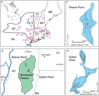
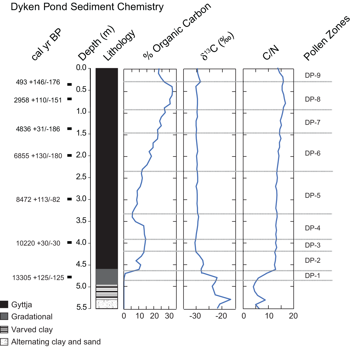
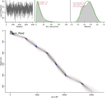
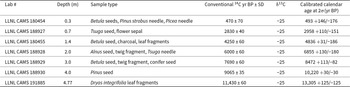
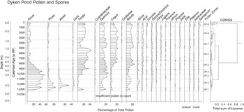
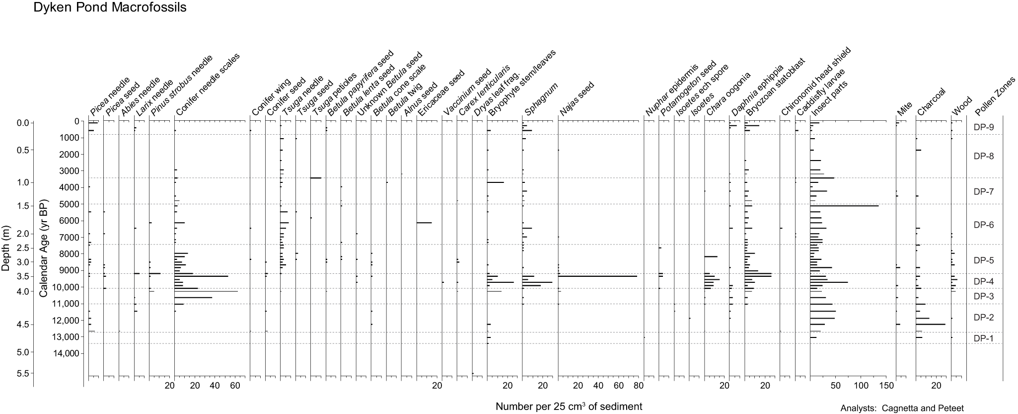
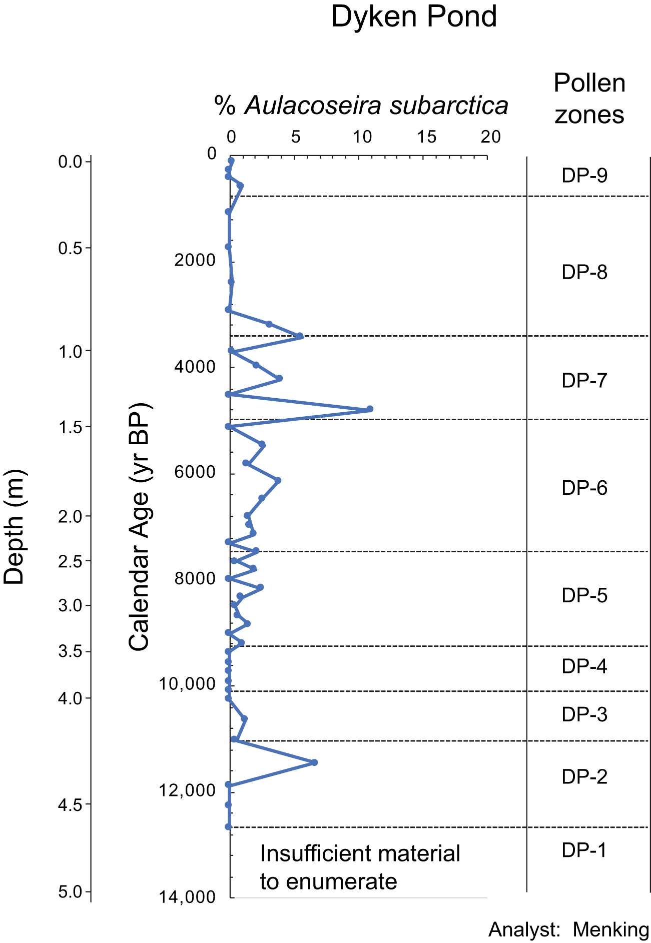
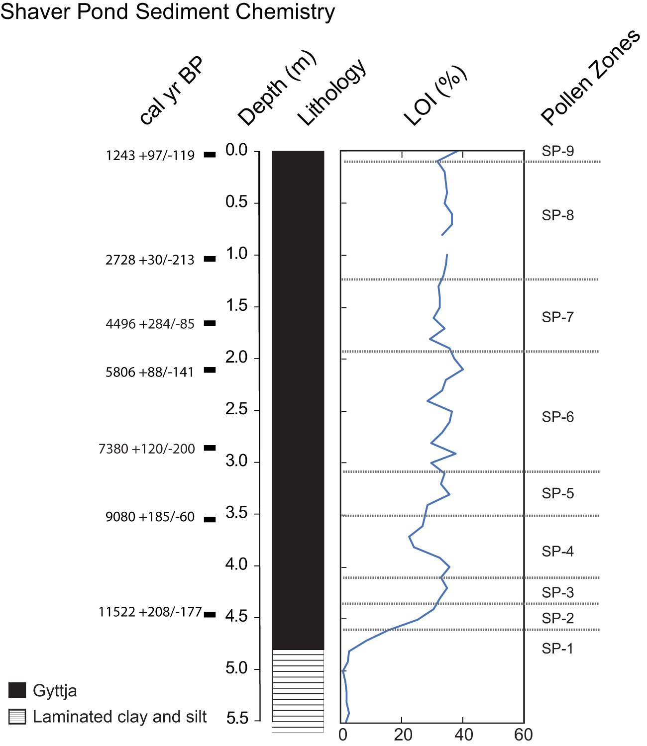
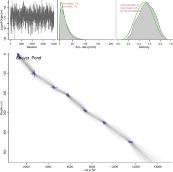
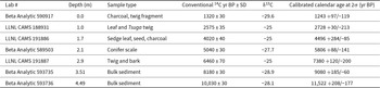
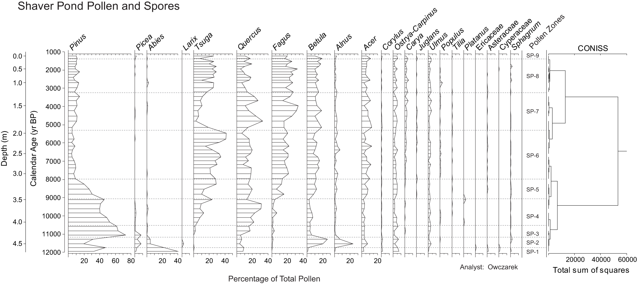
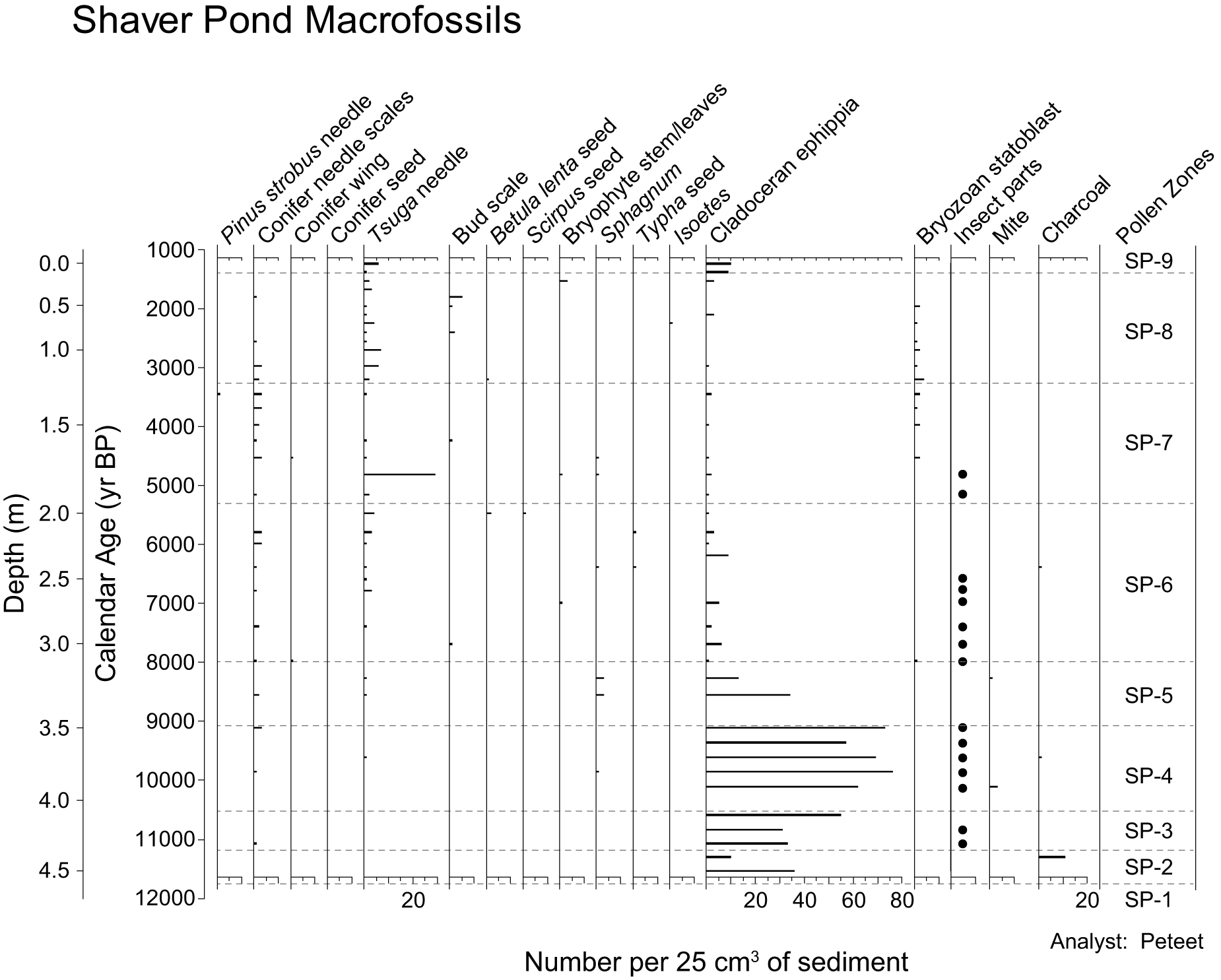
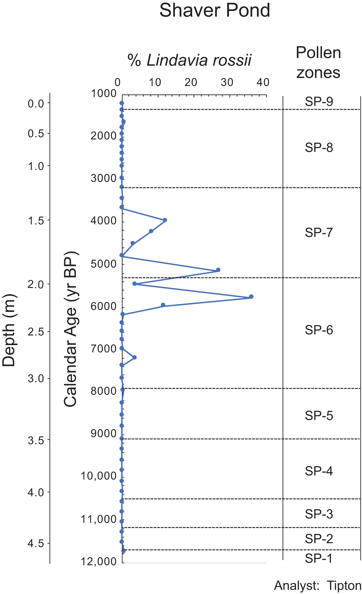
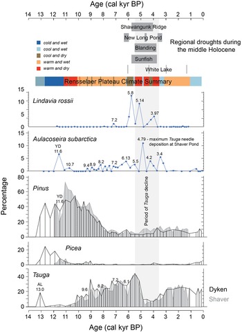


 Open access

