





1. Introduction
1.1. Passive modification of momentum and heat transfer using surfaces
Passive means of affecting turbulent flows for flow control purposes is an area of intense research. Different surfaces such as riblets, roughness and porous walls can alter the dynamics of flow turbulence (Gómez-de Segura & García-Mayoral Reference Gómez-de Segura and García-Mayoral2019; Chung et al. Reference Chung, Hutchins, Schultz and Flack2021; Endrikat et al. Reference Endrikat, Modesti, García-Mayoral, Hutchins and Chung2021; Habibi Khorasani, Luhar & Bagheri Reference Habibi Khorasani, Luhar and Bagheri2024; Hao & García-Mayoral Reference Hao and García-Mayoral2025). This, in turn, has motivated studies on the difference between turbulent heat transfer over such surfaces and smooth walls (Dipprey & Sabersky Reference Dipprey and Sabersky1963; Webb, Eckert & Goldstein Reference Webb, Eckert and Goldstein1971; Han & Zhang Reference Han and Zhang1992; García et al. Reference García, Solano, Vicente and Viedma2012). Leonardi et al. (Reference Leonardi, Orlandi, Djenidi and Antonia2015) investigated turbulent heat transfer over surfaces with transverse bars using direct numerical simulations (DNSs). They showed that the heat flux over the rough surfaces was higher than a smooth wall, although it was always accompanied by an even greater increase in drag. This difference in turbulent momentum and heat transfer was due to the flow separation occurring near the roughness elements, leading to increased contributions from pressure drag, which has no heat-transfer analogue (Owen & Thomson Reference Owen and Thomson1963).
Dissimilarity in the transport mechanisms of heat and momentum transfer means a breakdown of the Reynolds analogy (Von Kármán Reference Von Kármán1939), which can be assessed by the ratio $2St/C_{\kern-1pt f}$
, where
$2St/C_{\kern-1pt f}$
, where $ \textit{St}$
is the Stanton number and
$ \textit{St}$
is the Stanton number and $C_{\kern-1pt f}$
the skin-friction coefficient. Deviations from unity represent a breakdown in the Reynolds analogy, which can be favourable (greater rate of increase in
$C_{\kern-1pt f}$
the skin-friction coefficient. Deviations from unity represent a breakdown in the Reynolds analogy, which can be favourable (greater rate of increase in $ \textit{St}$
relative to the rate of increase in
$ \textit{St}$
relative to the rate of increase in $C_{\kern-1pt f}$
) or unfavourable (lower rate of increase in
$C_{\kern-1pt f}$
) or unfavourable (lower rate of increase in $ \textit{St}$
relative to the rate of increase in
$ \textit{St}$
relative to the rate of increase in $C_{\kern-1pt f}$
). For the bar-type roughness investigated by Leonardi et al. (Reference Leonardi, Orlandi, Djenidi and Antonia2015), the breakdown is unfavourable.
$C_{\kern-1pt f}$
). For the bar-type roughness investigated by Leonardi et al. (Reference Leonardi, Orlandi, Djenidi and Antonia2015), the breakdown is unfavourable.
Further investigations of rough-wall turbulent heat transfer were carried out by Peeters & Sandham (Reference Peeters and Sandham2019), who extended the conclusions of Leonardi et al. (Reference Leonardi, Orlandi, Djenidi and Antonia2015) to irregularly rough surfaces. Their results indicated that heat transfer does not increase indefinitely as the size of the viscous-scaled roughness elements increases. This observation was also made by MacDonald, Hutchins & Chung (Reference MacDonald, Hutchins and Chung2019), who conducted minimal-channel DNSs of turbulent heat transfer over walls with sinusoidal roughness of different heights. They observed that, for a given physical roughness size, $ \textit{St}$
achieves a maximum in the transitionally rough regime and subsequently decays monotonically in the form-drag-dominated fully rough regime.
$ \textit{St}$
achieves a maximum in the transitionally rough regime and subsequently decays monotonically in the form-drag-dominated fully rough regime.
Rouhi et al. (Reference Rouhi, Endrikat, Modesti, Sandberg, Oda, Tanimoto, Hutchins and Chung2022) gathered the heat-transfer efficiencies reported throughout the literature for both active and passive methods of affecting heat transfer (see figure 1 of their manuscript). Active methods such as impingement jets and wall blowing/suction demonstrated the greatest favourable performance. Rough surfaces, i.e. passive methods, consistently demonstrate unfavourable performance. Rouhi et al. (Reference Rouhi, Endrikat, Modesti, Sandberg, Oda, Tanimoto, Hutchins and Chung2022) also studied turbulent heat transfer over riblets. Most of the investigated riblets led to an unfavourable breakdown of the Reynolds analogy, with only certain triangular-shaped riblets achieving a locally favourable breakdown.
Much less is known about heat transfer over porous walls. Motoki et al. (Reference Motoki, Tsugawa, Shimizu and Kawahara2022) carried out DNSs of turbulent channel flow with heat transfer over a permeable wall. At higher permeability, a Kelvin–Helmholtz instability was triggered, significantly enhancing both heat transfer and friction drag. This resulted in an ultimate regime in which the Stanton number and skin-friction coefficient became independent of the Reynolds number. However, the permeable wall was modelled using boundary conditions where the wall-normal velocity was proportional to the local pressure fluctuation. Kuwata, Tsuda & Suga (Reference Kuwata, Tsuda and Suga2020), using the lattice Boltzmann method, conducted DNSs of conjugate heat transfer in a turbulent duct flow that was partially filled with a porous medium consisting of square bars. They found the dispersive and turbulent heat fluxes inside the porous wall to be significant. However, they considered only one porous-wall configuration, consequently, it is not well understood how the heat transfer changes with permeability. The purpose of this study is therefore to investigate porous-wall turbulent heat transfer using DNSs that also take into account the heat transfer in the solid phase. The objective is to analyse the effect of different porous walls on heat transfer and flow turbulence. A brief overview of porous-wall turbulence is provided next.
1.2. Porous-wall turbulence
In their investigation of porous-wall turbulence, Gómez-de Segura & García-Mayoral (Reference Gómez-de Segura and García-Mayoral2019) used analytical solutions derived from Brinkman’s equation (Brinkman Reference Brinkman1949), $\boldsymbol{\nabla }{p}=-\,\nu \,{{\unicode{x1D646}}}^{-1}\,\boldsymbol{u}\,+\,\tilde {\nu }\,{\nabla} ^2{\boldsymbol{u}}$
, where
$\boldsymbol{\nabla }{p}=-\,\nu \,{{\unicode{x1D646}}}^{-1}\,\boldsymbol{u}\,+\,\tilde {\nu }\,{\nabla} ^2{\boldsymbol{u}}$
, where $\boldsymbol{u}$
and
$\boldsymbol{u}$
and $p$
are the volume averaged velocity and pressure, respectively, and
$p$
are the volume averaged velocity and pressure, respectively, and $\nu$
and
$\nu$
and $\tilde {\nu }$
are the molecular and the effective macroscopic viscosity, respectively, as boundary conditions to introduce the effect of anisotropic porous walls on a turbulent channel flow. Assuming a permeability tensor,
$\tilde {\nu }$
are the molecular and the effective macroscopic viscosity, respectively, as boundary conditions to introduce the effect of anisotropic porous walls on a turbulent channel flow. Assuming a permeability tensor, $\unicode{x1D646}$
, with only the principal components,
$\unicode{x1D646}$
, with only the principal components, $K_x$
,
$K_x$
, $K_y$
and
$K_y$
and $K_z$
being non-zero (zero off-diagonal components), and streamwise-preferential configurations (
$K_z$
being non-zero (zero off-diagonal components), and streamwise-preferential configurations ( ${K_x}\hspace {-1pt}\gt \hspace {-1pt}{K_y}$
), they showed that turbulence remains smooth-wall-like for small values of the viscous-scaled effective wall-normal permeability (
${K_x}\hspace {-1pt}\gt \hspace {-1pt}{K_y}$
), they showed that turbulence remains smooth-wall-like for small values of the viscous-scaled effective wall-normal permeability ( $\sqrt {K_y^+}\hspace {-1pt}\lt \hspace {-1pt}0.6$
). Beyond this regime, instabilities are triggered, giving rise to spanwise rollers and the flow transitioning to the so-called Kelvin–Helmholtz-like regime, hereafter called the K–H-like regime. The existence of these spanwise rollers had earlier been shown by Jiménez et al. (Reference Jiménez, Uhlmann, Pinelli and Kawahara2001). Using linear stability analysis, they attributed the rollers to shear waves and K–H instabilities occurring at small/moderate to high permeability, respectively. This distinction between high- and low-permeability flow characteristics was also made by Manes, Poggi & Ridolfi (Reference Manes, Poggi and Ridolfi2011), who experimentally studied turbulent boundary layers over isotropic porous foams. They observed that only for the foam with the largest permeability (
$\sqrt {K_y^+}\hspace {-1pt}\lt \hspace {-1pt}0.6$
). Beyond this regime, instabilities are triggered, giving rise to spanwise rollers and the flow transitioning to the so-called Kelvin–Helmholtz-like regime, hereafter called the K–H-like regime. The existence of these spanwise rollers had earlier been shown by Jiménez et al. (Reference Jiménez, Uhlmann, Pinelli and Kawahara2001). Using linear stability analysis, they attributed the rollers to shear waves and K–H instabilities occurring at small/moderate to high permeability, respectively. This distinction between high- and low-permeability flow characteristics was also made by Manes, Poggi & Ridolfi (Reference Manes, Poggi and Ridolfi2011), who experimentally studied turbulent boundary layers over isotropic porous foams. They observed that only for the foam with the largest permeability ( $\sqrt {K^+}\hspace {-3pt}=\hspace {-3pt}17.2$
) did the flow exhibit the frequency associated with the K–H instability. Spanwise rollers have also been observed in riblet flows. Riblet-resolving linear stability analysis indicates that these rollers are not the most amplified K–H modes, but rather marginal modes with a streamwise wavelength of
$\sqrt {K^+}\hspace {-3pt}=\hspace {-3pt}17.2$
) did the flow exhibit the frequency associated with the K–H instability. Spanwise rollers have also been observed in riblet flows. Riblet-resolving linear stability analysis indicates that these rollers are not the most amplified K–H modes, but rather marginal modes with a streamwise wavelength of $\lambda ^+_x \approx 150$
in wall units (Camobreco et al. Reference Camobreco, Endrikat, García-Mayoral, Luhar and Chung2025). Similar wavelengths, significantly longer than the K–H instability wavelength, are observed in some flows over porous walls, suggesting that these rollers are likewise marginal modes. Although the spanwise rollers observed over low to intermediately permeable walls are not caused by a K–H instability, this flow regime is commonly called the K–H-like regime since the rollers are similar.
$\lambda ^+_x \approx 150$
in wall units (Camobreco et al. Reference Camobreco, Endrikat, García-Mayoral, Luhar and Chung2025). Similar wavelengths, significantly longer than the K–H instability wavelength, are observed in some flows over porous walls, suggesting that these rollers are likewise marginal modes. Although the spanwise rollers observed over low to intermediately permeable walls are not caused by a K–H instability, this flow regime is commonly called the K–H-like regime since the rollers are similar.
In a preceding study, Habibi Khorasani et al. (Reference Habibi Khorasani, Luhar and Bagheri2024) conducted DNSs of turbulent open-channel flows over porous lattices with low to intermediate permeabilities. The low-permeability cases retained the near-wall flow characteristics of smooth-wall turbulence while the intermediate-permeability cases fell into the K–H-like regime. The approximate permeability threshold across which this regime change occurred was also in reasonable agreement with the linear stability predictions of Sharma, Gomez-de Segura & García-Mayoral (Reference Sharma, Gomez-de Segura and García-Mayoral2017), Gómez-de Segura et al. (Reference Gómez-de Segura, Sharma and García-Mayoral2018) using their Brinkman-derived permeable-wall boundary conditions.
Illustration of how the texture-coherent flow scales are related to the physical pore dimensions: the region of the porous wall magnified in (a) has its streamwise and spanwise pitches, $s_x^+$
and
$s_x^+$
and $s_z^+$
, marked using the — and
$s_z^+$
, marked using the — and $--$
lines, respectively. The wall-normal pre-multiplied spectral energy
$--$
lines, respectively. The wall-normal pre-multiplied spectral energy $k^+_x k^+_z E^+_{vv}$
at the surface of the porous wall in case
$k^+_x k^+_z E^+_{vv}$
at the surface of the porous wall in case $ \textit{KP1}$
(parameters are given in § 2) is shown in (b), where the area enclosed by the dark-red line represents the ambient turbulence scales. The contours indicated by the — and
$ \textit{KP1}$
(parameters are given in § 2) is shown in (b), where the area enclosed by the dark-red line represents the ambient turbulence scales. The contours indicated by the — and $--$
lines in (b) are the principal energetic scales of the texture-coherent flow component that occur at streamwise and spanwise wavelengths
$--$
lines in (b) are the principal energetic scales of the texture-coherent flow component that occur at streamwise and spanwise wavelengths $\lambda^+_x$
and
$\lambda^+_x$
and $\lambda^+_z$
equal to the porous-wall pitches. The similar-looking but less intense contours at lower wavelengths are the harmonics of the texture-coherent flow.
$\lambda^+_z$
equal to the porous-wall pitches. The similar-looking but less intense contours at lower wavelengths are the harmonics of the texture-coherent flow.

Figure 1. Long description
The image consists of two parts. Part (a) shows a magnified region of a porous wall with streamwise and spanwise pitches marked by dashed lines. Part (b) displays a graph of the wall-normal pre-multiplied spectral energy at the surface of the porous wall. The graph includes contours representing the principal energetic scales of the texture-coherent flow component, which occur at wavelengths equal to the porous-wall pitches. The area enclosed by a dark-red line represents the ambient turbulence scales. The similar-looking but less intense contours at lower wavelengths are the harmonics of the texture-coherent flow.
Aside from the permeability-triggered flow regime change, there is also the flow component induced by the presence of the porous wall. Any solid structure introduces spatial inhomogeneities into the flow field since the flow is forced to navigate around the solid obstructions. The resulting flow component has scales which conform to the spatial wavelengths of the porous wall. This flow component is commonly referred to as the texture-coherent or grain-coherent flow (Fairhall, Abderrahaman-Elena & García-Mayoral Reference Fairhall, Abderrahaman-Elena and García-Mayoral2019; Hao & García-Mayoral Reference Hao and García-Mayoral2025). Its presence is demonstrated in figure 1, which shows the pre-multiplied spectral energy of the wall-normal velocity, $k_x^+k_z^+E_{vv}^+$
, (figure 1
b) for the turbulent flow over the depicted porous wall (figure 1
a). The energy spectrum reveals that, in addition to the turbulent scales of the flow (the area enclosed by the red lines), energetic scales exist at wavelengths equal to the wall-parallel pore spacings
$k_x^+k_z^+E_{vv}^+$
, (figure 1
b) for the turbulent flow over the depicted porous wall (figure 1
a). The energy spectrum reveals that, in addition to the turbulent scales of the flow (the area enclosed by the red lines), energetic scales exist at wavelengths equal to the wall-parallel pore spacings $s_x^+$
and
$s_x^+$
and $s_z^+$
, which are the signature of the texture-coherent flow. The texture-coherent flow undergoes modulation by the surrounding turbulence (Abderrahaman-Elena, Fairhall & García-Mayoral Reference Abderrahaman-Elena, Fairhall and García-Mayoral2019) and the two can also directly interact with one another when their scales overlap. Such interactions make additional nonlinear contributions to the near-wall dynamics.
$s_z^+$
, which are the signature of the texture-coherent flow. The texture-coherent flow undergoes modulation by the surrounding turbulence (Abderrahaman-Elena, Fairhall & García-Mayoral Reference Abderrahaman-Elena, Fairhall and García-Mayoral2019) and the two can also directly interact with one another when their scales overlap. Such interactions make additional nonlinear contributions to the near-wall dynamics.
1.3. Purpose of this study
In this study, turbulent heat transfer over conductive porous lattices comprising cuboid pores covering a range of permeabilities, from small ( $\sqrt {K^+}\approx 1$
) to large (
$\sqrt {K^+}\approx 1$
) to large ( $\sqrt {K^+}\approx 19$
), are numerically investigated. These porous walls span the range of smooth-wall-like to K–H-like flow regimes, and also include configurations with scale overlap between the ambient turbulence and texture-coherent flow. This way, we can examine how heat transfer evolves over porous walls as we increase the permeability and pass through different regimes of porous-wall turbulence. It also allows for comparisons with heat transfer over rough walls in the transitional and fully rough regimes. Additionally, inclusion of conjugate heat transfer permits us to examine whether increasing permeability has a beneficial or detrimental effect on heat transfer. Heat-transfer efficiency is assessed using the Reynolds analogy, following Bunker (Reference Bunker2013) and Rouhi et al. (Reference Rouhi, Endrikat, Modesti, Sandberg, Oda, Tanimoto, Hutchins and Chung2022). The dissimilarity in momentum and heat transfer (Reynolds analogy breakdown) over the porous walls is further studied in terms of near-wall flow events that contribute to the turbulent transport of heat and momentum.
$\sqrt {K^+}\approx 19$
), are numerically investigated. These porous walls span the range of smooth-wall-like to K–H-like flow regimes, and also include configurations with scale overlap between the ambient turbulence and texture-coherent flow. This way, we can examine how heat transfer evolves over porous walls as we increase the permeability and pass through different regimes of porous-wall turbulence. It also allows for comparisons with heat transfer over rough walls in the transitional and fully rough regimes. Additionally, inclusion of conjugate heat transfer permits us to examine whether increasing permeability has a beneficial or detrimental effect on heat transfer. Heat-transfer efficiency is assessed using the Reynolds analogy, following Bunker (Reference Bunker2013) and Rouhi et al. (Reference Rouhi, Endrikat, Modesti, Sandberg, Oda, Tanimoto, Hutchins and Chung2022). The dissimilarity in momentum and heat transfer (Reynolds analogy breakdown) over the porous walls is further studied in terms of near-wall flow events that contribute to the turbulent transport of heat and momentum.
2. Direct numerical simulation set-up
The numerical set-up used here is similar to that of Habibi Khorasani et al. (Reference Habibi Khorasani, Luhar and Bagheri2024) and the interested reader can refer to that work for details. Only the most pertinent aspects as well as any differences are described in this section.
Sketch of the computational domain, similar to that of Habibi Khorasani et al. (Reference Habibi Khorasani, Luhar and Bagheri2024).

Figure 2. Long description
The diagram illustrates a rectangular computational domain with labeled dimensions. The flow direction is indicated by an arrow pointing to the right. The domain has a height of delta and a length of Lx. The width of the domain is divided into two sections: Lz on the right and an unspecified length on the left. The top and bottom boundaries are marked as free-slip. The vertical axis is labeled y, with T at y equals delta at the top and T at y equals negative h at the bottom. The horizontal axis is labeled x on the left and z on the right.
Direct numerical simulations of open-channel flow were conducted in the numerical domain depicted in figure 2. The dimensions of the domain are $(L_x,L_y,L_z)=(2\pi \delta ,\delta + h,\pi \delta )$
, where
$(L_x,L_y,L_z)=(2\pi \delta ,\delta + h,\pi \delta )$
, where $x, y ,z$
refer to the streamwise, wall-normal and spanwise directions,
$x, y ,z$
refer to the streamwise, wall-normal and spanwise directions, $\delta$
is the channel height and
$\delta$
is the channel height and $h=0.3\delta$
the porous-wall thickness. The flow is governed by the incompressible Navier–Stokes equations
$h=0.3\delta$
the porous-wall thickness. The flow is governed by the incompressible Navier–Stokes equations
 \begin{align} \boldsymbol{\nabla }\boldsymbol{\cdot }{\boldsymbol{u}} = 0, \\[-28pt] \nonumber \end{align}
 \begin{align} \cfrac {\partial \boldsymbol{u}}{ \partial t} + \boldsymbol{u}\boldsymbol{\cdot }\boldsymbol{\nabla }{\boldsymbol{u}} = -\cfrac {1}{\rho }\boldsymbol{\nabla }{p} + \nu {{\nabla} }^2{\boldsymbol{u}}+\varPi {\boldsymbol{e}_x}, \\[0pt] \nonumber \end{align}
where $t$
is time,
$t$
is time, $\boldsymbol{u}(\boldsymbol{x}, t)$
is the velocity vector with
$\boldsymbol{u}(\boldsymbol{x}, t)$
is the velocity vector with $(u,v,w)$
the streamwise, wall-normal and spanwise components, respectively,
$(u,v,w)$
the streamwise, wall-normal and spanwise components, respectively, $p(\boldsymbol{x}, t)$
is the pressure,
$p(\boldsymbol{x}, t)$
is the pressure, $\rho$
is the density,
$\rho$
is the density, $\nu$
is the kinematic viscosity,
$\nu$
is the kinematic viscosity, $\boldsymbol{e}_x$
is a unit vector in the streamwise direction and
$\boldsymbol{e}_x$
is a unit vector in the streamwise direction and $\varPi$
is the spatially uniform but temporally varying forcing term, adjusted such that a constant flow rate is maintained in the channel region. The domain is periodic along the
$\varPi$
is the spatially uniform but temporally varying forcing term, adjusted such that a constant flow rate is maintained in the channel region. The domain is periodic along the $x$
and
$x$
and $z$
directions. No-slip and impermeability conditions are imposed at
$z$
directions. No-slip and impermeability conditions are imposed at $y=-h$
while at
$y=-h$
while at $y=\delta$
free-slip and impermeability conditions are imposed. The surface of the porous wall is at
$y=\delta$
free-slip and impermeability conditions are imposed. The surface of the porous wall is at $y=0$
. Heat transfer is incorporated by solving a convection–diffusion equation for a scalar temperature field
$y=0$
. Heat transfer is incorporated by solving a convection–diffusion equation for a scalar temperature field
 \begin{align} \cfrac {\partial T}{\partial t} + (\boldsymbol{u}\boldsymbol{\cdot }\boldsymbol{\nabla }){T} = \alpha {{\nabla} }^2{T}, \end{align}
where $T$
,
$T$
, $\alpha ={\kappa }/(\rho c_p)$
,
$\alpha ={\kappa }/(\rho c_p)$
, $c_p$
and
$c_p$
and $\kappa$
are the temperature, thermal diffusivity, specific heat capacity and thermal conductivity, respectively. Fixed-temperature conditions
$\kappa$
are the temperature, thermal diffusivity, specific heat capacity and thermal conductivity, respectively. Fixed-temperature conditions $T\rvert _{y=-h}$
and
$T\rvert _{y=-h}$
and $T\rvert _{y=\delta }$
are imposed at the bottom and top domain boundaries, respectively, so that heat is transferred from the bottom of the porous wall to the top of the channel region. The temperature is a passive scalar since buoyancy effects are neglected in the present study.
$T\rvert _{y=\delta }$
are imposed at the bottom and top domain boundaries, respectively, so that heat is transferred from the bottom of the porous wall to the top of the channel region. The temperature is a passive scalar since buoyancy effects are neglected in the present study.
Equations (2.1)–(2.2) are solved using the open-source solver CaNS (Costa Reference Costa2018; Costa et al. Reference Costa, Phillips, Brandt and Fatica2021; Diez Sanhueza et al. Reference Diez Sanhueza, Peeters and Costa2025), which discretises them using second-order central finite differences on structured Cartesian grids using a staggered arrangement. The grids used are uniform along $x$
and
$x$
and $z$
. In the
$z$
. In the $y$
-direction, the grid is stretched in the channel region of the domain using a hyperbolic tangent function and uniform across the porous region.
$y$
-direction, the grid is stretched in the channel region of the domain using a hyperbolic tangent function and uniform across the porous region.
The porous substrate has essentially the same structure as in the DNSs by Habibi Khorasani et al. (Reference Habibi Khorasani, Luhar and Bagheri2024) and consists of a matrix of interconnected square bars with a cross-section of $d\times d$
aligned with the
$d\times d$
aligned with the $x$
,
$x$
, $y$
and
$y$
and $z$
directions. The bar spacings (pitches)
$z$
directions. The bar spacings (pitches) $s_x$
,
$s_x$
, $s_y$
and
$s_y$
and $s_z$
in the streamwise, wall-normal and spanwise directions, respectively (see figure 1), are systematically varied, while
$s_z$
in the streamwise, wall-normal and spanwise directions, respectively (see figure 1), are systematically varied, while $d=0.039\delta$
is kept constant in the DNSs, resulting in a range of porosities and anisotropic permeabilities. The purpose of these variations is to obtain a meaningful flow transition with increasing permeability; from smooth-wall-like behaviour to flow states featuring spanwise rollers and strongly enhanced turbulence.
$d=0.039\delta$
is kept constant in the DNSs, resulting in a range of porosities and anisotropic permeabilities. The purpose of these variations is to obtain a meaningful flow transition with increasing permeability; from smooth-wall-like behaviour to flow states featuring spanwise rollers and strongly enhanced turbulence.
Similar porous structures composed of interconnected square bars have been used in numerical (Hao & García-Mayoral Reference Hao and García-Mayoral2025) and experimental studies (Suga, Okazaki & Kuwata Reference Suga, Okazaki and Kuwata2020; Vijay & Luhar Reference Vijay and Luhar2024), as they are straightforward to characterise and relatively easy to fabricate (e.g. via additive manufacturing). The porous interface in the present study is chosen to be flat to isolate the effect of the permeability on the flow and heat transfer. Protruding elements at the interface can act as roughness and increase drag (Suga et al. Reference Suga, Okazaki and Kuwata2020; Hao & García-Mayoral Reference Hao and García-Mayoral2025). Previous work indicates that when the porous structure (i.e. bar spacing) is sufficiently fine ( $\lesssim 50$
viscous wall units) the macroscopic properties, i.e. permeability, have a much larger impact on the mean flow, Reynolds stresses and spectra than the detailed structure of the porous substrate (Hao & García-Mayoral Reference Hao and García-Mayoral2025). This observation suggests that the results of our study are also relevant for turbulent flows and heat transfer over other porous substrates with different structures but similar permeabilities. Only in the cases with the largest bar spacings can the texture-coherent flow directly interact with the overlying turbulence. In such cases, the specific structure of the porous substrate has a larger effect on the flow statistics and heat transfer.
$\lesssim 50$
viscous wall units) the macroscopic properties, i.e. permeability, have a much larger impact on the mean flow, Reynolds stresses and spectra than the detailed structure of the porous substrate (Hao & García-Mayoral Reference Hao and García-Mayoral2025). This observation suggests that the results of our study are also relevant for turbulent flows and heat transfer over other porous substrates with different structures but similar permeabilities. Only in the cases with the largest bar spacings can the texture-coherent flow directly interact with the overlying turbulence. In such cases, the specific structure of the porous substrate has a larger effect on the flow statistics and heat transfer.
The porous walls are numerically represented using the immersed-boundary method of Breugem & Boersma (Reference Breugem and Boersma2005) and Paravento, Pourquie & Boersma (Reference Paravento, Pourquie and Boersma2008) for grid-conforming Cartesian geometries. It involves modifying the discretised advective and diffusive fluxes of cells identified as solids such that the no-slip condition becomes exactly imposed, giving second-order spatial accuracy. The grid resolution used is the same as that in Habibi Khorasani et al. (Reference Habibi Khorasani, Luhar and Bagheri2024), with the number of grid points being $(N_x,N_y,N_z)=(1620, 324, 810)$
. The square bars are resolved with
$(N_x,N_y,N_z)=(1620, 324, 810)$
. The square bars are resolved with $10$
grid points in the streamwise and spanwise directions, and
$10$
grid points in the streamwise and spanwise directions, and $25$
grid points in the wall-normal direction.
$25$
grid points in the wall-normal direction.
CaNS integrates the equations in time using a fractional-step pressure-correction algorithm. To remove the diffusive constraint on the time step used for temporal integration, the diffusive terms can be treated implicitly by solving a Helmholtz equation for each of the velocity components. However, to benefit from this in our conjugate heat-transfer simulations that have a spatially varying thermal diffusivity in the porous wall, we use the method of Dodd & Ferrante (Reference Dodd and Ferrante2014) to split the diffusive term into a variable term and a constant term, with the former treated implicitly and the latter explicitly. This prevents the greater thermal diffusivity in the solid phase from imposing a strict restriction on the time step.
The relevant non-dimensional quantities for characterising the flow are the bulk Reynolds number, $ \textit{Re}_b = U_b\delta /\nu$
, and the Prandtl number,
$ \textit{Re}_b = U_b\delta /\nu$
, and the Prandtl number, $ \textit{Pr} = \nu /\alpha$
. The simulations were conducted at a targeted
$ \textit{Pr} = \nu /\alpha$
. The simulations were conducted at a targeted $ \textit{Re}_{\tau } = u_{\tau }\delta /\nu = 360$
, defined based on the channel region of the domain (
$ \textit{Re}_{\tau } = u_{\tau }\delta /\nu = 360$
, defined based on the channel region of the domain ( $0 \leqslant y \leqslant \delta$
) and achieved by adjusting
$0 \leqslant y \leqslant \delta$
) and achieved by adjusting $ \textit{Re}_b$
. Here,
$ \textit{Re}_b$
. Here, $u_{\tau }=\sqrt {{\tau _{w}}/{\rho }}$
is the friction velocity and
$u_{\tau }=\sqrt {{\tau _{w}}/{\rho }}$
is the friction velocity and $\tau _{w}$
is the mean shear stress at
$\tau _{w}$
is the mean shear stress at $y=0$
. At this
$y=0$
. At this $ \textit{Re}_\tau$
,
$ \textit{Re}_\tau$
, $h^+ \approx 100$
and therefore the porous substrate can be considered deep and no substantial change in the overlying turbulent flow is expected when
$h^+ \approx 100$
and therefore the porous substrate can be considered deep and no substantial change in the overlying turbulent flow is expected when $h$
is further increased (Hao & García-Mayoral Reference Hao and García-Mayoral2025). For the thermal property of the working fluid,
$h$
is further increased (Hao & García-Mayoral Reference Hao and García-Mayoral2025). For the thermal property of the working fluid, $ \textit{Pr} = 0.71$
was used, which corresponds to air. A thermal diffusivity of
$ \textit{Pr} = 0.71$
was used, which corresponds to air. A thermal diffusivity of $\alpha _s = 4.4\alpha _f$
was set for the solid phase to make it analogous to aluminium.
$\alpha _s = 4.4\alpha _f$
was set for the solid phase to make it analogous to aluminium.
Direct numerical simulations of turbulent channel flow over porous walls by Hao & García-Mayoral (Reference Hao and García-Mayoral2025) showed that the mean velocity, near-wall fluctuation profiles and spectra agree well at $ \textit{Re}_\tau = 180$
, 360 and 550 when the porous substrate dimensions (and thus the permeability) are matched in wall units. Hao & García-Mayoral (Reference Hao and García-Mayoral2025) also considered four porous-wall cases with a flat interface, as in the present study and Habibi Khorasani et al. (Reference Habibi Khorasani, Luhar and Bagheri2024), and found that the mean-velocity profile shift in their DNS at
$ \textit{Re}_\tau = 180$
, 360 and 550 when the porous substrate dimensions (and thus the permeability) are matched in wall units. Hao & García-Mayoral (Reference Hao and García-Mayoral2025) also considered four porous-wall cases with a flat interface, as in the present study and Habibi Khorasani et al. (Reference Habibi Khorasani, Luhar and Bagheri2024), and found that the mean-velocity profile shift in their DNS at $ \textit{Re}_\tau = 180$
and ours at
$ \textit{Re}_\tau = 180$
and ours at $ \textit{Re}_\tau = 360$
follows the same trend with permeability. These observations suggest that the findings in the present study extend to other Reynolds numbers.
$ \textit{Re}_\tau = 360$
follows the same trend with permeability. These observations suggest that the findings in the present study extend to other Reynolds numbers.
Variables $\phi$
are decomposed using the Reynolds decomposition
$\phi$
are decomposed using the Reynolds decomposition
 \begin{gather} {\phi }(x,y,z,t) = {\varPhi }(y) + \phi ^{\prime }(x,y,z,t), \end{gather}
where $\phi$
is the instantaneous value ,
$\phi$
is the instantaneous value , $\varPhi$
is the time- and plane-averaged mean value and
$\varPhi$
is the time- and plane-averaged mean value and $\phi ^{\prime }$
is the full time-and-space varying fluctuation. The latter can be further decomposed into (Reynolds & Hussain Reference Reynolds and Hussain1972)
$\phi ^{\prime }$
is the full time-and-space varying fluctuation. The latter can be further decomposed into (Reynolds & Hussain Reference Reynolds and Hussain1972)
 \begin{gather} \phi ^{\prime }(x,y,z,t) = \tilde {\phi }(x,y,z) + \phi ^{\prime \prime }(x,y,z,t), \end{gather}
where $\tilde {\phi }(x,y,z)$
is the time-invariant but spatially varying dispersive component induced by the porous wall and
$\tilde {\phi }(x,y,z)$
is the time-invariant but spatially varying dispersive component induced by the porous wall and $\phi ^{\prime \prime }(x,y,z,t)$
the remaining time-and-space varying fluctuation due to turbulence.
$\phi ^{\prime \prime }(x,y,z,t)$
the remaining time-and-space varying fluctuation due to turbulence.
Plane-averaged flow and temperature statistics are reported as fluid-averaged and solid-averaged quantities over a region $S_i$
$S_i$
 \begin{gather} {\varPhi }_i(y) = \cfrac {1}{A_i}\iint _{S_i}{{\hat {\phi }(x,y,z)}}\,{\rm d}x\,{\rm d}z, \end{gather}
where $A_i$
is the area of that region,
$A_i$
is the area of that region, $\hat {\phi }(x,y,z)$
is the time-averaged value of
$\hat {\phi }(x,y,z)$
is the time-averaged value of $\phi (x,y,z,t)$
and
$\phi (x,y,z,t)$
and $i = f, s$
indicates over which phase the plane averaging has been done (
$i = f, s$
indicates over which phase the plane averaging has been done ( $f$
for fluid and
$f$
for fluid and $s$
for solid). Since the flow velocities are zero in the solid-occupied regions, all velocity-related statistics are fluid-phase averages, and so the subscript
$s$
for solid). Since the flow velocities are zero in the solid-occupied regions, all velocity-related statistics are fluid-phase averages, and so the subscript $f$
is dropped. The temperature field, however, is present throughout both phases. The ‘
$f$
is dropped. The temperature field, however, is present throughout both phases. The ‘ $+$
’ superscript indicates viscous-scaled quantities using
$+$
’ superscript indicates viscous-scaled quantities using $u_{\tau }$
and
$u_{\tau }$
and $\nu$
. The non-dimensional temperature
$\nu$
. The non-dimensional temperature $\theta$
is defined as
$\theta$
is defined as
 \begin{gather} \theta = \cfrac {T-T\rvert _{y=\delta }}{T\rvert _{y=-h} - T\rvert _{y=\delta }}, \end{gather}
so that $\theta = 1$
at
$\theta = 1$
at $y=-h$
and
$y=-h$
and $\theta =0$
at
$\theta =0$
at $y=\delta$
.
$y=\delta$
.
A summary of all DNS cases and their relevant parameters is given in table 1. Here, the porosity $\varphi$
is the volume fraction of the fluid in a representative elementary volume (Habibi Khorasani et al. Reference Habibi Khorasani, Luhar and Bagheri2024). The zero-permeability case,
$\varphi$
is the volume fraction of the fluid in a representative elementary volume (Habibi Khorasani et al. Reference Habibi Khorasani, Luhar and Bagheri2024). The zero-permeability case, $ \textit{ZP}$
, is the baseline smooth-wall case where the wall region is a solid impenetrable block. The smooth-wall-like permeable case,
$ \textit{ZP}$
, is the baseline smooth-wall case where the wall region is a solid impenetrable block. The smooth-wall-like permeable case, $ \textit{SP}$
, has low permeability and retains the smooth-wall-like structure of near-wall turbulence. The transitionally permeable case,
$ \textit{SP}$
, has low permeability and retains the smooth-wall-like structure of near-wall turbulence. The transitionally permeable case, $ \textit{TP}$
, shows signs of departing the smooth-wall-like regime. The K–H permeable cases,
$ \textit{TP}$
, shows signs of departing the smooth-wall-like regime. The K–H permeable cases, $ \textit{KP}\langle \rangle$
, fall into the K–H-like regime of wall turbulence. We use here and hereafter the notation
$ \textit{KP}\langle \rangle$
, fall into the K–H-like regime of wall turbulence. We use here and hereafter the notation $ \textit{KP}\langle \rangle$
to refer collectively to the subcases
$ \textit{KP}\langle \rangle$
to refer collectively to the subcases $ \textit{KP1}$
,
$ \textit{KP1}$
, $ \textit{KP2}$
and
$ \textit{KP2}$
and $ \textit{KP3}$
. The walls of cases
$ \textit{KP3}$
. The walls of cases $ \textit{SP}$
,
$ \textit{SP}$
, $ \textit{TP}$
,
$ \textit{TP}$
, $ \textit{KP3}$
,
$ \textit{KP3}$
, $ \textit{KP2}$
and
$ \textit{KP2}$
and $ \textit{KP1}$
, respectively, correspond to cases
$ \textit{KP1}$
, respectively, correspond to cases $ \textit{LP1}$
,
$ \textit{LP1}$
, $ \textit{MP}$
,
$ \textit{MP}$
, $ \textit{HP3}$
,
$ \textit{HP3}$
, $ \textit{HP2}$
and
$ \textit{HP2}$
and $ \textit{HP1}$
of Habibi Khorasani et al. (Reference Habibi Khorasani, Luhar and Bagheri2024), where it was established to which flow regime each case belonged. Habibi Khorasani et al. (Reference Habibi Khorasani, Luhar and Bagheri2024) also provide schematics and visualisations of some of the considered porous substrates. The off-diagonal permeabilities of the porous structures are zero, while the diagonal permeabilities,
$ \textit{HP1}$
of Habibi Khorasani et al. (Reference Habibi Khorasani, Luhar and Bagheri2024), where it was established to which flow regime each case belonged. Habibi Khorasani et al. (Reference Habibi Khorasani, Luhar and Bagheri2024) also provide schematics and visualisations of some of the considered porous substrates. The off-diagonal permeabilities of the porous structures are zero, while the diagonal permeabilities, $\sqrt {K_{i}^+}$
, were obtained using Darcy’s law,
$\sqrt {K_{i}^+}$
, were obtained using Darcy’s law, $\boldsymbol{\nabla }{p}=-\nu \,{{\unicode{x1D646}}}^{-1}\boldsymbol{\cdot }\boldsymbol{u}$
, by conducting Stokes simulations in representative elementary volumes of each porous wall. The
$\boldsymbol{\nabla }{p}=-\nu \,{{\unicode{x1D646}}}^{-1}\boldsymbol{\cdot }\boldsymbol{u}$
, by conducting Stokes simulations in representative elementary volumes of each porous wall. The $ \textit{KP}\langle \rangle a$
and
$ \textit{KP}\langle \rangle a$
and $ \textit{KP}\langle \rangle b$
cases retain the same wall-normal pitches,
$ \textit{KP}\langle \rangle b$
cases retain the same wall-normal pitches, $s_y$
, as the
$s_y$
, as the $ \textit{KP}\langle \rangle$
case but have successively larger wall-parallel pitches,
$ \textit{KP}\langle \rangle$
case but have successively larger wall-parallel pitches, $s_x$
and
$s_x$
and $s_z$
. The purpose of this successive increase in
$s_z$
. The purpose of this successive increase in $s_x$
and
$s_x$
and $s_z$
, in addition to increasing permeability, was to cause the texture-coherent scales to overlap with those of the ambient turbulence as discussed in § 1.2, and to further enhance the heat transfer.
$s_z$
, in addition to increasing permeability, was to cause the texture-coherent scales to overlap with those of the ambient turbulence as discussed in § 1.2, and to further enhance the heat transfer.
Parameters of the DNS cases. The pore pitch lengths are ${s_{x}}^+$
,
${s_{x}}^+$
, ${s_{y}}^+$
and
${s_{y}}^+$
and ${s_{z}}^+$
, while
${s_{z}}^+$
, while $\sqrt {K_{x}^+}$
,
$\sqrt {K_{x}^+}$
, $\sqrt {K_{y}^+}$
and
$\sqrt {K_{y}^+}$
and $\sqrt {K_{z}^+}$
are the effective permeabilities which are equivalent to the permeability Reynolds number,
$\sqrt {K_{z}^+}$
are the effective permeabilities which are equivalent to the permeability Reynolds number, $ \textit{Re}_{K}$
, used throughout the literature. The ratio of streamwise to wall-normal permeability serves as the measure of a wall’s anisotropy.
$ \textit{Re}_{K}$
, used throughout the literature. The ratio of streamwise to wall-normal permeability serves as the measure of a wall’s anisotropy.

In all cases, $d^+=14$
and the spanwise and streamwise grid spacing is
$d^+=14$
and the spanwise and streamwise grid spacing is $1.4$
wall units, which is sufficient to resolve the turbulence. The wall-normal grid spacing is uniform and
$1.4$
wall units, which is sufficient to resolve the turbulence. The wall-normal grid spacing is uniform and $0.56$
wall units in the porous substrate, whereas it is stretched away from the porous wall. Further details and a resolution assessment for the flow in and over the porous substrate are provided in Habibi Khorasani et al. (Reference Habibi Khorasani, Luhar and Bagheri2024), noting that the present study uses the same resolution. The
$0.56$
wall units in the porous substrate, whereas it is stretched away from the porous wall. Further details and a resolution assessment for the flow in and over the porous substrate are provided in Habibi Khorasani et al. (Reference Habibi Khorasani, Luhar and Bagheri2024), noting that the present study uses the same resolution. The $ \textit{KP}\langle \rangle$
cases use
$ \textit{KP}\langle \rangle$
cases use $15-67$
and
$15-67$
and $10-50$
grid points per gap in the streamwise and spanwise directions, respectively. The grid sensitivity study by Habibi Khorasani et al. (Reference Habibi Khorasani, Luhar and Bagheri2024) shows that 15 and 10 grid points per gap in the streamwise and spanwise directions, respectively, is sufficient to resolve the flow in and over the porous substrate. Kuwata et al. (Reference Kuwata, Tsuda and Suga2020) performed DNSs of conjugate heat transfer in duct flow with a porous wall composed of square bars using the same
$10-50$
grid points per gap in the streamwise and spanwise directions, respectively. The grid sensitivity study by Habibi Khorasani et al. (Reference Habibi Khorasani, Luhar and Bagheri2024) shows that 15 and 10 grid points per gap in the streamwise and spanwise directions, respectively, is sufficient to resolve the flow in and over the porous substrate. Kuwata et al. (Reference Kuwata, Tsuda and Suga2020) performed DNSs of conjugate heat transfer in duct flow with a porous wall composed of square bars using the same $ \textit{Pr}$
and solid to fluid thermal diffusivity ratio as used here. They compared a simulation using a
$ \textit{Pr}$
and solid to fluid thermal diffusivity ratio as used here. They compared a simulation using a $23\times 23$
grid to resolve each bar with a second case with twice the grid spacing and found no significant differences. In our DNSs, the streamwise and spanwise resolutions per bar are comparable to their coarse case, whereas the wall-normal resolution is comparable to their refined case. Our resolution should therefore be adequate to resolve both the flow and heat transfer.
$23\times 23$
grid to resolve each bar with a second case with twice the grid spacing and found no significant differences. In our DNSs, the streamwise and spanwise resolutions per bar are comparable to their coarse case, whereas the wall-normal resolution is comparable to their refined case. Our resolution should therefore be adequate to resolve both the flow and heat transfer.
Time history of (a) the bulk temperature and (b) the total heat flux at the top boundary.

Figure 3. Long description
The image contains two line graphs. The first graph (a) shows the time history of bulk temperature with the y-axis labeled theta ranging from 0.30 to 0.44 and the x-axis labeled t* (U_b/δ) ranging from 600 to 1600. Multiple colored lines represent different data series, each maintaining relatively stable values over time. The second graph (b) illustrates the time history of total heat flux at the top boundary with the y-axis labeled q_total in units of 10−3 and the x-axis labeled t* (U_b/δ) ranging from 600 to 1600. Multiple colored lines represent different data series, showing fluctuations over time. The graphs are used to analyze the effects of different surfaces on turbulent flows and heat transfer.
Each DNS case of table 1 was first run for a time period of $2000 \delta /U_b$
so that the flow and temperature fields reached fully developed, statistically stationary conditions. The DNSs were then continued for an additional time period of
$2000 \delta /U_b$
so that the flow and temperature fields reached fully developed, statistically stationary conditions. The DNSs were then continued for an additional time period of $2000 \delta /U_b$
to collect statistics. Statistical steadiness is evidenced in figure 3, which shows a part of the time history of the bulk temperature and total heat flux.
$2000 \delta /U_b$
to collect statistics. Statistical steadiness is evidenced in figure 3, which shows a part of the time history of the bulk temperature and total heat flux.
3. Results
3.1. Flow differences over the different porous walls
Before analysing the heat transfer, the velocity fields for the cases of table 1 in the channel region ( $y\gt 0$
) are briefly examined to establish their features. Since heat transfer is passive, structural changes in the velocity field will largely determine any differences that emerge in the temperature fields for the different walls.
$y\gt 0$
) are briefly examined to establish their features. Since heat transfer is passive, structural changes in the velocity field will largely determine any differences that emerge in the temperature fields for the different walls.
Profiles of the (a) mean velocity, (b) Reynolds shear stress, (c) root-mean-square velocity fluctuations. The direction of the grey arrow in (a) and (b) indicates increasing wall-normal permeability. In (b); —, total Reynolds stress; $--$
, dispersive Reynolds stress. In (c); —, total streamwise fluctuations;
$--$
, dispersive Reynolds stress. In (c); —, total streamwise fluctuations; $--$
, total spanwise fluctuations;
$--$
, total spanwise fluctuations; $\boldsymbol{\cdot }\!\boldsymbol{\cdot }\!\boldsymbol{\cdot}$
, total wall-normal fluctuations. The open circles,
$\boldsymbol{\cdot }\!\boldsymbol{\cdot }\!\boldsymbol{\cdot}$
, total wall-normal fluctuations. The open circles, $\circ$
, are reference smooth-wall data produced using a pseudo-spectral solver.
$\circ$
, are reference smooth-wall data produced using a pseudo-spectral solver.

Figure 4. Long description
The image contains three line graphs labeled (a), (b), and (c). Graph (a) shows the mean velocity (U+) against the wall-normal coordinate (y+). Graph (b) displays the Reynolds shear stress components (u’v+ and u’v+_d) against y+. Graph (c) illustrates the root-mean-square velocity fluctuations (u’_rms+, v’_rms+, and w’_rms+) against y+. The direction of the grey arrow in (a) and (b) indicates increasing wall-normal permeability. The open circles represent reference smooth-wall data produced using a pseudo-spectral solver. The graphs compare turbulent flow characteristics over different surfaces, including porous walls, and highlight the differences in heat transfer and drag.
Figure 4(a) shows the plane- and time-averaged mean-velocity profiles. It is clear that, as the permeability grows, the mean-velocity deficit relative to the smooth-wall case, $ \textit{ZP}$
, also becomes larger. The mean-velocity profile in the low-permeability case
$ \textit{ZP}$
, also becomes larger. The mean-velocity profile in the low-permeability case $ \textit{SP}$
does not differ much from that in case
$ \textit{SP}$
does not differ much from that in case $ \textit{ZP}$
, but in the high-permeability cases, and especially in
$ \textit{ZP}$
, but in the high-permeability cases, and especially in $ \textit{KP}\langle \rangle b$
, the difference is large. The differences observed in figure 4(a) for the mean velocities are reflected in figure 4(b) for the total Reynolds shear stress profiles,
$ \textit{KP}\langle \rangle b$
, the difference is large. The differences observed in figure 4(a) for the mean velocities are reflected in figure 4(b) for the total Reynolds shear stress profiles, $-\overline {{u^{\prime }}{v^{\prime }}}^+$
. Here and below, an overline denotes time and planar averaging. Obviously, the
$-\overline {{u^{\prime }}{v^{\prime }}}^+$
. Here and below, an overline denotes time and planar averaging. Obviously, the $ \textit{KP}\langle \rangle$
,
$ \textit{KP}\langle \rangle$
, $ \textit{KP}\langle \rangle a$
and
$ \textit{KP}\langle \rangle a$
and $ \textit{KP}\langle \rangle b$
profiles fall into separate groups in the near-wall region. The strength of the Reynolds shear stress progressively grows in this region as the wall becomes more permeable and is more uniform. These higher stress levels at the surface cause the lower mean velocities shown in figure 4(a). The change of
$ \textit{KP}\langle \rangle b$
profiles fall into separate groups in the near-wall region. The strength of the Reynolds shear stress progressively grows in this region as the wall becomes more permeable and is more uniform. These higher stress levels at the surface cause the lower mean velocities shown in figure 4(a). The change of $-\overline {{u^{\prime }}{v^{\prime }}}^+$
profiles indicates structural changes in turbulence. This change can also be inferred from the root-mean-square (r.m.s.) velocity fluctuations in figure 4(c). The near-wall peak of the
$-\overline {{u^{\prime }}{v^{\prime }}}^+$
profiles indicates structural changes in turbulence. This change can also be inferred from the root-mean-square (r.m.s.) velocity fluctuations in figure 4(c). The near-wall peak of the $u$
velocity fluctuations strongly decreases as the wall becomes more permeable. The fluctuations of
$u$
velocity fluctuations strongly decreases as the wall becomes more permeable. The fluctuations of $w$
and
$w$
and $v$
, however, grow more intense, such that the turbulence becomes more isotropic. A higher permeability also allows turbulent motions to penetrate into the wall, leading to a rise in the r.m.s. values for all three velocity components. While not shown here, it can readily be deduced from figures 4(b) and 4(c) that, in the K–H-like
$v$
, however, grow more intense, such that the turbulence becomes more isotropic. A higher permeability also allows turbulent motions to penetrate into the wall, leading to a rise in the r.m.s. values for all three velocity components. While not shown here, it can readily be deduced from figures 4(b) and 4(c) that, in the K–H-like $ \textit{KP}$
cases, the turbulent stresses penetrate into the wall. This penetration is quite deep for the highly permeable
$ \textit{KP}$
cases, the turbulent stresses penetrate into the wall. This penetration is quite deep for the highly permeable $ \textit{KP}\langle \rangle b$
cases, as will become clear later. The mean and fluctuating velocity profiles of case
$ \textit{KP}\langle \rangle b$
cases, as will become clear later. The mean and fluctuating velocity profiles of case $ \textit{ZP}$
in figures 4(a), 4(b) and 4(c) agree well with reference smooth-wall open-channel DNS data at
$ \textit{ZP}$
in figures 4(a), 4(b) and 4(c) agree well with reference smooth-wall open-channel DNS data at $ \textit{Re}_\tau = 360$
obtained with a pseudospectral solver (Chevalier et al. Reference Chevalier, Schlatter, Lundbladh and Henningson2014), as used in e.g. Brethouwer (Reference Brethouwer2017).
$ \textit{Re}_\tau = 360$
obtained with a pseudospectral solver (Chevalier et al. Reference Chevalier, Schlatter, Lundbladh and Henningson2014), as used in e.g. Brethouwer (Reference Brethouwer2017).
Figure 4(b) also shows the planar-averaged dispersive component of the Reynolds shear stress for the highly permeable cases $ \textit{KP1}$
,
$ \textit{KP1}$
, $ \textit{KP}1 a$
,
$ \textit{KP}1 a$
, $ \textit{KP}1 b$
,
$ \textit{KP}1 b$
, $ \textit{KP2}$
,
$ \textit{KP2}$
, $ \textit{KP}2 a$
and
$ \textit{KP}2 a$
and $ \textit{KP}2 b$
. It is evident that, even for the most permeable walls, the dispersive contribution to the total Reynolds shear stress throughout the bulk flow region is negligible. The dispersive shear stress does appear to grow around
$ \textit{KP}2 b$
. It is evident that, even for the most permeable walls, the dispersive contribution to the total Reynolds shear stress throughout the bulk flow region is negligible. The dispersive shear stress does appear to grow around $y+\approx 150$
with growing permeability (and hence stronger K–H-like rollers), and is slightly negative close to the porous wall. This negative shear stress is caused by the K–H-like rollers, which can induce negative shear (Endrikat et al. Reference Endrikat, Modesti, García-Mayoral, Hutchins and Chung2021; Rouhi et al. Reference Rouhi, Endrikat, Modesti, Sandberg, Oda, Tanimoto, Hutchins and Chung2022). Also notable is that, unlike in the case of the canopy structures studied by Chen & García-Mayoral (Reference Chen and García-Mayoral2023), no strong dispersive stresses occur at the surface of the porous wall.
$y+\approx 150$
with growing permeability (and hence stronger K–H-like rollers), and is slightly negative close to the porous wall. This negative shear stress is caused by the K–H-like rollers, which can induce negative shear (Endrikat et al. Reference Endrikat, Modesti, García-Mayoral, Hutchins and Chung2021; Rouhi et al. Reference Rouhi, Endrikat, Modesti, Sandberg, Oda, Tanimoto, Hutchins and Chung2022). Also notable is that, unlike in the case of the canopy structures studied by Chen & García-Mayoral (Reference Chen and García-Mayoral2023), no strong dispersive stresses occur at the surface of the porous wall.
Instantaneous snapshots of streamwise velocity fluctuations at $y=0$
normalised by
$y=0$
normalised by $u_{\tau }$
; (a) KP1, (b)
$u_{\tau }$
; (a) KP1, (b) $ \textit{KP}1a$
, (c)
$ \textit{KP}1a$
, (c) $ \textit{KP}1b$
, (d) KP2, (e)
$ \textit{KP}1b$
, (d) KP2, (e) $ \textit{KP}2a$
, (f)
$ \textit{KP}2a$
, (f) $ \textit{KP}2b$
, (g) KP3, (h)
$ \textit{KP}2b$
, (g) KP3, (h) $ \textit{KP}3a$
, (i)
$ \textit{KP}3a$
, (i) $ \textit{KP}3b$
, (j) SP, (k) TP.
$ \textit{KP}3b$
, (j) SP, (k) TP.

Figure 5. Long description
The image contains eleven subplots labeled (a) through (k), each showing a heatmap of streamwise velocity fluctuations. The x-axis represents the streamwise direction, while the y-axis represents the wall-normal direction. Each subplot has a color bar indicating the range of velocity fluctuations. Subplots (a), (d), and (g) are labeled KP1, KP2, and KP3, respectively. Subplots (b), (c), (e), (f), (h), and (i) are unlabeled but follow the same pattern as their corresponding KP subplots. Subplots (j) and (k) are labeled SP and TP, respectively. The color bars vary in range, with some extending from -1 to 1 and others from -2 to 2. The heatmaps display alternating red and blue regions, indicating areas of positive and negative velocity fluctuations.
Instantaneous snapshots of wall-normal velocity fluctuations at $y=0$
normalised by
$y=0$
normalised by $u_{\tau }$
; (a) KP1, (b)
$u_{\tau }$
; (a) KP1, (b) $ \textit{KP}1a$
, (c)
$ \textit{KP}1a$
, (c) $ \textit{KP}1b$
, (d) KP2, (e)
$ \textit{KP}1b$
, (d) KP2, (e) $ \textit{KP}2a$
, (f)
$ \textit{KP}2a$
, (f) $ \textit{KP}2b$
, (g) KP3, (h)
$ \textit{KP}2b$
, (g) KP3, (h) $ \textit{KP}3a$
, (i)
$ \textit{KP}3a$
, (i) $ \textit{KP}3b$
, (j) SP, (k) TP.
$ \textit{KP}3b$
, (j) SP, (k) TP.

Figure 6. Long description
The image contains eleven subplots labeled (a) through (k), each showing instantaneous snapshots of wall-normal velocity fluctuations normalized by a specific value. The subplots are organized in a grid format. Subplots (a), (d), and (g) are labeled KP1, KP2, and KP3, respectively. Subplots (b), (c), (e), (f), (h), and (i) are unlabeled but follow the same pattern as their adjacent labeled subplots. Subplots (j) and (k) are labeled SP and TP, respectively. Each subplot displays a color-coded heat map with red and blue regions indicating different velocity fluctuations. The x-axis represents the normalized streamwise coordinate, and the y-axis represents the normalized wall-normal coordinate. The color bars on the right side of each subplot indicate the range of velocity fluctuations, with different scales for each subplot. The graphs illustrate the variation in velocity fluctuations across different porous lattices with varying permeabilities.
The changes in flow turbulence structure arising in the different cases can be seen in the instantaneous flow-field snapshots of figures 5 and 6. Figure 5 depicts streamwise velocity fluctuations at the surface ( $y=0$
). The low-permeability case
$y=0$
). The low-permeability case $ \textit{SP}$
remains smooth-wall-like, with streamwise elongated streaky patches (figure 5
j). As the porous wall becomes more permeable, the streaky structure becomes disrupted and groupings of smaller patches appear, such as those in figures 5(d) and 5(a). These patches are spanwise aligned and get convected downstream. The change is even more notable when examining the wall-normal velocity in figures 6(d) and 6(a), where lengthy spanwise-oriented patches are seen. The larger horizontal pore dimensions in
$ \textit{SP}$
remains smooth-wall-like, with streamwise elongated streaky patches (figure 5
j). As the porous wall becomes more permeable, the streaky structure becomes disrupted and groupings of smaller patches appear, such as those in figures 5(d) and 5(a). These patches are spanwise aligned and get convected downstream. The change is even more notable when examining the wall-normal velocity in figures 6(d) and 6(a), where lengthy spanwise-oriented patches are seen. The larger horizontal pore dimensions in $ \textit{KP}\langle \rangle b$
by almost a factor of three leads to approximately a quadrupling of the effective wall-normal permeability,
$ \textit{KP}\langle \rangle b$
by almost a factor of three leads to approximately a quadrupling of the effective wall-normal permeability, $\sqrt {K_{y}^+}$
. As a result, more disorganised patches appear at the surface than in the
$\sqrt {K_{y}^+}$
. As a result, more disorganised patches appear at the surface than in the $ \textit{KP}\langle \rangle$
cases, see figures 5(c, f) and 6(c,f).
$ \textit{KP}\langle \rangle$
cases, see figures 5(c, f) and 6(c,f).
As a final assessment of the flow over the different walls, and to relate the present observations to the description of porous-wall turbulent flows given in § 1.2, the spectral energies of the velocity fluctuations at the surface ( $y=0$
) are examined in figure 7. The smooth-wall-like
$y=0$
) are examined in figure 7. The smooth-wall-like $ \textit{SP}$
case clearly shows a different spectral signature for
$ \textit{SP}$
case clearly shows a different spectral signature for $u$
,
$u$
, $v$
energy spectra and the
$v$
energy spectra and the $uv$
co-spectrum in figures 7(j), 7(k) and 7(l) than those of
$uv$
co-spectrum in figures 7(j), 7(k) and 7(l) than those of $ \textit{KP1}$
in figures 7(g), 7(h) and 7(i). The latter exhibit energetic large spanwise length scales which are absent in
$ \textit{KP1}$
in figures 7(g), 7(h) and 7(i). The latter exhibit energetic large spanwise length scales which are absent in $ \textit{SP}$
. These scales belong to the K–H-like structures that were described in § 1.2. Previously (Habibi Khorasani et al. Reference Habibi Khorasani, Luhar and Bagheri2024), it was shown that the spanwise structures observed in case
$ \textit{SP}$
. These scales belong to the K–H-like structures that were described in § 1.2. Previously (Habibi Khorasani et al. Reference Habibi Khorasani, Luhar and Bagheri2024), it was shown that the spanwise structures observed in case $ \textit{KP1}$
(corresponding to case
$ \textit{KP1}$
(corresponding to case $ \textit{HP1}$
in Habibi Khorasani et al. Reference Habibi Khorasani, Luhar and Bagheri2024) are not due to a K–H instability since the frequency of these K–H-like structures was much higher than that of a K–H instability. However, since these structures share similarities with the K–H rollers we call them K–H-like structures. The signature of texture-coherent flow as described in figure 1 is visible for both
$ \textit{HP1}$
in Habibi Khorasani et al. Reference Habibi Khorasani, Luhar and Bagheri2024) are not due to a K–H instability since the frequency of these K–H-like structures was much higher than that of a K–H instability. However, since these structures share similarities with the K–H rollers we call them K–H-like structures. The signature of texture-coherent flow as described in figure 1 is visible for both $ \textit{SP}$
and
$ \textit{SP}$
and $ \textit{KP1}$
, but is more energetic in the latter case. By increasing the streamwise and spanwise pitches (
$ \textit{KP1}$
, but is more energetic in the latter case. By increasing the streamwise and spanwise pitches ( $s_x^+, s_z^+$
) of the pores in case
$s_x^+, s_z^+$
) of the pores in case $ \textit{KP}1 a$
, the related scales move closer to the ambient turbulent scales, leading to direct interactions. Further increasing the pitches in case
$ \textit{KP}1 a$
, the related scales move closer to the ambient turbulent scales, leading to direct interactions. Further increasing the pitches in case $ \textit{KP}1 b$
results in significant scale overlap, which consequently causes the texture-coherent and ambient turbulence scales to be less distinguishable. The energy is more evenly distributed across a wide range of scales. Cases
$ \textit{KP}1 b$
results in significant scale overlap, which consequently causes the texture-coherent and ambient turbulence scales to be less distinguishable. The energy is more evenly distributed across a wide range of scales. Cases $ \textit{KP2}$
and
$ \textit{KP2}$
and $ \textit{KP3}$
follow the same trend as
$ \textit{KP3}$
follow the same trend as $ \textit{KP1}$
with regards to the change in flow structure with increasing (
$ \textit{KP1}$
with regards to the change in flow structure with increasing ( $s_x^+, s_z^+$
) and are not shown here for the sake of brevity.
$s_x^+, s_z^+$
) and are not shown here for the sake of brevity.
Premultiplied spectral energies ${k_x}^+\,{k_z}^+\,{E_{uu}}^+$
,
${k_x}^+\,{k_z}^+\,{E_{uu}}^+$
, ${k_x}^+\,{k_z}^+\,{E_{vv}}^+$
and
${k_x}^+\,{k_z}^+\,{E_{vv}}^+$
and ${k_x}^+\,{k_z}^+\,{E_{uv}}^+$
at
${k_x}^+\,{k_z}^+\,{E_{uv}}^+$
at $y=0$
: (a–c)
$y=0$
: (a–c) $ \textit{KP}1b$
, (d–f)
$ \textit{KP}1b$
, (d–f) $ \textit{KP}1a$
, (g–i)
$ \textit{KP}1a$
, (g–i) $ \textit{KP1}$
, (j–l)
$ \textit{KP1}$
, (j–l) $ \textit{SP}$
; (a)
$ \textit{SP}$
; (a) $ \textit{KP}1b,$ ${k_x}^+\,{k_z}^+\,{E_{uu}}^+$
, (b)
${k_x}^+\,{k_z}^+\,{E_{uu}}^+$
, (b) $ \textit{KP}1b,$ ${k_x}^+\,{k_z}^+\,{E_{vv}}^+$
, (c)
${k_x}^+\,{k_z}^+\,{E_{vv}}^+$
, (c) $ \textit{KP}1b,$ ${k_x}^+\,{k_z}^+\,{E_{uv}}^+$
, (d)
${k_x}^+\,{k_z}^+\,{E_{uv}}^+$
, (d) $ \textit{KP}1a,$ ${k_x}^+\,{k_z}^+\,{E_{uu}}^+$
, (e)
${k_x}^+\,{k_z}^+\,{E_{uu}}^+$
, (e) $ \textit{KP}1a,$ ${k_x}^+\,{k_z}^+\,{E_{vv}}^+$
, (f)
${k_x}^+\,{k_z}^+\,{E_{vv}}^+$
, (f) $ \textit{KP}1a,$ ${k_x}^+\,{k_z}^+\,{E_{uv}}^+$
, (g)
${k_x}^+\,{k_z}^+\,{E_{uv}}^+$
, (g) $ \textit{KP}1,$ ${k_x}^+\,{k_z}^+\,{E_{uu}}^+$
, (h)
${k_x}^+\,{k_z}^+\,{E_{uu}}^+$
, (h) $ \textit{KP}1,$ ${k_x}^+\,{k_z}^+\,{E_{vv}}^+$
, (i)
${k_x}^+\,{k_z}^+\,{E_{vv}}^+$
, (i) $ \textit{KP}1,$ ${k_x}^+\,{k_z}^+\,{E_{uv}}^+$
, (j)
${k_x}^+\,{k_z}^+\,{E_{uv}}^+$
, (j) $ \textit{SP},$ ${k_x}^+\,{k_z}^+\,{E_{uu}}^+$
, (k)
${k_x}^+\,{k_z}^+\,{E_{uu}}^+$
, (k) $ \textit{SP},$ ${k_x}^+\,{k_z}^+\,{E_{vv}}^+$
, (l)
${k_x}^+\,{k_z}^+\,{E_{vv}}^+$
, (l) $ \textit{SP},$ ${k_x}^+\,{k_z}^+\,{E_{uv}}^+$
.
${k_x}^+\,{k_z}^+\,{E_{uv}}^+$
.

Figure 7. Long description
The image contains twelve contour plots arranged in a 3x4 grid, each representing premultiplied spectral energies for different variables and conditions. The x-axis of each plot represents the streamwise wavelength (λx+) on a logarithmic scale, while the y-axis represents the wall-normal wavelength (λz+) also on a logarithmic scale. The color scale on the right of each plot indicates the magnitude of the spectral energies. The plots are labeled with different variables and conditions, such as KP1b, KP1a, and SP, followed by specific notations like kx+ kz+ E+uu, kx+ kz+ E+v v, and kx+ kz+ E+uv. Each plot shows distinct patterns and distributions of spectral energies, highlighting variations in turbulent flow characteristics over different walls. The image provides a comprehensive comparison of these spectral energies under various conditions.
The content of this section was merely to serve as a basis for the heat-transfer analysis and not as an exhaustive analysis of porous-wall turbulence. For more details regarding such flows, the references provided in § 1.2 can be consulted. The results are broadly consistent with those of Hao & García-Mayoral (Reference Hao and García-Mayoral2025), who observed smooth-wall-like behaviour only for $K^+ \lesssim 1$
. At higher permeabilities, significant changes were found in the Reynolds stresses and near-wall structures. They also found that permeability is the dominant factor influencing the overlying turbulence, while the granularity and structure of the porous substrate play lesser roles.
$K^+ \lesssim 1$
. At higher permeabilities, significant changes were found in the Reynolds stresses and near-wall structures. They also found that permeability is the dominant factor influencing the overlying turbulence, while the granularity and structure of the porous substrate play lesser roles.
3.2. Temperature field statistics
Having established the main flow characteristics, the temperature field and heat transfer of the cases can now be examined. First, the profiles of the mean temperature $\varTheta$
are examined in figure 8. Initially, as the wall becomes more porous, the temperature in the channel region (figure 8
a) declines compared with case
$\varTheta$
are examined in figure 8. Initially, as the wall becomes more porous, the temperature in the channel region (figure 8
a) declines compared with case $ \textit{ZP}$
with a solid wall. This decline means that the heat transport in the porous wall becomes less efficient relative to that in the channel region, which is likely due to the replacements of highly conductive solid material with lower conductive fluid with increasing permeability. This temperature decline persists in the
$ \textit{ZP}$
with a solid wall. This decline means that the heat transport in the porous wall becomes less efficient relative to that in the channel region, which is likely due to the replacements of highly conductive solid material with lower conductive fluid with increasing permeability. This temperature decline persists in the $ \textit{KP}\langle \rangle a$
cases, after which the temperature in the channel region begins to rise as the wall-normal permeability,
$ \textit{KP}\langle \rangle a$
cases, after which the temperature in the channel region begins to rise as the wall-normal permeability, $\sqrt {K_{y}^+}$
, grows. This rise continues in the cases
$\sqrt {K_{y}^+}$
, grows. This rise continues in the cases $ \textit{KP}1 b$
,
$ \textit{KP}1 b$
, $ \textit{KP}2 b$
and
$ \textit{KP}2 b$
and $ \textit{KP}3 b$
, where the mean temperature exceeds that of
$ \textit{KP}3 b$
, where the mean temperature exceeds that of $ \textit{ZP}$
. These are the cases with the highest wall-normal permeabilities (
$ \textit{ZP}$
. These are the cases with the highest wall-normal permeabilities ( $\sqrt {K_{y}^+}\gt 10$
) and overlapping texture-coherent and ambient turbulence scales, as was shown earlier in figure 7. Another change in the temperature profile is the decreasing mean gradient near the surface as
$\sqrt {K_{y}^+}\gt 10$
) and overlapping texture-coherent and ambient turbulence scales, as was shown earlier in figure 7. Another change in the temperature profile is the decreasing mean gradient near the surface as $\sqrt {K_{y}^+}$
becomes larger, which leads to a more uniform profile. This can be attributed to the intensified turbulent mixing near the porous wall, as previously seen in figure 4(b) for the Reynolds shear stresses.
$\sqrt {K_{y}^+}$
becomes larger, which leads to a more uniform profile. This can be attributed to the intensified turbulent mixing near the porous wall, as previously seen in figure 4(b) for the Reynolds shear stresses.
Mean temperature profiles in (a) channel region and (b) porous-wall region. Filled symbols are the fluid-phase-averaged temperature and open symbols are the solid-phase-averaged temperature. The direction of the arrow in (a) indicates increasing wall-normal permeability.

Figure 8. Long description
Two line graphs illustrate mean temperature profiles in different regions. The left graph (a) shows the channel region, while the right graph (b) displays the porous-wall region. Filled symbols represent the fluid-phase-averaged temperature, and open symbols indicate the solid-phase-averaged temperature. In graph (a), the direction of the arrow signifies increasing wall-normal permeability. The x-axis in both graphs represents the normalized distance (y/δ), and the y-axis represents the temperature (Θ). The graphs show how temperature varies across these regions under different conditions. All values are approximated.
Figure 8(b) shows the mean temperature profile in the porous or solid wall using (2.5) to obtain the fluid-averaged and solid-averaged statistics. In case $ \textit{ZP}$
the profile is linear since the heat transfer is purely conductive. As the wall becomes more permeable, it becomes cooler than in the
$ \textit{ZP}$
the profile is linear since the heat transfer is purely conductive. As the wall becomes more permeable, it becomes cooler than in the $ \textit{ZP}$
case, and the temperature becomes less linear. In the highly permeable-wall cases
$ \textit{ZP}$
case, and the temperature becomes less linear. In the highly permeable-wall cases $ \textit{KP}\langle \rangle b$
, the temperature profiles become more convex with steeper gradients deeper in the porous wall and reduced gradients near the surface. The plane-averaged temperature is nearly equal in the solid and fluid phases, with only some differences noticeable in the
$ \textit{KP}\langle \rangle b$
, the temperature profiles become more convex with steeper gradients deeper in the porous wall and reduced gradients near the surface. The plane-averaged temperature is nearly equal in the solid and fluid phases, with only some differences noticeable in the $ \textit{KP}\langle \rangle b$
cases.
$ \textit{KP}\langle \rangle b$
cases.
The r.m.s. temperature fluctuation profiles: (a) profiles in the channel region; (b) fluid-phase-averaged profiles in the porous region; (c) solid-phase-averaged profiles in the porous region.

Figure 9. Long description
The image contains three line graphs labeled (a), (b), and (c). Graph (a) shows the root mean square (r.m.s.) temperature fluctuation profiles in the channel region, with multiple lines representing different data sets. Graph (b) displays fluid-phase-averaged profiles in the porous region, with lines indicating varying levels of permeability. Graph (c) presents solid-phase-averaged profiles in the porous region, also with multiple lines for different data sets. Each graph has the y-axis labeled as the square root of theta squared over theta zero squared, and the x-axis labeled as y over delta. The graphs illustrate how temperature fluctuations vary across different regions and conditions within the porous medium.
Figure 9 shows the r.m.s. temperature fluctuations throughout the domain. In the channel region (figure 9
a), the fluctuations decline when going from cases $ \textit{ZP}$
to
$ \textit{ZP}$
to $ \textit{KP3}$
, then
$ \textit{KP3}$
, then $ \textit{KP2}$
and finally
$ \textit{KP2}$
and finally $ \textit{KP1}$
. The fluctuations then subsequently increase when going from
$ \textit{KP1}$
. The fluctuations then subsequently increase when going from $ \textit{KP1}$
to
$ \textit{KP1}$
to $ \textit{KP}1 b$
with increasing
$ \textit{KP}1 b$
with increasing $\sqrt {K_{y}^+}$
(
$\sqrt {K_{y}^+}$
( $ \textit{KP1} \rightarrow \textit{KP3a} \rightarrow \textit{KP2a} \rightarrow \textit{KP1a} \rightarrow \textit{KP3b} \rightarrow \textit{KP2b} \rightarrow \textit{KP1b}$
), with only the
$ \textit{KP1} \rightarrow \textit{KP3a} \rightarrow \textit{KP2a} \rightarrow \textit{KP1a} \rightarrow \textit{KP3b} \rightarrow \textit{KP2b} \rightarrow \textit{KP1b}$
), with only the $ \textit{KP}\langle \rangle b$
cases having stronger fluctuations than
$ \textit{KP}\langle \rangle b$
cases having stronger fluctuations than $ \textit{ZP}$
. The region immediately above the surface is an exception. There, the fluctuations consistently grow with permeability, as shown in the inset plot of figure 9(a). The near-surface peak also moves closer to the surface as the wall becomes more permeable. This is caused by the increased turbulent heat flux at the surface, as it leads to a greater production of temperature variance (Leonardi et al. Reference Leonardi, Orlandi, Djenidi and Antonia2015). Case
$ \textit{ZP}$
. The region immediately above the surface is an exception. There, the fluctuations consistently grow with permeability, as shown in the inset plot of figure 9(a). The near-surface peak also moves closer to the surface as the wall becomes more permeable. This is caused by the increased turbulent heat flux at the surface, as it leads to a greater production of temperature variance (Leonardi et al. Reference Leonardi, Orlandi, Djenidi and Antonia2015). Case $ \textit{ZP}$
has the highest near-surface peak due to the large mean temperature gradient there.
$ \textit{ZP}$
has the highest near-surface peak due to the large mean temperature gradient there.
Figures 9(b) and 9(c) show a greater distinction in the r.m.s. temperature fluctuations of the $ \textit{KP}\langle \rangle a$
and
$ \textit{KP}\langle \rangle a$
and $ \textit{KP}\langle \rangle b$
cases from the others in the porous wall. Notably, the fluid-phase-averaged profiles in figure 9(b) show a steady increase in temperature fluctuations as the wall becomes more permeable (
$ \textit{KP}\langle \rangle b$
cases from the others in the porous wall. Notably, the fluid-phase-averaged profiles in figure 9(b) show a steady increase in temperature fluctuations as the wall becomes more permeable ( $ \textit{ZP} \rightarrow \textit{KP1}$
,
$ \textit{ZP} \rightarrow \textit{KP1}$
, $\sqrt {K_{y}^+}=0 \rightarrow \sqrt {K_{y}^+}\approx 4$
), with a peak emerging at
$\sqrt {K_{y}^+}=0 \rightarrow \sqrt {K_{y}^+}\approx 4$
), with a peak emerging at $y\lt -0.1$
. The fluctuations decay toward the bottom of the wall. With increasing permeability (
$y\lt -0.1$
. The fluctuations decay toward the bottom of the wall. With increasing permeability ( $ \textit{KP3a} \rightarrow \textit{KP2a} \rightarrow \textit{KP1a}$
,
$ \textit{KP3a} \rightarrow \textit{KP2a} \rightarrow \textit{KP1a}$
, $\sqrt {K_{y}^+}\approx 5.8 \rightarrow \sqrt {K_{y}^+}\approx 6.5 \rightarrow \sqrt {K_{y}^+}=8.2$
), the fluctuations increase notably and the peak moves toward the lower half of the wall. Consequently, the fluctuations become stronger further down into the wall. This trend persists for the highest-permeability cases (
$\sqrt {K_{y}^+}\approx 5.8 \rightarrow \sqrt {K_{y}^+}\approx 6.5 \rightarrow \sqrt {K_{y}^+}=8.2$
), the fluctuations increase notably and the peak moves toward the lower half of the wall. Consequently, the fluctuations become stronger further down into the wall. This trend persists for the highest-permeability cases ( $ \textit{KP3b} \rightarrow \textit{KP2b} \rightarrow \textit{KP1b}$
,
$ \textit{KP3b} \rightarrow \textit{KP2b} \rightarrow \textit{KP1b}$
, $\sqrt {K_{y}^+}\approx 12.7 \rightarrow \sqrt {K_{y}^+}\approx 15.3 \rightarrow \sqrt {K_{y}^+}\approx 18.9$
), with the fluctuations growing steadily towards the bottom wall, where they first attain a peak and the subsequently decay to zero due to the imposed temperature boundary condition. In the latter cases, the position of the peak is at
$\sqrt {K_{y}^+}\approx 12.7 \rightarrow \sqrt {K_{y}^+}\approx 15.3 \rightarrow \sqrt {K_{y}^+}\approx 18.9$
), with the fluctuations growing steadily towards the bottom wall, where they first attain a peak and the subsequently decay to zero due to the imposed temperature boundary condition. In the latter cases, the position of the peak is at $y/\delta \approx -0.25$
close to the bottom of the wall. In case
$y/\delta \approx -0.25$
close to the bottom of the wall. In case $ \textit{KP}1 b$
, the peak in the wall is almost equal to the peak in the channel region.
$ \textit{KP}1 b$
, the peak in the wall is almost equal to the peak in the channel region.
The observations for the fluid-phase r.m.s. profiles in figure 9(b) also hold for the solid-phase profiles in figure 9(c), with the main difference being the overall smaller fluctuations than in the fluid phase. Notable jumps occur in the profile of $ \textit{KP}3 b$
as it passes through parts with changes in solid fraction and related conductive capacity. Such jumps are also visible in some of the other cases, specifically those with a higher permeability, but they are not as pronounced as in
$ \textit{KP}3 b$
as it passes through parts with changes in solid fraction and related conductive capacity. Such jumps are also visible in some of the other cases, specifically those with a higher permeability, but they are not as pronounced as in $ \textit{KP}3 b$
. This could be a consequence of the higher anisotropy of the porous substrate in
$ \textit{KP}3 b$
. This could be a consequence of the higher anisotropy of the porous substrate in $ \textit{KP}3 b$
than in the other cases.
$ \textit{KP}3 b$
than in the other cases.
Instantaneous snapshots of temperature fluctuations at $y=0$
for select cases of table 1; (a) KP1, (b)
$y=0$
for select cases of table 1; (a) KP1, (b) $ \textit{KP}1a$
, (c)
$ \textit{KP}1a$
, (c) $ \textit{KP}1b$
, (d) SP, (e) TP.
$ \textit{KP}1b$
, (d) SP, (e) TP.

Figure 10. Long description
A heat map displays temperature fluctuations across different cases. The map consists of five subplots labeled KP1, KP1a, KP1b, SP, and TP. Each subplot features a grid layout with the x-axis labeled x+ ranging from 200 to 2200 and the y-axis labeled z+ ranging from 200 to 1000. The color scale ranges from -3 to 3, with red indicating higher values and blue indicating lower values. The subplots show varying patterns of temperature fluctuations, with some areas exhibiting more intense red or blue regions, indicating higher or lower temperature fluctuations respectively. The overall trend shows distinct differences in temperature fluctuation patterns among the different cases.
Premultiplied spectral energies ${k_x}^+\,{k_z}^+\,{E_{\theta \theta }}^+$
and
${k_x}^+\,{k_z}^+\,{E_{\theta \theta }}^+$
and ${k_x}^+\,{k_z}^+\,{E_{\theta v}}^+$
at
${k_x}^+\,{k_z}^+\,{E_{\theta v}}^+$
at $y=0$
for the cases shown in figure 10; (a)
$y=0$
for the cases shown in figure 10; (a) $ \textit{KP}1,$ ${k_x}^+\,{k_z}^+\,{E_{\theta \theta }}^+$
, (b)
${k_x}^+\,{k_z}^+\,{E_{\theta \theta }}^+$
, (b) $ \textit{KP}1a,$ ${k_x}^+\,{k_z}^+\,{E_{\theta \theta }}^+$
, (c)
${k_x}^+\,{k_z}^+\,{E_{\theta \theta }}^+$
, (c) $ \textit{KP}1b,$ ${k_x}^+\,{k_z}^+\,{E_{\theta \theta }}^+$
, (d)
${k_x}^+\,{k_z}^+\,{E_{\theta \theta }}^+$
, (d) $ \textit{KP}1,$ ${k_x}^+\,{k_z}^+\,{E_{\theta v}}^+$
, (e)
${k_x}^+\,{k_z}^+\,{E_{\theta v}}^+$
, (e) $ \textit{KP}1a,$ ${k_x}^+\,{k_z}^+\,{E_{\theta v}}^+$
, (f)
${k_x}^+\,{k_z}^+\,{E_{\theta v}}^+$
, (f) $ \textit{KP}1b,$ ${k_x}^+\,{k_z}^+\,{E_{\theta v}}^+$
, (g)
${k_x}^+\,{k_z}^+\,{E_{\theta v}}^+$
, (g) $ \textit{SP},$ ${k_x}^+\,{k_z}^+\,{E_{\theta \theta }}^+$
, (h)
${k_x}^+\,{k_z}^+\,{E_{\theta \theta }}^+$
, (h) $ \textit{TP},$ ${k_x}^+\,{k_z}^+\,{E_{\theta \theta }}^+$
, (i)
${k_x}^+\,{k_z}^+\,{E_{\theta \theta }}^+$
, (i) $ \textit{SP},$ ${k_x}^+\,{k_z}^+\,{E_{\theta v}}^+$
, (j)
${k_x}^+\,{k_z}^+\,{E_{\theta v}}^+$
, (j) $ \textit{TP},$ ${k_x}^+\,{k_z}^+\,{E_{\theta v}}^+$
.
${k_x}^+\,{k_z}^+\,{E_{\theta v}}^+$
.

Figure 11. Long description
The image contains ten contour plots labeled (a) through (j), each representing premultiplied spectral energies and at for various cases. The x-axis and y-axis are logarithmic scales with values ranging from 101 to 103. Each plot shows different patterns and intensities of spectral energies, with varying color gradients indicating the magnitude of the energies. The plots are arranged in a grid format, with each subplot providing a unique visualization of the data. All values are approximated.
The overall picture of the temperature fluctuations is reflective of the velocity fluctuations observed in figure 4. Temperature fluctuations intensify near the surface as it becomes more permeable (figure 9
a). This intensification is due to the enhanced mixing caused by the large-scale K–H-like rollers, which also produce high Reynolds shear stresses (figure 4
b). The temperature field at $y=0$
, visualised in figure 10, shows the same structure evolution as the streamwise velocity field visualised in figure 5. The initial streak-like patterns in the temperature field become disrupted and break down into short patches as the wall becomes more permeable. However, in the highest-permeability case
$y=0$
, visualised in figure 10, shows the same structure evolution as the streamwise velocity field visualised in figure 5. The initial streak-like patterns in the temperature field become disrupted and break down into short patches as the wall becomes more permeable. However, in the highest-permeability case $ \textit{KP}1 b$
(figure 11
c), the patches have higher streamwise coherence than those of the streamwise velocity (figure 5
c). This streamwise coherence is also reflected in the spectra of the temperature fluctuations for cases
$ \textit{KP}1 b$
(figure 11
c), the patches have higher streamwise coherence than those of the streamwise velocity (figure 5
c). This streamwise coherence is also reflected in the spectra of the temperature fluctuations for cases $ \textit{KP1}$
,
$ \textit{KP1}$
, $ \textit{KP}1 a$
and
$ \textit{KP}1 a$
and $ \textit{KP}1 b$
shown in figure 11(a,b,c), where energy remains concentrated at large streamwise wavelengths. Also the signature of the K–H-like structures at long spanwise wavelengths is present in both the spectra of temperature fluctuations and wall-normal turbulent heat flux shown in figure 11(d,e,f). The intense temperature fluctuations deep inside the porous wall in the cases with large permeabilities is indicative of strong turbulent heat fluxes, which will be examined next.
$ \textit{KP}1 b$
shown in figure 11(a,b,c), where energy remains concentrated at large streamwise wavelengths. Also the signature of the K–H-like structures at long spanwise wavelengths is present in both the spectra of temperature fluctuations and wall-normal turbulent heat flux shown in figure 11(d,e,f). The intense temperature fluctuations deep inside the porous wall in the cases with large permeabilities is indicative of strong turbulent heat fluxes, which will be examined next.
Wall-normal heat flux in the whole domain: (a) total wall-normal heat flux and (b) dispersive wall-normal heat flux. Direction of the grey arrow in (a) indicates increasing wall-normal permeability.

Figure 12. Long description
The image contains two line graphs labeled (a) and (b). Graph (a) shows the total wall-normal heat flux across a domain, with multiple lines representing different conditions. The direction of the grey arrow indicates increasing wall-normal permeability. Graph (b) illustrates the dispersive wall-normal heat flux, also with multiple lines. Both graphs plot values against the normalized coordinate y/δ. The x-axis for both graphs ranges from -0.2 to 1.0, and the y-axis for graph (a) ranges up to 4 times 10−3, while for graph (b) it ranges up to 6 times 10−4. The lines in both graphs are color-coded and use different symbols to distinguish between data sets. The trends show variations in heat flux with changes in permeability.
(a) Diffusive (blue) and turbulent (orange) fractions of the heat flux at the surface ( $y=0$
), (b) Nusselt number for the cases of table 1.
$y=0$
), (b) Nusselt number for the cases of table 1.

Figure 13. Long description
The image contains two bar graphs. The first graph on the left shows the diffusive and turbulent fractions of the heat flux at the surface. The x-axis represents different cases, while the y-axis shows the ratio of diffusive to total heat flux. The diffusive fraction is represented in blue, and the turbulent fraction is represented in orange. The second graph on the right displays the Nusselt number for the same cases. The x-axis again represents different cases, and the y-axis shows the Nusselt number values. The bars in the second graph are color-coded similarly to the first graph, with additional colors indicating different cases. The Nusselt number increases progressively from left to right, indicating a trend across the cases. All values are approximated.
The total turbulent heat flux $\overline {\theta ^{\prime }v^{\prime }}$
, normalised by
$\overline {\theta ^{\prime }v^{\prime }}$
, normalised by $U_b$
, is shown in figure 12(a). It is clear that, as
$U_b$
, is shown in figure 12(a). It is clear that, as $\sqrt {K_{y}^+}$
becomes larger, the turbulent heat flux grows near the surface. The low-permeability cases
$\sqrt {K_{y}^+}$
becomes larger, the turbulent heat flux grows near the surface. The low-permeability cases $ \textit{SP}$
and
$ \textit{SP}$
and $ \textit{TP}$
show only small gains in
$ \textit{TP}$
show only small gains in $\overline {\theta ^{\prime }v^{\prime }}$
close to the surface. When the K–H-like instability sets in (beyond
$\overline {\theta ^{\prime }v^{\prime }}$
close to the surface. When the K–H-like instability sets in (beyond $ \textit{TP}$
),
$ \textit{TP}$
), $\overline {\theta ^{\prime }v^{\prime }}$
grows almost consistently in the porous wall and channel region with increasing
$\overline {\theta ^{\prime }v^{\prime }}$
grows almost consistently in the porous wall and channel region with increasing $\sqrt {K_{y}^+}$
. Cases
$\sqrt {K_{y}^+}$
. Cases $ \textit{KP}3 b$
,
$ \textit{KP}3 b$
, $ \textit{KP}2 b$
and
$ \textit{KP}2 b$
and $ \textit{KP}1 b$
with their very high permeabilities (
$ \textit{KP}1 b$
with their very high permeabilities ( $\sqrt {K_{y}^+}\approx 12.7, \sqrt {K_{y}^+}\approx 15.3, \sqrt {K_{y}^+}\approx 18.9$
) show large
$\sqrt {K_{y}^+}\approx 12.7, \sqrt {K_{y}^+}\approx 15.3, \sqrt {K_{y}^+}\approx 18.9$
) show large $\overline {\theta ^{\prime }v^{\prime }}$
at the surface, explaining why the mean temperature profiles of these cases lacked a diffusive characteristic near the surface (figure 8
a). The change in
$\overline {\theta ^{\prime }v^{\prime }}$
at the surface, explaining why the mean temperature profiles of these cases lacked a diffusive characteristic near the surface (figure 8
a). The change in $\overline {\theta ^{\prime }v^{\prime }}$
in the channel region (
$\overline {\theta ^{\prime }v^{\prime }}$
in the channel region ( $y/\delta \gt 0$
) mirrors that of the temperature fluctuations (figure 9
a). The turbulent heat flux initially declines when going from cases
$y/\delta \gt 0$
) mirrors that of the temperature fluctuations (figure 9
a). The turbulent heat flux initially declines when going from cases $ \textit{ZP}$
to
$ \textit{ZP}$
to $ \textit{KP1}$
(
$ \textit{KP1}$
( $ \textit{ZP} \rightarrow \textit{SP} \rightarrow \textit{TP} \rightarrow \textit{KP3} \rightarrow \textit{KP2} \rightarrow \textit{KP1}$
), but grows when going from cases
$ \textit{ZP} \rightarrow \textit{SP} \rightarrow \textit{TP} \rightarrow \textit{KP3} \rightarrow \textit{KP2} \rightarrow \textit{KP1}$
), but grows when going from cases $ \textit{KP1}$
to
$ \textit{KP1}$
to $ \textit{KP1b}$
(
$ \textit{KP1b}$
( $ \textit{KP1} \rightarrow \textit{KP3a} \rightarrow \textit{KP2a} \rightarrow \textit{KP1a} \rightarrow \textit{KP3b} \rightarrow \textit{KP2b} \rightarrow \textit{KP1b}$
). The
$ \textit{KP1} \rightarrow \textit{KP3a} \rightarrow \textit{KP2a} \rightarrow \textit{KP1a} \rightarrow \textit{KP3b} \rightarrow \textit{KP2b} \rightarrow \textit{KP1b}$
). The $ \textit{KP}\langle \rangle a$
and
$ \textit{KP}\langle \rangle a$
and $ \textit{KP}\langle \rangle b$
cases have larger
$ \textit{KP}\langle \rangle b$
cases have larger $\overline {\theta ^{\prime }v^{\prime }}$
than the baseline
$\overline {\theta ^{\prime }v^{\prime }}$
than the baseline $ \textit{ZP}$
case. Similar to the dispersive Reynolds shear stresses (figure 4
b), the dispersive wall-normal heat flux in figure 12(b) is negligible. The heat transport is thus mainly caused by turbulence and K–H-like rollers.
$ \textit{ZP}$
case. Similar to the dispersive Reynolds shear stresses (figure 4
b), the dispersive wall-normal heat flux in figure 12(b) is negligible. The heat transport is thus mainly caused by turbulence and K–H-like rollers.
In the porous wall ( $y/\delta \lt 0$
),
$y/\delta \lt 0$
), $\overline {\theta ^{\prime }v^{\prime }}$
is negligible in cases
$\overline {\theta ^{\prime }v^{\prime }}$
is negligible in cases $ \textit{SP}$
and
$ \textit{SP}$
and $ \textit{TP}$
, while in cases
$ \textit{TP}$
, while in cases $ \textit{KP3}$
,
$ \textit{KP3}$
, $ \textit{KP2}$
and
$ \textit{KP2}$
and $ \textit{KP1}$
,
$ \textit{KP1}$
, $\overline {\theta ^{\prime }v^{\prime }}$
penetrates deeper in the porous wall, down to
$\overline {\theta ^{\prime }v^{\prime }}$
penetrates deeper in the porous wall, down to $y/\delta \approx -0.1$
, before dissipating. Cases
$y/\delta \approx -0.1$
, before dissipating. Cases $ \textit{KP}\langle \rangle a$
and
$ \textit{KP}\langle \rangle a$
and $ \textit{KP}\langle \rangle b$
have large
$ \textit{KP}\langle \rangle b$
have large $\overline {\theta ^{\prime }v^{\prime }}$
in the shallow part of the wall (
$\overline {\theta ^{\prime }v^{\prime }}$
in the shallow part of the wall ( $-0.1\lt {y/\delta }\lt 0$
) and develop a peak before declining when approaching the bottom wall. The turbulent flux
$-0.1\lt {y/\delta }\lt 0$
) and develop a peak before declining when approaching the bottom wall. The turbulent flux $\overline {\theta ^{\prime }v^{\prime }}$
in these cases is much higher than in
$\overline {\theta ^{\prime }v^{\prime }}$
in these cases is much higher than in $ \textit{KP}\langle \rangle$
and penetrates deep into the porous wall. In all
$ \textit{KP}\langle \rangle$
and penetrates deep into the porous wall. In all $ \textit{KP}$
cases, the peak of
$ \textit{KP}$
cases, the peak of $\overline {\theta ^{\prime }v^{\prime }}$
in the porous wall approaches
$\overline {\theta ^{\prime }v^{\prime }}$
in the porous wall approaches $\overline {\theta ^{\prime }v^{\prime }}$
in the channel region. Only cases
$\overline {\theta ^{\prime }v^{\prime }}$
in the channel region. Only cases $ \textit{KP}\langle \rangle a$
and
$ \textit{KP}\langle \rangle a$
and $ \textit{KP}\langle \rangle b$
show a notable dispersive heat flux in the porous wall (figure 12
b).
$ \textit{KP}\langle \rangle b$
show a notable dispersive heat flux in the porous wall (figure 12
b).
3.3. Heat transfer and Reynolds analogy analysis
The contributions to the heat flux at the surface of the porous walls are now examined. To this end, the diffusive and turbulent components together with the dispersive component of the total heat flux $q_{{tot}}$
, defined as
$q_{{tot}}$
, defined as
 \begin{gather} \frac {q_{\textit{tot}}}{\rho c_p \Delta T} = \underbrace {\overline {\theta ^{\prime }v^{\prime }}}_{q_{\textit{turb}}/(\rho c_p \Delta T)} - \overbrace {\alpha _{f}\cfrac {{\rm d}\varTheta }{{\rm d}y}}^{q_{\textit{diff}} /(\rho c_p \Delta T)}, \end{gather}
were calculated at the surface ( $y/\delta =0$
) and are shown in figure 13(a). Since the dispersive heat flux is negligible, we denote
$y/\delta =0$
) and are shown in figure 13(a). Since the dispersive heat flux is negligible, we denote $\overline {\theta ^{\prime }v^{\prime }}$
as
$\overline {\theta ^{\prime }v^{\prime }}$
as $q_{\textit{turb}}/(\rho c_p \Delta T)$
(the turbulent heat flux). Figure 13(a) shows that, in the
$q_{\textit{turb}}/(\rho c_p \Delta T)$
(the turbulent heat flux). Figure 13(a) shows that, in the $ \textit{KP}\langle \rangle b$
cases, the transport is mainly by turbulence since the diffusive heat flux accounts for less than
$ \textit{KP}\langle \rangle b$
cases, the transport is mainly by turbulence since the diffusive heat flux accounts for less than $20\,\%$
of the total heat flux at the surface. This causes
$20\,\%$
of the total heat flux at the surface. This causes $\overline {\theta ^{\prime }v^{\prime }}$
to be considerably enhanced throughout the channel region (figure 12). The increased turbulent heat transfer in the channel region can be measured by the Nusselt number, defined as
$\overline {\theta ^{\prime }v^{\prime }}$
to be considerably enhanced throughout the channel region (figure 12). The increased turbulent heat transfer in the channel region can be measured by the Nusselt number, defined as
 \begin{gather} \textit{Nu} = \cfrac {q_{\textit{tot}} \delta }{\rho c_p \Delta T\, \alpha _{\mathrm{f}} (\varTheta _{s} - \varTheta _{b})}, \end{gather}
where $\varTheta _{b} = {\int _0^\delta U \,\varTheta \, {\rm d}y} \Big / {\int _0^\delta U \, {\rm d}y}$
and
$\varTheta _{b} = {\int _0^\delta U \,\varTheta \, {\rm d}y} \Big / {\int _0^\delta U \, {\rm d}y}$
and $\varTheta _{s} = \varTheta ({y=0})$
are the bulk mean temperature and the mean temperature at the surface, respectively. The Nusselt number values for all cases are gathered in figure 13(b), which serves as a companion plot to figure 13(a). It shows that a growing turbulent component in the total heat flux accompanies an increase in
$\varTheta _{s} = \varTheta ({y=0})$
are the bulk mean temperature and the mean temperature at the surface, respectively. The Nusselt number values for all cases are gathered in figure 13(b), which serves as a companion plot to figure 13(a). It shows that a growing turbulent component in the total heat flux accompanies an increase in $Nu$
and thus a more effective heat transport in the channel region.
$Nu$
and thus a more effective heat transport in the channel region.
(a) Correlation of $ \textit{St}$
against
$ \textit{St}$
against $\sqrt {K_x^+\,K_y^+}$
, (b) Reynolds analogy plot for the porous walls of table 1.
$\sqrt {K_x^+\,K_y^+}$
, (b) Reynolds analogy plot for the porous walls of table 1.

Figure 14. Long description
The image contains two graphs. The first graph on the left shows the correlation of St against the square root of the product of Kx and Ky. The x-axis represents the square root of the product of Kx and Ky, while the y-axis represents St. The graph includes a dashed line representing the equation St equals 0.0005 times the square root of the product of Kx and Ky to the power of 0.335. Various colored markers represent data points, with an inset graph showing a zoomed-in view of the lower range of the x-axis. The second graph on the right shows the Reynolds analogy plot for the porous walls. The x-axis represents the ratio of Cf to Cfs, and the y-axis represents the ratio of St to Sts. The graph is divided into favorable and unfavorable regions by a dashed line. Data points are represented by various colored markers, with an inset graph showing a zoomed-in view of the lower range of the x-axis. The graph also indicates a region of reduced heat transfer.
As described in § 1, heat-transfer efficiency is technologically important. The porous walls act as passive structures, changing both the flow and heat-transfer characteristics of the system. Typically, heat transfer in systems involving convection is expressed in terms of the Stanton number, defined as
 \begin{gather} St = \cfrac {q_{{tot}}}{\rho c_p\,U_b\,\Delta T}. \end{gather}
Figure 14(a) shows the variation in heat transfer for the different porous walls by plotting $ \textit{St}$
against
$ \textit{St}$
against $\sqrt {K_x^+\,K_y^+}$
. This structural parameter, introduced by Sharma et al. (Reference Sharma, Gomez-de Segura and García-Mayoral2017) through linear stability analysis, was shown to predict the change in turbulence regimes from smooth-wall-like to K–H-like when applied to the DNS data of Habibi Khorasani et al. (Reference Habibi Khorasani, Luhar and Bagheri2024). Hao & García-Mayoral (Reference Hao and García-Mayoral2025) also suggested this parameter as a key factor influencing the overlying turbulent flow, making it a suitable parameter for characterising porous walls. The heat transfer changes non-monotonically in figure 14(a). It initially decreases with
$\sqrt {K_x^+\,K_y^+}$
. This structural parameter, introduced by Sharma et al. (Reference Sharma, Gomez-de Segura and García-Mayoral2017) through linear stability analysis, was shown to predict the change in turbulence regimes from smooth-wall-like to K–H-like when applied to the DNS data of Habibi Khorasani et al. (Reference Habibi Khorasani, Luhar and Bagheri2024). Hao & García-Mayoral (Reference Hao and García-Mayoral2025) also suggested this parameter as a key factor influencing the overlying turbulent flow, making it a suitable parameter for characterising porous walls. The heat transfer changes non-monotonically in figure 14(a). It initially decreases with $\sqrt {K_x^+\,K_y^+}$
, but increases as the flow transitions to the K–H-like regime. Once in this regime,
$\sqrt {K_x^+\,K_y^+}$
, but increases as the flow transitions to the K–H-like regime. Once in this regime, $ \textit{St}$
continues to increase with
$ \textit{St}$
continues to increase with $\sqrt {K_x^+\,K_y^+}$
, with
$\sqrt {K_x^+\,K_y^+}$
, with $ \textit{St}$
exceeding that of the baseline
$ \textit{St}$
exceeding that of the baseline $ \textit{ZP}$
from cases
$ \textit{ZP}$
from cases $ \textit{KP}3 a$
and beyond. A least-squares fit for the K–H-like cases gives the power-law relation
$ \textit{KP}3 a$
and beyond. A least-squares fit for the K–H-like cases gives the power-law relation $ \textit{St} = 0.0005\sqrt {K_x^+\,K_y^+}^{0.335}$
, which is plotted in figure 14(a). This relation implies that
$ \textit{St} = 0.0005\sqrt {K_x^+\,K_y^+}^{0.335}$
, which is plotted in figure 14(a). This relation implies that $ \textit{St}$
monotonically grows with
$ \textit{St}$
monotonically grows with $\sqrt {K_x^+\,K_y^+}$
even at a very high porosity of
$\sqrt {K_x^+\,K_y^+}$
even at a very high porosity of $\varphi =0.95$
, although less fast at large
$\varphi =0.95$
, although less fast at large $\sqrt {K_x^+\,K_y^+}$
. However, we should expect that at higher porosity,
$\sqrt {K_x^+\,K_y^+}$
. However, we should expect that at higher porosity, $ \textit{St}$
declines since the limit
$ \textit{St}$
declines since the limit $\varphi =1$
should resemble case
$\varphi =1$
should resemble case $ \textit{ZP}$
without a porous wall.
$ \textit{ZP}$
without a porous wall.
To further assess the heat-transfer efficiency, the approach of Rouhi et al. (Reference Rouhi, Endrikat, Modesti, Sandberg, Oda, Tanimoto, Hutchins and Chung2022) adopted from Bunker (Reference Bunker2017) is followed and the ratio $ \textit{St}/St_{s}$
versus
$ \textit{St}/St_{s}$
versus $C_{\kern-1pt f}/C_{\kern-1pt f_{s}}$
is examined. Here,
$C_{\kern-1pt f}/C_{\kern-1pt f_{s}}$
is examined. Here, $ \textit{St}_{s}$
and
$ \textit{St}_{s}$
and $C_{\kern-1pt f_{s}}$
are the smooth-wall Stanton and skin-friction coefficient of case
$C_{\kern-1pt f_{s}}$
are the smooth-wall Stanton and skin-friction coefficient of case $ \textit{ZP}$
. The skin-friction coefficient is defined as
$ \textit{ZP}$
. The skin-friction coefficient is defined as
 \begin{gather} C_{\kern-1pt f} = \cfrac {2\tau _{w}}{\rho \,U_b^2}. \end{gather}
The Reynolds analogy with $2St_{s}/C_{\kern-1pt f_{s}}\approx 1$
applies to the baseline smooth-wall case
$2St_{s}/C_{\kern-1pt f_{s}}\approx 1$
applies to the baseline smooth-wall case $ \textit{ZP}$
. An unfavourable breakdown in the Reynolds analogy thus occurs if
$ \textit{ZP}$
. An unfavourable breakdown in the Reynolds analogy thus occurs if $ \textit{St}/St_{s} \lt C_{\kern-1pt f}/C_{\kern-1pt f_{s}}$
, and means a lower heat-transfer efficiency since the amount of energy required to drive the flow is not matched by a proportional increase in heat transfer. In the opposite case of
$ \textit{St}/St_{s} \lt C_{\kern-1pt f}/C_{\kern-1pt f_{s}}$
, and means a lower heat-transfer efficiency since the amount of energy required to drive the flow is not matched by a proportional increase in heat transfer. In the opposite case of $ \textit{St}/St_{s} \gt C_{\kern-1pt f}/C_{\kern-1pt f_{s}}$
, the breakdown is favourable and heat transfer becomes more efficient.
$ \textit{St}/St_{s} \gt C_{\kern-1pt f}/C_{\kern-1pt f_{s}}$
, the breakdown is favourable and heat transfer becomes more efficient.
Plotting $ \textit{St}/St_{s}$
against
$ \textit{St}/St_{s}$
against $C_{\kern-1pt f}/C_{\kern-1pt f_{s}}$
in figure 14(b) shows that the breakdown in the Reynolds analogy is unfavourable for all present porous-wall cases. This finding differs from that of Motoki et al. (Reference Motoki, Tsugawa, Shimizu and Kawahara2022), who found the Reynolds analogy to hold in turbulent channel flow with permeable walls, even in the presence of K–H-type instabilities. However, they used the boundary condition of Jiménez et al. (Reference Jiménez, Uhlmann, Pinelli and Kawahara2001) to produce the effect of a Darcy-type porous wall. This boundary condition assumes proportionality between pressure and wall-normal velocity fluctuations and was used along with no-slip and isothermal boundary conditions. As a result, conjugate heat-transfer effects and the flow within the porous wall were not accounted for, and the wall-normal velocity fluctuations at the porous surface were small, while the other velocity and temperature fluctuations were set to zero there. The flow over a modelled porous is likely different from that over a real porous wall (Camobreco et al. Reference Camobreco, Endrikat, García-Mayoral, Luhar and Chung2025). The initial decrease in heat transfer observed in figure 14(a) is also reflected in figure 14(b), which, coupled with the increase in
$C_{\kern-1pt f}/C_{\kern-1pt f_{s}}$
in figure 14(b) shows that the breakdown in the Reynolds analogy is unfavourable for all present porous-wall cases. This finding differs from that of Motoki et al. (Reference Motoki, Tsugawa, Shimizu and Kawahara2022), who found the Reynolds analogy to hold in turbulent channel flow with permeable walls, even in the presence of K–H-type instabilities. However, they used the boundary condition of Jiménez et al. (Reference Jiménez, Uhlmann, Pinelli and Kawahara2001) to produce the effect of a Darcy-type porous wall. This boundary condition assumes proportionality between pressure and wall-normal velocity fluctuations and was used along with no-slip and isothermal boundary conditions. As a result, conjugate heat-transfer effects and the flow within the porous wall were not accounted for, and the wall-normal velocity fluctuations at the porous surface were small, while the other velocity and temperature fluctuations were set to zero there. The flow over a modelled porous is likely different from that over a real porous wall (Camobreco et al. Reference Camobreco, Endrikat, García-Mayoral, Luhar and Chung2025). The initial decrease in heat transfer observed in figure 14(a) is also reflected in figure 14(b), which, coupled with the increase in $C_{\kern-1pt f}$
, translates into an increased flow resistance but reduced heat transfer for cases
$C_{\kern-1pt f}$
, translates into an increased flow resistance but reduced heat transfer for cases $ \textit{SP}$
,
$ \textit{SP}$
, $ \textit{TP}$
,
$ \textit{TP}$
, $ \textit{KP3}$
,
$ \textit{KP3}$
, $ \textit{KP2}$
and
$ \textit{KP2}$
and $ \textit{KP1}$
. For the remaining cases
$ \textit{KP1}$
. For the remaining cases $ \textit{St}$
increases with
$ \textit{St}$
increases with $C_{\kern-1pt f}$
and does not attain a maximum limit.
$C_{\kern-1pt f}$
and does not attain a maximum limit.
Recall that, in § 1, it was mentioned that for rough-wall turbulent flows, MacDonald et al. (Reference MacDonald, Hutchins and Chung2019) observed that $ \textit{St}$
for a constant roughness height of
$ \textit{St}$
for a constant roughness height of $k/\delta$
began to decrease with
$k/\delta$
began to decrease with $ \textit{Re}_b$
under fully rough-wall conditions, in line with the rough-tube experiments of Dipprey & Sabersky (Reference Dipprey and Sabersky1963). The latter concluded that ‘There is a limit for any combination of Reynolds number and Prandtl number beyond which increases in roughness, while increasing
$ \textit{Re}_b$
under fully rough-wall conditions, in line with the rough-tube experiments of Dipprey & Sabersky (Reference Dipprey and Sabersky1963). The latter concluded that ‘There is a limit for any combination of Reynolds number and Prandtl number beyond which increases in roughness, while increasing $C_{\kern-1pt f}$
, will no longer increase
$C_{\kern-1pt f}$
, will no longer increase $ \textit{St}$
’. The data of Dipprey & Sabersky (Reference Dipprey and Sabersky1963) and MacDonald et al. (Reference MacDonald, Hutchins and Chung2019) were included by Rouhi et al. (Reference Rouhi, Endrikat, Modesti, Sandberg, Oda, Tanimoto, Hutchins and Chung2022) in their Reynolds analogy plot (figure 1 of their manuscript), showing this limit with a constant value of
$ \textit{St}$
’. The data of Dipprey & Sabersky (Reference Dipprey and Sabersky1963) and MacDonald et al. (Reference MacDonald, Hutchins and Chung2019) were included by Rouhi et al. (Reference Rouhi, Endrikat, Modesti, Sandberg, Oda, Tanimoto, Hutchins and Chung2022) in their Reynolds analogy plot (figure 1 of their manuscript), showing this limit with a constant value of $ \textit{St}/St_{s}\approx 2$
beyond
$ \textit{St}/St_{s}\approx 2$
beyond $C_{\kern-1pt f}/C_{\kern-1pt f_{s}}\approx 3$
. However, this limit may depend on the density of the roughness (Abu Rowin et al. Reference Abu Rowin, Zhong, Saurav, Jelly, Hutchins and Chung2024) and can be higher for structured roughness. Turbulent heat transfer over ribs and dimpled surfaces can be approximately 3–4 times higher than over smooth surfaces (Webb et al. Reference Webb, Eckert and Goldstein1971; Han & Zhang Reference Han and Zhang1992; García et al. Reference García, Solano, Vicente and Viedma2012). A maximum limit is not reached in figure 14(b) beyond
$C_{\kern-1pt f}/C_{\kern-1pt f_{s}}\approx 3$
. However, this limit may depend on the density of the roughness (Abu Rowin et al. Reference Abu Rowin, Zhong, Saurav, Jelly, Hutchins and Chung2024) and can be higher for structured roughness. Turbulent heat transfer over ribs and dimpled surfaces can be approximately 3–4 times higher than over smooth surfaces (Webb et al. Reference Webb, Eckert and Goldstein1971; Han & Zhang Reference Han and Zhang1992; García et al. Reference García, Solano, Vicente and Viedma2012). A maximum limit is not reached in figure 14(b) beyond $C_{\kern-1pt f}/C_{\kern-1pt f_{s}}=3$
for the porous walls. How far
$C_{\kern-1pt f}/C_{\kern-1pt f_{s}}=3$
for the porous walls. How far $ \textit{St}/St_{s}$
can be increased before reaching the limit of a vanishing porous wall remains to be investigated.
$ \textit{St}/St_{s}$
can be increased before reaching the limit of a vanishing porous wall remains to be investigated.
3.4. Investigation of Reynolds analogy breakdown
In the preceding section, an unfavourable breakdown of the Reynolds analogy over the porous walls was established. The potential causes underlying this breakdown will now be investigated. For this purpose, we first examine the dissimilarity between momentum and heat transport in the channel. The turbulent Prandtl number, $ \textit{Pr}_T = \nu _T/\alpha _T$
, is an indicator of this dissimilarity. Here,
$ \textit{Pr}_T = \nu _T/\alpha _T$
, is an indicator of this dissimilarity. Here, $\nu _T = {\overline {u^\prime v^\prime }}/({\rm d}U/{\rm d}y)$
and
$\nu _T = {\overline {u^\prime v^\prime }}/({\rm d}U/{\rm d}y)$
and $\alpha _T = {\overline {\theta ^\prime v^\prime }}/({\rm d}\theta /{\rm d}y)$
are the eddy viscosity and thermal eddy diffusivity, respectively.
$\alpha _T = {\overline {\theta ^\prime v^\prime }}/({\rm d}\theta /{\rm d}y)$
are the eddy viscosity and thermal eddy diffusivity, respectively.
Turbulent Prandtl number (a) throughout the entire channel region and (b) the lower half of the channel region. (c) The ratio of the $u^{\prime }$
and
$u^{\prime }$
and $v^{\prime }$
correlation coefficient to the
$v^{\prime }$
correlation coefficient to the $\theta ^{\prime }$
and
$\theta ^{\prime }$
and $v^{\prime }$
correlation coefficient in the lower half of the channel region.
$v^{\prime }$
correlation coefficient in the lower half of the channel region.

Figure 15. Long description
The image contains three line graphs. The first graph (a) shows the turbulent Prandtl number throughout the entire channel region. The second graph (b) focuses on the lower half of the channel region, indicating an increase in the square root of the turbulent Prandtl number. The third graph (c) displays the ratio of the u-v correlation coefficient to the u-theta correlation coefficient in the lower half of the channel region. Each graph uses multiple colored lines to represent different data sets, with the x-axis labeled as y/delta and the y-axis labeled with respective variables. The trends and values vary across the graphs, showing distinct patterns and relationships in the turbulent flow dynamics.
Figure 15 shows $ \textit{Pr}_T$
in the channel region. The profile in case
$ \textit{Pr}_T$
in the channel region. The profile in case $ \textit{ZP}$
is similar to that reported for smooth-wall channel flows, with a peak value of
$ \textit{ZP}$
is similar to that reported for smooth-wall channel flows, with a peak value of $ \textit{Pr}_T\approx 1$
close to the surface and
$ \textit{Pr}_T\approx 1$
close to the surface and $ \textit{Pr}_T\approx 0.85$
farther away from it (see Pirozzoli, Bernardini & Orlandi Reference Pirozzoli, Bernardini and Orlandi2016 and the references therein). The porous cases conform to the profile of
$ \textit{Pr}_T\approx 0.85$
farther away from it (see Pirozzoli, Bernardini & Orlandi Reference Pirozzoli, Bernardini and Orlandi2016 and the references therein). The porous cases conform to the profile of $ \textit{ZP}$
away from the surface, but closer to it differences emerge, with
$ \textit{ZP}$
away from the surface, but closer to it differences emerge, with $ \textit{Pr}_T$
deviating significantly when
$ \textit{Pr}_T$
deviating significantly when $0\lt {y/\delta }\lt 0.2$
. The deviations become greater and extend farther into the channel as the wall-normal permeability,
$0\lt {y/\delta }\lt 0.2$
. The deviations become greater and extend farther into the channel as the wall-normal permeability, $\sqrt {K_y^+}$
, increases.
$\sqrt {K_y^+}$
, increases.
A decline in $ \textit{Pr}_T$
indicates increasing dissimilarity between the turbulent transport of momentum and heat near the porous wall, with the thermal eddy diffusivity exceeding the eddy viscosity. Although, overall, the increase in heat transfer is smaller than the increase in skin friction for the present porous-wall cases (see § 3.3), the turbulent transport of heat is more effective than that of momentum close to the porous wall. By contrast, in turbulent heat transfer over the two-dimensional bar-type roughness of Leonardi et al. (Reference Leonardi, Orlandi, Djenidi and Antonia2015),
$ \textit{Pr}_T$
indicates increasing dissimilarity between the turbulent transport of momentum and heat near the porous wall, with the thermal eddy diffusivity exceeding the eddy viscosity. Although, overall, the increase in heat transfer is smaller than the increase in skin friction for the present porous-wall cases (see § 3.3), the turbulent transport of heat is more effective than that of momentum close to the porous wall. By contrast, in turbulent heat transfer over the two-dimensional bar-type roughness of Leonardi et al. (Reference Leonardi, Orlandi, Djenidi and Antonia2015), $ \textit{Pr}_T$
was higher than the smooth-wall value at the roughness crests, going as high as
$ \textit{Pr}_T$
was higher than the smooth-wall value at the roughness crests, going as high as $2.5$
, with one exception where
$2.5$
, with one exception where $ \textit{Pr}_T$
went as low as
$ \textit{Pr}_T$
went as low as $0.5$
, presumably because that case did not belong to the fully rough regime. The surfaces of the present porous walls are like perforated plates, with no elements protruding the surface level. The flow is therefore not subject to strong pressure drag and flow reversals at the surface as in flows over rough walls (Abu Rowin et al. Reference Abu Rowin, Zhong, Saurav, Jelly, Hutchins and Chung2024). This may partially explain why the momentum and heat-transfer dissimilarity over porous walls (figure 15
b) differs from that over rough walls, and also why
$0.5$
, presumably because that case did not belong to the fully rough regime. The surfaces of the present porous walls are like perforated plates, with no elements protruding the surface level. The flow is therefore not subject to strong pressure drag and flow reversals at the surface as in flows over rough walls (Abu Rowin et al. Reference Abu Rowin, Zhong, Saurav, Jelly, Hutchins and Chung2024). This may partially explain why the momentum and heat-transfer dissimilarity over porous walls (figure 15
b) differs from that over rough walls, and also why $ \textit{St}/St_{s}$
does not level out like it does for rough-wall turbulence.
$ \textit{St}/St_{s}$
does not level out like it does for rough-wall turbulence.
However, the present $ \textit{Pr}_T$
results over porous walls align with those observed in canopy flows. Raupach, Finnigan & Brunet (Reference Raupach, Finnigan and Brunet1996) demonstrated that the turbulent flow and heat transport above a canopy layer conformed to that of a turbulent mixing layer with K–H-like rollers and similarly low values of
$ \textit{Pr}_T$
results over porous walls align with those observed in canopy flows. Raupach, Finnigan & Brunet (Reference Raupach, Finnigan and Brunet1996) demonstrated that the turbulent flow and heat transport above a canopy layer conformed to that of a turbulent mixing layer with K–H-like rollers and similarly low values of $ \textit{Pr}_T\approx 0.5$
. These K–H-like rollers also feature over the present porous walls and could explain the contradiction between the calculated
$ \textit{Pr}_T\approx 0.5$
. These K–H-like rollers also feature over the present porous walls and could explain the contradiction between the calculated $ \textit{Pr}_T$
over the walls and the heat-transfer efficiency characterised through
$ \textit{Pr}_T$
over the walls and the heat-transfer efficiency characterised through $ \textit{St}/St_{s}$
vs.
$ \textit{St}/St_{s}$
vs. $C_{\kern-1pt f}/C_{\kern-1pt f_{s}}$
. Note also that low values of
$C_{\kern-1pt f}/C_{\kern-1pt f_{s}}$
. Note also that low values of $ \textit{Pr}_T$
are only observed above the surface where the K–H-like rollers have a large impact on turbulent transport. Further clarity is made by examining the correlation coefficient ratio
$ \textit{Pr}_T$
are only observed above the surface where the K–H-like rollers have a large impact on turbulent transport. Further clarity is made by examining the correlation coefficient ratio
 \begin{gather} \cfrac {R_{u^{\prime }v^{\prime }}}{R_{\theta ^{\prime }v^{\prime }}} = \cfrac {{\overline {u^\prime v^\prime }}/{({u^{\prime }}_{\textit{rms}}{v^{\prime }}_{\textit{rms}})}}{{\overline {\theta ^\prime v^\prime }}/{({\theta ^{\prime }}_{\textit{rms}}{v^{\prime }}_{\textit{rms}})}}, \end{gather}
in figure 15(c). The ratio grows larger near the surface as the wall becomes more permeable, with the position of the local maxima and minima moving closer to the surface. This reflects the growing dissimilarity between the turbulent heat and momentum flux and shows that the latter undergoes greater enhancement than the former, in agreement with the results of § 3.3.
Quadrant analysis maps for (a, c, e, g, i) $\theta ^{\prime }v^{\prime }$
and (b, d, f, h, j)
$\theta ^{\prime }v^{\prime }$
and (b, d, f, h, j) $u^{\prime }v^{\prime }$
at
$u^{\prime }v^{\prime }$
at $y=0$
: (a,b)
$y=0$
: (a,b) $ \textit{KP}1b$
, (c,d)
$ \textit{KP}1b$
, (c,d) $ \textit{KP}1a$
, (e,f)
$ \textit{KP}1a$
, (e,f) $ \textit{KP1}$
, (g,h)
$ \textit{KP1}$
, (g,h) $ \textit{TP}$
, (i,j)
$ \textit{TP}$
, (i,j) $ \textit{SP}$
. Dashed lines are hyperbolas corresponding to
$ \textit{SP}$
. Dashed lines are hyperbolas corresponding to $|\theta ^{\prime }v^{\prime }| = 8 \times \overline {\theta ^{\prime }v^{\prime }}$
and
$|\theta ^{\prime }v^{\prime }| = 8 \times \overline {\theta ^{\prime }v^{\prime }}$
and $|u^{\prime }v^{\prime }| = 8 \times -\overline {u^{\prime }v^{\prime }}$
. Empty bins are not shown and the velocity fluctuations are normalised by
$|u^{\prime }v^{\prime }| = 8 \times -\overline {u^{\prime }v^{\prime }}$
. Empty bins are not shown and the velocity fluctuations are normalised by $U_b$
. Note that the range of the axes is not the same in all the plots.
$U_b$
. Note that the range of the axes is not the same in all the plots.

Figure 16. Long description
A scatter plot showing quadrant analysis maps for different datasets. The plot consists of ten subplots arranged in two columns and five rows. Each subplot displays data points representing velocity fluctuations normalized by a specific value. The x-axis and y-axis of each subplot represent different variables, with dashed lines indicating hyperbolas corresponding to specific values. The range of the axes varies across the subplots. Empty bins are not shown, and the data points are color-coded to represent different densities. The subplots are labeled with different identifiers, and the overall trend and patterns in the data points are visible. All values are approximated.
In the present study, the turbulence dynamics thus affects the momentum and heat fields differently near the porous walls. To investigate this more deeply, the flow events contributing to $\overline {\theta ^{\prime }v^{\prime }}$
and
$\overline {\theta ^{\prime }v^{\prime }}$
and $-\overline {u^{\prime }v^{\prime }}$
at the surface are examined. This is done via quadrant analysis of
$-\overline {u^{\prime }v^{\prime }}$
at the surface are examined. This is done via quadrant analysis of $-\overline {u^{\prime }v^{\prime }}$
and
$-\overline {u^{\prime }v^{\prime }}$
and $\overline {\theta ^{\prime }v^{\prime }}$
using the joint probabilities of
$\overline {\theta ^{\prime }v^{\prime }}$
using the joint probabilities of $(-u^{\prime },v^{\prime })$
and
$(-u^{\prime },v^{\prime })$
and $(\theta ^{\prime },v^{\prime })$
for select cases in figure 16. Since the temperature gradient has the opposite sign of the velocity gradient, events in the first (
$(\theta ^{\prime },v^{\prime })$
for select cases in figure 16. Since the temperature gradient has the opposite sign of the velocity gradient, events in the first ( $Q1$
) and third (
$Q1$
) and third ( $Q3$
) quadrants of
$Q3$
) quadrants of $(\theta ^{\prime },v^{\prime })$
contribute positively to the wall-normal heat flux. The negative sign for
$(\theta ^{\prime },v^{\prime })$
contribute positively to the wall-normal heat flux. The negative sign for $u^{\prime }$
in the joint probabilities of
$u^{\prime }$
in the joint probabilities of $(u^{\prime },v^{\prime })$
is to therefore make the Reynolds shear stress generating events also correspond to
$(u^{\prime },v^{\prime })$
is to therefore make the Reynolds shear stress generating events also correspond to $Q1$
and
$Q1$
and $Q3$
. It is evident when going from the smooth-wall-like case
$Q3$
. It is evident when going from the smooth-wall-like case $ \textit{SP}$
(figure 16
j) to the K–H-like case
$ \textit{SP}$
(figure 16
j) to the K–H-like case $ \textit{KP1}$
(figure 16
f), that the overall distribution of events in the quadrant map changes, resulting in a greater number of high-intensity events in
$ \textit{KP1}$
(figure 16
f), that the overall distribution of events in the quadrant map changes, resulting in a greater number of high-intensity events in $Q1$
and
$Q1$
and $Q3$
. This trend continues in cases
$Q3$
. This trend continues in cases $ \textit{KP}1 a$
(figure 16
d) and
$ \textit{KP}1 a$
(figure 16
d) and $ \textit{KP}1 b$
(figure 16
b) with higher wall-normal permeability. A greater number of
$ \textit{KP}1 b$
(figure 16
b) with higher wall-normal permeability. A greater number of $Q3$
events (large positive
$Q3$
events (large positive $u^\prime$
and large negative
$u^\prime$
and large negative $v^\prime$
) contribute to the generation of Reynolds shear stress, and the quadrant map has more asymmetry between
$v^\prime$
) contribute to the generation of Reynolds shear stress, and the quadrant map has more asymmetry between $Q1$
and
$Q1$
and $Q3$
than between
$Q3$
than between $Q2$
and
$Q2$
and $Q4$
. The quadrant maps for
$Q4$
. The quadrant maps for $(\theta ^{\prime },v^{\prime })$
also undergo notable changes in shape when going from
$(\theta ^{\prime },v^{\prime })$
also undergo notable changes in shape when going from $ \textit{SP}$
(figure 16
i) to
$ \textit{SP}$
(figure 16
i) to $ \textit{KP1}$
(figure 16
e), and become more diagonally symmetric. As a result, while contributions to
$ \textit{KP1}$
(figure 16
e), and become more diagonally symmetric. As a result, while contributions to $\overline {\theta ^{\prime }v^{\prime }}$
increase in both
$\overline {\theta ^{\prime }v^{\prime }}$
increase in both $Q1$
and
$Q1$
and $Q3$
, there is no clear preponderance of either event type, with both quadrants largely mirroring each other. This is in contrast to the quadrant maps of
$Q3$
, there is no clear preponderance of either event type, with both quadrants largely mirroring each other. This is in contrast to the quadrant maps of $(-u^{\prime },v^{\prime })$
, which have notable asymmetry between
$(-u^{\prime },v^{\prime })$
, which have notable asymmetry between $Q1$
and
$Q1$
and $Q3$
. There are also many more events with extreme
$Q3$
. There are also many more events with extreme $u^\prime$
than
$u^\prime$
than $\theta ^{\prime }$
in the cases with high permeability. Events generating
$\theta ^{\prime }$
in the cases with high permeability. Events generating $-\overline {u^{\prime }v^{\prime }}$
are more numerous and intense than those generating
$-\overline {u^{\prime }v^{\prime }}$
are more numerous and intense than those generating $\overline {\theta ^{\prime }v^{\prime }}$
, and this dissimilarity in turbulent transport of heat and momentum may explain why the Reynolds analogy undergoes an unfavourable breakdown over porous walls.
$\overline {\theta ^{\prime }v^{\prime }}$
, and this dissimilarity in turbulent transport of heat and momentum may explain why the Reynolds analogy undergoes an unfavourable breakdown over porous walls.
This unfavourable breakdown contrasts with the local and global favourable breakdown of the Reynolds analogy seen in DNSs of turbulent flow and heat transfer over longitudinal slender triangular riblets and slender tall ribs, respectively (Kuwata Reference Kuwata2022; Rouhi et al. Reference Rouhi, Endrikat, Modesti, Sandberg, Oda, Tanimoto, Hutchins and Chung2022). In flows over triangular riblets, the local favourable breakdown was driven by strong K–H-like rollers that produced patches of negative wall shear stress within the grooves. Since these reversals were not induced by pressure drag (as over roughness), the heat transfer (being strictly positive) locally exceeded the momentum transfer (Rouhi et al. Reference Rouhi, Endrikat, Modesti, Sandberg, Oda, Tanimoto, Hutchins and Chung2022). In the case of longitudinal ribs, the favourable breakdown and strongly enhanced heat transfer observed for certain rib spacings arose from pressure variations generated by intense K–H-like rollers, which reduced turbulent momentum more than heat transfer (Kuwata Reference Kuwata2022).
In the present study, K–H-like rollers are likewise associated with increased heat transfer, yet the Reynolds analogy breaks down unfavourably. A likely contributing factor is conjugate heat transfer. The porous substrate in our DNSs has a temperature close to that of the surrounding fluid, so the substrate surface is much cooler than the bottom wall and the heat transfer from the fluid to the substrate is limited. By contrast, in Rouhi et al. (Reference Rouhi, Endrikat, Modesti, Sandberg, Oda, Tanimoto, Hutchins and Chung2022) and Kuwata (Reference Kuwata2022), much of the fluid–solid heat exchange occurs at the tops of the riblets/ribs, which are held at a uniform temperature. Such exchange would likely be constrained if conjugate effects were included, but these were not accounted for in those studies.
Additional factors may contribute to the unfavourable (porous walls) versus favourable (riblets/ribs) Reynolds analogy outcomes and deserve further investigation. We note, however, that for riblets/ribs, the core of the K–H-like rollers, with strong pressure variations, is in the shear layer near the textured interface, enabling the local/global favourable breakdown (Kuwata Reference Kuwata2022; Rouhi et al. Reference Rouhi, Endrikat, Modesti, Sandberg, Oda, Tanimoto, Hutchins and Chung2022). In the present DNSs, much of the fluid–solid heat exchange occurs at the bottom wall, whereas the shear layer, and thus the roller cores, lies above the porous interface, farther from the bottom wall. Consequently, the pressure variations near the bottom wall are likely too weak to induce a favourable Reynolds analogy breakdown.
4. Summary and discussion
Direct numerical simulations of porous-wall turbulence with conjugate heat transfer have been conducted in this study. One focus of the study has been to assess the heat-transfer performance over porous walls compared with other passive structures such as rough walls. Unlike rough walls, which experience a limit once in the fully rough regime, the heat transfer over porous walls continuously grows with permeability even up to a very high porosity of $\varphi =0.95$
. The equivalent of a form-drag-dominating regime does not develop over a porous wall, which is the main mechanism behind the limitation of heat transfer over rough walls. Under fully rough conditions, the diffusive mechanism becomes so diminished across the elements of a rough surface that the heat flux becomes limited, whereas the flow resistance becomes dominated by form drag. This situation does not occur at the surface of a porous wall. Unlike a rough wall, a porous structure permits wall-normal flow penetration, which prevents flow separation. This is of course highly dependent on the interfacial topography of a porous wall. The walls examined in this work have no protruding elements at the surface, minimising their interfacial roughness. For other surface topographies, form drag may play a role. Nevertheless, for porous walls an upper limit for heat transfer must also exist, since ultimately the heat-transfer rate must approach that over a smooth wall when the permeability is further increased and approaches unity. This limit is not yet reached here.
$\varphi =0.95$
. The equivalent of a form-drag-dominating regime does not develop over a porous wall, which is the main mechanism behind the limitation of heat transfer over rough walls. Under fully rough conditions, the diffusive mechanism becomes so diminished across the elements of a rough surface that the heat flux becomes limited, whereas the flow resistance becomes dominated by form drag. This situation does not occur at the surface of a porous wall. Unlike a rough wall, a porous structure permits wall-normal flow penetration, which prevents flow separation. This is of course highly dependent on the interfacial topography of a porous wall. The walls examined in this work have no protruding elements at the surface, minimising their interfacial roughness. For other surface topographies, form drag may play a role. Nevertheless, for porous walls an upper limit for heat transfer must also exist, since ultimately the heat-transfer rate must approach that over a smooth wall when the permeability is further increased and approaches unity. This limit is not yet reached here.
To further study the heat transfer, the ratio $ \textit{St}/St_{s}$
versus
$ \textit{St}/St_{s}$
versus $C_{\kern-1pt f}/C_{\kern-1pt f_{s}}$
was examined. This quantifies the fractional increases in heat transfer against the fractional increases in skin friction relative to a smooth-wall turbulent flow. In common with almost all rough surfaces, porous walls cause an unfavourable breakdown of the Reynolds analogy. Turbulent heat transfer over random roughness saturates at
$C_{\kern-1pt f}/C_{\kern-1pt f_{s}}$
was examined. This quantifies the fractional increases in heat transfer against the fractional increases in skin friction relative to a smooth-wall turbulent flow. In common with almost all rough surfaces, porous walls cause an unfavourable breakdown of the Reynolds analogy. Turbulent heat transfer over random roughness saturates at $ \textit{St}/St_{s}\approx 2$
(Dipprey & Sabersky Reference Dipprey and Sabersky1963; Rouhi et al. Reference Rouhi, Endrikat, Modesti, Sandberg, Oda, Tanimoto, Hutchins and Chung2022), although this maximum can still depend on the roughness density (Abu Rowin et al. Reference Abu Rowin, Zhong, Saurav, Jelly, Hutchins and Chung2024), while over manufactured roughness such as ribs and dimples it can reach higher maxima of
$ \textit{St}/St_{s}\approx 2$
(Dipprey & Sabersky Reference Dipprey and Sabersky1963; Rouhi et al. Reference Rouhi, Endrikat, Modesti, Sandberg, Oda, Tanimoto, Hutchins and Chung2022), although this maximum can still depend on the roughness density (Abu Rowin et al. Reference Abu Rowin, Zhong, Saurav, Jelly, Hutchins and Chung2024), while over manufactured roughness such as ribs and dimples it can reach higher maxima of $ \textit{St}/St_{s}\approx 3 - 4$
(Webb et al. Reference Webb, Eckert and Goldstein1971; Han & Zhang Reference Han and Zhang1992; García et al. Reference García, Solano, Vicente and Viedma2012). Over the present porous walls it becomes as high as
$ \textit{St}/St_{s}\approx 3 - 4$
(Webb et al. Reference Webb, Eckert and Goldstein1971; Han & Zhang Reference Han and Zhang1992; García et al. Reference García, Solano, Vicente and Viedma2012). Over the present porous walls it becomes as high as $ \textit{St}/St_{s}\approx 3$
with no limit yet reached. In the low-permeability porous-wall cases with smooth-wall-like turbulent flow, an increasing permeability increases flow resistance but reduces heat transfer since a higher permeability means less solid material with a higher thermal conductivity. At higher permeability the flow enters the K–H-like regime and the heat transfer grows with permeability. The permeability at which the heat-transfer trend changes from decreasing to increasing likely depends on the thermal properties of both the solid and fluid.
$ \textit{St}/St_{s}\approx 3$
with no limit yet reached. In the low-permeability porous-wall cases with smooth-wall-like turbulent flow, an increasing permeability increases flow resistance but reduces heat transfer since a higher permeability means less solid material with a higher thermal conductivity. At higher permeability the flow enters the K–H-like regime and the heat transfer grows with permeability. The permeability at which the heat-transfer trend changes from decreasing to increasing likely depends on the thermal properties of both the solid and fluid.
Although the breakdown of the Reynolds analogy is unfavourable, the turbulent Prandtl number, $ \textit{Pr}_T$
, decreases with permeability and drops below unity in the region above the porous surface, showing that the thermal eddy diffusivity exceeds the eddy viscosity there. Canopy flows, which share features with the present flows such as the spanwise K–H-like rollers, show similarly low values of
$ \textit{Pr}_T$
, decreases with permeability and drops below unity in the region above the porous surface, showing that the thermal eddy diffusivity exceeds the eddy viscosity there. Canopy flows, which share features with the present flows such as the spanwise K–H-like rollers, show similarly low values of $ \textit{Pr}_T$
. Thus, immediately above the porous wall, turbulent heat transport is more efficient than turbulent momentum transport, however, overall the skin friction increases faster than heat transport with permeability due to the influence of the porous wall. Quadrant analysis of turbulent shear stress and heat flux reveals that high intensity events feature much more prominently in the generation of Reynolds shear stress than in turbulent heat flux. This disparity increases as the wall permeability increases.
$ \textit{Pr}_T$
. Thus, immediately above the porous wall, turbulent heat transport is more efficient than turbulent momentum transport, however, overall the skin friction increases faster than heat transport with permeability due to the influence of the porous wall. Quadrant analysis of turbulent shear stress and heat flux reveals that high intensity events feature much more prominently in the generation of Reynolds shear stress than in turbulent heat flux. This disparity increases as the wall permeability increases.
Although the present investigation covered a wide range of permeabilities, it was limited to a single type of porous structure composed of square bars. The depth of the porous substrate and the Reynolds number of the flow were also kept constant. Further studies are needed to determine whether the observed enhancement of heat transfer and the breakdown of the Reynolds analogy can be generalised to other porous structures, fluids and Reynolds numbers.
Acknowledgements
The numerical simulations in this work were conducted using the computational resources of the PDC Centre for High Performance Computing, KTH Royal Institute of Technology, and the National Supercomputer Centre (NSC), Linköping University. Access to these computing centres was provided by the National Academic Infrastructure for Supercomputing in Sweden (NAISS) through project number 2023/1-19.
Funding
S. Bagheri acknowledges the funding provided by the Swedish Foundation for Strategic Research (SSF) through grant SSF-FFL15-0001. G. Brethouwer acknowledges the funding provided by the Swedish Research Council (VR) through grant 2021-03967.
Declaration of interests
The authors report no conflicts of interest.
Author contributions
S. M. Habibi Khorasani conceived the study, conducted the numerical simulations, analysed the raw data, produced the results and wrote the original draft of the manuscript. G. Brethouwer revised the results, refined the manuscript, addressed the comments of the reviewers and wrote the final version of the manuscript. S. Bagheri secured the principal source of funding, supervised the research of the manuscript and contributed to its writing.

 sx+
sx+ sz+
sz+ −−
−− kx+kz+Evv+
 KP1
KP1 −−
−− λx+
λx+ λz+
λz+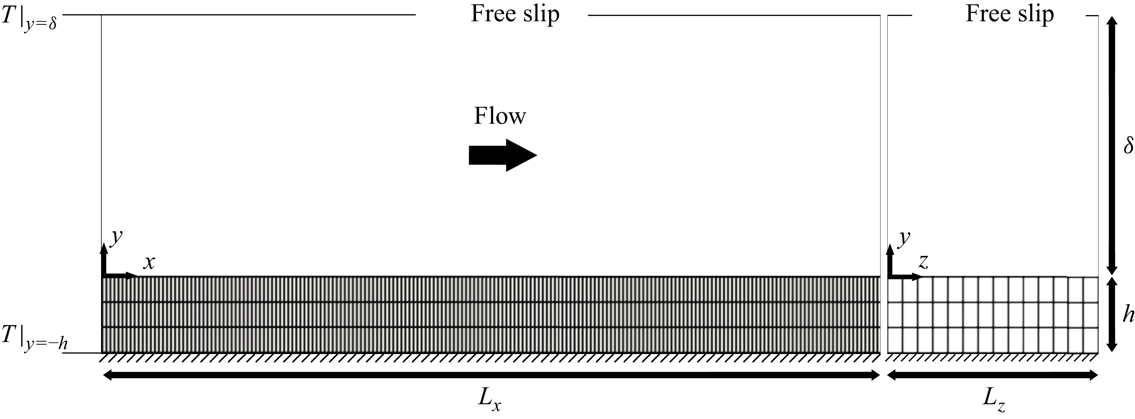

 sx+
sx+ sy+
sy+ sz+
sz+ Kx+
Kx+ Ky+
Ky+ Kz+
Kz+ ReK
ReK

 −−
−− −−
−− ⋅⋅⋅
⋅⋅⋅ ∘
∘
 y=0
y=0 uτ
uτ KP1a
KP1a KP1b
KP1b KP2a
KP2a KP2b
KP2b KP3a
KP3a KP3b
KP3b
 y=0
y=0 uτ
uτ KP1a
KP1a KP1b
KP1b KP2a
KP2a KP2b
KP2b KP3a
KP3a KP3b
KP3b
 kx+kz+Euu+
 kx+kz+Evv+
 kx+kz+Euv+
 y=0
y=0 KP1b
KP1b KP1a
KP1a KP1
KP1 SP
SP KP1b,
KP1b, kx+kz+Euu+
 KP1b,
KP1b, kx+kz+Evv+
 KP1b,
KP1b, kx+kz+Euv+
 KP1a,
KP1a, kx+kz+Euu+
 KP1a,
KP1a, kx+kz+Evv+
 KP1a,
KP1a, kx+kz+Euv+
 KP1,
KP1, kx+kz+Euu+
 KP1,
KP1, kx+kz+Evv+
 KP1,
KP1, kx+kz+Euv+
 SP,
SP, kx+kz+Euu+
 SP,
SP, kx+kz+Evv+
 SP,
SP, kx+kz+Euv+


 y=0
y=0 KP1a
KP1a KP1b
KP1b
 kx+kz+Eθθ+
 kx+kz+Eθv+
 y=0
y=0 KP1,
KP1, kx+kz+Eθθ+
 KP1a,
KP1a, kx+kz+Eθθ+
 KP1b,
KP1b, kx+kz+Eθθ+
 KP1,
KP1, kx+kz+Eθv+
 KP1a,
KP1a, kx+kz+Eθv+
 KP1b,
KP1b, kx+kz+Eθv+
 SP,
SP, kx+kz+Eθθ+
 TP,
TP, kx+kz+Eθθ+
 SP,
SP, kx+kz+Eθv+
 TP,
TP, kx+kz+Eθv+

 y=0
y=0
 St
St Kx+Ky+
 u′
u′ v′
v′ θ′
θ′ v′
v′
 θ′v′
θ′v′ u′v′
u′v′ y=0
y=0 KP1b
KP1b KP1a
KP1a KP1
KP1 TP
TP SP
SP |θ′v′|=8×θ′v′¯
 |u′v′|=8×−u′v′¯
 Ub
Ub
 Open access

