





1. Introduction
The ice mass within glaciers, ice sheets and icebergs constitutes an important but delicate component of the global energy balance. Small changes in ice mass fluxes can have large impacts far beyond the high-latitude regions where this ice predominantly resides. In ice–ocean interactions, the ice melt occurring at this interface is typically controlled by the fluid motion of the adjacent ocean water. Du, Calzavarini & Sun (Reference Du, Calzavarini and Sun2024) provide a useful review on the recently developed laboratory, computational and theoretical tools being used to study this coupled process from a fundamental fluid mechanical perspective, and how the results can be connected with processes that occur at the larger, geophysical scales relevant for climate models.
Of the myriad processes occurring at the ice–ocean interface, we focus here on how surface gravity waves can erode the sidewalls of icebergs, the faces of marine- and freshwater-terminating glaciers, and the calving fronts of ice shelves. The efficacy with which wave-induced melt transpires depends on environmental factors that vary widely between different settings: the amplitude and period of the incoming waves; whether the ice face is exposed to non-breaking or breaking waves; the stratification and temperature profiles of the adjacent water; whether the water surface is open or covered by sea ice or an ice mélange; and the material integrity and geometric configuration of the ice face itself. However, how each of these impact the erosion rate remains poorly understood. Challenges to studying this process include: in situ observations of ice cliffs are costly, cumbersome and risky; laboratory investigations require careful control of ice, water and wave conditions, ideally at cold ambient temperatures; and theoretical progress is made difficult by the complex interactions at the ice–water interface, with confounding roles of temperature, salinity and wave action.
From observations, we know that wave-driven erosion is typically maximised for icebergs floating in the open ocean, particularly once they have drifted to lower latitudes. At the other end of the spectrum, wave action is largely suppressed in mélange-choked fjords. However, conditions can quickly change, such as when loss of sea ice exposes the glacier or ice-shelf front to open water, allowing wave erosion to become an important factor in determining calving rates. Wave-induced erosion has historically been partitioned into three main processes (Savage Reference Savage2001): (i) wave-induced melt resulting in incision near the waterline; (ii) calving of the above-water section of the ice cliff that overhangs the waterline incision; (iii) submerged or full-depth calving due to buoyant forces on underwater ice benches (or ‘feet’), produced by the collapse of the above-water cliff, that can protrude of the order of 100 m beyond the overhang (‘footloose’-style, notch-triggered buoyant calving, e.g. Wagner et al. Reference Wagner, Wadhams, Bates, Elosegui, Stern, Vella, Abrahamsen, Crawford and Nicholls2014; Benn et al. Reference Benn, Ångström, Zwinger, Todd, Nick, Cook, Hulton and Luckman2017; Trevers et al. Reference Trevers, Payne, Cornford and Moon2019). Both (ii) and (iii) respond directly to the rate of the wave-induced melt (i) and hence should scale with it, making this particular melt process a potential key driver of ice loss for icebergs, glaciers and ice shelves.
Definition sketch for non-breaking surface waves reflecting at an ice wall. The wall is initially located at $x=0$
, with the mean water level at
$x=0$
, with the mean water level at $z=0$
. Waves of amplitude
$z=0$
. Waves of amplitude $a$
(peak-to-peak oscillation of
$a$
(peak-to-peak oscillation of $2a$
) and wavenumber
$2a$
) and wavenumber $k$
strike the ice wall and reflect back to create a standing wave pattern with amplitude
$k$
strike the ice wall and reflect back to create a standing wave pattern with amplitude $2a$
(peak-to-peak oscillation of
$2a$
(peak-to-peak oscillation of $4a$
). The ice wall melts and the evolving ice face position is described by
$4a$
). The ice wall melts and the evolving ice face position is described by $m(z,t)$
.
$m(z,t)$
.

Here, we consider an idealised set-up of the problem from both theoretical and experimental points of view (figure 1), which does not represent a particular geophysical setting but rather is concerned with the fundamental interaction between surface waves and a vertical ice face. In this idealised set-up, to make the problem more tractable, we focus on: (i) freshwater at constant density, ignoring the role of salinity and only including buoyancy effects due to temperature variations of the water in so far as they effect the ambient melt without waves, and (ii) non-breaking waves that strike an ice cliff and reflect back, creating standing waves.
Quantifying wave-driven ice erosion in this set-up requires understanding of the heat flux across the unsteady and often turbulent boundary layers generated by the oscillatory flow in surface waves. Faced with this difficult task, one approach is to approximate the oscillatory flow as quasi-steady and use known relationships between flow velocity and heat flux in steady flow. There are a number of empirical correlations and approximate theories to relate heat flux and flow velocity for the canonical situation of zero-pressure-gradient, steady and turbulent boundary layer flow over a smooth surface (e.g. Eckert & Drake Reference Eckert and Drake1959; Kader & Yaglom Reference Kader and Yaglom1972; White Reference White1974; Bird, Stewart & Lightfoot Reference Bird, Stewart and Lightfoot2007). They all tend to predict a heat transfer coefficient that scales linearly with the average, steady velocity (or near linearly due to a weak dependency on the Reynolds number). As a result, existing parameterisations of ice erosion often predict an ice melt rate that scales linearly (or near linearly) with the flow velocity. Examples of such linear-with-velocity ice melt rate scalings include those introduced in Weeks & Campbell (Reference Weeks and Campbell1973), White, Spaulding & Gominho (Reference White, Spaulding and Gominho1980) and Holland & Jenkins (Reference Holland and Jenkins1999). Many studies have subsequently used those expressions for wave erosion of ice (e.g. El-Tahan, Venkatesh & El-Tahan Reference El-Tahan, Venkatesh and EL-Tahan1987; Kubat, Sayed & Savage Reference Kubat, Sayed and Savage2007; Anselin et al. Reference Anselin, Reed, Jenkins and Green2023; Crawford et al. Reference Crawford, Crocker, Smith, Mueller and Wagner2024; Sweetman, Shakespeare & Stewart Reference Sweetman, Shakespeare and Stewart2025; Mamer & Robel Reference Mamer and Robel2026).
While there is good evidence for this linear scaling in steady flows (e.g. see figure 13.4-2 in Bird et al. Reference Bird, Stewart and Lightfoot2007), there is little reason to believe it should translate to the highly unsteady flow in wavy conditions. A dimensionless measure of how well an oscillatory flow interacting with a solid body can be approximated as quasi-steady is given by the Keulegan–Carpenter number (e.g. Dalrymple & Dean Reference Dalrymple and Dean1991, Ch. 8.3), and computing this number shows that wave erosion of ice cliffs does not fall into the quasi-steady regime. Indeed, Weiss et al. (Reference Weiss, Nash, Wengrove, Osman, Cohen, Jackson, Pettit, Zhao, Nahorniak and Sutherland2025) recently reported field data that show how flow unsteadiness can cause the melt rates to be severely under-predicted by parameterisations that assume steady flow. Their findings echo analogous work on solid bodies, where unsteady flow due to waves was found to cause a significant enhancement of mass transfer and dissolution of a solid body relative to steady flow conditions with the same velocity magnitude (Reidenbach et al. Reference Reidenbach, Koseff, Monismith, Steinbuckc and Genin2006, Reference Reidenbach, Koseff and Monismith2007).
On a related note, the onset and role of turbulence in oscillatory boundary layers can be subtle. For example, the transition to turbulence in oscillatory flows is phase dependent, i.e. certain phases of the cycle will show turbulent features before others, and the phase lags between boundary layer flow and free-stream flow are different in fully turbulent conditions compared with laminar ones. Additionally, typical laboratory experiments of wave erosion on ice will use wave periods of 0.5–1 s and wave amplitudes of 1–3 cm in water depths of 25–50 cm (see table 4.1 in Wolterman Reference Wolterman2025, for a list of previous work on the topic), but oscillatory boundary layers associated with these wave conditions do not surpass the Reynolds number threshold for laminar-to-turbulence transition (Jensen, Sumer & Fredsøe Reference Jensen, Sumer and Fredsøe1989). This means that it is difficult to test theories that assume fully turbulent field conditions on typical laboratory scales, and conversely, difficult to calibrate turbulent transport coefficients in typical laboratory settings for application to fully turbulent field conditions.
Lastly, an important aspect of quantifying the heat flux across oscillatory boundary layers is that such flows can produce wave-averaged currents through a variety of mechanisms. First, when oscillatory flow is imposed adjacent to a solid boundary where the amplitude or phase of the oscillation varies in the flow-parallel direction, the boundary layer dynamics produces a small but unidirectional wave-averaged current in an effect known as boundary layer streaming (e.g. Rayleigh Reference Rayleigh1884; Longuet-Higgins Reference Longuet-Higgins1953; Hunt & Johns Reference Hunt and Johns1963). The importance of the streaming current lies in the fact that, although it is small, it leads to a net transport of heat in a specific direction even though the imposed oscillatory flow oscillates in both directions with equal magnitude. Additionally, in laboratory settings, the finite size of wave tanks means that the streaming flow (and other mechanisms that produce a net movement of water, such as Stokes drift) must be balanced by return flows elsewhere (Swan Reference Swan1990; Bremer & Breivik Reference Bremer and Breivik2017), potentially resulting in a large-scale recirculation that may impact the net heat flux to any ice within the tank. Second, if a solid body of ice is oscillated in otherwise quiescent water instead of oscillatory flow generated by waves striking the ice (e.g. Sweetman et al. Reference Sweetman, Shakespeare and Stewart2025), the inertial response of the fluid typically results in a slow, cycle-averaged pumping of the fluid away from the body in the directions of oscillation. This pumping, together with the need to conserve mass, draws fluid inwards laterally and sets up recirculation cells whose number, size, speed and geometry all depend on the solid body, the imposed oscillations and the tank geometry (e.g. Blum et al. Reference Blum, Kunwar, Johnson and Voth2010; Laurent et al. Reference Laurent, La Ragione, Jenkins and Bewley2022).
Regarding previous work, White et al. (Reference White, Spaulding and Gominho1980) is considered the prevailing parameterisation of wave-induced melting of ice cliffs. Their melt rate parameterisation presupposes White’s (Reference White1974) theory of relating heat flux to momentum flux in a steady, turbulent boundary layer flow can be combined with an empirical correlation between the friction coefficient and the local Reynolds number for oscillatory flows. Thus, their parameterisation implicitly assumes steady and fully turbulent flow, even if part of the derivation considers wave-driven oscillatory flow. There is scant previous work in terms of laboratory experiments, but White et al. (Reference White, Spaulding and Gominho1980) do report two wave-induced ice melting experiments in relatively warm freshwater without noting waterline melt rates. Daley & Veitch (Reference Daley and Veitch2000) also report several similar experiments, but with insufficient detail to infer the precise conditions and waterline erosion rates. Martin, Josberger & Kauffman (Reference Martin, Josberger and Kauffman1978) reported an experiment with waves of period 0.4 s and amplitude 2.5 cm generated in a wave tank with a water depth of 40 cm at a uniform oceanic salinity (34 psu) and low ambient water temperature ( $4\,^\circ \text{C}$
); they measured a wave-induced notch that extended approximately 4 cm above the waterline, 11 cm below and 8 cm into the ice block after 45 min. While White et al.’s parameterisation appears to give good predictions with the little laboratory data available, the agreement is likely to be a coincidence since these laboratory experiments are not in fully turbulent conditions. This would then also explain why field estimates of the wave-driven melt rate reported in Martin et al. (Reference Martin, Josberger and Kauffman1978) and Keys & Williams (Reference Keys and Williams1984) are much smaller than the values calculated with White et al.’s parameterisation.
$4\,^\circ \text{C}$
); they measured a wave-induced notch that extended approximately 4 cm above the waterline, 11 cm below and 8 cm into the ice block after 45 min. While White et al.’s parameterisation appears to give good predictions with the little laboratory data available, the agreement is likely to be a coincidence since these laboratory experiments are not in fully turbulent conditions. This would then also explain why field estimates of the wave-driven melt rate reported in Martin et al. (Reference Martin, Josberger and Kauffman1978) and Keys & Williams (Reference Keys and Williams1984) are much smaller than the values calculated with White et al.’s parameterisation.
We conclude that existing representations of wave-induced sidewall erosion of ice cliffs lack a thorough theoretical examination of the heat transport in oscillatory flows and a careful comparison against field and laboratory data. In order to constrain the broad question of how waves erode ice cliffs, we present results from laboratory experiments and corresponding theoretical considerations that are made tractable by focusing on the idealised set-up described above and shown in figure 1. We show that good agreement can be achieved between laboratory experiments and theoretical predictions based on the hypothesis that heat transport is primarily governed by the balance between advective vertical transport by a wave-averaged boundary layer streaming current and horizontal transport by diffusion. This suggests that these fundamental processes are also likely to play a key role in setting real-world erosion rates.
In the remainder of the paper, we first present our theory of wave-induced melt of ice cliffs, including a new formulation for the predicted melt rate (§ 2), followed by laboratory experiments and their results (§ 3) and the implications of our work for geophysical and climate models (§ 4). We end with brief conclusions and directions for future work (§ 5).
2. Theory
2.1. Standing waves at an ice cliff
For planar, deep-water, small-amplitude surface gravity waves reflecting off a vertical ice wall (figure 1), the inviscid and irrotational solutions to the free-surface displacement and velocity field can be constructed from a superposition of progressive waves travelling in opposite directions (e.g. Dalrymple & Dean Reference Dalrymple and Dean1991; Mei, Stiassnie & Yue Reference Mei, Stiassnie and Yue2005). This solution is given by the real parts of
 \begin{align} \phi &= \mathrm{i}g\frac {2a}{\omega }e^{kz}\cos kx\,e^{\mathrm{i}\omega t}, \\[-12pt]\nonumber \end{align}
 \begin{align} \eta &= -\frac {1}{g}\frac {\partial \phi }{\partial t}\bigg |_{z=0}=2a\cos kx\,e^{\mathrm{i}\omega t}, \\[-12pt]\nonumber \end{align}
 \begin{align} u_I &= \frac {\partial \phi }{\partial x}=-\mathrm{i}g\frac {2ka}{\omega }e^{kz}\sin kx\,e^{\mathrm{i}\omega t}, \\[-12pt]\nonumber \end{align}
 \begin{align} w_I &= \frac {\partial \phi }{\partial z}=\mathrm{i}g\frac {2ka}{\omega }e^{kz}\cos kx\,e^{\mathrm{i}\omega t}, \end{align}
where $\phi$
is the velocity potential,
$\phi$
is the velocity potential, $\eta$
is the free-surface displacement and
$\eta$
is the free-surface displacement and $u_I,w_I$
are the horizontal and vertical velocities, respectively. The subscript
$u_I,w_I$
are the horizontal and vertical velocities, respectively. The subscript $I$
emphasises that this is the inviscid and irrotational flow solution. The waves are characterised by angular frequency
$I$
emphasises that this is the inviscid and irrotational flow solution. The waves are characterised by angular frequency $\omega$
and wavenumber
$\omega$
and wavenumber $k$
, which follow the deep-water dispersion relation
$k$
, which follow the deep-water dispersion relation $\omega ^2 =gk$
, where
$\omega ^2 =gk$
, where $g$
is the gravitational acceleration. The incident waves have an amplitude
$g$
is the gravitational acceleration. The incident waves have an amplitude $a$
, which means the free surface oscillates between
$a$
, which means the free surface oscillates between $-2a$
and
$-2a$
and $+2a$
at the anti-nodes in pure standing waves.
$+2a$
at the anti-nodes in pure standing waves.
2.2. Wave-averaged heat transport in the ice-adjacent boundary layer
To develop a theory of wave-induced ice melt, we use the passive scalar heat transport equation
 \begin{equation} \frac {\partial \theta }{\partial t}+u\frac {\partial \theta }{\partial x}+w\frac {\partial \theta }{\partial z}=\alpha\! \left(\frac {\partial ^2\theta }{\partial x^2}+\frac {\partial ^2\theta }{\partial z^2}\right)\!, \end{equation}
where $\theta$
is the temperature,
$\theta$
is the temperature, $(u,w)$
is the fluid velocity field and
$(u,w)$
is the fluid velocity field and $\alpha$
is the thermal diffusivity of the fluid. By treating temperature as a passive scalar, we ignore the feedback between temperature and fluid density that would result in buoyancy-driven natural convection flows. We neglect these effects for the sake of simplicity in order to focus on the wave-induced heat transport and melt, and then evaluate their importance a posteriori in laboratory data (§ 3).
$\alpha$
is the thermal diffusivity of the fluid. By treating temperature as a passive scalar, we ignore the feedback between temperature and fluid density that would result in buoyancy-driven natural convection flows. We neglect these effects for the sake of simplicity in order to focus on the wave-induced heat transport and melt, and then evaluate their importance a posteriori in laboratory data (§ 3).
In principle, (2.2) can be solved using (2.1) with appropriate temperature boundary conditions. However, the wave-induced erosion of the ice will be strongly influenced by the dynamics and transport in the boundary layer near the ice–water interface. Furthermore, the flow described by the inviscid and irrotational solution in (2.1) is only an adequate description of the wave-driven flow outside the boundary layer, since the flow within the boundary layer is affected by viscosity and includes rotational velocities.
Oscillatory boundary layer flow is a classical problem in fluid mechanics, and the solution for the boundary layer flow due the reflection of surface waves from a vertical wall can be readily obtained from canonical analogous solutions (Batchelor Reference Batchelor2000; Kundu, Cohen & Dowling Reference Kundu, Cohen and Dowling2012). These solutions show that the leading-order flow field in boundary layers driven by oscillatory flow remains oscillatory, albeit modified by viscous effects. In terms of scalar transport, this oscillatory flow only serves to cause oscillatory advection with no net transport. However, oscillatory boundary layers can also produce Lagrangian mass transport at second order that can result in a net advection of passive scalars (Rayleigh Reference Rayleigh1884; Batchelor Reference Batchelor2000). In particular, it has been shown that the boundary layer flow of surface waves interacting with a wall produces a wall-parallel Eulerian streaming current (Hunt & Johns Reference Hunt and Johns1963; Mei et al. Reference Mei, Stiassnie and Yue2005), and that such a current is an important component of the wave-averaged scalar transport dynamics where the effects of wave-induced oscillations have been averaged out (Mei & Chian Reference Mei and Chian1994; Winckler, Liu & Mei Reference Winckler, Liu and Mei2013; Michele et al. Reference Michele, Stuhlmeier and Borthwick2021, Reference Michele, Borthwick and van den Bremer2023).
Since the boundary layer flow and the corresponding passive scalar transport equations for surface waves reflecting at a vertical wall do not appear to have been previously published, we provide a full derivation in Appendix A. To summarise it here, we use a multi-time-scale expansion to isolate the slow, wave-averaged dynamics from the fast, wave-resolved dynamics. This procedure yields a wave-averaged advection–diffusion equation for the temperature, where the advection consists of both Eulerian current and Stokes drift terms and where the horizontal diffusion dominates over the vertical because of the large gradients in the wall-normal direction across the boundary layer. For wave-induced melt of an ice cliff, we also show how the same multi-time-scale expansion can be used to derive a wave-averaged Stefan condition that reduces the wave-averaged transport equation to a boundary value problem. Solving this boundary value problem gives the wave-averaged temperature field which can then be inserted back into the wave-averaged Stefan condition to compute the wave-averaged melt rate.
Here, we solve a simplified, approximate version of the full problem that is derived in Appendix A. Specifically, we focus on how the wave-averaged temperature field is controlled by the balance between vertical advection by the Eulerian streaming current and horizontal diffusion. This simplified balance can be written as
 \begin{equation} W \frac {\partial \varTheta }{\partial z} = \alpha \frac {\partial ^2\varTheta }{\partial x^2}, \end{equation}
where the capital variables $W$
and
$W$
and $\varTheta$
signify wave-averaged versions of
$\varTheta$
signify wave-averaged versions of $w$
and
$w$
and $\theta$
, respectively. For
$\theta$
, respectively. For $W$
, we use the expression from Batchelor (Reference Batchelor2000) for the Eulerian streaming current at the edge of the boundary layer that bypasses the need for a full multi-time-scale analysis (see his equation (5.13.20)). For our case, Batchelor’s expression simplifies to
$W$
, we use the expression from Batchelor (Reference Batchelor2000) for the Eulerian streaming current at the edge of the boundary layer that bypasses the need for a full multi-time-scale analysis (see his equation (5.13.20)). For our case, Batchelor’s expression simplifies to
 \begin{equation} W = -\frac {3}{8\omega } \frac {\rm d}{{\rm d}z}\big (w_I(x=0) \, w_I^*(x=0)\big ) = - 3 \frac {\omega }{k} (ka)^2 e^{2kz}, \end{equation}
where the $^*$
denotes a complex conjugate. This expression, which is consistent with our full solution in Appendix A, is independent of the viscosity, which means that it would also remain valid in turbulent conditions under the assumption of a constant turbulent viscosity.
$^*$
denotes a complex conjugate. This expression, which is consistent with our full solution in Appendix A, is independent of the viscosity, which means that it would also remain valid in turbulent conditions under the assumption of a constant turbulent viscosity.
Before presenting the solution, we summarise the problem in dimensionless terms. We introduce the dimensionless variables
 \begin{equation} \begin{aligned} x \rightarrow \delta \frac {1}{k}\xi , \, z \rightarrow \frac {1}{k}z, W \rightarrow \frac {\omega }{k}W, \, \varTheta \rightarrow (\theta _w-\theta _m)\varTheta + \theta _m , \end{aligned} \end{equation}
where $\theta _m$
is the melting temperature of the ice and
$\theta _m$
is the melting temperature of the ice and $\theta _w$
is the ambient water temperature. We have introduced a stretched coordinate
$\theta _w$
is the ambient water temperature. We have introduced a stretched coordinate $\xi$
for the wall-normal horizontal direction based on the boundary layer thickness, which is expected to be
$\xi$
for the wall-normal horizontal direction based on the boundary layer thickness, which is expected to be $O(\sqrt {\nu /\omega })$
; therefore,
$O(\sqrt {\nu /\omega })$
; therefore, $\delta = \sqrt {k^2\nu /\omega }$
is the dimensionless boundary layer thickness. The equation to solve then becomes
$\delta = \sqrt {k^2\nu /\omega }$
is the dimensionless boundary layer thickness. The equation to solve then becomes
 \begin{equation} W \frac {\partial \varTheta }{\partial z} = {\textit{Pr}}^{-1}\frac {\partial ^2\varTheta }{\partial \xi ^2}, \end{equation}
where $W = - 3 \varepsilon ^2 e^{2z}$
is the dimensionless advection velocity, with
$W = - 3 \varepsilon ^2 e^{2z}$
is the dimensionless advection velocity, with $\varepsilon = ka$
being the wave steepness and
$\varepsilon = ka$
being the wave steepness and $Pr = \nu /\alpha$
being the Prandtl number. This equation applies only in the region near the surface where the influence of the waves is of leading-order importance, i.e. at depths given by
$Pr = \nu /\alpha$
being the Prandtl number. This equation applies only in the region near the surface where the influence of the waves is of leading-order importance, i.e. at depths given by $-z = O(1)$
or smaller.
$-z = O(1)$
or smaller.
The boundary conditions are
 \begin{align} \varTheta (\xi =0) &= 0, \\[-12pt]\nonumber \end{align}
 \begin{align} \varTheta (\xi \rightarrow \infty ) &= 1, \\[-12pt]\nonumber \end{align}
 \begin{align} \frac {{\rm d}M}{{\rm d}T} &= - \left(\frac{\rho}{\rho_\textit{ice}}\right){\textit{Ste}} \, {\textit{Pr}}^{-1} \frac {\partial \varTheta }{\partial \xi } \bigg \lvert _{\xi =0}, \end{align}
where $M$
is the wave-averaged position of the ice–water interface,
$M$
is the wave-averaged position of the ice–water interface, $({\rho}/{\rho_\textit{ice}})$
is the water-to-ice density ratio, and
$({\rho}/{\rho_\textit{ice}})$
is the water-to-ice density ratio, and ${\textit{Ste}} = c_{\!p} \lvert \theta _w - \theta _m \lvert /L$
is the Stefan number, with
${\textit{Ste}} = c_{\!p} \lvert \theta _w - \theta _m \lvert /L$
is the Stefan number, with $c_{\!p}$
being the specific heat capacity of the water and
$c_{\!p}$
being the specific heat capacity of the water and $L$
being the latent heat of fusion of the ice. Here, (2.7a
) and (2.7b
) specify that the wave-averaged temperature must equal the melting temperature at the ice wall and recover to the ambient water temperature far outside the boundary layer. Equation (2.7c
) is the wave-averaged Stefan condition assuming water-side dominance in the heat transfer, which sets the melt rate (derived in Appendix A).
$L$
being the latent heat of fusion of the ice. Here, (2.7a
) and (2.7b
) specify that the wave-averaged temperature must equal the melting temperature at the ice wall and recover to the ambient water temperature far outside the boundary layer. Equation (2.7c
) is the wave-averaged Stefan condition assuming water-side dominance in the heat transfer, which sets the melt rate (derived in Appendix A).
In summary, we must solve (2.6) subject to boundary conditions (2.7a
) and (2.7b
) to obtain the wave-averaged temperature solution, and then use this solution to evaluate the wave-averaged melt rate using (2.7c
). The relevant dimensionless parameters are again the wave steepness $\varepsilon = ka$
, the dimensionless boundary layer thickness
$\varepsilon = ka$
, the dimensionless boundary layer thickness $\delta = \sqrt {k^2\nu /\omega }$
, the inverse Prandtl number
$\delta = \sqrt {k^2\nu /\omega }$
, the inverse Prandtl number $\textit{Pr} ^{-1} = \alpha /\nu$
and the Stefan number
$\textit{Pr} ^{-1} = \alpha /\nu$
and the Stefan number ${\textit{Ste}} = c_{\!p} \lvert \theta _w - \theta _m \lvert /L$
, all of which tend to be small (see Appendix A for more details).
${\textit{Ste}} = c_{\!p} \lvert \theta _w - \theta _m \lvert /L$
, all of which tend to be small (see Appendix A for more details).
2.3. Wave-averaged temperature field and melt rate
Physically, (2.6) states that a downward advection of temperature whose strength scales with the square of the wave steepness and decays exponentially with depth must balance the horizontal diffusion. The solution to such a problem can be found in terms of similarity variables, analogous to canonical boundary layer solutions (see the Blasius and Falkner–Skan solutions in, e.g. Kundu et al. Reference Kundu, Cohen and Dowling2012).
First, we introduce a new vertical coordinate
 \begin{align} \zeta = e^z, \end{align}
so that the advection velocity becomes $-3\varepsilon ^2 \zeta ^{2}$
, as well as
$-3\varepsilon ^2 \zeta ^{2}$
, as well as $\partial / \partial z \rightarrow \zeta \partial /\partial \zeta$
. Now, the equation to solve is
$\partial / \partial z \rightarrow \zeta \partial /\partial \zeta$
. Now, the equation to solve is
 \begin{equation} -3\varepsilon ^2 \zeta ^{3} \frac {\partial \varTheta }{\partial \zeta } = {\textit{Pr}}^{-1}\frac {\partial ^2\varTheta }{\partial \xi ^2}. \end{equation}
We propose that the similarity solution
 \begin{equation} \varTheta = F(\chi ), \ \text{ where } \ \chi = \frac {\xi }{\varDelta } \end{equation}
is the similarity variable. Here, $\varDelta = \varDelta (\zeta )$
corresponds to the thermal boundary layer thickness. Inserting (2.10) into (2.9) gives
$\varDelta = \varDelta (\zeta )$
corresponds to the thermal boundary layer thickness. Inserting (2.10) into (2.9) gives
 \begin{equation} 3\varepsilon ^2 \zeta ^{3} F^{\prime } \chi \frac {\varDelta ^{\prime }}{\varDelta } = {\textit{Pr}}^{-1}\frac {F^{\prime \prime }}{\varDelta ^2}, \end{equation}
where the prime denotes differentiation. The introduction of the similarity variable has turned the partial differential equation into an ordinary differential equation, allowing us to rearrange the equation to have all terms that are functions of $\chi$
on the left side and all terms that are functions of
$\chi$
on the left side and all terms that are functions of $\zeta$
on the right side. Then, since
$\zeta$
on the right side. Then, since $\chi$
and
$\chi$
and $\zeta$
are independent, each side must in turn be equal to a constant. Doing so gives
$\zeta$
are independent, each side must in turn be equal to a constant. Doing so gives
 \begin{equation} \frac {1}{3\varepsilon ^2 {\textit{Pr}}} \frac {F^{\prime \prime }}{F^{\prime }} \frac {1}{\chi } = \varDelta ^{\prime } \varDelta \zeta ^3 = -C, \end{equation}
where the negative sign of $C$
comes from inspection of the sign of
$C$
comes from inspection of the sign of $\varDelta ^{\prime }$
– the thickness of the temperature boundary layer must increase with depth below the surface since the advective velocity decreases in magnitude with depth.
$\varDelta ^{\prime }$
– the thickness of the temperature boundary layer must increase with depth below the surface since the advective velocity decreases in magnitude with depth.
We first tackle the right side of the equation to find $\varDelta$
and uncover the form of the similarity variable. We find that it can be written as
$\varDelta$
and uncover the form of the similarity variable. We find that it can be written as
 \begin{align} \frac {{\rm d} \left ( \frac {1}{2}\varDelta ^2 \right )}{{\rm d}\zeta } = -\frac {C}{\zeta ^3}, \end{align}
which can be integrated to give
 \begin{align} \varDelta ^2 = C\zeta ^{-2}, \end{align}
or with a choice of $C=1$
$C=1$
 \begin{align} \varDelta = \zeta ^{-1}. \end{align}
This means that $\varDelta = e^{-z}$
, which shows that the thermal boundary layer thickness increases exponentially with depth to match the exponential decrease in the magnitude of the wave-induced velocity. It also means that the final form of the similarity variable is
$\varDelta = e^{-z}$
, which shows that the thermal boundary layer thickness increases exponentially with depth to match the exponential decrease in the magnitude of the wave-induced velocity. It also means that the final form of the similarity variable is
 \begin{equation} \chi = \xi \zeta. \end{equation}
We now turn to the left side of the equation to find the solution for $F$
. With the choice of
$F$
. With the choice of $C=1$
already made, we must solve the ordinary differential equation
$C=1$
already made, we must solve the ordinary differential equation
 \begin{align} F^{\prime \prime } + 3 \varepsilon ^2 {\textit{Pr}} \, \chi F^{\prime } = 0. \end{align}
We let $f = F^{\prime }$
to rewrite this equation as
$f = F^{\prime }$
to rewrite this equation as
 \begin{align} f^{\prime } + 3 \varepsilon ^2 {\textit{Pr}} \, \chi f = 0. \end{align}
This is a first-order ordinary differential equation that can be solved with an integrating factor, producing the following solution:
 \begin{align} \exp {\left ( \frac {3}{2} \varepsilon ^2 {\textit{Pr}} \, \chi ^2 \right )}f = C_1, \end{align}
where $C_1$
is a constant of integration. Inserting
$C_1$
is a constant of integration. Inserting $f = F^{\prime }$
then gives
$f = F^{\prime }$
then gives
 \begin{align} F^{\prime } = C_1 \exp {\left (- \frac {3}{2} \varepsilon ^2 {\textit{Pr}} \, \chi ^2 \right )}, \end{align}
whose integral can be written in terms of error functions as
 \begin{align} F = C_1 \left [ \frac {\sqrt {\pi }}{2} \frac { \mathrm{erf} \left ( \sqrt { (3/2) {\textit{Pr}} } \, \varepsilon \chi \right ) }{\sqrt {(3/2) {\textit{Pr}} } \, \varepsilon \, } \right ] + C_2, \end{align}
where $C_2$
is another constant of integration.
$C_2$
is another constant of integration.
The boundary conditions in terms of the similarity variables become $F(\chi = 0) = 0$
and
$F(\chi = 0) = 0$
and $F(\chi \rightarrow \infty ) = 1$
. From the first boundary condition, we get
$F(\chi \rightarrow \infty ) = 1$
. From the first boundary condition, we get $C_2 = 0$
. From the second boundary condition, we find
$C_2 = 0$
. From the second boundary condition, we find
 \begin{align} C_1 = \frac {2}{\sqrt {\pi }}\sqrt {\frac {3}{2} {\textit{Pr}} } \, \varepsilon . \end{align}
Thus, the final similarity solution is
 \begin{align} F = \mathrm{erf}\left ( \sqrt {\frac {3}{2} {\textit{Pr}} } \, \varepsilon \chi \right )\!, \end{align}
which when written in terms of the original dimensionless variables is
 \begin{equation} \varTheta = \mathrm{erf} \left ( \sqrt {\frac {3}{2} {\textit{Pr}} } \, \varepsilon \, \xi \, e^{z} \right )\!. \end{equation}
This solution for the wave-averaged temperature field is plotted in figure 2, showing how the downward advection draws the warmer water closer to the ice, with this effect being strongest at the surface and decaying with depth. This solution only applies to depths where the influence of waves is important, i.e. $-z = O(1)$
or smaller.
$-z = O(1)$
or smaller.
Wave-averaged temperature $\varTheta$
plotted against horizontal distance away from the ice–water interface
$\varTheta$
plotted against horizontal distance away from the ice–water interface $\xi$
and depth below the water surface
$\xi$
and depth below the water surface $z$
for wave steepness
$z$
for wave steepness $\varepsilon =0.25$
and Prandtl number
$\varepsilon =0.25$
and Prandtl number $Pr = 5$
using (2.24).
$Pr = 5$
using (2.24).

Inserting (2.24) into (2.7c ) gives the dimensionless wave-induced melt rate profile
 \begin{equation} \frac {{\rm d}M}{{\rm d}T} = \sqrt {\frac {6}{\pi }}\,\left(\frac{\rho}{\rho_\textit{ice}}\right)\,{\textit{Ste}} \, {\textit{Pr}}^{-1/2} \, \varepsilon \, e^z, \end{equation}
where we have dropped the negative sign with the understanding that this melt rate indicates the rate at which the ice–water interface moves into the ice.
In dimensional form, the melt rate profile is given by
 \begin{equation} \frac {\mathrm{d}m}{\mathrm{d}t} = \sqrt {\alpha \omega } \, \sqrt { \frac {6}{\pi } }\,\left(\frac{\rho}{\rho_\textit{ice}}\right)\, \frac {c_{\!p} \lvert \theta _w - \theta _m \lvert }{L} \, ka \, e^{kz} = \left ( \sqrt { \frac {6 \alpha }{\pi }}\,\frac{\rho}{\rho_\textit{ice}}\, \frac {c_{\!p}}{gL} \right ) \, a \, \omega ^{5/2} \, \lvert \theta _w - \theta _m \rvert \, e^{kz} , \end{equation}
where the first expression emphasises the melt rate scaling and the second expression isolates constants and material properties from the relevant environmental conditions. At the waterline ( $z=0$
), the melt rate is given by
$z=0$
), the melt rate is given by
 \begin{equation} \frac {\mathrm{d}m}{\mathrm{d}t} \bigg \rvert _{z=0} = \left ( \sqrt { \frac {6 \alpha }{\pi }}\,\frac{\rho}{\rho_\textit{ice}} \, \frac {c_{\!p} }{gL} \right ) \, a \, \omega ^{5/2} \, \lvert \theta _w - \theta _m \rvert . \end{equation}
The depth-integrated melt rate, which quantifies the rate of loss of ice volume per unit spanwise length, is given by
 \begin{equation} \int _{-\infty }^0 \frac {\mathrm{d}m}{\mathrm{d}t} \, {\rm d}z = \sqrt {\alpha \omega } \, \sqrt { \frac {6}{\pi } } \,\left(\frac{\rho}{\rho_\textit{ice}}\right)\, \frac {c_{\!p} \lvert \theta _w - \theta _m \lvert }{L} \, a = \left ( \sqrt { \frac {6 \alpha }{\pi } }\,\frac{\rho}{\rho_\textit{ice}} \frac {c_{\!p}}{L} \right ) \, a \omega ^{1/2} \, \lvert \theta _w - \theta _m \lvert , \end{equation}
where, again, the first expression emphasises the melt rate scaling and the second expression isolates constants and material properties from the relevant environmental conditions.
2.4. Interpretation of theoretical results
In our theory, the near-ice temperature field is set by a balance of vertical heat transport by boundary layer streaming and horizontal heat transport by diffusion. Since the streaming velocity decays with depth, the thermal boundary layer thickens with depth, and this sets the structure of the temperature field (figure 2). We have used the vertical streaming velocity at the edge of the boundary layer, which in dimensionless form is $W = -3 \varepsilon ^2 \exp (2z)$
and in dimensional form is
$W = -3 \varepsilon ^2 \exp (2z)$
and in dimensional form is $W = -3 (a^2 \omega ^3/g) \exp (2\omega ^2 z/g)$
. Since the streaming velocity at the boundary layer edge is independent of viscosity, the temperature solution and its implied melt rate are also applicable in turbulent conditions, assuming constant turbulent viscosity and thermal diffusivity.
$W = -3 (a^2 \omega ^3/g) \exp (2\omega ^2 z/g)$
. Since the streaming velocity at the boundary layer edge is independent of viscosity, the temperature solution and its implied melt rate are also applicable in turbulent conditions, assuming constant turbulent viscosity and thermal diffusivity.
We have found the wave-induced melt rate to scale as $\sqrt {\alpha \omega }$
, which when written as
$\sqrt {\alpha \omega }$
, which when written as $\omega \sqrt {\alpha / \omega }$
can be interpreted as the speed needed to traverse the thermal boundary layer in one wave period. Furthermore, the melt rate is linear with respect to both the wave steepness and the Stefan number, which in dimensional terms means that it is linear with respect to the incident wave amplitude and the temperature difference between the ambient water and the ice melting point. We also see that the melt rate decreases exponentially with depth with a decay length scale given by the inverse wavenumber. While this follows the same depth dependency as the wave-induced fluid velocities, the depth dependency in our melt rate actually comes from the fact that the streaming velocity decays exponentially with a decay scale of half the inverse wavenumber and the thermal boundary layer thickness scales as the square root of the streaming velocity. Apart from the exponential decay with depth, the only other nonlinear dependency in our solution is that the melt rate follows a power law with respect to the wave frequency with an exponent of
$\omega \sqrt {\alpha / \omega }$
can be interpreted as the speed needed to traverse the thermal boundary layer in one wave period. Furthermore, the melt rate is linear with respect to both the wave steepness and the Stefan number, which in dimensional terms means that it is linear with respect to the incident wave amplitude and the temperature difference between the ambient water and the ice melting point. We also see that the melt rate decreases exponentially with depth with a decay length scale given by the inverse wavenumber. While this follows the same depth dependency as the wave-induced fluid velocities, the depth dependency in our melt rate actually comes from the fact that the streaming velocity decays exponentially with a decay scale of half the inverse wavenumber and the thermal boundary layer thickness scales as the square root of the streaming velocity. Apart from the exponential decay with depth, the only other nonlinear dependency in our solution is that the melt rate follows a power law with respect to the wave frequency with an exponent of $5/2$
. This means that, for a given wave amplitude or steepness, high-frequency waves induce faster melting, but this melting will be confined to shallower depths since their wavenumber will be larger. This trade-off is quantified in (2.28), which shows how the volumetric ice loss rate is linear with respect to the wave amplitude and follows a power law with respect to the wave frequency with an exponent of
$5/2$
. This means that, for a given wave amplitude or steepness, high-frequency waves induce faster melting, but this melting will be confined to shallower depths since their wavenumber will be larger. This trade-off is quantified in (2.28), which shows how the volumetric ice loss rate is linear with respect to the wave amplitude and follows a power law with respect to the wave frequency with an exponent of $1/2$
. Lastly, the melt rate also depends on a number of material properties, which themselves are functions of the water temperature and therefore can provide an additional nonlinear dependency. However, the changes in the thermal diffusivity and specific heat capacity of water over realistic temperature ranges are typically small enough to neglect.
$1/2$
. Lastly, the melt rate also depends on a number of material properties, which themselves are functions of the water temperature and therefore can provide an additional nonlinear dependency. However, the changes in the thermal diffusivity and specific heat capacity of water over realistic temperature ranges are typically small enough to neglect.
An ad hoc modification to our theory for turbulent conditions that are more relevant to geophysical settings would replace the molecular thermal diffusivity with a turbulent thermal diffusivity. This turbulent thermal diffusivity will depend on the wave conditions and is likely to scale as $a^2\omega$
based on Reynolds’ analogy (the idea of equating thermal diffusivity with momentum diffusivity in turbulent flows, e.g. Kundu et al. Reference Kundu, Cohen and Dowling2012). Interestingly, such a scaling for a turbulent thermal diffusivity would imply a waterline melt rate that scales as
$a^2\omega$
based on Reynolds’ analogy (the idea of equating thermal diffusivity with momentum diffusivity in turbulent flows, e.g. Kundu et al. Reference Kundu, Cohen and Dowling2012). Interestingly, such a scaling for a turbulent thermal diffusivity would imply a waterline melt rate that scales as $(a^2\omega ^3/g)$
per degree of thermal forcing
$(a^2\omega ^3/g)$
per degree of thermal forcing $\lvert \theta _w - \theta _m \lvert$
.
$\lvert \theta _w - \theta _m \lvert$
.
As a point of comparison with our theory, White et al.’s (1980) melt rate expressions are
 \begin{align} \frac {{\mathrm{d}} m}{{\mathrm{d}} t} &= \left [ 5.04 \times 10^{-5} \left ( \frac {a^2 \omega }{\nu } \right )^{-0.12} \right ] a\omega e^{kz} , \\[-12pt]\nonumber \end{align}
 \begin{align} \frac {{\mathrm{d}} m}{{\mathrm{d}} t} &= \left [ 4.05 \times 10^{-5} \left ( \frac {r}{a} \right )^{0.2} \right ] a\omega e^{kz}, \end{align}
where (2.29a
) is for a smooth ice wall and (2.29b
) is for a rough ice wall with a roughness scale $r$
, and where both expressions are per degree of ice-water temperature difference
$r$
, and where both expressions are per degree of ice-water temperature difference $\lvert \theta_w - \theta_m \rvert$
. The terms in the square brackets come from various empirical correlations. Comparing (2.29) with our result (2.26), we see the same linear dependency with respect to the temperature
$\lvert \theta_w - \theta_m \rvert$
. The terms in the square brackets come from various empirical correlations. Comparing (2.29) with our result (2.26), we see the same linear dependency with respect to the temperature $\lvert \theta _w - \theta _m \rvert$
, but we see that the melt rates in (2.29) are fundamentally linked to the wave-induced oscillatory flow velocity scale
$\lvert \theta _w - \theta _m \rvert$
, but we see that the melt rates in (2.29) are fundamentally linked to the wave-induced oscillatory flow velocity scale $a \omega$
, whereas our melt rate scales as the velocity needed to traverse the thermal boundary layer in one wave period
$a \omega$
, whereas our melt rate scales as the velocity needed to traverse the thermal boundary layer in one wave period $\sqrt {\alpha \omega }$
. The other major difference is that our result (2.26) does not account for turbulence, whereas (2.29) is supposed to be for fully turbulent conditions (but note the inconsistencies pointed out in § 1).
$\sqrt {\alpha \omega }$
. The other major difference is that our result (2.26) does not account for turbulence, whereas (2.29) is supposed to be for fully turbulent conditions (but note the inconsistencies pointed out in § 1).
3. Laboratory experiments
3.1. Experimental methods
We conducted laboratory experiments of wave erosion of ice cliffs using the set-up shown in figure 3, and which are summarised in table 1. We outline the experimental methods here, with more details available in Wolterman (Reference Wolterman2025).
Experiments performed at different incident wave amplitudes $a$
and ambient water temperatures
$a$
and ambient water temperatures $\theta _w$
with fixed water depth
$\theta _w$
with fixed water depth $h = 0.31$
m, wave angular frequency
$h = 0.31$
m, wave angular frequency $\omega = 9.42$
rad s
$\omega = 9.42$
rad s $^{-1}$
, salinity
$^{-1}$
, salinity $S \approx 0$
, air temperature
$S \approx 0$
, air temperature $\theta _{{air}} \approx 22\,^\circ{\rm C}$
and initial ice surface temperature
$\theta _{{air}} \approx 22\,^\circ{\rm C}$
and initial ice surface temperature $\theta _{\textit{ice}} \approx -5\,^\circ{\rm C}$
.
$\theta _{\textit{ice}} \approx -5\,^\circ{\rm C}$
.

Wave flume set-up.

The glass-walled wave flume of 5.0 m length, 0.21 m width and 0.51 m depth was filled with fresh tap water to a depth of $h=0.31$
m. We generated waves using a triangular-wedge plunging-type wavemaker powered by a variable frequency motor (SureServo AC Servo Drive SVA-2100 controlled with a Tenma 72-8335A portable DC power supply). Wave-absorbing beaches made of coarse-pored aquarium sponge, cut into triangular prisms, were installed at both ends of the tank to absorb wave energy and limit wave reflection. Particle image velocimetry measurements of the fluid velocity field in this facility have previously shown this set-up to produce high-quality surface waves (Bang & Pujara Reference Bang and Pujara2025).
$h=0.31$
m. We generated waves using a triangular-wedge plunging-type wavemaker powered by a variable frequency motor (SureServo AC Servo Drive SVA-2100 controlled with a Tenma 72-8335A portable DC power supply). Wave-absorbing beaches made of coarse-pored aquarium sponge, cut into triangular prisms, were installed at both ends of the tank to absorb wave energy and limit wave reflection. Particle image velocimetry measurements of the fluid velocity field in this facility have previously shown this set-up to produce high-quality surface waves (Bang & Pujara Reference Bang and Pujara2025).
In order to generate waves in the deep-water limit relevant for real-world wave erosion of ice cliffs, we chose to operate the wavemaker close to the highest frequency the system was capable of while varying the wave amplitude to produce different wave steepnesses. We collected data with three ultrasonic wave gauges (WGs; Senix ToughSonic 3 Distance sensors, 1 mm accuracy) spaced 0.50 m apart, which recorded water surface elevation time series at a sampling frequency of 50 Hz using a data acquisition system (NI USB-6002). Spurious data points were detected using thresholds and removed, then the data were processed using a bandpass filter around the main input wave frequency to reduce small-scale noise. Using WG data from experiments without ice to characterise the incident progressive waves, we determined the wave frequency by finding the peak of the free-surface elevation spectra, and found it to be consistently at an angular frequency $\omega = 9.42$
rad s−1 (or
$\omega = 9.42$
rad s−1 (or $f = 1.5$
Hz). From this, we calculated the wavelength
$f = 1.5$
Hz). From this, we calculated the wavelength $2\pi /k = 0.69$
m and relative depth
$2\pi /k = 0.69$
m and relative depth $kh = 2.8$
using the dispersion relation
$kh = 2.8$
using the dispersion relation $\omega ^2 = gk \tanh kh$
. This relative depth is slightly smaller than the recommended limit for true deep-water conditions (
$\omega ^2 = gk \tanh kh$
. This relative depth is slightly smaller than the recommended limit for true deep-water conditions ( $kh \geqslant \pi$
, according to Dalrymple & Dean Reference Dalrymple and Dean1991) but large enough that the magnitude of the wave-induced flow at the flume bottom is a small fraction (
$kh \geqslant \pi$
, according to Dalrymple & Dean Reference Dalrymple and Dean1991) but large enough that the magnitude of the wave-induced flow at the flume bottom is a small fraction ( ${\approx}10\,\%$
) of that at the free surface. We determined the wave amplitude by computing the mean-square value of the free-surface elevation data, where the mean is taken as a moving average over one wave period. This value is equal to
${\approx}10\,\%$
) of that at the free surface. We determined the wave amplitude by computing the mean-square value of the free-surface elevation data, where the mean is taken as a moving average over one wave period. This value is equal to $({1}/{2})a^2$
for sinusoidal functions, which allowed us to infer the wave amplitude
$({1}/{2})a^2$
for sinusoidal functions, which allowed us to infer the wave amplitude $a$
.
$a$
.
To measure wave-induced erosion of ice cliffs, we placed a large ice block at the end of the flume opposite the wavemaker for the various wave and water conditions listed in table 1. The ice blocks measured 0.28 m in length, 0.20 m in width and 0.54 m in height, and were made with fresh tap water in coolers (Coleman Chiller, 48-quart capacity) kept in $-10$
to
$-10$
to $-20\,^\circ$
C
$-20\,^\circ$
C $\,$
freezers for at least ten days. Before being placed in the water, the ice blocks were allowed to sit at room temperature until the ice surface warmed to
$\,$
freezers for at least ten days. Before being placed in the water, the ice blocks were allowed to sit at room temperature until the ice surface warmed to $\approx -5\,^\circ$
C
$\approx -5\,^\circ$
C $\,$
(measured with a Traceable 4480 infrared thermometer,
$\,$
(measured with a Traceable 4480 infrared thermometer, $0.1\,^\circ$
C
$0.1\,^\circ$
C $\,$
resolution). In the wave flume, the ice blocks spanned the full width and depth of the flume, being held in place by their own weight and additional coarse-pored sponges around the above-water portion as needed. The deterioration of the ice face was measured using quantitative imaging with a LaVision system (Imager MX 2M-160 1936
$\,$
resolution). In the wave flume, the ice blocks spanned the full width and depth of the flume, being held in place by their own weight and additional coarse-pored sponges around the above-water portion as needed. The deterioration of the ice face was measured using quantitative imaging with a LaVision system (Imager MX 2M-160 1936 $\times$
1216 px camera mounted with a Tamron M112FM16 16 mm
$\times$
1216 px camera mounted with a Tamron M112FM16 16 mm $f/2.0$
C-mount lens, controlled with DaVis 10.2 software). With the ice–water interface backlit using an LED panel and ambient light blocked with blackout material, we acquired 8-bit monochrome images with an average magnification factor of 6.4 px/mm at a sampling frequency of 10 Hz. In order to ensure reasonably high-quality data, we positioned the ice blocks as close as possible to an integer number of wavelengths away from the wavemaker (
$f/2.0$
C-mount lens, controlled with DaVis 10.2 software). With the ice–water interface backlit using an LED panel and ambient light blocked with blackout material, we acquired 8-bit monochrome images with an average magnification factor of 6.4 px/mm at a sampling frequency of 10 Hz. In order to ensure reasonably high-quality data, we positioned the ice blocks as close as possible to an integer number of wavelengths away from the wavemaker ( $2\pi [\Delta x]_{\textit{ice}-wav\textit{emaker}}/k \approx$
4.9) so that wave conditions in the tank were close to purely standing waves. Further, we only measured melt rates during the period between when the first waves arrived at the ice face and when the width of the ice block had decreased to approximately 70 % of the flume width so that the lateral (sidewall) contribution to the wave-induced melt rate was small. Finally, to quantify ice melting in the absence of waves, we also conducted an experiment where an ice block was allowed to melt in an otherwise quiescent environment at an ambient water temperature of
$2\pi [\Delta x]_{\textit{ice}-wav\textit{emaker}}/k \approx$
4.9) so that wave conditions in the tank were close to purely standing waves. Further, we only measured melt rates during the period between when the first waves arrived at the ice face and when the width of the ice block had decreased to approximately 70 % of the flume width so that the lateral (sidewall) contribution to the wave-induced melt rate was small. Finally, to quantify ice melting in the absence of waves, we also conducted an experiment where an ice block was allowed to melt in an otherwise quiescent environment at an ambient water temperature of $\theta _w \approx 21\,^\circ$
C
$\theta _w \approx 21\,^\circ$
C $\,$
(the no-waves case in table 1). We wanted to quantify the no-waves melting at this ambient water temperature since it represents a large thermal forcing, and we used the results of that test to understand the relative contributions of ambient melting vs. wave-induced melting at different wave amplitudes.
$\,$
(the no-waves case in table 1). We wanted to quantify the no-waves melting at this ambient water temperature since it represents a large thermal forcing, and we used the results of that test to understand the relative contributions of ambient melting vs. wave-induced melting at different wave amplitudes.
We obtained measurements of the melt rate from the images using two different methods: (i) the ‘submerged profile’ method, which focused on the vertical variation of the melt rate underwater; and (ii) the ‘waterline value’ method, which focused on the most eroded part of the wave-cut notch near the mean free-surface position. As we show in § 3.2, the melt rates were reasonably consistent across the two methods.
-
(i) To obtain the submerged profile, we used the Canny method with MATLAB’s edge detection function edge followed by median filtering in space and then in time to remove spurious edge positions. We quantified the melt rate by computing the change in edge position divided by the change in time for all possible pairs of data points, then taking the median value to obtain a melt rate value at each pixel row that was robust to outliers, where the inter-quartile range serves as an estimate of the uncertainty in this measurement. The melt rate profile data were then binned by depth and averaged across 1 cm vertical bins. We found it was particularly challenging to obtain clean data for edge positions (and hence melt rates) near the free surface due to light contamination and because of the projection of the free surface across the width of the flume onto the images. Hence, all data for the submerged profile are for $z \leqslant -1$
cm. Other challenges to pinpointing the edge position included visual ambiguities induced by the ice becoming more transparent as it thawed and the appearance of small-scale morphological features on the submerged melt face (indicative of instabilities in the ice-adjacent boundary layer, see e.g. Josberger & Martin Reference Josberger and Martin1981; Bushuk et al. Reference Bushuk, Holland, Stanton, Stern and Gray2019; Pegler & Wykes Reference Pegler and Wykes2020). In particular, we observed that the submerged melt face was covered with small centimetre-scale three-dimensional ‘scallops’ in experiments with waves whereas more linear, vertical ‘channels’ formed in the deeper parts of the submerged melt face in experiments without waves (see Wolterman Reference Wolterman2025, for more details).
$z \leqslant -1$
cm. Other challenges to pinpointing the edge position included visual ambiguities induced by the ice becoming more transparent as it thawed and the appearance of small-scale morphological features on the submerged melt face (indicative of instabilities in the ice-adjacent boundary layer, see e.g. Josberger & Martin Reference Josberger and Martin1981; Bushuk et al. Reference Bushuk, Holland, Stanton, Stern and Gray2019; Pegler & Wykes Reference Pegler and Wykes2020). In particular, we observed that the submerged melt face was covered with small centimetre-scale three-dimensional ‘scallops’ in experiments with waves whereas more linear, vertical ‘channels’ formed in the deeper parts of the submerged melt face in experiments without waves (see Wolterman Reference Wolterman2025, for more details). -
(ii) To obtain the waterline value of the melt rate, we used the following procedure. First, we preprocessed the images with a two-dimensional median filter to remove small-scale noise, followed by local contrast enhancement to improve edge detectability. Next, we used a simple threshold for the intensity jump in each pixel row to identify the ice edge, and removed any obvious outliers in this ice edge position data. We found the waterline melt rate by averaging the edge position data in the vicinity of the mean waterline (
$-a \lesssim z \lesssim + a$
), then fitting a straight line to this notch-averaged edge position time series, where the slope of the fitted line gives the melt rate and the uncertainty is quantified as the 95 % confidence interval in the fitted slope. We found this method to be more robust against the ambiguities in the ice edge position near the free surface that plagued the submerged profile method.


For both methods, we found that sub-sampling the images to one per wave period was the best compromise between temporal resolution (minimising the time between successive snapshots of the melt face) and accuracy (allowing enough time for the melt face to move a detectable amount). Generally, we used images where the ice-adjacent free surface was at its maximum value so that almost all of the wave-induced erosion was visible underwater, but for the waterline value method we occasionally used images where the ice-adjacent free surface was at its minimum value such that the deepest part of the wave-cut notch was exposed to the air (thereby affording higher contrast). Also for both methods, we found that the melt face position was linear with time during the time windows of our analysis, suggesting that the melt rate was not sensitive to changes in the evolving ice face slope (up to 15 $^\circ$
from vertical for experiments with waves and up to 30
$^\circ$
from vertical for experiments with waves and up to 30 $^\circ$
in the no-waves experiment). This is consistent with predictions from the Iribarren number that suggest that the qualitative nature of the wave-induced flow remains similar up to slopes of
$^\circ$
in the no-waves experiment). This is consistent with predictions from the Iribarren number that suggest that the qualitative nature of the wave-induced flow remains similar up to slopes of $O(1)$
(i.e. 45
$O(1)$
(i.e. 45 $^\circ$
from vertical).
$^\circ$
from vertical).
3.2. Experimental results and analysis
We begin with an analysis of the no-waves melt rate data, which is shown in figure 4. The $0$
$0$ $\,^\circ$
C melt water is expected to sink due to its negative buoyancy relative to the ambient
$\,^\circ$
C melt water is expected to sink due to its negative buoyancy relative to the ambient $22$
$22$ $\,^\circ$
C freshwater, creating a natural convective laminar flow near the surface. The heat transfer between a vertical wall and the adjacent fluid in this configuration, as well as the resulting natural convection and melt, has been previously considered using boundary layer theory by Ostrach (Reference Ostrach1953), Acrivos (Reference Acrivos1960) and Pegler & Wykes (Reference Pegler and Wykes2020). The result most relevant to this study is that the melt rate profile is given by
$\,^\circ$
C freshwater, creating a natural convective laminar flow near the surface. The heat transfer between a vertical wall and the adjacent fluid in this configuration, as well as the resulting natural convection and melt, has been previously considered using boundary layer theory by Ostrach (Reference Ostrach1953), Acrivos (Reference Acrivos1960) and Pegler & Wykes (Reference Pegler and Wykes2020). The result most relevant to this study is that the melt rate profile is given by
 \begin{equation} \frac {\mathrm{d}m}{\mathrm{d}t} = A(-z)^{-1/4}, \end{equation}
where the parameter $A$
encapsulates all effects of material properties. While finding the value of
$A$
encapsulates all effects of material properties. While finding the value of $A$
requires a numerical solution to a reduced-order similarity system of equations in most previous theories (Ostrach Reference Ostrach1953; Acrivos Reference Acrivos1960; Pegler & Wykes Reference Pegler and Wykes2020), the matched asymptotic solution of Kuiken (Reference Kuiken1968) does yield an explicit expression for
$A$
requires a numerical solution to a reduced-order similarity system of equations in most previous theories (Ostrach Reference Ostrach1953; Acrivos Reference Acrivos1960; Pegler & Wykes Reference Pegler and Wykes2020), the matched asymptotic solution of Kuiken (Reference Kuiken1968) does yield an explicit expression for $A$
assuming the fluid has a linear equation of state (see their equation (70)). Given the nonlinear equation of state for freshwater, we follow the suggestion in Pegler & Wykes (Reference Pegler and Wykes2020) and empirically determine
$A$
assuming the fluid has a linear equation of state (see their equation (70)). Given the nonlinear equation of state for freshwater, we follow the suggestion in Pegler & Wykes (Reference Pegler and Wykes2020) and empirically determine $A$
from measurements by fitting the melt rate profile data over the range
$A$
from measurements by fitting the melt rate profile data over the range $-7\ \mbox{cm}\leqslant z \leqslant - 1 \ \mbox{cm}$
to the power law in (3.1) using
$-7\ \mbox{cm}\leqslant z \leqslant - 1 \ \mbox{cm}$
to the power law in (3.1) using $A$
as a fitting parameter.
$A$
as a fitting parameter.
Vertical profile of melt rate $\mathrm{d}m/\mathrm{d}t$
plotted against the vertical coordinate
$\mathrm{d}m/\mathrm{d}t$
plotted against the vertical coordinate $z$
in an otherwise quiescent background environment at
$z$
in an otherwise quiescent background environment at $\theta _w \approx 22\,^\circ{\rm C}$
. The no-waves theory (dashed purple line) is (3.1) with
$\theta _w \approx 22\,^\circ{\rm C}$
. The no-waves theory (dashed purple line) is (3.1) with $A = 0.216$
cm
$A = 0.216$
cm $^{5/4}$
min−1. The inset is the same plot on logarithmic axes. The grey region indicates the measurement uncertainty in the melt rate data.
$^{5/4}$
min−1. The inset is the same plot on logarithmic axes. The grey region indicates the measurement uncertainty in the melt rate data.

We observe that the submerged melt rate profile shows an excellent fit to the $(-z)^{-1/4}$
power law over the fitted range of depths. There are small deviations away from (3.1) in the melt rate profile below a depth of 7 cm, which are likely due to instabilities in the natural convective boundary layer that lead to an increased melt rate relative to the laminar theory prediction and the development of spanwise variations on the ice face that increase uncertainty in the melt rate measurements. Very near the free surface, the theory predicts that the melt rate continues to increase and becomes infinite at
$(-z)^{-1/4}$
power law over the fitted range of depths. There are small deviations away from (3.1) in the melt rate profile below a depth of 7 cm, which are likely due to instabilities in the natural convective boundary layer that lead to an increased melt rate relative to the laminar theory prediction and the development of spanwise variations on the ice face that increase uncertainty in the melt rate measurements. Very near the free surface, the theory predicts that the melt rate continues to increase and becomes infinite at $z=0$
. In our data, we observe that this theoretical singularity is damped out, likely by effects not accounted for in the theory such as surface tension and a lack of fluid above this point to feed the convective flow. Our waterline value of the melt rate, which averages the rate across the deepest part of the waterline notch, is close to the theory value at
$z=0$
. In our data, we observe that this theoretical singularity is damped out, likely by effects not accounted for in the theory such as surface tension and a lack of fluid above this point to feed the convective flow. Our waterline value of the melt rate, which averages the rate across the deepest part of the waterline notch, is close to the theory value at $z \approx -0.6$
cm, suggesting that these near-surface effects are confined to the top 1 cm or so.
$z \approx -0.6$
cm, suggesting that these near-surface effects are confined to the top 1 cm or so.
Vertical profile of melt rate $\mathrm{d}m/\mathrm{d}t$
plotted against the vertical coordinate
$\mathrm{d}m/\mathrm{d}t$
plotted against the vertical coordinate $z$
at
$z$
at $\theta _w = 22\,^\circ{\rm C}$
for different wave amplitudes: (a)
$\theta _w = 22\,^\circ{\rm C}$
for different wave amplitudes: (a) $a=0.35$
cm; (b)
$a=0.35$
cm; (b) $a=0.92$
cm; (c)
$a=0.92$
cm; (c) $a=1.55$
cm; (d)
$a=1.55$
cm; (d) $a=2.03$
cm. The no-waves theory (dashed purple line) is (3.1) with
$a=2.03$
cm. The no-waves theory (dashed purple line) is (3.1) with $A = 0.216$
cm
$A = 0.216$
cm $^{5/4}$
min−1, the waves-only theory (dashed–dotted blue line) is (2.26) and the combined theory (thick black line) is the sum of the no-waves and waves-only lines. The grey region indicates the measurement uncertainty in the melt rate data.
$^{5/4}$
min−1, the waves-only theory (dashed–dotted blue line) is (2.26) and the combined theory (thick black line) is the sum of the no-waves and waves-only lines. The grey region indicates the measurement uncertainty in the melt rate data.

We now turn to the main results in figure 5, which show the melt rates for four different wave amplitudes (0.35 cm $\leqslant a \leqslant$
2.03 cm) at the same wave frequency (
$\leqslant a \leqslant$
2.03 cm) at the same wave frequency ( $\omega = 9.42$
rad s−1) and water temperature (
$\omega = 9.42$
rad s−1) and water temperature ( $\theta _w \approx 22\,^\circ{\rm C}$
). The submerged melt rate profile and the waterline melt rate value are compared against the melt rate predictions for quiescent conditions (no-waves theory; (3.1)), for wavy conditions (waves-only theory; (2.26)) and their sum. We note that summing the two melt rate theories assumes that they act independently of each other, which is likely not the case, but we take this approach here for simplicity in the absence of a more advanced theory that considers both effects simultaneously.
$\theta _w \approx 22\,^\circ{\rm C}$
). The submerged melt rate profile and the waterline melt rate value are compared against the melt rate predictions for quiescent conditions (no-waves theory; (3.1)), for wavy conditions (waves-only theory; (2.26)) and their sum. We note that summing the two melt rate theories assumes that they act independently of each other, which is likely not the case, but we take this approach here for simplicity in the absence of a more advanced theory that considers both effects simultaneously.
Overall, we observe that the theory is able to explain the main variation in the data both with respect to the vertical coordinate and with respect to the wave amplitude, especially given the many simplifications and the absence of fitting parameters. (While the value of $A$
in the no-waves theory (3.1) was fit to data, it is technically parameterising material properties that are difficult to measure, as noted in Pegler & Wykes (Reference Pegler and Wykes2020). The waves-only theory (2.26) includes constants related to material properties explicitly, so there are no fitting parameters.)
$A$
in the no-waves theory (3.1) was fit to data, it is technically parameterising material properties that are difficult to measure, as noted in Pegler & Wykes (Reference Pegler and Wykes2020). The waves-only theory (2.26) includes constants related to material properties explicitly, so there are no fitting parameters.)
Considering the comparison of the data against the theory as a function of wave amplitude, we note several interesting points. As the wave amplitude increases, the melt rate data transition from matching the no-waves theory curves to matching the waves-only theory curves. This is especially true at shallower depths ( $-z \lesssim 10$
cm) where the influence of the vertical streaming velocity is expected to be important and where the waves-only theory is expected to apply. To better understand this, we recall that the streaming velocity scales with the square of the wave amplitude (
$-z \lesssim 10$
cm) where the influence of the vertical streaming velocity is expected to be important and where the waves-only theory is expected to apply. To better understand this, we recall that the streaming velocity scales with the square of the wave amplitude ( $W \sim a^2 \omega ^3 / g$
) and decays with depth at twice the rate of the wave-induced fluid velocities (
$W \sim a^2 \omega ^3 / g$
) and decays with depth at twice the rate of the wave-induced fluid velocities ( $W \sim e^{2kz}$
). For our wave conditions, this means that the streaming velocity is predicted to be larger by a factor of more than 30 for the largest waves compared with the smallest waves, and to decay by approximately
$W \sim e^{2kz}$
). For our wave conditions, this means that the streaming velocity is predicted to be larger by a factor of more than 30 for the largest waves compared with the smallest waves, and to decay by approximately $85$
% at a depth of
$85$
% at a depth of $-z = 10$
cm compared with its value at the mean free surface. Physically, this suggests that at small depths and for large waves, the wave-induced streaming current sets the near-ice temperature field as shown in figure 2. Otherwise, the near-ice temperature field and melt rate appears to be dominated by the natural convective flow (Ostrach Reference Ostrach1953; Acrivos Reference Acrivos1960; Pegler & Wykes Reference Pegler and Wykes2020). This transition from the melt rate being dominated by the natural convective flow to the wave-induced streaming flow can be seen in figure 5 where the data agree more closely with the no-waves theory for the smallest wave amplitude and with the waves-only theory for the largest wave amplitude.
$-z = 10$
cm compared with its value at the mean free surface. Physically, this suggests that at small depths and for large waves, the wave-induced streaming current sets the near-ice temperature field as shown in figure 2. Otherwise, the near-ice temperature field and melt rate appears to be dominated by the natural convective flow (Ostrach Reference Ostrach1953; Acrivos Reference Acrivos1960; Pegler & Wykes Reference Pegler and Wykes2020). This transition from the melt rate being dominated by the natural convective flow to the wave-induced streaming flow can be seen in figure 5 where the data agree more closely with the no-waves theory for the smallest wave amplitude and with the waves-only theory for the largest wave amplitude.
However, very near the surface ( $z \gtrsim - 3$
cm), the data show a sharp transition away from the waves-only theory even for the largest wave amplitude. The melt-rates are larger and their rate of change with depth are steeper than predicted by the waves-only theory. We suggest that this is due to the influence of the no-waves melt, for which the power law dependency with depth leads to a sharp increase in the melt rate very near the free surface. In the same vein, the waterline melt rates are much greater than the predictions of the waves-only theory. Thus, the near-surface melt rate profile appears to show a mixture of exponential and power law proportionalities. This suggests that, despite the oscillating nature of the ice-adjacent free surface in wavy conditions, the waterline melt rate is still strongly influenced by the natural convection dynamics that leads to rapid melt rates near the free surface. Even for the largest waves in our experiments, the data show that waves-only theory is insufficient to predict the waterline melt rates at this high level of thermal forcing.
$z \gtrsim - 3$
cm), the data show a sharp transition away from the waves-only theory even for the largest wave amplitude. The melt-rates are larger and their rate of change with depth are steeper than predicted by the waves-only theory. We suggest that this is due to the influence of the no-waves melt, for which the power law dependency with depth leads to a sharp increase in the melt rate very near the free surface. In the same vein, the waterline melt rates are much greater than the predictions of the waves-only theory. Thus, the near-surface melt rate profile appears to show a mixture of exponential and power law proportionalities. This suggests that, despite the oscillating nature of the ice-adjacent free surface in wavy conditions, the waterline melt rate is still strongly influenced by the natural convection dynamics that leads to rapid melt rates near the free surface. Even for the largest waves in our experiments, the data show that waves-only theory is insufficient to predict the waterline melt rates at this high level of thermal forcing.
Waterline melt rate $\mathrm{d}m/\mathrm{d}t$
(with the no-waves contribution subtracted off) plotted against wave amplitude
$\mathrm{d}m/\mathrm{d}t$
(with the no-waves contribution subtracted off) plotted against wave amplitude $a$
at
$a$
at $\theta _w = 22\,^\circ{\rm C}$
. The waves-only theory (dashed–dotted blue line) is (2.27).
$\theta _w = 22\,^\circ{\rm C}$
. The waves-only theory (dashed–dotted blue line) is (2.27).

To further examine how well our waves-only theory performs at predicting the waterline melt rate, we show in figure 6 the melt rate data as a function of wave amplitude with the no-waves melt rate subtracted off. We focus on the near-surface region by showing only the waterline melt rate and the maximum melt rate observed in the submerged profile (typically at $z = -1$
cm), which are together compared against the waves-only theory. We see that, despite the many simplifications, the data for the waterline melt rate agree with the theory remarkably well, especially as the wave amplitude increases.
$z = -1$
cm), which are together compared against the waves-only theory. We see that, despite the many simplifications, the data for the waterline melt rate agree with the theory remarkably well, especially as the wave amplitude increases.
Vertical profile of the melt rate $\mathrm{d}m/\mathrm{d}t$
plotted against the vertical coordinate
$\mathrm{d}m/\mathrm{d}t$
plotted against the vertical coordinate $z$
at
$z$
at $a=1.55$
cm for different water temperatures: (a)
$a=1.55$
cm for different water temperatures: (a) $\theta _w = 18.6\,^\circ{\rm C}$
; (b)
$\theta _w = 18.6\,^\circ{\rm C}$
; (b) $\theta _w = 13.3\,^\circ{\rm C}$
. The grey region indicates the measurement uncertainty in the melt rate data.
$\theta _w = 13.3\,^\circ{\rm C}$
. The grey region indicates the measurement uncertainty in the melt rate data.

Finally, we examine the melt rate profiles and waterline melt rate values for the colder water temperatures in figure 7. At these lower ambient water temperatures that are more relevant to field conditions, the relative contribution of the no-waves melt with respect to the wave-induced melt should decrease. While we do not have no-waves melt data for these temperatures, the data confirm that the melt rates indeed match the waves-only theory better when the ambient water is colder. We note again that the waves-only theory is only expected to apply up to depths $-z \approx 10$
cm, below which the wave-induced streaming current is anticipated to be too weak to set the melt rate. For
$-z \approx 10$
cm, below which the wave-induced streaming current is anticipated to be too weak to set the melt rate. For $\theta _w \approx 19$ $\,^\circ$
C, the melt rate profile follows the waves-only theory quite well at depths larger than
$\,^\circ$
C, the melt rate profile follows the waves-only theory quite well at depths larger than $-z \approx 2$
cm, and only very near the surface does the data deviate away from the waves-only theory. For the coldest water temperature
$-z \approx 2$
cm, and only very near the surface does the data deviate away from the waves-only theory. For the coldest water temperature $\theta _w \approx 13$ $\,^\circ$
C, almost the entire melt rate profile, including the waterline melt rate value, follows the waves-only theory reasonably well.
$\,^\circ$
C, almost the entire melt rate profile, including the waterline melt rate value, follows the waves-only theory reasonably well.
4. Implications for geophysical and climate modelling
Here, we discuss how wave erosion of ice cliffs has been represented in models to date and how our results may help improve these representations.
Iceberg decay is driven by multiple processes (e.g. Savage Reference Savage2001; Cenedese & Straneo Reference Cenedese and Straneo2023), but wave-driven ice loss has long been regarded as the primary ablation mechanism for icebergs in the open ocean. As such, it is typically the largest contributor in iceberg models, representing up to approximately 80 % of total simulated iceberg mass loss (El-Tahan et al. Reference El-Tahan, Venkatesh and EL-Tahan1987; Bigg et al. Reference Bigg, Wadley, Stevens and Johnson1997; Martin & Adcroft Reference Martin and Adcroft2010; Wagner & Eisenman Reference Wagner and Eisenman2017). However, the majority of iceberg modules in current climate models use a parameterisation for sidewall erosion based on the work of Bigg et al. (Reference Bigg, Wadley, Stevens and Johnson1997), which was initially conceived to roughly reproduce the lifespans of relatively small icebergs in the Arctic. It has since been found that the melt rates computed in this way substantially underestimate the decay of many icebergs, particularly large tabular icebergs in the Southern Ocean (Rackow et al. Reference Rackow, Wesche, Timmermann, Hellmer, Juricke and Jung2017; Bouhier et al. Reference Bouhier, Tournadre, Rémy and Gourves-Cousin2018; England, Wagner & Eisenman Reference England, Wagner and Eisenman2020).
For glaciers and ice-shelf fronts, the traditional view is that environmental conditions are often such that direct wave-driven erosion is largely suppressed and ice loss is typically dominated by submarine melting and calving driven by other processes (see Benn, Warren & Mottram Reference Benn, Warren and Mottram2007, for a review). But although calving due to enhanced melt rates at the waterline (potentially due to waves) is discussed in detail in Benn et al.’s (Reference Benn, Warren and Mottram2007) review, it has previously received little attention in the literature on deterioration of marine-terminating glaciers and ice shelves, at least partly because it remains prohibitively difficult and dangerous to collect field data at these ice cliffs. However, several recent studies have found that waterline erosion may indeed be an important driver of smaller-scale but frequent calving events at major ice discharge locations in both Greenland and Antarctica (e.g. Wagner et al. Reference Wagner, James, Murray and Vella2016; Slater et al. Reference Slater, Straneo, Das, Richards, Wagner and Nienow2018; Wagner et al. Reference Wagner, Straneo, Richards, Slater, Stevens, Das and Singh2019; Becker et al. Reference Becker, Howard, Fricker, Padman, Mosbeux and Siegfried2021; Sartore et al. Reference Sartore, Wagner, Siegfried, Pujara and Zoet2025). Furthermore, for freshwater-terminating glaciers, waterline notch development has been shown to indeed be an important driver of ice erosion (e.g. Kirkbride & Warren Reference Kirkbride and Warren1997; Haresign & Warren Reference Haresign and Warren2005; Röhl Reference Röhl2006).
For these reasons, models of iceberg decay and glacier/ice-shelf front decay increasingly include the effects of wave-induced erosion in waterline melt rates. The most commonly used parameterisation comes from Bigg et al. (Reference Bigg, Wadley, Stevens and Johnson1997), who introduced the expression for sidewall erosion $ {\mathrm{d}} m/ {\mathrm{d}} t = S_s/2$
, where
$ {\mathrm{d}} m/ {\mathrm{d}} t = S_s/2$
, where ${\mathrm{d}} m/ {\mathrm{d}} t$
is the full-depth melt rate (in m/day) and
${\mathrm{d}} m/ {\mathrm{d}} t$
is the full-depth melt rate (in m/day) and $S_s$
is the Beaufort sea state, itself typically parameterised in terms of surface wind speed. Gladstone, Bigg & Nicholls (Reference Gladstone, Bigg and Nicholls2001) augmented this expression by adding a linear sea surface temperature dependency and an ad hoc term accounting for the wave-dampening effect of sea ice. Their expression reads
$S_s$
is the Beaufort sea state, itself typically parameterised in terms of surface wind speed. Gladstone, Bigg & Nicholls (Reference Gladstone, Bigg and Nicholls2001) augmented this expression by adding a linear sea surface temperature dependency and an ad hoc term accounting for the wave-dampening effect of sea ice. Their expression reads ${\mathrm{d}} m/{\mathrm{d}} t =S_s[1+\cos (C^3 \pi )] \lvert \theta _w - \theta _m \rvert /12$
, where
${\mathrm{d}} m/{\mathrm{d}} t =S_s[1+\cos (C^3 \pi )] \lvert \theta _w - \theta _m \rvert /12$
, where $C$
is the local sea ice concentration and the sea state is modelled following Martin & Adcroft (Reference Martin and Adcroft2010) via
$C$
is the local sea ice concentration and the sea state is modelled following Martin & Adcroft (Reference Martin and Adcroft2010) via $S_s = a_1 |\boldsymbol{v}_a|^{1/2} + a_2 |\boldsymbol{v}_a|$
, where
$S_s = a_1 |\boldsymbol{v}_a|^{1/2} + a_2 |\boldsymbol{v}_a|$
, where $a_1$
and
$a_1$
and $a_2$
are tuning parameters and
$a_2$
are tuning parameters and $\boldsymbol{v}_a$
is the surface wind speed. Thus, the wave erosion of ice cliffs in these models is fundamentally tied to the local wind, which ignores the impact of remotely generated ocean swells. Furthermore, even if the parameterisation for the wave-induced waterline erosion gives accurate predictions, it is often applied as a full-depth melt rate.
$\boldsymbol{v}_a$
is the surface wind speed. Thus, the wave erosion of ice cliffs in these models is fundamentally tied to the local wind, which ignores the impact of remotely generated ocean swells. Furthermore, even if the parameterisation for the wave-induced waterline erosion gives accurate predictions, it is often applied as a full-depth melt rate.
This type of parameterisation has been widely adopted despite its coarseness. For example, Marsh et al. (Reference Marsh2015) incorporated it into an iceberg module for the Nucleus for European Modelling of the Ocean (NEMO) framework, which was revised by Merino et al. (Reference Merino, Le Sommer, Durand, Jourdain, Madec, Mathiot and Tournadre2016) to include vertically variable melt rates, and different variations of it have been used in many other climate-related studies (e.g. Jongma et al. Reference Jongma, Driesschaert, Fichefet, Goosse and Renssen2009, Reference Jongma, Renssen and Roche2013; Wilton, Bigg & Hanna Reference Wilton, Bigg and Hanna2015; Bügelmayer-Blaschek et al. Reference Bügelmayer-Blaschek, Roche, Renssen and Andrews2016; Stern, Adcroft & Sergienko Reference Stern, Adcroft and Sergienko2016; Wagner et al. Reference Wagner, Dell and Eisenman2017, Reference Wagner, Dell, Eisenman, Keeling, Padman and Severinghaus2018; England et al. Reference England, Wagner and Eisenman2020; Mackie et al. Reference Mackie, Smith, Ridley, Stevens and Langhorne2020; Huth, Adcroft & Sergienko Reference Huth, Adcroft and Sergienko2022). However, as mentioned above, it has also been shown that this parameterisation leads to decay rates that are far too slow for large icebergs in the Southern Ocean, with the main culprit likely being insufficient wave-induced melting and calving. Additionally, when Sartore et al. (Reference Sartore, Wagner, Siegfried, Pujara and Zoet2025) considered wave-induced erosion at the front of the Ross Ice Shelf with this parameterisation, they found that it overestimated the melt rates by an order of magnitude compared with observations, likely due to the overemphasis on local wind speeds. The Ross Ice Shelf (and many others) experiences strong katabatic winds without sufficient fetch to create large waves at the ice-shelf front. These points underscore that more physically grounded parameterisations of the wave-induced waterline melt would allow for more reliable representations of ice loss in geophysical and climate models, although part of the challenge is also clearly rooted in representing wave erosion without directly accounting for the wave conditions. Next generation climate models with explicitly resolved wave conditions promise to significantly advance this issue.
While the prevailing parameterisation of White et al. (Reference White, Spaulding and Gominho1980) given here in (2.29) has stood for decades, we suggest that our new model given in (2.26) may be better placed to capture the dominant mechanism behind wave-cut notches in ice cliffs. Our laboratory results provide good support for this suggestion. While both formulations neglect salinity and temperature-related buoyancy effects, our calculations of the boundary layer flow and heat transport in Appendix A suggest that the heat advection due to the wave-averaged Eulerian streaming current is of leading-order importance while the heat transport due to the wave-induced oscillatory flow is of secondary importance. The White et al. parameterisation neglects the role of the wave-averaged Eulerian streaming current, when not only is such a current expected to occur, its magnitude is expected to be scale-independent since it is independent of the viscosity. In other words, a similar current of a similar magnitude is also expected in turbulent conditions in a Reynolds-averaged sense. Together, this suggests that the forms of (2.26)–(2.28) may be applicable in large-scale models where a turbulence model is used for the thermal diffusivity.
5. Conclusions
We have revisited the problem of wave-induced erosion of ice cliffs. By examining the boundary layer flow and heat transport associated with the reflection of surface waves off a vertical wall, we identified a mechanism that we suggest controls the wave-driven ice melt. This mechanism stems from the Eulerian streaming current that is generated by oscillatory boundary layers in the interaction of waves with walls. We solve for the wave-averaged temperature field by balancing the heat advection via this wall-parallel vertical current with the horizontal heat diffusion. With the use of the Stefan condition, this allows us to generate a new formulation for the wave-induced melt rate profile, given in dimensional form in (2.26)–(2.28). In contrast to previous efforts, our new formulation is free of any empirical constants or correlations. It predicts that, in laminar conditions, the waterline melt rate scales as $a \omega ^{5/2} \lvert \theta _w - \theta _m \rvert$
and the volumetric ice loss rate scales as
$a \omega ^{5/2} \lvert \theta _w - \theta _m \rvert$
and the volumetric ice loss rate scales as $a \omega ^{1/2} \lvert \theta _w - \theta _m \rvert$
, where the waves incident on the ice cliff have amplitude
$a \omega ^{1/2} \lvert \theta _w - \theta _m \rvert$
, where the waves incident on the ice cliff have amplitude $a$
and angular frequency
$a$
and angular frequency $\omega$
, and
$\omega$
, and $ \lvert \theta _w - \theta _m \rvert$
gives the thermal forcing in terms of the temperature difference between the ambient water temperature and the ice melting point. In turbulent conditions, application of Reynolds’ analogy suggests a waterline melt rate that scales as
$ \lvert \theta _w - \theta _m \rvert$
gives the thermal forcing in terms of the temperature difference between the ambient water temperature and the ice melting point. In turbulent conditions, application of Reynolds’ analogy suggests a waterline melt rate that scales as $a^2\omega ^3/g$
per degree of thermal forcing
$a^2\omega ^3/g$
per degree of thermal forcing $\lvert \theta _w - \theta _m \lvert$
.
$\lvert \theta _w - \theta _m \lvert$
.
We test the ability of our formulation to predict the melt rate of ice blocks subject to wave action through laboratory experiments conducted in a wave flume. We vary the wave amplitude and ambient water temperature at fixed wave frequency and water depth. The comparison between the theory and data shows good agreement but also reveals the role of the ambient ice melt unrelated to the waves. As the wave amplitude increases and the thermal forcing decreases, the role of the ambient melt is diminished and we can approximately correct for it by simply subtracting it off the measured melt rate to arrive at an estimated measurement of the melt rate due only to waves. In this case, the data provide strong support for our formulation at the largest two wave heights tested.
To highlight the approximations and limitations of this work, we note that future experiments should explicitly test the nonlinear dependency on the wave frequency, which was not possible in this study due to limitations of the wave generator. We also note that our theory uses a constant density for the fluid, neglecting how variations in salinity and temperature would lead to changes in density and hence drive convection. The deviation of our theory due to salinity- and temperature-related buoyancy effects would likely depend on the relative magnitudes of the vertical melt water velocity compared with the Eulerian streaming velocity, which in turn, depend on the environmental conditions – including the ambient water temperature and salinity as well as the melt rate itself. Since the presence of salinity makes meltwater positively buoyant (rather than it being negatively buoyant in our laboratory experiments), the largest no-waves melt rates would be at large depths and weaken near the surface, suggesting that waves would play a more dominant role in setting the near-surface melt. Lastly, we point out that our theory and laboratory experiments are in (near) laminar conditions, and future work should examine turbulent conditions more carefully using both theory and laboratory work.
Supplementary movies
Supplementary movies are available at https://doi.org/10.1017/jfm.2026.11603.
Acknowledgements
The authors wish to thank those that helped with the experimental set-up (J. Y. Bang, J. Koseff, P. Sobol, A. Stephens, L. Sunberg, J. Zeuske), carrying out the experiments (T. Bailey, A. M. Mixtli, J. Prescott) and data analysis and interpretation (M. Mamer, A. Robel, G. Verhille). The authors also thank J.-L. Thiffeault for insightful discussions related to the theory. We also acknowledge useful comments and suggestions from three anonymous referees.
Funding
This research was supported by the US National Science Foundation (OPP-2148544). N.P. acknowledges an Early-Career Research Fellowship from the Gulf Research Program of the National Academies of Science, Engineering, and Medicine. A.W. acknowledges support from the Roy F. Weston fellowship at UW-Madison. This research was also supported in part by grant NSF PHY-2309135 to the Kavli Institute for Theoretical Physics.
Declaration of interests
The authors report no conflict of interest.
Author contributions
N.P., A.W., L.K.Z. and T.J.W.W. designed the study, A.W. conducted the experiments, A.W. and N.P. performed data analysis and developed theory, all authors contributed to the interpretation of results and the writing of the manuscript.
Appendix A. Wave-averaged flow, heat transport and melt rate
In this appendix, we derive expressions for the wave-averaged flow and passive scalar transport in the boundary layer adjacent to a vertical wall that reflects surface gravity waves. We perform this calculation by subjecting the Navier–Stokes and passive scalar transport equations, and their respective boundary conditions, to a multi-time-scale expansion. This is done within the context of the heat transport near and the melting of an ice cliff subject to wave action, but the wave-averaged scalar transport equation result could be used for other applications. Then, we show how to compute the wave-averaged melt rate using the Stefan condition.
We start with the two-dimensional, time-dependent Navier–Stokes and heat transport equations, which in dimensional form are
 \begin{align} \text{continuity}&:\qquad \frac {\partial u}{\partial x}+\frac {\partial w}{\partial z}=0, \\[-12pt]\nonumber \end{align}
 \begin{align} x\text{-momentum}&:\qquad \frac {\partial u}{\partial t}+u\frac {\partial u}{\partial x}+w\frac {\partial u}{\partial z}=-\frac {1}{\rho }\frac {\partial p}{\partial x}+\nu \bigg (\frac {\partial ^2 u}{\partial x^2}+\frac {\partial ^2 u}{\partial z^2}\bigg ), \\[-12pt]\nonumber \end{align}
 \begin{align} z\text{-momentum}&:\qquad \frac {\partial w}{\partial t}+u\frac {\partial w}{\partial x}+w\frac {\partial w}{\partial z}=-\frac {1}{\rho }\frac {\partial p}{\partial z}+\nu \bigg (\frac {\partial ^2 w}{\partial x^2}+\frac {\partial ^2 w}{\partial z^2}\bigg )-g, \\[-12pt]\nonumber \end{align}
 \begin{align} \text{heat transport}&:\qquad \frac {\partial \theta }{\partial t}+u\frac {\partial \theta }{\partial x}+w\frac {\partial \theta }{\partial z}=\alpha \bigg (\frac {\partial ^2\theta }{\partial x^2}+\frac {\partial ^2\theta }{\partial z^2}\bigg ), \end{align}
where $(u,w)$
is the flow field,
$(u,w)$
is the flow field, $\theta$
is the temperature,
$\theta$
is the temperature, $p$
is the pressure,
$p$
is the pressure, $g$
is the gravitational acceleration,
$g$
is the gravitational acceleration, $\rho$
is the density,
$\rho$
is the density, $\nu$
is the kinematic viscosity and
$\nu$
is the kinematic viscosity and $\alpha$
is the thermal diffusivity.
$\alpha$
is the thermal diffusivity.
We proceed by making (A1) dimensionless using
 \begin{equation} \begin{aligned} t \rightarrow \frac {1}{\omega }t, \quad x &\rightarrow \delta \frac {1}{k} \xi , \quad z \rightarrow \frac {1}{k}z, \quad \phi \rightarrow \frac {\omega }{k^2}\phi , \quad (p + \rho g z) \rightarrow \frac {\rho g}{k} p \\ u &\rightarrow \delta \frac {\omega }{k} u , \quad w \rightarrow \frac {\omega }{k} w, \quad \theta \rightarrow \theta (\theta _w-\theta _m) + \theta _m, \quad \end{aligned} \end{equation}
where $k$
is the wavenumber,
$k$
is the wavenumber, $\omega$
is the wave angular frequency,
$\omega$
is the wave angular frequency, $\theta _m$
is the ice melting temperature and
$\theta _m$
is the ice melting temperature and $\theta _w$
is the ambient water temperature. We have introduced a stretched coordinate
$\theta _w$
is the ambient water temperature. We have introduced a stretched coordinate $\xi$
for the wall-normal horizontal direction based on the boundary layer thickness, which is expected to be
$\xi$
for the wall-normal horizontal direction based on the boundary layer thickness, which is expected to be $O(\sqrt {\nu /\omega })$
; thus,
$O(\sqrt {\nu /\omega })$
; thus, $\delta = \sqrt {k^2\nu /\omega }$
is the dimensionless boundary layer thickness. We have also magnified the wall-normal velocity by a factor equal to the inverse boundary layer thickness. By using the boundary layer thickness in making the wall-normal horizontal coordinate and velocity dimensionless in this way, we ensure that the dimensionless horizontal dynamics is of the same order as the dimensionless vertical dynamics inside the boundary layer. The resulting dimensionless Navier–Stokes and heat transport equations are given by
$\delta = \sqrt {k^2\nu /\omega }$
is the dimensionless boundary layer thickness. We have also magnified the wall-normal velocity by a factor equal to the inverse boundary layer thickness. By using the boundary layer thickness in making the wall-normal horizontal coordinate and velocity dimensionless in this way, we ensure that the dimensionless horizontal dynamics is of the same order as the dimensionless vertical dynamics inside the boundary layer. The resulting dimensionless Navier–Stokes and heat transport equations are given by
 \begin{align} \text{continuity}&:\qquad \frac {\partial u}{\partial \xi } + \frac {\partial w}{\partial z}=0, \\[-12pt]\nonumber \end{align}
 \begin{align} x\text{-momentum}&:\qquad \, \frac {\partial u}{\partial t} + u\frac {\partial u}{\partial \xi } + w\frac {\partial u}{\partial z}= - \delta ^{-2} \frac {\partial p}{\partial \xi } + \frac {\partial ^2 u}{\partial \xi ^2} + \delta ^{2} \, \frac {\partial ^2 u}{\partial z^2}, \\[-12pt]\nonumber \end{align}
 \begin{align} z\text{-momentum}&:\qquad \frac {\partial w}{\partial t} + u\frac {\partial w}{\partial \xi } + w\frac {\partial w}{\partial z}=- \frac {\partial p}{\partial z} + \frac {\partial ^2w}{\partial \xi ^2} + \delta ^{2} \,\frac {\partial ^2w}{\partial z^2}, \\[-12pt]\nonumber \end{align}
 \begin{align} \text{heat transport}&:\qquad \frac {\partial \theta }{\partial t} + u\frac {\partial \theta }{\partial \xi } + w\frac {\partial \theta }{\partial z}={\textit{Pr}}^{-1}\,\frac {\partial ^2\theta }{\partial \xi ^2}+{\textit{Pe}}^{-1}\,\frac {\partial ^2\theta }{\partial z^2}, \end{align}
where ${\textit{Pr}}={\nu }/{\alpha }$
is the Prandtl number, and
${\textit{Pr}}={\nu }/{\alpha }$
is the Prandtl number, and ${\textit{Pe}}={\omega }/(\alpha {k^2})$
is the Péclet number, which together with the wave steepness
${\textit{Pe}}={\omega }/(\alpha {k^2})$
is the Péclet number, which together with the wave steepness $\varepsilon = ka$
and the dimensionless boundary layer thickness
$\varepsilon = ka$
and the dimensionless boundary layer thickness $\delta$
are the dimensionless parameters in the problem so far.
$\delta$
are the dimensionless parameters in the problem so far.
The boundary conditions must account for the expected melt and changing position of the ice–water interface. We write the changing position of the interface as $\xi = m(z,t)$
with
$\xi = m(z,t)$
with $m(z,t=0) = 0$
denoting the initial vertical ice–water interface at
$m(z,t=0) = 0$
denoting the initial vertical ice–water interface at $\xi = 0$
. The velocity boundary conditions are zero velocity at the ice–water interface and that the velocity tends toward the inviscid solution far outside the viscous boundary layer. The temperature boundary conditions are that it is equal to the melting temperature at the ice–water interface and tends toward the ambient water temperature far outside the thermal boundary layer. Additionally, the temperature field must also obey the Stefan boundary condition (see e.g. Aziz & Na Reference Aziz and Na1984; Mei Reference Mei2009), which states that the rate at which the ice–water interface moves (i.e. melts) is set by the balance between the flux of thermal energy (assuming water-side dominance in the heat transfer) into the ice and the latent heat required to melt the ice. All together, these boundary conditions are given in dimensionless form by
$\xi = 0$
. The velocity boundary conditions are zero velocity at the ice–water interface and that the velocity tends toward the inviscid solution far outside the viscous boundary layer. The temperature boundary conditions are that it is equal to the melting temperature at the ice–water interface and tends toward the ambient water temperature far outside the thermal boundary layer. Additionally, the temperature field must also obey the Stefan boundary condition (see e.g. Aziz & Na Reference Aziz and Na1984; Mei Reference Mei2009), which states that the rate at which the ice–water interface moves (i.e. melts) is set by the balance between the flux of thermal energy (assuming water-side dominance in the heat transfer) into the ice and the latent heat required to melt the ice. All together, these boundary conditions are given in dimensionless form by
 \begin{align} \xi = m &:\qquad (u, w, \theta ) = (0, 0, 0), \\[-12pt]\nonumber \end{align}
 \begin{align} \xi \rightarrow \infty &:\qquad (u, w, \theta ) \rightarrow (0, \mathrm{i} 2 \varepsilon e^{z}e^{\mathrm{i}{t}},1), \\[-12pt]\nonumber \end{align}
 \begin{align} \xi = m &:\qquad \frac {{\rm d}m}{{\rm d}t} = - \left(\frac{\rho}{\rho_\textit{ice}}\right){\textit{Ste}} \, {\textit{Pr}}^{-1} \frac {\partial \theta }{\partial \xi }. \end{align}
Here, ${\rho}/{\rho_\textit{ice}}$
is the water-to-ice density ratio and
${\rho}/{\rho_\textit{ice}}$
is the water-to-ice density ratio and ${\textit{Ste}} = c_{\!p} \lvert \theta _w - \theta _m \lvert /L$
is the Stefan number, with
${\textit{Ste}} = c_{\!p} \lvert \theta _w - \theta _m \lvert /L$
is the Stefan number, with $c_{\!p}$
being the specific heat capacity of the water and
$c_{\!p}$
being the specific heat capacity of the water and $L$
being the latent heat of fusion of the ice.
$L$
being the latent heat of fusion of the ice.
To obtain the wave-induced ice melt rate, we must solve (A3) subject to boundary conditions ((A4a ), (A4b )) to obtain the temperature field and then calculate the melt rate using (A4c ).
By considering the dimensionless parameters in the problem, we note that the material properties of ice and water lead to a large Prandtl number ( ${\textit{Pr}} \gtrsim 5$
), a small Stefan number (
${\textit{Pr}} \gtrsim 5$
), a small Stefan number ( ${\textit{Ste}} \lesssim 0.25$
), an
${\textit{Ste}} \lesssim 0.25$
), an $O(1)$
density ratio, and a small dimensionless boundary layer thickness (
$O(1)$
density ratio, and a small dimensionless boundary layer thickness ( $\delta \lesssim 10^{-2}$
). Additionally, small-amplitude wave theory and the onset of wave breaking restrict the wave steepness to be small (
$\delta \lesssim 10^{-2}$
). Additionally, small-amplitude wave theory and the onset of wave breaking restrict the wave steepness to be small ( $\varepsilon \lesssim 0.25$
). Based on these limits, we introduce the scalings
$\varepsilon \lesssim 0.25$
). Based on these limits, we introduce the scalings
 \begin{equation} \varepsilon \rightarrow \epsilon \varepsilon , \, {\textit{Pr}}^{-1}\rightarrow \epsilon ^{2} {\textit{Pr}}^{-1}, \, \delta \rightarrow \epsilon \delta , \, {\textit{Pe}}^{-1} = \delta ^{2} {\textit{Pr}}^{-1} \rightarrow \epsilon ^{4} {\textit{Pe}}^{-1}, \, {\textit{Ste}} \rightarrow \epsilon {\textit{Ste}}, \end{equation}
where $\epsilon$
is small and acts as an ordering parameter. The density ratio is taken to be
$\epsilon$
is small and acts as an ordering parameter. The density ratio is taken to be $\rho/\rho_\textit{ice} = O(1) $
.
$\rho/\rho_\textit{ice} = O(1) $
.
Next, we expand the solution variables as
 \begin{align} x\text{-velocity}&:\quad u=u(\xi ,z,t,T)= \epsilon u_1 +\epsilon ^2 u_2 +\epsilon ^3 u_3 + O(\epsilon ^4), \\[-12pt]\nonumber \end{align}
 \begin{align} z\text{-velocity}&:\quad w=w(\xi ,z,t,T)= \epsilon w_1 +\epsilon ^2 w_2 + \epsilon ^3 w_3 + O(\epsilon ^4), \\[-12pt]\nonumber \end{align}
 \begin{align} \text{pressure}&:\quad p=p(\xi ,z,t,T)= \epsilon p_1 +\epsilon ^2 p_2 + \epsilon ^3 p_3 + O(\epsilon ^4), \\[-12pt]\nonumber \end{align}
 \begin{align} \text{temperature}&:\quad \theta =\theta (\xi ,z,t,T)=\theta _0 + \epsilon \theta _1 + \epsilon ^2\theta _2 + \epsilon ^3 \theta _3 + O(\epsilon ^4), \\[-12pt]\nonumber \end{align}
 \begin{align} \text{interface position}&:\quad m = m(\xi ,z,t,T) = \epsilon m_1 + \epsilon ^2 m_2 + \epsilon ^3 m_3 + O(\epsilon ^4), \end{align}
where each variable is now a function of both fast time $t$
and slow time
$t$
and slow time $T = \epsilon ^2 t$
, with the two times being separate independent variables. Note the expansion does not include
$T = \epsilon ^2 t$
, with the two times being separate independent variables. Note the expansion does not include $O(\epsilon ^0)$
terms for the velocities, pressure and the ice–water interface position. This is because using the scalings (A5) in the inviscid solution shows that the wave-induced velocities and dynamic pressures are
$O(\epsilon ^0)$
terms for the velocities, pressure and the ice–water interface position. This is because using the scalings (A5) in the inviscid solution shows that the wave-induced velocities and dynamic pressures are $O(\epsilon )$
or higher. The same is true for the ice–water interface position, as can be seen from using the scalings (A5) and the multi-time-scale expansion in the Stefan boundary condition (A4c
).
$O(\epsilon )$
or higher. The same is true for the ice–water interface position, as can be seen from using the scalings (A5) and the multi-time-scale expansion in the Stefan boundary condition (A4c
).
Using the scalings in (A5) and the updated time derivative of ${\partial }/{\partial t}\rightarrow {\partial }/{\partial t}+\epsilon ^2{\partial }/{\partial T}$
, (A3) gives
${\partial }/{\partial t}\rightarrow {\partial }/{\partial t}+\epsilon ^2{\partial }/{\partial T}$
, (A3) gives
 \begin{align} \text{continuity}&:\quad \frac {\partial u}{\partial \xi } + \frac {\partial w}{\partial z}=0, \\[-12pt]\nonumber \end{align}
 \begin{align} x\text{-momentum}&:\quad \, \frac {\partial u}{\partial t} + \epsilon ^{2} \frac {\partial u}{\partial T} + u\frac {\partial u}{\partial \xi } + w\frac {\partial u}{\partial z} = - \epsilon ^{-2} \delta ^{-2} \frac {\partial p}{\partial \xi } + \frac {\partial ^2 u}{\partial \xi ^2} + \epsilon ^2 \delta ^2 \frac {\partial ^2 u}{\partial z^2}, \\[-12pt]\nonumber \end{align}
 \begin{align} z\text{-momentum}&:\quad \frac {\partial w}{\partial t} + \epsilon ^{2} \frac {\partial w}{\partial T} + u\frac {\partial w}{\partial \xi } + w\frac {\partial w}{\partial z} = - \frac {\partial p}{\partial z} + \frac {\partial ^2w}{\partial \xi ^2} + \epsilon ^2 \delta ^{2} \frac {\partial ^2w}{\partial z^2}, \\[-12pt]\nonumber\end{align}
 \begin{align} \text{heat transport}&:\quad \frac {\partial \theta }{\partial t} + \epsilon ^{2} \frac {\partial \theta }{\partial T} + u\frac {\partial \theta }{\partial \xi } + w\frac {\partial \theta }{\partial z} = \epsilon ^2 {\textit{Pr}}^{-1}\frac {\partial ^2\theta }{\partial \xi ^2} + \epsilon ^4 {\textit{Pe}}^{-1}\frac {\partial ^2\theta }{\partial z^2}. \\[-12pt]\nonumber\end{align}
Inserting (A6) into (A7) gives an ordered set of equations at different powers of $\epsilon$
, which can be solved sequentially subject to boundary conditions (A4), as we now show.
$\epsilon$
, which can be solved sequentially subject to boundary conditions (A4), as we now show.
At $O(\epsilon ^{-1})$
, we find that only the
$O(\epsilon ^{-1})$
, we find that only the $x$
-momentum equation is relevant, and it gives
$x$
-momentum equation is relevant, and it gives
 \begin{align} \frac {\partial p_1}{\partial \xi } = 0. \end{align}
This shows that, at this order, the pressure in the boundary layer is uniform and must be the same as the pressure outside the boundary layer. The pressure outside the boundary layer follows Bernoulli’s equation, which when made dimensionless according to (A2) and evaluated at $x=0$
, is given by
$x=0$
, is given by
 \begin{equation} \frac {\partial \phi }{\partial t} \bigg \lvert _{x=0} + p_I \big \lvert _{x=0} + \frac {1}{4} w_I (w_I^*) \big \lvert _{x=0} = 0, \end{equation}
where $\phi (x=0) = \mathrm{i}2\varepsilon e^{z}e^{\mathrm{i}{t}}$
,
$\phi (x=0) = \mathrm{i}2\varepsilon e^{z}e^{\mathrm{i}{t}}$
, $p_I (x=0) = 2\varepsilon e^{z}e^{\mathrm{i}{t}}$
and
$p_I (x=0) = 2\varepsilon e^{z}e^{\mathrm{i}{t}}$
and $w_I (x=0) =\mathrm{i}2\varepsilon e^{z} e^{\mathrm{i}{t}}$
are the relevant expressions. It is implied that we only use the real part of each term in (A9); in the last term, we write
$w_I (x=0) =\mathrm{i}2\varepsilon e^{z} e^{\mathrm{i}{t}}$
are the relevant expressions. It is implied that we only use the real part of each term in (A9); in the last term, we write $( {1}/{2})[ {Re}(w_I)]^2$
using complex conjugates to ensure that only the real parts are retained. Substituting the pressure expansion into (A9) using the scalings (A5) gives
$( {1}/{2})[ {Re}(w_I)]^2$
using complex conjugates to ensure that only the real parts are retained. Substituting the pressure expansion into (A9) using the scalings (A5) gives $p_1 = -\left .{\partial \phi }/{\partial t}\right |_{x=0} = 2 \varepsilon e^{z} e^{\mathrm{i}{t}}$
.
$p_1 = -\left .{\partial \phi }/{\partial t}\right |_{x=0} = 2 \varepsilon e^{z} e^{\mathrm{i}{t}}$
.
At $O(\epsilon ^{0})$
, we find
$O(\epsilon ^{0})$
, we find
 \begin{align} x\text{-momentum}&:\qquad \frac {\partial p_2}{\partial \xi } =0 ,\nonumber \\ \text{heat transport}&:\qquad \frac {\partial \theta _0}{\partial t} = 0 .\end{align}
From the $x$
-momentum equation, we see that again the pressure in the boundary layer is uniform at this order and equal to the pressure outside the boundary layer. Substituting the pressure expansion into (A9) using the scalings (A5) a second time gives
$x$
-momentum equation, we see that again the pressure in the boundary layer is uniform at this order and equal to the pressure outside the boundary layer. Substituting the pressure expansion into (A9) using the scalings (A5) a second time gives $p_2 = -({1}/{4} )(w_I)(w_I^*)$
. The heat transport equation shows that the leading-order temperature solution is only a function of the spatial coordinates and slow time, i.e.
$p_2 = -({1}/{4} )(w_I)(w_I^*)$
. The heat transport equation shows that the leading-order temperature solution is only a function of the spatial coordinates and slow time, i.e. $\theta _0 = \theta _0(\xi ,z,T)$
.
$\theta _0 = \theta _0(\xi ,z,T)$
.
At $O(\epsilon ^{1})$
, we find
$O(\epsilon ^{1})$
, we find
 \begin{align} \text{continuity}&:\qquad \frac {\partial u_1}{\partial \xi } + \frac {\partial w_1}{\partial z}=0,\nonumber \\ x\text{-momentum}&:\qquad \frac {\partial u_1}{\partial t} = - \delta ^{-2}\frac {\partial p_3}{\partial \xi } + \frac {\partial ^2 u_1}{\partial \xi ^2} ,\nonumber \\ z\text{-momentum}&:\qquad \frac {\partial w_1}{\partial t} = - 2 \varepsilon e^{z} e^{\mathrm{i}{t}} +\frac {\partial ^2 w_1}{\partial \xi ^2}, \nonumber \\ \text{heat transport}&:\qquad \frac {\partial \theta _1}{\partial t} + u_1 \frac {\partial \theta _0}{\partial \xi } + w_1 \frac {\partial \theta _0}{\partial z} =0 .\end{align}
Starting with the $z$
-momentum equation, we solve for
$z$
-momentum equation, we solve for $w_1$
using the substitution
$w_1$
using the substitution $\tilde {w}_1 = \mathrm{i}2\varepsilon e^{z}e^{\mathrm{i}{t}} - w_1$
, which then gives
$\tilde {w}_1 = \mathrm{i}2\varepsilon e^{z}e^{\mathrm{i}{t}} - w_1$
, which then gives ${\partial \tilde {w}_1}/{\partial t}={\partial ^2 \tilde {w}_1}/{\partial \xi ^2}$
subject to boundary conditions
${\partial \tilde {w}_1}/{\partial t}={\partial ^2 \tilde {w}_1}/{\partial \xi ^2}$
subject to boundary conditions $\tilde {w}_1 = \mathrm{i}2\varepsilon e^{z}e^{\mathrm{i}{t}}$
at
$\tilde {w}_1 = \mathrm{i}2\varepsilon e^{z}e^{\mathrm{i}{t}}$
at $\xi =m$
and
$\xi =m$
and $\tilde {w}_1 \rightarrow 0$
at
$\tilde {w}_1 \rightarrow 0$
at $\xi \rightarrow \infty$
. Writing
$\xi \rightarrow \infty$
. Writing $\tilde {w}_1=F_0(\xi )e^{\mathrm{i}{t}}$
, the equation to solve becomes
$\tilde {w}_1=F_0(\xi )e^{\mathrm{i}{t}}$
, the equation to solve becomes $\mathrm{i}F_0(\xi )e^{\mathrm{i}{t}}=F''_0(\xi )e^{\mathrm{i}{t}}$
, which has the solution
$\mathrm{i}F_0(\xi )e^{\mathrm{i}{t}}=F''_0(\xi )e^{\mathrm{i}{t}}$
, which has the solution
 \begin{align} F_0(\xi )={\textit{Ae}}^{(1+\mathrm{i})\xi /\sqrt {2}}+{\textit{Be}}^{-(1+\mathrm{i})\xi /\sqrt {2}}. \end{align}
The boundary condition at $\xi \rightarrow \infty$
shows
$\xi \rightarrow \infty$
shows $A=0$
. The boundary condition at
$A=0$
. The boundary condition at $\xi =m$
can be simplified via
$\xi =m$
can be simplified via $\tilde {w}_1 (\xi = m) = \tilde {w}_1 (\xi = 0) + m \left .{\partial \tilde {w}_1}/{\partial \xi }\right |_{\xi =0} + \text{h.o.t.}= \tilde {w}_1 (\xi = 0) + O(\epsilon ^2) = \mathrm{i}2\varepsilon e^{z}e^{\mathrm{i}{t}}$
to give
$\tilde {w}_1 (\xi = m) = \tilde {w}_1 (\xi = 0) + m \left .{\partial \tilde {w}_1}/{\partial \xi }\right |_{\xi =0} + \text{h.o.t.}= \tilde {w}_1 (\xi = 0) + O(\epsilon ^2) = \mathrm{i}2\varepsilon e^{z}e^{\mathrm{i}{t}}$
to give $B=\mathrm{i}2 \varepsilon e^z$
(where h.o.t. represents higher order terms). Therefore, the
$B=\mathrm{i}2 \varepsilon e^z$
(where h.o.t. represents higher order terms). Therefore, the $O(\epsilon ^{1})$
solution for the vertical velocity is given by the real part of
$O(\epsilon ^{1})$
solution for the vertical velocity is given by the real part of
 \begin{equation} w_1=\mathrm{i} 2 \varepsilon e^z e^{\mathrm{i}{t}}\left (1 - e^{-(1+\mathrm{i})\xi /\sqrt {2}}\right )\!. \end{equation}
At this point, it is useful to note that the boundary conditions applied at the ice–water interface $\xi = m$
can be approximated using a Taylor series expansion to apply at the initial ice–water interface
$\xi = m$
can be approximated using a Taylor series expansion to apply at the initial ice–water interface $\xi =0$
with an error that is one order higher in
$\xi =0$
with an error that is one order higher in $\epsilon$
since the leading-order scaling for the interface position is
$\epsilon$
since the leading-order scaling for the interface position is $m = O(\epsilon )$
. Below, we use this approximation implicitly without further comment.
$m = O(\epsilon )$
. Below, we use this approximation implicitly without further comment.
With $w_1$
found, we can solve for
$w_1$
found, we can solve for $u_1$
using the continuity equation via
$u_1$
using the continuity equation via $u_1 = -\int _0^\xi( {\partial {w_1}}/{{\partial z}})\,{\rm d}\xi$
, which gives
$u_1 = -\int _0^\xi( {\partial {w_1}}/{{\partial z}})\,{\rm d}\xi$
, which gives
 \begin{equation} u_1 = -\mathrm{i} 2 \varepsilon e^z e^{\mathrm{i}{t}} \left [ \xi -\frac {\sqrt {2}}{1+\mathrm{i}} \left ( 1 - e^{-(1+\mathrm{i})\xi /\sqrt {2}} \right ) \right ]\!, \end{equation}
where again it is implied that the solution is given by the real part of the expression.
We could use the $x$
-momentum equation to solve for
$x$
-momentum equation to solve for $p_3$
, but since it is not required, we move on to the heat transport equation. The
$p_3$
, but since it is not required, we move on to the heat transport equation. The $O(\epsilon ^1)$
heat transport equation shows that
$O(\epsilon ^1)$
heat transport equation shows that $\theta _1$
is given by the advection of
$\theta _1$
is given by the advection of $\theta _0$
by
$\theta _0$
by $(u_1,w_1)$
with no diffusion, so we can solve for
$(u_1,w_1)$
with no diffusion, so we can solve for $\theta _1$
since
$\theta _1$
since $u_1$
and
$u_1$
and $w_1$
are both known. The zero-mean solution is given by the time integrals
$w_1$
are both known. The zero-mean solution is given by the time integrals
 \begin{align} \theta _1 = - \frac {\partial \theta _0}{\partial \xi } \int u_1 \,{\rm d}t - \frac {\partial \theta _0}{\partial z} \int w_1 \, {\rm d}t, \end{align}
where we have used the fact that $\theta _0$
is independent of fast time
$\theta _0$
is independent of fast time $t$
. The solution is then the real part of
$t$
. The solution is then the real part of
 \begin{equation} \theta _1 = \mathrm{i} \left (u_1 \frac {\partial \theta _0}{\partial \xi } + w_1 \frac {\partial \theta _0}{\partial z} \right )\!, \end{equation}
which is in terms of the slow-time temperature solution $\theta _0$
that is yet to be found.
$\theta _0$
that is yet to be found.
At $O(\epsilon ^2)$
, we find
$O(\epsilon ^2)$
, we find
 \begin{align} \mathrm{continuity}&:\qquad \frac {\partial u_2}{\partial \xi } + \frac {\partial w_2}{\partial z}=0,\nonumber \\ x\text{-momentum}&:\qquad \frac {\partial u_2}{\partial t} + u_1\frac {\partial u_1}{\partial \xi } + w_1\frac {\partial u_1}{\partial z} = - \delta ^{-2} \frac {\partial p_4}{\partial \xi } + \frac {\partial ^2 u_2}{\partial \xi ^2} ,\nonumber \\ z\text{-momentum}&:\qquad \frac {\partial w_2}{\partial t} + u_1 \frac {\partial w_1}{\partial \xi } + w_1 \frac {\partial w_1}{\partial z} = w_I \frac {\partial w_I}{\partial z} + \frac {\partial ^2 w_2}{\partial \xi ^2} ,\nonumber \\ \text{heat transport}&:\qquad \frac {\partial \theta _2}{\partial t} + \frac {\partial \theta _0}{\partial T} + u_2 \frac {\partial \theta _0}{\partial \xi } + u_1 \frac {\partial \theta _1}{\partial \xi } + w_2 \frac {\partial \theta _0}{\partial z} + w_1 \frac {\partial \theta _1}{\partial z} = {\textit{Pr}}^{-1}\frac {\partial ^2\theta _0}{\partial \xi ^2}. \end{align}
Wave averaging the $z$
-momentum equation provides a governing equation for the steady streaming component of the vertical velocity
$z$
-momentum equation provides a governing equation for the steady streaming component of the vertical velocity
 \begin{align} \frac {\partial ^2 \overline {w_2}}{\partial \xi ^2} = \overline {\left ({u_1\frac {\partial w_1}{\partial \xi }} + {w_1 \frac {\partial w_1}{\partial z}} - w_I \frac {\partial w_I}{\partial z} \right )}, \end{align}
where the wave-averaging operator is defined as $\overline {f} = (1/2\pi )\int _0^{2\pi } f \, \mathrm{d}t$
. Using complex conjugates to ensure we retain only the real parts of the complex expressions, then only the terms that lead to the steady components, gives
$\overline {f} = (1/2\pi )\int _0^{2\pi } f \, \mathrm{d}t$
. Using complex conjugates to ensure we retain only the real parts of the complex expressions, then only the terms that lead to the steady components, gives
 \begin{align} \frac {\partial ^2 \overline {w_2}}{\partial \xi ^2} = \frac {1}{2} \left [u_1\frac {\partial w_1^*}{\partial \xi } + w_1 \frac {\partial w_1^*}{\partial z} - w_I \frac {\partial w_I^*}{\partial z} \right ]\!. \end{align}
Integrating twice with the boundary conditions that $\overline {w_2} = 0$
at
$\overline {w_2} = 0$
at $\xi =0$
and
$\xi =0$
and $\partial \overline {w_2}/\partial \xi = 0$
at
$\partial \overline {w_2}/\partial \xi = 0$
at $\xi \rightarrow \infty$
brings us to
$\xi \rightarrow \infty$
brings us to
 \begin{align} \overline {w_2} = \varepsilon ^2 e^{2z} \bigg [\!-3 + 3\mathrm{i} + (1+\mathrm{i})e^{-\sqrt {2}\xi } + 2(1-3\mathrm{i})e^{-(1-\mathrm{i})\xi /\sqrt {2}} \nonumber \\ + 2\mathrm{i} e^{-( 1+\mathrm{i})\xi /\sqrt {2}} - \sqrt {2}(1+\mathrm{i})\xi e^{-(1-\mathrm{i})\xi /\sqrt {2}} \bigg ], \end{align}
where the solution is again given by the real part.
Wave averaging the continuity equation produces an expression for the steady streaming component of the horizontal velocity: $\overline {u_2}= -\int _0^\xi ({\partial \overline {w_2}}/{\partial z})\,{\rm d}\xi$
, with the solution given by the real part of
$\overline {u_2}= -\int _0^\xi ({\partial \overline {w_2}}/{\partial z})\,{\rm d}\xi$
, with the solution given by the real part of
 \begin{align} &\overline {u_2} = -2\varepsilon ^2 e^{2z} \bigg [(-3 + 3\mathrm{i})\xi + \frac {\sqrt {2}}{2}(1+\mathrm{i})\Big(1 - e^{-\sqrt {2}\xi }\Big) \nonumber \\ &\quad + \sqrt {2}(5-3\mathrm{i})\Big(1 - e^{-(1-\mathrm{i})\xi /\sqrt {2}}\Big) + \sqrt {2}(1+\mathrm{i})\Big(1 - e^{-( 1+\mathrm{i})\xi /\sqrt {2}}\Big) + 2\mathrm{i} \xi e^{-(1-\mathrm{i})\xi /\sqrt {2}} \bigg ]. \end{align}
Wave averaging the heat transport equation gives
 \begin{align} \frac {\partial \theta _0}{\partial T} + \overline {u_2} \frac {\partial \theta _0}{\partial \xi } + \overline {w_2} \frac {\partial \theta _0}{\partial z} + \overline {u_1 \frac {\partial \theta _1}{\partial \xi }} + \overline {w_1 \frac {\partial \theta _1}{\partial z}} = {\textit{Pr}}^{-1}\,\frac {\partial ^2\theta _0}{\partial \xi ^2}. \end{align}
Again, using complex conjugates to ensure retention of only the real parts of the complex expressions and then only the terms that lead to the steady components results in
 \begin{align} \frac {\partial \theta _0}{\partial T} + \left [ \overline {u_2} -\mathrm{i}\frac {1}{2} \left (w_1 {\frac {\partial u_1}{\partial z}}^* + u_1 {\frac {\partial u_1}{\partial \xi }}^*\right ) \right ]\frac {\partial \theta _0}{\partial \xi } + \left [ \overline {w_2} -\mathrm{i}\frac {1}{2} \left (w_1 {\frac {\partial w_1}{\partial z}}^* + u_1 {\frac {\partial w_1}{\partial \xi }}^*\right ) \right ]\frac {\partial \theta _0}{\partial z} \nonumber \\ = {\textit{Pr}}^{-1}\,\frac {\partial ^2\theta _0}{\partial \xi ^2}. \\[-18pt] \nonumber \end{align}
We see that the wave-averaged temperature is governed by temporal evolution with respect to slow time, advection by the terms in square brackets and diffusion in the wall-normal direction. We also see that the advection terms comprise not only the wave-averaged velocities (first term in each square bracket) but also additional contributions (terms inside the round brackets within each square bracket) that correspond to the Stokes drift that arises when computing Lagrangian transport of passive scalars in a wavy environment (Buhler Reference Buhler2009).
For our purposes, we can rewrite the wave-averaged heat transport equation as
 \begin{equation} \frac {\partial \varTheta }{\partial T} + U\frac {\partial \varTheta }{\partial \xi } + W\frac {\partial \varTheta }{\partial z} = {\textit{Pr}}^{-1}\frac {\partial ^2\varTheta }{\partial \xi ^2}, \end{equation}
where the capital variables denote wave-averaged quantities: $\varTheta = \theta _0$
is the wave-averaged temperature,
$\varTheta = \theta _0$
is the wave-averaged temperature, $T$
is the wave-averaged time as before and
$T$
is the wave-averaged time as before and $(U, W)$
are the effective wave-averaged advection velocities given by the real parts of
$(U, W)$
are the effective wave-averaged advection velocities given by the real parts of
 \begin{align} U &= \overline {u_2} -\mathrm{i}\frac {1}{2} \left (w_1 {\frac {\partial u_1}{\partial z}}^* + u_1 {\frac {\partial u_1}{\partial \xi }}^*\right )\!, \\[-12pt]\nonumber \end{align}
 \begin{align} W &= \overline {w_2} -\mathrm{i}\frac {1}{2} \left (w_1 {\frac {\partial w_1}{\partial z}}^* + u_1 {\frac {\partial w_1}{\partial \xi }}^*\right )\!. \\[10pt]\nonumber \end{align}
The Stokes drift terms (in round brackets) can be computed from the solutions for $u_1$
and
$u_1$
and $w_1$
to give
$w_1$
to give
 \begin{align} -\mathrm{i}\frac {1}{2} \left (w_1 {\frac {\partial u_1}{\partial z}}^* + u_1 {\frac {\partial u_1}{\partial \xi }}^*\right ) &= -\mathrm{i} 2 \varepsilon ^2 e^{2z} \bigg [ \sqrt {2} - 2\xi + \sqrt {2}e^{-\sqrt {2}\xi } \nonumber \\ & \qquad - e^{-(1-\mathrm{i})\xi /\sqrt {2}} \left ( \sqrt {2} - \xi \right ) - e^{-(1+\mathrm{i})\xi /\sqrt {2}} \left ( \sqrt {2} - \xi \right ) \bigg ], \\[-12pt]\nonumber \end{align}
 \begin{align} -\mathrm{i}\frac {1}{2} \left (w_1 {\frac {\partial w_1}{\partial z}}^* + u_1 {\frac {\partial w_1}{\partial \xi }}^*\right ) &= -\mathrm{i} 2 \varepsilon ^2 e^{2z} \bigg [ 1 + e^{-\sqrt {2}\xi } (1+\mathrm{i}) - e^{-(1+\mathrm{i})\xi /\sqrt {2}} \nonumber \\ & \qquad \qquad \qquad - e^{-(1-\mathrm{i})\xi /\sqrt {2}} \left ( 1 + \mathrm{i} + \xi \frac {(1-\mathrm{i})}{\sqrt {2}} \right ) \bigg ]. \\[-12pt]\nonumber\end{align}
Now, (A24) – with $U, W$
given by (A25) – is the final advection–diffusion equation for the wave-averaged temperature in the boundary layer. We pause here to comment on three aspects of this result. First, we note that (A24) is applicable only near the surface where
$U, W$
given by (A25) – is the final advection–diffusion equation for the wave-averaged temperature in the boundary layer. We pause here to comment on three aspects of this result. First, we note that (A24) is applicable only near the surface where $-z = O(1)$
or smaller. For large depths (
$-z = O(1)$
or smaller. For large depths ( $z \rightarrow -\infty$
), the wave-induced velocities vanish (
$z \rightarrow -\infty$
), the wave-induced velocities vanish ( $U, W \rightarrow 0$
) and (A24) reduces to a one-dimensional diffusion equation.
$U, W \rightarrow 0$
) and (A24) reduces to a one-dimensional diffusion equation.
Second, our solutions for $U, W$
imply that
$U, W$
imply that $U(\xi \rightarrow \infty ) \rightarrow \infty$
, which is non-physical, and that
$U(\xi \rightarrow \infty ) \rightarrow \infty$
, which is non-physical, and that $W(\xi \rightarrow \infty ) = -3\varepsilon ^2 e^{2z}$
, which does not match the inviscid region outside the boundary layer. In reality, the wave-averaged boundary layer flow would eventually lead to a modification of the inviscid and irrotational flow outside the boundary layer, as shown by Longuet-Higgins (Reference Longuet-Higgins1953), and all velocities would remain bounded and matching to this modified inviscid, irrotational flow. The modified flow will satisfy different field equations for its streamfunction based on the ratio of the wave amplitude to the boundary layer thickness. Most applications, including ours, are likely to fall into the so-called ‘convection’ regime where this ratio is large. However, as Longuet-Higgins (Reference Longuet-Higgins1953) makes clear, the boundary layer streaming itself is only dependent on the first-order oscillatory motion and the local boundary conditions, consistent with how we have calculated it.
$W(\xi \rightarrow \infty ) = -3\varepsilon ^2 e^{2z}$
, which does not match the inviscid region outside the boundary layer. In reality, the wave-averaged boundary layer flow would eventually lead to a modification of the inviscid and irrotational flow outside the boundary layer, as shown by Longuet-Higgins (Reference Longuet-Higgins1953), and all velocities would remain bounded and matching to this modified inviscid, irrotational flow. The modified flow will satisfy different field equations for its streamfunction based on the ratio of the wave amplitude to the boundary layer thickness. Most applications, including ours, are likely to fall into the so-called ‘convection’ regime where this ratio is large. However, as Longuet-Higgins (Reference Longuet-Higgins1953) makes clear, the boundary layer streaming itself is only dependent on the first-order oscillatory motion and the local boundary conditions, consistent with how we have calculated it.
Last, we have neglected the full complexity of the free-surface boundary conditions. We do not satisfy the second-order free-surface boundary conditions and we ignore the viscous effects, including the horizontal streaming, that would occur there. We have also neglected surface tension, which would modify the free-surface boundary conditions at the moving contact line of the ice–water interface. Theoretical treatments of the flow dynamics near the moving contact line, subject to both viscous and surface tension effects, not to mention boundary layer streaming and separation, quickly become complicated (see Mei & Liu Reference Mei and Liu1973; Hocking Reference Hocking1987; Miles Reference Miles1990). Additionally, laboratory measurements of the contact line dynamics and adjacent flow for wave reflection at a vertical wall by Park, Liu & Chan (Reference Park, Liu and Chan2012) show the existence of a downward jet flow during the descending phase of the free surface. None of these effects are included here, but the downward jets may compensate for the other effects we have ignored by producing a downward flux of heat similar to our vertical mass transport velocity.
Putting these complexities aside, we now proceed with the problem of computing the wave-induced melt rate by turning to the Stefan condition. Inserting the expansion for the interface position $m$
into the Stefan condition shows that the first melting occurs at
$m$
into the Stefan condition shows that the first melting occurs at $O(\epsilon ^3)$
with a wave-averaged melting given by
$O(\epsilon ^3)$
with a wave-averaged melting given by ${\rm d} m_1/{\rm d}T$
. Letting
${\rm d} m_1/{\rm d}T$
. Letting $M = m_1$
represent the wave-averaged interface position, the wave-averaged Stefan condition becomes
$M = m_1$
represent the wave-averaged interface position, the wave-averaged Stefan condition becomes
 \begin{equation} \frac {{\rm d}M}{{\rm d}T} = - \left(\frac{\rho}{\rho_\textit{ice}}\right){\textit{Ste}} \, {\textit{Pr}}^{-1} \frac {\partial \varTheta }{\partial \xi } \bigg \lvert _{\xi =m} = - \left(\frac{\rho}{\rho_\textit{ice}}\right){\textit{Ste}} \, {\textit{Pr}}^{-1} \frac {\partial \varTheta }{\partial \xi } \bigg \lvert _{\xi =0} + \, \text{h.o.t.} \end{equation}
Using this, the unsteady term in (A24) can be written as
 \begin{align} \frac {\partial \varTheta }{\partial T} = \frac {\partial \varTheta }{\partial M} \frac {{\rm d} M}{{\rm d} T} = \frac {\partial \varTheta }{\partial M} \left (- \left(\frac{\rho}{\rho_\textit{ice}}\right){\textit{Ste}} \, {\textit{Pr}}^{-1} \frac {\partial \varTheta }{\partial \xi } \bigg \lvert _{\xi =0} \right ) = - \left(\frac{\rho}{\rho_\textit{ice}}\right){\textit{Ste}} \, {\textit{Pr}}^{-1} \frac {\partial \varTheta }{\partial M} \frac {\partial \varTheta }{\partial \xi } \bigg \lvert _{\xi =0}. \end{align}
This turns the wave-averaged heat transport (A24) into
 \begin{equation} -\left(\frac{\rho}{\rho_\textit{ice}}\right){{\textit{Ste}}}\,{{\textit{Pr}}^{-1}} \frac {\partial \varTheta }{\partial M} \frac {\partial \varTheta }{\partial \xi } \bigg \lvert _{\xi =0} + U \frac {\partial \varTheta }{\partial \xi } + W \frac {\partial \varTheta }{\partial z} = {\textit{Pr}}^{-1}\frac {\partial ^2\varTheta }{\partial \xi ^2}. \end{equation}
From the scalings in (A5) and recalling that $(U, W) = O(\epsilon ^2)$
, we can see that the leading-order dynamics for the wave-averaged temperature field is a steady balance between advection and horizontal diffusion given by
$(U, W) = O(\epsilon ^2)$
, we can see that the leading-order dynamics for the wave-averaged temperature field is a steady balance between advection and horizontal diffusion given by
 \begin{equation} U \frac {\partial \varTheta }{\partial \xi } + W \frac {\partial \varTheta }{\partial z} = {\textit{Pr}}^{-1}\frac {\partial ^2\varTheta }{\partial \xi ^2}. \end{equation}
We can find the melt rate by solving (A30) for $\varTheta$
and inserting this solution into (A27). In the main text, we solve a simplified, approximate version of (A30) that neglects the horizontal advection and considers the vertical advection only due to the Eulerian streaming velocity at the edge of the boundary layer.
$\varTheta$
and inserting this solution into (A27). In the main text, we solve a simplified, approximate version of (A30) that neglects the horizontal advection and considers the vertical advection only due to the Eulerian streaming velocity at the edge of the boundary layer.
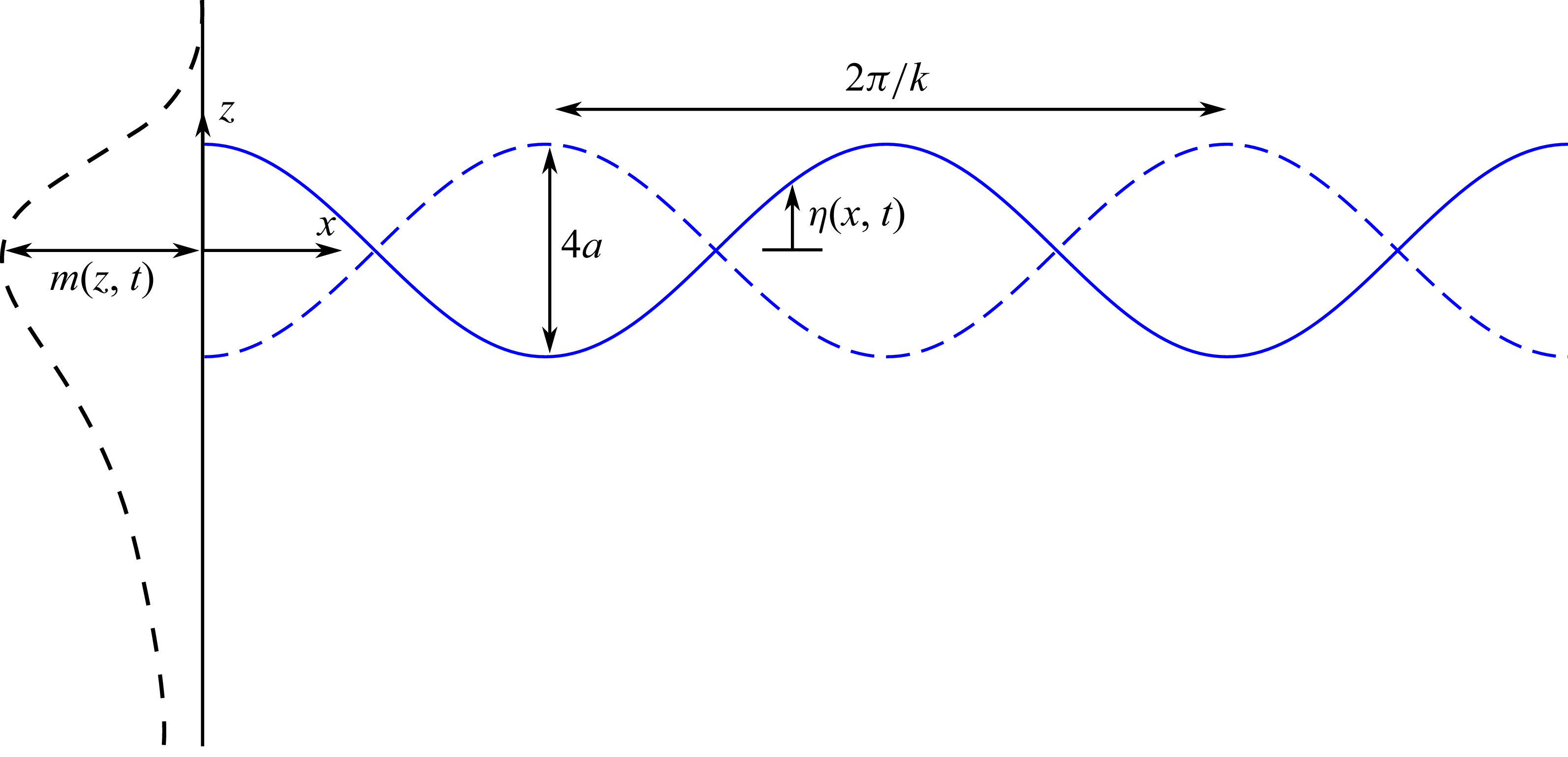


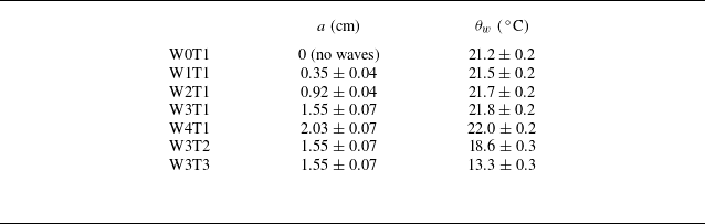


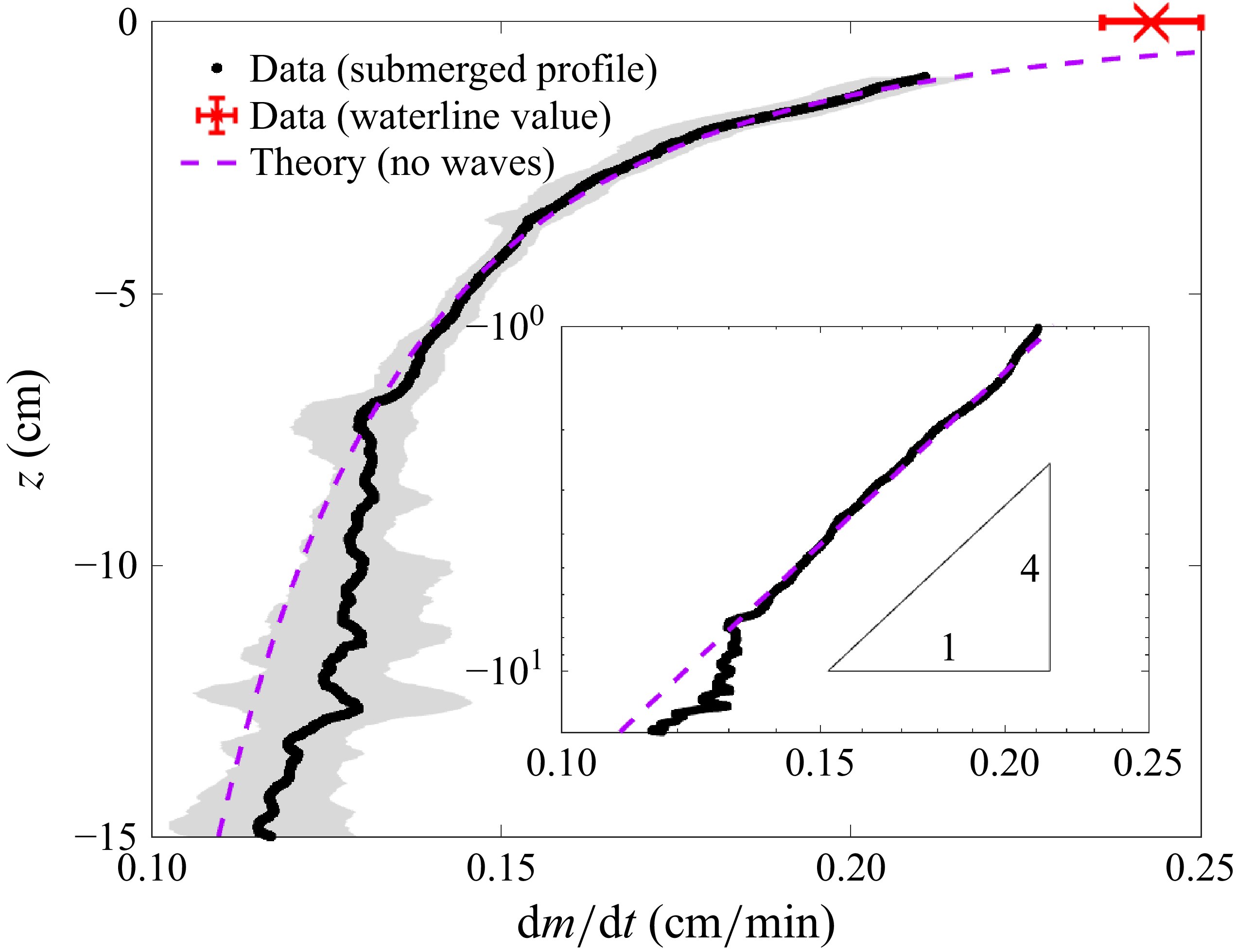


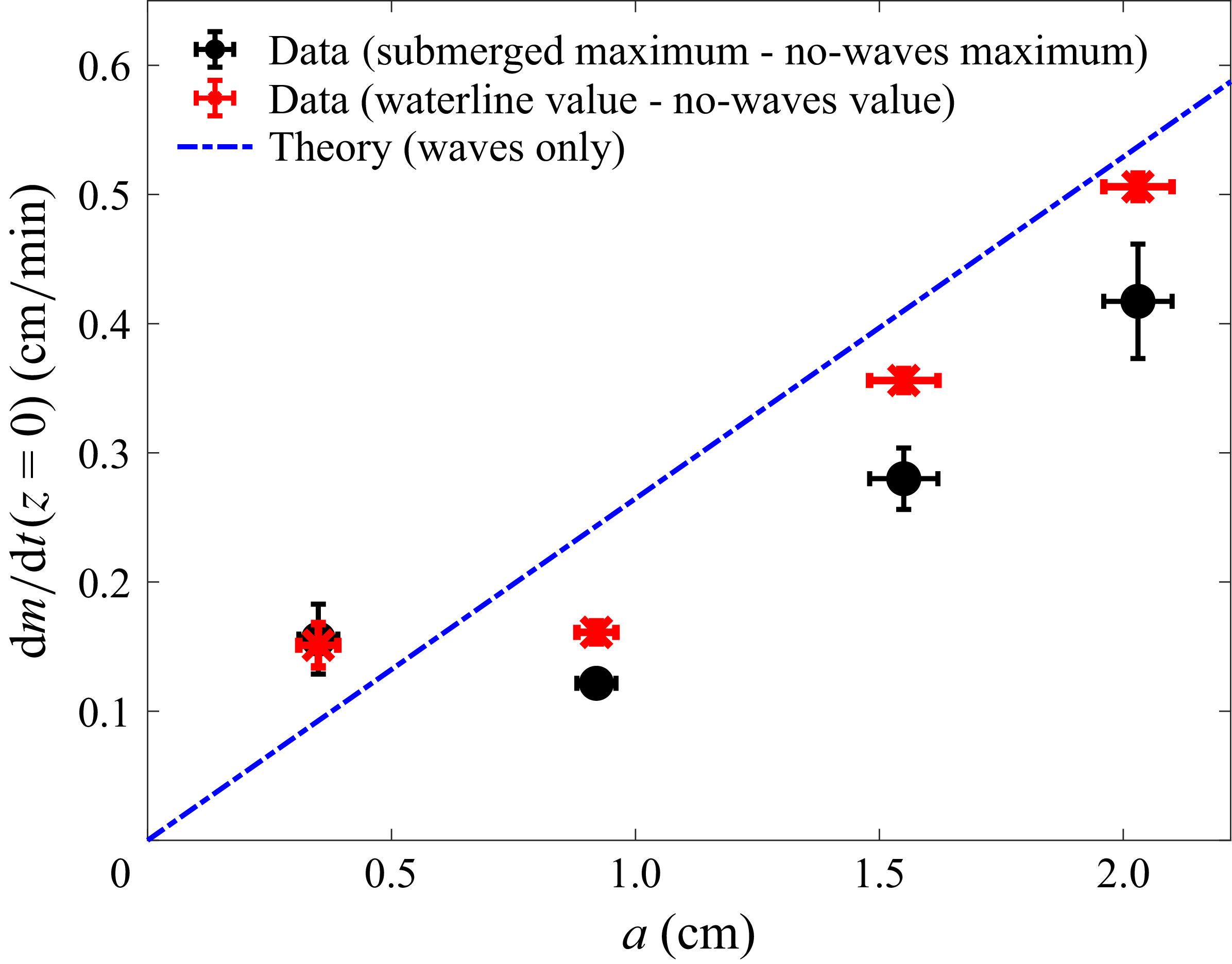


 Open access

