


1. Introduction
In reliability theory, one of the central challenges is to understand the behavior of those system components that remain functional after the overall system has failed at a specific time  $t$. Unlike conventional reliability metrics that emphasize inactivity periods or aggregate system lifetimes, our focus is directed toward the residual lifetimes of live components, which carry crucial information about the hidden resilience and structural dependencies of the system. To illustrate the practical implications of this viewpoint, we briefly mention two representative examples.
1—Consider a backup power system consisting of multiple battery cells arranged in a coherent structure. The system fails once a certain number of critical cells are exhausted; however, several other cells may remain alive at the system failure time. These live cells can be extracted and reused either for durability testing or in secondary applications. This approach not only reduces costs and resource waste but also provides valuable empirical data regarding the lifetime distribution of operational components.
2—Aircraft control systems are typically designed with redundancy. Even when the system as a whole is considered failed due to a critical fault, several sensors or controllers may still function properly. These live components can be recovered and subjected to stress testing. The results provide essential feedback for the development of safer control system architectures and for meeting rigorous certification requirements in the aerospace industry.
For clarity, we summarize below the main notations used throughout the paper. These symbols appear frequently in the derivation of conditional residual lifetimes, system signatures, and extropy-related measures. A complete table of notations is provided in Table 1.
Summary of notations used throughout the manuscript.

Table 1 Long description
The table is a notation glossary for a reliability and information-theory framework involving component lifetimes and coherent system lifetime. It defines the basic random lifetimes for multiple independent, identically distributed components and the ordered lifetimes used as order statistics. Several entries describe conditional and residual lifetimes, including conditioning on a time point falling between two ordered failures or between the system failure time and a specified ordered failure. It lists distribution-related functions for both components and the system, including cumulative distribution, density, survival, inverse distribution, and hazard rate. It also defines extropy-based quantities and divergences, including extropy, cumulative residual extropy, a Jensen-type divergence, and a relative measure comparing two variables. The remaining items define vectors and coefficients used for system characterization and design, such as the system signature, time-dependent conditional probability vector, mixing coefficient, design criterion, cost vector, information-weight vector, and an information cost index. Interpretations depend on the stated independence and identical distribution assumptions and on the specific conditioning events described for the conditional and residual lifetime terms.
For a coherent system of order  $n$ with lifetime $T(n)$, the signature of the system is represented by an $n$-dimensional probability vector $\boldsymbol s = (s_1,\ldots,s_n)$, where the $i$th element is defined as $s_{i} =P\big(T(n)=Y_{i:n}\big)$, and the condition $\sum_{i=1}^{n}s_i=1$ holds. The system signature describes how likely the system failure depends on the $i$th component failure. For example, a signature $(0.2,0.3,0.5)$ for a three-component system implies that the system most likely fails due to the third component. For further reading on system signature vectors, see [Reference Samaniego35].
In this paper, we analyze coherent systems whose signature vector takes the form
 \begin{equation*}
\boldsymbol s = (s_1,\ldots,s_i,0,\ldots,0), \qquad i = 1,\ldots,n-1.
\end{equation*}
\begin{equation*}
\boldsymbol s = (s_1,\ldots,s_i,0,\ldots,0), \qquad i = 1,\ldots,n-1.
\end{equation*} We assume that the system is initiated at time  $t = 0$. When the system has failed at time $t$, attention naturally shifts to those components that are observed to remain operational at the system failure instant, that is, components whose lifetimes satisfy $Y_i \gt T(n)=t$. In the conditional lifetime model used throughout this paper, the residual lifetime of such a live component is represented by
 \begin{equation*}
T_{j,n}(t) = Y_{j:n} - t \,\Big|\, T(n) \lt t \lt Y_{j:n},
\end{equation*}
\begin{equation*}
T_{j,n}(t) = Y_{j:n} - t \,\Big|\, T(n) \lt t \lt Y_{j:n},
\end{equation*}for  $t \gt 0$ and $j=i+1,\ldots,n$. This quantity captures the additional time that the $j$th order statistic can continue to operate beyond $t$, given that the overall system has already collapsed before $t$ but the component itself has survived until that moment. This formulation provides a rigorous probabilistic characterization of the residual lifetimes of components that outlive the system and thus plays a crucial role in reliability analysis. It allows engineers and system designers to quantify the potential reuse of these components in backup or secondary systems, to estimate how long they can be expected to function independently, and to assess how their presence influences resource allocation and maintenance strategies.
From [Reference Goliforushani, Asadi and Balakrishnan12], we have
 \begin{equation}
\bar{G}_{T_{j,n}(t)}(y) = \sum\limits_{k=1}^{i} p_k(t) \,\bar{G}_{Y_{j,k,n}(t)}(y),
\end{equation}
\begin{equation}
\bar{G}_{T_{j,n}(t)}(y) = \sum\limits_{k=1}^{i} p_k(t) \,\bar{G}_{Y_{j,k,n}(t)}(y),
\end{equation}where
 \begin{equation}
\bar{G}_{Y_{j,k,n}(t)}(y) = \sum\limits_{l=k}^{j-1} K_{l,j,k,n}(t)\,\bar{G}_{Y^t_{j-1:n-l}}(y),
\end{equation}
\begin{equation}
\bar{G}_{Y_{j,k,n}(t)}(y) = \sum\limits_{l=k}^{j-1} K_{l,j,k,n}(t)\,\bar{G}_{Y^t_{j-1:n-l}}(y),
\end{equation} \begin{equation}
\bar{G}_{Y^t_{j-1:n-l}}(y) = \sum\limits_{m=n-j+1}^{n-l}
\binom{n-l}{m}
\left( \frac{\bar{G}(y+t)}{\bar{G}(t)} \right)^{m}
\left( 1 - \frac{\bar{G}(y+t)}{\bar{G}(t)} \right)^{n-l-m},
\end{equation}
\begin{equation}
\bar{G}_{Y^t_{j-1:n-l}}(y) = \sum\limits_{m=n-j+1}^{n-l}
\binom{n-l}{m}
\left( \frac{\bar{G}(y+t)}{\bar{G}(t)} \right)^{m}
\left( 1 - \frac{\bar{G}(y+t)}{\bar{G}(t)} \right)^{n-l-m},
\end{equation} \begin{equation}
p_k(t) = \frac{s_k \big( \bar{G}_{Y_{j:n}}(t) - \bar{G}_{Y_{k:n}}(t) \big) }
{\sum\limits_{m=1}^{i} s_m \big( \bar{G}_{Y_{j:n}}(t) - \bar{G}_{Y_{m:n}}(t) \big) },
\end{equation}
\begin{equation}
p_k(t) = \frac{s_k \big( \bar{G}_{Y_{j:n}}(t) - \bar{G}_{Y_{k:n}}(t) \big) }
{\sum\limits_{m=1}^{i} s_m \big( \bar{G}_{Y_{j:n}}(t) - \bar{G}_{Y_{m:n}}(t) \big) },
\end{equation}and
 \begin{equation}
K_{l,j,k,n}(t) = \frac{\bar{G}_{Y_{l+1:n}}(t) - \bar{G}_{Y_{l:n}}(t) }
{\bar{G}_{Y_{j:n}}(t) - \bar{G}_{Y_{k:n}}(t)}.
\end{equation}
\begin{equation}
K_{l,j,k,n}(t) = \frac{\bar{G}_{Y_{l+1:n}}(t) - \bar{G}_{Y_{l:n}}(t) }
{\bar{G}_{Y_{j:n}}(t) - \bar{G}_{Y_{k:n}}(t)}.
\end{equation}Eqs. (1)–(5) follow from the conditional lifetime model introduced by [Reference Goliforushani, Asadi and Balakrishnan12]. The derivation of the corresponding SFs for this model is provided in Section 2 of their paper, to which the reader is referred for further details.
From an engineering perspective, the probability  $\bar{G}_{T_{j,n}(t)}(y)$ is a crucial tool for evaluating the performance of live components in failed systems. Intuitively, if a system has ceased operation but certain components are still functioning, $\bar{G}_{T_{j,n}(t)}(y)$ quantifies the likelihood that these components will remain alive for at least $y$ additional time units from the present moment, providing valuable insights for reuse decisions or maintenance planning.
Extensive studies have been devoted to the analysis of residual lifetimes of coherent systems across different frameworks; see, for example, [Reference Samaniego34], [Reference Kochar, Mukerjee and Samaniego18], [Reference Bairamov, Ahsanullah and Akhundov4], [Reference Khaledi and Shaked16], [Reference Asadi and Goliforushani3], [Reference Navarro and Hernandez22], [Reference Navarro, Balakrishnan and Samaniego21], [Reference Samaniego, Balakrishnan and Navarro36], [Reference Li and Lynch20], [Reference Zhang40], [Reference Zhang and Yang42], [Reference Gertsbakh, Shpungin and Spizzichino11], [Reference Balakrishnan and Asadi5], and [Reference Zhang41].
In the realm of information theory, entropy serves as a fundamental metric for quantifying the degree of uncertainty inherent in a random variable. Originally introduced by Shannon Shannon1948, this measure is mathematically expressed for a continuous random variable  $X$ with PDF $f(x)$ as
 \begin{equation*}
H(X) = -E\big(\log f(X)\big),
\end{equation*}
\begin{equation*}
H(X) = -E\big(\log f(X)\big),
\end{equation*}where “ $\log$” denotes the natural logarithm. Decades later, Lad et al. [Reference Lad, Sanfilippo and Agro19] proposed a complementary notion of uncertainty, termed extropy. Conceived as the dual counterpart of entropy, extropy has been characterized in the literature as capturing aspects such as structural order, vitality, energy, experiential richness, and the inherent tendency of systems toward growth and advancement. Formally, Lad et al. [Reference Lad, Sanfilippo and Agro19] defined the extropy of a non-negative random variable $X$ with PDF $f(x)$ by
 \begin{equation*}
J(X) = -\frac{1}{2}\int_{0}^{+\infty} f^2(x)\,dx
= -\frac{1}{2}\int_{0}^{1} f\big(F^{-1}(u)\big)\,du.
\end{equation*}
\begin{equation*}
J(X) = -\frac{1}{2}\int_{0}^{+\infty} f^2(x)\,dx
= -\frac{1}{2}\int_{0}^{1} f\big(F^{-1}(u)\big)\,du.
\end{equation*}A growing body of literature has investigated extropy and its applications in assessing the informational characteristics of reliability systems; see, for instance, [Reference Qiu28], [Reference Qiu and Jia29], [Reference Qiu and Jia30], [Reference Kayal15], [Reference Jose and Sathar14], [Reference Jahanshahi, Zarei and Khammar13], [Reference Pakdaman and Hashempour25], [Reference Chakraborty and Pradhan7], [Reference Chakraborty and Pradhan8], [Reference Chakraborty and Pradhan9], [Reference Chakraborty and Pradhan10], [Reference Pakdaman and Alizadeh Noughabi23], [Reference Pakdaman and Noughabi26], and [Reference Pakdaman and Alizadeh Noughabi24].
In coherent systems, the residual lifetimes of live components play a pivotal role in assessing system reliability and performance. As these systems become increasingly complex, with multiple interdependent failure modes, conventional reliability metrics such as failure rates or mean time to failure often fail to provide a complete picture of system behavior. Consequently, cumulative residual measures such as the CRJ offer a powerful framework for analyzing the residual structure and interdependencies among components Shannon1948,JahanshahiZareiKhammar2020, Shannon1948,JahanshahiZareiKhammar2020. Cumulative residual entropy was initially introduced by Rao et al. [Reference Rao, Chen, Vemuri and Wang32] based on the SF of  $X$. Later, Jahanshahi et al. [Reference Jahanshahi, Zarei and Khammar13] proposed the CRJ, defined as
 \begin{equation}
\xi J\big( X \big) = -\frac{1}{2}\int_0^\infty \bar F^2(x)\,dx.
\end{equation}
\begin{equation}
\xi J\big( X \big) = -\frac{1}{2}\int_0^\infty \bar F^2(x)\,dx.
\end{equation}Despite significant progress in uncertainty quantification for reliability systems, most entropy- and extropy-based measures treat lifetimes in an unconditional manner and therefore fail to capture the structural changes induced by conditioning on system failure and component survival. As a consequence, two coherent systems may appear similar under global performance metrics, while their conditional residual behaviors after failure differ substantially.
• Formal gap: Existing uncertainty indices (such as Shannon entropy, cumulative residual entropy, and classical extropy) do not directly target the conditional lifetimes of live components and have rarely been developed in the setting of the Goliforushani model.
• Limitations of prior metrics: Classical entropy-type indices are largely insensitive to the diversity of conditional residual distributions and do not incorporate the structural role of the system signature.
• What this paper provides: A unified framework of comparison results, bounds, and design principles for CRJ and its JCRJ divergence, tailored to the lifetimes of live components.
• Impact on system design: The proposed measures separate system architectures that appear identical under unconditional metrics, rank them by conditional uncertainty, and guide the selection of signature vectors that balance information-theoretic performance with cost and structural complexity.
In this framework, CRJ serves as a primary metric of uncertainty in the conditional residual lifetimes of live components, while JCRJ refines this perspective by quantifying divergence between conditional residual distributions. Embedding these measures into the signature representation of coherent systems links the informational content of post-failure survival directly to system architecture and enables their use in structural comparison and design. This paper develops a systematic treatment of CRJ and JCRJ for the residual lifetimes of live components in coherent systems. The main contributions are:
• Derivation of explicit representations of the CRJ of $T_{j,n}(t)$ in terms of system signatures and conditional mixing coefficients, together with stochastic comparison results and theoretical bounds.
• Introduction and analysis of the JCRJ divergence for comparing conditional residual lifetime distributions, demonstrating its discriminating power relative to classical entropy-based measures.
• Application of the CRJ/JCRJ framework to systems with gamma lifetimes and exponentiated Weibull (EW) lifetimes exhibiting bathtub-shaped hazards, showing how heavy tails and non-monotone hazard rates affect conditional uncertainty.
• Formulation of an information-theoretic design criterion for optimal signature selection, balancing JCRJ-based uncertainty, cost, and structural complexity, with optimal signatures computed for several parametric settings.

This work investigates the CRJ associated with the residual lifetimes of live components in a coherent system, specifically focusing on scenarios where certain components remain operational at the system’s failure time  $t$, as formalized in Eq. (1). The paper is organized as follows. Section 2 presents a comprehensive formulation of the CRJ for the residual lifetimes of live components, leveraging the conditional coefficient vector, and develops corresponding stochastic comparisons and theoretical bounds. Section 3 introduces a divergence measure designed to quantify the complexity inherent in the residual lifetimes of alive components. In Section 4, the CRJ and JCRJ frameworks are applied to a gamma-distributed system comprising four IID components, allowing an examination of residual lifetimes across multiple system configurations. Section 5 addresses the identification of an optimal signature vector that simultaneously minimizes the JCRJ divergence and associated costs, providing a principled approach for system optimization. Finally, Section 6 offers concluding insights and synthesizes the principal findings of the study, highlighting both theoretical contributions and practical implications.
2. CRJ of residual lifetimes of live components
Let  $Y_1, \ldots, Y_n$ represent the lifetimes of IID components, with the CDF $G$ for a coherent system of order n characterized by the signature vector $\pmb s = (s_1, \ldots , s_i, 0, \ldots, 0)$, $i = 1, \ldots , n-1$. The goal is to compute the CRJ of the residual lifetimes of live components, or equivalently, the CRJ of $Y_{j:n}-t|T(n) \lt t \lt Y_{j:n}$. In this section, we derive an expression for the CRJ of the residual lifetimes of live components, given the signature vector $\pmb s = (s_1, \ldots , s_i, 0, \ldots, 0)$ for $i = 1, \ldots,n-1$. Using Eqs. (1) and (6), the CRJ for $T_{j,n}(t)$ is expressed as
 \begin{align}
\xi J\left( T_{j,n}(t) \right) &= - \frac{1}{2}\int_0^\infty \bar{G}^2_{T_{j,n}(t)}(y)~dy\nonumber\\
&= - \frac{1}{2}\int_0^\infty \Big(\sum\limits_{k=1}^{i} p_k(t) \bar{G}_{Y_{j,k,n}(t)}(y)\Big)^2~dy
\nonumber\\
&= - \frac{1}{2}\int_0^\infty\Big(\sum\limits_{k=1}^{i}\sum\limits_{l=k}^{j-1} p_k(t) K_{l,j,k,n}(t)\,\bar{G}_{Y^t_{j-1:n-l}}(y)\Big)^2~dy
\nonumber\\
&= - \frac{1}{2}\int_0^\infty\Big(1-\sum\limits_{k=1}^{i}\sum\limits_{l=k}^{j-1} p_k(t) K_{l,j,k,n}(t)(j-l)\binom{n-l}{n-j}\nonumber\\
&\quad \times \int_{\frac{\bar{G}(y+t)}{\bar{G}(t)}}^{1}u^{n-j}(1-u)^{j-l-1}~du\Big)^2~dy.\end{align}
\begin{align}
\xi J\left( T_{j,n}(t) \right) &= - \frac{1}{2}\int_0^\infty \bar{G}^2_{T_{j,n}(t)}(y)~dy\nonumber\\
&= - \frac{1}{2}\int_0^\infty \Big(\sum\limits_{k=1}^{i} p_k(t) \bar{G}_{Y_{j,k,n}(t)}(y)\Big)^2~dy
\nonumber\\
&= - \frac{1}{2}\int_0^\infty\Big(\sum\limits_{k=1}^{i}\sum\limits_{l=k}^{j-1} p_k(t) K_{l,j,k,n}(t)\,\bar{G}_{Y^t_{j-1:n-l}}(y)\Big)^2~dy
\nonumber\\
&= - \frac{1}{2}\int_0^\infty\Big(1-\sum\limits_{k=1}^{i}\sum\limits_{l=k}^{j-1} p_k(t) K_{l,j,k,n}(t)(j-l)\binom{n-l}{n-j}\nonumber\\
&\quad \times \int_{\frac{\bar{G}(y+t)}{\bar{G}(t)}}^{1}u^{n-j}(1-u)^{j-l-1}~du\Big)^2~dy.\end{align}The last inequality of Eq. (7) follows directly from the relation below
 \begin{align}
\bar{G}_{Y^t_{j-1:n-l}}(y) &= \sum\limits_{m=n-j+1}^{n-l}
\binom{n-l}{m}
\left( \frac{\bar{G}(y+t)}{\bar{G}(t)} \right)^{m}
\left( 1 - \frac{\bar{G}(y+t)}{\bar{G}(t)} \right)^{n-l-m}\nonumber\\
&= 1-\sum\limits_{m=0}^{n-j}
\binom{n-l}{m}
\left( \frac{\bar{G}(y+t)}{\bar{G}(t)} \right)^{m}
\left( 1 - \frac{\bar{G}(y+t)}{\bar{G}(t)} \right)^{n-l-m}\nonumber\\
&= 1-(j-l)\binom{n-l}{n-j}\int_{\frac{\bar{G}(y+t)}{\bar{G}(t)}}^{1}u^{n-j}(1-u)^{j-l-1}~du.
\end{align}
\begin{align}
\bar{G}_{Y^t_{j-1:n-l}}(y) &= \sum\limits_{m=n-j+1}^{n-l}
\binom{n-l}{m}
\left( \frac{\bar{G}(y+t)}{\bar{G}(t)} \right)^{m}
\left( 1 - \frac{\bar{G}(y+t)}{\bar{G}(t)} \right)^{n-l-m}\nonumber\\
&= 1-\sum\limits_{m=0}^{n-j}
\binom{n-l}{m}
\left( \frac{\bar{G}(y+t)}{\bar{G}(t)} \right)^{m}
\left( 1 - \frac{\bar{G}(y+t)}{\bar{G}(t)} \right)^{n-l-m}\nonumber\\
&= 1-(j-l)\binom{n-l}{n-j}\int_{\frac{\bar{G}(y+t)}{\bar{G}(t)}}^{1}u^{n-j}(1-u)^{j-l-1}~du.
\end{align}For further details and a comprehensive discussion of this construction, the reader is referred to Lemma 2 in [Reference Goliforushani, Asadi and Balakrishnan12].
In what follows, we aim to derive a more tractable representation for the CRJ of the residual lifetimes of live components. Initially, several inner components of Eq. (7) are simplified, after which a more compact form of the equation as a whole is obtained. To begin with, we start by considering the product of the two terms  $p_k(t)$ and $K_{l,j,k,n}(t)$, which can be simplified as follows:
 \begin{equation}
p_k(t) K_{l,j,k,n}(t)=\frac{s_k\binom{n}{l} G^l(t)\bar{G}^{n-l}(t)}{\sum\limits_{m=1}^{i} s_m \big( \bar{G}_{Y_{j:n}}(t) - \bar{G}_{Y_{m:n}}(t) \big)}.
\end{equation}
\begin{equation}
p_k(t) K_{l,j,k,n}(t)=\frac{s_k\binom{n}{l} G^l(t)\bar{G}^{n-l}(t)}{\sum\limits_{m=1}^{i} s_m \big( \bar{G}_{Y_{j:n}}(t) - \bar{G}_{Y_{m:n}}(t) \big)}.
\end{equation} By taking into account the identity  $\sum\limits_{k=1}^{i}\sum\limits_{l=k}^{j-1} p_k(t) K_{l,j,k,n}(t)=1$ and performing the substitution of Eq. (9) into Eq. (7), we immediately arrive at the following simplified representation:
 \begin{align}
\xi J\left( T_{j,n}(t) \right) &= - \frac{1}{2}\int_0^\infty\Big(1-\frac{\bar{G}^{n}(t)}{\sum\limits_{m=1}^{i} s_m \big( \bar{G}_{Y_{j:n}}(t) - \bar{G}_{Y_{m:n}}(t) \big)}\sum\limits_{k=1}^{i}s_k\sum\limits_{l=k}^{j-1} (j-l)\binom{n-l}{n-j}\binom{n}{l}(\frac{G(t)}{\bar{G}(t)})^l\nonumber\\
&\quad \times \int_{\frac{\bar{G}(y+t)}{\bar{G}(t)}}^{1}u^{n-j}(1-u)^{j-l-1}~du\Big)^2~dy.\end{align}
\begin{align}
\xi J\left( T_{j,n}(t) \right) &= - \frac{1}{2}\int_0^\infty\Big(1-\frac{\bar{G}^{n}(t)}{\sum\limits_{m=1}^{i} s_m \big( \bar{G}_{Y_{j:n}}(t) - \bar{G}_{Y_{m:n}}(t) \big)}\sum\limits_{k=1}^{i}s_k\sum\limits_{l=k}^{j-1} (j-l)\binom{n-l}{n-j}\binom{n}{l}(\frac{G(t)}{\bar{G}(t)})^l\nonumber\\
&\quad \times \int_{\frac{\bar{G}(y+t)}{\bar{G}(t)}}^{1}u^{n-j}(1-u)^{j-l-1}~du\Big)^2~dy.\end{align} Eq. (7) introduces a systematic approach for comparing the CRJ corresponding to two residual lifetimes of live components, where the comparison is governed by the coefficient vector  $\pmb p(t) = (p_1(t), \ldots , p_i(t), 0,\ldots , 0)$. This vector can be viewed as the conditional signature of the system, encapsulating the probabilistic influence of individual components on system failure under a specific conditioning framework. In particular, each element $p_k(t)$ measures the probability that the component with lifetime $X_{k:n}$ is the one responsible for triggering the failure, given that the system has already failed but all components with lifetimes $X_{k:n}$, $k = i + 1, i + 2, \ldots , n$, remain operational at time $t$. Such an interpretation provides engineers and reliability theorists with deeper insight into the structural behavior of the system. It not only quantifies the role of specific components in driving the failure but also highlights how the survival of higher-ordered components affects system reliability. Consequently, the conditional signature serves as a powerful analytical tool, allowing for a more refined assessment of system vulnerability and guiding the design of systems where failure attribution and conditional reliability play a critical role. Next, we present an example that demonstrates how the CRJ can be computed by employing Eq. (10).
Example 1. Consider a coherent system characterized by the signature vector  $\pmb s =(\frac{1}{4},\frac{5}{12},\frac{1}{3},0)$, which consists of four IID components. Each component lifetime follows a Gamma distribution with PDF $g(y) = 4ye^{-2y},~y \gt 0$, and the CDF $G(y) = 1 - (1 + 2y)e^{-2y}$. According to the structure induced by the signature, the system lifetime is given by $T(4) = \min(Y_2, \max(Y_1, Y_3))$. The fourth component is irrelevant in the sense of coherent system theory; that is, the system’s state does not change when the state of this component changes. This is reflected by its zero signature weight, and consequently, it does not appear in the expression for $T(4)$.
By applying Eq. (10), we derive the CRJ associated with the residual lifetimes of the live components of the system for  $j=4$ as follows
 \begin{align*}
\xi J\left( T_{4,4}(t) \right)=- \frac{1}{2}\int_0^\infty\Big(1-\frac{\bar{G}^{3}(t)}{G(t)\Big(\bar{G}^{2}(t)+4G(t)\Big)}\sum\limits_{k=1}^{3}s_k\sum\limits_{l=k}^{3} \binom{4}{l}(\frac{G(t)}{\bar{G}(t)})^l(1-\frac{\bar{G}(y+t)}{\bar{G}(t)})^{4-l}\Big)^2~dy.\nonumber\\
\end{align*}
\begin{align*}
\xi J\left( T_{4,4}(t) \right)=- \frac{1}{2}\int_0^\infty\Big(1-\frac{\bar{G}^{3}(t)}{G(t)\Big(\bar{G}^{2}(t)+4G(t)\Big)}\sum\limits_{k=1}^{3}s_k\sum\limits_{l=k}^{3} \binom{4}{l}(\frac{G(t)}{\bar{G}(t)})^l(1-\frac{\bar{G}(y+t)}{\bar{G}(t)})^{4-l}\Big)^2~dy.\nonumber\\
\end{align*} The plotted curve in Figure 1 represents the CRJ of the residual lifetimes of the live components in the coherent system  $T(4) = \min(Y_2, \max(Y_1, Y_3))$. The curve is increasing with $t$, which intuitively shows that as time progresses, the system’s residual lifetimes of the live components become more certain. Smaller CRJ values correspond to higher uncertainty, while larger CRJ values indicate lower uncertainty.
CRJ values  $\xi J\left( T_{4,4}(t)\right)$ of the residual lifetimes of the live components of system with lifetime $T(4) = \min(Y_2, \max(Y_1, Y_3))$ in Example 1.

Figure 1 Long description
The x-axis label is t. The x-axis ranges from 0 to 100, with tick labels at 0, 20, 40, 60, 80 and 100. The y-axis label is xi J of T subscript 4 comma 4 of t. The y-axis ranges from 0.0 to minus 0.7, with tick labels at 0.0, minus 0.1, minus 0.2, minus 0.3, minus 0.4, minus 0.5, minus 0.6 and minus 0.7. One dashed curve starts near t equals 0 at about minus 0.6, rises steeply to about minus 0.2, then continues rising more gradually and becomes nearly flat near minus 0.13 by about t equals 10, remaining close to that level through t equals 100. One dotted horizontal line is drawn near minus 0.13 across the plot area. A numeric label near the right side reads minus 0.125625.
Since the CRJ measure is always negative, an increase in its value means that the curve moves upward toward zero. Therefore, in Figure 1, the statement that the CRJ increases with  $t$ should be interpreted as “the CRJ increases toward zero as $t$ grows,” which reflects a decrease in the system’s uncertainty.
The red dashed line represents the convergence value of CRJ, which in this case is approximately  $-$0.125, meaning that after a long time, the system reaches a stable level of certainty for the residual lifetimes of the live components.
To further illustrate the behavior of the CRJ measure beyond classical lifetime models, we now consider a case in which the component lifetimes follow a distribution with a bathtub-shaped hazard rate. Such models are commonly used in reliability engineering to capture early failures, a stable operating period, and wear-out phenomena.
Example 2. Consider a coherent system characterized by the signature vector  $
\pmb{s}=\left(\tfrac14,\,\tfrac{5}{12},\,\tfrac13,\,0\right),
$ consisting of four IID components. In this example, each component lifetime follows an EW distribution with CDF
$
\pmb{s}=\left(\tfrac14,\,\tfrac{5}{12},\,\tfrac13,\,0\right),
$ consisting of four IID components. In this example, each component lifetime follows an EW distribution with CDF  $
G(y)=\left(1-e^{-(y/\lambda)^{\beta}}\right)^{\alpha}, ~ y \gt 0,
$ and PDF
$
G(y)=\left(1-e^{-(y/\lambda)^{\beta}}\right)^{\alpha}, ~ y \gt 0,
$ and PDF  $
g(y)=\alpha\,\beta\,\lambda^{-\beta}\,y^{\beta-1}
e^{-(y/\lambda)^{\beta}}
\left(1-e^{-(y/\lambda)^{\beta}}\right)^{\alpha-1}, ~ y \gt 0,
$ where
$
g(y)=\alpha\,\beta\,\lambda^{-\beta}\,y^{\beta-1}
e^{-(y/\lambda)^{\beta}}
\left(1-e^{-(y/\lambda)^{\beta}}\right)^{\alpha-1}, ~ y \gt 0,
$ where  $\alpha \gt 0$, $\beta \gt 0$, and $\lambda \gt 0$ are shape and scale parameters. This family is highly flexible and can generate various hazard-rate patterns, including bathtub-shaped hazards, which are frequently encountered in reliability engineering. According to the structure induced by the system signature, the system lifetime is
  $
T(4)=\min\big(Y_2,\,\max(Y_1,Y_3)\big).
$ In the numerical study below, four sets of EW parameters that produce bathtub-shaped hazards are considered:
$
T(4)=\min\big(Y_2,\,\max(Y_1,Y_3)\big).
$ In the numerical study below, four sets of EW parameters that produce bathtub-shaped hazards are considered:
 \begin{equation*}
(\alpha,\beta,\lambda)\in
\{(0.4,1.5,1),\; (0.4,1.5,2),\; (0.5,1.5,1),\; (0.5,1.5,2)\}.
\end{equation*}
\begin{equation*}
(\alpha,\beta,\lambda)\in
\{(0.4,1.5,1),\; (0.4,1.5,2),\; (0.5,1.5,1),\; (0.5,1.5,2)\}.
\end{equation*} The plotted curves in Figure 2 exhibit the typical bathtub-shaped pattern: an initially high hazard (early failures), a decreasing region approaching a nearly flat regime (useful life), and a final increasing phase (wear-out). Increasing  $\lambda$ stretches the distribution, delaying the transitions between phases, while larger $\alpha$ produces smoother and more stable middle regions.
Hazard-rate functions of the EW distribution for the four parameter sets  $(\alpha,\beta,\lambda)\in \{(0.4,1.5,1),\,(0.4,1.5,2),\,(0.5,1.5,1),\,(0.5,1.5,2)\}$, showing clear bathtub-shaped behavior.

Figure 2 Long description
The y-axis label is h(t). The x-axis label is t. The x-axis ranges from 0 to 5 with labeled ticks at 0, 1, 2, 3, 4 and 5. The y-axis ranges from 0 to 10 with labeled ticks at 0, 2, 4, 6, 8 and 10. A legend lists four series: alpha equals 0.4, beta equals 1.5, lambda equals 1; alpha equals 0.4, beta equals 1.5, lambda equals 2; alpha equals 0.5, beta equals 1.5, lambda equals 1; alpha equals 0.5, beta equals 1.5, lambda equals 2. All four curves start at high values near t equals 0, drop steeply, then increase gradually from about t equals 1 to t equals 5. For the series alpha equals 0.4, beta equals 1.5, lambda equals 1, plotted markers are shown at t equals 1, 2, 3, 4 and 5 with h(t) values about 1.7, 2.1, 2.6, 3.0 and 3.3. For the series alpha equals 0.5, beta equals 1.5, lambda equals 1, plotted markers are shown at t equals 1, 2, 3, 4 and 5 with h(t) values about 1.6, 2.1, 2.6, 3.0 and 3.3. For the series alpha equals 0.4, beta equals 1.5, lambda equals 2, plotted markers are shown at t equals 1, 2, 3, 4 and 5 with h(t) values about 0.8, 0.9, 1.0, 1.1 and 1.2. For the series alpha equals 0.5, beta equals 1.5, lambda equals 2, plotted markers are shown at t equals 1, 2, 3, 4 and 5 with h(t) values about 0.7, 0.8, 0.9, 1.0 and 1.1.
Figure 3 displays the behavior of  $\xi J(T_{4,4}(t))$. All curves increase with $t$ and move upward toward zero, indicating that the residual lifetimes of the live components become more certain as time progresses. Since CRJ is always negative, larger (less negative) values indicate lower uncertainty. A detailed comparison of the four curves reveals meaningful differences. The ordering of the CRJ curves in Figure 3 can be interpreted in light of the bathtub-shaped hazard rate of the EW distribution. For this family, the scale parameter $\lambda$ stretches the time axis: larger values of $\lambda$ keep the system longer in the early and middle phases of the bathtub, where the conditional residual lifetimes of the live components are more dispersed. This increased dispersion of the residual lifetimes translates into more negative values of the CRJ functional, that is, higher uncertainty.
CRJ values  $\xi J(T_{4,4}(t))$ of the residual lifetimes of the live components under the four EW parameter sets in Example 2.

Figure 3 Long description
Xi J(T subscript 4 comma 4 (t)) The horizontal axis is labeled t, ranging from 0 to 30 with labeled ticks at 0, 5, 10, 15, 20, 25 and 30. The vertical axis is labeled xi J(T subscript 4 comma 4 (t)), ranging from minus 1.0 to 0.0 with labeled ticks at 0.0, minus 0.2, minus 0.4, minus 0.6, minus 0.8 and minus 1.0. A legend lists four series: alpha equals 0.4, beta equals 1.5, lambda equals 1; alpha equals 0.4, beta equals 1.5, lambda equals 2; alpha equals 0.5, beta equals 1.5, lambda equals 1; alpha equals 0.5, beta equals 1.5, lambda equals 2. The series alpha equals 0.4, beta equals 1.5, lambda equals 1 starts near t equals 0 at about minus 0.35 and increases to about minus 0.12 by around t equals 3. It continues increasing and reaches 0.0 at about t equals 12, then stays at 0.0 from about t equals 12 to t equals 30. The series alpha equals 0.4, beta equals 1.5, lambda equals 2 starts near t equals 0 at about minus 0.65 and increases to about minus 0.28 by around t equals 3. It continues increasing gradually to about minus 0.12 by around t equals 20, then rises to 0.0 at about t equals 23 and stays at 0.0 from about t equals 23 to t equals 30. The series alpha equals 0.5, beta equals 1.5, lambda equals 1 starts near t equals 0 at about minus 0.40 and increases to about minus 0.12 by around t equals 3. It continues increasing and reaches 0.0 at about t equals 12, then stays at 0.0 from about t equals 12 to t equals 30. The series alpha equals 0.5, beta equals 1.5, lambda equals 2 starts near t equals 0 at about minus 0.75 and increases to about minus 0.28 by around t equals 3. It continues increasing gradually to about minus 0.13 by around t equals 21, then rises to 0.0 at about t equals 23 and stays at 0.0 from about t equals 23 to t equals 30.
Similarly, the exponentiation parameter  $\alpha$ redistributes probability mass between the early- and late-failure regions. In the parameter region considered here ( $\alpha \in \{0.4,0.5\}$ and $\beta=1.5$), increasing $\alpha$ strengthens the bathtub behavior and produces heavier tails, which again results in a more spread-out distribution of the residual lifetimes and therefore smaller (more negative) CRJ values.
Consequently, the parameter set  $(\alpha,\lambda)=(0.4,1)$ yields the largest (least negative) CRJ values and thus the lowest uncertainty, followed by $(0.5,1)$, $(0.4,2)$, and finally $(0.5,2)$, which produces the smallest (most negative) CRJ values and the highest uncertainty among the four cases.
Overall, these results demonstrate that the CRJ measure effectively captures how the structural uncertainty of the live components is influenced by the parameters of the EW distribution, particularly in settings involving bathtub-shaped hazard functions.
Example 3. Consider a coherent system characterized by the signature vector  $\pmb s =(1,0,\ldots,0)$, which consists of $n$ IID components. Each component lifetime follows a Gamma distribution with PDF $g(y) = 4ye^{-2y},~y \gt 0$, and the CDF $G(y) = 1 - (1 + 2y)e^{-2y}$. According to the structure induced by the signature, the system lifetime is given by $T(n) = \min(Y_1, \ldots,Y_n)$. In the present example, the system is a series system, so the system fails as soon as the earliest component fails. At the instant of interest, we consider a live component indexed by the order statistic $Y_{j:n}$ (with $j=i+1,\ldots,n$; for the series case $i=1$ and the live component indices are $2,\dots,n$). In other words, at that moment, all remaining components with lifetimes $Y_{2:n}, Y_{3:n}, \dots, Y_{n:n}$ are still operational. The conditional residual lifetime of that component observed at epoch $t \gt 0$ is written as $Y_{j:n }- t \mid T(n) \lt t \lt Y_{j:n}$ for $j=2,\ldots,n$. In this example, we consider $j=3$. When $j=3$, the residual lifetime of interest is $Y_{3:n }- t \mid T(n) \lt t \lt Y_{3:n}$, that is, the additional time that the third-order component continues to operate after the system has failed, conditional on it being alive at observation time $t$. In what follows, by applying Eq. (10), we proceed to derive the CRJ associated with $Y_{3:n }- t|T(n) \lt t \lt Y_{3:n}$.
 \begin{align*}
\xi J\left( T_{3,n}(t) \right)&= - \frac{1}{2}\int_0^\infty \Bigg(
1-\frac{2\bar{G}(t)}{n(n-4)(2+(n-3)G(t))}\nonumber\\ &\times \Big[3(n-2)(\frac{\bar{G}(y+t)}{\bar{G}(t)})^{n-4}(\frac{1}{n-4}-\frac{1}{n-1}(\frac{\bar{G}(y+t)}{\bar{G}(t)})^{3})\nonumber\\ &+ \frac{n(n-1)G(t)}{2\bar{G}(t)}(1-(\frac{\bar{G}(y+t)}{\bar{G}(t)})^{4})\Big]\Bigg)^2~dy.
\end{align*}
\begin{align*}
\xi J\left( T_{3,n}(t) \right)&= - \frac{1}{2}\int_0^\infty \Bigg(
1-\frac{2\bar{G}(t)}{n(n-4)(2+(n-3)G(t))}\nonumber\\ &\times \Big[3(n-2)(\frac{\bar{G}(y+t)}{\bar{G}(t)})^{n-4}(\frac{1}{n-4}-\frac{1}{n-1}(\frac{\bar{G}(y+t)}{\bar{G}(t)})^{3})\nonumber\\ &+ \frac{n(n-1)G(t)}{2\bar{G}(t)}(1-(\frac{\bar{G}(y+t)}{\bar{G}(t)})^{4})\Big]\Bigg)^2~dy.
\end{align*} Figure 4 illustrates the behavior of the CRJ as a function of time  $t$ for different system sizes $n = 5, 6, 7, 8$. The convergence of each curve indicates that the uncertainty of the system stabilizes at long lifetimes, meaning that the measure captures the asymptotic behavior of the remaining components. When comparing across different values of $n$, it is observed that as $n$ increases, the CRJ values decrease (become more negative). This aligns with the interpretation that a smaller CRJ indicates a higher degree of uncertainty in the residual lifetimes. Larger systems (greater $n$) inherently have more components still alive after system failure, making the joint survival structure more complex and thereby spreading the probability mass more thinly across possible lifetimes. Consequently, the system’s CRJ is smaller, reflecting greater uncertainty in the residual lifetime distribution as the system size grows. The CRJ plot illustrates that as time progresses, the amount of “residual information” or uncertainty about the system’s remaining lifetime converges to a constant value. As the number of components $n$ increases, the CRJ decreases, in other words, larger systems exhibit greater uncertainty regarding the residual lifetimes of their components. The reason is that with more components, after the system fails, a larger number of components remain alive, making the residual lifetime more variable and dispersed. Therefore, the plot indicates that larger systems carry higher risk and uncertainty in terms of component survival after system failure.
Behavior of the CRJ  $\xi J\left( T_{3,n}(t)\right)$ as a function of $t$ for different system sizes ( $n = 5, 6, 7, 8$). The plot shows that CRJ decreases as the number of components increases, reflecting higher uncertainty in the residual lifetimes of larger systems.

Figure 4 Long description
The horizontal axis label is t. The horizontal axis range is 0 to 50. The vertical axis label is xi J( T subscript 3 comma n (t)). The vertical axis range is minus 0.05 to minus 0.025. Legend entries and line styles: n equals 8 is a solid line. n equals 7 is a dashed line. n equals 6 is a dotted line. n equals 5 is a dash dot line. Numeric labels printed near the curves: n equals 5 has minus 0.021042. n equals 6 has minus 0.025251. n equals 7 has minus 0.031563. n equals 8 has minus 0.042084. All four curves rise quickly from near t equals 0 and then flatten toward the printed numeric levels as t increases. The n equals 8 curve stays at the lowest level among the four and the n equals 5 curve stays at the highest level among the four.
By employing Eq. (7), the CRJ index corresponding to two residual lifetimes of live components can be systematically assessed, thereby enabling a comparative analysis across different systems. As a preliminary step, it is useful to recall the notions of several stochastic orderings, which provide the theoretical foundation for such comparisons. These concepts have been extensively discussed in the literature, particularly in the works of Shaked and Shanthikumar [Reference Shaked and Shanthikumar38] as well as Belzunce et al. [Reference Belzunce, Riquelme and Mulero6].
Definition. (Stochastic orders) Let  $X$ and $Y$ be two random variables with CDFs $F$ and $G$ and PDFs $f$ and $g$, respectively. Then $X$ is said to be smaller than $Y$ in the sense of:
(i) usual stochastic order (denoted by
$X\leqslant_{st}Y$ or
$F\leqslant_{st}G$) if
$ \bar{F}(x)\leq \bar{G}(x)$ for all
$x$;(ii) hazard rate order (denoted by
$X\leqslant_{hr}Y$ or
$F\leqslant_{hr}G$) if
${\displaystyle \frac{\bar{G}(x)}{\bar{F}(x)}}$ is increasing in
$x$.(iii) disperse order (denoted by
$X\leqslant_{disp}Y$ or
$F\leqslant_{disp}G$) if
$g(G^{-1}(v))\leq f(F^{-1}(v))$ for all
$0 \lt v \lt 1$. Also, let
$\boldsymbol{p}$ and
$\boldsymbol{q}$ be two discrete distributions on the integers
$\{1, ..., n\}$. Then, it is said that (see, e.g., [Reference Kochar, Mukerjee and Samaniego18]).(iv)
$\boldsymbol{p}\leqslant _{st}\boldsymbol{q}$ if and only if
$\sum\limits_{i=j}^{n}p_{i}\leq \sum\limits_{i=j}^{n}q_{i}$, for
$j=1,\ldots,n$.(v)
$\textbf{p}\leqslant _{hr}\textbf{q}$ if and only if
${\sum\limits_{i=j}^{n}p_{i}}\Big/{\sum\limits_{i=j}^{n}q_{i}}$ is decreasing in
$j$, for
$j=1,\ldots,n$.(vi)
$\textbf{p}\leqslant _{lr}\textbf{q}$ if and only if
${p_{i}}/q_{i}$ is decreasing in
$i$, for
$i=1,\ldots,n$ when
$p_{i},q_{i} \gt 0$.


In the subsequent analysis, let us define the model function of the system as
 \begin{equation*}{\cal{M}}_{T_{j,n}(t), Y_{j,k,n}(t), Y^t_{j-1-:n-l},\boldsymbol{p}(t),Y,G}=\{T_{j,n}(t), Y_{j,k,n}(t), Y^t_{j-1-:n-l},\boldsymbol{p}(t),Y,G \},
\end{equation*}
\begin{equation*}{\cal{M}}_{T_{j,n}(t), Y_{j,k,n}(t), Y^t_{j-1-:n-l},\boldsymbol{p}(t),Y,G}=\{T_{j,n}(t), Y_{j,k,n}(t), Y^t_{j-1-:n-l},\boldsymbol{p}(t),Y,G \},
\end{equation*}where the system is associated with the lifetimes of  $n$ IID components, $Y_1, \ldots, Y_n$, each with a common CDF G. The residual lifetimes of live components is denoted by $T_{j,n}(t)$, and the vector $\pmb p(t) = (p_1(t),\ldots, p_i(t), 0, \ldots , 0)$ represents the set of coefficients defined in Eq. (4). Furthermore, we assume that the random variable $Y$ corresponds to one of the components’ lifetimes, $Y_1, \ldots, Y_n$. In the context of residual lifetimes of live components, the CRJ emerges as a robust measure for quantifying uncertainty. It effectively characterizes the extent of variability and unpredictability inherent in the remaining lifetimes of active components within a system. When comparing two systems, a lower CRJ value in the first system implies that its residual lifetimes follow a more structured and predictable pattern, whereas a higher CRJ value in the second system reflects greater ambiguity and uncertainty. Knowing whether the residual lifetimes of live components in one system are more complex than those in another system is crucial for several reasons. First, it provides system designers and reliability engineers with deeper insights into the degree of uncertainty and variability inherent in the survival behavior of different systems. Such knowledge allows for more effective risk assessment and prioritization of maintenance strategies, as systems with higher complexity in residual lifetimes may require more robust monitoring and intervention. Moreover, this comparison aids in resource allocation, ensuring that critical systems with greater uncertainty receive appropriate redundancy or backup planning. Finally, from an information-theoretic perspective, understanding the relative complexity of residual lifetimes helps capture hidden dependencies among components, leading to more accurate modeling and improved decision-making in reliability management.
Based on the insights obtained from Examples 1 and 3, we now proceed to establish a general analytical upper bound for the CRJ of the residual lifetimes of live components. This bound is formally stated in the following theorem.
Theorem 1. Let  $\xi J\left( T_{j,n}(t) \right)$ be the CRJ of the residual lifetimes of live components with the model function ${\cal{M}}_{T_{j,n}(t), Y_{j,k,n}(t), Y^t_{j-1-:n-l},\boldsymbol{p}(t),Y,G}$. Assume that:
(i) The hazard rate
$h(t)$ of the common component lifetime is increasing.(ii) For every
$y\ge0$ the limit
$
L(y)=\lim_{t\to\infty}\frac{\bar G(y+t)}{\bar G(t)}
$ exists and satisfies
$
\int_0^\infty\big(L(y)\big)^{2(n-j+1)}dy \lt \infty.
$


Then
 \begin{equation*}
\xi J(T_{j,n}(t))\leq
- \frac{1}{2}\int_0^\infty \Big(L(y)\Big)^{2(n-j+1)}~dy.
\end{equation*}
\begin{equation*}
\xi J(T_{j,n}(t))\leq
- \frac{1}{2}\int_0^\infty \Big(L(y)\Big)^{2(n-j+1)}~dy.
\end{equation*}Proof. According to relation (7), we have
 \begin{align*}
\xi J(T_{j,n}(t))&= - \frac{1}{2}\int_0^\infty \bar{G}^2_{T_{j,n}(t)}(y)~dy\nonumber\\
&= - \frac{1}{2}\int_0^\infty \Big(\sum\limits_{k=1}^{i} p_k(t) \bar{G}_{Y_{j,k,n}(t)}(y)\Big)^2~dy
\nonumber\\
&=
- \frac{1}{2}\int_0^\infty\Big(\sum\limits_{k=1}^{i} p_k(t)
\frac{\sum\limits_{l=k}^{j-1}\bar{G}_{Y^t_{j-1:n-l}}(y)\binom{n}{l}(\frac{G(t)}{\bar{G}(t)})^l}{\sum\limits_{m=k}^{j-1}\binom{n}{m}(\frac{G(t)}{\bar{G}(t)})^m}\Big)^2~dy.
\end{align*}
\begin{align*}
\xi J(T_{j,n}(t))&= - \frac{1}{2}\int_0^\infty \bar{G}^2_{T_{j,n}(t)}(y)~dy\nonumber\\
&= - \frac{1}{2}\int_0^\infty \Big(\sum\limits_{k=1}^{i} p_k(t) \bar{G}_{Y_{j,k,n}(t)}(y)\Big)^2~dy
\nonumber\\
&=
- \frac{1}{2}\int_0^\infty\Big(\sum\limits_{k=1}^{i} p_k(t)
\frac{\sum\limits_{l=k}^{j-1}\bar{G}_{Y^t_{j-1:n-l}}(y)\binom{n}{l}(\frac{G(t)}{\bar{G}(t)})^l}{\sum\limits_{m=k}^{j-1}\binom{n}{m}(\frac{G(t)}{\bar{G}(t)})^m}\Big)^2~dy.
\end{align*} According to Theorem 2.4 in [Reference Goliforushani, Asadi and Balakrishnan12], the function  $\bar{G}^2_{T_{j,n}(t)}(y)$ is monotone decreasing in $t$. Hence, the limit $\lim_{t \to \infty}\bar{G}^2_{T_{j,n}(t)}(y) $ exists by the Monotone Limit Theorem for bounded monotone functions (see [Reference Rudin33, Thm. 3.14]). Consequently, for every fixed $y \ge 0$, we obtain the inequality
 \begin{equation}
\lim_{t \to \infty}\bar{G}^2_{T_{j,n}(t)}(y)\leq \bar{G}^2_{T_{j,n}(t)}(y).
\end{equation}
\begin{equation}
\lim_{t \to \infty}\bar{G}^2_{T_{j,n}(t)}(y)\leq \bar{G}^2_{T_{j,n}(t)}(y).
\end{equation} According to Theorem 2.1 in [Reference Goliforushani, Asadi and Balakrishnan12], we have  $
\lim\limits_{t \to \infty} \pmb p(t) = \pmb s
$. In order to evaluate the
$
\lim\limits_{t \to \infty} \pmb p(t) = \pmb s
$. In order to evaluate the  $\lim_{t \to \infty} \bar{G}^2_{T_{j,n}(t)}(y)$, we note that $\varphi(t)=\frac{G(t)}{\bar{G}(t)}$ is a monotone increasing function of $t$ such that $\lim_{t \to \infty} \varphi(t) = \infty$ and $\lim_{t \to 0} \varphi(t) = 0$. Consequently, without loss of generality, the problem reduces to determining $\lim\limits_{t \to \infty} g_k(t)$, where
 \begin{equation*}
g_k(t) =
\frac{\sum\limits_{l=k}^{j-1}\bar{G}_{Y^t_{j-1:n-l}}(y)\binom{n}{l}t^l}{\sum\limits_{m=k}^{j-1}\binom{n}{m}t^m}.
\end{equation*}
\begin{equation*}
g_k(t) =
\frac{\sum\limits_{l=k}^{j-1}\bar{G}_{Y^t_{j-1:n-l}}(y)\binom{n}{l}t^l}{\sum\limits_{m=k}^{j-1}\binom{n}{m}t^m}.
\end{equation*} Thus we need only to analyze the asymptotic behavior of  $g_k(t)$. Both numerator and denominator of $g_k(t)$ are polynomials in $t$. As discussed in [Reference Protter and Morrey27, Chap. 2], the highest-order term in a polynomial dominates its asymptotic behavior. Consequently, the asymptotics of the ratio of two polynomial sums are determined by the ratio of their leading coefficients. Therefore, the fraction asymptotically simplifies to
 \begin{align}
\lim\limits_{t \to \infty} g_k(t)&= \lim\limits_{t \to \infty}
\frac{\sum\limits_{l=k}^{j-1}\bar{G}_{Y^t_{j-1:n-l}}(y)\binom{n}{l}t^l}
{\sum\limits_{m=k}^{j-1}\binom{n}{m}t^m}\nonumber\\
&= \lim\limits_{t \to \infty}\frac{\bar{G}_{Y^t_{j-1:n-k}}(y)\binom{n}{k}t^k+\bar{G}_{Y^t_{j-1:n-k-1}}(y)\binom{n}{k+1}t^{k+1}+\ldots +\bar{G}_{Y^t_{j-1:n-j+1}}(y)\binom{n}{j-1}t^{j-1}}
{\binom{n}{k}t^k+\binom{n}{k+1}t^{k+1}+\ldots +\binom{n}{j-1}t^{j-1}}
\nonumber\\
&=
\lim\limits_{t \to \infty}\bar{G}_{Y^t_{j-1:n-j+1}}(y)
\nonumber\\
&=
1-\lim\limits_{t \to \infty}(n-j+1)\int_{\frac{\bar{G}(y+t)}{\bar{G}(t)}}^{1}u^{n-j}~du
\nonumber\\
&=
(L(y))^{n-j+1}.\end{align}
\begin{align}
\lim\limits_{t \to \infty} g_k(t)&= \lim\limits_{t \to \infty}
\frac{\sum\limits_{l=k}^{j-1}\bar{G}_{Y^t_{j-1:n-l}}(y)\binom{n}{l}t^l}
{\sum\limits_{m=k}^{j-1}\binom{n}{m}t^m}\nonumber\\
&= \lim\limits_{t \to \infty}\frac{\bar{G}_{Y^t_{j-1:n-k}}(y)\binom{n}{k}t^k+\bar{G}_{Y^t_{j-1:n-k-1}}(y)\binom{n}{k+1}t^{k+1}+\ldots +\bar{G}_{Y^t_{j-1:n-j+1}}(y)\binom{n}{j-1}t^{j-1}}
{\binom{n}{k}t^k+\binom{n}{k+1}t^{k+1}+\ldots +\binom{n}{j-1}t^{j-1}}
\nonumber\\
&=
\lim\limits_{t \to \infty}\bar{G}_{Y^t_{j-1:n-j+1}}(y)
\nonumber\\
&=
1-\lim\limits_{t \to \infty}(n-j+1)\int_{\frac{\bar{G}(y+t)}{\bar{G}(t)}}^{1}u^{n-j}~du
\nonumber\\
&=
(L(y))^{n-j+1}.\end{align}The fourth equality follows from Eq. (8). From formulas (11) and (12), we arrive at the following result
 \begin{equation*}
\xi J(T_{j,n}(t))\leq
- \frac{1}{2}\int_0^\infty \Big(L(y)\Big)^{2(n-j+1)}~dy.
\end{equation*}
\begin{equation*}
\xi J(T_{j,n}(t))\leq
- \frac{1}{2}\int_0^\infty \Big(L(y)\Big)^{2(n-j+1)}~dy.
\end{equation*} The presented theorem provides a general analytical upper bound for the CRJ of the residual lifetimes of live components, which can be explicitly evaluated by exploiting the tail behavior of the baseline distribution. In particular, the numerical evaluations presented in Examples 1 and 3 are consistent with this bound. For the Gamma distribution with rate parameter  $\lambda=2$, we obtained $L(y)=e^{-2y}$, leading to closed-form bounds in the illustrative examples. In Example 1 (with $n=j=4$), the bound simplifies to $-\tfrac{1}{8}=-0.125$, which exactly matches the convergence value observed in Figure 1. For Example 3 (with $j=3$ and $n=5,6,7,8$), the bound becomes $-\tfrac{1}{8(n-2)}$, yielding numerical values of approximately $-0.0417$, $-0.03125$, $-0.025$, and $-0.02083$, respectively. These results reveal that as $n$ increases (i.e., as the system size grows), the upper bound of CRJ approaches zero from below, reflecting the fact that larger systems exhibit greater uncertainty in the residual lifetimes of their components after system failure. This analytical finding is fully consistent with the numerical results and graphical behavior presented in the two examples.
Before establishing the behavior of the CRJ, we first show that the CRJ of the residual lifetimes of live components admits a well-defined limit as  $t \to \infty$. The following theorem provides sufficient conditions under which this limit exists and can be expressed explicitly in terms of the function $L(y)$.
Theorem 2. Let  $\xi J\big(T_{j,n}(t)\big)$ denote the CRJ of the residual lifetimes of the live components in a coherent system with model function ${\cal M}_{T_{j,n}(t),Y_{j,k,n}(t),Y^{t}_{j-1:n-l},\boldsymbol{p}(t),Y,G}$. Assume that:
(i) The hazard rate
$h(t)$ of the common component lifetime is increasing.(ii) For every
$y\ge0$ the limit
$
L(y)=\lim_{t\to\infty}\frac{\bar G(y+t)}{\bar G(t)}
$ exists and satisfies
$
\int_0^\infty\big(L(y)\big)^{2(n-j+1)}dy \lt \infty.
$(iii) There exists
$t_0 \gt 0$ such that the CRJ at
$t_0$ is finite
$
\xi J\big(T_{j,n}(t_0)\big)
= -\frac12 \int_0^\infty \bar G_{T_{j,n}(t_0)}^2(y)\,dy \gt -\infty.
$


Then the limit  $
\lim_{t\to\infty}\xi J\big(T_{j,n}(t)\big)
$ exists and is given by
$
\lim_{t\to\infty}\xi J\big(T_{j,n}(t)\big)
$ exists and is given by  $
\lim_{t\to\infty}\xi J\big(T_{j,n}(t)\big)
= -\frac12\int_0^\infty \big(L(y)\big)^{2(n-j+1)}\,dy.
$ In particular, under (i)–(iii), the CRJ of the residual lifetimes of the live components converges as
$
\lim_{t\to\infty}\xi J\big(T_{j,n}(t)\big)
= -\frac12\int_0^\infty \big(L(y)\big)^{2(n-j+1)}\,dy.
$ In particular, under (i)–(iii), the CRJ of the residual lifetimes of the live components converges as  $t\to\infty$, and its limit coincides with the upper bound obtained in Theorem 1.
Proof. By assumption (i), the components’ lifetime have an increasing failure rate, so Theorem 2.4 of [Reference Goliforushani, Asadi and Balakrishnan12] implies that, for each fixed  $y\ge0$, the function $\bar G_{T_{j,n}(t)}(y)$ is non-increasing in $t$ on $(0,\infty)$. Consequently, for every $y\ge0$ and $t \gt 0$,
  $
0 \le \bar G_{T_{j,n}(t)}(y) \le 1.
$ Define
$
0 \le \bar G_{T_{j,n}(t)}(y) \le 1.
$ Define  $
f_t(y) = \bar G_{T_{j,n}(t)}^2(y),~ y\ge0,\ t \gt 0.
$ Then for each
$
f_t(y) = \bar G_{T_{j,n}(t)}^2(y),~ y\ge0,\ t \gt 0.
$ Then for each  $y\ge0$, the function $ f_t(y)$ is also non-increasing and $0\le f_t(y)\le 1$. Thus, for every $y\ge0$, the limit
  $
f_\infty(y) = \lim\limits_{t\to\infty} \bar G_{T_{j,n}(t)}^2(y)
$ exists in
$
f_\infty(y) = \lim\limits_{t\to\infty} \bar G_{T_{j,n}(t)}^2(y)
$ exists in  $[0,1]$ by the monotone limit theorem for bounded monotone functions ([Reference Rudin33, Thm. 3.14]). From Theorem 1, we have
  $
f_\infty(y)
= \lim\limits_{t\to\infty}\bar G_{T_{j,n}(t)}^2(y)
= \big(L(y)\big)^{2(n-j+1)}.
$
$
f_\infty(y)
= \lim\limits_{t\to\infty}\bar G_{T_{j,n}(t)}^2(y)
= \big(L(y)\big)^{2(n-j+1)}.
$
By definition of the CRJ, we have, for every  $t \gt 0$,
  $
\xi J\big(T_{j,n}(t)\big)
= -\frac12\int_0^\infty f_t(y)dy.
$ Assumption (iii) asserts that there exists
$
\xi J\big(T_{j,n}(t)\big)
= -\frac12\int_0^\infty f_t(y)dy.
$ Assumption (iii) asserts that there exists  $t_0 \gt 0$ such that
  $
-\infty \lt \xi J\big(T_{j,n}(t_0)\big)
= -\frac12\int_0^\infty f_{t_0}(y)\,dy,
$ so
$
-\infty \lt \xi J\big(T_{j,n}(t_0)\big)
= -\frac12\int_0^\infty f_{t_0}(y)\,dy,
$ so  $f_{t_0}$ is integrable on $[0,\infty)$. Furthermore, since $\bar G_{T_{j,n}(t)}(y)$ is non-increasing for each fixed $y$, it follows that for all $t\ge t_0$ and $y\ge0$,
  $
0 \le\; f_t(y) \le f_{t_0}(y).
$ Thus, the family
$
0 \le\; f_t(y) \le f_{t_0}(y).
$ Thus, the family  $\{f_t\}_{t\ge t_0}$ is dominated by the integrable envelope $f_{t_0}$. Assumption (ii) ensures that the point-wise limit
  $
f_\infty(y) = \big(L(y)\big)^{2(n-j+1)}
$ is also integrable on
$
f_\infty(y) = \big(L(y)\big)^{2(n-j+1)}
$ is also integrable on  $[0,\infty)$:
 \begin{equation*}
\int_0^\infty f_\infty(y)\,dy
= \int_0^\infty \big(L(y)\big)^{2(n-j+1)}\,dy \lt \infty.
\end{equation*}
\begin{equation*}
\int_0^\infty f_\infty(y)\,dy
= \int_0^\infty \big(L(y)\big)^{2(n-j+1)}\,dy \lt \infty.
\end{equation*} We have already established that  $f_t(y)\to f_\infty(y)$ for each $y\ge0$ as $t\to\infty$, and that $|f_t(y)|\le f_{t_0}(y)$ for all $t\ge t_0$ and $y\ge0$. Therefore, by the dominated convergence theorem,
 \begin{equation*}
\lim_{t\to\infty}\int_0^\infty f_t(y)\,dy
= \int_0^\infty \lim_{t\to\infty} f_t(y)\,dy
= \int_0^\infty \big(L(y)\big)^{2(n-j+1)}\,dy.
\end{equation*}
\begin{equation*}
\lim_{t\to\infty}\int_0^\infty f_t(y)\,dy
= \int_0^\infty \lim_{t\to\infty} f_t(y)\,dy
= \int_0^\infty \big(L(y)\big)^{2(n-j+1)}\,dy.
\end{equation*} Multiplying by  $-1/2$ on both sides yields
 \begin{equation*}
\lim_{t\to\infty}\xi J\big(T_{j,n}(t)\big)
= -\frac12\int_0^\infty \big(L(y)\big)^{2(n-j+1)}\,dy,
\end{equation*}
\begin{equation*}
\lim_{t\to\infty}\xi J\big(T_{j,n}(t)\big)
= -\frac12\int_0^\infty \big(L(y)\big)^{2(n-j+1)}\,dy,
\end{equation*}which proves the claimed convergence and shows that the limit coincides with the upper bound obtained in Theorem 1.
Example 4. For Example 2 with  $n=j=4$ and EW components, under the assumptions of increasing hazard rate and integrable SF, the limit function $L(y)$ can be obtained analytically. Recall that for the EW distribution with parameters $(\alpha,\beta,\lambda)$, the SF is
  $
\bar G(t) = 1 - \left[ 1 - e^{-(t/\lambda)^\beta} \right]^\alpha.
$ For large
$
\bar G(t) = 1 - \left[ 1 - e^{-(t/\lambda)^\beta} \right]^\alpha.
$ For large  $t$, we have $e^{-(t/\lambda)^\beta} \to 0$, so we can expand:
  $
\bar G(t) = 1 - \left[ 1 - e^{-(t/\lambda)^\beta} \right]^\alpha
\sim \alpha \, e^{-(t/\lambda)^\beta}, \quad t \to \infty,
$ where the approximation uses the first-order term of the binomial expansion
$
\bar G(t) = 1 - \left[ 1 - e^{-(t/\lambda)^\beta} \right]^\alpha
\sim \alpha \, e^{-(t/\lambda)^\beta}, \quad t \to \infty,
$ where the approximation uses the first-order term of the binomial expansion  $(1 - \epsilon)^\alpha \approx 1 - \alpha \epsilon$ for $\epsilon \lt 1$. Using this asymptotic expression, the limit function $L(y)$ is
 \begin{equation*}
L(y) = \lim_{t\to\infty} \frac{\bar G(y+t)}{\bar G(t)}
\sim \lim_{t\to\infty} \frac{\alpha e^{-((y+t)/\lambda)^\beta}}{\alpha e^{-(t/\lambda)^\beta}}
= \lim_{t\to\infty} e^{-((y+t)/\lambda)^\beta + (t/\lambda)^\beta}.
\end{equation*}
\begin{equation*}
L(y) = \lim_{t\to\infty} \frac{\bar G(y+t)}{\bar G(t)}
\sim \lim_{t\to\infty} \frac{\alpha e^{-((y+t)/\lambda)^\beta}}{\alpha e^{-(t/\lambda)^\beta}}
= \lim_{t\to\infty} e^{-((y+t)/\lambda)^\beta + (t/\lambda)^\beta}.
\end{equation*} Next, consider the exponent  $
(t+y)^\beta - t^\beta = t^\beta \left[ (1 + y/t)^\beta - 1 \right].
$ Using the binomial series expansion for
$
(t+y)^\beta - t^\beta = t^\beta \left[ (1 + y/t)^\beta - 1 \right].
$ Using the binomial series expansion for  $(1 + y/t)^\beta$ and noting that $y/t \to 0$ as $t \to \infty$, we have
  $
(1 + y/t)^\beta - 1 \sim \beta \frac{y}{t} + o(1/t),
$ so that
$
(1 + y/t)^\beta - 1 \sim \beta \frac{y}{t} + o(1/t),
$ so that
 \begin{equation*}
(t+y)^\beta - t^\beta \sim t^\beta \cdot \beta \frac{y}{t} = \beta y \, t^{\beta-1}.
\end{equation*}
\begin{equation*}
(t+y)^\beta - t^\beta \sim t^\beta \cdot \beta \frac{y}{t} = \beta y \, t^{\beta-1}.
\end{equation*} Since  $\beta \gt 1$ (here $\beta = 1.5$), $t^{\beta-1} \to \infty$ as $t \to \infty$, and therefore
  $
((y+t)/\lambda)^\beta - (t/\lambda)^\beta \sim (\beta y / \lambda^\beta) t^{\beta-1} \to \infty.
$ Hence the limit of the exponential becomes
$
((y+t)/\lambda)^\beta - (t/\lambda)^\beta \sim (\beta y / \lambda^\beta) t^{\beta-1} \to \infty.
$ Hence the limit of the exponential becomes
 \begin{equation*}
L(y) = \lim_{t \to \infty} e^{-((y+t)/\lambda)^\beta + (t/\lambda)^\beta}
= e^{-\infty} = 0, \quad \forall y \gt 0.
\end{equation*}
\begin{equation*}
L(y) = \lim_{t \to \infty} e^{-((y+t)/\lambda)^\beta + (t/\lambda)^\beta}
= e^{-\infty} = 0, \quad \forall y \gt 0.
\end{equation*}Consequently, applying Theorem 2, the limiting values of the CRJ functional for the four parameter sets are
 \begin{equation*}
\lim_{t \to \infty} \xi J(T_{4,4}(t)) = -\frac12 \int_0^\infty L(y)^2 \, dy = 0.
\end{equation*}
\begin{equation*}
\lim_{t \to \infty} \xi J(T_{4,4}(t)) = -\frac12 \int_0^\infty L(y)^2 \, dy = 0.
\end{equation*} This confirms that, although the transient behavior of the CRJ depends on  $\alpha$ and $\lambda$, the asymptotic limit of the CRJ for all four parameter sets converges to zero. The analytical derivation of $L(y) = 0$ provides a rigorous explanation of the convergence observed in Figure 3 and validates the theoretical result of Theorem 2.
Theorem 3. Consider  ${\cal{M}}_{T^Y_{j,n}(t), Y_{j,k,n}(t), Y^t_{j-1-:n-l},\boldsymbol{p}^Y(t),Y,G}$ and ${\cal{M}}_{T^X_{j,n}(t), X_{j,k,n}(t), X^t_{j-1-:n-l},\boldsymbol{p}^X(t),X,G}$ as the model functions for residual lifetimes of live components of two distinct systems.
(i) If
${\boldsymbol{p}}^Y(t)\leqslant_{st}{\boldsymbol{p}}^{X}(t)$, then
$\xi J(T^Y_{j,n}(t))\leq \xi J(T^X_{j,n}(t))$.(ii) If
${\boldsymbol{p}}^{Y}(t)\leqslant_{hr}{\boldsymbol{p}}^{X}(t)$, then
$\xi J(T^Y_{j,n}(t))\leq \xi J(T^X_{j,n}(t))$.(iii) If
${\boldsymbol{p}}^{Y}(t)\leqslant_{lr}{\boldsymbol{p}}^{X}(t)$, then
$\xi J(T^Y_{j,n}(t))\leq \xi J(T^X_{j,n}(t))$.


Proof. These findings follow directly from Theorem 2.3 and Lemma 2.4 presented in [Reference Goliforushani, Asadi and Balakrishnan12].
Theorem 4. Consider  ${\cal{M}}_{T^Y_{j,n}(t), Y_{j,k,n}(t), Y^t_{j-1-:n-l},\boldsymbol{p}^Y(t),Y,G}$ and ${\cal{M}}_{T^X_{j,n}(t), X_{j,k,n}(t), X^t_{j-1-:n-l},\boldsymbol{p}^X(t),X,F}$ as the model structures representing the residual lifetimes of live components in two distinct coherent systems. When the underlying lifetimes satisfy the hazard rate ordering $X\leqslant_{hr}Y$, the comparison of their CRJ measures reveals that $\xi J(T^Y_{j,n}(t))\leq \xi J(T^X_{j,n}(t))$ for $t \geq 0$, thereby establishing that the system associated with $X$ exhibits greater CRJ than the system associated with $Y$.
$Y$.
Proof. These conclusions can be directly inferred from Theorem 2.5 in [Reference Goliforushani, Asadi and Balakrishnan12], which provides the formal foundation for this result.
Theorem 5. Let  ${\cal{M}}_{T^Y_{j,n}(t), Y_{j,k,n}(t), Y^t_{j-1-:n-l},\boldsymbol{p}(t),Y,G}$ be the model function that characterizes the residual lifetimes of live components in the coherent system. Suppose that the random variable $Y$ has SF $\bar{G}(t)$ and PDF $g(t)$, and define the hazard rate function as $h(t) = \frac{g(t)}{\bar{G}(t)}$. If $h(t)$ is an increasing function of $t$ for $t \geq 0$, then the CRJ measure $\xi J(T_{j,n}(t))$ is increasing with respect to $t \geq 0$.
Proof. These results are immediate consequences of Theorem 2.4 established in [Reference Goliforushani, Asadi and Balakrishnan12].
The condition in Theorem 5, stating that  $h(t)$ is increasing in $t$, is sufficient but not necessary. This is demonstrated through the following example.
Example 5. Under the assumptions of Example 2, assuming that the component lifetimes follow a Gamma distribution with PDF for each component is given by  $ g_Y(y) = \frac{\lambda^\alpha}{\Gamma(\alpha)} y^{\alpha - 1} e^{-\lambda y}, \quad y \gt 0, $ and the CDF is $ G_Y(y) = \frac{\gamma(\alpha, \lambda y)}{\Gamma(\alpha)}, $ where $\Gamma(\alpha)=\int_{0}^{+\infty}t^{\alpha -1}e^{-t} dt$ represents the complete gamma function, and $\gamma(\alpha, \lambda y)=\int_{0}^{\lambda y}t^{\alpha -1}e^{-t} dt$ is the incomplete gamma function. For $\alpha=0.95$ and $\lambda=1$, the corresponding hazard rate function is decreasing. We computed the CRJ for $\alpha=0.95$ and $\lambda=1$ in Figure 5. It is observed that although the hazard rate is decreasing, the CRJ increases with $t$. This demonstrates that the condition of Theorem 5 is sufficient but not necessary.
CRJ values computed for  $n = 4$ under the assumption that component lifetimes follow the Gamma distribution with $\alpha=0.95$ and $\lambda=1$ in the series system with signature vector $\pmb s =(1,0,0,0)$. Although the hazard rate is decreasing, the CRJ increases with $t$. This illustrates that the condition of Theorem 5 is sufficient but not necessary.

Figure 5 Long description
The x-axis label is t. The x-axis range is 0 to 30, with tick labels at 0, 5, 10, 15, 20, 25 and 30. The y-axis label is xi subscript t of T subscript 3 comma 4 of t. The y-axis range is minus 0.20 to 0.00, with tick labels at 0.00, minus 0.05, minus 0.10, minus 0.15 and minus 0.20. One thick curve starts near t equals 0 at about minus 0.22, rises steeply to about minus 0.14 by around t equals 1, then continues rising and becomes nearly flat by around t equals 4 to 5 at about minus 0.125. A horizontal dotted line is drawn across the plot at the level labeled minus 0.125002.
Next, we will derive an alternative lower bound for the CRJ of the residual lifetimes of live components. The following theorem provides this lower bound in terms of the CRJ of the residual lifetime of the live components in an  $(n-k+1)$-out-of- $n$ system when the system has failed by time $t$ and $k$ of the components have failed.
Theorem 6. Let  $\xi J(T_{j,n}(t))$ represent the CRJ of the residual lifetimes of live components with the corresponding model function ${\cal{M}}_{T_{j,n}(t), Y_{j,k,n}(t), Y^t_{j-1-:n-l},\boldsymbol{p}(t),Y,G}$. Then
 \begin{equation}
\xi J(T_{j,n}(t))\geq\sum\limits_{r=1}^{i}p_r(t) \xi J(Y_{j,r,n}(t)),
\end{equation}
\begin{equation}
\xi J(T_{j,n}(t))\geq\sum\limits_{r=1}^{i}p_r(t) \xi J(Y_{j,r,n}(t)),
\end{equation}where,  $Y_{j,r,n}(t)$ is the residual lifetime of the live components in an $(n-r+1)$-out-of- $n$ system when the system has failed by time $t$ and $r$ of the components have failed for $1 \leq r \lt j \leq n$ and $t \gt 0$.
Proof. By utilizing Jensen’s inequality in Eq. (7), we obtain
 \begin{align*}
\xi J(T_{j,n}(t))&\geq
- \frac{1}{2}\sum\limits_{r=1}^{i} p_r(t) \int_0^\infty \Big(\bar{G}_{Y_{j,r,n}(t)}(y)\Big)^2~dy\\ &=
\sum\limits_{r=1}^{i}p_r(t) \xi J(Y_{j,r,n}(t)).
\end{align*}
\begin{align*}
\xi J(T_{j,n}(t))&\geq
- \frac{1}{2}\sum\limits_{r=1}^{i} p_r(t) \int_0^\infty \Big(\bar{G}_{Y_{j,r,n}(t)}(y)\Big)^2~dy\\ &=
\sum\limits_{r=1}^{i}p_r(t) \xi J(Y_{j,r,n}(t)).
\end{align*} Equality is achieved for a  $(n-k+1)$-out-of- $n$ systems, as $p_{r}(t)=0$ for all $r \neq n-k+1$ and $p_{r}(t)=1$ when $r= n-k+1$.
Theorem 7. Let  $\xi J\left( T_{j,n}(t) \right)$ represent the CRJ of the residual lifetimes of live components with the corresponding model function ${\cal{M}}_{T_{j,n}(t), Y_{j,k,n}(t), Y^t_{j-1-:n-l},\boldsymbol{p}(t),Y,G}$. Then
 \begin{equation}
\xi J(T_{j,n}(t))\geq\sum\limits_{k=1}^{i}\sum\limits_{l=k}^{j-1} p_k(t) K_{l,j,k,n}(t) \xi J(Y^t_{j-1:n-l}).
\end{equation}
\begin{equation}
\xi J(T_{j,n}(t))\geq\sum\limits_{k=1}^{i}\sum\limits_{l=k}^{j-1} p_k(t) K_{l,j,k,n}(t) \xi J(Y^t_{j-1:n-l}).
\end{equation}Proof. By utilizing Jensen’s inequality in Eq. (7), we obtain
 \begin{align*}
\xi J(T_{j,n}(t))&\geq
- \frac{1}{2}\sum\limits_{k=1}^{i}\sum\limits_{l=k}^{j-1} p_k(t) K_{l,j,k,n}(t)\int_0^\infty\Big(\bar{G}_{Y^t_{j-1:n-l}}(y)\Big)^2~dy\\ &=
\sum\limits_{k=1}^{i}\sum\limits_{l=k}^{j-1} p_k(t) K_{l,j,k,n}(t) \xi J(Y^t_{j-1:n-l}).
\end{align*}
\begin{align*}
\xi J(T_{j,n}(t))&\geq
- \frac{1}{2}\sum\limits_{k=1}^{i}\sum\limits_{l=k}^{j-1} p_k(t) K_{l,j,k,n}(t)\int_0^\infty\Big(\bar{G}_{Y^t_{j-1:n-l}}(y)\Big)^2~dy\\ &=
\sum\limits_{k=1}^{i}\sum\limits_{l=k}^{j-1} p_k(t) K_{l,j,k,n}(t) \xi J(Y^t_{j-1:n-l}).
\end{align*}In the following example, we perform a comparison of the lower bounds presented in Theorems 6 and 7.
Example 6. Under the assumptions of Example 1 and after carrying out the calculations, the lower bounds stated in Theorems 4 and 5 are obtained in the following forms, as illustrated in Figure 6.
 \begin{equation*}
\begin{aligned}
L_1(t) &=
\frac{2r(t)^{2}+3r(t)+2}{2\big(4r(t)^{2}+4r(t)+1\big)}\;
\int_{0}^{\infty}\!
\Bigg[-\tfrac{1}{2}\Bigg(
\frac{\,4r(t)\big(1-(1-\lambda(y,t))^{3}\big)}
{\,4r(t)+6r(t)^{2}+4r(t)^{3}} \\[6pt]
& +\;\frac{6r(t)^{2}\big(1-(1-\lambda(y,t))^{2}\big)
+4r(t)^{3}\lambda(y,t)}{\,4r(t)+6r(t)^{2}+4r(t)^{3}}
\Bigg)^{2}\Bigg] dy \\[8pt]
&\quad +\;
\frac{5r(t)(2r(t)+3)}{6\big(4r(t)^{2}+4r(t)+1\big)}\;
\int_{0}^{\infty}\!
\left[-\tfrac{1}{2}\left(
\frac{\,6r(t)^{2}\big(1-(1-\lambda(y,t))^{2}\big)
+4r(t)^{3}\lambda(y,t)}
{\,6r(t)^{2}+4r(t)^{3}}
\right)^{2}\right] dy \\[6pt]
&\quad +\;
\frac{4r(t)^{2}}{3\big(4r(t)^{2}+4r(t)+1\big)}\;
\int_{0}^{\infty}\!
\left[-\tfrac{1}{2}\lambda(y,t)^{2}\right] dy,
\end{aligned}
\end{equation*}
\begin{equation*}
\begin{aligned}
L_1(t) &=
\frac{2r(t)^{2}+3r(t)+2}{2\big(4r(t)^{2}+4r(t)+1\big)}\;
\int_{0}^{\infty}\!
\Bigg[-\tfrac{1}{2}\Bigg(
\frac{\,4r(t)\big(1-(1-\lambda(y,t))^{3}\big)}
{\,4r(t)+6r(t)^{2}+4r(t)^{3}} \\[6pt]
& +\;\frac{6r(t)^{2}\big(1-(1-\lambda(y,t))^{2}\big)
+4r(t)^{3}\lambda(y,t)}{\,4r(t)+6r(t)^{2}+4r(t)^{3}}
\Bigg)^{2}\Bigg] dy \\[8pt]
&\quad +\;
\frac{5r(t)(2r(t)+3)}{6\big(4r(t)^{2}+4r(t)+1\big)}\;
\int_{0}^{\infty}\!
\left[-\tfrac{1}{2}\left(
\frac{\,6r(t)^{2}\big(1-(1-\lambda(y,t))^{2}\big)
+4r(t)^{3}\lambda(y,t)}
{\,6r(t)^{2}+4r(t)^{3}}
\right)^{2}\right] dy \\[6pt]
&\quad +\;
\frac{4r(t)^{2}}{3\big(4r(t)^{2}+4r(t)+1\big)}\;
\int_{0}^{\infty}\!
\left[-\tfrac{1}{2}\lambda(y,t)^{2}\right] dy,
\end{aligned}
\end{equation*}and
 \begin{equation*}
\begin{aligned}
L_2(t) &=
\frac{2r(t)^{2}+3r(t)+2}{2\big(4r(t)^{2}+4r(t)+1\big)}\cdot\frac{4r(t)}{4r(t)+6r(t)^{2}+4r(t)^{3}}\;
\int_{0}^{\infty}\!\left[-\tfrac{1}{2}\big(1-(1-\lambda(y,t))^{3}\big)^{2}\right]dy\\[6pt]
&\quad +\;
\frac{2r(t)^{2}+3r(t)+2}{2\big(4r(t)^{2}+4r(t)+1\big)}\cdot\frac{6r(t)^{2}}{4r(t)+6r(t)^{2}+4r(t)^{3}}\;
\int_{0}^{\infty}\!\left[-\tfrac{1}{2}\big(1-(1-\lambda(y,t))^{2}\big)^{2}\right]dy\\[6pt]
&\quad +\;
\frac{2r(t)^{2}+3r(t)+2}{2\big(4r(t)^{2}+4r(t)+1\big)}\cdot\frac{4r(t)^{3}}{4r(t)+6r(t)^{2}+4r(t)^{3}}\;
\int_{0}^{\infty}\!\left[-\tfrac{1}{2}\lambda(y,t)^{2}\right]dy\\[8pt]
&\quad +\;
\frac{5r(t)(2r(t)+3)}{6\big(4r(t)^{2}+4r(t)+1\big)}\cdot\frac{6r(t)^{2}}{6r(t)^{2}+4r(t)^{3}}\;
\int_{0}^{\infty}\!\left[-\tfrac{1}{2}\big(1-(1-\lambda(y,t))^{2}\big)^{2}\right]dy\\[6pt]
&\quad +\;
\frac{5r(t)(2r(t)+3)}{6\big(4r(t)^{2}+4r(t)+1\big)}\cdot\frac{4r(t)^{3}}{6r(t)^{2}+4r(t)^{3}}\;
\int_{0}^{\infty}\!\left[-\tfrac{1}{2}\lambda(y,t)^{2}\right]dy\\[6pt]
&\quad +\;
\frac{4r(t)^{2}}{3\big(4r(t)^{2}+4r(t)+1\big)}\cdot 1\;
\int_{0}^{\infty}\!\left[-\tfrac{1}{2}\lambda(y,t)^{2}\right]dy,
\end{aligned}
\end{equation*}
\begin{equation*}
\begin{aligned}
L_2(t) &=
\frac{2r(t)^{2}+3r(t)+2}{2\big(4r(t)^{2}+4r(t)+1\big)}\cdot\frac{4r(t)}{4r(t)+6r(t)^{2}+4r(t)^{3}}\;
\int_{0}^{\infty}\!\left[-\tfrac{1}{2}\big(1-(1-\lambda(y,t))^{3}\big)^{2}\right]dy\\[6pt]
&\quad +\;
\frac{2r(t)^{2}+3r(t)+2}{2\big(4r(t)^{2}+4r(t)+1\big)}\cdot\frac{6r(t)^{2}}{4r(t)+6r(t)^{2}+4r(t)^{3}}\;
\int_{0}^{\infty}\!\left[-\tfrac{1}{2}\big(1-(1-\lambda(y,t))^{2}\big)^{2}\right]dy\\[6pt]
&\quad +\;
\frac{2r(t)^{2}+3r(t)+2}{2\big(4r(t)^{2}+4r(t)+1\big)}\cdot\frac{4r(t)^{3}}{4r(t)+6r(t)^{2}+4r(t)^{3}}\;
\int_{0}^{\infty}\!\left[-\tfrac{1}{2}\lambda(y,t)^{2}\right]dy\\[8pt]
&\quad +\;
\frac{5r(t)(2r(t)+3)}{6\big(4r(t)^{2}+4r(t)+1\big)}\cdot\frac{6r(t)^{2}}{6r(t)^{2}+4r(t)^{3}}\;
\int_{0}^{\infty}\!\left[-\tfrac{1}{2}\big(1-(1-\lambda(y,t))^{2}\big)^{2}\right]dy\\[6pt]
&\quad +\;
\frac{5r(t)(2r(t)+3)}{6\big(4r(t)^{2}+4r(t)+1\big)}\cdot\frac{4r(t)^{3}}{6r(t)^{2}+4r(t)^{3}}\;
\int_{0}^{\infty}\!\left[-\tfrac{1}{2}\lambda(y,t)^{2}\right]dy\\[6pt]
&\quad +\;
\frac{4r(t)^{2}}{3\big(4r(t)^{2}+4r(t)+1\big)}\cdot 1\;
\int_{0}^{\infty}\!\left[-\tfrac{1}{2}\lambda(y,t)^{2}\right]dy,
\end{aligned}
\end{equation*}respectively, where
 \begin{equation*}
r(t)=\frac{G(t)}{\overline{G}(t)},
\end{equation*}
\begin{equation*}
r(t)=\frac{G(t)}{\overline{G}(t)},
\end{equation*}and
 \begin{equation*}
\lambda(y,t)=\frac{\overline{G}(y+t)}{\overline{G}(t)}.
\end{equation*}
\begin{equation*}
\lambda(y,t)=\frac{\overline{G}(y+t)}{\overline{G}(t)}.
\end{equation*}Comparison of the two lower bounds,  $L_1(t)$ and $L_2(t)$, for the CRJ of residual lifetimes of live components with gamma-distributed components. The bound $L_1(t)$ consistently offers a closer fit to the exact CRJ values, highlighting its stronger approximation quality.

Figure 6 Long description
The horizontal axis label is t. The horizontal axis tick labels are 0.0, 0.2, 0.4, 0.6, 0.8. The vertical axis has tick labels negative 0.60, negative 0.55, negative 0.50, negative 0.45, negative 0.40, negative 0.35, negative 0.30. No vertical axis label is visible. Legend entries and line styles: xi J of T subscript 4 comma 4 of t is shown as a solid line. L subscript 1 of t is shown as a dashed line. L subscript 2 of t is shown as a dotted line. Plotted values and relationships: All three lines increase as t increases from 0.0 to 0.8, moving from near negative 0.60 toward near negative 0.30. The solid line and dashed line closely overlap across the plotted range. The dotted line stays slightly below the other two lines across the plotted range. The lowest visible values occur near t equals 0.0 at about negative 0.60. The highest visible values occur near t equals 0.8 at about negative 0.30.
3. Jensen-cumulative residual extropy divergence and system complexity based on the residual lifetimes of live components
In this study, we put forward the JCRJ divergence, a novel information-theoretic index designed to capture the structural complexity that arises from the residual lifetimes of live components within systems built from IID units. The discipline of reliability engineering has long drawn upon concepts from information theory to measure and interpret system-level uncertainty and intricacy. Among the pioneering efforts in this direction is the work of [Reference Asadi, Ebrahimi, Soofi and Zohrevand2], where the Jensen–Shannon (JS) divergence was employed as a benchmark tool. Their formulation provides a comparative framework in which the entropy of the system’s overall lifetime, denoted by  $T(n)$, is evaluated against the entropies of the ordered component lifetimes $Y_{1:n}, \dots, Y_{n:n}$, through the following formal expression:
 \begin{equation*}
JS(T(n):Y_{1:n},\ldots, Y_{n:n})=H(T(n))-\sum\limits_{i=1}^{n}s_iH(Y_{i:n}),
\end{equation*}
\begin{equation*}
JS(T(n):Y_{1:n},\ldots, Y_{n:n})=H(T(n))-\sum\limits_{i=1}^{n}s_iH(Y_{i:n}),
\end{equation*}where  $H(T(n) )$ denotes the Shannon entropy of $T$. A larger divergence value reflects greater system complexity when contrasted with simpler structures such as $k$-out-of- $n$ systems, in which the homogeneity of components results in zero divergence. Building upon this perspective, [Reference Qiu, Wang and Wang31] introduced the Jensen–Extropy (JJ) divergence, where the standard entropy term is replaced by the extropy $J(T(n))$ in the formulation. The measure is formally defined as:
 \begin{equation*}
JJ(T(n):Y_{1:n},\ldots, Y_{n:n})=J(T(n))-\sum\limits_{i=1}^{n}s_iJ(Y_{i:n}).
\end{equation*}
\begin{equation*}
JJ(T(n):Y_{1:n},\ldots, Y_{n:n})=J(T(n))-\sum\limits_{i=1}^{n}s_iJ(Y_{i:n}).
\end{equation*} This line of research offers a complementary viewpoint on how overall system characteristics relate to the behavior of individual components. More recently, Chakraborty and Pradhan [Reference Chakraborty and Pradhan10] introduced the JCRJ divergence, a novel metric grounded in the concept of CRJ. This measure captures the discrepancy between the system lifetime  $T(n)$ and the sequence of ordered component lifetimes $Y_{1:n}, \dots, Y_{n:n}$ through the following formulation:
 \begin{equation*}
JCRJ(T(n):Y_{1:n},\ldots, Y_{n:n})=\xi J(T(n))-\sum\limits_{i=1}^{n}s_i \xi J(Y_{i:n}).
\end{equation*}
\begin{equation*}
JCRJ(T(n):Y_{1:n},\ldots, Y_{n:n})=\xi J(T(n))-\sum\limits_{i=1}^{n}s_i \xi J(Y_{i:n}).
\end{equation*} Here,  $\xi J(T(n))$ denotes the CRJ of $T(n)$, providing a refined lens through which system complexity can be interpreted by incorporating cumulative temporal effects. Building on the previous framework, we propose a generalized JCRJ divergence that quantifies the dependence between two residual-life structures: (i) the residual lifetimes of live components in a coherent system, and (ii) the residual lifetimes of the live components in an $(n-k+1)$-out-of- $n$ system. The comparison is made under the conditioning event that the system has failed by time $t$ and exactly $k$ components have already failed, with $1 \leq k \lt j \leq n$ and $t \gt 0$. Formally, the proposed extension is defined as follows:
 \begin{equation}
JCRJ(T_{j,n}(t):Y_{j,1,n}(t),\ldots, Y_{j,i,n}(t))=\xi J(T_{j,n}(t))-
\sum\limits_{k=1}^{i}p_k(t) \xi J(Y_{j,k,n}(t)).
\end{equation}
\begin{equation}
JCRJ(T_{j,n}(t):Y_{j,1,n}(t),\ldots, Y_{j,i,n}(t))=\xi J(T_{j,n}(t))-
\sum\limits_{k=1}^{i}p_k(t) \xi J(Y_{j,k,n}(t)).
\end{equation}For greater analytical transparency, this expression can be reformulated as:
 \begin{equation}
JCRJ(T_{j,n}(t):Y_{j,1,n}(t),\ldots, Y_{j,i,n}(t))=-\frac{1}{2}\sum\limits_{k=1}^{i}p_k(t) \int_{0}^{+\infty}
\Big[\bar{G}^2_{T_{j,n}(t)}(y)-\bar{G}^2_{Y_{j,k,n}(t)}(y)\Big]~dy.
\end{equation}
\begin{equation}
JCRJ(T_{j,n}(t):Y_{j,1,n}(t),\ldots, Y_{j,i,n}(t))=-\frac{1}{2}\sum\limits_{k=1}^{i}p_k(t) \int_{0}^{+\infty}
\Big[\bar{G}^2_{T_{j,n}(t)}(y)-\bar{G}^2_{Y_{j,k,n}(t)}(y)\Big]~dy.
\end{equation} The positivity of Eq. (16) follows from the expansion used in the proof of Proposition 1, which will be given in the subsequent pages. In that proof, using the fact that  $\sum_{k=1}^{i} p_k(t)=1$, the JCRJ divergence is expressed as a convex combination of squared differences of SFs, making it explicitly non-negative.
Similar to the JS and JJ divergence metrics, the JCRJ divergence is inherently non-negative, emphasizing its role as a valid measure of system complexity. According to Theorem 6, the JCRJ divergence satisfies the condition  $JCRJ(T_{j,n}(t):Y_{j,1,n}(t),\ldots, Y_{j,i,n}(t))=0$ for the residual lifetimes of the live components in an $(n-k+1)$-out-of- $n$ system when the system has failed by time $t$ and $k$ of the components have failed. This characteristic highlights the metric’s utility in assessing system behavior by identifying scenarios where the complexity of the system matches that of a baseline configuration. Moreover, the JCRJ divergence effectively quantifies the disparity in complexity between the residual lifetimes of live components in a coherent system and a benchmark the residual lifetimes of the live components in an $(n-k+1)$-out-of- $n$ system. This framework offers a robust analytical tool for comparing hybrid systems, capturing the nuances of their structural and reliability complexities.
We adopt the concept of the relative CRJ measure, first formulated by Chakraborty and Pradhan [Reference Chakraborty and Pradhan10] and later examined by Lad et al. [Reference Lad, Sanfilippo and Agro19], which serves as a normalized variant of CRJ. This formulation enables consistent and meaningful comparisons among systems with different structural settings.
Designed to highlight distinctions between two systems, the relative CRJ provides a refined lens through which structural disparities can be evaluated. For two non-negative random variables,  $X$ and $Y$, associated with SFs $\bar{F}(x)$ and $\bar{G}(x)$, respectively, the relative CRJ is expressed as
 \begin{equation}
R(X:Y)=\frac{1}{2}\int_{0}^{\infty}(\bar{F}(x)-\bar{G}(x))^2~dx.
\end{equation}
\begin{equation}
R(X:Y)=\frac{1}{2}\int_{0}^{\infty}(\bar{F}(x)-\bar{G}(x))^2~dx.
\end{equation} This measure establishes a robust framework for analyzing and contrasting the residual reliability and complexity inherent in  $X$ and $Y$, thereby capturing the nuanced interactions between their survival behaviors.
The relative CRJ measure evaluates the divergence between two systems or components by integrating the squared difference of their SFs,  $\bar{F}(x)$ and $\bar{G}(x)$, over the entire time domain $[0,\infty)$. Normalization by the factor $\tfrac{1}{2}$ ensures that the measure consistently captures the overall discrepancy in survival behavior across the full support. This construction offers a rigorous basis for comparing residual lifetime distributions, making subtle variations in reliability or survival properties more apparent. In contrast to the Kullback–Leibler divergence, which is rooted in density functions, the relative CRJ is specifically formulated for SFs, granting it heightened sensitivity to differences in the tails of distributions. While other measures—such as the JS divergence—highlight broader distributional contrasts, they often fail to pinpoint survival-related discrepancies with the same clarity. Consequently, the relative CRJ emerges as a particularly powerful tool in the reliability setting. Viewed more broadly, the relative CRJ can be regarded as an adaptation of classical divergence measures, including the Kullback–Leibler divergence and the Hellinger distance, tailored to the SF framework. For further theoretical insights, see [Reference Saranya and Sunoj37] as well as [Reference Kharazmi and Balakrishnan17]. From an applied perspective, the relative CRJ finds natural utility in domains such as financial and insurance risk assessment, where it helps quantify exposure to extreme or rare catastrophic events. It also plays a central role in comparing residual risks across portfolios or scenarios, particularly in stress-testing and scenario-analysis contexts where tail sensitivity is paramount. Additional applications in this direction are discussed by Artzner et al. [Reference Artzner, Delbaen, Eber and Heath1].
In addition, the relative CRJ measure can be viewed as a rescaled form of the energy distance between two non-negative random variables, thereby providing a natural geometric interpretation. At the same time, it serves as a bridge to the JCRJ divergence, reinforcing its role as a unifying tool within the study of survival and reliability measures. This dual perspective highlights both its flexibility and its effectiveness in comparative system analysis.
Proposition 1. The JCRJ divergence, which measures the difference between the residual lifetimes of live components in a coherent system,  $T_{j,n}(t)$, and the residual lifetimes of the live components in an $(n-k+1)$-out-of- $n$ system, $Y_{j,1,n}(t),\ldots, Y_{j,i,n}(t)$, is given by
 \begin{equation}
JCRJ(T_{j,n}(t):Y_{j,1,n}(t),\ldots, Y_{j,i,n}(t))=\sum\limits_{k=1}^{i}p_k(t) R(T_{j,n}(t):Y_{j,k,n}(t)).
\end{equation}
\begin{equation}
JCRJ(T_{j,n}(t):Y_{j,1,n}(t),\ldots, Y_{j,i,n}(t))=\sum\limits_{k=1}^{i}p_k(t) R(T_{j,n}(t):Y_{j,k,n}(t)).
\end{equation}Proof. From (17), we have
 \begin{align*}
\sum\limits_{k=1}^{i}p_k(t) R(T_{j,n}(t):Y_{j,k,n}(t))&= \frac{1}{2}\sum\limits_{k=1}^{i}p_k(t)\int_{0}^{+\infty}
\Big(\bar{G}_{T_{j,n}(t)}(y)-\bar{G}_{Y_{j,k,n}(t)}(y)\Big)^2~dy\nonumber\\ &=
\frac{1}{2}\sum\limits_{k=1}^{i}p_k(t)\int_{0}^{+\infty}
\Big( \bar{G}^2_{T_{j,n}(t)}(y)-2\bar{G}_{T_{j,n}(t)}(y)\bar{G}_{Y_{j,k,n}(t)}(y)\nonumber\\ &\quad +\bar{G}^2_{Y_{j,k,n}(t)}(y)\Big)~dy
\nonumber\\ &=
-\frac{1}{2}\int_{0}^{+\infty}\bar{G}^2_{T_{j,n}(t)}(y)~dy+\sum\limits_{k=1}^{i}p_k(t)\Big(\frac{1}{2}\int_{0}^{+\infty}\bar{G}^2_{Y_{j,k,n}(t)}(y)~dy\Big)
\nonumber\\ &= \xi J(T_{j,n}(t))-
\sum\limits_{k=1}^{i}p_k(t) \xi J(Y_{j,k,n}(t))
\nonumber\\ &=
JCRJ(T_{j,n}(t):Y_{j,1,n}(t),\ldots, Y_{j,i,n}(t)).
\end{align*}
\begin{align*}
\sum\limits_{k=1}^{i}p_k(t) R(T_{j,n}(t):Y_{j,k,n}(t))&= \frac{1}{2}\sum\limits_{k=1}^{i}p_k(t)\int_{0}^{+\infty}
\Big(\bar{G}_{T_{j,n}(t)}(y)-\bar{G}_{Y_{j,k,n}(t)}(y)\Big)^2~dy\nonumber\\ &=
\frac{1}{2}\sum\limits_{k=1}^{i}p_k(t)\int_{0}^{+\infty}
\Big( \bar{G}^2_{T_{j,n}(t)}(y)-2\bar{G}_{T_{j,n}(t)}(y)\bar{G}_{Y_{j,k,n}(t)}(y)\nonumber\\ &\quad +\bar{G}^2_{Y_{j,k,n}(t)}(y)\Big)~dy
\nonumber\\ &=
-\frac{1}{2}\int_{0}^{+\infty}\bar{G}^2_{T_{j,n}(t)}(y)~dy+\sum\limits_{k=1}^{i}p_k(t)\Big(\frac{1}{2}\int_{0}^{+\infty}\bar{G}^2_{Y_{j,k,n}(t)}(y)~dy\Big)
\nonumber\\ &= \xi J(T_{j,n}(t))-
\sum\limits_{k=1}^{i}p_k(t) \xi J(Y_{j,k,n}(t))
\nonumber\\ &=
JCRJ(T_{j,n}(t):Y_{j,1,n}(t),\ldots, Y_{j,i,n}(t)).
\end{align*} The JCRJ divergence that characterizes the residual lifetimes of the live components in a coherent system is fundamentally determined by the coefficient vector  $\pmb{p}(t)$ together with the common distribution function of the component lifetimes. Proposition 1 establishes that this divergence is always non-negative, attaining its minimum when it corresponds to the residual lifetimes of the live components in an $ (n-k+1) $-out-of- $ n $ system, given that the system has failed at time $ t $. The inequality $ JCRJ(T_{j,n}(t): Y_{j,1,n}(t),\ldots, Y_{j,i,n}(t)) \geq 0 $ effectively measures the extra structural complexity that arises in a coherent system with signature vector $\pmb{s}$ and coefficient vector $\pmb{p}(t)$, in contrast to the baseline residual lifetimes of the live components in a homogeneous $ (n-k+1) $-out-of- $ n $ system failing at time $ t $. Hence, the JCRJ divergence provides a meaningful information-theoretic benchmark for systematically comparing the residual lifetimes of live components in coherent systems with identical elements.
Remark 1. It is worth noting that the proposed JCRJ divergence does not introduce a new type of discrepancy independent of the relative CRJ measure. Instead, it refines the relative CRJ to a system-level index by comparing the conditional system lifetime  $T_{j,n}(t)$ with each of its ordered residual lifetimes $Y_{j,k,n}(t)$ and then aggregating these pairwise discrepancies through the structural weights $p_k(t)$. Thus, the JCRJ divergence is precisely a signature weighted mean of the relative CRJ distances, as formalized in Proposition 1. In this sense, the relative CRJ provides the fundamental two distribution comparison, while the JCRJ divergence converts these comparisons into a single measure of structural complexity dictated by the architecture of the coherent system.
4. Coherent systems consisting of four components with signatures of the form
$\pmb s = (s_1, \ldots , s_i, 0, \ldots, 0)$

This section delves into the CRJ divergence for the residual lifetimes of the live components of a coherent system composed of  $n$ components, where each follows a Gamma distribution with PDF for each component is given by $ g_Y(y) = \frac{\lambda^\alpha}{\Gamma(\alpha)} y^{\alpha - 1} e^{-\lambda y}, \quad y \gt 0, $ and the CDF is $ G_Y(y) = \frac{\gamma(\alpha, \lambda y)}{\Gamma(\alpha)}$. Table 2 provides examples of coherent systems whose signatures take the form $\mathbf{s}=(s_1,\ldots,s_i,0,\ldots,0)$. By construction, only the first $i$ order statistics play a role in determining the system lifetime. Consequently, the order statistics $X_{k:n}$ for $k=i+1,i+2,\ldots,n$ cannot represent the system’s failure time. Intuitively, this is because the system ceases to function as soon as one of the first $i$ weakest components fails, and once that occurs, the states of the remaining $n-i$ components are irrelevant. Therefore, the probability that the system lifetime equals $X_{k:n}$ for $k \gt i$ is zero; in other words, $P(T(n)=X_{k:n})=0$ for all $k=i+1,\ldots,n$.
Illustrative examples of coherent systems with four components, represented by their structure function  $T(4)$ together with the associated signatures.

Table 2 Long description
The table compares eight coherent systems built from four components, listing each system’s structure type and its four-number signature. Each signature is a set of four fractions that sum to one, showing how the system’s performance is distributed across four ordered positions. System 8, the pure series design, places all weight on the first position and zero on the remaining three. Systems 1 through 4 all have zero in the fourth position, with the third position ranging from one sixth to one half depending on how much parallel behavior is present. Systems 5 through 7 place all weight in the first two positions, with system 5 heavily concentrated in the first position and system 7 heavily concentrated in the second. System 6 splits weight evenly between the first and second positions. Values are exact fractions, so comparisons should be made by relative size rather than by rounding.
In this study, the  $\,\xi J(T_{4,4}(t))\,$ criterion was evaluated for the residual lifetimes of the alive components across eight coherent systems and compared in detail. As shown in Figure 7, the CRJ index is always non-positive; therefore, more negative values correspond to higher uncertainty, whereas values closer to zero indicate lower uncertainty.
Values of  $\xi J(T_{4,4}(t))$ for the eight coherent systems of Table 2 under a Gamma distribution with $\alpha=0.1$ and $\lambda=2$. Among them, System 8 yields the lowest $\xi J$ values, corresponding to the highest uncertainty, whereas System 4 yields the highest $\xi J$ values, corresponding to the lowest uncertainty.

Figure 7 Long description
Xi J left parenthesis T subscript j comma n left parenthesis t right parenthesis right parenthesis A line graph with eight plotted series and a legend listing: System 1, System 2, System 3, System 4, System 5, System 6, System 7, System 8. Horizontal axis label: t. Horizontal axis range: 0.0 to 0.4. Vertical axis label: xi J left parenthesis T subscript j comma n left parenthesis t right parenthesis right parenthesis. Vertical axis range: minus 0.25 to minus 0.10. System 1 coordinate pairs: (0.0, minus 0.155), (0.1, minus 0.215), (0.2, minus 0.242), (0.3, minus 0.260), (0.4, minus 0.275) System 2 coordinate pairs: (0.0, minus 0.145), (0.1, minus 0.205), (0.2, minus 0.235), (0.3, minus 0.252), (0.4, minus 0.268) System 3 coordinate pairs: (0.0, minus 0.150), (0.1, minus 0.210), (0.2, minus 0.240), (0.3, minus 0.258), (0.4, minus 0.272) System 4 coordinate pairs: (0.0, minus 0.140), (0.1, minus 0.200), (0.2, minus 0.230), (0.3, minus 0.248), (0.4, minus 0.265) System 5 coordinate pairs: (0.0, minus 0.162), (0.1, minus 0.222), (0.2, minus 0.248), (0.3, minus 0.265), (0.4, minus 0.280) System 6 coordinate pairs: (0.0, minus 0.158), (0.1, minus 0.220), (0.2, minus 0.246), (0.3, minus 0.263), (0.4, minus 0.278) System 7 coordinate pairs: (0.0, minus 0.165), (0.1, minus 0.223), (0.2, minus 0.247), (0.3, minus 0.266), (0.4, minus 0.281) System 8 coordinate pairs: (0.0, minus 0.168), (0.1, minus 0.225), (0.2, minus 0.249), (0.3, minus 0.268), (0.4, minus 0.282).
Among the systems, System 8 exhibits the most negative  $\xi J(T_{4,4}(t))$ values and therefore has the highest uncertainty. This is natural, since the series system is the least reliable configuration, and consequently, its CRJ magnitude is the largest (most negative). Following System 8, System 5 appears as the next most uncertain structure, with its CRJ curve lying slightly above that of System 8 but still considerably below the remaining systems. System 6 shows the next highest level of uncertainty.
System 7 follows after System 6. For very small values of  $t$, the CRJ curve of System 7 lies slightly above that of System 1; however, over the entire range of $t$, the CRJ curve of System 7 falls strictly below that of System 1. Therefore, System 7 is consistently more uncertain than System 1.
Below these, the CRJ curves of Systems 3, 2, and 4 appear progressively closer to zero, indicating decreasing uncertainty in that order. Finally, System 4 exhibits the least negative  $\xi J(T_{4,4}(t))$ values among all eight systems, making it the system with the lowest uncertainty and therefore the most reliable in terms of residual lifetime behavior.
In summary, the ordering of the systems from lowest to highest uncertainty based on the CRJ index is
 \begin{equation*}
System 4 \lt System 2 \lt System 3 \lt System 1
\lesssim System 7 \lt System 6 \lt System 5 \lt System 8.
\end{equation*}
\begin{equation*}
System 4 \lt System 2 \lt System 3 \lt System 1
\lesssim System 7 \lt System 6 \lt System 5 \lt System 8.
\end{equation*}This ranking highlights the substantial differences in the stability and predictability of the residual lifetimes across system structures. Systems with greater uncertainty require more intensive monitoring, shorter inspection intervals, and stricter preventive maintenance to mitigate the risk of sudden failures. In contrast, systems with lower uncertainty, such as System 4, enable longer-term planning and more efficient resource allocation, contributing to cost-effective and reliable system management.
Figure 8 compares the JCRJ values over time for eight coherent systems of Table 2, each with four gamma-distributed components ( $\lambda = 2$, $\alpha = 0.1$). System 4, a 3-parallel configuration, exhibits the highest JCRJ values, reflecting substantial residual complexity due to parallel redundancy. System 2, a consecutive 2-out-of-3 configuration, shows slightly lower JCRJ than System 4, indicating moderate divergence among residual lifetimes of live components. System 1, a simple 2-series system, has lower JCRJ than Systems 4 and 2, showing moderate residual complexity. System 3, a hybrid system with series and parallel elements, presents JCRJ below Systems 4, 2, and 1, highlighting the effect of its mixed structure on component interactions. System 6, involving a three-component subsystem configuration, displays moderate-low JCRJ values. System 5, another three-component subsystem, shows slightly lower JCRJ than System 6, reflecting reduced residual variability. System 7, a combination of 2-out-of-3 and series with one component, has even lower JCRJ, demonstrating minimal residual complexity among live components. System 8, a pure 4-series system, consistently exhibits the lowest JCRJ across all $t$-values, indicating highly predictable residual lifetimes. Across the systems, JCRJ generally decreases over time, reflecting the reduction in residual complexity as components age. Parallel or highly interconnected systems, such as System 4, produce the largest JCRJ, while pure series systems, like System 8, produce the smallest. Systems with moderate connectivity, such as 1, 2, and 3, show intermediate values, reflecting partial variability. The three-component subsystems (Systems 5 and 6) demonstrate moderate fluctuations due to interactions among subsets of components. System 7’s mixed structure places it near the lower end of the spectrum. The ranking of JCRJ values highlights the influence of system structure on residual complexity. These patterns reveal that parallelism and hybrid connections elevate JCRJ, whereas pure series configurations minimize it.
The plot illustrates the JCRJ values over time for eight coherent systems of Table 2 with four gamma-distributed components ( $\lambda = 2$, $\alpha = 0.1$). Systems 4 and 2 exhibit the highest JCRJ values, indicating greater residual complexity among their live components, while System 8 consistently shows the lowest JCRJ, reflecting minimal divergence in residual lifetimes. Intermediate systems demonstrate moderate JCRJ behavior, revealing how system structure and component configuration influence residual lifetime variability.

Figure 8 Long description
The graph shows JCRJ values on the vertical axis and time (t) on the horizontal axis. The vertical axis ranges from 0.00000 to 0.00100 and the horizontal axis ranges from 0 to 2. The legend identifies eight systems: Sys1 to Sys8. Sys4 starts highest at 0.00100 and decreases rapidly, while Sys8 remains near zero throughout. Sys2 and Sys3 show moderate decreases, with Sys2 starting higher. Sys1 follows a similar trend to Sys3 but starts lower. Sys5, Sys6 and Sys7 remain close to zero after an initial slight decrease. The lines are visually distinguished by different markers and line styles. Key points: Sys4 peaks at 0.00100 at t=0, Sys2 at 0.00078 and Sys1 at 0.00050. By t=2, all systems converge towards zero, with Sys8 consistently lowest. The graph illustrates how system configurations affect JCRJ values over time, highlighting differences in residual complexity.
In summary, the ordering of the systems from highest to lowest complexity based on the JCRJ index is
 \begin{equation*}
System 4 \gt System 2 \gt System 1 \gt System 3 \gt System 6 \gt System 5 \gt rsim
System 7 \gt System 8=0.
\end{equation*}
\begin{equation*}
System 4 \gt System 2 \gt System 1 \gt System 3 \gt System 6 \gt System 5 \gt rsim
System 7 \gt System 8=0.
\end{equation*}Overall, the analysis underscores how system design directly impacts the variability and predictability of residual component lifetimes.
Remark 2. It is worth noting that the CRJ is, by definition, a non-positive quantity. Therefore, more negative values of CRJ correspond to higher uncertainty in the residual lifetime. In contrast, the JCRJ is a non-negative divergence measure for which larger values indicate greater structural complexity relative to another system ( with simpler structures such as  $k$-out-of- $n$ systems). Thus CRJ and JCRJ are complementary: the former measures absolute uncertainty, while the latter quantifies relative complexity between systems. This choice preserves consistency with the established extropy framework and avoids mixing the roles of absolute measures (CRJ) and divergence measures (JCRJ).
5. Refining the signature vector to minimize JCRJ divergence and characterize the complexity of residual lifetimes of live components
In this section, we tackle the problem of determining the most suitable signature vector for the residual lifetimes of live components in a coherent system of order  $n$, under the gamma distribution framework. The task centers on optimizing a well-defined criterion function across all possible residual lifetime configurations of such systems at a fixed time $t$. Constructing this problem within the scope of reliability economics necessitates the formulation of a criterion that carefully balances system effectiveness with the costs involved. Although the definition of this function may involve a degree of subjectivity, it is pivotal in guiding the optimization process. Ideally, the criterion should increase as performance improves and decrease as costs rise, thereby capturing the trade-off between efficiency and expense. For example, if two systems deliver the same level of performance, the one with lower cost would naturally be favored, whereas for systems with equal costs, the design offering higher performance would be the preferred choice.
The residual lifetimes of live components in a coherent system of order  $n$, described by a signature vector $\mathbf{s}$, can be represented through a probabilistic construction. In this framework, one considers the residual lifetimes arising from an $(n-k+1)$-out-of- $n$ system observed at time $t$, where exactly $k$ components have already failed, with $k$ taking values between $1$ and $i$. This general formulation of systems naturally subsumes every coherent system as a particular instance, thereby preserving complete generality. Furthermore, the signature domain associated with such systems originating from coherent structures of order $n$forms an uncountably infinite set. This feature makes it possible to substitute a discrete optimization procedure with a continuous one defined over a richer domain. The benefit of this reformulation is that it opens the door to the application of tools from differential calculus, allowing the optimization problem to be treated in a rigorous analytical manner.
The central objective is to identify the maximum of the selected criterion function over the  $(n-1)$-dimensional simplex, $\left\lbrace \textbf{s}\in[0,1]^{n} \vert \sum\limits_{i=1}^{n} s_{i}=1\right\rbrace $. In this context, we propose to focus on the following form of the criterion function
 \begin{equation}
m_{d}(\textbf{s},\textbf{a},\textbf{c})=\frac{\sum\limits_{i=1}^{n}a_{i} s_{i}}{(\sum\limits_{i=1}^{n} c_{i} s_{i})^{d}},
\end{equation}
\begin{equation}
m_{d}(\textbf{s},\textbf{a},\textbf{c})=\frac{\sum\limits_{i=1}^{n}a_{i} s_{i}}{(\sum\limits_{i=1}^{n} c_{i} s_{i})^{d}},
\end{equation}where vector  $\mathbf{s}$ denotes the system’s signature, while $d \gt 0$ is a positive calibration exponent. The vectors $\textbf{a}$ and $\textbf{c}$ are chosen subject to the natural monotonicity constraints $0 \lt a_{1} \lt \ldots \lt a_{n}$ and $0 \lt c_{1} \lt \ldots \lt c_{n}$. The criterion function expressed in (19) has been examined extensively in Chapter 7 of [Reference Samaniego35] in the context of reliability economics. In that discussion, the optimization challenge is partitioned into two analytically distinct scenarios, and for each scenario, the optimal system design is explicitly characterized. Samaniego [Reference Samaniego35] demonstrated that the criterion achieves its maximum at a particular coherent system, confirming that the extremum is realized by a specific coherent structure. The cost vector $\textbf{c} = (c_{1}, \ldots, c_{n})$ together with the calibration parameter $d$ represent evaluative inputs provided by the decision-maker, who may be the manufacturer, the customer, or both. In most applications, the entries of $\textbf{c}$ can be reliably determined through engineering expertise and professional judgment. The parameter $d$, in turn, can be adjusted to suit the needs of the application, often guided by sensitivity analyses to ensure that the resulting calibration reflects both the technical requirements and the economic constraints of the problem at hand. In a coherent system, Eq. (18) evaluates the complexity of the residual lifetimes of the live components, providing a measure of how much more intricate the residual lifetimes of the live components in a coherent system is compared to that of the residual lifetimes arising from an $(n-k+1)$-out-of- $n$ system The goal is to identify a system configuration that not only minimizes the JCRJ divergence but also achieves cost efficiency. To accomplish this, we employ the criterion function presented in Eq. (19) and reformulate Eq. (14) as follows:
 \begin{align}
JCRJ(T_{j,n}(t):Y_{j,1,n}(t),\ldots, Y_{j,i,n}(t))&= \sum\limits_{k=1}^{i} s_k\frac{\big( \bar{G}_{Y_{j:n}}(t) - \bar{G}_{Y_{k:n}}(t) \big) }
{\bar{G}_{Y_{j:n}}(t) - \bar{G}_{Y_{k:n}}(t) } R(T_{j,n}(t):Y_{j,k,n}(t))
\nonumber\\ &= \sum\limits_{k=1}^{i}s_k a_k,\end{align}
\begin{align}
JCRJ(T_{j,n}(t):Y_{j,1,n}(t),\ldots, Y_{j,i,n}(t))&= \sum\limits_{k=1}^{i} s_k\frac{\big( \bar{G}_{Y_{j:n}}(t) - \bar{G}_{Y_{k:n}}(t) \big) }
{\bar{G}_{Y_{j:n}}(t) - \bar{G}_{Y_{k:n}}(t) } R(T_{j,n}(t):Y_{j,k,n}(t))
\nonumber\\ &= \sum\limits_{k=1}^{i}s_k a_k,\end{align}where  $a_{k}=\frac{\big( \bar{G}_{Y_{j:n}}(t) - \bar{G}_{Y_{k:n}}(t) \big) }
{\bar{G}_{Y_{j:n}}(t) - \bar{G}_{Y_{k:n}}(t) } R(T_{j,n}(t):Y_{j,k,n}(t))$. By substituting the expression given in (20) into the criterion function (19), the intended objective can be attained. In Eq. (19), the coefficients
$a_{k}=\frac{\big( \bar{G}_{Y_{j:n}}(t) - \bar{G}_{Y_{k:n}}(t) \big) }
{\bar{G}_{Y_{j:n}}(t) - \bar{G}_{Y_{k:n}}(t) } R(T_{j,n}(t):Y_{j,k,n}(t))$. By substituting the expression given in (20) into the criterion function (19), the intended objective can be attained. In Eq. (19), the coefficients  $a_{k}$ are specified as
  $a_{k}=\frac{\big( \bar{G}_{Y_{j:n}}(t) - \bar{G}_{Y_{k:n}}(t) \big) }
{\bar{G}_{Y_{j:n}}(t) - \bar{G}_{Y_{k:n}}(t) } R(T_{j,n}(t):Y_{j,k,n}(t))$ while the cost terms
$a_{k}=\frac{\big( \bar{G}_{Y_{j:n}}(t) - \bar{G}_{Y_{k:n}}(t) \big) }
{\bar{G}_{Y_{j:n}}(t) - \bar{G}_{Y_{k:n}}(t) } R(T_{j,n}(t):Y_{j,k,n}(t))$ while the cost terms  $c_{i}$ are defined by $c_{i}=C_{I}+n(A-B)+iB$ for $i=1,\ldots,n$. In this formulation, $C_{I}$ denotes the initial fixed expenditure associated with manufacturing the system, $A$ is the unit cost of each individual component, and $B$ represents the salvage value recovered from a functioning component that is replaced once the system fails. The parameter $t$ corresponds to a predetermined reference time. A more detailed derivation and discussion of $c_{i}$ is provided in Chapter 7 (p. 95) of [Reference Samaniego35].
Assuming the system is assembled from  $n$ IID distributed components, each component is modeled by a Gamma distribution with PDF and CDF given by $ g_Y(y) = \frac{\lambda^\alpha}{\Gamma(\alpha)} y^{\alpha - 1} e^{-\lambda y}, \quad y \gt 0$ and $ G_Y(y) = \frac{\gamma(\alpha, \lambda y)}{\Gamma(\alpha)}$, respectively. We further adopt the economical simplifications $C_{I}=0$ and $B=1$ for the fixed initial cost and salvage value. Under these assumptions, our attention is restricted to mixed systems composed of $n$ Gamma-distributed IID components, and the design objective becomes twofold: (i) to select a system configuration that minimizes the JCRJ divergence (equivalently, maximizes $-\mathrm{JCRJ}$), and (ii) to do so while containing the associated economic outlays. This dual objective naturally motivates the central question: what signature vector $\mathbf{s}$ delivers the best trade-off, that is, maximizes the criterion introduced in (19), when components follow the specified Gamma model? Put differently, the goal is to determine the signature $\mathbf{s}$ that maximizes the criterion function under the reliability-cost trade-offs discussed above. Formally, the optimization problem is expressed as:
 \begin{align*}
&\text{maximized}:~
m_{d}(\textbf{s},\textbf{a},\textbf{c})=\\
&
\frac{\tfrac{1}{2}\int_0^\infty\Big(1-
\frac{\bar{G}^{n}(t)}{\big( \bar{G}_{Y_{j:n}}(t) - \bar{G}_{Y_{k:n}}(t) \big)}
\sum_{k=1}^{i}s_k\sum_{l=k}^{j-1}(j-l)\binom{n-l}{n-j}\binom{n}{l}
\left(\tfrac{G(t)}{\bar{G}(t)}\right)^l
\int_{\tfrac{\bar{G}(y+t)}{\bar{G}(t)}}^{1}u^{\,n-j}(1-u)^{\,j-l-1}\,du
\Big)^{2}dy}
{\Big(\sum_{k=1}^{i}(k+n(A-1))s_{k}\Big)^{d}},
\end{align*}
\begin{align*}
&\text{maximized}:~
m_{d}(\textbf{s},\textbf{a},\textbf{c})=\\
&
\frac{\tfrac{1}{2}\int_0^\infty\Big(1-
\frac{\bar{G}^{n}(t)}{\big( \bar{G}_{Y_{j:n}}(t) - \bar{G}_{Y_{k:n}}(t) \big)}
\sum_{k=1}^{i}s_k\sum_{l=k}^{j-1}(j-l)\binom{n-l}{n-j}\binom{n}{l}
\left(\tfrac{G(t)}{\bar{G}(t)}\right)^l
\int_{\tfrac{\bar{G}(y+t)}{\bar{G}(t)}}^{1}u^{\,n-j}(1-u)^{\,j-l-1}\,du
\Big)^{2}dy}
{\Big(\sum_{k=1}^{i}(k+n(A-1))s_{k}\Big)^{d}},
\end{align*} \begin{align*}
\text{subject~to}:~
\left\{
\begin{array}{l}
\sum\limits_{k=1}^{i} s_{k}=1, \\[6pt]
0 \leq s_{k}\leq 1.
\end{array}
\right\}.
\end{align*}
\begin{align*}
\text{subject~to}:~
\left\{
\begin{array}{l}
\sum\limits_{k=1}^{i} s_{k}=1, \\[6pt]
0 \leq s_{k}\leq 1.
\end{array}
\right\}.
\end{align*} Table 3 presents the optimal values of the signature vector of a system with four independent components whose lifetimes follow a Gamma distribution, under different choices of the parameters  $A$,
$A$,  $d$,
$d$,  $\alpha$, and $\lambda$. The optimization of the signature vector $(s_1, s_2, s_3,s_4)$ was carried out by evaluating the criterion function numerically, with all required integrals computed using R’s integrate() routine. To handle the constrained optimization problem on the probability simplex, instead of the basic optim() implementation, we employed the “nloptr” package with the SLSQP algorithm, which natively supports both bound and equality constraints. This ensures that the signature entries remain valid probabilities (non-negative and summing to one) while improving robustness compared to standard gradient-based routines. Convergence tolerances were set to the order of $10^{-6}$, and all computations were implemented in R version 4.3.
Table of optimal signature vector of residual lifetimes of live components for a system with  $n=4$ components, obtained by solving the $m_{d}(\textbf{s},\textbf{a},\textbf{c})$ optimization criterion under the JCRJ index. Results are reported across different values of the Gamma distribution parameters $(\alpha,\lambda)$, cost parameter $(A)$, and exponent $(d)$, under the assumptions $j=4$ and $i=3$.

Table 3 Long description
The table lists optimal signature-vector weights for a four-component system, reported as s1 through s4 for combinations of cost parameter A and exponent d under two Gamma-parameter settings. For every row and both Gamma settings, s4 is zero, so all weight is distributed across s1, s2, and s3. Under Gamma alpha 0.5 and lambda 0.5 with A 1.5, the largest s2 occurs at d 5.00 (about 0.7415), while the largest s1 occurs at d 15.00 (about 0.6790). Under Gamma alpha 2 and lambda 0.5 with A 2.0, d 0.85 concentrates almost entirely on s3 (about 0.9849), with s1 and s2 near zero. Several rows show strong shifts in which component dominates: for example, with A 2.0 and d 0.20, s3 is highest under alpha 0.5 (about 0.5146) but s1 is highest under alpha 2 (about 0.7094). Overall, increasing d does not produce a single monotonic trend; dominance alternates among s1, s2, and s3 depending on A and the Gamma parameters. Values are proportions that sum to one within each Gamma setting for a given A and d, so comparisons should focus on relative weight allocation rather than absolute magnitude.
The optimal values of the signature vector  $\mathbf{s}=(s_1,s_2,s_3,s_4)$ obtained from maximizing the criterion $m_{d}(\mathbf{s},\mathbf{a},\mathbf{c})$ under the JCRJ index are reported in Table 3. In the modeling framework used here, only the first three components contribute to the computation of the index, since the formulation is based on $i=3$. Consequently, both the numerator and denominator of the objective function depend exclusively on $(s_1,s_2,s_3)$, and the feasible region is effectively restricted to a three-dimensional simplex. The design variability of the system is therefore fully captured through these three signature elements.
A clear pattern emerging from the table concerns the influence of the gamma shape parameter  $\alpha$. When $\alpha=0.5$, the distribution exhibits heavy-tailed behavior with a substantial probability of early failures. This statistical feature leads to less balanced optimal signatures, where the system allocates weight asymmetrically among the first three components in order to manage the risk of early life failures. In contrast, for $\alpha=2$, the gamma distribution has an increasing hazard rate and more concentrated failure times, producing signature vectors that are significantly more stable and nearly uniform. This behavior reflects the stronger predictability of the component reliability pattern when the underlying failure distribution is more regular.
The design-sensitivity parameter  $A$ also demonstrates a systematic effect on the optimal signatures. For smaller values of $A$, the optimal signature vector distributes weight relatively evenly across $s_1$, $s_2$, and $s_3$. As $A$ increases, however, the optimization increasingly shifts weight toward the later-order failure components. This behavior aligns with the principle that systems under higher cost sensitivity tend to favor configurations that provide greater redundancy and maintain functionality despite multiple early failures.
The exponent parameter  $d$ further modulates the structure of the optimal signature. When $d$ is small, the cost contribution in the objective function is mild, resulting in balanced signatures. As $d$ grows, the optimization emphasizes the components that have the greatest impact on reducing system uncertainty according to the JCRJ divergence and produces more polarized weight allocations. Thus, larger values of $d$ lead to stronger concentration of weight on key components, reinforcing the system’s robustness under stricter design constraints.
Overall, the patterns observed across  $\alpha$, $A$, and $d$ in Table 3 reveal clear and interpretable design principles. Heavy-tailed lifetime distributions tend to produce dispersed signatures; increasing hazard distributions yield more uniform signatures; and higher cost or complexity sensitivity encourages concentrated signatures that enhance redundancy. These insights provide practical guidelines for designing reliable systems whose structural weights adapt appropriately to both component-level statistical behavior and system-level cost considerations.
6. Conclusion and practical significance
This study develops a comprehensive framework for analyzing the residual lifetimes of live components in coherent systems by employing CRJ and its divergence-based counterpart, JCRJ. The results demonstrate that CRJ provides a refined characterization of the uncertainty embedded in conditional lifetimes, surpassing traditional reliability measures. The introduction of JCRJ divergence further enables the comparison of heterogeneous systems and highlights structural sources of complexity that remain concealed in aggregate lifetime distributions. From a theoretical perspective, the findings extend reliability theory by embedding information-theoretic metrics within the signature-based analysis of coherent systems. This integration not only clarifies the stochastic ordering of residual lifetimes but also establishes analytical bounds that are crucial for benchmarking system architectures. In practical terms, the proposed methodology offers tangible benefits for the design and management of high-stakes engineering infrastructures. For instance, in redundant power grids, telecommunication networks, or aerospace control systems, the CRJ framework allows operators to quantify the uncertainty associated with unobserved failure durations during inactive states. The JCRJ divergence provides a systematic tool to compare redundancy strategies and identify configurations that balance reliability with complexity. Moreover, the incorporation of cost-based optimization enables decision-makers to select system signatures that minimize both uncertainty and operational expense, including component costs, replacement policies, and salvage values.
The present work departs fundamentally from existing entropy and extropy-based measures, which are all defined for unconditional lifetimes and therefore do not capture the structural changes induced by conditioning on system failure and component survival. Unlike classical extropy or its cumulative variants, the CRJ and its JCRJ introduced in this paper are specifically constructed for the conditional residual lifetimes of live components modeled by the mixture representation of [Reference Goliforushani, Asadi and Balakrishnan12]. This provides an information-theoretic characterization of post-failure uncertainty that was not available in prior work. Furthermore, by embedding these measures into the signature representation, the proposed framework links conditional uncertainty directly to system architecture, yielding comparison tools and design principles that extend beyond traditional signature-based reliability analysis.
Overall, this dual focus on informational complexity and economic efficiency equips engineers, statisticians, and system designers with a principled approach for evaluating and optimizing coherent systems. Future research may extend the framework to alternative information measures, non-IID component structures, and dynamic inspection regimes, thereby deepening the connection between information theory and reliability engineering.
Ethics approval and consent to participate
This study does not involve human participants or animals. Therefore, ethical approval is not applicable.
Funding statement
No funding was received for conducting this study.
Competing interest
The authors declare no competing interests.
Data availability
No datasets were generated or analyzed during the current study.


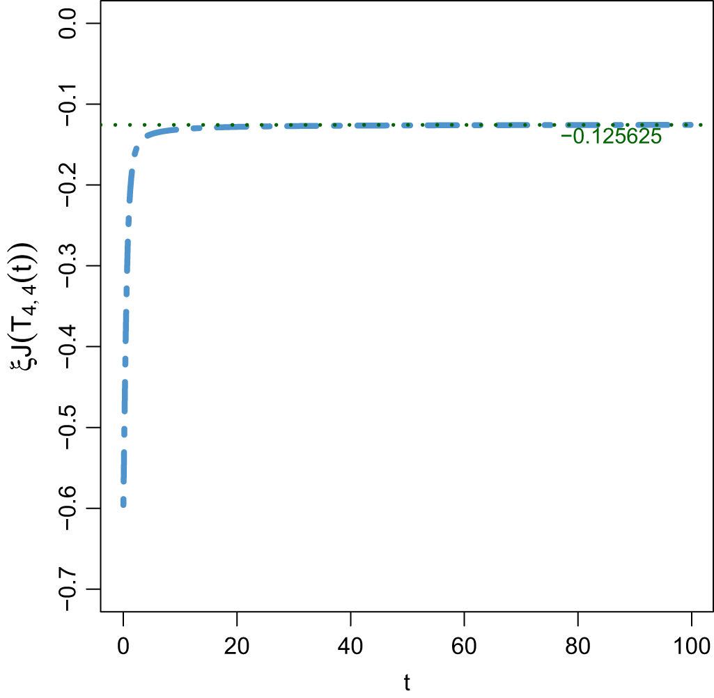


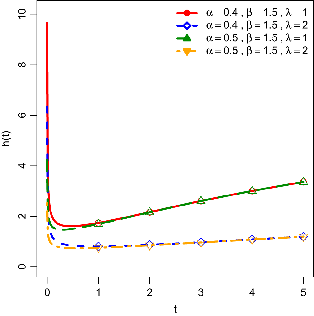

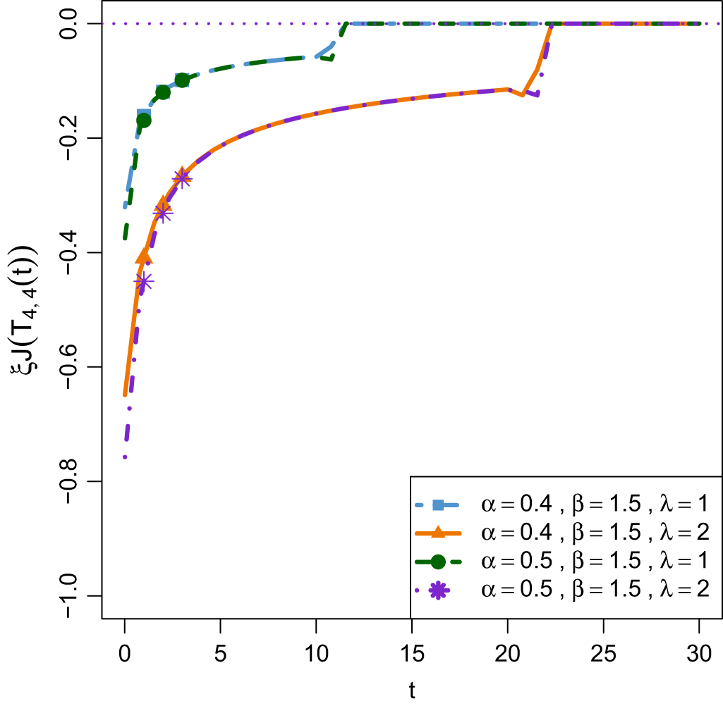

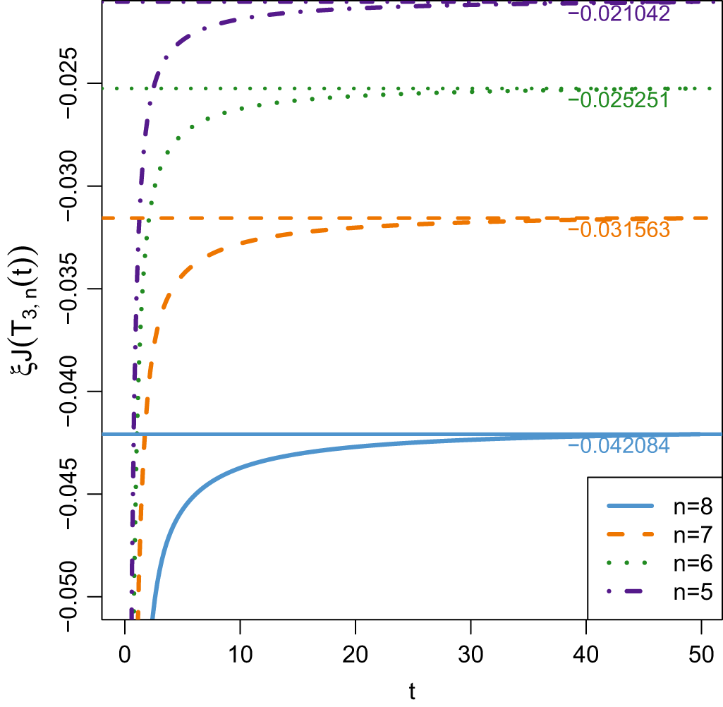


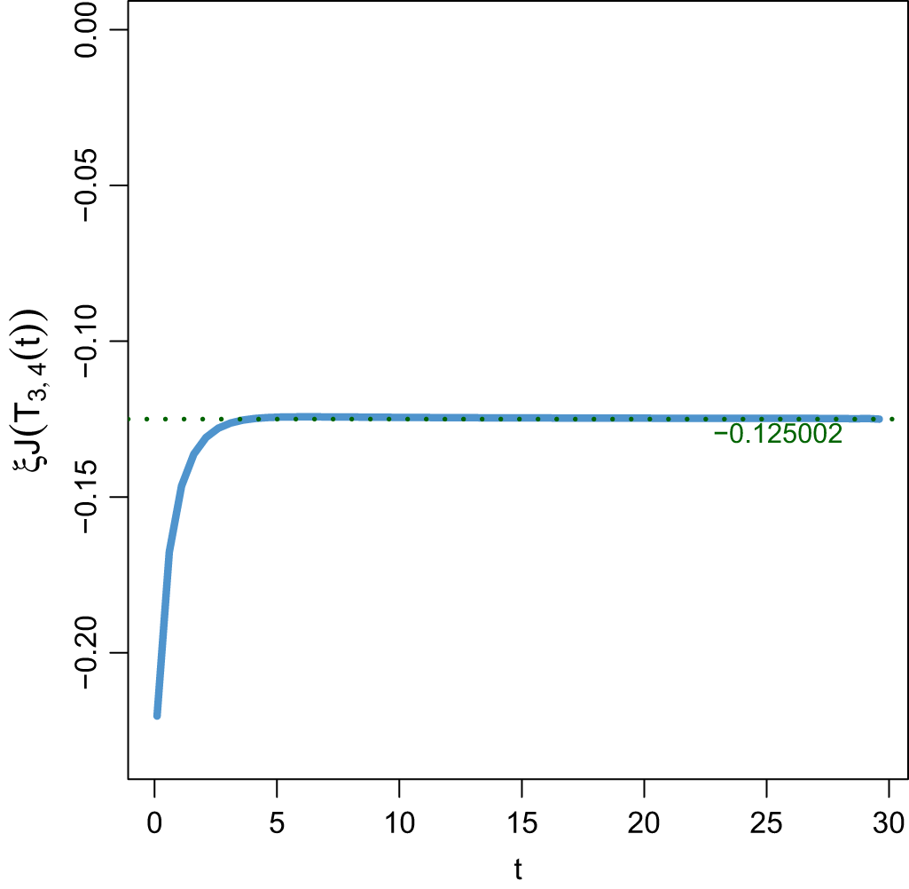


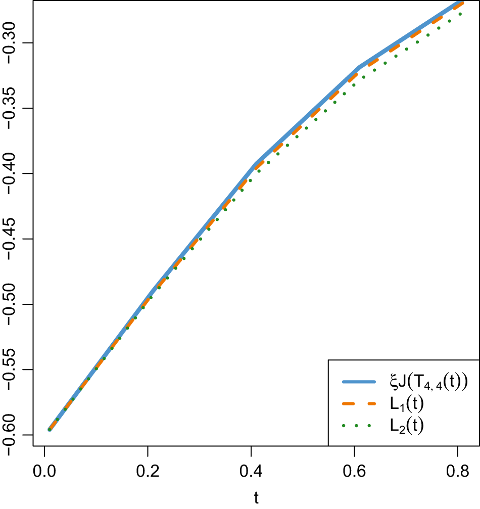


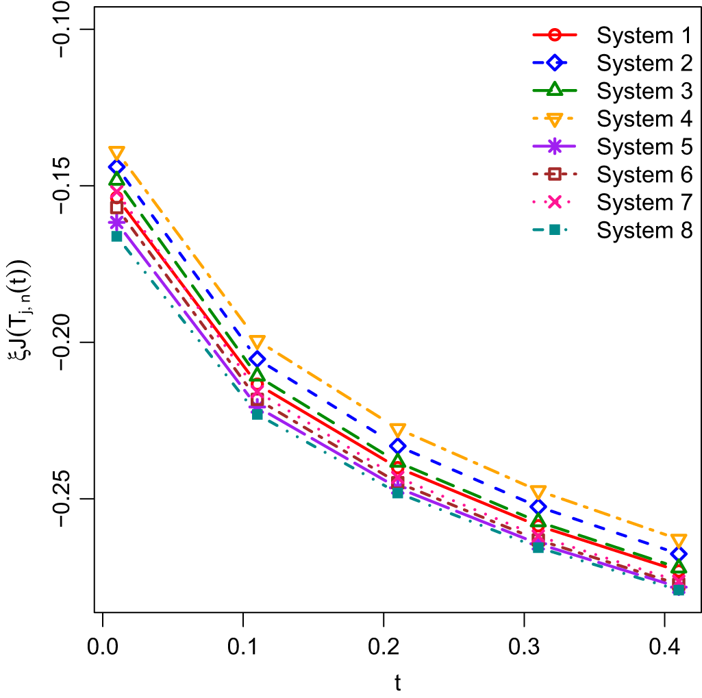


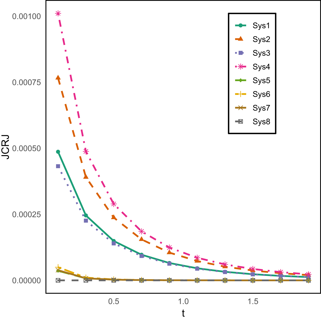


 Open access