2.1. Configuration and governing equations

We consider the flow past a two-dimensional single aerofoil of semi-chord $b = c/2,$ as sketched in figure 1. The flow is taken to be inviscid, non-heat-conducting and a compressible perfect gas. Neglecting volumetric forces, as well as thermal and mass diffusion the conservation of mass, momentum and energy can be written, respectively, as

(2.1a–c)\begin{equation} \frac{\partial \rho}{\partial t} + \boldsymbol{\nabla} \boldsymbol{\cdot} \left( \rho \boldsymbol{U} \right)=0, \quad \frac{\partial \boldsymbol{U}}{\partial t} + \boldsymbol{U} \boldsymbol{\cdot} \boldsymbol{\nabla} \boldsymbol{U} ={-}\frac{1}{\rho} \boldsymbol{\nabla} p, \quad \frac{\partial s}{\partial t} + \boldsymbol{U}\boldsymbol{\cdot} \boldsymbol{\nabla} s = 0, \end{equation}

where $\rho$ is the density, $p$ is the pressure, $\boldsymbol {U}$ is the velocity, $s$ is the specific entropy and $t$ is the time.

Figure 1.

Aerofoil of semi-chord $b$ at incidence angle $\alpha$ encountering a convected entropy disturbance.

We suppose that the flow upstream consists of a uniform component of velocity $U_{\infty },$ density $\rho _{\infty }$ and speed of sound $a_{\infty },$ on which there is superimposed a small unsteady motion. Consequently, the flow can be decomposed into a steady mean, denoted by $(\boldsymbol {\cdot })_0$, and a perturbation component, denoted by $(\boldsymbol {\cdot })'.$

The equations governing the mean flow are

(2.2a,b)\begin{equation} \boldsymbol{\nabla} \boldsymbol{\cdot} \left( \rho_0 \boldsymbol{U}_0 \right)=0, \quad \rho_0 \boldsymbol{U}_0 \boldsymbol{\cdot} \boldsymbol{\nabla} \boldsymbol{U}_0 ={-} \boldsymbol{\nabla} p_0. \end{equation}

The mean flow is also assumed homentropic, i.e. $s_0=0,$ and irrotational, i.e. ${\boldsymbol {\nabla } \times \boldsymbol {U}_0=0}$. Under the irrotational assumption, there exists a potential function such that $\boldsymbol {U}_{0}=\boldsymbol {\nabla } \varPhi$. Furthermore, and because the flow is two-dimensional, we can define a compressible stream function $\varPsi$ as

(2.3)\begin{equation} \boldsymbol{\nabla} \times \left( \rho_{\infty} \varPsi \boldsymbol{e_3} \right) = \beta_{\infty} \rho_0 \boldsymbol{U}_0, \end{equation}

where the factor $\beta _{\infty }=\sqrt {1-M^{2}_{\infty }}$ $(M_{\infty }=U_{\infty }/a_{\infty })$ corresponds to a Prandtl–Glauert transformation (Ashley & Landahl Reference Ashley and Landahl1985) and $\boldsymbol {e_3}$ is the unit vector perpendicular to the $x_1 - x_2$ plane.

We assume that small-amplitude entropic disturbances are superimposed on the uniform flow (infinitely far upstream). These disturbances are convected downstream by the mean flow and interact with the aerofoil, which produces sound. Similar approaches have been employed (Myers Reference Myers1987; Tsai Reference Tsai1992; Myers & Kerschen Reference Myers and Kerschen1995, Reference Myers and Kerschen1997) in modelling gust–blade interaction. Neglecting squares of small quantities and subtracting out the mean flow equations, we obtain that the dynamics of the perturbation part is governed by

(2.4a)\begin{gather} \frac{\textrm{D}_0 \rho'}{\textrm{D}t} + \rho'\boldsymbol{\nabla} \boldsymbol{\cdot} \boldsymbol{U}_0 + \boldsymbol{\nabla} \boldsymbol{\cdot} \left( \rho_0 \boldsymbol{u}'\right) = 0, \end{gather}

(2.4b)\begin{gather}\frac{\textrm{D}_0 \boldsymbol{u}'}{\textrm{D}t} + \boldsymbol{u}' \boldsymbol{\cdot} \boldsymbol{\nabla} \boldsymbol{U}_0 + \frac{\rho'}{\rho_0}\boldsymbol{U}_0 \boldsymbol{\cdot} \boldsymbol{\nabla} \boldsymbol{U}_0 ={-} \frac{1}{\rho_0}\boldsymbol{\nabla} p', \end{gather}

(2.4c)\begin{gather}\frac{\textrm{D}_0 s'}{\textrm{D}t} = 0, \end{gather}

where $\textrm {D}_0/\textrm {D}t = \partial /\partial t + \boldsymbol {U}_0 \boldsymbol {\cdot } \boldsymbol {\nabla }$ is the material derivative with respect to the local mean flow. The perturbation density, pressure and entropy are related by the Gibbs equation, which leads to

(2.5)\begin{equation} \frac{\rho'}{\rho_0} = \frac{p'}{\gamma p_0} - \frac{s'}{c_{p}}, \end{equation}

where $\gamma$ is the ratio of the specific heat capacities of the gas at constant pressure $c_p$ and constant volume $c_v,$ i.e. $\gamma =c_p/c_v.$

2.2. Rapid distortion theory formulation

The generalisation of rapid distortion theory proposed by Goldstein (Reference Goldstein1978) provides a well-suited framework for solving (2.4). Goldstein (Reference Goldstein1978) showed that the analysis of the perturbation dynamics can be reduced to solving a single inhomogeneous wave equation by introducing the following splitting of the perturbation velocity and pressure:

(2.6)\begin{equation} \boldsymbol{u}' = \boldsymbol{\nabla} \phi + \boldsymbol{u}^{(H)} + \frac{s'}{2 c_p}\boldsymbol{U}_0, \end{equation}

and

(2.7)\begin{equation} p' ={-}\rho_0\frac{\textrm{D}_0 \phi}{\textrm{D}t}. \end{equation}

The perturbation velocity is represented as the sum of a component that is the gradient of an acoustic potential $\phi ,$ a homogeneous component $\boldsymbol {u}^{(H)}$ and a term proportional to the perturbation entropy $s'$. The homogeneous component, $\boldsymbol {u}^{(H)},$ satisfies a modified form of the linearised momentum equation:

(2.8)\begin{equation} \frac{\textrm{D}_0 \boldsymbol{u}^{(H)}}{\textrm{D}t} + \boldsymbol{u}^{(H)}\boldsymbol{\cdot} \boldsymbol{\nabla} \boldsymbol{U}_0 = 0, \end{equation}

and $s'$ satisfies the energy equation (2.4c). These equations can be integrated exactly using the method of characteristics if appropriate boundary conditions are provided (see § 2.3).

To determine the acoustic potential $\phi ,$ (2.6), (2.7) and (2.5) are substituted into (2.4a) to obtain the following inhomogeneous, convective wave equation:

(2.9)\begin{equation} \frac{\textrm{D}_0}{\textrm{D}t}\left( \frac{1}{a_0^{2}}\frac{\textrm{D}_0\phi}{\textrm{D}t} \right)- \frac{1}{\rho_0}\boldsymbol{\nabla} \boldsymbol{\cdot}\left( \rho_0 \boldsymbol{\nabla} \phi \right) =\frac{1}{\rho_0}\boldsymbol{\nabla} \boldsymbol{\cdot} \left( \rho_0 \boldsymbol{u}^{(H)} \right) - \frac{1}{2c_p}\frac{\partial s'}{\partial t}, \end{equation}

subject to boundary conditions

(2.10a)\begin{gather} \boldsymbol{\nabla}{\phi}\boldsymbol{\cdot} \boldsymbol{n} ={-}\boldsymbol{u}^{(H)}\boldsymbol{\cdot} \boldsymbol{n}, \quad \text{on }\varSigma, \end{gather}

(2.10b)\begin{gather}\phi \rightarrow 0, \quad \text{as } x_{1} \rightarrow - \infty, \end{gather}

where $\varSigma$ is the surface of the aerofoil and $a_0$ is the local speed of sound of the mean flow.

The decomposition given by (2.6) and (2.7) greatly simplifies the problem: a coupled system of four partial differential equations (PDEs) is transformed into three fully decoupled PDEs ((2.8) and (2.4c)) together with a wave equation (2.9) coupled to the aforementioned ones only through the source term. The former equations can be integrated analytically, as explained in § 2.3, and an approximated solution to the latter is proposed in § 3.

2.3. Time-periodic entropy fluctuations

Equations (2.8) and (2.4c) can be integrated exactly using the method of characteristics if appropriate boundary conditions are provided. Here, we set a time-periodic entropic perturbation far upstream of the form:

(2.11)\begin{equation} s'_{\infty}/ c_p = A_s \exp{\left( \mathrm{i}\left[ k_1 x_1 + k_2 x_2 - \omega t \right] \right)}, \end{equation}

where $k_1$ and $k_2$ are the wavenumbers of the perturbation in $x_1$ and $x_2,$ respectively, and $\omega$ is the angular frequency. The relation $k_1 = \omega /U_{\infty }$ is satisfied. Equation (2.4c) can be integrated to yield:

(2.12)\begin{equation} \frac{s'}{c_p} = A_s \exp\left({\mathrm{i}\left( \boldsymbol{k} \boldsymbol{\cdot} \boldsymbol{X} - \omega t \right)}\right), \end{equation}

where $\boldsymbol {k}= ( k_1, k_2 )^{\top }$ and $\boldsymbol {X}=( X_{\varPhi }, X_{\varPsi } )^{\top }$ are vectors containing, respectively, the entropy wavenumbers and mean-flow Lagrangian coordinates:

(2.13a,b)\begin{equation} X_{\varPhi} = \frac{ \varPhi + g(\varPhi,\varPsi) }{U_{\infty}}, \quad X_{\varPsi} = \frac{\varPsi}{\beta_{\infty}U_{\infty}}, \end{equation}

with

(2.14)\begin{equation} g(\varPhi, \varPsi) = \int_{-\infty}^{\varPhi}\left[ \frac{U_{\infty}^{2}}{U_0(\xi,\varPsi)^{2}} - 1 \right]\,\textrm{d}\xi \end{equation}

as the drift function and $U_0$ is the magnitude of the velocity vector $\boldsymbol {U}_0.$ Note that the drift function $g$ is singular along any streamline passing through a stagnation point.

Additionally, we assume that the disturbances of the mean flow far upstream of the body are purely entropic ($\boldsymbol {u}'_{\infty }=0).$ Using this assumption, the homogeneous components of the perturbation velocity, $\boldsymbol {u}^{(H)}$, are directly obtained in Lagrangian coordinates (Kerschen & Balsa Reference Kerschen and Balsa1981) as

(2.15a)\begin{gather} \frac{u_t^{(H)}}{U_\infty} ={-}\frac{A_s}{2} \frac{U_{\infty}}{U_0} \exp({\mathrm{i} \left( \boldsymbol{k} \boldsymbol{\cdot} \boldsymbol{X} - \omega t \right)}), \end{gather}

(2.15b)\begin{gather}\frac{u_n^{(H)}}{U_{\infty}} ={-}\beta_{\infty} \frac{A_s}{2} \frac{\rho_0 U_0}{\rho_{\infty} U_{\infty}} \frac{\partial g}{\partial \varPsi} \exp({\mathrm{i} \left( \boldsymbol{k} \boldsymbol{\cdot} \boldsymbol{X} - \omega t \right)}), \end{gather}

with $u^{(H)}_t$ and $u^{(H)}_n$ denoting the velocity components parallel and normal to a streamline, respectively.

The source term of (2.9) can now be obtained as

(2.16)\begin{equation} \mathcal{S}(\boldsymbol{x}, t) ={-}\frac{1}{\rho_0}\boldsymbol{\nabla} \boldsymbol{\cdot} \left( \rho_0 \boldsymbol{u}^{(H)} \right) - \frac{\mathrm{i} \omega}{2c_p} s' = \hat S(\boldsymbol{x};\omega) \exp{\left( -\mathrm{i} \omega t \right)}, \end{equation}

where

(2.17) $$\begin{align} \hat S(\varPhi, \varPsi; \omega) &= \frac{A_s}{2} \left[{-}2 \frac{U_{\infty}^{2}}{U_0}\frac{\partial {U_0}}{\partial {\varPhi}} + 2 \beta_{\infty}^{2}\frac{\rho_0 U_0^{2}}{\rho_{\infty}^{2}} \frac{\partial {\rho_0}}{\partial {\varPsi}}\frac{\partial {g}}{\partial {\varPsi}} \right. + \beta_{\infty}^{2}\frac{\rho_0^{2} U_0^{2}}{\rho_{\infty}^{2}} \frac{\partial {{}^{2}g}}{\partial {\varPsi^{2}}} + \mathrm{i} k_1 {U_{\infty}}\nonumber\\ &\quad \times \left( \frac{U_{\infty}^{2}}{U_0^{2}} - 1 + \beta_{\infty}^{2}\frac{\rho_0^{2} U_0^{2}}{\rho_{\infty}^{2}U_{\infty}^{2}}\frac{\partial {g}}{\partial {\varPsi}} \frac{\partial {g}}{\partial {\varPsi}} \right) + \mathrm{i} k_2 \beta_{\infty}\frac{\rho_0^{2} U_0^{2}}{\rho_{\infty}^{2}{U_{\infty}}}\frac{\partial {g}}{\partial {\varPsi}} \left. \vphantom{\frac{\rho_0^{2} U_0^{2}}{{M_{\infty}}}\frac{\partial {g}}{\partial {\varPsi}}} \right] \exp({\mathrm{i} \boldsymbol{k} \boldsymbol{\cdot} \boldsymbol{X}}). \end{align}$$

The time-harmonic dependence of the source term and boundary conditions of (2.9) allow us to write a solution in the form $\phi (\boldsymbol {x},t) = \hat \phi (\boldsymbol {x}) \exp {( -\mathrm {i} \omega t )}.$ Introducing now the acoustic wavenumber $\kappa _0=\omega /a_0$ and local Mach number $\boldsymbol {M}_0=\boldsymbol {U}_0/a_0,$ this equation can be rewritten as

(2.18)\begin{equation} \left[ \nabla^{2} + \left( \kappa_0 + \mathrm{i} \boldsymbol{M}_0 \boldsymbol{\cdot} \boldsymbol{\nabla} \right)^{2} \right]\hat \phi + \mathcal{L}_{0}\left(\hat \phi \right) = \hat S, \end{equation}

with

(2.19)$$\begin{gather} \mathcal{L}_{0}\left(\hat \phi \right) = \boldsymbol{\nabla} \hat \phi \boldsymbol{\cdot} \left(-\boldsymbol{M}_0 \boldsymbol{\cdot} \boldsymbol{\nabla} \boldsymbol{M}_0 + \boldsymbol{\nabla} \ln \rho_0 + \boldsymbol{M}_0( \boldsymbol{M}_0 \boldsymbol{\cdot} \boldsymbol{\nabla} \ln a_0) \right)\nonumber\\ +\, \mathrm{i} \hat \phi \left( \boldsymbol{M}_0\boldsymbol{\cdot} \boldsymbol{\nabla} \kappa_0 - \kappa_0\boldsymbol{M}_0\boldsymbol{\cdot} \boldsymbol{\nabla} \ln a_0 \right). \end{gather}$$

Note that the sign of (2.9) has been reversed in (2.18), hence the definition of the source term in (2.16) as minus its right-hand side.

To set the context of the analysis, we now summarise the assumptions used up to this point. Viscous effects and, thus, the presence of boundary layers are neglected. Boundary layers are expected to enhance the shear of entropy waves close to the walls, especially in confined flows. Second, the magnitude of the entropic and acoustic waves is assumed to be small compared to the mean flow so that the governing equations can be linearised. The mean flow is assumed homentropic and irrotational. Finally, the mean flow is taken to be two-dimensional so that a streamfunction can be defined. This allows us to obtain the entropy distribution as in (2.12) and, thus, the source term given by (2.17).

3.1. Born approximation

Let us decompose the local Mach number and acoustic wavenumber on the left-hand side of (2.18) into an homogeneous and inhomogeneous part, such as

(3.1a,b)\begin{equation} \boldsymbol{M}_0(\boldsymbol{x}) = M_{\infty} \boldsymbol{e}_1 +\boldsymbol{M}_{\varDelta}(\boldsymbol{x}), \quad \kappa_0(\boldsymbol{x}) = \kappa_{\infty} + \kappa_{\varDelta}(\boldsymbol{x}), \end{equation}

where $\boldsymbol {e}_{1}$ denotes the unit vector in the $x_1$-direction and $\kappa _{\infty }=\omega /a_{\infty }$ is the acoustic wavenumber in the far field. Equation (2.18) can now be recast as

(3.2)\begin{equation} \left[ \nabla^{2} + \left( \kappa_{\infty}+ \mathrm{i} M_{\infty}\frac{\partial}{\partial x_1}\right)^{2} \right]\hat \phi + \mathcal{L}_{\varDelta}\left( \hat \phi \right) = \hat S, \end{equation}

where the operator $\mathcal {L}_{\varDelta }$ is given by

(3.3)\begin{align} \mathcal{L}_{\varDelta}\left({\cdot}\right) = \left[ \left( \kappa_{\varDelta} + \mathrm{i} \boldsymbol{M}_{\varDelta} \boldsymbol{\cdot} \boldsymbol{\nabla} \right)^{2} + 2 \left( \kappa_{\infty} + \mathrm{i} M_{\infty} \partial/\partial x_1\right) \left(\kappa_{\varDelta} + \mathrm{i} \boldsymbol{M}_{\varDelta} \boldsymbol{\cdot} \boldsymbol{\nabla}\right)\right]\left({\cdot}\right) + \mathcal{L}_0\left({\cdot}\right). \end{align}

This operator captures the effect of the mean-flow inhomogeneity on the acoustic propagation. If its effect is weak, we can neglect it and assume that the source term acts on the uniform portion of the mean flow, such that

(3.4)\begin{equation} \left[ \nabla^{2} + \left( \kappa_{\infty} + \mathrm{i} M_{\infty}\frac{\partial}{\partial x_1}\right)^{2} \right]\hat \phi_{\infty} = \hat S. \end{equation}

This approximation can be further improved by considering the effect of the inhomogeneity on the acoustic field as a second-order source term correction, i.e. $\hat \phi = \hat \phi _{\infty } + \hat \phi _{\varDelta },$ where $\hat \phi _{\varDelta }$ satisfies

(3.5)\begin{equation} \left[ \nabla^{2} + \left( \kappa_{\infty} + \mathrm{i} M_{\infty}\frac{\partial}{\partial x_1}\right)^{2} \right]\hat \phi_{\varDelta} ={-}\mathcal{L}_{\varDelta}\left( \hat \phi_{\infty} \right). \end{equation}

The above is known as the first-order Born approximation (Snieder & Van Wijk Reference Snieder and Van Wijk2015, Ch. 23). Chew (Reference Chew1995, Ch. 8) established the regime of validity of the Born approximation for the Helmholtz equation, and showed that it was especially pertinent at low frequencies. In Appendix A, we use a similar approach to show that the Born approximation limits of validity for (3.2) are given by

(3.6a–g)$$\begin{gather} He^{2} \; \delta \kappa ^{2} \ll 1, \quad He \; M_{\infty} \; \delta\kappa \; \delta M \ll 1,\quad M_{\infty}^{2} \; \delta M^{2} \ll 1, \quad He^{2} \; \delta \kappa \ll 1,\nonumber\\ He \; M_{\infty} \; \delta M \ll 1, \quad He \; M_{\infty} \; \delta \kappa \ll 1 \quad \text{and} \quad M_{\infty}^{2} \; \delta M \ll 1, \end{gather}$$

where $\delta \kappa$ and $\delta M$ represent the order of the normalised wavenumber and Mach number inhomogeneity, respectively, and $He=\omega b/a_{\infty }$ is the Helmholtz number. This shows that the Born approximation is perfectly suited to problems at low frequencies, low Mach numbers and with weak mean-flow inhomogeneities. In § 4, we simplify the source term by assuming that the mean flow is a small perturbation to a uniform flow. Equation (3.6a–g) shows that if this condition holds, the Born approximation is valid for any subsonic Mach number and for low-to-moderate frequencies. At high frequencies, the Born approximation is not suitable even for weak scatterers. This conclusion, which was obtained using simple dimensional analysis, was already postulated by Myers & Kerschen (Reference Myers and Kerschen1997) who showed the importance of accurately capturing the vortical-sound coupling between the leading and trailing edges to correctly predict the radiated far field at high frequencies. The present analysis also shows that this methodology can be used for aerofoils with larger thickness, camber or incoming angle of attack than those considered in the aforementioned studies, provided that the frequency and Mach number are sufficiently low.

To illustrate the solution method, we now consider the zeroth-order approximation, i.e. $\hat \phi =\hat \phi _{\infty }$. The first-order correction, $\hat \phi _{\varDelta }$, can be obtained equivalently by accordingly replacing the source term in the following procedure. A Lorentz-type transformation of the form:

(3.7)\begin{equation} \left. \begin{aligned} \tilde x_1 & = x_1/\beta_{\infty}, \quad \tilde x_2 = x_2, \quad \beta_{\infty} = \sqrt{1 - M_{\infty}^{2}},\\ \tilde \kappa_{\infty} & = \kappa_{\infty}/\beta_{\infty}, \quad \tilde \phi = \hat \phi \exp({\mathrm{i} \tilde \kappa_{\infty} {M_{\infty}} \tilde x_1}), \end{aligned} \right\} \end{equation}

is now used to transform (3.4) into the Helmholtz equation, that is

(3.8a,b)\begin{equation} \left[ \tilde \nabla^{2} + \tilde \kappa_{\infty}^{2} \right] \tilde \phi = \tilde S, \quad \tilde S = \hat S \exp({\mathrm{i} \tilde \kappa_{\infty} {M_{\infty}} \tilde x_1}). \end{equation}

Equation (3.8a,b) has been widely studied and can be solved using techniques available in the literature. Here, we propose a solution using the compact Green's function approach (Howe Reference Howe1975, Reference Howe2003) as outlined in § 3.2.

3.2. Integral solution using the compact Green's function method

Consider the Green's function $G(\tilde {\boldsymbol {x}},\tilde {\boldsymbol {y}})$ satisfying

(3.9a,b)\begin{equation} \left[ \tilde \nabla^{2} + \tilde \kappa_{\infty}^{2} \right] G(\tilde{\boldsymbol{x}},\tilde{\boldsymbol{y}}) = \delta(\tilde{\boldsymbol{x}} - \tilde{\boldsymbol{y}}), \quad \frac{\partial G}{\partial \tilde{\boldsymbol{n}}} - \mathrm{i} \tilde{\kappa}_{\infty}{M_{\infty}} \tilde{n}_1 G=0, \quad \text{on }\varSigma, \end{equation}

where $\delta$ is the Dirac delta function. The physical meaning of this Green's function is the solution owing to a point source of unit strength at a point $\tilde {\boldsymbol {y}},$ influenced by the surface $\varSigma .$ In an unbounded fluid, this Green's function must also satisfy the radiation condition that energy delivered to the fluid by the source radiates away from the source, i.e. the solution must exhibit outgoing wave behaviour.

Consider the closed surface ${S}$ bounding the spatial domain ${V}$, as depicted in figure 2. This surface comprises three subsurfaces: ${S} = \varSigma \cup {S}_{\infty } \cup {W},$ where $\varSigma$ and ${W}$ are surfaces surrounding the aerofoil and the wake (the portion of the streamline that goes from the trailing edge to infinity downstream), respectively, and ${S}_{\infty }$ is a surface very far from the aerofoil. We denote by $\boldsymbol {n}$ the inward unit normal to ${S}.$ Multiplying (3.8a,b) by the Green's function defined by (3.9a,b) and integrating over the domain ${V},$ we obtain after some manipulations (see Appendix B) the following integral solution for the acoustic potential:

(3.10)$$\begin{gather} \tilde \phi(\tilde{\boldsymbol{x}}) = \int_{{V}} G(\tilde{\boldsymbol{x}}, \tilde{\boldsymbol{y}})\tilde{S}(\,\tilde{\boldsymbol{y}})\,\textrm{d}{V}(\,\tilde{\boldsymbol{y}}) + \int_{\varSigma + {W}} G(\tilde{\boldsymbol{x}}, \tilde{\boldsymbol{y}}) \frac{\partial \hat \phi}{\partial \tilde{\boldsymbol{n}}}(\,\tilde{\boldsymbol{y}}) \exp({\mathrm{i} \tilde \kappa_{\infty} {M_{\infty}} \tilde y_1})\,\textrm{d}{S}(\,\tilde{\boldsymbol{y}})\nonumber\\ - \int_{{W}} \tilde \phi(\,\tilde{\boldsymbol{y}})\left( \frac{\partial G}{\partial \tilde{\boldsymbol{n}}}(\tilde{\boldsymbol{x}},\tilde{\boldsymbol{y}}) - \mathrm{i} \tilde{\kappa}_{\infty}{M_{\infty}} \tilde{n}_1 G(\tilde{\boldsymbol{x}},\tilde{\boldsymbol{y}})\right) \textrm{d}{S}(\,\tilde{\boldsymbol{y}}). \end{gather}$$

The integrals in ${S}_{\infty }$ vanish (see Wu & Lee Reference Wu and Lee1994). Along the wake, the source term can be singular, hence the acoustic potential can become discontinuous. The line integrals along the wake are retained to ensure the continuity of the pressure and normal velocity across it, as well as the Kutta condition at the trailing edge. In § 4, we show that in the thin-aerofoil limit this integral disappears. For simplicity's sake, we neglect it hereafter. The integral term over $\varSigma$ represents the contribution to the acoustic field generated to satisfy the slip boundary condition on the body. For convenience, the surface $\varSigma$ is further decomposed into two surfaces : $\varSigma = \varSigma ^{+} \cup \varSigma ^{-},$ where $\varSigma ^{+}$ and $\varSigma ^{-}$ denote the upper and lower side of the aerofoil, respectively, going from the leading to the trailing edge.

Figure 2.

Schematic of the region ${V}$ used in the derivation of the integral equation (3.10). Here, ${S}$ is the surface bounding ${V}$: ${S} = \varSigma \cup {S}_{\infty } \cup {W}$.

An approximate solution to (3.9a,b) (to order $(\tilde \kappa _{\infty } b)^{2}$) is given by the compact Green's function approach of Howe (Reference Howe1975, Reference Howe2003) as

(3.11)\begin{equation} G(\tilde{\boldsymbol{x}}, \tilde{\boldsymbol{y}}; \omega) ={-}\frac{\mathrm{i}}{4} \left[ \mathcal{H}_0^{(1)}(\tilde \kappa_{\infty}|\tilde{\boldsymbol{x}}|) + \mathcal{H}_1^{(1)}(\tilde \kappa_{\infty}|\tilde{\boldsymbol{x}}|) \tilde \kappa_{\infty} \frac{\tilde{x}_j Y_j(\,\tilde{\boldsymbol{y}})}{|\tilde{\boldsymbol{x}}|} \right], \end{equation}

for an observer at $\tilde {\boldsymbol {x}}$ and source at $\tilde {\boldsymbol {y}}.$ Here, $\mathcal {H}_0^{(1)}$ and $\mathcal {H}_1^{(1)}$ are the Hankel functions of the first kind for the zeroth and first order, respectively. The double index $j=1,2$ implies summation. The Kirchhoff vector $Y_j \equiv y_j - \varphi _j^{*}(\,\tilde {\boldsymbol {y}})$ satisfies

(3.12)\begin{equation} \tilde \nabla^{2}Y_j=0, \end{equation}

subject to

(3.13)\begin{equation} \frac{\partial Y_j}{\partial \tilde{\boldsymbol{n}}} -\mathrm{i}\tilde \kappa_{\infty} M_{\infty}Y_j \tilde n_1=0, \quad \text{on } \varSigma. \end{equation}

The function $\varphi _j^{*}(\,\tilde {\boldsymbol {y}})$ represents the effect of the solid boundary on the acoustic response (see Howe Reference Howe2003 for a detailed description). Any acoustic source placed far from the aerofoil will be virtually not affected by it. To reflect this, we require that $\varphi _j^{*}(\,\tilde {\boldsymbol {y}})$ decays with distance from $\varSigma .$

The acoustic potential field is then obtained by substituting the compact Green's function given by (3.11) into (3.10) to yield:

(3.14) $$\begin{align} \tilde \phi(\tilde{\boldsymbol{x}}) &= \frac{-\textrm{i}}{4} \left[ \mathcal{H}_0^{(1)}(\tilde \kappa_{\infty}|\tilde{\boldsymbol{x}}|) \left( \int_{V} \tilde S(\,\tilde{\boldsymbol{y}}) \; \textrm{d}V(\,\tilde{\boldsymbol{y}}) + \int_{\varSigma} \frac{\partial \hat \phi}{\partial \tilde{\boldsymbol{n}}}(\,\tilde{\boldsymbol{y}}) \exp({\mathrm{i} \tilde \kappa_{\infty} {M_{\infty}} \tilde y_1})\, \textrm{d} S(\,\tilde{\boldsymbol{y}}) \right)\right.\nonumber\\ &\quad + \left.\tilde \kappa_{\infty} \frac{\tilde x_j }{|\tilde{\boldsymbol{x}}|} \mathcal{H}_1^{(1)}(\tilde \kappa_{\infty}|\tilde{\boldsymbol{x}}|) \left( \int_{V} Y_j(\,\tilde{\boldsymbol{y}}) \tilde S(\,\tilde{\boldsymbol{y}}) \; \textrm{d}V(\,\tilde{\boldsymbol{y}}) + \int_{\varSigma} Y_j(\,\tilde{\boldsymbol{y}}) \frac{\partial \hat \phi}{\partial \tilde{\boldsymbol{n}}}(\,\tilde{\boldsymbol{y}}) \exp({\mathrm{i} \tilde \kappa_{\infty} {M_{\infty}} \tilde y_1}) \, \textrm{d} S(\,\tilde{\boldsymbol{y}}) \right) \right]. \end{align}$$

All the terms involving the observer position are moved outside of the integrals in (3.14) and, thus, the acoustic potential can be expressed as a linear combination of three basic components:

(3.15)\begin{equation} \hat \phi(\tilde{\boldsymbol{x}}) = \alpha_0 \; \phi_0(\tilde{\boldsymbol{x}}) + \alpha_1 \; \phi_1(\tilde{\boldsymbol{x}}) + \alpha_2 \; \phi_2(\tilde{\boldsymbol{x}}), \end{equation}

with

(3.16a)\begin{gather} \alpha_0 = \int_{{V}} \tilde S(\,\tilde{\boldsymbol{y}}) \, \textrm{d} V(\,\tilde{\boldsymbol{y}}) + \int_{{\varSigma}} \frac{\partial \hat \phi}{\partial \tilde{\boldsymbol{n}}}(\,\tilde{\boldsymbol{y}}) \exp({\mathrm{i} \tilde \kappa_{\infty} {M_{\infty}} \tilde y_1}) \, \textrm{d} S(\,\tilde{\boldsymbol{y}}), \end{gather}

(3.16b)\begin{gather}\alpha_j = \tilde \kappa_{\infty} \left( \int_{{V}} Y_j(\,\tilde{\boldsymbol{y}}) \tilde S(\,\tilde{\boldsymbol{y}}) \, \textrm{d} V(\,\tilde{\boldsymbol{y}}) + \int_{{\varSigma}} Y_j(\,\tilde{\boldsymbol{y}}) \frac{\partial \hat \phi}{\partial \tilde{\boldsymbol{n}}}(\,\tilde{\boldsymbol{y}}) \exp({\mathrm{i} \tilde \kappa_{\infty} {M_{\infty}} \tilde y_1}) \, \textrm{d} S(\,\tilde{\boldsymbol{y}}) \right), \end{gather}

and

(3.17a)\begin{gather} \phi_0(\tilde{\boldsymbol{x}}) ={-}\frac{\mathrm{i}}{4} \left[\mathcal{H}_0^{(1)}(\tilde \kappa_{\infty}|\tilde{\boldsymbol{x}}|) \right] \exp({-\mathrm{i} \tilde \kappa_{\infty}M_{\infty}\tilde x_1}), \end{gather}

(3.17b)\begin{gather}\phi_j(\tilde{\boldsymbol{x}}) ={-}\frac{\mathrm{i}}{4} \left[\frac{\tilde x_j }{|\tilde{\boldsymbol{x}}|} \mathcal{H}_1^{(1)}(\tilde \kappa_{\infty}|\tilde{\boldsymbol{x}}|) \right] \exp({-\mathrm{i} \tilde \kappa_{\infty}M_{\infty}\tilde x_1}), \end{gather}

with $j = 1, 2.$

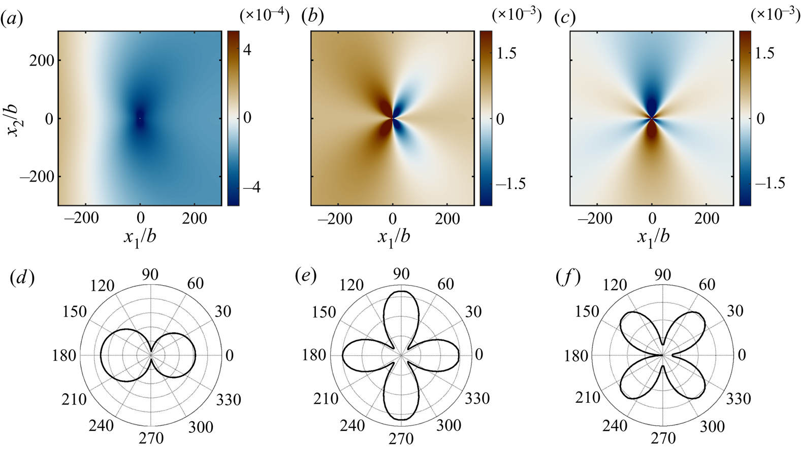
Figure 3 shows these three components which are a monopole, a dipole in the horizontal axis and a dipole in the vertical axis. The velocity potential field, $\hat \phi (\boldsymbol {x}),$ will then depend on the geometry of the field through the weighting terms $\alpha _0,$ $\alpha _1$ and $\alpha _2$ in (3.15). The three components are affected by the Doppler factor $\exp ({-\mathrm {i} \tilde \kappa _{\infty }M_{\infty }\tilde x_1}),$ which causes the wavelength of the potential propagating in the forward direction to be shortened by the motion whereas the wavelength of the potential propagating in the rear direction is lengthened.

Figure 3.

Components of the solution of the acoustic potential, $\hat \phi ,$ for a flow $M_{\infty }=0.2$ and $He = 0.05:$ (a,d) $\phi _0;$ (b,e) $\phi _1;$ and (c,f) $\phi _2.$ (a–c) Real part and (d–f) directivity.

The pressure field is then obtained from these three components using (2.7). If the observer is sufficiently far from the aerofoil, the mean flow velocity and density can be assumed uniform and the pressure field simplifies to

(3.18)\begin{equation} p'= \rho_{\infty}\left[ \mathrm{i} \omega \hat \phi - U_{\infty} \frac{\partial \hat \phi}{\partial x_1}\right], \end{equation}

which shows that the pressure field is given as a combination of the acoustic potential and its derivative in the streamwise direction $\partial {\hat \phi }/{\partial x_1}.$ The streamwise derivatives for the three potential components are given by

(3.19a)\begin{gather} \frac{\partial \phi_0}{\partial x_1} ={-}\frac{\kappa_{\infty}}{\beta_{\infty}^{2}}\left[ \mathrm{i} M_{\infty}\phi_0 + \phi_1 \right], \end{gather}

(3.19b)\begin{gather}\frac{\partial \phi_1}{\partial x_1} ={-}\frac{\kappa_{\infty}}{\beta_{\infty}^{2}}\left[ \mathrm{i} M_{\infty}\phi_1 - \frac{\mathrm{i}}{4}\left( \frac{\tilde x_1^{2}}{|\tilde{\boldsymbol{x}}|^{2}}\mathcal{H}_2^{(1)}(\tilde \kappa_{\infty}|\tilde{\boldsymbol{x}}|) - \frac{1}{|\tilde{\boldsymbol{x}}|}\frac{\mathcal{H}_1^{(1)}(\tilde \kappa_{\infty}|\tilde{\boldsymbol{x}}|)}{\tilde \kappa_{\infty}} \right) \exp({-\mathrm{i} \tilde \kappa_{\infty}M_{\infty}\tilde x_1}) \right], \end{gather}

(3.19c)\begin{gather}\frac{\partial \phi_2}{\partial x_1} ={-}\frac{\kappa_{\infty}}{\beta_{\infty}^{2}}\left[ \mathrm{i} M_{\infty}\phi_2 - \frac{\mathrm{i}}{4}\left( \frac{\tilde x_1 \tilde x_2}{|\tilde{\boldsymbol{x}}|^{2}}\mathcal{H}_2^{(1)}(\tilde \kappa_{\infty}|\tilde{\boldsymbol{x}}|) \right) \exp({-\mathrm{i} \tilde \kappa_{\infty}M_{\infty}\tilde x_1}) \right]. \end{gather}

where $\mathcal {H}_2^{(1)}$ is the Hankel function of first kind and second order. These functions are depicted in figures 4 and 5 for two different Helmholtz numbers. The term $\mathrm {i} M_{\infty }$ arises from the Doppler factor and causes the sound radiated in the forward direction to be amplified whereas the sound propagating in the rear direction is attenuated. For the first component, the monopole $\phi _0,$ its derivative additionally includes a dipole whose wavelength and amplitude are accordingly modulated by the Doppler effect. For the second component, the dipole along the horizontal axis $\phi _1,$ its derivative additionally includes two terms: a flattened horizontal dipole and a term with a omnidirectional directivity, and that decays with distance and frequency faster than a monopole. Figure 4(b,e) and 5(b,e) show how at high frequencies the dominant contribution is the flattened dipole, while at lower frequencies both contributions are as important and combine to form a directivity pattern comprising four lobes along the two main axes. Finally, for the third component, the vertical dipole $\phi _2,$ its derivative is a quadrupole also affected by the Doppler effect (stronger sound amplitude in the forward direction).

Figure 4.

Streamwise derivative of the components of the acoustic potential, $\partial {\hat \phi }/{\partial x_1},$ for a flow $M_{\infty }=0.2$ and $He = 0.05:$ (a,d) $\partial {\phi _0}/{\partial x_1};$ (b,e) $\partial {\phi _1}/{\partial x_1};$ and (c,f) $\partial {\phi _2}/{\partial x_1}.$ (a–c) Real part and (d–f) directivity.

Figure 5.

Streamwise derivative of the components of the acoustic potential, $\partial {\hat \phi }/{\partial x_1},$ for a flow $M_{\infty }=0.2$ and $He = 0.001:$ (a,d) $\partial {\phi _0}/{\partial x_1};$ (b,e) $\partial {\phi _1}/{\partial x_1};$ and (c,f) $\partial {\phi _2}/{\partial x_1}.$ (a–c) Real part and (d–f) directivity.

The results presented up to this point constitute a contribution of the present work. The combination of the Born approximation with (2.9) allows the integral solution given by (3.10) to be obtained. This solution is valid within the limits summarised at the end of § 2 and those given by (3.6a–g). The solution expands the range of validity of analytical solutions beyond that available in the existing literature, because it allows aerofoils outside the scope of thin-aerofoil theory to be described. Finally, we restrict the analysis to low acoustic wavelengths ($He^{2} \ll 1$) so that the computation of the Green's functions is greatly simplified and (3.14) is obtained. This expression can be readily integrated numerically provided that the details of the mean flow are available.

5.1. Numerical results

We first compute a numerical solution of the two-dimensional compressible Euler equations as a benchmark for the model. Both the steady and linearised Euler equations are solved using the finite element method (Donea & Huerta Reference Donea and Huerta2003) implemented using the open-source computing platform FEniCS (Logg et al. Reference Logg2012; Alnæs et al. Reference Alnæs, Blechta, Hake, Johansson, Kehlet, Logg, Richardson, Ring, Rognes and Wells2015).

The mean flow is obtained as the solution of the steady compressible Euler equations in conservation variables. The equations are discretised in space using a continuous Galerkin formulation stabilised using the least-squares method (Donea & Huerta Reference Donea and Huerta2003). The discretised nonlinear problem is solved using a fully-implicit, pseudo-time-stepping algorithm (Crivellini, D'Alessandro & Bassi Reference Crivellini, D'Alessandro and Bassi2013). The algorithm adapts the local time step every iteration so that it is inversely proportional to the local residuals. When the residuals are small, the time step becomes large, the unsteady term negligible and the algorithm effectively behaves as the Newton method, exhibiting quadratic convergence. The global residuals (in norm-2) for all the results presented hereafter are lower than $10^{-9}.$ The results are typically obtained in less than 100 iterations. At the aerofoil boundary we require the fluid to satisfy the slip boundary condition. At the inlet we impose uniform velocity and density, and at the outlet we impose uniform pressure. The meshes used in this study are fully unstructured and contain approximately 200 000 triangular elements. The approximation polynomials are quadratic. The domain is a square with the length of a side being $26b.$

Figure 6 depicts the mean flow obtained numerically. At the leading edge of the aerofoil, the flow quickly decelerates from the upstream velocity to being stagnant. It then accelerates until the point of maximum thickness of the aerofoil and gently decelerates thereafter until the trailing edge. Note that for Joukowsky aerofoils, a second stagnation point does not exist there (in contrast with realistic aerofoils). At the point of largest velocity, its increase never exceeds $20\,\%$ of the unperturbed velocity. Therefore, the main acceleration occurs in the region around the stagnation point at the leading edge. This velocity variation translates to the density and speed of sound. The speed of sound does not exceed $2\,\%$ of the unperturbed one in any case. The variation of density is larger, reaching variations of $4\,\%$ at the leading edge for $M_{\infty }=0.5,$ but remains low enough to neglect them in the analytical model.

Figure 6.

Normalised density $\rho _0/\rho _{\infty },$ local Mach number $M_0=U_0/a_0$ and normalised speed of sound $a_0/a_{\infty }$ for a symmetric aerofoil at (a–c) ${M_{\infty }}=0.2$ and (d–f) ${M_{\infty }}=0.5.$

We now turn our attention to the acoustic problem. The linearised compressible Euler equations are formulated in primitive variables and recast in the frequency domain. Then, they are spatially discretised using the discontinuous Galerkin method (Bassi & Rebay Reference Bassi and Rebay1997; Cockburn & Shu Reference Cockburn and Shu2001). The discretisation leads to a linear problem that is solved using the sparse linear solver MUMPS (Amestoy et al. Reference Amestoy, Duff, Koster and L'Excellent2001, Reference Amestoy, Guermouche, L'Excellent and Pralet2006). A perfectly matched layer (PML) (Hu Reference Hu2001) was added to the domain to damp any incoming acoustic wave. To enforce the incoming entropy waves, an incident density fluctuation was superimposed to the reflected solution in the PML (Özyörük Reference Özyörük2009). A slip boundary condition is used on the aerofoil.

The current implementation of the finite element method allows for approximation polynomials whose order range $p=0 - 5.$ The bulk of the simulations are carried out using quadratic elements $p=2$. However, to assess the accuracy of the results, simulations with cubic elements were performed for the highest frequencies showing the independence of the results to the order of the polynomials. Additionally, a mesh convergence study was performed showing that 20 points per entropy wavelength are sufficient to obtain mesh-independent results. The final mesh used for the study is unstructured and is composed approximately of 150 000 triangular elements. The domain is again a square. The length of the domain is varied from $20b$ to $40b.$ All the domains are extended by a PML of length $5b.$ The PML coefficients are $\sigma _m=6$ and $\beta =2$ (as defined by Hu Reference Hu2001). For the highest frequencies considered here, the simulations are independent of the size of the domain. However, for the lowest frequency (corresponding to $He=0.001$), small variations are observed for different domains. This indicates that the simulation for this frequency is not fully converged in domain size (larger domains are beyond our current computational capabilities). The variations of the acoustic directivity with different sizes are small enough to assure that the results will not change dramatically for larger domains. Note that the effect of the PML layer was ruled out by running several simulations with different sets of PML parameters for every domain size. Figure 7 shows an example of the acoustic field obtained from the simulations, which shows that for a plane entropy wave the generated acoustic field resembles a dipole radiating along the horizontal axis.

Figure 7.

Numerical results: real parts of the (a) perturbation density, $\rho '/\rho _{\infty },$ and (b) pressure, $p'/\gamma p_{\infty },$ for a symmetric aerofoil at ${M_{\infty }}=0.2$ and $He=0.5$.

5.2. Source term and Kirchhoff vectors

The incompressible mean-flow potential is obtained by mapping a cylinder of unit radius centred at the origin ($\tau$-plane) into the aerofoil defined by (5.1a,b) ($z$-plane) as follows:

(5.2)\begin{equation} z= \left( \tau + \tau_0 + \frac{a^{2}}{\tau + \tau_0} \right). \end{equation}

The incompressible potential in the $\tau$-plane is given by

(5.3)\begin{equation} f(\tau) = U_{\infty}\left( \tau + \frac{1}{\tau}\right) + U_{\infty}\tau_0. \end{equation}

The incompressible perturbation potential $(\epsilon \bar {F}=f/U_{\infty }-z)$ is obtained as

(5.4)\begin{equation} \epsilon\bar{F} = \left[ \frac{1}{\tau} - \frac{a^{2}}{(\tau+\tau_0)}\right] \simeq \epsilon\left[\frac{2}{\tau}-\frac{1}{\tau^{2}}\right]. \end{equation}

The perturbation velocity is

(5.5)\begin{equation} \epsilon \mathcal{V} = \epsilon\frac{\textrm{d} F}{\textrm{d} z} = \frac{\epsilon}{\beta_{\infty}}\left( \frac{\textrm{d} \bar{F}}{\textrm{d} \tau}/\frac{\textrm{d} z}{\textrm{d} \tau}\right) \simeq{-}\frac{2 \epsilon}{\beta_{\infty}}\frac{1}{\tau \left( \tau + 1 \right)}. \end{equation}

Figure 8 compares the normalised mean-flow pressure coefficient obtained using the numerical simulations with the predictions of linearised theory. Note that the compressible variables are obtained from the incompressible ones through the Prandtl–Glauert transformation (see §§ 2.1 and 4). At low Mach numbers, the analytical results closely match the simulations over the entire blade. For ${M_{\infty }}=0.5,$ the agreement is still good for most of the aerofoil, but some discrepancies appear close to the leading edge. This is because thin-aerofoil theory breaks down at that point. For ${M_{\infty }}=0.7,$ some mismatch between simulations and theory are noticeable over the whole surface and are more pronounced at the leading edge. Overall, the results suggest that potential theory is a good approximation for this problem.

Figure 8.

Mean-flow surface pressure coefficient for different Mach numbers obtained numerically (blue dashed) and using potential theory (black solid).

The velocity and acceleration components involved in the calculation of the source term of (4.2) are shown in figure 9. It is apparent that the region that contributes most to the noise generation is the area around the leading edge. Both the perturbation velocity $q$ and its acceleration $\partial q/\partial \varPhi$ exhibit reflectional symmetry with respect to the horizontal axis $(x_2=0)$ whereas the perturbation to the mean-flow angle $\mu$ is antisymmetric. These considerations have important implications when integrating the source term.

Figure 9.

Components of the source term (4.2).

The last necessary elements for the model are the Kirchhoff vectors $Y_j= y_j - \varphi ^{*}(\kern0.5pt y_j).$ To obtain an analytical expression for them, we restrict the analysis to flows satisfying $\tilde \kappa _{\infty } M_{\infty } \ll 1,$ so that the second term in (3.13) disappears. The problem then simplifies to solving a Laplace equation with slip boundary conditions on the aerofoil and conformal mapping can be used again to obtain

(5.6a)\begin{gather} Y_1/b \simeq \frac{1}{2 \beta_{\infty}} \mathrm{Re}\left\{ \left( \tau + \frac{1}{\tau} \right) + \epsilon\left( \tau + \frac{1}{\tau} - 1\right) \right\}, \end{gather}

(5.6b)\begin{gather}Y_2/b \simeq \frac{1}{2 \beta_{\infty}} \mathrm{Re}\left\{ \left( -\textrm{i}\tau + \frac{\textrm{i}}{\tau} \right) + \epsilon\left( -\textrm{i}\tau + \frac{\textrm{i}}{\tau} \right) \right\}. \end{gather}

Note that when the term $\epsilon =0,$ the expressions correspond to the Kirchhoff vectors for a flat plate. When we multiply the source term (${O}(\epsilon$)) by the Kirchhoff vectors, the second terms in both the Kirchhoff vectors become ${O}(\epsilon ^{2})$ and can be neglected. This means that, in the limit $\epsilon \ll 1$, the aerofoil can be approximated as a flat plate. In other words, the effect that the solid boundaries of the blade have in the acoustic response is equivalent to that of a flat plate.

Figure 10 shows the Kirchhoff vectors $Y_1$ and $Y_2$ that are symmetric and antisymmetric with respect to the horizontal axis, respectively. This has consequences when evaluating the acoustic integrals: any source term with horizontal symmetry will contribute to the integrals in $\alpha _0$ and $\alpha _1$ that weight a monopole and a horizontal dipole, respectively. Using symmetry considerations, the integrals in $\alpha _2$ vanish and, thus, a symmetric source does not contribute to the vertical dipole solution. For an antisymmetric source, the conclusion is the inverse: the terms $\alpha _0$ and $\alpha _1$ are cancelled and the source only contributes to the potential as a dipole along the vertical axis.

Figure 10.

Kirchhoff vectors $Y_j= y_j - \varphi _j^{*}(\,\boldsymbol {y}).$ The functions $\varphi _j^{*}$ capture the influence of the aerofoil on the acoustic field.

Figure 10 also depicts the functions $\varphi ^{*}_j(\kern0.5pt y_j)$ that represent the influence of the solid boundary on the acoustic potential. The physical meaning of these functions can be intuitively understood if a point source is considered. This source can be placed, for instance, on the horizontal axis close to the leading edge. The resulting acoustic potential is the sum of a monopole, as in free-space, together with a horizontal dipole owing to the shielding of the aerofoil. This is apparent from $\varphi ^{*}_j: \varphi ^{*}_1$ is relatively large at that point whereas $\varphi ^{*}_2$ is close to zero. If the point source is now placed on the upper side of the aerofoil, close to the point of maximum thickness, the acoustic potential is given by the combination of a monopole and a vertical dipole (which arises again from the shielding of the blade). This is captured by $\varphi ^{*}_2$ being large at that point and $\varphi ^{*}_1$ being negligible.

5.3. Acoustic response

We now compute the integrals in (4.14) to obtain a closed form of the perturbation pressure $p'$. To evaluate the integrals, these are transformed to the cylindrical domain ($\tau$-plane) and then expressed in cylindrical coordinates. An example is given below:

(5.7) $$\begin{align} \textrm{I}^{(0)}_q &=\frac{1}{\beta_{\infty}^{3}} \int_{{V}} \mathrm{Re} \left\{ \frac{\textrm{d}\bar{F}}{\textrm{d}z} \right\} \frac{\textrm{d}z}{\textrm{d}\tau}\overline{\frac{\textrm{d}z}{\textrm{d}\tau}} \,\textrm{e}^{\mathrm{i} \sigma} \, \textrm{d}{\tau_1}\textrm{d}{\tau_2} \nonumber\\ &= \frac{1}{\beta_{\infty}^{3}} \int_{1}^{\infty} \int_0^{2 {\rm \pi}} \left[ r \mathrm{Re} \left\{ \frac{\textrm{d}\bar{F}}{\textrm{d}\tau} \overline{\frac{\textrm{d}z}{\textrm{d}\tau}}\right\} \,\textrm{e}^{\mathrm{i} \sigma} \right] \, \textrm{d}{\theta}\,\textrm{d}{r}. \end{align}$$

Note that the term $({\textrm {d}z}/{\textrm {d}\tau })(\overline {{\textrm {d}z}/{\textrm {d}\tau }})$ corresponds to the Jacobian of the transformation from the z-plane to the $\tau$-plane. The source terms and Kirchhoff vectors in the integrand are expressed as a sum of rational terms. However, to the best of the authors’ knowledge, the integrals preclude an analytical solution owing to the exponential term $\textrm {e}^{\mathrm {i} \sigma }$ and must be obtained numerically. To approximate the integrals, we truncate the infinite limit in the radius to a finite number. The convergence with respect to this value is assessed in Appendix C.

The numerical values obtained for the integrals are depicted in figure 11. The $\beta _{\infty }$-factor is removed from the integrals as

(5.8)\begin{equation} \left. \begin{aligned} \textrm{I}^{(0)}_q & = \textrm{I}^{(0)*}_q \left(b^{2}/\beta_{\infty}^{3}\right), \quad \textrm{I}^{(0)}_{\partial q} = \textrm{I}^{(0)*}_{\partial q}\left(b\phantom{{}^{2}}/\beta_{\infty}^{3}\right), \quad \textrm{J}^{(0)}_{\mu} = \textrm{J}^{(0)*}_{\mu}\left(b\phantom{{}^{2}}/\beta_{\infty}^{2}\right), \\ \textrm{I}^{(1)}_q & = \textrm{I}^{(1)*}_q\left(b^{3}/\beta_{\infty}^{4}\right), \quad \textrm{I}^{(1)}_{\partial q} = \textrm{I}^{(1)*}_{\partial q}\left(b^{2}/\beta_{\infty}^{4}\right), \quad \textrm{J}^{(1)}_{\mu} = \textrm{J}^{(1)*}_{\mu}\left(b^{2}/\beta_{\infty}^{3}\right), \end{aligned} \right\} \end{equation}

so that they can be expressed only as functions of $St^{*}=St/\beta _{\infty }^{2}.$ For $St^{*} < 0.5,$ clear trends arise from the results, which can be summarised as follows:

(5.9)\begin{equation} \left. \begin{aligned} \textrm{I}^{(0)*}_q & \simeq {\rm \pi}- \mathrm{i} \frac{\rm \pi}{4} St^{*}, \quad \textrm{I}^{(1)*}_q \simeq{-}\frac{\rm \pi}{4} + \mathrm{i} \frac{\rm \pi}{4} St^{*}, \quad \textrm{I}^{(2)}_q\simeq 0,\\ \textrm{I}^{(0)*}_{\partial q} & \simeq{-}\frac{\rm \pi}{4} St^{*2} - \mathrm{i} {\rm \pi}St^{*} , \quad \textrm{I}^{(1)*}_{\partial q} \simeq{-}{\rm \pi} + \mathrm{i}\frac{\rm \pi}{2}St^{*}, \quad\textrm{I}^{(2)}_{\partial q} \simeq 0,\\ \textrm{J}^{(0)*}_{\mu} & \simeq{-}\frac{\rm \pi}{4} St^{*2}-\mathrm{i}{\rm \pi} St^{*} , \quad \textrm{J}^{(1)*}_{\mu} \simeq{-}{\rm \pi} + \mathrm{i}\frac{\rm \pi}{2} St^{*}, \quad \textrm{J}^{(2)}_{\mu} \simeq 0. \end{aligned} \right\} \end{equation}

For simplicity, we consider only plane entropy waves ($k_2=0$) and, thus, the computation of the integrals $\textrm {I}^{(0)}_{\mu }$ and $\textrm {I}^{(\,j)}_{\mu }$ is not necessary. A simple analytical description of the acoustic potential can be given as

(5.10)\begin{align} \frac{\hat \phi}{(U_{\infty} b)} \simeq \frac{\epsilon A_s {\rm \pi}He}{\beta_{\infty}^{5}}\left[ {M_{\infty}}\left( \frac{St}{4\beta_{\infty}^{2}} + \mathrm{i} \right)\phi_0(\boldsymbol{x}) + \left(1 + \frac{St^{2}}{4\beta_{\infty}^{2}} - \mathrm{i} St\left(\frac{1 + M_{\infty}^{2}}{4\beta_{\infty}^{2}}\right) \right) \phi_1(\boldsymbol{x}) \right], \end{align}

which shows that the acoustic potential is the combination of a monopole and a horizontal dipole solution. The monopole, which arises from the acceleration source term, is ${O}({M_{\infty }})$ the dipole. The main contribution for the dipole term comes from the boundary integral. Physically, the dipole can be interpreted in terms of the unsteady horizontal force experienced by the blade when interacting with density fluctuations. To counter this force, an acoustic field must be generated. The monopole term, on the other hand, has its origin in the strong local acceleration produced at the leading edge of the aerofoil. Note that for $St^{*}> 0.5$, the values of the integrals quickly deviate from the trends shown in figure 11 and (5.10) is no longer appropriate. For these frequencies, however, the general formalism is still fully valid and results are obtained for each individual frequency.

Figure 11.

Real (black solid) and imaginary (red dashed) parts of the source and boundary integrals. The results are scaled by functions of $St^{*}=St/\beta _{\infty }^{2}$ to highlight their functional dependence on this parameter.

Figure 12 shows an example of the acoustic field predicted by the model. For $M_{\infty }=0.1,$ the acoustic field has the form of a horizontal dipole, with amplitude weakly modulated by the Doppler factor. When the Mach number is increased to $M_{\infty }=0.5,$ the main sound radiation still happens along the horizontal axis, but the field exhibits a strong directivity in the forward direction. This arises from a combination of the Doppler factor and the monopole contribution becoming significant.

Figure 12.

Normalised acoustic field, $p'/\rho _{\infty }U_{\infty }^{2},$ predicted by the model for a symmetric aerofoil at $He=0.1$ and (a) ${M_{\infty }}=0.1$ and (b) ${M_{\infty }}=0.5.$ See supplementary movies 1 and 2 available at https://doi.org/10.1017/jfm.2021.569.

The quality of the model is now assessed using the numerical results described in § 5.1. Figures 13, 14, 17 and 18 show a comparison of the predictions of the model with numerical simulations of the linearised compressible Euler equations for several Mach numbers and frequencies. The modulus of the pressure field $|p'|$ has been computed at a distance of 15 semi-chords from the profile for four different Helmholtz numbers. At low Mach numbers, figures 13 and 14 show that the agreement between computational aeroacoustics (CAA) and model predictions is excellent for all four frequencies. At low frequencies, the directivity exhibits four main lobes along the horizontal and vertical axes. This behaviour corresponds to that observed for the axial derivative of the horizontal dipole $\partial \phi _1/\partial x_1$ at low frequencies (figure 5(b,e) – second term of (3.19b)). Further from the source, the directivity pattern is similar to a dipole. At higher frequencies, the directivity clearly exhibits the behaviour of a horizontal dipole with a stronger directivity in the forward direction (accentuated with increased Mach number).

Figure 13.

Model validation: far-field directivity pattern, $|p'|/\rho _{\infty }U_{\infty }^{2},$ of the analytical solution compared with numerical solutions of the Euler equations. Here, $M_{\infty }=0.1$ and Helmholtz numbers (a) $He=0.001,$ (b) $He=0.005,$ (c) $He=0.05$ and (d) $He=0.1$. The observer is placed at $R_{obs}/b= 15$. Note that the axis amplitudes are different for each frequency.

Figure 14.

Far-field directivity pattern, $|p'|/\rho _{\infty }U_{\infty }^{2},$ for $M_{\infty }=0.2$ and Helmholtz numbers (a) $He=0.001,$ (b) $He=0.005,$ (c) $He=0.05$ and (d) $He=0.1$. The observer is placed at $R_{obs}/b= 15$.

In figure 15, we explore the evolution of the acoustic pressure as a function of the frequency for a fixed observer. At low frequencies ($St<0.5$), (5.10) shows that the acoustic potential increases linearly with the frequency. Combining this with (3.18), we obtain the quadratic growth of the acoustic pressure observed in figure 15. For $St > 0.5,$ the pressure keeps increasing for increasing frequencies with a seemingly linear dependence. At $St \simeq 1.5$ this linear growth saturates and a maximum value of the pressure is obtained at around $St \simeq 2.5.$ The pressure then drops reaching a local minimum at $St \simeq 4.25.$ All these trends are qualitatively well-described by the model. Quantitatively, the predictions of the model are in excellent agreement with the numerical results up to $He \approx 0.2,$ after which the performance of the model slowly deteriorates. This is in agreement with the range of validity of the compact Green's function (valid for $He^{2} \ll 1).$ Figure 16 shows the directivity for a frequency which is beyond the range of validity of the analytical solution, namely $He=0.5.$ Although a certain mismatch is observed, the directivity pattern is generally well-described (especially for ${M_{\infty }}=0.1$).

Figure 15.

Limits of validity of the model: normalised acoustic pressure, $|p'|/\rho _{\infty }U_{\infty }^{2},$ for an observer placed at $(x_1,\; x_2) = (-15 b,0)$. The grey area corresponds to the domain of validity of (5.10). (a) $M_{\infty }=0.1$ and (b) $M_{\infty }=0.2.$

Figure 16.

Limits of validity of the model: far-field directivity pattern, $|p'|/\rho _{\infty }U_{\infty }^{2},$ for $He=0.5,$ and (a) $M_{\infty }=0.1$ and (b) $M_{\infty }=0.2.$

Figures 17 and 18 show directivity plots for $M_{\infty }=0.5$ and $0.7,$ respectively. At low frequencies, the four-lobes directivity pattern persists. At higher frequencies, the pressure presents a very strong directivity in the forward direction owing to a combination of the Doppler effect and the monopole source created at the leading edge. These figures also show that the performance of the model slowly degrades with increasing Mach number. For $M_{\infty }=0.5,$ the predictions for both directivity and amplitude are acceptable, even if not as good as for the previous cases. For $M_{\infty }=0.7,$ the directivity is still correctly predicted, but the model underestimates the pressure amplitude by a factor of approximately two. The disagreement most probably arises from errors in the mean flow model. As explained in § 5.2, we observe a mismatch between the numerical and the theoretical normalised pressure coefficient for $M_{\infty }=0.7,$ which becomes quite significant close to the stagnation point of the aerofoil, where the main source of noise resides.

Figure 17.

Far-field directivity pattern, $|p'|/\rho _{\infty }U_{\infty }^{2},$ for $M_{\infty }=0.5$ and Helmholtz numbers (a) $He=0.001,$ (b) $He=0.005,$ (c) $He=0.05$ and (d) $He=0.1$. The observer is placed at $R_{obs}/b= 15$.

Figure 18.

Far-field directivity pattern, $|p'|/\rho _{\infty }U_{\infty }^{2},$ for $M_{\infty }=0.7$ and Helmholtz numbers (a) $He=0.001,$ (b) $He=0.005,$ (c) $He=0.05$ and (d) $He=0.1$. The observer is placed at $R_{obs}/b= 15$.