


1. Introduction
Solutions of polymers and surfactants exhibit non-Newtonian features that depart dramatically from the behaviours of the solvent alone. The eccentricity of the non-Newtonian features are largely driven by: (a) the rheological complexity of the fluid; and (b) the complexity of the flow (Ewoldt & Saengow Reference Ewoldt and Saengow2022). Trivial canonical flow types, such as viscometric flows, can help decipher the various non-Newtonian traits that are inherent within complex fluids – some of which include viscoelasticity, shear-thinning, normal stress differences and extensional strain hardening. At the other extreme, highly complex flows, such as turbulence, can produce unexplained alterations to the flow dynamics despite involving fluids of seemingly low rheological complexity. For example, dilute solutions of surfactants (less than 0.01 % mass concentration) can induce an 80 % reduction in skin friction drag relative to a Newtonian fluid in a high-Reynolds-number ( $Re$) turbulent wall flow (Qi & Zakin Reference Qi and Zakin2002). Due to the diluteness of these non-Newtonian solutions, teasing out the rheological feature(s) responsible for drag reduction can be challenging. In fact, viscometric flows of these dilute surfactant solutions demonstrate seemingly indistinguishable features from the Newtonian solvent (Lin Reference Lin2000; Qi & Zakin Reference Qi and Zakin2002; Warwaruk & Ghaemi Reference Warwaruk and Ghaemi2021).
To better understand the features of dilute non-Newtonian solutions, there is merit in considering flows of moderate complexity – those that are not trivial enough to be considered viscometric, but not overly complex such as turbulence. Bird & Wiest (Reference Bird and Wiest1995) referred to these flows as ‘nontrivial flows’, as they involved the laminar flow of non-Newtonian fluids through complex geometries. Some of these geometries include an abrupt contraction, periodically constricted tube, porous media and undulating surfaces (Deiber & Schowalter Reference Deiber and Schowalter1979; Pilitsis, Souvaliotis & Beris Reference Pilitsis, Souvaliotis and Beris1991; Poole, Escudier & Oliveira Reference Poole, Escudier and Oliveira2005; Page & Zaki Reference Page and Zaki2016). Bird & Wiest (Reference Bird and Wiest1995) referred to a few of these nontrivial flows as benchmark experiments that could aid in the development of numerical methods for modelling the flow of non-Newtonian fluids. The features and phenomena observed from these nontrivial flows, particularly those involving dilute polymer solutions, are also believed by some to be of significance to polymer drag reduction or related to the onset of the self-sustaining chaotic state known as elasto-inertial-turbulence (EIT) (Joseph Reference Joseph1990; Haward et al. Reference Haward, Page, Zaki and Shen2018a). Experiments of dilute polymer solutions, at relatively low  $Re$, in pressure-driven contraction and periodic contraction-expansion channels demonstrated an increased streamwise pressure gradient, near-wall velocity overshoots and an augmented vorticity, not observed for Newtonian fluids (Poole et al. Reference Poole, Escudier and Oliveira2005; Ober et al. Reference Ober, Haward, Pipe, Soulages and McKinley2013; Haward et al. Reference Haward, Page, Zaki and Shen2018a). Few experiments have considered dilute surfactant solutions in these nontrivial flow geometries.
The present investigation explores the flow of three drag-reducing non-Newtonian fluids, with unique rheology, in a periodically constricted tube. The following introduction serves to review the rheology of these polymer and surfactant solutions, then to summarize previous investigations of non-Newtonian fluids in periodic contraction-expansion channels and over wavy surfaces.
1.1. Polymer and surfactant rheology
Polymers can be classified as having a flexible or rigid molecular structure. Flexible polymers are long-chain molecules such as polyethylene oxide or polyacrylamide. Generally, dilute solutions of flexible polymers are shear-thinning, viscoelastic, and demonstrate normal stress differences and extensional strain hardening (Argumedo, Tung & Chang Reference Argumedo, Tung and Chang1978; Owolabi, Dennis & Poole Reference Owolabi, Dennis and Poole2017; Warwaruk & Ghaemi Reference Warwaruk and Ghaemi2021). However, sufficiently dilute solutions of flexible polymer have been shown to have a Newtonian shear rheogram, but an appreciable non-Newtonian first-normal stress coefficient and Trouton ratio (i.e. the ratio between the extensional and shear viscosities). These solutions are often called Boger fluids and are popularly studied due to their likeness to the Oldroyd-B constitutive model (James Reference James2009). Rigid polymer solutions, however, are generally naturally occurring biopolymers such as proteins and polysaccharides. The rigid polymer xanthan gum is abundantly used as a viscosity enhancer in various industrial and food processing applications (Sanderson Reference Sanderson1981). Dilute solutions of rigid polymers exhibit prevalent shear-thinning and linear viscoelasticity (Pereira, Andrade & Soares Reference Pereira, Andrade and Soares2013; Mohammadtabar, Sanders & Ghaemi Reference Mohammadtabar, Sanders and Ghaemi2020). Previous evidence has shown that rigid polymer solutions have positive first-normal stress differences and a non-Newtonian Trouton ratio (Fuller et al. Reference Fuller, Cathey, Hubbard and Zebrowski1987; Escudier, Presti & Smith Reference Escudier, Presti and Smith1999; Zirnsak, Boger & Tirtaatmadja Reference Zirnsak, Boger and Tirtaatmadja1999). Despite rigid polymer solutions having measurable non-Newtonian extensional properties, these features are small in comparison to the extensional properties of flexible polymer solutions. Semi-dilute solutions of xanthan gum have been shown to have a Trouton ratio that is orders of magnitude smaller than those measured for polyacrylamide solutions (Fuller et al. Reference Fuller, Cathey, Hubbard and Zebrowski1987; Jones, Walters & Williams Reference Jones, Walters and Williams1987).
Relative to polymeric solutions, surfactants add an extra level of rheological complexity due to their ability to evolve and form complex microstructures known as micelles within the flow (Wunderlich & James Reference Wunderlich and James1987). Dilute solutions of surfactants, relevant to applications involving turbulent drag reduction, can exhibit various rheological characteristics depending on the type of surfactant, the temperature, and the canonical flow. Qi & Zakin (Reference Qi and Zakin2002) summarized the three chemical or rheological features of dilute surfactant solutions that are of significance to drag reduction: shear-induced structures (SISs), viscoelasticity and a large Trouton ratio. The latter two properties share similarities with polymeric solutions, while SISs allude to the structural transformation of micelles caused by deformation of the fluid. Shear-induced structures are best demonstrated in shear rheograms (Ohlendorf, Interthal & Hoffmann Reference Ohlendorf, Interthal and Hoffmann1986). At sufficiently low shear rates, the shear viscosity is Newtonian, but above a critical shear rate, the viscosity increases (i.e. shear-thickening). After increasing the shear rate further, the viscosity begins to decrease, becoming shear-thinning. While certain surfactant solutions do show all three rheological properties (i.e. SISs, viscoelasticity and prevalent extensional features), some surfactant solutions only show one, or occasionally none, of these rheological traits (Qi & Zakin Reference Qi and Zakin2002). Lin (Reference Lin2000) observed that several dilute surfactant solutions had a Newtonian shear viscosity distribution (i.e. no SISs or shear-thinning), no first normal stress differences and a Newtonian Trouton ratio. Yet, the same dilute solutions could produce a 70 % reduction in the skin friction drag of a turbulent wall flow (Lin Reference Lin2000). The implication is that the complex dynamics and conditions of the turbulent flow stimulates a transition to non-Newtonian fluid features not realized through viscometric experiments.
Creative experiments have been performed to pre-shear surfactant solutions and reveal these non-Newtonian features in more controlled settings. For example, Wunderlich & James (Reference Wunderlich and James1987) demonstrated that sufficiently pre-shearing a surfactant solution produced a significant enhancement in the extensional viscosity measured through an axisymmetric contraction. Bhardwaj et al. (Reference Bhardwaj, Richter, Chellamuthu and Rothstein2007), and recently Fukushima et al. (Reference Fukushima, Kishi, Suzuki and Hidema2022), pre-sheared surfactant solutions using a parallel plate rheometer, then separated the plates rapidly to instil extension on the fluid sample. Both works observed evidence of an enhanced extensional viscosity in the surfactant solution after pre-shearing, similar to Wunderlich & James (Reference Wunderlich and James1987). This demonstrated that SISs are indeed present in most surfactant solutions and their formation may promote an enhanced extensional viscosity, in addition to the shear-thickening commonly observed in shear viscosity measurements. Examining flows with combined shear and extension might help to decode the shear-induced dynamics of dilute surfactant solutions.
1.2. Laminar flows over undulating walls
Several experimental and numerical investigations have examined the pressure-driven flow of non-Newtonian fluids through axisymmetric tubes with periodic contraction–expansions or wavy-walls. Forrester & Young (Reference Forrester and Young1970a,Reference Forrester and Youngb) investigated this canonical flow for its relevance in blood flows through a stenosis caused from the build up of plaque along artery walls. Several other works have considered the wavy-walled tube a suitable analogue for the flow of complex fluids in porous media (Deiber & Schowalter Reference Deiber and Schowalter1979, Reference Deiber and Schowalter1981; Lahbabi & Chang Reference Lahbabi and Chang1986; Pilitsis & Beris Reference Pilitsis and Beris1991; Pilitsis et al. Reference Pilitsis, Souvaliotis and Beris1991). Lastly, Yoo & Joseph (Reference Yoo and Joseph1985) and De Gennes (Reference De Gennes1990) suggested that the dynamics of non-Newtonian fluids through an undulating tube might be of particular significance to turbulent drag reduction. Most of the antiquated experimental investigations of non-Newtonian flows through undulating tubes have focused on measuring the streamwise pressure gradient and mapping the  $Re$ in which secondary inertial instabilities and transition to turbulence first appear (Forrester & Young Reference Forrester and Young1970b; Deiber & Schowalter Reference Deiber and Schowalter1979, Reference Deiber and Schowalter1981; Phan-Thien & Khan Reference Phan-Thien and Khan1987). The relevant works that have investigated undulating wall flows are summarized below.
For a Newtonian fluid, Deiber & Schowalter (Reference Deiber and Schowalter1979) used qualitative flow visualization and pressure drop measurements to demonstrate that inertial secondary flows (realized by a toroidal vortex in the expanding portion of the undulating tube) and transition to turbulence largely depended on the amplitude and wavelength of the tube oscillations. As expected, large amplitudes and short wavelengths promote flow separation. In a follow-up publication, Deiber & Schowalter (Reference Deiber and Schowalter1981) demonstrated that dilute aqueous solutions of polyacrylamide had a larger streamwise pressure drop than Newtonian fluids at a similar  $Re$. The implication was that an elastically driven flow instability might be at play. They also observed that toroidal secondary flows and transition to turbulence occurred at lower $Re$ for the polyacrylamide solutions compared to the Newtonian fluids – consistent with modern observations of EIT (Samanta et al. Reference Samanta, Dubief, Holzner, Schäfer, Morozov, Wagner and Hof2013). Pilitsis et al. (Reference Pilitsis, Souvaliotis and Beris1991) and Pilitsis & Beris (Reference Pilitsis and Beris1991) used computational fluid dynamics to model the flow of inelastic and elastic non-Newtonian solutions in an undulating tube using generalized Newtonian and viscoelastic constitutive equations. Simulations involving shear-thinning models yielded higher amounts of flow resistance (streamwise pressure drop divided by volumetric flow rate) when elasticity was present as opposed to when it was absent. However, these simulations severely under-predicted the flow resistance demonstrated experimentally by Deiber & Schowalter (Reference Deiber and Schowalter1981), regardless of the chosen constitutive model (elastic or inelastic). Inconsistencies between experiments of non-Newtonian solutions and simulations using non-Newtonian constitutive models are common in various pressure-driven non-uniform flow problems; even in modern simulations that use constitutive models of higher rheological complexity. In a recent publication, Boyko & Stone (Reference Boyko and Stone2022) provided a thorough review of the inconsistencies among the pressure-drop versus flow rate relationship derived from experimental findings, numerical simulations and analytical works involving non-Newtonian flows through contractions, rectifiers and periodic contraction–expansion geometries. To our knowledge, the problem of non-Newtonian fluids through an axisymmetric wavy-walled tube has not been revisited experimentally since the pressure drop measurements of Deiber & Schowalter (Reference Deiber and Schowalter1981), little over 40 years ago. Experiments that use particle image velocimetry (PIV) can provide better insight into the dynamics of these flows, especially in flow regimes where elastic irregularities take hold.
Although few recent experiments exist for flows in axisymmetric undulating tubes, there are experimental observations of plane Poiseuille flow with one wavy-walled surface (Haward et al. Reference Haward, Page, Zaki and Shen2018a,Reference Haward, Page, Zaki and Shenb). These experiments were motivated by the numerical investigations done by Page & Zaki (Reference Page and Zaki2016), which explored the structure of the vorticity field in a Couette flow of an Oldroyd-B fluid over a wavy surface of small amplitude. These small amplitude wall oscillations induce spanwise vorticity within the flow. Page & Zaki (Reference Page and Zaki2016) demonstrated that elasticity can amplify the vorticity and inject it farther into the core of the channel. Subsequent experiments by Haward et al. (Reference Haward, Page, Zaki and Shen2018a,Reference Haward, Page, Zaki and Shenb) using dilute solutions of polyethylene oxide supported these observations, albeit using a penetration depth parameter derived from an integration of the wall-normal velocity. We should note that Page & Zaki (Reference Page and Zaki2016) and Haward et al. (Reference Haward, Page, Zaki and Shen2018a,Reference Haward, Page, Zaki and Shenb) focus on small amplitude wall perturbations, where the amplitude of the wall oscillations are significantly smaller than the channel height. However, experiments by Deiber & Schowalter (Reference Deiber and Schowalter1981) and the simulations of Pilitsis et al. (Reference Pilitsis, Souvaliotis and Beris1991) and Pilitsis & Beris (Reference Pilitsis and Beris1991) focus on much larger wall oscillations, perceived to be more relevant to flows through porous media. The present investigation involves relatively large wall oscillations similar to those reported by Deiber & Schowalter (Reference Deiber and Schowalter1981), and much greater than those of Haward et al. (Reference Haward, Page, Zaki and Shen2018a,Reference Haward, Page, Zaki and Shenb). It is unclear if the canonical flows are related – those by Haward et al. (Reference Haward, Page, Zaki and Shen2018a,Reference Haward, Page, Zaki and Shenb) are likely more shear dominated, while experiments by Deiber & Schowalter (Reference Deiber and Schowalter1981) have considerable extensional deformation. Nonetheless, one area of focus for the present investigation considers the amplification of vorticity.
1.3. Outline
The objective of the present investigation is to quantify the distorted state of velocity and vorticity caused by trace amounts of polymer and surfactant additives within a laminar, but geometrically non-trivial flow – that being flow in a periodically constricted tube (PCT). We consider three aqueous non-Newtonian solutions, each of which are derived from an additive with a unique chemical microstructure: a flexible polymer, a rigid biopolymer and a cationic surfactant. Five concentrations are considered for each non-Newtonian fluid (15 solutions in total). Steady and dynamic shear viscosity measurements are used to characterize the steady shear viscosity and linear viscoelasticity of the non-Newtonian solutions. A dripping-onto-substrate apparatus is used to measure the extensional rheology of the solutions. Particle shadow velocimetry is used to directly measure the velocity of each fluid in the PCT at five different flow rates. Lastly, we experimentally derive profiles of the non-Newtonian torque from a deficit in the equation for conservation of angular momentum. Despite similar amounts of shear-thinning and linear viscoelasticity (i.e. storage and loss moduli), flexible polymers and rigid polymers react incredibly different in the PCT. However, viscometric flows for surfactants are almost water-like. Yet surfactants share a similar response as flexible polymers to the PCT, implying the PCT promotes some SIS with a similar end-effect as the flexible polymer.
2. Experimental methodology
The laminar flow of water and three non-Newtonian fluids in an axisymmetric PCT were experimentally quantified using a flow measurement technique known as particle shadow velocimetry (PSV) (Santiago et al. Reference Santiago, Wereley, Meinhart, Beebe and Adrian1998; Estevadeordal & Goss Reference Estevadeordal and Goss2006; Khodaparast et al. Reference Khodaparast, Borhani, Tagliabue and Thome2013). Flow measurements were supplemented with rheological measurements that quantify the steady shear, dynamic shear and extensional rheology of the different fluids. Details pertaining to the flow facility, non-Newtonian solutions and flow measurement technique are described in the following sections.
2.1. Periodically constricted tube
Figure 1(a) demonstrates a two-dimensional (2-D) cross-section of the flow setup used for the experiments. The flow consists of several stages. Each stage is detailed starting from the farthest upstream location on the left-hand side of figure 1(a) and moving downstream or to the right. The entrance region was of radius  $R_o = 1.07$ mm, and was 68 $R_o$ in length – a sufficient length to ensure a fully-developed Poiseuille flow entered the sections to follow. Farther downstream of the entrance, the flow entered the PCT, where the radius of the tube wall, $R_w$, varied sinusoidally along the streamwise direction, x, according to
 \begin{equation} R_w = R_{o} + \epsilon \left(\cos \left( \frac{2 {\rm \pi}x}{\lambda} \right) -1 \right), \end{equation}
where the sinusoidal amplitude of wall radius was  $\epsilon = 0.14$ mm, and the wavelength, $\lambda$, was 4.7 mm. The maximum radius of the PCT was $R_o$, the minimum radius $R_i$ was 0.79 mm and the average radius $R$ was 0.93 mm. The length of the PCT section was $7\lambda$. Figure 1(b) demonstrates a magnified depiction of the PCT portion of the test section. The cylindrical coordinate system is shown for reference in figure 1(b). The streamwise, radial and azimuthal directions are denoted as x, r and $\theta$, respectively. The radius of the tube downstream of the PCT returned to $R_o$ for a length of $28R_o$. The radius then gradually increased to 5.5 mm via a 3-degree axisymmetric conical expansion farther downstream from the PCT.

Figure 1. Two-dimensional schematic of the (a) complete acrylic test section and (b) the periodically constricted tube.
The three-dimensional (3-D) axisymmetric tube was built from two halves of 12.7 mm thick acrylic. The radial profile shown in figure 1 was cut into the two acrylic halves using a computer numerical control router with a precision ball nose end mill. The scallop height – the height of the surface imperfections caused by the curvature and step length of the ball nose tool – was less than 1  $\mathrm {\mu }$m or 0.1 % of $R_{i}$. The two halves were pressed together to form the 3-D axisymmetric tube without using any adhesive. Custom milled steel flanges with lag bolts and nuts were used to apply sufficient compression to the two halves, such that fluid did not expel out the sides of the test section.
Fluid entered the test section from a straight, 1.2 m long stainless-steel tube with an inner radius of  $R_o$ that was face-sealed to the left-hand side of the test section shown in figure 1(a). Fluid that exited the test section entered a 0.3 m long stainless-steel tube with an inner radius of 5.5 mm that was joined to the downstream portion of the test section. Fluid temperature was monitored using a K-type thermocouple and a data logger (HH506, Omega Engineering). The average fluid temperature of all experiments was $20.1\,^{\circ }\mathrm {C} \pm 0.2\,^{\circ }{\rm C}$. A syringe pump (Legacy 200, KD Scientific Inc.) with an accuracy of $\pm$1 % was used to propel fluid through the flow facility. Glass syringes (Micro-Mate, Popper & Sons Inc.) with 10 and 30 ml volumes were equipped in the syringe pump; the choice in the syringe volume depended on the required volumetric flow rate $Q$. Flexible PVC tube with an inner radius of 3.18 mm connected the syringe to the 1.2 m long stainless-steel tube. Five flow rates were considered for each Newtonian and non-Newtonian fluid: 1, 3, 6, 9 and 12 ml min $^{-1}$.
The Reynolds number was defined based on  $Re = 2 \langle U_0 \rangle R/\nu _w$, where $\nu _w = \eta _w/\rho$ is the kinematic wall viscosity, $\eta _w$ is the dynamic wall viscosity and $\rho$ is the density. This definition of $Re$ is similar to that used by Ahrens, Yoo & Joseph (Reference Ahrens, Yoo and Joseph1987), where the flow of viscoelastic fluids was simulated through a wavy-walled tube. Within the PCT, the centreline velocity $U_0$ oscillates with respect to $x$. As such, the average centreline velocity $\langle U_0 \rangle$ along $x$ was determined from flow measurements in the PCT. Here, angle brackets $\langle \cdots \rangle$ are used to denote spatial averaging along the $x$ direction. Within the straight-walled development region, where $R_w = R_o$, $U_0$ does not vary along $x$ and the Reynolds number is defined as $Re_d = 2 U_0 R_o / \nu _w$. For the flow of water, $Re_d$ was between 13 and 184, which was laminar. The wall shear rate within the straight-walled development region can be derived from a differentiation of the parabolic Poiseuille profile for Newtonian fluids, $\dot {\gamma }_w = 2 U_0/ R_o$. Within the PCT, the fluid is subjected to a combination of shear and extensional deformation. A characteristic near-wall shear rate within the PCT was defined similar to the straight-walled section as $\dot {\gamma }_w = 2\langle U_0 \rangle /R$. A characteristic extensional strain rate $\dot {\varepsilon }$ was defined as the range in $U_0$ (maximum subtracted by minimum) divided by $\lambda /2$. In the present investigation, $\dot {\gamma }_{w}$ was between 13 and 300 s $^{-1}$ and $\dot {\varepsilon }$ was between 2 and 58 s $^{-1}$ depending on the fluid and $Re$. The dynamic wall viscosity $\eta _w$ was derived from shear rheograms for non-Newtonian fluids and using $\dot {\gamma }_w$, as detailed in § 2.3. For water, $\eta _w = \eta _s$, where $\eta _s$ is the viscosity of the solvent and was considered to be 1.00 mPa s according to Cheng (Reference Cheng2008).
2.2. Test fluids
Three non-Newtonian additives, with drag-reducing capabilities (Warwaruk & Ghaemi Reference Warwaruk and Ghaemi2021), were chosen for the experiments: a flexible polymer, a rigid biopolymer and a cationic surfactant. Additives in their solid powder form were weighed using a digital scale (Explorer Analytical, OHAUS Corporation) with a 1 mg resolution. Solid powders were then gradually added to 15 l of distilled water and agitated for 8 h using a stand mixer equipped with a 100 mm diameter impeller (Model 1750, Arrow Engineering Mixing Products). After mixing, the aqueous non-Newtonian solutions were left to rest for 16 h. Fluid samples were then collected for rheology measurements and experiments in the PCT. Experiments in the PCT for the non-Newtonian fluids were conducted at the same flow rates as water,  $Q$ between 1 and 12 ml min $^{-1}$. For some of the fluids, their viscosities were different than water, therefore, a similar $Q$ did not constitute a similar $Re$.
$Re$.
The flexible polymer used in the present experiment was polyacrylamide (PAM) from a sample batch contributed by SNF Floerger (6030S, molecular weight of 30–35 Mg mol $^{-1}$). The rigid biopolymer was xanthan gum (XG) (43708, MilliporeSigma). Both polymers, PAM and XG, have been readily used in various experimental investigations involving rheology and turbulent drag reduction (Escudier et al. Reference Escudier, Presti and Smith1999; Mohammadtabar et al. Reference Mohammadtabar, Sanders and Ghaemi2020; Warwaruk & Ghaemi Reference Warwaruk and Ghaemi2021). Cationic surfactants are quarternary ammonium salts of the form C $_n$H
$_n$H $_{2n+1}$N $^+$(CH $_3$)
$_3$) $^3$Cl, where $n$ is an integer, generally between 12 and 18 (Qi & Zakin Reference Qi and Zakin2002). When paired with a counterion, such as sodium salicylate (NaSal), the molecules combine to form complex micellar structures (Bewersdorff & Ohlendorf Reference Bewersdorff and Ohlendorf1988; Zhang et al. Reference Zhang, Schmidt, Talmon and Zakin2005). We found in previous experimental campaigns that trimethyltetradecylammonium chloride ( $n = 14$) (T0926, Tokyo Chemical Industry Co., Ltd.) combined with NaSal (71945, MilliporeSigma) at a molar ratio of 1:2, produced considerable amounts of drag reduction (Warwaruk & Ghaemi Reference Warwaruk and Ghaemi2021). Therefore, the same additives and molar ratios were used in the present investigation. Much like other investigations, we abbreviate and refer to the surfactant additive as TTAC for the remainder of the manuscript (Roelants & De Schryver Reference Roelants and De Schryver1987). A parametric sweep of five concentrations were considered for each additive (i.e. PAM, XG and TTAC). The concentrations, $c$, were the same for all additives: 0.01 %, 0.02 %, 0.03 %, 0.04 % and 0.05 %.
2.3. Fluid rheology
Steady and dynamic shear rheology measurements were performed using a controlled-stress single-head torsional rheometer (HR-2, TA Instruments). A single-gap concentric cylinder was used for all viscosity measurements, both steady and dynamic. The radius of the inner rotating cylinder  $R_{min}$ was 14 mm, while the radius of the outer fixed cylinder $R_{max}$ was 15.2 mm. The immersion height $L$ was 42.04 mm. Steady shear viscosity measurements involved a logarithmic sweep in the shear rate $\dot {\gamma }$ from 0.1 to 1000 s $^{-1}$ with 10 data points per decade, and the corresponding stress $\tau$ was monitored. Note that the rotational velocity in rad s $^{-1}$, $\varOmega$, can be converted to $\dot {\gamma }$ using $\dot {\gamma } = F_{\gamma } \varOmega$, where $F_{\gamma } = R_{max}/(R_{max}-R_{min})$ is the strain coefficient derived for Taylor–Couette flow (Barnes, Hutton & Walters Reference Barnes, Hutton and Walters1989; Ewoldt, Johnston & Caretta Reference Ewoldt, Johnston and Caretta2015). Similarly, the torque measurements, $T$, can be converted to stress, $\tau$, using $\tau = F_{\tau } T$, where $F_{\tau } = (2 {\rm \pi}R_o^2 L)^{-1}$ is the stress coefficient. The shear viscosity was derived based on $\eta = \tau / \dot {\gamma } = (F_{\tau }/F_{\gamma })(T/\varOmega )$ (Barnes et al. Reference Barnes, Hutton and Walters1989; Ewoldt et al. Reference Ewoldt, Johnston and Caretta2015). The maximum shear rate limit of the steady shear viscosity measurements was determined based on the Taylor number limitation, $Ta = \rho ^2 \varOmega ^2(R_{max}-R_{min})^3R_{min} / \eta ^2 < 1700$ (Ewoldt et al. Reference Ewoldt, Johnston and Caretta2015). Usually, the minimum shear rate limit can be determined from the lower torque limit prescribed by the manufacturer of the rheometer. The lower limit in $T$ provided by TA instrument was 10 nN m, or $\tau = 0.2$ mPa. In practice, we found that the lower limit for steady shear viscosity measurements was higher, $T = 100$ nN m, or $\tau =2$ mPa. Lastly, a power-law model was fit to shear rheograms for fluids that exhibited shear thinning tendencies. The power law was of the form:
 \begin{equation} \eta = K \dot{\gamma}^{n-1}, \end{equation}
where  $K$ is called the consistency and $n$ is the flow index. Fits were performed on profiles of $\eta (\dot {\gamma })$ with $\tau >2$ mPa and $Ta < 1700$ using nonlinear least square regression. The values of $K$ and $n$ for the solutions that were shear-thinning are reported in Appendix A. Recall from § 2.1 that $Re = \rho{2}\langle U_0 \rangle R/\eta _w$, where $\eta _w$ is the viscosity evaluated at $\dot {\gamma }_w = 2\langle U_0 \rangle /R$. In other words, using (2.2) produces $\eta _w = K \dot {\gamma }_w^{n-1} = K 2^{n-1}\langle U_0 \rangle ^{n-1}R^{1-n}$, and the Reynolds number in the PCT flow can be equally represented as $Re = \rho 2^{2-n} \langle U_0 \rangle ^{2-n} R^n / K$ for shear-thinning fluids.
Dynamic shear viscosity measurements were also performed on select PAM and XG solutions. Limitations of the rheometer made performing these measurements only possible for high-concentration solutions. The details and results of the dynamic shear viscosity measurements are provided in Appendix B.
The extensional rheology of the solutions was evaluated using a custom dripping-onto-substrate (DoS) apparatus, depicted in figure 2(a). In this measurement technique, a small droplet was discharged from a blunt-end nozzle with a diameter  $D_0$ of 1.27 mm. A syringe pump (Legacy 200, KD Scientific Inc.) was used to expel the droplet from the nozzle at a rate of 0.02 ml min $^{-1}$. Pumping was terminated once the droplet made contact with a glass substrate that was situated $3D_0$ or 3.81 mm below the blunt-end of the nozzle outlet. An apparatus with similar features was used by Dinic et al. (Reference Dinic, Zhang, Jimenez and Sharma2015), Dinic, Jimenez & Sharma (Reference Dinic, Jimenez and Sharma2017) and Zhang & Calabrese (Reference Zhang and Calabrese2022). After the droplet made contact with the substrate, a liquid bridge was formed between the nozzle outlet and the substrate. The diameter of the liquid bridge $D_{min}$ decayed rapidly due to capillary forces. Images of the liquid bridge were collected using a high-speed camera (v611, Vision Research) and back-lit illumination from a light-emitting diode (LED). Figure 2(b) shows a sample image of the liquid bridge for the PAM solution with $c = 0.05\,\%$. The camera had a $1280\times 800$ pixel complementary metal-oxide semiconductor sensor with pixels that were $20\times 20$ $\mathrm {\mu }$m $^2$ in size and had a bit-depth of 12 bit. A zoom lens was used to achieve a magnification of 3.8 and a scale of 5.16 $\mathrm {\mu }$m pixel $^{-1}$. Images were collected at an acquisition rate of 2 kHz. The minimum diameter $D_{min}$ of the liquid bridge was determined using a script developed in MATLAB (Mathworks Inc.).
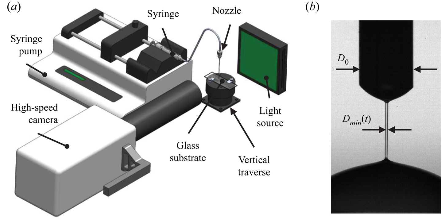
Figure 2. (a) Isometric view of a 3-D model depicting the DoS setup. (b) A sample image taken for PAM with  $c=0.05\,\%$ in elastocapillary thinning.
The pinch-off dynamics of the liquid bridge in the DoS apparatus depends on forces attributed to inertia, surface tension, viscosity and elasticity (Dinic et al. Reference Dinic, Jimenez and Sharma2017). The Ohnesorge number,  $Oh = t_v/t_R$, relates the time scale associated with viscous forces to the Rayleigh time $t_R$, which pertains to surface tension and inertial forces. Here, $t_v = \eta D_0 / 2\sigma$ is the characteristic time scale of viscocapillary thinning, $t_R = (\rho D_0^3/8\sigma )^{1/2}$, and $\sigma$ is the surface tension. Low-viscosity fluids typically have $Oh < 1$ and a necking process dominated by inertial and capillary forces. In this regime, inertiocapillary (IC) thinning is described by a 2/3 power law:
 \begin{equation} \frac{D_{min}(t)}{D_0} = \alpha \left( \frac{t_b-t}{t_R} \right)^{2/3}, \end{equation}
where  $t_b$ is the filament break-up time, and $\alpha$ is a multiplicative pre-factor between 0.4 and 1 (Zhang & Calabrese Reference Zhang and Calabrese2022). If $Oh>1$, viscous forces are significant, and the evolution of $D_{min}$ is described by viscocapillary thinning, $D_{min}(t)/D_0 = 0.0709(t_b-t)/t_v$ (McKinley & Tripathi Reference McKinley and Tripathi2000). For elastic fluids, the Deborah number, $De = t_e / t_R$, describes the ratio of the extensional relaxation time $t_e$ and the Rayleigh time (Tirtaatmadja, McKinley & Cooper-White Reference Tirtaatmadja, McKinley and Cooper-White2006). If $De > 1$, the necking process is dominated by elastic and capillary forces. This elastocapillary (EC) regime is described by
 \begin{equation} \frac{D_{min}(t)}{D_0} = A \exp \left(-\frac{t}{3 t_e} \right), \end{equation}
where  $A = (GD_0/2\sigma )^{1/3}$. The fluids in the present investigation exhibit thinning in an IC ( $Oh<1$) or EC regime ( $De>1$). Nonlinear least-square regression was used to establish $t_e$ for fluids that exhibited EC thinning using measurements of $D_{min}$ and (2.4). Values of $t_e$ are listed in Appendix A.
2.4. Particle shadow velocimetry
Particle image velocimetry (PIV) with backlight illumination, denoted as particle shadow velocimetry (PSV), was used to measure the velocity of the fluid within the test section. In PSV, the thickness of the measurement domain is driven largely by the depth of focus (DOF) of the imaging system. Provided a sufficient magnification and lens aperture, images can be acquired with a thin focal plan that enables 2-D planar flow measurements along a select and narrow region of interest (Santiago et al. Reference Santiago, Wereley, Meinhart, Beebe and Adrian1998; Estevadeordal & Goss Reference Estevadeordal and Goss2006; Khodaparast et al. Reference Khodaparast, Borhani, Tagliabue and Thome2013).
The PSV system consisted of a digital camera (Imager Pro X, LaVision GmbH) with a  $2048 \times 2048$ pixel charged-coupled device sensor. Each pixel was $7.4 \times 7.4$ $\mathrm {\mu }$m $^2$ in size and had a 14-bit digital resolution. A Nikon lens with a focal length of $f=105$ mm was equipped to the camera with an aperture diameter of $f/2.8$. The camera focus was adjusted such that images were focused on the radial mid-span of the test section. Two fields of view (FOVs) were considered, as shown in figure 3(a). The first FOV, i.e. FOV1, considered the entrance or development region immediately upstream of the PCT, as demonstrated in the left-hand side of figure 3(a). The FOV1 captured the complete tube radius, $R_o$, and approximately 3 $\lambda$ along the $x$ direction and immediately upstream of the first oscillation in the PCT. Only the Newtonian flow of water was considered in FOV1. The objective was to determine if the flow entering the PCT was a fully-developed laminar Poiseuille flow. Experimental results for FOV1 are presented separately in Appendix C. The second field of view, FOV2, measured the velocity between the second and fifth oscillation of the PCT, that is, from $x \approx 2\lambda$ to $5\lambda$. For FOV2, flows of the three non-Newtonian fluids through the PCT were measured. Both FOVs were approximately the same size, $(\Delta x, \Delta r) = 3.24 \times 14.1$ mm $^2$, with a scale of 6.88 $\mathrm {\mu }$m pixel $^{-1}$ after the sensor was cropped to remove unnecessary data for $r/R_o>1$. The magnification was 1.07 and the DOF was 87 $\mathrm {\mu }$m, which was approximately 10 % the minimum radius in the PCT, $R_{i}$.

Figure 3. (a) A two-dimensional schematic showing the different PSV fields of view. (b) Sample PSV image (TTAC at  $c = 0.04\,\%$) for FOV2. (c) An enhanced version of the sample image in panel (b) for TTAC at $c=0.04\,\%$ and FOV2.
Backlight illumination of the PIV recordings was achieved using a 15 mJ pulse $^{-1}$ Nd:YAG laser (Solo I-15, New Wave Research Inc.) equipped with a diffuser. A diffuser expanded the laser beam, made the incident light incoherent and changed the wavelength to 610 nm using fluorescent disks. A programmable timing unit (PTU-9, LaVision GmbH) and DaVis 8.4 software (LaVision GmbH) were used to synchronize the camera and laser. Silver coated hollow glass spheres, with diameter $d_p = 10$ $\mathrm {\mu }$m, were used as tracer particles in the flow (S-HGS-10, Dantec Dynamics). These particles were opaque, which was ideal for projecting a shadow on the camera in backlight illumination. The density of the particles, $\rho _p$, was 1400 kg m $^{-3}$. As a result the particle response time, $t_p = \rho _p d_p^2/18 \eta _s$, and particle settling velocity, $u_p = (\rho _p - \rho )d_p^2g/18\eta _s$, could be established. Here, $g$ is the gravitational acceleration. The particle response time, $t_p$, was 7.8 $\mathrm {\mu }$s and the particle settling velocity, $u_p$, was 21.8 $\mathrm {\mu }$m s $^{-1}$. We estimated the Stokes number to be $St = t_p \dot {\gamma }_w$, and the Froude number to be $Fr = 2u_p/U_0$. The largest $St$ was 0.003 and the largest $Fr$ was 0.005, depending on $Q$. Both the Stokes and Froude numbers are small (less than 0.1) and errors attributed to particle inertia and particle settling are negligible.
For FOV1, five sets of measurements were performed for water, each for the different values of  $Q$ listed in § 2.1. The results for FOV1 are presented in Appendix C. The measurements of velocity within the entrance region show good agreement with the theoretical expectations for all values of $Q$, providing good confidence in PSV to produce reasonable measurements. For FOV2, measurements were performed for three different non-Newtonian fluids, each having five different concentrations, and five flow rates $Q$ (75 datasets in total). Additionally, five measurements were performed for distilled water at FOV2 for each value of $Q$. Each dataset consisted of 600 pairs of double-frame images recorded at an acquisition frequency of 7.3 Hz. A sample image of the first frame for TTAC at a mass concentration of 0.04 % is shown in figure 3(b). The time delay, $\Delta t$, between image frames was between 500 and 7000 $\mathrm {\mu }$s depending on the value of $Q$, such that the maximum particle displacement between the image frames was no greater than 15 pixel.
Image processing was performed using DaVis 8.4 software (LaVision Gmbh). First, the images were inverted; the intensity signal at each pixel was subtracted from a constant intensity value. Next, the minimum intensity within each pixel and along the complete image ensemble was determined and subtracted from all images in each dataset. Third, the intensity signals at each pixel were normalized by the average intensity of the ensemble. A sample image (TTAC at a mass concentration of 0.04 %) after performing the previously detailed processing steps can be seen in figure 3(c). Compared to the native image, seen in figure 3(b), the processed image has more clearly defined bright particles for all values of  $r$.
$r$.
Vector fields were established using the ensemble-of-correlation method with an initial interrogation window (IW) size of  $64 \times 64$ pixel ( $0.44 \times 0.44$ mm $^2$ or $0.41R \times 0.41R$) and a final IW size of $16 \times 16$ pixel ( $0.11 \times 0.11$ mm $^2$ or $0.10R \times 0.10R$) with 75 % overlap between neighbouring IWs (Meinhart, Wereley & Santiago Reference Meinhart, Wereley and Santiago2000). The velocity vector was denoted as $\boldsymbol {u}$, with components in cylindrical coordinates being $u_r, u_{\theta },u_x$, corresponding to the velocity along the $r, \theta, x$ directions, respectively. The flow is laminar and steady, with presumably no swirl, i.e. $u_{\theta } = 0$, given the geometric dimensions of the PCT and the Reynolds numbers of the flows in the present investigation (Deiber & Schowalter Reference Deiber and Schowalter1979). We also did not observe evidence of secondary flow re-circulations, turbulence or swirl.
Sources of uncertainty in the PSV measurements were assumed to include: (i) errors due to subpixel interpolation of the correlation function; (ii) the finite DOF; and (iii) optical distortion near the walls of the tube from radial curvature and differences in the refractive index. Each source of uncertainty was conservatively estimated, the details for which are listed below.
(i) Errors from subpixel interpolation are conservatively estimated to be 0.1 pixels according to Raffel et al. (Reference Raffel, Willert, Scarano, Kähler, Wereley and Kompenhans2018). A 0.1 pixel error in displacement translates to an error in velocity of 0.1–1.4 mm s $^{-1}$ depending on $\Delta t$. If this error is normalized by the average centreline velocity, $\langle U_0 \rangle$, the largest velocity error among all flow conditions was 0.012$\langle U_0 \rangle$.
(ii) Quantifying the uncertainties attributed to radial distortion and differences in the refractive index was challenging and would require ray tracing analysis (Minor, Oshkai & Djilali Reference Minor, Oshkai and Djilali2007). Instead, errors from radial distortion were conservatively estimated based on how well the velocity within FOV1 could match the theoretical Poiseuille profile, as discussed in Appendix C. The results of the analysis in Appendix C demonstrated that the largest deviation from the parabolic velocity profile was
$0.04\langle U_0\rangle$.(iii) Slower moving particles within the DOF but outside the centre plane of the tube will bias velocity vectors to lower values. If we consider a parabolic velocity profile when the wall radius
$R_w$ is equal to $R_i$, a DOF that is $0.1R_i$ in thickness would produce a relative error in $u_x$ of approximately $0.003\langle U_0 \rangle$ near the centreline of the PCT and $0.1\langle U_0 \rangle$ near the wall of the PCT. These errors reduce when considering regions of the PCT with a larger wall radius.


The total uncertainty in measurements of  $\boldsymbol {u}$ from PSV was estimated to be the root sum squared value of the three previously listed sources of uncertainty. This was approximately $0.042\langle U_0 \rangle$ near the PCT centreline and $0.108\langle U_0 \rangle$ near the PCT walls, when considering regions of the PCT where $R_w = R_i$. In subsequent plots of velocity within the PCT, error bars are used to display the uncertainty in the velocity measurements from PSV.
2.5. Flow field analysis
The steady flow of complex and Newtonian fluids in the PCT are governed by the following equations for mass and momentum conservation:
 \begin{equation} \left. \begin{array}{c} \displaystyle \boldsymbol{\nabla} \boldsymbol{\cdot} \boldsymbol{u} = 0,\\ \displaystyle \rho \boldsymbol{u} \boldsymbol{\cdot} \boldsymbol{\nabla} \boldsymbol{u} ={-}\boldsymbol{\nabla} p + \boldsymbol{\nabla} \boldsymbol{\cdot} \boldsymbol{\tau}, \end{array}\right\} \end{equation}
where  $p$ is the indeterminate component of the Cauchy stress tensor and $\boldsymbol {\tau }$ is the deviatoric stress tensor. The velocity gradient tensor, $\boldsymbol{\mathsf{L}} = \boldsymbol {\nabla } \boldsymbol {u}$, can be decomposed into the symmetric rate of deformation tensor, $\boldsymbol{\mathsf{D}} = (\boldsymbol{\mathsf{L}} + \boldsymbol{\mathsf{L}}^{{\dagger} })/2$, and anti-symmetric rate of rotation tensor, $\boldsymbol{\mathsf{W}} = (\boldsymbol{\mathsf{L}} - \boldsymbol{\mathsf{L}}^{{\dagger} })/2$, where ${\dagger}$ represents the matrix transpose. The components of $\boldsymbol{\mathsf{D}}$ and $\boldsymbol{\mathsf{W}}$ are listed:
 \begin{gather} \left. \begin{array}{c} \displaystyle {\mathsf{D}}_{rr} = \dfrac{\partial u_r}{\partial r},\quad {\mathsf{D}}_{\theta \theta} = \dfrac{u_r}{r},\quad {\mathsf{D}}_{xx} = \dfrac{\partial u_x}{\partial x},\\ \displaystyle {\mathsf{D}}_{r x} = {\mathsf{D}}_{x r} = \dfrac{1}{2}\left( \dfrac{\partial u_r}{\partial x} + \dfrac{\partial u_x}{\partial r} \right), \end{array}\right\} \end{gather}
 \begin{gather}\omega_{\theta} ={-}2{\mathsf{W}}_{xr} = \frac{\partial u_r}{\partial x} - \frac{\partial u_x}{\partial r}, \end{gather}
where  $\boldsymbol {\omega }$ is the vorticity vector, whose only non-zero component is $\omega _{\theta }$. Undisclosed components of $\boldsymbol{\mathsf{D}}$ and $\boldsymbol{\mathsf{W}}$ are zero. Equation (2.5) reduces to the Navier–Stokes equation for Newtonian fluids when the deviatoric stress tensor is represented by the constitutive equation $\boldsymbol {\tau } = 2\eta _s \boldsymbol{\mathsf{D}}$. For non-Newtonian fluids, the constitutive relation is much more complex and can be a partial differential equation with nonlinear terms (e.g. Phan–Thien–Tanner and Giesekus models). For most non-Newtonian constitutive models, it is common to segregate the deviatoric stress tensor into a solvent and non-Newtonian stress, i.e. $\boldsymbol {\tau } = \boldsymbol {\tau }_{\boldsymbol {s}} + \boldsymbol {\tau }_{\boldsymbol {nn}}$ (Alves, Oliveira & Pinho Reference Alves, Oliveira and Pinho2020). Here, $\boldsymbol {\tau }_{\boldsymbol {s}} = 2\eta _s \boldsymbol{\mathsf{D}}$ is the solvent stress and $\boldsymbol {\tau }_{\boldsymbol {nn}}$ is the non-Newtonian stress introduced from the polymers or micelles. Note that if $\boldsymbol {\tau }_{\boldsymbol {nn}} = 0$, then $\boldsymbol {\tau } = \boldsymbol {\tau _{s}}$ and the constitutive equation is Newtonian. When substituted into (2.5), the divergence of the non-Newtonian stress, $\boldsymbol {\nabla } \boldsymbol {\cdot } \boldsymbol {\tau }_{\boldsymbol {nn}}$, acts as an additional forcing term and for polymeric flows is often referred to as a ‘polymer force’ (Kim et al. Reference Kim, Li, Sureshkumar, Balachandar and Adrian2007).
Equations (2.6) and (2.7) can be explicitly evaluated using the measured  $u_x$ and $u_r$. To circumvent the need for pressure, $p$, we considered the vorticity transport equation obtained from taking the curl of the momentum transport equation, shown in (2.5). The only non-zero component of the vorticity in the PCT flow is $\omega _{\theta }$; therefore, we consider the vorticity transport equation along the azimuthal direction alone:
 \begin{equation} \underbrace{u_r \frac{\partial \omega_{\theta}}{\partial r} + u_x \frac{\partial \omega_{\theta}}{\partial x} - \frac{u_r \omega_{\theta}}{r}}_{VA} = \underbrace{\nu_s \left( \frac{\partial^2 \omega_{\theta}}{\partial r^2} + \frac{1}{r} \frac{\partial \omega_{\theta}}{\partial r} + \frac{\partial^2 \omega_{\theta}}{\partial x^2} - \frac{\omega_{\theta}}{r^2} \right)}_{VSD} + \hspace{0.3em} T_{\theta}. \end{equation}
The additional term on the right-hand side of (2.8), is the azimuthal component of the non-Newtonian torque,  $\boldsymbol {T} = (\boldsymbol {\nabla } \times \boldsymbol {\nabla } \boldsymbol {\cdot } \boldsymbol {\tau }_{\boldsymbol {nn}})/\rho$. The non-Newtonian torque is a vector, whose only non-zero component in the PCT is $T_{\theta }$. Previous numerical investigations have denoted $\boldsymbol {T}$ the ‘polymer torque’ as it can be represented as the curl of the polymer force (Kim et al. Reference Kim, Li, Sureshkumar, Balachandar and Adrian2007, Reference Kim, Adrian, Balachandar and Sureshkumar2008; Kim & Sureshkumar Reference Kim and Sureshkumar2013; Page & Zaki Reference Page and Zaki2015, Reference Page and Zaki2016; Biancofiore, Brandt & Zaki Reference Biancofiore, Brandt and Zaki2017; Lee & Zaki Reference Lee and Zaki2017). Its simplified units are s $^{-2}$ – when multiplied by moment of inertia, the units are force times unit distance, consistent with the true torque definition. The under-braces shown in (2.8) isolate the different combinations of terms within the vorticity transport equation. On the left-hand side of (2.8), $VA$ denotes the azimuthal vorticity advection. The first term on the right-hand side of (2.8), $VSD$, represents vorticity solvent diffusion, where $\nu _s = \eta _s/\rho$. For each flow, the azimuthal non-Newtonian torque was calculated based on the deficit between $VA$ and $VSD$, i.e. $T_{\theta } = VA - VSD$.
To establish the first-order spatial gradients of velocity, a moving second-order polynomial surface was fit on profiles of  $u_x$ and $u_r$. The size of the second-order polynomial filter was $20 \times 20$ pixels, $138\times 138$ $\mathrm {\mu } \textrm {m}^2$ or $0.15R \times 0.15R$. Coefficients of the polynomial surface were used to establish first-order spatial derivatives of $u_x$ and $u_r$. Azimuthal vorticity, $\omega _{\theta }$, was then established using (2.7). To determine the higher order spatial gradients in the flow, a moving third-order polynomial surface was fit on profiles of $u_x$ and $u_r$. The size of the cubic polynomial filter was $76 \times 76$ pixels, $522\times 522$ $\mathrm {\mu } \textrm {m}^2$, or $0.56R \times 0.56R$. Coefficients of the third-order polynomial were used to the determine the second- and third-order spatial derivatives of $u_x$ and $u_r$. Three orders of differentiation in $\boldsymbol {u}$ are required due to the $VSD$ term in (2.8). These higher-order derivatives were then used to calculate the azimuthal non-Newtonian torque $T_{\theta }$ using (2.8). Polynomial filters that overlapped with the PCT wall were neglected, and results of $\omega _{\theta }$ and $T_{\theta }$ were not considered close to the wall.
All parameters including  $\boldsymbol {u}$, $\omega _{\theta }$ and $T_{\theta }$ exhibited symmetry about $r = 0$. Therefore, $\boldsymbol {u}$, $\omega _{\theta }$ and $T_{\theta }$ on the lower half of the domain ( $r<0$) were averaged with the upper half ( $r>0$). When comparing $\boldsymbol {u}$, $\omega _{\theta }$ and $T_{\theta }$ in one oscillation to prior or subsequent oscillations, the parameters are not dramatically different for all flow conditions and fluids. Therefore, $\boldsymbol {u}$, $\omega _{\theta }$ and $T_{\theta }$ were periodically averaged over three oscillations, i.e. for $x$-coordinates that share the same wall radius, $R_w$.
The volumetric flow rate,  $Q$ can be determined from flow measurements based on a volume integration of $u_x$, i.e. $Q = 2 {\rm \pi}\int _{0}^{R_w} u_x r \,\textrm {d}r$. The bulk velocity can be defined according to $U = Q/({\rm \pi} R_w^2)$. Because of mass conservation and the variation of $R_w$ along $x$, the bulk velocity $U$ changes along the streamwise $x$ direction. Therefore, an average value of $U$ along $x$ was determined, and angle brackets $\langle \cdots \rangle$ were used to denote the spatial averaging along the $x$ direction, i.e. $\langle U \rangle$. Recall from § 2.1 that the same angle brackets were used to define the average centreline velocity along $x$,
$x$,  $\langle U_0 \rangle$. An average shape factor can be determined from the ratio of centreline to bulk velocity, $SF = \langle U_0 \rangle / \langle U \rangle$. For Poiseuille flow in a straight-walled tube, $SF=2$. Lastly, distributions of $\boldsymbol {u}$, $\omega _{\theta }$ and $T_{\theta }$ for flows within the PCT (i.e. FOV2) were normalized by $\langle U_0 \rangle$, $\dot {\gamma }_w$ and $\dot {\gamma }_w^2$, respectively. Spatial variables $x$ and $r$ were normalized by $\lambda$ and $R$, respectively. Normalization of the parameters was denoted using the superscript $+$.
$+$.
3. Characterization of fluid rheology
3.1. Shear rheology
Figure 4 displays measurements of  $\eta$ as a function of $\dot {\gamma }$ for the Newtonian and non-Newtonian fluids. Shear viscosity distributions of distilled water are shown in figure 4(a). Measurements of $\eta$ for water are constant with respect to $\dot {\gamma }$ provided $\tau > 2$ mPa and $Ta < 1700$. For $\tau < 2$ mPa, measurements of $\eta$ for water are noisy and scattered. When $Ta>1700$, measurements of $\eta$ for water increase abruptly and are no longer constant with respect to $\dot {\gamma }$; Taylor vortices have corrupted the measurements of $\eta$. The average viscosity of water for $\tau > 2$ mPa and $Ta<1700$ is 0.97 mPa s. This is 3 % lower than the theoretical shear viscosity of water at $20.1\,^{\circ }\mathrm {C}$, 1.00 mPa s.

Figure 4. Steady shear viscosity distributions for (a) the baseline Newtonian fluids, (b) flexible polymer solution PAM, (c) rigid biopolymer solution XG and (d) cationic surfactant solution TTAC. The horizontal black solid line is  $\eta$ for water determined from the empirical correlation of Cheng (Reference Cheng2008). Dashed black lines indicate the lower torque limit ( $\tau < 2$ mPa) and the onset of Taylor vortices ( $Ta>1700$). In panels (b,c), solid coloured lines represent the power-law fits for shear-thinning fluids given by (2.2) and with values provided in Appendix A.
Figure 4(b) shows profiles of  $\eta$ for the five PAM solutions. All five concentrations of PAM exhibit larger values of $\eta$ than water. They also exhibit shear-thinning, where $\eta$ decreases monotonically with increasing $\dot {\gamma }$. At the higher values of $\dot {\gamma }$, $\eta$ appears to increase sharply for $\dot {\gamma }$ with a $Ta$ less than 1700. Nonetheless, the trend by which $\eta$ reduces with respect to $\dot {\gamma }$ is well represented by the power law model (2.2) for measurements with $\dot {\gamma }>0.1$ s $^{-1}$ and $\dot {\gamma } < 100$ s $^{-1}$ – sufficiently below the shear rate that $\eta$ increases abruptly. Values of the consistency, $K$, and flow index, $n$, for PAM are provided in Appendix A.
Figure 4(c) demonstrates profiles of  $\eta$ for the five XG solutions. Similar to PAM, all concentrations of XG exhibit larger values of $\eta$ than water and prevalent shear-thinning. Unlike PAM, $\eta$ appears to increase sharply for $\dot {\gamma }$ with a $Ta$ equal to 1700. The shear-thinning trend is well represented by the power law model (2.2) for measurements with $\dot {\gamma } > 0.1$ s $^{-1}$ and $Ta < 1700$. Values of the consistency, $K$, and flow index, $n$, for XG are provided in Appendix A.
Lastly, figure 4(d) demonstrates shear rheograms for the five TTAC solutions. All five solutions have values of  $\eta$ similar to water (approximately 1.00 mPa s) and independent of $\dot {\gamma }$. A similar water-like shear rheogram was observed by Warwaruk & Ghaemi (Reference Warwaruk and Ghaemi2021) for a 0.015 % and 0.02 % TTAC solution, despite the solutions being able to induce upwards of a 70 % reduction in skin friction drag and attenuate velocity fluctuations in a high-Reynolds-number, turbulent channel flow. Although the solutions have a proclivity to induce complex dynamics in other canonical flows, the TTAC solution does not reflect non-Newtonian features in a steady Couette flow with $\dot {\gamma }$ between 2 and 100 s $^{-1}$.
3.2. Extensional rheology
Measurements of  $D_{min}/D_0$ from the DoS apparatus are shown in figure 5 for the PAM solutions – the only solutions that demonstrated EC thinning. For $t$ less than the inertial break-up time $t_b$, the evolution of $D_{min}$ is in an IC regime and well described by (2.3). The inertial break-up time $t_b$ was not significantly different among the PAM solutions of different $c$ and was approximately $7.2\ \textrm {ms} \pm 0.6\ \textrm {ms}$. Measurements of $D_{min}/D_0$ for PAM with $c = 0.01\,\%$ are shown in the inset axes of figure 5. The IC thinning represented by (2.3), and shown by the black solid line in the inset axes of figure 5, has $\alpha = 0.5$ and $t_R = 1.9$ ms. This value of $\alpha$ is between 0.4 and 1, which is within the margin of experimental expectations (Zhang & Calabrese Reference Zhang and Calabrese2022). The theoretical Rayleigh time $t_R = (\rho D_0^3/8\sigma )^{1/2}$ should be 1.89 ms (assuming $\sigma \approx 72$ mN m $^{-1}$) – not significantly different than $t_R$ derived from fitting (2.3) onto measurements of $D_{\textrm {min}}/D_0$ in the IC regime. Recall that the Ohnesorge number is defined as $Oh = t_v / t_R$, where $t_v = \eta D_0 / 2\sigma$. If $\eta$ in the equation for $t_v$ is taken to be the largest measured viscosity in figure 4 (approximately 0.1 mPa s for PAM with $c = 0.05\,\%$), then $t_v \approx 0.9$ ms and the largest $Oh$ is approximately 0.5.

Figure 5. Normalized minimum filament diameter with respect to time for the PAM solutions, as determined from the DoS system. The inset figure demonstrates a zoomed in distribution along time for PAM with  $c = 0.01\,\%$. Coloured solid lines indicate the fits of the EC regime using (2.4). The solid black line in the inset denotes the fit of the IC regime using (2.3).
For  $t>t_b$, all PAM solutions demonstrate EC thinning, well represented by (2.4) and the coloured lines shown in figure 5. As the concentration grows, the extensional relaxation time $t_e$ increases. Values of $t_e$ are provided in Appendix A. If we assumed that $t_R = 1.89$ ms for all PAM solutions, $De$ was between 1.2 and 25.7 depending on $c$. For the high concentration PAM solutions, the 2 kHz image acquisition rate coupled with the spatial resolution of the camera results in repetitive measurements of $D_{min}/D_0$ over several time instances (i.e. the small horizontal lines).
Solutions of TTAC and XG do not demonstrate EC thinning and therefore,  $De < 1$. A lack of EC thinning is either a result of a low $t_e$ or a large $t_R$, by definition of the Deborah number $De = t_e / t_R$. It is well known that surfactant solutions have a much lower $\sigma$ than the solvent and hence, a large $t_R$ (Zhang et al. Reference Zhang, Schmidt, Talmon and Zakin2005). It is possible that the lack of EC thinning in TTAC could be attributed to low surface tension. Surface tension $\sigma$ is generally 40 % lower for large concentration solutions of cationic surfactants relative to water (i.e. 35–45 mN m $^{-1}$). This would mean that $t_R$ could be approximately 30 % larger for surfactants. We suspect that a 30 % increase in $t_R$ is not sufficient to explain the lack of EC thinning for TTAC. The present investigation does not measure $\sigma$, and hence no definitive conclusion can be made in this regard. However, we suspect that the lack of EC thinning is attributed to low $t_e$ at the conditions imposed by the DoS rheometer. This is another example of how difficult it is to measure $t_e$ using capillary-driven extensional rheometers for drag-reducing surfactant solutions, as previously seen by Warwaruk & Ghaemi (Reference Warwaruk and Ghaemi2021) and Fukushima et al. (Reference Fukushima, Kishi, Suzuki and Hidema2022). It also highlights a need to develop other techniques for measuring extensional features of non-Newtonian solutions, as done by Wunderlich & James (Reference Wunderlich and James1987). Ultimately, PAM solutions have relatively large $t_e$ that could be derived from the DoS rheometer, while TTAC and XG solutions have $t_e$ that could not measured using the DoS apparatus.
4. Flows in the periodically constricted tube
The following section provides the results of the flow measurements within the PCT (i.e. FOV2). Experimental results are presented for different fluids, in the order: (1) water; (2) XG; (3) PAM; and (4) TTAC. Statistics including contours of the velocity magnitude, radial profiles of  $u_x^+$, streamlines and vorticity are provided for the various $Re$ and additive concentrations $c$. The final subsection is dedicated to presenting and comparing the azimuthal non-Newtonian torque $T_{\theta }^+$ of the different non-Newtonian flows within the PCT.
4.1. Newtonian flow
Figure 6 demonstrates contours of the velocity magnitude  $\|\boldsymbol {u}\|^+ = (u_x^2+u_r^2)^{0.5}/ \langle U_0 \rangle$ along with streamlines for the flow of water at five different $Re$ within the PCT. All flows with unique $Re$ have a centreline velocity $U_0$ that attains a maximum value around $x^+ = 0.5$. When $x^+ = 0.5$, the wall radius of the PCT $R_w$ is at its smallest value, $R_w = R_i$. For the lowest $Re$ flow (i.e. $Re = 15.7$), the centreline velocity at $x^+= 0.5$ attains 1.25 $\langle U_0 \rangle$. The lowest magnitude in $U_0$ occurs when $x^+ = 0$ and $1$, and is approximately equal to $0.7\langle U_0 \rangle$ for $Re = 15.7$. At larger $Re$, the centreline velocity at $x^+= 0.5$ is smaller in magnitude – approximately 1.1 $\langle U_0 \rangle$. Values of $U_0$ are also slightly larger for the high- $Re$ cases when $x^+ = 0$ and $1$ compared to the case with $Re = 15.7$ – approximately equal to $0.8\langle U_0 \rangle$. Therefore, when $Re$ increases, the normalized centreline velocity decreases. In all flow conditions, streamlines at large $r^+$ tend to follow the sinusoidal profile of the wall. Near the core, streamlines are more parallel with respect to the streamwise $x$ direction.

Figure 6. Velocity magnitude normalized by the average centreline velocity  $\langle U_0 \rangle$ for different $Re$ of water. Solid black lines overlaid on filled contours are streamlines. The solid black line at the limit of the filled contour is the sinusoidal wall profile.
Profiles of  $u_x^+$ with respect to $r^+$ at different points of $x^+$ are shown in figure 7(a) for water at $Re = 15.7$, $106$ and $203$. Sample error bars are shown for the flow condition with $Re$ of 15.7 and at $x^+ = 0.5$. Relative errors were conservatively estimated to be $0.042\langle U_0 \rangle$ near the centreline of PCT and $0.108\langle U_0 \rangle$ near the wall at $x^+ = 0.5$, as discussed in § 2.4. As noted in the discussion pertaining to figure 6, the low- $Re$ flow of $15.7$ has a large variation in $U_0$. When $x^+ = 0$, $U_0$ becomes $0.75 \langle U_0 \rangle$ and when $x^+ = 0.5,$ $U_0$ equals $1.25 \langle U_0 \rangle$. Newtonian flows with larger $Re$ of 106 and 203 have a centreline velocity of approximately $0.81\langle U_0 \rangle$ when $x^+ = 0$ and $1.1\langle U_0 \rangle$ when $x^+ = 0.5$. Within the PCT contractions and expansions (i.e. $x^+ = 0.25$ and 0.75, respectively), radial profiles of $u_x^+$ are approximately the same. In other words, the velocity is symmetric about $x^+ = 0.5$. Figure 7(b) demonstrates that the streamlines of the Newtonian flows also depend on $Re$. When $Re$ is low, streamlines are more curved and their radial position is closer to the PCT centreline at $x^+ = 0.5$.

Figure 7. (a) Velocity profiles of water at  $Re = 15.7$, 106 and $203$ at different $x$ locations along the PCT. Down sampled error bars are shown for the flow of water at $Re = 15.7$ and $x^+ = 0.5$. (b) Overlaid streamlines of the water flows at different $Re$. The black line in panel (b) indicates the wall profile $R_w$. Symbol colours in panel (a) correspond to the different $Re$ as indicated in panel (b).
As noted with regards to figure 7(a), the velocity in the PCT for water demonstrates a dependence on  $Re$ most notable by the differences in the amplitude of the centreline velocity $U_0$. The standard deviation in the centreline velocity $\mathcal {R}(U_0)$ was computed for each $Re$ and normalized by their respective average centreline velocities $\langle U_0 \rangle$. The normalized standard deviation in $U_0$ is denoted as $\mathcal {R}(U_0)^+ = \mathcal {R}(U_0)/\langle U_0 \rangle$. Values of $\langle U_0 \rangle$ and $\mathcal {R}(U_0)^+$ are listed in table 1 for the different water flows. The inverse proportionality between the amplitude of $U_0$ and $Re$ is clearly demonstrated by the decreasing trend in $\mathcal {R}(U_0)^+$ as $Re$ grows. In addition to centreline velocity, table 1 also lists the average bulk velocity $\langle U \rangle$ and shape factor $SF = \langle U_0 \rangle / \langle U \rangle$ for the flows of water in the PCT. For Newtonian Poiseuille flow in a straight-walled pipe, $SF$ equals 2. Although the PCT is not straight-walled, values of $SF$ for all water flows are approximately 2.1 and not too different from the theoretical $SF$ for straight-walled Poiseuille pipe flow.
Table 1. Bulk and centreline velocity statistics for the flow of water within the PCT at different  $Re$.
$Re$.

Contours of azimuthal vorticity,  $\omega _{\theta }^+$, are shown in figure 8 for water within the PCT. Near the centreline, $\omega _{\theta }^+$ is approximately equal to zero. For all radial and streamwise coordinates, $\omega _{\theta }$ is positive. The maximum $\omega _{\theta }^+$ is situated near the wall and at $x^+ = 0.5$ for all $Re$. Recall from §2.5 that measurements of $\omega _{\theta }^+$ within close proximity (15 % of $R_w$) of the wall were not calculated. This is because the differentiation filter conflicted with the wall.

Figure 8. Vorticity normalized by average wall shear rate  $\dot {\gamma }_w$ for different $Re$ of water. The solid black line is the sinusoidal wall profile.
4.2. Xanthan gum solutions
Velocity contours and streamlines are shown in figure 9 for XG solutions at different  $Re$. For brevity, only the results of two concentrations, $c = 0.02\,\%$ and $0.05\,\%$, are shown. Similar to water, both of the XG solutions with $c = 0.02\,\%$ and $0.05\,\%$ have magnitudes of $\|\boldsymbol {u}\|^+$ that are lowest when $x^+ = 0$ and $1$, and largest when $x^+ =0.5$. Compared to Newtonian water flows seen in figure 6, the zone with larger values of $\|\boldsymbol {u}\|^+$ is extended farther towards the tube wall. As $c$ increases from 0.02 % to 0.05 %, $\|\boldsymbol {u}\|^+$ also increases at $r^+ > 0$ locations. Streamlines at large $r^+$ take on a similar sinusoidal profile as the wall pattern. Similar to the water flows, the streamlines for XG at $c = 0.02\,\%$ and $0.05\,\%$ are approximately symmetric with respect to $x^+ = 0.5$.

Figure 9. Velocity magnitude normalized by the average centreline velocity  $\langle U_0 \rangle$ for different $c$ and $Re$ of XG. Solid black lines overlaid on filled contours are streamlines. The solid black line at the limit of the filled contour is the sinusoidal wall profile.
Streamwise velocity profiles  $u_x^+$ at different $x^+$ coordinates are shown in figure 10(a) for XG with $c = 0.05\,\%$ and at $Re = 10.2$. For comparison, the profiles of water at a similar $Re$ are presented alongside those of XG. Relative to water at the same $x^+$ coordinates, XG has larger $u_x^+$ values. The distributions of $u_x^+$ are more flat in the PCT centre; a blunted profile that is common in shear-thinning fluids (Bird, Stewart & Lightfoot Reference Bird, Stewart and Lightfoot2007). Despite the differently shaped velocity profile, the range of $U_0$ appears to be similar among water and XG. For the XG flow, $U_0 = 0.75\langle U_0 \rangle$ at $x^+ = 0$ and $U_0 = 1.25\langle U_0 \rangle$ at $x^+ = 0.5$ – the same as water. Lastly, figure 10(b) compares the streamlines of the same flows of XG and water seen in figure 10(a). Despite having different velocity profiles with respect to $r^+$, the streamlines for water and XG are approximately the same.

Figure 10. (a) Velocity profiles along different  $x$ locations for XG with $c = 0.05\,\%$ at $Re = 10.2$ and water at $Re = 15.7$. Down sampled error bars are shown for the flow of water at $Re = 15.7$ and $x^+ = 0.5$. (b) Overlaid streamlines of XG and water. The black line in panel (b) indicates the wall profile $R_w$. Red symbols in panle (a) correspond to the water flow with $Re = 15.7$, while blue symbols represent the XG flow with $c = 0.05\,\%$ and $Re = 10.2$.
Based on figure 10(a), it was shown that the shape of  $u_x^+$ profiles with respect to $r^+$ were different, but the relative variations in $U_0$ were the same among the flows of water and XG at similar $Re$. Figure 11(a) demonstrates the standard deviation in $U_0$ normalized by the average centreline velocity, $\mathcal {R}(U_0)^+$, for XG and water. Low-concentration solutions of XG ( $c < 0.03\,\%$) appear to have $\mathcal {R}(U_0)^+$ values that overlap with water at high $Re$. However, for $Re<20$ and high XG concentrations, the values of $\mathcal {R}(U_0)^+$ appear to be independent of the Reynolds number and relatively constant. The higher concentration XG solutions of 0.04 % and 0.05 % appear to have subtly larger values of $\mathcal {R}(U_0)^+$ than water and the other XG solutions; however, the difference is not substantial. Generally, $\mathcal {R}(U_0)^+$ for XG appears to be independent of concentration and similar to water at higher $Re$ values. Figure 11(b) presents the average shape factor $SF = \langle U_0 \rangle /\langle U \rangle$ for water and XG at different $Re$ and $c$ within the PCT. Relative to water, XG flows at all $c$ and $Re$ have lower $SF$ values. As the $c$ of XG increases, $SF$ decreases. The reducing trend in $SF$ aptly summarizes how shear-thinning makes the profile more blunt as the concentration of XG increases.

Figure 11. (a) Standard deviation in the centreline velocity divided by the mean centreline velocity, and (b) the shape factor with respect to different  $Re$ for XG solutions and water.
Vorticity contours for the XG flows with  $c = 0.02\,\%$ and 0.05 % are shown in figure 12. Similar to the flows of water in the PCT, $\omega _{\theta }^+$ attains a maximum value near the wall and at $x^+ = 0.5$. Both the XG flows with $c = 0.02\,\%$ and $0.05\,\%$ have a noticeably attenuated $\omega _{\theta }^+$ in regions farther from the tube centreline. In other words, the thickness (along $r^+$) of the region near the pipe centreline with $\omega _{\theta }^+ = 0$ is larger for XG relative to water. The thickness also grows with increasing $c$. The attenuated $\omega _{\theta }^+$ is attributed to the more uniform profiles of $u_x^+$ caused by shear-thinning.

Figure 12. Vorticity normalized by the average wall shear rate  $\dot {\gamma }_w$ for different $c$ and $Re$ of XG. The solid black line is the sinusoidal wall profile.
4.3. Polyacrylamide solutions
Relative to water and XG, different patterns in the velocity are encountered for the flow of PAM within the PCT. Figure 13 demonstrates contours of  $\|\boldsymbol {u}\|^+$ for PAM at different $c$ and $Re$. In this figure, $c$ increases from bottom to top, and $Re$ increases from left to right. Despite the low- $Re$ flows showing some visual resemblance to the results for water, flows at high $c$ and large $Re$ are asymmetric about $x^+ = 0.5$. For these cases, the large velocity contours take on a triangular or half-chevron appearance leaning towards the upstream direction. Therefore, within the contraction regions (i.e. from $x^+ = 0$ to $0.5$), the maximum velocity is not necessarily situated at the centreline of the PCT. Within the tail of the chevron, streamlines appear to be tilted farther towards the centreline and non-conforming to the sinusoidal profile of the walls. Despite the PAM solutions having seemingly comparable steady shear rheology as the XG solutions (figure 4), the flow of PAM within the PCT produces an entirely different velocity distribution. It is clear that another rheological property, not present in XG, is causing the chevron pattern in the flows of PAM through the PCT.

Figure 13. Velocity magnitude normalized by the average centreline velocity  $\langle U_0 \rangle$ for different $c$ and $Re$ of PAM. Solid black lines overlaid on filled contours are streamlines. The solid black line at the limit of the filled contour is the sinusoidal wall profile.
Streamwise velocity profiles  $u_x^+$ along different $x^+$ values are shown in figure 14(a) for PAM with $c = 0.03\,\%$. Two different $Re$ are compared to contrast the change in the velocity from when the contours transition to the half-chevron seen in figure 13. For the low-Reynolds-number case of $Re = 3.02$ (red symbols), profiles of $u_x^+$ are similar to those for water or XG. The shape of the $u_x^+$ profiles appear to be subtly more blunted than the parabolic Poiseuille profile and the variations in $U_0$ are slightly larger than the values encountered for water at $Re = 15.7$ seen in figure 7(a). Similar to XG, the more blunted velocity profile for PAM at low $Re$ can likely be explained by shear-thinning. Recall that PAM with $c = 0.03\,\%$ has a lower power-law index than XG with $c = 0.05\,\%$, as seen in Appendix A. Therefore, we would expect $u_x^+$ profiles not to be parabolic, but also not as blunted as the higher concentration XG solutions. Although the low- $Re$ flow reflects some similarities to previous findings for XG, the higher $Re$ flow of PAM (blue symbols) exhibits entirely unique distributions in $u_x^+$. At $x^+ = 0$ the $u_x^+$ profile has two local maxima – one at the centreline, the other at $r^+ = 0.9$. Within the contraction, where $x^+ = 0.25$, the maximum value of $u_x^+$ is no longer situated at the centreline, but at $r^+ = 0.6$. Prior works have observed large velocity overshoot near the wall in gradual planar contraction flows of PAM solutions (Poole et al. Reference Poole, Escudier and Oliveira2005) and numerical investigations that used various viscoelastic constitutive models (Afonso & Pinho Reference Afonso and Pinho2006; Alves & Poole Reference Alves and Poole2007; Poole et al. Reference Poole, Escudier, Afonso and Pinho2007; Poole & Alves Reference Poole and Alves2009). Poole et al. (Reference Poole, Escudier and Oliveira2005) referred to these velocity overshoots as ‘cat's ears’ given their appearance.

Figure 14. (a) Velocity profiles along different  $x$ locations for PAM with $c = 0.03\,\%$ at $Re =3.02$ and $Re = 60.5$. Red symbols show $Re = 3.02$ and blue symbols show $Re = 60.5$. Down sampled error bars are shown for the flow of PAM with $c = 0.03\,\%$ and $Re = 3.02$ at $x^+ = 0.5$. (b) Overlaid streamlines of PAM at different $Re$. The black line in panel (b) indicates the wall profile $R_w$.
Coupled with the near-wall velocity overshoots are highly curved streamlines, as shown in figure 14(b). At sufficiently large  $Re$, PAM with $c = 0.03\,\%$ has streamlines that are directed away from the PCT core and more towards the tube wall for $x^+ = 0$ to $0.5$. The works by Cable & Boger (Reference Cable and Boger1978a,Reference Cable and Bogerb, Reference Cable and Boger1979) referred to the state of these curved streamlines as ‘divergent flow’. In general, solutions of PAM with $c \geq 0.02\,\%$ and sufficiently large $Re$ are subjected to near-wall velocity overshoots and divergent flow within the contracting portions of the PCT (i.e. $0< x^+<0.5$), as seen in figure 13.
The pattern of  $u_x^+$ for PAM is clearly dependent on $Re$ and $c$, as observed in figure 13. Compared to water, it can be observed that variations in $U_0$ are larger for PAM at large $c$ and $Re$ based on figure 14(a). Figure 15(a) demonstrates $\mathcal {R}(U_0)^+$ as a function of $Re$ for different $c$ of PAM. When the concentration of PAM is low ( $c = 0.01\,\%$), values of $\mathcal {R}(U_0)^+$ are similar to water. This is expected; contours of velocity for PAM with $c = 0.01\,\%$ do not exhibit a prevalent asymmetric half-chevron pattern in figure 13. At large concentrations, PAM enhances the variations in $U_0$. For more moderate PAM concentrations of $c = 0.02\,\%$ and $0.03\,\%$, $\mathcal {R}(U_0)^+$ increases up until an $Re$ of approximately 35, before decreasing with further growth in $Re$. At large concentrations of $c = 0.04\,\%$ and $0.05\,\%$, values of $\mathcal {R}(U_0)^+$ are similar.

Figure 15. Standard deviation in the centreline velocity divided by the mean centreline velocity with respect to (a) different  $Re$ and (b) different Deborah number $De$ for various PAM solutions.
Rheological measurements of PAM solutions demonstrated that the solutions are viscoelastic – see figure 5 and Appendix B. Therefore, values of  $\mathcal {R}(U_0)^+$ are also contrasted with the elastic properties of the flow. A Deborah number within the PCT was defined as $De = t_e/t_f$, where $t_f = \lambda /\langle U_0 \rangle$ is the time scale of the flow along the PCT centreline. Figure 15(b) shows values of $\mathcal {R}(U_0)^+$ with respect to $De$ for different concentrations of PAM. For all flows of PAM with $c = 0.01\,\%$, the values of $De$ are less than 0.1 and the corresponding values of $\mathcal {R}(U_0)^+$ are less than 0.2. Larger concentration PAM solutions with $De>0.1$ have large values of $\mathcal {R}(U_0)^+$ that are greater than 0.2 and tend to increase with growing $De$ – that is, up until the point where $Re$ has attained 35, with reference to figure 15(a). Based on the trend in $\mathcal {R}(U_0)^+$ versus $Re$ for water, a decreasing $\mathcal {R}(U_0)^+$ is likely attributed to inertial effects – perhaps producing more stagnant flow or small, unseen recirculations in the expansion regions with adverse pressure gradients and where $R_w = R_o$ (Deiber & Schowalter Reference Deiber and Schowalter1981). However, elasticity acts to augment $\mathcal {R}(U_0)^+$. The increasing–decreasing trend in $\mathcal {R}(U_0)^+$ is most likely a result of the competing effects of elasticity and inertia. When $c$ is sufficiently large, elasticity dominates and the trend in $\mathcal {R}(U_0)^+$ as function of $De$ shows better overlap for different $c$. Cases with $De>0.1$ also tend to have a pronounced half-chevron velocity pattern in figure 13.
Lastly, contours of vorticity  $\omega _{\theta }^+$ are shown for the flows of PAM in the PCT in figure 16. At low $c$ and $Re$,
$Re$,  $\omega _{\theta }^+$ is everywhere positive, similar to those for water and XG. However, PAM with sufficiently large $c$ and $Re$ exhibits negative values of $\omega _{\theta }^+$ within the PCT contractions. In certain cases, e.g. $c = 0.03\,\%$ and $Re = 60.5$, there is a strong contrast between the tilted negative contour of $\omega _{\theta }^+$ and the surrounding positive $\omega _{\theta }^+$ values.

Figure 16. Vorticity normalized by  $\dot {\gamma }_w$ for different $c$ and $Re$ of PAM. The solid black line is the sinusoidal wall profile.
4.4. Surfactant solutions
Velocity contours are shown for the TTAC solutions in figure 17. At the lowest concentration of  $c = 0.01\,\%$ and $0.02\,\%$, the contours are similar to those for water. Half-chevron patterns that are similar to the those of PAM appear for all $c$ greater than $0.03\,\%$ and $Re$ that exceed 115. The chevrons result in curved streamlines that are asymmetric with respect to $x^+ = 0.5$. Despite a water-like shear rheogram, shown in figure 4, TTAC demonstrates a complex, non-Newtonian response within the PCT that is similar to flexible polymers and unlike rigid polymers. Therefore, the current measurements show that the rheological trait responsible for the asymmetric chevron pattern in PAM is clearly also inherent in TTAC.

Figure 17. Velocity magnitude normalized by the average centreline velocity  $\langle U_0 \rangle$ for different $c$ and $Re$ of TTAC. Solid black lines overlaid on filled contours are streamlines. The solid black line at the limit of the filled contour is the sinusoidal wall profile.
Profiles of  $u_x^+$ with respect to $r^+$ and at different $x^+$ are shown in figure 18(a) for TTAC with $c = 0.05\,\%$ and $Re = 119$ and compared with PAM at $c = 0.02\,\%$ and $Re = 83.1$ – the closest possible $Re$. The near-wall velocity overshoots encountered for the PAM flows are also present in the TTAC solution. Within the contraction, from $x^+ = 0$ to $0.25$, distributions of $u_x^+$ can be described by a higher-order polynomial with two local peaks along $r^+$. Streamlines are also compared for TTAC and PAM in figure 18(b). Both solutions demonstrate divergent flow patterns within the PCT contraction (Cable & Boger Reference Cable and Boger1978a,Reference Cable and Bogerb, Reference Cable and Boger1979). Streamlines for PAM are projected farther towards the wall relative to TTAC. This is despite PAM having slightly lower near-wall velocity overshoots. In general, we see good qualitative agreement between the velocity field of PAM and TTAC – cat's ears and divergent flow.

Figure 18. (a) Velocity profiles along different  $x$ locations for TTAC with $c = 0.05\,\%$ at $Re = 119$, shown by the red symbols, and PAM with $c = 0.02\,\%$ at $Re = 83.7$, shown with blue symbols. Down sampled error bars are shown for the flow of PAM with $c = 0.02\,\%$ and $Re = 83.7$ at $x^+ = 0.5$. (b) Overlaid streamlines of TTAC and PAM.
Distributions of  $\mathcal {R}(U_0)^+$ as a function of $Re$ are shown in figure 19 for TTAC solutions of different $c$. Solutions that do not exhibit asymmetric velocity patterns, namely TTAC with $c=0.01\,\%$ and $0.02\,\%$, have values of $\mathcal {R}(U_0)^+$ that overlap with those of water and demonstrate the same decreasing trend in $\mathcal {R}(U_0)^+$ with increasing $Re$. For more concentrated solutions of TTAC, such as $c = 0.03\,\%$ and $0.04\,\%$, values of $\mathcal {R}(U_0)^+$ overlap with measurements for water at low $Re$. As $Re$ is increased further, values of $\mathcal {R}(U_0)^+$ abruptly increase. This is different than the monotonic increase in $\mathcal {R}(U_0)^+$ with growing $Re$ observed for PAM in figure 15(a). The $Re$ at which $\mathcal {R}(U_0)^+$ abruptly increases appears to be sensitive to small discrepancies in $Re$. It appears as though transition to large $\mathcal {R}(U_0)^+$ occurs earlier for the $c = 0.04\,\%$ TTAC solution compared to the $c = 0.03\,\%$ solution. However, the $Re$ at which $\mathcal {R}(U_0)^+$ increases for $c = 0.03\,\%$ is subtly larger than the $Re$ of the $c = 0.04\,\%$ solution at a comparable flow rate. Evidently, the resolution of $Re$ is too sparse to capture the sudden augmentation in $\mathcal {R}(U_0)^+$. Ultimately, the trend in the velocity pattern, namely $\mathcal {R}(U_0)^+$ as a function of $Re$, is different for TTAC compared to PAM. Beyond a critical $Re$, the asymmetric velocity patterns that are formed by the TTAC solution exhibit qualitatively the same pattern as PAM, with values of $\mathcal {R}(U_0)^+$ that are also larger than the Newtonian and XG flows.

Figure 19. Standard deviation in the centreline velocity divided by the mean centreline velocity as a function of  $Re$ for the various TTAC solutions.
Figure 20 presents contours of  $\omega _{\theta }^+$ for the TTAC solutions at different $c$ and $Re$. Similar to the PAM solutions, the flows of TTAC with sufficiently large $c$ and $Re$ demonstrate negative values of $\omega _{\theta }^+$ within the contractions of the PCT ( $0< x^+<0.5$). As expected, the conditions where half-chevrons appear in velocity contours also reflect negative values in $\omega _{\theta }^+$. The $c = 0.01\,\%$ and $0.02\,\%$ TTAC solutions have $\omega _{\theta }^+$ distributions that are seemingly identical to those for water, seen in figure 8. At large $c$ and $Re$, negative contours of $\omega _{\theta }^+$ begin to appear. It is notable that the TTAC solutions exhibit water-like rheology, yet they respond in a manner similar to PAM within the PCT at larger $c$ and $Re$ conditions.

Figure 20. Vorticity normalized by  $\dot {\gamma }_w$ for different $c$ and $Re$ of TTAC. The solid black line is the sinusoidal wall profile.
4.5. Non-Newtonian torque
The non-Newtonian torque was established based on the deficit between the advection of vorticity ( $VA$) and the viscous solvent diffusion ( $VSD$) – see (2.8). The normalized azimuthal component of the non-Newtonian torque is $T_{\theta }^+ = T_{\theta }/\dot {\gamma }_w^2$. The distributions of $T_{\theta }^+$ are presented in figures 21, 22 and 23 for water, XG, PAM and TTAC. In these figures, the open contours show $T_{\theta }^+$ and are overlaid on filled contours of $\omega _{\theta }^+$. Contour levels for $T_{\theta }^+$ are from $-$0.4 to $+$0.4 in steps of 0.2. Contours greater than or equal to zero are solid lines and negative contours are dotted lines. Values of $T_{\theta }^+$ were not computed or shown near the wall (within 42 % of $R_w$) due to difficulties in computing spatial gradients within this region, as discussed in § 2.5.

Figure 21. Contours of vorticity and the non-Newtonian torque for the flows of (a) water with  $Re = 106$ and (b) XG at $c = 0.02\,\%$, $Re = 71.7$. Positive and zero contours are solid lines, while dashed lines are negative contours.

Figure 22. Contours of vorticity and the non-Newtonian torque for the flow of PAM solutions with (a)  $c = 0.03\,\%$, $Re = 60.5$ and (b) $c = 0.05\,\%$, $Re = 35.5$. Positive and zero contours are solid lines, while dashed lines are negative contours.

Figure 23. Contours of vorticity and the non-Newtonian torque for the flow of TTAC solutions with (a)  $c = 0.05\,\%$, $Re = 119$, and (b) $c = 0.05\,\%$, $Re = 254$. Positive and zero contours are solid lines, while dashed lines are negative contours.
Based on (2.8),  $T_{\theta }^+$ should be equal to zero in the flow of water. In other words, the dynamics of vorticity should be entirely described by vorticity advection ( $VA$) and diffusion ( $VSD$). Figure 21(a) presents contours of $\omega _{\theta }^+$ and $T_{\theta }^+$ for water at $Re = 170$. Contours of $T_{\theta }^+$ are relatively low in magnitude and noisy. Although XG is a non-Newtonian flow, with evidently large amounts of shear-thinning and linear viscoelasticity (see Appendix B), it too does not have contours of $T_{\theta }^+$ with large magnitude, as seen in figure 21(b). Generally, the plug-like flow of XG within the PCT has a larger region where $\omega _{\theta }^+$ and $T_{\theta }^+$ are equal to 0.
Contours of  $\omega _{\theta }^+$ and $T_{\theta }^+$ for PAM with $c=0.03\,\%$ and $Re = 60.5$ are shown in figure 22(a). A zone of large $T_{\theta }^+$ values is interspersed between regions of negative and positive $\omega _{\theta }^+$ within the PCT contraction. This $T_{\theta }^+$ zone appears in areas where values of $\omega _{\theta }^+$ significantly vary in space. The opposite can be observed within the PCT expansion ( $0.5< x^+<1$); the vorticity reduces with increasing $x^+$, and hence $T_{\theta }^+$ is at its most negative. Similar observations can be made for the flow of PAM with $c = 0.05\,\%$ and $Re = 35.5$ in figure 22(b). Large values of $T_{\theta }^+$ are interspersed between positive and negative contours of $\omega _{\theta }^+$. In both cases, the Newtonian diffusion term ( $VSD$) cannot account for the large spatial variations in $\omega _{\theta }^+$, implying that the non-Newtonian torque is needed to balance the vorticity equation.
Figure 23(a) demonstrates contours of  $\omega _{\theta }^+$ and $T_{\theta }^+$ for TTAC with $c = 0.05\,\%$ at $Re = 119$. Similar to the flows of PAM, TTAC exhibits large values of $T_{\theta }^+$ intermittent between the regions of positive and negative $\omega _{\theta }^+$. The largest positive value of $T_{\theta }^+$ occurs within the contraction, where $\omega _{\theta }^+$ changes abruptly from negative to positive with increasing $x^+$. The same can be observed for larger $Re$ flows, such as TTAC with $c = 0.05\,\%$ and $Re=254$, seen in figure 23(b). As $Re$ increases – comparing figure 23(a,b) – the large positive contour of $T_{\theta }^+ = 0.4$ within the PCT contraction moves closer towards the centreline. Overall, the large values of $T_{\theta }^+$ are coupled with the strong spatial variations in $\omega _{\theta }^+$. Distributions in $T_{\theta }^+$ are relatively consistent among solutions of flexible polymers and surfactants as the two solutions apply the same mechanism via non-Newtonian torque for disrupting $\omega _{\theta }^+$. This mechanism is potentially associated with a common rheological feature that produces the non-Newtonian torque.
5. Discussion
Rheometric measurements showed that PAM and XG have prevalent shear-thinning and linear viscoelasticity, while TTAC has a Newtonian and water-like shear viscosity, as shown in figures 4 and 25 (see Appendix B). However, high  $c$ and $Re$ flows of PAM and TTAC within the PCT demonstrate noticeably similar features. These features include the asymmetric half-chevron velocity pattern, negative vorticity contours and non-Newtonian torque – all of which are not encountered in the flows of water or XG. This peculiar observation in the velocity and vorticity profiles of PAM and TTAC can be explained by non-Newtonian qualities that do not exist for XG. Indeed, XG solutions do not exhibit elastocapillary thinning in DoS rheometry, unlike the PAM solutions shown in figure 5. It is plausible that the chevron-shaped velocity pattern for PAM in the PCT can be explained by a resistance to extensional flow. However, this does not explain the existence of the same chevron-shaped pattern observed for TTAC flows within the PCT since the TTAC solutions do not exhibit elastocapillary thinning. We hypothesize that structures induced by shear, elongational or mixed kinematics are formed within the PCT flow of the surfactant solution when $Re$ is sufficiently large. These structures behave similarly as flexible polymers. The remaining discussion interprets the results for PAM and TTAC further in an attempt to reconcile the cause for their non-Newtonian velocity and vorticity patterns within the PCT.
In viscoelastic flows through gradual planar contractions, large near-wall velocity overshoots have been observed experimentally. Poole et al. (Reference Poole, Escudier and Oliveira2005) were among the first to observe near-wall velocity overshoots in the flow of a PAM solution through a duct that gradually contracted along one Cartesian direction. Poole et al. (Reference Poole, Escudier and Oliveira2005) coined the near-wall velocity overshoot as ‘cat's ears’ due to their appearance. The canonical flow of Poole et al. (Reference Poole, Escudier and Oliveira2005) was not axisymmetric, and later numerical investigations by Afonso & Pinho (Reference Afonso and Pinho2006) and Poole et al. (Reference Poole, Escudier, Afonso and Pinho2007) demonstrated that the magnitude of the velocity overshoot was different depending on the Cartesian plane of interest. Subsequent investigations by Alves & Poole (Reference Alves and Poole2007) and Poole & Alves (Reference Poole and Alves2009) of viscoelastic flows through planar contractions concluded that the cat's ears and divergent streamlines were inherently elastic, and attributed to a large extensional viscosity and first normal stress differences along the centreline of the duct. Velocity statistics for PAM, seen in figures 13 and 14, reflect both cat's ears and divergent flow, implying the PAM solutions impose a large resistance to extensional flow along the centreline of the PCT – as per the conclusions of Alves & Poole (Reference Alves and Poole2007) and Poole & Alves (Reference Poole and Alves2009). Moreover, a complex interplay between elasticity and inertia within the PCT was alluded to, based on the trend in  $\mathcal {R}(U_0)^+$ with respect to $Re$ and $De$ for PAM. From figure 15, it was observed that $\mathcal {R}(U_0)^+$ increased provided $De>0.1$ and $Re<35$. Using these threshold values to delineate the different flow regimes, a qualitative phase diagram shown in figure 24 was constructed. In figure 24, the $De$ and $Re$ of each PAM flow is shown with a colour that corresponds to their respective value of $\mathcal {R}(U_0)^+$. Inset axes in figure 24 show samples of the vorticity field (from figure 16) within each flow regime. The different flow regimes are summarized as follows.

Figure 24. Phase diagram of the different PAM flows in  $De$,
$De$,  $Re$ space. The solid black lines separate the different flow regimes, which are labelled in each quadrant. The four inset axes show sample vorticity contours of flows within each regime. Data point colours correspond to the values of $\mathcal {R}(U_0)^+$ identified from the colour bar.
(i) Inelastic:
$De<0.1$ and $Re<35$. Velocity and vorticity are symmetric with respect to $x^+ = 0.5$, as shown in figures 13 and 16. Velocity contours are similar to those of water or shear-thinning XG solutions. Vorticity is everywhere positive. As $De$ approaches 0.1, $\mathcal {R}(U_0)^+$ is marginally enhanced relative to water flows.(ii) Inertial:
$De<0.1$ and $Re>35$. Mainly distinguished by the decreasing trend in $\mathcal {R}(U_0)^+$ with increasing $Re$ that was similarly observed for water flows in the PCT – seen in table 1 and figures 11(a) and 15(b). Possibly a result of small recirculations or more stagnant flow within the PCT expansion (Deiber & Schowalter Reference Deiber and Schowalter1981; Pilitsis et al. Reference Pilitsis, Souvaliotis and Beris1991).(iii) Elastic:
$De>0.1$ and $Re<35$. Near-wall velocity overshoots are apparent, as shown by figure 14(a). The negative vorticity contours occupy a large region of the PCT contraction. Values of $\mathcal {R}(U_0)^+$ are significantly augmented relative to water and increase further with growing $De$ and $Re$.(iv) Inertioelastic:
$De>0.1$ and $Re>35$. Values of $\mathcal {R}(U_0)^+$ decrease with increasing $Re$; however, near-wall velocity overshoots are present – see figure 18(a). The negative vorticity contour occupies a smaller region of the PCT contraction compared to the elastic flows.


Far more fundamentally interesting is the observation that TTAC solutions also demonstrate cat's ears and divergent flow, as shown in figures 17 and 18, which hints at the their elastic features. Evidently, the PCT stimulates the viscoelastic properties of TTAC through the formation of structures induced from shear, elongation or mixed deformation. The shape of the flow-induced structures are unknown, but they are conjectured to be groupings of micelles that can be conceived as polymer-like aggregates (Rothstein & Mohammadigoushki Reference Rothstein and Mohammadigoushki2020). The sudden jump in  $\mathcal {R}(U_0)^+$ with increasing $Re$, shown in figure 19, demonstrates that these flow-induced structures are formed when $Re$ is greater than 100 within the PCT flows of TTAC. This corresponds to a value of $\dot {\gamma }_w$ of approximately 90 s $^{-1}$. From figure 4(d), no shear-induced structures (SISs) were observed in the shear rheograms of TTAC near 90 s $^{-1}$; however, the PCT undergoes mixed deformations, both shear and extension. An explanation is that extension, or the combination of shear and extension, within the PCT is needed for the formation of these structures – similar to the so called ‘elongation-induced structures’ alluded to by Sachsenheimer et al. (Reference Sachsenheimer, Oelschlaeger, Müller, Küstner, Bindgen and Willenbacher2014), Omidvar et al. (Reference Omidvar, Dalili, Mir and Mohammadigoushki2018) and Recktenwald et al. (Reference Recktenwald, Haward, Shen and Willenbacher2019). It was also observed that extensional DoS rheometry does not demonstrate EC thinning for TTAC, implying these elongation-induced structures are not formed within the filament necking process of the DoS rheometer. The reason extensional DoS rheometry does not reveal these elongation-induced structures for TTAC is either a result of insufficient extensional deformation, or perhaps the lower surface tension of the surfactant solution, which in turn reduces the Rayleigh time $t_R$ and Deborah number $De$ of the necking process. If these structures are shear-induced, perhaps pre-shearing the samples before DoS could enable measurements of $t_e$, similar to prior works such as Wunderlich & James (Reference Wunderlich and James1987), Vissmann & Bewersdorff (Reference Vissmann and Bewersdorff1990), Bhardwaj et al. (Reference Bhardwaj, Richter, Chellamuthu and Rothstein2007) and Fukushima et al. (Reference Fukushima, Kishi, Suzuki and Hidema2022). Regardless of how the structures are formed within the PCT (shear, elongation or mixed kinematics), they produce the same qualitative net-effect as PAM, revealed by the velocity contours of figure 17, and the vorticity and non-Newtonian torque contours of figure 23.
With reference to figure 24, the TTAC flows that exhibit cat's ears fall within the inertioelastic regime, considering their  $Re$ is larger than 35. The similarity between the vorticity patterns for TTAC and PAM, or more precisely the $\mathcal {R}(U_0)^+$ value, can be used to estimate the relaxation time $t_e$ of the TTAC solutions. For example, the TTAC solution shown in figure 20 with $c = 0.05\,\%$ and $Re = 254$ has an $\mathcal {R}(U_0)^+$ value of 0.26, which is equal to the $\mathcal {R}(U_0)^+$ value of the PAM flow with the label A shown in figure 24. Estimating the flow time scale $t_f$ of the TTAC flow based on $t_f = \lambda / \langle U_0 \rangle$ and extracting the $De = 0.12$ from figure 24, the relaxation time of this TTAC solution is estimated to be approximately 4.1 ms. This example shows that measurements of $\mathcal {R}(U_0)^+$ using the PCT along with a phase diagram similar to figure 24 can be used for estimating the relaxation time of the TTAC solutions. However, figure 24 is currently too sparse to provide an accurate map of $\mathcal {R}(U_0)^+$ values. We envisage that a larger and more dense matrix of $\mathcal {R}(U_0)^+$ can be used to obtain an accurate phase diagram for extracting the $De$, and therefore the relaxation time of the TTAC solutions. Ultimately, the PCT is able to uncover the non-Newtonian features of the dilute TTAC solutions.
6. Conclusion
Three non-Newtonian solutions, comprising additives having unique chemical structure, were experimentally investigated in a steady, laminar flow through a periodically constricted tube (PCT). The PCT geometry consisted of an asymmetric tube with a wall radius that was sinusoidal with respect to the streamwise direction. The tube with undulating walls imposed a mixture of shear and extensional deformation, where shear rates were as large as 300 s $^{-1}$ and extensional strain rates as large as 58 s $^{-1}$. The non-Newtonian fluids were aqueous solutions of xanthan gum (XG), polyacrylamide (PAM) and a surfactant referred to as TTAC. The experimental campaign compared several concentrations of each non-Newtonian solution at five unique Reynolds numbers ( $Re$) within the PCT.
Particle shadow velocimetry (PSV) was used to determine the streamwise and radial velocity within the PCT. The vorticity transport equation was used to derive the non-Newtonian contribution to the vorticity field, referred to as the ‘non-Newtonian torque’. Our experimental investigation is the first to produce measurements of the non-Newtonian torque – providing another means for comparison with numerical investigations that can derive the non-Newtonian torque explicitly from constitutive models.
Steady shear rheology demonstrated that both XG and PAM were shear-thinning. PAM solutions were the only non-Newtonian fluids to exhibit elastocapillary thinning from extensional rheology. Within the PCT, solutions of XG demonstrated evidence of a plug-like flow, consistent with expectations for pipe flow of inelastic shear-thinning solutions. PCT flows of PAM solutions exhibited different dynamics depending on the Deborah number ( $De$) and $Re$. A phase diagram that delineated the different flow regimes in $De$–
$De$– $Re$ space was constructed for the PAM solutions, based on the change in the amplitude of the centreline velocity along the streamwise direction of the PCT. Above a $De$ of 0.1, PAM flows within the PCT exhibited ‘chevron’ velocity contours, near-wall velocity overshoots and divergent streamlines with shape and curvature that departed dramatically from the sinusoidal wall profile. Within the contractions of the PCT were regions of negative vorticity and non-Newtonian torque.
The PCT revealed that TTAC solutions have similar non-Newtonian features as PAM solutions when  $Re$ exceeded 100. Unlike PAM solutions, the non-Newtonian features of the TTAC solutions were not detectable from conventional shear and extensional rheometric measurement techniques; TTAC solutions had a shear viscosity that was identical to water and no elastocapillary extensional rheology. Therefore, the measurements using the PCT proved to be a novel technique for uncovering the non-Newtonian features of dilute surfactant solutions. Extension or mixed kinematics within the PCT flows of TTAC promoted the formation of flow-induced structures. It is hypothesized that these structures are long wormlike aggregates of micelles that are analogous to flexible polymers. TTAC solutions that exhibited non-Newtonian features within the PCT reflected qualitative similarities with inertioelastic PAM flows with $De >0.1$ and $Re >35$. A preliminary estimate of the elastic relaxation time of the flow-induced structures was established based on comparisons with PAM flows. However, fine tuning this estimate of the relaxation time requires a denser sweep of $Re$ and $De$ for the PAM flows. Therefore, a well-defined rheological property, such as an elastic relaxation time, has yet to be derived from the PCT flow. If the PCT can provide an estimate for the elastic relaxation time, it is conceivable that the PCT can be used for predicting the drag-reducing capabilities of both flexible polymer and surfactant solutions in a turbulent flow.
Acknowledgements
The authors acknowledge the support of the Natural Sciences and Engineering Research Council of Canada (grant number: RGPIN-2020-07231). The authors also recognize the support of Dr R. S. Sanders for providing access to the torsional rheometer used for measurements of shear viscosity.
Declaration of interests
The authors report no conflict of interest.
Appendix A. Rheological parameters
Values of the consistency  $K$ and flow index $n$ derived from fitting (2.2) onto measurements of $\eta$ for shear-thinning fluids are listed in tables 2 and 3. Table 2 presents the values for PAM solutions, for which the measurements of $\eta$ can be seen in figure 4(b). Table 3 presents the values of $K$ and $n$ for the XG solutions, for which the measurements of $\eta$ can be seen in figure 4(c). For the PAM solutions, measurements of the extensional relaxation time $t_e$ could be determined from DoS rheology and a fit of $D_{min}/D_0$ in the EC regime using (2.4). Values of $t_e$ are listed in table 2 for the PAM solutions of different $c$.
$c$.
Table 2. Rheological parameters of PAM from steady shear rheology and DoS.
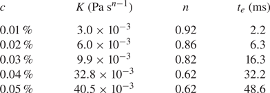
Table 3. Power law model parameters according to (2.2) for XG.

Appendix B. Dynamic shear rheology
Two types of dynamic shear viscosity measurements were performed for each fluid. The first was a stress amplitude sweep,  $\tau _0$, with a constant oscillation frequency, $\omega$, of 0.628 rad s $^{-1}$, or 0.1 Hz. In these tests, $\tau _0$ was increased from 0.2 mPa to 0.3 Pa. Based on the amplitude sweep, the upper limit of $\tau _0$ that corresponds to the linear viscoelastic (LVE) regime was determined (Mezger Reference Mezger2020). Next, a sweep of $\omega$ was performed using a sufficiently small value of $\tau _0$ that is within the LVE regime – for all fluids, a $\tau _0$ of 3.3 mPa satisfied the LVE condition. In the frequency sweep, $\omega$ was varied from 0.1 to 10 rad s $^{-1}$. Trios software (TA Instruments) was used to determine the phase offset, $\delta$, between the applied oscillating stress, $\tau (t)$, and the measured strain, $\gamma (t)$, where $t$ indicates the time dependence of the stress and strain signals. The complex stress modulus was derived from the quotient of the stress and strain amplitudes, $G^* = \tau _0 / \gamma _0$, where $\gamma _0$ is the measured strain amplitude. After determining the complex stress modulus and the phase offset, the storage modulus, $G^{\prime }$, and loss modulus, $G^{\prime \prime }$, could be determined using $G^{*2} = G^{\prime ^2} + G^{\prime \prime ^2}$ and $\tan (\delta ) = G^{\prime \prime }/G^{\prime }$. We present distributions of $G^{\prime }$ and $G^{\prime \prime }$ for the non-Newtonian solutions and comment on the linear viscoelasticity of the fluids.
Unlike steady shear viscosity measurements, dynamic shear viscosity measurements are much more constrained by the torque and inertia limitations of the device – especially when using a single head torsional rheometer (Läuger & Stettin Reference Läuger and Stettin2016). Correcting the torque measurements to compensate for the inertia of the spindle head and geometry can be effective, but not always perfect (Ewoldt et al. Reference Ewoldt, Johnston and Caretta2015; Läuger & Stettin Reference Läuger and Stettin2016). Ewoldt et al. (Reference Ewoldt, Johnston and Caretta2015) recommended ensuring that the torque imposed by the material exceed the torque required to overcome the inertia of the geometry. They derived a limitation on the shear moduli:  $G > IF_{\tau }/F_{\gamma } \omega ^2$, where $G$ can be either $G^{\prime }$ or $G^{\prime \prime }$, and $I$ is the moment of inertia of the geometry. The geometry inertia, $I$, for the rotating inner cylinder was determined to be approximately $4.3\times 10^{-6}$ kg m $^2$. Measurements of $G^{\prime }$ and $G^{\prime \prime }$ that fall below the inertia limitation were disregarded.
Measurements of linear viscoelasticity are shown in figure 25 for high-concentration solutions of PAM and XG. Figure 25(a) demonstrates sweeps of stress amplitudes  $\tau _0$ for PAM solutions, and figure 25(b) demonstrates the same stress amplitude sweep for the XG solutions. Stress amplitude sweeps for PAM with $c = 0.04\,\%$ and $0.05\,\%$, shown in figure 25(a), have $G^{\prime }$ and $G^{\prime \prime }$ values greater than the inertia limit. Lower concentration solutions, with $c \leq 0.03\,\%$, are not shown as their $G^{\prime }$ and $G^{\prime \prime }$ measurements fall below the inertia limit. Both PAM solutions with $c = 0.04\,\%$ and 0.05 % have $G^{\prime \prime } > G^{\prime }$ for all values of $\tau _0$, implying the solutions are viscous dominant when $\omega = 0.628$ rad s $^{-1}$. The difference between $G^{\prime \prime }$ and $G^{\prime }$ diminishes as $c$ increases, i.e. the solution becomes more elastic as $c$ grows. Values of $G^{\prime }$ and $G^{\prime \prime }$ are constant for $\tau _0 < 10^{-2}$ Pa. Therefore, the LVE regime is confined to stress amplitudes less than 10 mPa for PAM. Stress amplitude sweeps for XG solutions, shown in figure 25(b), are similar to PAM. All XG solutions are viscous dominant for $\omega = 0.628$ rad s $^{-1}$. The disparity between $G^{\prime \prime }$ and $G^{\prime }$ decreases as the concentration of XG grows. Values of $G^{\prime }$ and $G^{\prime \prime }$ are constant with respect to $\tau _0$ for $\tau _0 < 4$ mPa.

Figure 25. Dynamic shear viscosity distributions for (a,c) PAM and (b,d) XG. (a,b) Amplitude sweeps at a fixed  $\omega$ of 0.628 rad s $^{-1}$. (c,d) Frequency sweeps at a fixed $\tau _0$ of 3.3 mPa. Hollow symbols are $G^{\prime }$ and filled symbols are $G^{\prime \prime }$. The dashed black line represents the geometric inertia limitation for the measurements Ewoldt et al. (Reference Ewoldt, Johnston and Caretta2015).
Sweeps of  $\omega$ are shown in figure 25(c) for PAM and figure 25(d) for XG. PAM solutions have finite values of $G^{\prime }$ and $G^{\prime \prime }$ for $\omega$ between 0.1 and 10 rad s $^{-1}$. For both $c = 0.04\,\%$ and $0.05\,\%$, the solutions are viscous dominant, $G^{\prime \prime } > G^{\prime }$. As $\omega$ increases, the elastic and viscous moduli become more similar in magnitude, implying the cross-over frequency where $G^{\prime } = G^{\prime \prime }$ is slightly greater than 10 rad s $^{-1}$. Similar to PAM, XG also demonstrates finite $G^{\prime }$ that are lower in magnitude than $G^{\prime \prime }$, i.e. viscous dominant. As $c$ increases, $G^{\prime }$ becomes more similar in magnitude to $G^{\prime \prime }$. Unlike PAM, XG with $c = 0.03\,\%$ and 0.04 % have profiles of $G^{\prime }$ and $G^{\prime \prime }$ that are parallel. In other words, the difference between $G^{\prime }$ and $G^{\prime \prime }$ is not changing with respect to $\omega$. When the concentration is increased to 0.05 %, profiles of $G^{\prime }$ and $G^{\prime \prime }$ appear to begin converging towards one another, implying that the cross-over frequency becomes lower as $c$ increases. Nonetheless, it is likely that the cross-over frequency is well above 10 rad s $^{-1}$ for the XG solutions. Overall, both PAM and XG demonstrate characteristics of uncross-linked polymer solutions with predominantly viscous behaviour. Solutions of TTAC had no measurable $G^{\prime }$ or $G^{\prime \prime }$ values for the same reason the viscous moduli of water could not be measured; dynamic oscillation tests were overcome by the inertia of the geometry for $0.1\ \textrm {s}^{-1}< \omega < 10\ \textrm {s}^{-1}$.
Appendix C. Entrance region
Profiles of streamwise velocity  $u_x$ normalized by the centreline velocity $U_0$ for the flows of water at different $Re_d$ within the entrance region (FOV1) are shown in figure 26(a). Recall that the tube walls have constant radius $R_o$ in the entrance region, and $U_0$ does not vary with respect to $x$. Therefore, the Reynolds number is defined as $Re_d = 2U_0 R_o/\eta _s$. Shown alongside the measurements of $u_x^+$ is the theoretical Poiseuille velocity profile for laminar pipe flow of a Newtonian fluid within a straight-walled pipe, $u_x^+ = 1-r^2/R_o^2$. All measurements of $u_x^+$ are within 4 % of the theoretical Poiseuille profile for different coordinates of $r^+$ and agree well with theoretical expectations. Profiles of the shear component of the rate of deformation tensor ${\mathsf{D}}_{rx}$ are shown in figure 26(b). When the Poiseuille profile for Newtonian pipe flow is differentiated, the relationship $\partial u_x/\partial r = 2{\mathsf{D}}_{rx} = -2U_0 r/R_o^2$ is obtained. When simplified, it can be shown that ${\mathsf{D}}_{rx}R_o/U_0 = -r/R_o$. Similar to the streamwise velocity profiles, measurements of ${\mathsf{D}}_{rx}R_o/U_0$ agree well with the theoretical profile for all $Re_d$. In general, figure 26 demonstrates that measurements within the entrance region reasonably satisfy the expectations for laminar fully-developed Newtonian pipe flow. We can proceed to measurements of the PCT knowing that the flow entering the PCT section is fully developed and the measurement technique is valid.

Figure 26. Radial profiles of (a) streamwise velocity and (b) the shear rate, at FOV1 for the flow of water at various  $Re_d$. Error bars are shown for $Re = 13.2$ and correspond to the $0.042\langle U_0 \rangle$ uncertainty assumed from § 2.4.


 Open access