


1. Introduction
Cavitation commonly occurs on marine lifting surfaces, such as propellers, hydrofoils, turbines, and energy harvesting and energy saving devices during high-speed operation near the free surface. Cavitation occurs when the absolute local fluid pressure drops to the saturated vapour pressure, which leads to the formation of vapour bubbles. When the local pressure falls below the saturated vapour pressure, the fluid is subject to tension at the magnitude of the difference between the local pressure and saturated fluid pressure. When the tension is greater than the tensile strength of the fluid, the fluid ruptures and a cavity is formed (Brennen Reference Brennen1995). The interface between the fluid and body also contains voids that can serve as a rupture point for bubbles to grow. This formation of rupture, as well as rupture around a solid contaminant particle in the fluid, is known as heterogeneous nucleation (Brennen Reference Brennen1995). Rupture can also occur when there is a void in the fluid, which is known as homogeneous nucleation (Brennen Reference Brennen1995). A similar but different phenomenon is ventilation, during which cavities filled with a non-condensible gas are entrained from a nearby free surface (atmospheric ventilation) or injected by force (forced or artificial ventilation) (Acosta Reference Acosta1973; Faltinsen Reference Faltinsen2005; Young et al. Reference Young, Harwood, Montero, Ward and Ceccio2017). Although there is much similarity between cavitation and ventilation, the formation and collapse mechanisms are different between the two phenomena owing to the differences in condensibility and compressibility of the vapour versus gas within the cavities. This paper focuses primarily on vaporous cavitation.
Vaporous cavitation on the body can be categorized as bubbly cavitation, partial cavitation or supercavitation. Bubbly cavitation occurs during the initial stages of cavitation, during which individual bubbles form in the low-pressure region of the suction side of the body and travel downstream, where they collapse as the local pressure increases. Partial cavitation occurs when the cavity collapses onto the body surface, while supercavitation occurs when the cavity collapses aft of the body. Vaporous cavitation can also be categorized by their form, including sheet cavitation and cloud cavitation. Sheet cavitation occurs when the the separated flow region is filled with vapour, and the cavities remain attached to the body, giving a sheet like appearance. Cloud cavitation occurs when there is unsteady or periodic formation, detachment and collapse of sheet cavities, giving the cavitation a cloud like appearance (Brandner et al. Reference Brandner, Walker, Niekamp and Anderson2010). Cavitation can lead to reduction in lift and thrust, increase in drag, strong vibrations, noise and material damage. Cloud cavitation can cause heavy periodic damage with maximum pressures of the order of 133 bar, as the series of collapsing cavities create energy that propagates towards the centre of the cluster, which can lead to greater damage (van Terwisga et al. Reference van Terwisga, Fitzsimmon, Li and Foeth2009). The collapse of cloud cavitation results in erosion pitting, during which material on the surface of the lifting body is removed (Franc et al. Reference Franc, Riondet, Karimi and Chahine2012). Cavitation damage can be especially harmful to composite marine lifting surfaces. Hammond, Amateau & Queeny (Reference Hammond, Amateau and Queeny1993) compared the cavitation damage of several composites (E-Glass/5920, AS4/APC-2, IM7/977-2 T and Scotch Ply 1002) with that of a nickel aluminium bronze (NAB) specimen, and found that all composites sustained higher cavitation erosion damage compared with the NAB specimen. Over time, cavitation can strongly degrade maritime operation performance.
Shedding from cloud cavitation can be driven by Kelvin–Helmholtz wave instabilities, the formation of the re-entrant jet and the shock-wave mechanism. Kelvin–Helmholtz instabilities occur at the interface of two streams of fluid travelling at different velocities. Any small disturbance of the interface results in a wave reaction, which can encourage the shedding of cavities (Brandner et al. Reference Brandner, Walker, Niekamp and Anderson2010). The re-entrant jet phenomenon leads to cavity shedding commonly known as Type II oscillations (Kawanami et al. Reference Kawanami, Kato, Yamaguchi, Tanimura and Tagaya1997; De Lange & De Bruin Reference De Lange and De Bruin1998; Pham, Larrarte & Fruman Reference Pham, Larrarte and Fruman1999). The re-entrant jet is a liquid flow driven by the adverse pressure gradient from the cavity trailing edge to upstream underneath the attached cavity on the body surface (Kawanami et al. Reference Kawanami, Kato, Yamaguchi, Tanimura and Tagaya1997). The jet pinches the sheet cavity interface near the leading edge, which allows cavities to detach and travel downstream to form a cloud-like appearance (Pham et al. Reference Pham, Larrarte and Fruman1999). The Strouhal number of re-entrant jet cavity shedding, which is dependent on the maximum cavity length, lies constant at approximately 0.2 to 0.4 for different hydrofoil geometries and test conditions (Callenaere et al. Reference Callenaere, Franc, Michel and Riondet2001). As such, the cavity shedding frequency is dependent on the maximum cavity length, which in turn is dependent on cavitation number and effective angle of incidence. However, it is important to recognize that this only estimates the dominant cavity shedding frequency. The actual frequency response may contain other frequencies, as the cavities tend to shed in multiple small clouds and the cavity length is typically not uniform along the span of the body owing to three-dimensional (3-D) effects. After the collapse of cavities, remnant micro-bubbles remain and can be carried upstream in the re-entrant jet owing to the high adverse pressure, which serve as re-nucleation sites for the development of new attached cavities (Barbaca et al. Reference Barbaca, Venning, Russell, Russell, Pearce and Brandner2020; Ram, Agrawal & Katz Reference Ram, Agrawal and Katz2020; Russell & Brandner Reference Russell and Brandner2021). The leading edge cavity grows to the maximum cavity length to repeat the process of re-entrant jet formation and cavity shedding.
As the cavitation number decreases, the cloud cavitation length grows toward the trailing edge and the re-entrant jet loses the ability to pinch off cavities owing to a loss of momentum while travelling towards the leading edge (Bhatt et al. Reference Bhatt, Wu, Ganesh and Ceccio2018). This usually occurs when the maximum cavity length is larger than approximately 75 % of the chord length (Fujii et al. Reference Fujii, Kawakami, Tsujimoto and Arndt2007). The cavity shedding mechanism transforms to a shock-wave-induced mechanism, known as Type I oscillations. A shock occurs when the local speed of sound drops below the flow speed of the bubbly mixture in the cavity (Ganesh, Mäkiharju & Ceccio Reference Ganesh, Mäkiharju and Ceccio2016). Although the speed of sound is approximately  $1500\,\textrm {m}\,\textrm {s}^{-1}$ in water, it varies significantly with local void fraction, or the fraction of gas and vapour in a given volume. In vaporous cavitation, the vapour volume fraction varies between 0 and 1. The speed of sound can drop drastically owing to high compressibility and density variation, including to levels of approximately $6\,\textrm {m}\,\textrm {s}^{-1}$ at void fractions between 50 % and 60 %; at higher void fractions, the speed of sound rises to its speed of gas, near $350\,\textrm {m}\,\textrm {s}^{-1}$ (Shamsborhan et al. Reference Shamsborhan, Coutier-Delgosha, Caignaert and Nour2010). A shock condensation front develops at the trailing edge of the cavity and moves upstream towards the leading edge, pinching off cavities, which result in strong periodic shedding clouds (Ganesh et al. Reference Ganesh, Mäkiharju and Ceccio2016; Wu, Maheux & Chahine Reference Wu, Maheux and Chahine2017; Bhatt et al. Reference Bhatt, Wu, Ganesh and Ceccio2018). Shock-wave-based shedding is governed by the change in the local speed of sound of the fluid mixture, and usually occurs at a constant frequency of 10–12 Hz regardless of geometry or facility (Fujii et al. Reference Fujii, Kawakami, Tsujimoto and Arndt2007; Ganesh et al. Reference Ganesh, Mäkiharju and Ceccio2016; Bhatt et al. Reference Bhatt, Wu, Ganesh and Ceccio2018; Smith et al. Reference Smith, Venning, Pearce, Young and Brandner2020a,Reference Smith, Venning, Pearce, Young and Brandnerb). It has also recently been shown that re-entrant jet shedding and shock-wave shedding can occur simultaneously, and has been recorded to occur when the cavity length to chord length ratio, $L_c/c$, is between 1 and 1.25 (Smith et al. Reference Smith, Venning, Pearce, Young and Brandner2020a,Reference Smith, Venning, Pearce, Young and Brandnerb). The two shedding mechanisms can also occur simultaneously as a coupled mechanism in bluff-body flow about a sphere (de Graaf, Brandner & Pearce Reference de Graaf, Brandner and Pearce2017).
Many structures are deformable owing to flexibility of the material or connections. In response to fluid flow, deformable structures may bend and twist. The resulting deformation can interact with fluid flow, and this is known as fluid–structure interaction (FSI). FSI can lead to flow-induced vibrations, which can cause dynamic load oscillations, vibrations, noise and accelerated fatigue. Hydrodynamic instabilities such as divergence (unbounded deformation until material failure develops owing to fluid disturbing forces/moments equal to or exceeding elastic restoring forces/moments), flutter (sustained or growing oscillations owing to zero or negative damping) (Chae, Akcabay & Young Reference Chae, Akcabay and Young2013; Chae et al. Reference Chae, Akcabay, Lelong, Astolfi and Young2016; Chae, Akcabay & Young Reference Chae, Akcabay and Young2017; Harwood et al. Reference Harwood, Felli, Falchi, Ceccio and Young2019) and parametric resonance (exponential growth in vibrations caused by the periodic fluid force modulation at two times the system resonance frequency) (Akcabay & Young Reference Akcabay and Young2015) may develop. While flow-induced vibrations and associated dynamic load amplifications are unwanted for most lift-generating devices, it can be used to harvest flow kinetic energy. Sample studies exploring the energy harvesting potential of flexible piezoelectric plates in air and in water can be found in Akcabay & Young (Reference Akcabay and Young2012) and Wang et al. (Reference Wang, Alben, Li and Young2016). A better understanding of the FSI can also lead to design optimization, as the load-dependent anisotropic deformations can be tailored to delay flow separation, stall, cavitation, static divergence and avoid material failure (Young et al. Reference Young, Harwood, Montero, Ward and Ceccio2017; Liao, Martins & Young Reference Liao, Martins and Young2019). The FSI has also facilitated the development of flow and structural health monitoring techniques with embedded strain gauging or fibre optic techniques (Rajan & Prusty Reference Rajan and Prusty2017; Ward, Harwood & Young Reference Ward, Harwood and Young2018; Di Napoli et al. Reference Di Napoli, Young, Ceccio and Harwood2019). This is especially relevant with the movement towards autonomous marine operations.
The fluid–structure interaction in multiphase flow is currently not well understood. In cavitation and ventilation, the FSI response and stability are difficult to predict. The fluid forces (with fluid inertia, damping and disturbing/restoring force terms proportional to the acceleration, velocity and displacement, respectively, as well as cavity excitation forces caused by unsteady cavity shedding) can all change with the cavitation and ventilation. Because the water and vapour densities are different by five orders of magnitude, the fluid forcing terms are directly impacted and are time dependent in unsteady cavitating and ventilating flows (Akcabay & Young Reference Akcabay and Young2015; Harwood et al. Reference Harwood, Felli, Falchi, Garg, Ceccio and Young2020). The periodic changes in fluid forces caused by cavity shedding and fluctuating fluid-mixture density can induce parametric excitation of the hydrofoil (Chae et al. Reference Chae, Akcabay and Young2013; Akcabay & Young Reference Akcabay and Young2015; Chae et al. Reference Chae, Akcabay, Lelong, Astolfi and Young2016, Reference Chae, Akcabay and Young2017). There has been very little work on the quantification of the effects of cavitation and ventilation on the fluid forces. Fluid added mass in fully ventilated and partially cavitating regimes is generally lower than that in a fully wetted regime owing to a drop in the local fluid density (Akcabay & Young Reference Akcabay and Young2015; Harwood et al. Reference Harwood, Felli, Falchi, Garg, Ceccio and Young2020). Through empirical mode decomposition, it has also been shown that oscillating cavity length along the fluid–structure interface can cause fluctuations in the added mass (Rajaomazava et al. Reference Rajaomazava, Benaouicha, Astolfi and Boudraa2021). The system natural frequency is dependent on the fluid added mass, so system natural frequencies are also altered in multiphase flows (De La Torre et al. Reference De La Torre, Escaler, Egusquiza and Farhat2013; Harwood et al. Reference Harwood, Felli, Falchi, Garg, Ceccio and Young2020; Young et al. Reference Young, Wright, Yoon and Harwood2020). The bandwidth of the system mode frequency tends to increase owing to a decrease in the added mass (Lelong, Guiffant & André Astolfi Reference Lelong, Guiffant and André Astolfi2017). There are many sources of damping, such as radiation, viscous, wake and cavity damping, so the change in damping is generally nonlinear and dependent on the mode of motion and extent of cavitation or ventilation (Harwood et al. Reference Harwood, Felli, Falchi, Garg, Ceccio and Young2020). Generally, damping increases with the submergence of the hydrofoil and with increasing forward speed. Hydrodynamic damping is typically much higher than structural damping, particularly for the lower-ordered modes (Blake & Maga Reference Blake and Maga1975; Chae et al. Reference Chae, Akcabay and Young2017; Harwood et al. Reference Harwood, Felli, Falchi, Garg, Ceccio and Young2020). The rate of change of the fluid density also induces added damping on the structure (Rajaomazava et al. Reference Rajaomazava, Benaouicha, Astolfi and Boudraa2021). Moreover, both the fluid added mass and damping depend on the direction of motion, i.e. mode dependent. Although there has been some qualitative work completed, very little work has been done to quantify how the fluid inertial, damping and disturbing forces change with flow conditions, such as speed, angle of incidence and multiphase flow. The cavity shedding frequency during cloud cavitation can also be affected by the FSI. As reviewed above, the frequency of Type II cavity shedding is a function of the cavity length. Deformable hydrofoils with nose-up bend–twist coupling showed an increased cavity length, which reduced the Type II cavity shedding frequency (Pearce et al. Reference Pearce, Brandner, Garg, Young, Phillips and Clarke2017; Young et al. Reference Young, Garg, Brandner, Pearce, Butler, Clarke and Phillips2018; Smith et al. Reference Smith, Venning, Pearce, Young and Brandner2020b). Hence, the presence of ventilation or cavitation can lead to very different dynamic responses from fully wetted flow (Young et al. Reference Young, Wright, Yoon and Harwood2020).
Another interesting FSI phenomenon involving unsteady cavitating flow is lock-in, which occurs when one of the cavity shedding frequencies is close to one of the system natural frequencies (primary lock-in), its harmonics (super-harmonic lock-in) or subharmonics (subharmonic lock-in). When lock-in occurs, the cavity shedding frequency deviates from the trend typically observed for rigid hydrofoils, such as constant Strouhal number based on cavity length for Type II re-entrant jet shedding, and synchronizes with the adjacent system natural frequency, harmonic or subharmonic, causing an amplification in the system response (Kato, Dan & Matsudaira Reference Kato, Dan and Matsudaira2006; Ausoni et al. Reference Ausoni, Farhat, Escaler, Egusquiza and Avellan2007; Akcabay et al. Reference Akcabay, Chae, Young, Ducoin and Astolfi2014a; Young et al. Reference Young, Harwood, Montero, Ward and Ceccio2017; Náprstek & Fishcer Reference Náprstek and Fishcer2019). The system natural frequency or harmonic may also deviate slightly towards the cavity shedding frequency during lock-in (Lelong et al. Reference Lelong, Guiffant and André Astolfi2017). Super-harmonic and subharmonic lock-ins are heavily reliant on the form of the damping (which is usually nonlinear) as well as the specific damping parameters. Systems with high damping have a wider zone of lock-in, which means that the cavity shedding frequency can be farther away from the subharmonic of the system natural frequency, and lock-in will still occur, but the dynamic load amplification tends to be limited owing to the high hydrodynamic damping. In general, the zone of resonance for subharmonic lock-in is greater than that for super-harmonic lock-in (Náprstek & Fishcer Reference Náprstek and Fishcer2019). Fluctuating hydrodynamic forces may also excite resonant frequencies, which leads to dynamic load amplification for cases with low damping (Ducoin, Astolfi & Sigrist Reference Ducoin, Astolfi and Sigrist2012; Harwood et al. Reference Harwood, Felli, Falchi, Ceccio and Young2019). Unsteady cavity shedding also leads to frequency modulation, which results in a more broad-banded frequency response spectrum (Harwood et al. Reference Harwood, Felli, Falchi, Ceccio and Young2019).
Another FSI phenomenon that is possible in unsteady cavitating flow is the development of heterodyne frequencies. Heterodyne frequencies are generated as the sum and difference of two frequencies when they are input into an oscillating system. The generation and application of heterodyne frequencies are studied in fields such as sonochemistry (Reno, Korremula & Casadonte Reference Reno, Korremula and Casadonte2019), defect detection (Tashakor et al. Reference Tashakor, Baghalian, Senyurek, Unal, McDaniel and Tansei2018) and radio transmission (Weng, Lin & Way Reference Weng, Lin and Way2008). However, heterodyne frequencies generated by the mixing of two cavity shedding mechanisms (i.e. re-entrant jet-driven and shock-wave-driven cavity shedding), where the local fluid medium and/or the flexible hydrofoil can act as a nonlinear oscillator/mixer, have not been discussed in the previous literature. Such an effect is important, as the heterodyne frequencies change the frequency spectra of the response, which can be important for identification of cavitation phenomena, and for prediction of cavity-induced vibrations, load oscillations, accelerated fatigue and potential instabilities.
Owing to the computational cost of performing computational fluid dynamics and/or computational structure dynamics (CFD/CSD) techniques, and the compatibility of control law design with reduced-order models (ROMs), there has been an increase in the modelling of unsteady flows with ROMs. ROMs are useful not only to predict, explain and control responses, but they can also be used to determine scaling relations and identify when lock-in or instabilities may develop.
Gao et al. (Reference Gao, Zhang, Kou, Liu and Ye2017) presented a linear ROM to model the unsteady flow interactions of transonic buffet flow. The ROM was developed through recording the output (lift and moment coefficient) signal induced by a chirp input (airfoil flap angle) signal obtained through CFD, developing a linear model using the input and output signal through system identification, and then reducing the order of the model through a balanced truncation method. The outputs of a linear ROM modelling transonic buffet flow over a NACA0012 airfoil were compared with the outputs of a full-order model from CFD/CSD simulation by Gao, Zhang & Li (Reference Gao, Zhang and Li2019), and it was found that the outputs of the ROM compared well with those of the full-order models. An additional advantage of using ROMs is that the coupled patterns between the fluid mode and structural mode in unsteady flow can be clearly captured (Gao & Zhang Reference Gao and Zhang2020). Other studies of ROMs on unsteady flow include the development of ROMs for the analysis of vortex-induced vibrations about a long flexible cylinder in both the in-line and cross-flow directions. A forced van der Pol oscillator was used along the cross-flow direction and a linear state space model was used in the inflow direction, the results of which were validated with experimental data from a wave tank (Stabile, Matthies & Borri Reference Stabile, Matthies and Borri2018). A simplified ROM based on the van der Pol equation was also proposed to model turbulent flow around a NACA0015 airfoil, the results of which compared well with high-fidelity simulation results (Siddiqui, Rasheed & Kvamsdal Reference Siddiqui, Rasheed and Kvamsdal2020).
While much work can be found on the development of ROMs for single-phase flows, much less work can be found on the development of ROMs for cavitating flows. Simulation of unsteady cavitating flow using CFD is expensive, particularly if the effects of viscosity, turbulence and compressibility all need to be considered in addition to phase change to simulate both re-entrant jet and shock-wave-driven cavity shedding mechanisms. The problem becomes even more complicated when the FSI effects are important. Hence, it is important to develop and validate a ROM based on the physics of experimental data to predict and control unsteady cavitation on flexible lifting surfaces.
Akcabay & Young (Reference Akcabay and Young2015) developed a simple ROM to predict the effects of parametric excitations of flexible hydrofoils in unsteady cavitating flow. The model was developed using data from two sets of experiments of cavity-induced vibrations of cantilevered hydrofoils in the high-speed cavitation tunnel at the French Naval Academy (Ducoin et al. Reference Ducoin, Astolfi and Sigrist2012; Akcabay et al. Reference Akcabay, Young, Lelong and Astolfi2014b; Chae et al. Reference Chae, Akcabay, Lelong, Astolfi and Young2016). Ducoin et al. (Reference Ducoin, Astolfi and Sigrist2012) performed the experiment on a NACA66-213 hydrofoil made of a polyoxymethylene (POM) polyacetate, while Akcabay et al. (Reference Akcabay, Young, Lelong and Astolfi2014b) and Chae et al. (Reference Chae, Akcabay, Lelong, Astolfi and Young2016) presented experimental and numerical data on a NACA0015 hydrofoil made of the same POM polyacetate. Using a simplified one-degree-of-freedom (1-DOF) model for spanwise bending coupled with a van der Pol model capturing the unsteady Type II re-entrant jet cavity excitation forces with the foil bending vibrations, the ROM modelled the frequency response of flexible hydrofoils. The estimations from the ROM were compared with experimental results from Ducoin et al. (Reference Ducoin, Astolfi and Sigrist2012), Akcabay et al. (Reference Akcabay, Young, Lelong and Astolfi2014b) and Chae et al. (Reference Chae, Akcabay, Lelong, Astolfi and Young2016). It was shown that the ROM could accurately predict the primary frequency response, including primary lock-in and modulations. However, the ROM was limited in that it only considered the Type II re-entrant jet cavity shedding frequency but not the Type I shock-wave-driven cavity shedding frequency, and could not predict subharmonic excitations. Moreover, while the predicted frequency response matched well with the measurements, there were large deviations in the amplitude of the oscillations.
In Alavi, Haddadpour & Firouz-Abadi (Reference Alavi, Haddadpour and Firouz-Abadi2018b), a ROM was developed for hydroelastic analysis of a hydrofoil in partial sheet cavitation by first assuming constant cavity length and then imposing velocity perturbation terms to model the unsteady flow. The unsteady hydrodynamic terms were approximated through a finite element solution. The ROM could accurately model cavity length as a function of cavitation number, variations in damping and frequency of different hydrodynamic modes, and flutter speed with and without the presence of cavities. The ROM was used to model the hydroelastic analysis of supercavitation effects in Alavi, Haddadpour & Firouz-Abadi (Reference Alavi, Haddadpour and Firouz-Abadi2018a), where steady pressure distribution and ROM were used to predict flutter velocity. However, there was little discussion in these two works regarding the modelling of cloud cavitation.
Smith et al. (Reference Smith, Venning, Pearce, Young and Brandner2020a) (Part I) and Smith et al. (Reference Smith, Venning, Pearce, Young and Brandner2020b) (Part II) discussed the FSI of a stiff hydrofoil manufactured from Type 316 stainless steel (SS) and a flexible hydrofoil manufactured from a carbon/glass-epoxy composite (CF) structure, respectively. Part II (Smith et al. Reference Smith, Venning, Pearce, Young and Brandner2020b) also compared the FSI of the two hydrofoils. Both hydrofoils experienced cloud cavitation and supercavitation, and the SS hydrofoil experienced sheet cavitation at higher cavitation numbers. It was found that at higher cavitation numbers, the CF hydrofoil experienced a higher ratio of cavity length,  $ {L_{c}}$, over the local chord, $ {c}$, owing to a nose-up twist. This caused an early transformation from the sheet cavitation regime to the cloud cavitation regime, longer cavity and a reduced Type II cavity shedding frequency. Similar observations were made by Young et al. (Reference Young, Harwood, Montero, Ward and Ceccio2017). In addition, multiple lock-in modes occurred at different cavity shedding frequencies on the CF hydrofoil, whereas fewer lock-in modes occurred on the SS hydrofoil. Similar observations were made by Pearce et al. (Reference Pearce, Brandner, Garg, Young, Phillips and Clarke2017) and Young et al. (Reference Young, Garg, Brandner, Pearce, Butler, Clarke and Phillips2018). Lock-ins were frequently observed at subharmonic frequencies of the wetted natural frequencies of the CF hydrofoil. This is supported by findings by Akcabay et al. (Reference Akcabay, Chae, Young, Ducoin and Astolfi2014a). The cavity and the response of the CF hydrofoil became much more stable once the supercavitation regime was achieved. This result was also predicted through numerical methods (Akcabay & Young Reference Akcabay and Young2014, Reference Akcabay and Young2015).
1.1. Objectives
Although much work has been done, the FSI of flexible hydrofoils in cloud cavitation is still not well understood and the dynamic response is not well predicted. Complementing the experimental results presented in Parts I and II (Smith et al. Reference Smith, Venning, Pearce, Young and Brandner2020a,Reference Smith, Venning, Pearce, Young and Brandnerb), this paper aims to further examine the experimental measurements, develop and use ROM predictions to explain the complex FSI response. The novel contributions include: (1) developing and validating ROMs to predict and explain the steady-state and dynamic hydroelastic response of hydrofoils in cloud cavitation; (2) quantifying the variation of the measured probability density function of hydrodynamic loads and deformations with cavitation numbers; (3) quantifying the variation in added mass and modal frequencies in fully wetted and cavitating flows, as well as the change in the bandwidth of modal frequency variations with different cavitation numbers; (4) identifying the presence of heterodyne frequencies arising from mixing of re-entrant jet driven and shock-wave driven cavity shedding frequencies when both mechanisms are present; and (5) explaining the dynamic load amplification and frequency at subharmonic lock-in, as well as the lack of dynamic load amplification at the primary lock-in for both the model-scale SS and CF hydrofoils.
2. Experimental overview
The experimental set-up and techniques used in this investigation are described in Parts I (Smith et al. Reference Smith, Venning, Pearce, Young and Brandner2020a) and II (Smith et al. Reference Smith, Venning, Pearce, Young and Brandner2020b). As such, this section only briefly summarizes the set-up and techniques for completeness. Readers interested in the details of the experiment set-up and results for the stainless steel and composite hydrofoils should refer to Parts I (Smith et al. Reference Smith, Venning, Pearce, Young and Brandner2020a) and II (Smith et al. Reference Smith, Venning, Pearce, Young and Brandner2020b), respectively.
2.1. Model set-up and foil geometry
The experiment was conducted at the Australian Maritime College in the Cavitation Research Laboratory water tunnel. A detailed description of the facility can be found in Brandner, Lecoffre & Walker (Reference Brandner, Lecoffre and Walker2007). The chord-based Reynolds number,  $ {Re} = {U_{\infty }} {c}$/ $\nu$, was held constant at $0.8\times 10^{6}$, where $ {U_{\infty }}$ is the free-stream velocity, $ {c}$ is the mean chord and $\nu$ is the kinematic viscosity of water. The hydrofoils were mounted at a fixed angle of incidence, $\alpha _o$, of 6 $ {{}^{\circ }}$. The cavitation number, $\sigma= 2$ ( $ {p_{\infty }-p_{v}})$/ $\rho _{f} {U_{\infty }}^{2}$, was varied between 1.2 and 0.2, where $ {p_{\infty }}$ is the absolute static pressure at the hydrofoil tip, $ {p_{v}}$ is the vapour pressure and $\rho _{f}$ is the fluid density. The $\sigma$ range was selected to examine partial leading edge sheet cavitation to cloud cavitation to supercavitation. The dissolved oxygen levels of the fluid were kept between 3 and 4 p.p.m. for all measurements. The experiments were conducted with natural nuclei content, which is a relatively deplete population (Venning et al. Reference Venning, Khoo, Pearce and Brandner2018b). Cloud cavitation modes and frequencies about a thick rigid hydrofoil have been shown to vary significantly with nuclei content. An abundant nuclei population reduces cavity shedding frequencies, and there may be an intermediate nuclei population that significantly reduces the coherence through random bubble activation and breakup, thus minimizing the resultant lift force amplitudes (Venning et al. Reference Venning, Giosio, Smith, Pearce and Brandner2018a; Venning, Pearce & Brandner Reference Venning, Pearce and Brandner2020). To the authors’ knowledge, there has been no study regarding the effects of nuclei content on cavity dynamics regarding a composite hydrofoil specifically.
The hydrofoils have a linearly tapered, unswept, trapezoidal planform with a span of  $s=300$ mm, a tip chord of $c_{min}=60$ mm and a root chord of $c_{max}=120$ mm. The mean chord is $c=90$ mm. A modified NACA0009 cross-section with a thicker trailing edge (to accommodate the composite layup) was used throughout the span, the details of which can be found in Zarruk et al. (Reference Zarruk, Brandner, Pearce and Phillips2014). The stiff hydrofoil was manufactured from stainless steel and will be denoted as the SS hydrofoil hereafter. The flexible hydrofoil was manufactured from a carbon/glass-epoxy hybrid composite, and will be denoted as the CF hydrofoil hereafter. The SS hydrofoil was made out of Type 316 stainless steel and the CF hydrofoil was made out of a two-part epoxy system, T700 unidirectional carbon fibre (Carbon-UD), non-crimp biaxial E-glass fabrics (Glass-[ $0^{\circ }/90^{\circ }$]) and a light basket weave E-glass fabric. The two-part epoxy system was used for the matrix resin. The structural layers of the CF hydrofoil consisted of alternating layers of Glass-[ $0^{\circ }/90^{\circ }$] and carbon fibre laid unidirectionally in the direction of the spanwise axis. The structural sequence consisted of a single Glass-[ $0^{\circ }/90^{\circ }$] layer, five Carbon-UD layers, two Glass-[ $0^{\circ }/90^{\circ }$] layers and four Carbon-UD layers. The light basket weave E-glass fabric was used as the outermost layer to protect the structure from damage. A quasi-isotropic response was expected for the CF hydrofoil owing to the symmetric layering and alternating $0^{\circ }/90^{\circ }$ layup about the hydrofoil midplane (Smith et al. Reference Smith, Venning, Pearce, Young and Brandner2020b). Please refer to Parts I (Smith et al. Reference Smith, Venning, Pearce, Young and Brandner2020a) and II (Smith et al. Reference Smith, Venning, Pearce, Young and Brandner2020b) for the manufacturing details of the stiff and flexible hydrofoils, respectively.
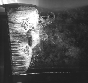
A photo of the CF hydrofoil along with the major dimensions is shown in figure 1. Owing to manufacturing challenges associated with the construction of the small-scale CF hydrofoil, the carbon fibre layers had to be dropped off by approximately 2.5 % of the local chord forward of the trailing edge (TE) at the root, and increased to 11 % of the local chord at the tip, because of thickness limitations. Hence, the glassy-white portion near the TE indicative of the absence of the black carbon fibre layers was larger towards the tip than the root, as observed in figure 1.
(a) CF hydrofoil, labelled with the span and the chord lengths. The coordinate system used for the ROM is also shown, with the origin at the intersection of the EA and the root of the hydrofoil. The black carbon fibre layer is dropped off prior to the foil trailing edge, and the drop off location is increasingly forward of the trailing edge in the outboard portion because of thickness limitations. (b) Diagram of the sectional view of the hydrofoil, along with the definition of the key geometric variables as well as the arrows indicating the positive directions. The variable  $b=c/2$ denotes the semi-chord.

Static testing was performed on the CF hydrofoil to determine the spanwise variation of the elastic axis (EA) relative to the midchord (MC),  $ac$, as defined in figure 1. The test procedure involved placing a weight of 4.3861 kg at different points along the chord and span of the CF hydrofoil and measuring the deflections with a high-resolution camera. At each spanwise coordinate, the EA was determine as the location along the chord where the measured twist was zero. The measured variation of $a$ as a function of the normalized span $\bar {y}=y/s$ is shown in figure 2, where $\bar {y} = 0$ is the root of the hydrofoil and $\bar {y} = 1$ is the tip. The results showed that the EA of the CF hydrofoil shifted from $0.18c$ aft of the midchord at the root to $0.12c$ forward of the midchord at the tip. The spanwise-averaged value of the EA was $\bar {a} =\int _0^{1} a(\bar {y})=-0.0464$, and is used later in the two-degrees-of-freedom (2-DOF) ROM prediction of the steady-state FSI response. Using the same static load measurement procedure, the bending and twisting mode shapes, $f(\bar {y})$ and $g(\bar {y})$, respectively, of the CF hydrofoil were obtained over a trapezoidal grid with 11 chordwise $\times$ 4 spanwise measurement points. As shown in figure 3, the measured mode shapes were independent of chord position, which suggested negligible chordwise deformations. The EA and mode shapes were not measured for the SS hydrofoil because of its high twisting stiffness. Nevertheless, the same fitted functions of the mode shapes, $f(\bar {y})$ and $g(\bar {y})$, as shown in the line legends in figure 3, were used for the SS hydrofoil, as it shares the same undeformed geometry and boundary condition as the CF hydrofoil, and both hydrofoils behaved as linear elastic, isotropic or quasi-isotropic bodies. Here, $a(\bar {y})=0$ was assumed for the SS hydrofoil for simplicity, as it exhibited negligible twist owing to the high twisting stiffness.
Measured variation of the position of the EA from the midchord normalized by the mean chord ( $c = 90$ mm), $a$, of the CF hydrofoil along the normalized spanwise coordinate $\bar {y}$. Forward of the midchord is denoted as negative. The magenta circles denote measurements made along the span. The blue solid line indicates the curve fit (with the equation given in the line legend) of the elastic axis position, while the blue dash–dotted line indicates the spanwise averaged value. It can be seen that the elastic axis is aft of the midchord at the root and moves forward of the midchord at the tip because the carbon fibre layer had to be dropped off forward of the trailing edge owing to thickness limitations. The spanwise-averaged EA value, $\bar {a}$, was used in the ROM predictions.

(a) The bending mode shape,  $f(\bar {y})$, of the CF hydrofoil and (b) the twisting mode shape, $g(\bar {y})$, of the CF hydrofoil. The magenta circles denote the measurements made along the span and the blue lines indicate the fitted mode shapes (with the equation given in the line legend). At each spanwise location, multiple measurements are made along the chord and the data points nearly overlap, which suggests independence from the chordwise coordinate.

Both hydrofoils were manufactured to a  $\pm$0.01 mm surface tolerance and a $0.8\,\mathrm {\mu }\textrm {m}$ surface finish. The composite hydrofoil showed evidence of very minor imperfections on its surface owing to challenges in the moulding process of a relatively thin structure. The minor surface imperfections lead to slightly earlier local cavitation inception in the form of a small bubble streak near the imperfection spot, but it did not affect the developed cavitation response such as in the cloud and supercavitation regimes that are the focus of this work. The effective structural properties of the stiff and flexible hydrofoil can be found in table 1.
Summary of the material and structural properties of the SS and CF hydrofoils (Zarruk et al. Reference Zarruk, Brandner, Pearce and Phillips2014).

2.2. Measurement and data processing techniques
Three different run types, labelled Long, Medium and Short, were conducted for measurement collections. The details of the three run types are summarized in table 2, and detailed information regarding the run types can be found in Part I (Smith et al. Reference Smith, Venning, Pearce, Young and Brandner2020a). Forces were measured in all three run types, while videos for tip deflection and cavitation behaviour were taken in the Medium and Short run types.
Test matrix of the hydrofoils for the various run types detailing the  $\sigma$ range, run duration, $T$, high-speed photography frame rate, $\,f_{{HSP}}$, and force balance sampling rate, $\,f_{{FBS}}$. Long run types provide accurate high frequency resolution loading behaviour with $\sigma$, whereas both statistical and high temporal resolution data of the cavitation behaviour and tip deflection are obtained efficiently with the medium and short run types, respectively. $^{*}$Only conducted for flexible CF hydrofoil.

Tip deflection was measured using a Phantom v2640 high-speed camera with a Nikkor 105 mm f/2.8G lens, operating with a  $512 \times 1504$ pixel resolution for the stiff SS hydrofoil and a $896\times 1504$ pixel resolution for the flexible CF hydrofoil. The spatial resolution of both cases was 0.049 mm px $^{-1}$. Tip deflection was calculated by detecting the edge of the hydrofoil based on peaks in the pixel intensity gradient along each row and comparing the detected edge with that of the hydrofoil under zero load, assuming that the local cross-section of the hydrofoil did not deform. When cavitating tip vortices were observed, the length of the edge was adjusted to exclude the sections of the chord obstructed by the tip vortices to maintain accuracy of the tip deformation measurements. Further details of the edge detection process can be found in Part I (Smith et al. Reference Smith, Venning, Pearce, Young and Brandner2020a). The tip twist, $\theta$, was determined by fitting a line through the detected edge of the hydrofoil tip and subtracting the line from a similar line fitted under the unloaded condition. Tip bending displacement, $\delta$, was obtained as the average distance of each point after twist was subtracted. Positive $\delta$ was defined as bending towards the suction side, and positive $\theta$ was defined as nose-up twist about the midchord.
Cavitation behaviour was recorded using a side-mounted Phantom v2640 high-speed camera with a resolution of  $2048\times 1952$ pixels and a spatial resolution of 0.185 mm px $^{-1}$. Spectral proper orthogonal decomposition (SPOD) was used to identify coherent structures in dynamic cloud cavitation behaviour, using the technique outlined by Towne, Schmidt & Colonius (Reference Towne, Schmidt and Colonius2018). The SPOD method and results have been presented in Parts I (Smith et al. Reference Smith, Venning, Pearce, Young and Brandner2020a) and II (Smith et al. Reference Smith, Venning, Pearce, Young and Brandner2020b) and were obtained by processing a total of 18 000 snapshots for each run.
3. Reduced-order models
To complement the experimental studies, simple ROMs are presented in this section to predict the steady and dynamic FSI response of the hydrofoils. The novelty in the present ROM includes consideration of (1) parametrically oscillating added mass arising from periodic cavity growth and collapse cycles and (2) presence of both re-entrant jet and shock-wave driven cavity shedding frequencies, and random variations in the phase of the unsteady cavity excitation forces arising from the simultaneous presence of two different shedding mechanisms.
The SS and CF hydrofoils are assumed to behave linear elastically and undergo negligible chordwise deformation. Both assumptions are supported by experimental observations reported by Young et al. (Reference Young, Garg, Brandner, Pearce, Butler, Clarke and Phillips2018) and Smith et al. (Reference Smith, Venning, Pearce, Young and Brandner2020a,Reference Smith, Venning, Pearce, Young and Brandnerb). Material bend–twist coupling effects are ignored as the SS hydrofoil is isotropic, and a quasi-isotropic response is expected for the CF hydrofoil. The objective of this section is to present the simplest ROMs that capture the dominant FSI response. Errors arising from the simplified assumptions will be discussed in § 4.
The ROM was derived by decomposing the generalized spanwise bending and twisting deformations,  $\tilde {\delta }(\bar {y},t)$ and $\tilde {\theta }(\bar {y},t)$ as a function of the mode shapes ( $f(\bar {y}$) and $g(\bar {y})$ given in the line legend in figure 3) and time ( $t$):
$t$):
 \begin{equation} \left. \begin{gathered} \tilde{\delta}(\bar{y},t)=\delta(t)f(\bar{y}),\\ \tilde{\theta}(\bar{y},t)=\theta(t)g(\bar{y}), \end{gathered} \right\} \end{equation}
where  $\delta (t)$ and $\theta (t)$ are the tip bending and twisting deformations, respectively, defined at the elastic axis, EA, as shown in figure 1. Using the decomposition shown in (3.1), the generalized equation of motion for $\delta$ and $\theta$ can be derived based on the principle of virtual work, and can be found in Bisplinghoff, Ashley & Halfman (Reference Bisplinghoff, Ashley and Halfman1955) and Akcabay et al. (Reference Akcabay, Chae, Young, Ducoin and Astolfi2014a).
A 2-DOF model was developed to model the steady-state spanwise bending and twisting FSI response, while a 1-DOF model considering only the spanwise bending fluctuations was developed to model the dynamic FSI response. The 1-DOF model was used for the dynamic response because the bending and twisting frequencies were well separated and the twist measurements were contaminated by force balance excitations.
It should be noted that the force balance measurements were about the midchord. The normal force ( $F_N$) was independent of the chordwise position. Equation (3.2) was used to relate the pitch moment at the EA, $F_P^{EA}$, to the value at the midchord, $F_P$:
 \begin{equation} F_P=F_P^{EA}-F_N {\bar{a}c}. \end{equation}
The tip bending and twisting displacements were made about the midchord, but the values were practically the same as at the EA because  $\sin (\theta )\approx 0$ for both hydrofoils. Hence, no effort was made to distinguish the tip deformations about the midchord versus the EA.
3.1. 2-DOF steady-state FSI model
The generalized steady-state 2-DOF model for the spanwise bending and twisting deformations can be written as follows:
 \begin{equation} \begin{bmatrix} \tilde{K}_s^{\delta \delta} & 0 \\ 0 & \tilde{K}_s^{\theta \theta} \end{bmatrix} \begin{bmatrix} \delta \\ \theta \end{bmatrix} = \begin{bmatrix} \tilde{F}_N \\ \tilde{F}_P^{EA} \end{bmatrix}, \end{equation}
where  $\widetilde {K_s}^{\delta \delta }=({EI }/{L^{3}}) \int _0^{1} [ f^{\prime \prime }(\bar {y}) ]^{2}\, \textrm {d}\bar {y}=({EI }/{L^{3}}) \tilde {\beta }_{k \delta }$ and $\widetilde {K_s}^{\theta \theta }=({GJ }/{L}) \int _0^{1} [ g^{\prime }(\bar {y}) ]^{2}\,\textrm {d}\bar {y}=({GJ }/{L}) \tilde {\beta }_{k \theta }$ are the generalized bending and twisting stiffness.
Here,  $E$,
$E$,  $I$,
$I$,  $G$ and $J$ are the material Young's modulus, bending moment of inertia, shear modulus and torsional moment of inertia, as given in table 1. The hydrofoil structural span is $L=316$ mm, which is slightly higher than the hydrodynamic span of $s=300$ mm because of a nominal radial clearance of 0.5 mm between the fairing disk and the test section ceiling penetration to avoid interference with the force measurements (Young et al. Reference Young, Garg, Brandner, Pearce, Butler, Clarke and Phillips2018). Additionally, $\tilde {F}_N=F_N\tilde {\beta }_{fN}$ and $\tilde {F}_P^{EA}=F_P^{EA}\tilde {\beta }_{fP}$ are the generalized normal force (positive upwards) and pitching moment (positive nose-up) defined about the EA.
Defining the combined bending and twisting shape factor as  $\beta _{k \delta }=\tilde {\beta }_{k \delta } /\tilde {\beta }_{fN}$ and $\beta _{k\theta }=\tilde {\beta }_{k \theta }/\tilde {\beta }_{fP}$, (3.3) can be rewritten as follows:
 \begin{equation} \begin{bmatrix} K_s^{\delta \delta} & 0 \\ 0 & K_s^{\theta \theta} \end{bmatrix} \begin{bmatrix} \delta \\ \theta \end{bmatrix} = \begin{bmatrix} F_N=C_N qsc \\ F_P^{EA}=C_P^{EA} qsc^{2} \end{bmatrix}, \end{equation}
where  $K_s^{\delta \delta }=\beta _{k \delta }EI/L^{3}$ and $K_s^{\theta \theta }=\beta _{k\theta }GJ/L$ are the effective structural bending and twisting stiffness, respectively.
Here,  $\beta _{k \delta }$ and $\beta _{k\theta }$ are non-dimensional constants that depend on the geometry only, and account for the spanwise variations of the elastic axis, chord length, load shape distribution and mode shape. Because $EI/L^{3}$ and $GJ/L$ are known for both hydrofoils, $\beta _{k \delta }=5.31$ and $\beta _{k\theta }=0.026$ are determined by taking the slope of the measured normal force ( $F_N$) versus the tip displacement ( $\delta$) and the pitching moment ( $F_P^{EA}$) versus the tip twist angle ( $\theta$) about the elastic axis. The resultant values for $K_s^{\delta \delta }$ and $K_s^{\theta \theta }$ are given in table 3.
Model parameters used in the reduced-order models. The  $K_s^{\delta \delta }$ and $K_s^{\theta \theta }$ are the effective bending and twisting stiffnesses, respectively, $M_s$ is the hydrofoil mass, $\,f_{n1,dry}$ and $\,f_{n1,FW}$ are the dry and fully wetted bending modal frequencies, and $\,f_{n2,dry}$ and $\,f_{n2,FW}$ are the dry and fully wetted twisting modal frequencies.

The mean 3-D normal force and pitching moment coefficients about the EA ( $C_N$ and $C_P^{EA}$) are calculated using (3.5) and (3.6):
 $$\begin{gather} C_N=a_o^{3D} \alpha_{e}=a_o^{3D} \left(\alpha_o+\theta S_g \right), \end{gather}$$
 $$\begin{gather}C_P^{EA}=a_o^{3D} \epsilon \alpha_{e}=a_o^{3D} \epsilon \left(\alpha_o+\theta S_g \right), \end{gather}$$
where  $a_o^{3D} = \partial C_N/\partial \alpha _{e}=a_o^{2D}/( 1+a_o^{2D}/{\rm \pi} A_R )$ is the 3-D lift slope and $a_o^{2D}$ is the two-dimensional (2-D) lift slope, $A_R=2s/c=6.67$ is the effective aspect ratio accounting for the image effect created by the top tunnel boundary at the fixed end of the cantilevered hydrofoil, $\epsilon =e+\bar {a}$ is the spanwise-averaged distance from the CP to the EA normalized by the mean chord, $q=0.5\rho _fU_\infty ^{2}$ is the dynamic fluid pressure, and $\alpha _e=\alpha _o+\theta S_g$ is the effective angle of attack, with $S_g=\int _0^{1} g(\bar {y}) \,\textrm {d}\bar {y}=1/3$.
A semi-empirical equation (3.7) is used to predict the variation of the 2-D lift slope with the effective cavitation parameter  $\psi _e=\sigma /(2\alpha _e)$, where $\sigma =2(p_\infty -p_v)/\rho _f U_\infty ^{2}$:
 \begin{equation} a_o^{2D}={\rm \pi}\left[ \frac{3}{4}\tanh(1.5\psi_e-3)+\frac{5 }{4}\right]. \end{equation}
Note that  $a_o^{2D} \rightarrow 2{\rm \pi}$ for fully wetted flow as $\psi _e \rightarrow \infty$ and $a_o^{2D} \rightarrow {\rm \pi}/2$ for supercavitating flow as $\psi _e \rightarrow 0$. Equation (3.7) is similar in spirit as equation (10) presented by Akcabay & Young (Reference Akcabay and Young2015), and is a simpler mathematical model that follows the trend of experimental data for the 2-D lift slope.
The variation of the maximum attached cavity length to chord length ratio ( $L_c/c$) can be modelled using (3.8), which is obtained by fitting the measured cavity length versus $\psi _e$ of the SS hydrofoil:
 \begin{equation} L_c/c=2.3\exp({-}0.35\psi_e), \end{equation}
where  $e$ is required for the calculation of $\epsilon$ in (3.6), and is the normalized distance from the midchord to the CP, as defined in figure 1. Experimental measurements suggest that $e$ is a function of $L_c/c$ and can be expressed in terms of $\psi _e$:
 \begin{equation} e=e_{FW}-\frac{1 }{6} \exp\left[{-}0.55(\psi_e-2.6)^{2} \right], \end{equation}
where  $e_{FW}=0.26$ is the normalized CP from the midchord in fully wetted flow. Equation (3.9) is obtained by curve fitting the measured CP location of both the SS and CF hydrofoils, as shown later in figure 12.
Defining the fluid stiffness terms as  $K_f^{\delta \theta }=-a_o^{3D}qscS_g$ and $K_f^{\theta \theta }=-a_o^{3D}\epsilon qsc^{2}S_g$, (3.4) can finally be rewritten as follows with all the terms dependent on the unknown tip deformations ( $\delta$ and $\theta$) on the left-hand side:
 \begin{equation} \left( \begin{bmatrix} K_s^{\delta \delta} & 0 \\ 0 & K_s^{\theta \theta} \end{bmatrix} + \begin{bmatrix} 0 & K_f^{\delta \theta} \\ 0 & K_f^{\theta \theta}\end{bmatrix} \right) \begin{bmatrix} \delta \\ \theta \end{bmatrix} = \begin{bmatrix} F_{N,R}=a_o^{3D} \alpha_o q sc \\ F_{P,R}^{EA}=a_o^{3D}\epsilon \alpha_o q sc^{2} \end{bmatrix} , \end{equation}
where  $F_{N,R}$ and $F_{P,R}^{EA}$ are the mean hydrodynamic normal force and pitching moment about the EA for an equivalent rigid hydrofoil at a geometric angle of incidence of $\alpha _{o}$.
3.2. 1-DOF dynamic FSI model
As will be shown later in § 4, the mean tip twist deformation,  $\theta$, is negligible for the SS hydrofoil and very limited ( $\theta <1^{\circ }$) for the CF hydrofoil because of the high stiffness of the small-scale models. In addition, as shown in table 3, the fully wetted twisting modal frequency, $\,f_{n2,FW}$, is much higher and well separated from the fully wetted bending modal frequency, $\,f_{n1,FW}$. Moreover, the twisting modal frequency in water is also higher than the fundamental natural frequency of the force balance, $\,f_{FB}=122$ Hz, used to measure the normal force and pitch moments. Hence, a 1-DOF model is used to simulate the bending fluctuations of the hydrofoils only. The twisting vibrations were neglected, as they were contaminated by the force balance natural frequency.
The tip bending fluctuations ( $\delta ^{\prime }$) are defined as the mean tip bending ( $\delta$) subtracted from the instantaneous tip bending displacement ( $\tilde {\delta }$):
 \begin{equation} \delta^{\prime}=\tilde{\delta}-\delta. \end{equation}
Following the same decomposition as explained above, the equation of motion for the bending fluctuations can be written as follows:
 \begin{equation} M_s\ddot{\delta^{\prime}}+C_s\dot{\delta^{\prime}}+K_s{\delta^{\prime}}=F_{N}^{\prime}, \end{equation}
where  $M_s=f_{ms}\rho _s c^{2} s \tau _c$ and $C_s$ are the effective structural mass and damping, respectively, $\rho _s$ is the solid density as given in table 1, $\tau _c=0.09$ is the maximum thickness-to-chord ratio for the modified NACA0009 cross-section, $\,f_{ms}=0.334$ is a constant shape factor that is the same for both the SS and CF hydrofoils, and $K_s=K_s^{\delta \delta }$ is the effective structural bending stiffness. The values of $M_s$ and $K_s$ are given in table 3, and $C_s$ is assumed to be zero for the sake of simplicity, as structural damping is typically negligible compared with fluid damping. Experimental measurements of the structural damping coefficients ( $\zeta _s=C_s/2\sqrt {K_sMs}$) of different composite, aluminium and PVC hydrofoils were found to be between 1 % and 2 % (Phillips et al. Reference Phillips, Cairns, Davis, Norman, Brandner, Pearce and Young2017; Harwood et al. Reference Harwood, Felli, Falchi, Garg, Ceccio and Young2020). However, the fully wetted damping coefficients for the first (bending) mode were more than an order of magnitude higher than the structural damping coefficients according to experimental measurements presented by Blake & Maga (Reference Blake and Maga1975), Phillips et al. (Reference Phillips, Cairns, Davis, Norman, Brandner, Pearce and Young2017) and Harwood et al. (Reference Harwood, Felli, Falchi, Garg, Ceccio and Young2020).
The  $F_N^{\prime }$ in (3.12) is the fluctuating normal hydrodynamic force, which is linearly decomposed into a component associated with unsteady cavity shedding on an equivalent rigid hydrofoil, $F_{R}^{\prime }$, and a component arising from the FSI, $F_{FSI}^{\prime }$:
 $$\begin{gather} F_N^{\prime}=F_{R}^{\prime}+F_{FSI}^{\prime} = C_N^{\prime} qsc, \end{gather}$$
 $$\begin{gather}F_{FSI}^{\prime}={-}( \hat{M}_f\ddot{\delta^{\prime}}+C_f\dot{\delta^{\prime}}+K_f{\delta^{\prime}} ), \end{gather}$$
where  $\hat {M}_f$, $C_f$ and $K_f$ are the fluid inertial, damping and disturbing force terms in phase with the fluctuating bending acceleration, velocity and displacement, respectively, and $C_N^{\prime }$ is the fluctuating normal force coefficient for the flexible hydrofoil.
By moving the FSI forces to the left-hand side, (3.12) can be rewritten as follows:
 \begin{equation} (M_s+\hat{M}_f )\ddot{\delta^{\prime}}+\left(C_s+C_f\right)\dot{\delta^{\prime}}+\left(K_s+K_f \right){\delta^{\prime}}=F_{R}^{\prime}. \end{equation}
 Because only the bending DOF is considered,  $K_f=0$ according to (3.10) and potential flow, i.e. pure bending or heave displacement perpendicular to the flow, does not affect the normal force.
The fluctuating normal force arising from unsteady cavity shedding on a rigid hydrofoil can be modelled as simple sinusoidal oscillations at the cavity shedding frequencies:
 \begin{equation} F_{R}^{\prime}=F_{Ro}^{\prime} \left[ \sin(2{\rm \pi} f_{c1}t+\phi_1)+\sin(2{\rm \pi} f_{c2}t+\phi_2) \right]=C_R^{\prime} qsc, \end{equation}
where  $\,f_{c1}$ and $\,f_{c2}$ are the Type I shock-wave-driven and Type II re-entrant jet-driven cavity shedding frequencies, respectively, $\phi _1$ and $\phi _2$ are random phase variations between $0$ and ${\rm \pi}$, and $C_R^{\prime }$ is the fluctuating normal force coefficient for an equivalent rigid hydrofoil. The cavity oscillation force is typically not exactly a sinusoid, but rather a biased wave form with a longer cavity growing process than the breakdown process. However, a sinusoid is used as it is the simplest and lowest order function that captures the dominant frequency. This is desired as there are two cavity shedding frequencies, one associated with the re-entrant jet and the other with the shock-wave. A more complicated wave form would require more empirical coefficients.
The amplitude of the normal force coefficient,  $C_{Ro}^{\prime }$, is modelled as follows:
 \begin{equation} C_{Ro}^{\prime}=\frac{F_{Ro}^{\prime}}{qsc}= \frac{1 }{15} \exp({-}0.7(\psi_e-2.8)^{2}). \end{equation}
Note that  $C_{Ro}^{\prime } \rightarrow 0$ for $\psi _e \rightarrow \infty$ and $C_{Ro}^{\prime } \sim 0$ for $\psi _e = 0$, i.e. the fluctuations decay to zero in stable fully wetted (and fully attached because $\alpha _o=6^{\circ }$) flow and in stable supercavitating flow (which typically requires $L_c/c>1.5$). Because the fluctuating normal force amplitude depends on the extent of cavitation, $\psi _e$ is used in (3.17) to account for differences in the mean effective incidence, $\alpha _e$, caused by the change in mean tip twist, $\theta$. Equation (3.17) gives the fluctuating normal force coefficient for an equivalent rigid hydrofoil, and is obtained by curve fitting the measured standard deviation of the fluctuating normal force for the SS hydrofoil (as it underwent only minor bending and negligible twisting deformation, as shown in figure 10). The comparison between the values given by (3.17) (blue dashed line) and the measured value ( $C_{N,SD}^{\prime }$ shown by the blue solid line with filled blue circles) is shown later in figure 25(a).
Experimental data presented in Parts I (Smith et al. Reference Smith, Venning, Pearce, Young and Brandner2020a) and II (Smith et al. Reference Smith, Venning, Pearce, Young and Brandner2020b), and in previous literature, indicate that the Type I shock-wave-driven cavity shedding frequency is between 10 and 12 Hz and varies approximately linearly with the cavitation parameter over a limited cavitation parameter range:
 \begin{equation} f_{c1}=10+\frac{(\psi_e-0.9) }{1.2}\,\textrm{Hz}\quad \textrm{for}\ 0.9 \le \psi_e \le 3.3. \end{equation}
Type I shedding tends to have a more uniform cavity shedding pattern and frequency along the span, such as shown later in figure 6(a) for  $\sigma =0.3$ for the SS hydrofoil. As noted in § 1, Types I and II shedding can occur simultaneously in different portions of the span, or interact with each other over time, which leads to arbitrary phase difference and hence the need for $\phi _1$ and $\phi _2$ in (3.16).
Type I cavity shedding only occurs over a limited range of cavitation parameter ( $0.9 \le \psi _e \le 3.3$), as the vapour volume fraction has to be just right (near 0.5–0.6 according to Shamsborhan et al. Reference Shamsborhan, Coutier-Delgosha, Caignaert and Nour2010; Ganesh et al. Reference Ganesh, Mäkiharju and Ceccio2016) to reduce the speed of sound of the fluid mixture such that shocks can form in flows with speeds of the order of $10\,\textrm {m}\,\textrm {s}^{-1}$ or less. For $\psi _e>3.3$, only Type II cavity shedding exists, so (3.16) becomes $F_{R}^{\prime }=F_{Ro}^{\prime } \sin (2{\rm \pi} f_{c2}t+\phi _2)$.
Based on experimental data presented in Parts I (Smith et al. Reference Smith, Venning, Pearce, Young and Brandner2020a) and II (Smith et al. Reference Smith, Venning, Pearce, Young and Brandner2020b), two modes of Type II cavity oscillations were observed. SPOD analysis of the high-speed videos indicated that the primary re-entrant jet-driven shedding mode, called Type IIa, is confined to the inboard portion of the span, while Type IIb is the secondary re-entrant jet shedding mode with shedding near the outboard portion of the span. Examples of Types IIa and IIb re-entrant jet-driven shedding can be observed in figures 6( f) and 7( f) for  $\sigma =0.8$ for the SS and CF hydrofoils, respectively. The cavity length and cavity shedding frequency is non-uniform along the span owing to spanwise load variations caused by 3-D effects. Because the amplitude of the Type IIb shedding was observed to be much weaker than the Type IIa shedding, only Type IIa shedding is considered in the simplified 1-DOF model, and is called Type II shedding from here on.
Experimental results presented in Parts I (Smith et al. Reference Smith, Venning, Pearce, Young and Brandner2020a) and II (Smith et al. Reference Smith, Venning, Pearce, Young and Brandner2020b) suggested the following relationship for the Type II re-entrant jet-driven cavity shedding frequency:
 \begin{equation} St_2=\frac{f_{c2} c }{U_\infty}=0.0045\psi_e^{3}+0.12. \end{equation}
Note that  $\psi _e$ is used in both (3.18) and (3.19) to account for the difference in the effective angle of incidence, $\alpha _e$, caused by the mean tip twist, $\theta$.
The fluid added mass,  $\hat {M}_f$, oscillates with the periodic growth and collapse of the cavity owing to changes in the density of the local fluid mixture. For the sake of simplicity, $\hat {M}_f$ is assumed to be modulated by the Type II re-entrant jet cavity shedding frequency only:
 $$\begin{gather} \hat{M}_f(t)={M_{f}} \left[1+\epsilon_m \sin(2{\rm \pi} f_{c2}t) \right], \end{gather}$$
 $$\begin{gather}M_f=\frac{M_f^{FW} }{1- \epsilon_m} ,\quad \epsilon_m=\frac{1 }{6} \left[ \tanh(\psi_e-3.4)-1 \right], \end{gather}$$
where  $M_f$ is the effective mean fluid added mass for bending deformation, and $M_f^{FW}=f_{mf}{\rm \pi} \rho _fc^{2}s/4$ is the effective fluid added mass in fully wetted flow, with $\,f_{mf}=0.47$ as a constant bending shape factor for both hydrofoils. Note that the upper limit of $\hat {M}_f$ corresponds to the fully wetted value, i.e. $M_{f,max}=M_f^{FW}$, while the lower limit of $\hat {M}_f$ decreases with decreasing effective cavitation parameter $\psi _e$, as more dense liquid is replaced by much lighter vapour on the suction side. Here, $M_{f,min} \rightarrow 0.5M_f^{FW}$ as $\psi _e \rightarrow 0$, as the entire suction side of the hydrofoil would be enveloped inside the vaporous cavity in supercavitating flow. The variation of the fluid-to-solid mass ratio, $\hat {M}_f/M_s$, of the SS and CF hydrofoils are shown in figure 4(a).
Variation of the predicted fluid added mass to (a) solid mass ratio ( $\hat {M}_f/M_s$), (b) system bending frequency ( $\hat {f}_{n1}$) and (c) fluid damping coefficient ( $\zeta _f$) with cavitation number ( $\sigma$) for the SS and CF hydrofoils. The mean fluid added mass decreases with decreasing $\sigma$, as more water on the suction side is replaced by lighter vapour. The fluid added mass fluctuates between the maximum ( $M_{f,max}=M_f^{FW}$) and minimum ( $M_{f,min} \rightarrow 0.5M_{f}^{FW}$ as $\sigma \rightarrow 0$) values with periodic cavity shedding, and is determined using (3.21). Modulation in the fluid added mass leads to modulation in the system bending frequency, $\hat {f}_{n1}$, which fluctuates between $\,f_{n1,min}=f_{n1,FW}$ and $\,f_{n1,max}$, with $\,f_{n1,max} \rightarrow \sqrt {K_s/(M_s + 0.5M_f^{FW})}$ as $\sigma \rightarrow 0$ following (3.22). These values are used when denoting $\,f_{n1}$ limits throughout this work. The mean system bending frequency and the bandwidth of frequency modulation both increase with decreasing cavitation number. The fluid damping coefficient is obtained using (3.23), and $\zeta _f$ is higher for the CF hydrofoil because of the lower mean system bending frequency, $\,f_{n1}$.

Because  $K_f=0$, the eigenvalue solution of (3.15) yields the following for the system bending frequency:
 \begin{equation} \hat{f}_{n1}=\sqrt\frac{K_s }{\left(M_s+\hat{M}_f \right)}. \end{equation}
Because  $\hat {M}_f$ modulates with periodic cavity shedding, $\hat {f}_{n1}$ will modulate as well. The lower limit of the system bending frequency, $\,f_{n1,min}$, corresponds to the fully wetted value, $\,f_{n1,FW}=\sqrt {K_s / (M_s+M_f^{FW} )}$, while the upper limit, $\,f_{n1,max}$, increases with decreasing effective cavitation parameter because of the reduction in fluid added mass, with $\,f_{n1,max} \rightarrow \sqrt {K_s/(M_s + 0.5M_f^{FW})}$ as $\psi _e \rightarrow 0$. Variation of the predicted system bending frequency is shown in figure 4(b). Here, $\,f_{n1}$ denotes the mean system bending frequency based on the mean fluid added mass, $M_f$. Note that $\,f_{n1}$ is not the average of $\,f_{n1,max}$ and $\,f_{n1,min}$ because of the presence of the solid mass $M_s$ in the denominator of (3.22).
As shown in figure 4, the fluid added mass has a much greater impact on the system bending frequency of the CF hydrofoil than the SS hydrofoil because of the higher fluid added mass to solid mass ratio ( $\hat {M}_f/M_s$), which varied between 3.8 and 7.5 for the CF hydrofoil and between 1.1 and 1.6 for the SS hydrofoil. Consequently, while the dry bending frequency ( $\,f_{n1,dry}=\sqrt {K_s / M_s}$) of the CF hydrofoil (121 Hz) is higher than that of the SS hydrofoil (94 Hz), the fully wetted bending frequency ( $\,f_{n1,FW}$) of the CF hydrofoil (41 Hz) is lower than that of the SS hydrofoil (58 Hz). A summary of the modelled system parameters are given in table 3. Another important observation from figure 4 is that the mean system bending frequency and the bandwidth of frequency modulation both increase with decreasing cavitation number.
The fluid damping coefficient,  $\zeta _f$, is assumed to be a linear function of the mean system bending frequency. Following Blake & Maga (Reference Blake and Maga1975) and assuming a nearly 2-D response, the fluid damping coefficient is obtained using (3.23):
 \begin{equation} \zeta_f=\frac{C_s+C_f }{2 \sqrt{(M_s+M_f) K_s}}=\frac{U_\infty }{2 f_{n1} c}. \end{equation}
Because structural damping is ignored (i.e.  $C_s=0$) in the current model, the fluid damping coefficient, $\zeta _f$, is also the total damping coefficient. Note that the mean fluid added mass, $M_f$, and the mean system bending frequency, $\,f_{n1}$, are used when computing the damping coefficient with (3.23) for simplicity. Variation of $\zeta _f$ for the SS and CF hydrofoils are shown in figure 4(c). As shown in the figure, the fluid damping coefficient is much greater than a typical structural damping coefficient of 0.01–0.02.
Note that with periodic oscillations in  $\hat {M}_f$, (3.15) represents a 1-DOF forced parametric oscillator and is responsible for the nonlinear response of the system. Parametric resonance can develop if the modulation (Type II cavity shedding) frequency is two times the system natural frequency, i.e. $\,f_{c2}=2f_{n1}$, and is discussed by Akcabay & Young (Reference Akcabay and Young2015). However, for the small model-scale SS and CF hydrofoils, parametric resonance will not occur because of the high value of $\,f_{n1}$ associated with high hydrofoil stiffness, low amplitude of modulation and high fluid damping.
4. Results
4.1. Modal frequencies
To verify the system parameters used in the ROMs presented in § 3, the predicted system modal frequencies are compared with experimental measurements of the SS and CF hydrofoils in fully wetted conditions in figure 5. The experimental measurements of  $C_N^{\prime }$ were averaged for incidences ( $\alpha _o$) ranging from $0^{\circ }$ to $14^{\circ }$ in increments of $2^{\circ }$ in non-cavitating (fully wetted or FW) conditions at $Re=0.6\times 10^{6}$. The average power spectral density (PSD) was used, as the frequency at the peak of the PSD varied slightly with $\alpha _o$ owing to changes in entrained fluid inertia, particularly when stall develops for $\alpha _o \gtrsim 10^{\circ }$ (Zarruk et al. Reference Zarruk, Brandner, Pearce and Phillips2014; Young et al. Reference Young, Garg, Brandner, Pearce, Butler, Clarke and Phillips2018). No frequency modulations were observed in fully wetted conditions. It should be noted that in the experimental studies presented by Zarruk et al. (Reference Zarruk, Brandner, Pearce and Phillips2014), the same hydrofoils with the same mounting set-up and force balance (FB) were used in the same cavitation tunnel. The FB frequency was 122 Hz, which is significantly higher than the first FW bending frequency, $\,f_{1,FW}$, of 58 Hz for the SS hydrofoil and 41 Hz for the CF hydrofoil. As noted in § 3, the dynamic FSI response was modelled using a 1-DOF forced parametric oscillator model considering spanwise bending only. The dynamic model can be extended to 2-DOF, which would yield dry ( $\,f_{n2,dry}$) and fully wetted ( $\,f_{n2,FW}$) second mode (twisting) frequencies as presented in table 3. The $\,f_{n2,FW}$ is also shown in figure 5.
Measured (Exp) averaged power spectral density (PSD) of the fluctuating normal force coefficients ( $C_N^{\prime }$) for the SS and CF hydrofoils for incidences ( $\alpha _o$) ranging from $0^{\circ }$ to $14^{\circ }$ in increments of $2^{\circ }$ in non-cavitating conditions at $Re=0.6\times 10^{6}$ (Zarruk et al. Reference Zarruk, Brandner, Pearce and Phillips2014). The vertical lines correspond to the predicted first and second system bending natural frequencies in fully wetted condition, $\,f_{1,FW}$ and $\,f_{2,FW}$, for the SS and CF hydrofoils, their visible harmonics and the measured averaged force balance (FB) natural frequency, $\,f_{FB}$. Good agreement is observed between the predicted modal frequencies and the location of the peaks of the frequency spectra, especially considering that the measured PSD varies slightly with $\alpha _o$ owing to changes in entrained fluid inertia, particularly when stall develops with $\alpha \gtrsim 10^{\circ }$ (Zarruk et al. Reference Zarruk, Brandner, Pearce and Phillips2014; Young et al. Reference Young, Garg, Brandner, Pearce, Butler, Clarke and Phillips2018).

As shown in figure 5, good agreement was observed between the predicted modal frequencies and the location of the peaks of the averaged PSD of the  $C_N^{\prime }$ reported by Zarruk et al. (Reference Zarruk, Brandner, Pearce and Phillips2014). Figure 5 demonstrates that the FW twisting frequency was much higher than the FW bending frequency, and hence the separation of time scale justifies the use of the 1-DOF dynamic model considering the bending degree of freedom only.
4.2. Cavitation patterns
Examples of the observed cavitation patterns of the SS and CF hydrofoils at selected cavitation numbers are shown in figures 6 and 7, respectively. The corresponding variation of the measured maximum local attached cavity length normalized by the local chord at each section ( $L_{c}(y)/c(y$)) with $\sigma$ for the SS and CF hydrofoils are shown in open circles and cyan filled squares, respectively, in figure 8. The predicted cavity length normalized by the mean chord ( $L_{c}/c$) obtained using (3.8) for the SS and CF hydrofoils are shown as a blue dashed line and a magenta dash–dotted line, respectively.
Typical example images of cavitation of the SS hydrofoil at selected values of  $\sigma$. (a) Type I shock-wave-driven cavity shedding only at $\sigma = 0.3$.(b–d) Combined Type II re-entrant jet and Type I shock-wave-driven cavity shedding for $0.4 \lesssim \sigma \lesssim 0.6$. (e–h) Type II re-entrant jet cavity shedding only for $0.7 \lesssim \sigma \lesssim 1.0$. Tip vortex cavities can be observed for $0.3 \lesssim \sigma \lesssim 0.7$ in panels (a–e): (a) $\sigma =0.3$; (b) $\sigma =0.4$; (c) $\sigma =0.5$; (d) $\sigma =0.6$; (e) $\sigma =0.7$; ( f) $\sigma =0.8$; (g) $\sigma =0.9$; (h) $\sigma =1.0$.

Typical example images of cavitation of the CF hydrofoil at selected values of  $\sigma$. (a) Type I shock-wave-driven cavity shedding only at $\sigma = 0.3$. (b–d) Combined Type II re-entrant jet and Type I shock-wave-driven cavity shedding for $0.4 \lesssim \sigma \lesssim 0.6$. (e–h) Type II re-entrant jet cavity shedding only for $0.7 \lesssim \sigma \lesssim 1.0$. Compared with the cavitation patterns for the SS hydrofoil shown in figure 6, the maximum attached cavity length is slightly longer for the CF hydrofoil for $\sigma \gtrsim 0.7$. Moreover, the cavities extend all the way to the tip for $\sigma \lesssim 1.0$ for the CF hydrofoil, but only for $\sigma \lesssim 0.7$ for the SS hydrofoil. Tip vortex cavities can also be observed for $0.3 \lesssim \sigma \lesssim 0.7$ in panels (a–e): (a) $\sigma =0.3$; (b) $\sigma =0.4$; (c) $\sigma =0.5$; (d) $\sigma =0.60$; (e) $\sigma =0.7$; ( f) $\sigma =0.8$; (g) $\sigma =0.9$; (h) $\sigma =1.0$.

Variation of the measured (Exp, based on data presented by Smith et al. Reference Smith, Venning, Pearce, Young and Brandner2020b) and the modelled (Pre, obtained using (3.8)) normalized attached cavity length ( $L_c/c$) with the cavitation number ( $\sigma$). The measured values correspond to the maximum local attached cavity length normalized by the local chord at different normalized spanwise locations ( $y/s$) and are shown in open circles and cyan filled squares for the SS and CF hydrofoils, respectively. The modelled values for the SS and CF hydrofoils, obtained using (3.8), are shown as a blue dashed line and a magenta dash–dotted line, respectively. The cavity length is slightly longer for the CF hydrofoil than the SS hydrofoil for $\sigma \gtrsim 0.7$ because the CF hydrofoil has a higher effective angle of incidence owing to flow-induced nose-up twist.

In general, cloud cavitation was observed on both hydrofoils for  $0.3 \lesssim \sigma \lesssim 1.0$, and supercavitation for $\sigma \lesssim 0.3$. For $1.0 \lesssim \sigma \lesssim 1.2$, relatively stable partial leading edge sheet cavitation was observed for the SS hydrofoil, while unsteady cloud cavitation was observed for the CF hydrofoil. The earlier transition of the CF hydrofoil to cloud cavitation was primarily owing to the higher effective angle of incidence caused by the nose-up twist allowed by the greater twisting flexibility of the CF hydrofoil. It is important to note that while the imperfect surface finish of the CF hydrofoil triggered local bubble cavitation inception, it did not impact the global cavitation behaviour, particularly in the cloud and supercavitation regimes.
Figures 6(e–h) and 7(e–h) show Type II re-entrant jet cavity shedding on the SS and CF hydrofoils, respectively, for  $0.7 \lesssim \sigma \lesssim 1.0$. Figures 6(b–d) and 7(b–d) show combined Type II re-entrant jet and Type I shock-wave-driven cavity shedding on the SS and CF hydrofoils, respectively, for $0.4 \lesssim \sigma \lesssim 0.6$. Figures 6(a) and 7(a) show Type I shock-wave-driven cavity shedding only at $\sigma = 0.3$. Relatively stable supercavitation was observed when $\sigma <0.3$ ( $L_c/c\gtrsim 1.5$), but it is not shown in figures 6 and 7 to be succinct. Interested readers should refer to Parts I (Smith et al. Reference Smith, Venning, Pearce, Young and Brandner2020a) and II (Smith et al. Reference Smith, Venning, Pearce, Young and Brandner2020b) for more detailed images, including a breakdown of the Type I and Type II cavity shedding mechanics, frequencies and phase plots.
Figure 8 shows good general agreement between the predicted and measured maximum attached cavity length, which increases with decreasing  $\sigma$. An inflection point is observed in the measured maximum attached cavity length ( $L_c/c$) when $\sigma \approx 0.7$ or $L_c/c \approx 0.8$. Here, $\sigma \approx 0.7$ corresponds to when shock-wave-driven cavity shedding was first observed as the cavitation number was lowered for both hydrofoils. There was a reduction in the cavity length growth rate for $0.4 \lesssim \sigma \lesssim 0.6$, which corresponds to $L_{c}/c = 1.0$, at which the cavity closure interacts with flow from the pressure side of the hydrofoil (Smith et al. Reference Smith, Venning, Pearce, Young and Brandner2020a,Reference Smith, Venning, Pearce, Young and Brandnerb).
As shown in figures 6–8, the CF hydrofoil exhibited slightly longer cavities than the SS hydrofoil because of a higher nose-up twist for  $L_c/c \lesssim 0.8$ or $\sigma \gtrsim 0.7$. The small difference between the SS and CF hydrofoil arose from the offset of the higher twisting flexibility of the CF hydrofoil by the reduced moment arm, as the mean EA of the CF hydrofoil was upstream of the midchord (i.e. $\bar {a}<0$, as shown in figure 2). The $L_c/c$ was nearly the same for both hydrofoils when $\sigma \lesssim 0.7$ because of the limited pitching moment in supercavitating flow. It can also be seen in figure 8 that $L_c/c$ differed the most between the SS and CF hydrofoils for the measurement points farthest away from the root, e.g. $y/s = 0.6~and~0.8$, where spanwise bending and twist deflection were the highest. Comparison of the cavitation patterns in figures 6(e–h) and 7(e–h) indicated that while the cavity extended across the entire span of the CF hydrofoil, including at the tip, for $\sigma \lesssim 1.0$, the cavity did not extend all the way to the tip of the SS hydrofoil until $\sigma \lesssim 0.7$. Another noteworthy observation from figures 6 and 7 is the presence of the tip vortex cavities for $0.3 \lesssim \sigma \lesssim 0.7$ for both hydrofoils.
4.3. Mean performance and histograms in cloud cavitation
The measured variation of the mean normal force ( $C_N$) and mean pitch moment ( $C_P$) coefficients about the midchord, and normalized CP from midchord ( $e$) with cavitation number ( $\sigma$) are shown as black open circles for the SS and CF hydrofoils in figure 9. The magenta lines in figure 9 correspond to the measured histograms in the form of probability density functions at each $\sigma$. In general, the mean $C_N$ and $C_P$ reduce as the cavity lengthens. The local maximum in $C_N$ occurs at $\sigma \approx 0.7$ or $L_c/c \approx 0.8$ because of the large partial cavity maximizing the virtual camber effect while being just far enough away from the hydrofoil trailing edge such that it does not significantly modify the flow (and hence pressure) on the pressure side of the hydrofoil. Note that $\sigma \approx 0.7$ or $L_c/c \approx 0.8$ is also where an inflection point can be observed on $L_c/c$ in figure 8. As $\sigma$ decreases from 0.7, the cavity lengthens to reach the hydrofoil trailing edge and beyond, which causes the pressure on the pressure side to lower and reach the vapour pressure at the hydrofoil trailing edge (as required by the Kutta condition when it is covered by the vaporous cavity). The lower net pressure difference leads to a reduction in $C_N$. However, as $\sigma$ increases from 0.7, $L_c/c$ decreases, which reduces the virtual camber effect, as well as the effect of the cavity on the suction side pressure distribution. Hence, $C_N$ gradually reduces and approaches the fully wetted value as $\sigma$ further increases from 0.7. Note that the reduction in $C_P$ occurs earlier (at a higher $\sigma$) because of the shift in CP towards the midchord ( $e \rightarrow 0$) as $L_c/c \rightarrow 1$. The mean $e$ reaches a minimum near $\sigma \approx 0.6$, which corresponds to when $L_c/c \approx 1.0$ according to figure 8. For $\sigma <0.6$, the mean CP shifts back towards the quarter chord position because of increases in the suction side pressure caused by the re-entrant jet and shock-wave induced shedding. The shedding and breakdown of the low-pressure vaporous cavity shift upstream because shock-waves travel faster and further upstream than the re-entrant jet. This explains the trend for the mean value of $e$ and the sustained high amplitude of fluctuations in $e$ for $\sigma <0.6$.
Variation of the measured mean normal force ( $C_N$) and mean pitch moment ( $C_P$) coefficients about the midchord, and normalized centre of pressure (CP) from midchord ( $e$) with cavitation number ( $\sigma$) are shown as black open circles for the SS (a,c,e) and CF (b,d, f) hydrofoils. The magenta lines correspond to the measured histograms in the form of probability density functions at each $\sigma$. In general, the mean $C_N$ and $C_P$ reduces as $\sigma$ reduces, but the drop in $C_P$ occurs at a higher $\sigma$ than $C_N$ because of the reduction in $e$. The load fluctuations initially increase as the cavity lengthens with reduction in $\sigma$, and reach a maximum when the cavity approaches the hydrofoil trailing edge ( $\sigma \approx 0.6$), which corresponds to when $e$ is the lowest (the CP is nearest to the midchord). For $\sigma <0.6$, the load fluctuations decrease as supercavitation develops with further reduction in $\sigma$, while $e$ increases to near the fully wetted value, as the re-entrant jet- and shock-wave-driven cavity shedding lead to a higher suction side pressure upstream of the trailing edge.

There is minimal load fluctuations for when  $\sigma \gtrsim 1.0$ for the SS hydrofoil and $\sigma \gtrsim 1.1$ for the CF hydrofoil. Fluctuations begin at a higher $\sigma$ for the CF hydrofoil because of an earlier transition to cloud cavitation, consistent with experimental observations reported in Part II (Smith et al. Reference Smith, Venning, Pearce, Young and Brandner2020b) and with the slightly longer cavity observed in figure 8. The load fluctuations initially increase as the cavity lengthens with a reduction in $\sigma$, and reach a maximum when the cavity approaches the hydrofoil trailing edge ( $\sigma \approx 0.6$). For $\sigma <0.6$, the load fluctuations decrease as supercavitation develops with a further reduction in $\sigma$. The variation of the amplitude of the fluctuating normal force coefficients is captured by (3.17), where the fluctuations decay to zero ( $C_{Ro}^{\prime } \rightarrow 0$) in stable supercavitation as $\psi _e \rightarrow 0$ and in fully wetted flow as $\psi _e \rightarrow \infty$. The highest fluctuation in $C_N$ and $C_P$ is observed at $\sigma \approx 0.6$ or $L_c/c \approx 1$, which corresponds to $\psi _e \approx 2.8$ with $\alpha _e = 6^{\circ }$, consistent with the local maxima that can be obtained by taking the derivative of (3.17) with $\psi _e$.
The measured variation of the mean normalized tip bending deflection ( $\delta /c$) and tip twist angle ( $\theta$) with $\sigma$ are shown as black open circles for the SS and CF hydrofoils in figure 10. The magenta lines correspond to the measured histograms in the form of probability density functions at each $\sigma$. Comparison with figure 9 shows that, in general, the trend for $\delta$ follows $C_N$, and the trend for $\theta$ follows $C_P$, as the hydrofoils behave linear elastically. Both hydrofoils underwent slight bending towards the suction side. Compared with the CF hydrofoil, the SS hydrofoil experiences a much lower mean amplitude of tip bending and twisting deformations, which is expected because of the higher bending and twisting stiffness values ( $K_s^{\delta \delta }$ and $K_s^{\theta \theta }$). In particular, the tip twist of the SS hydrofoil is near $0^{\circ }$, i.e. negligible. In fully wetted and partially cavitating flows, the CF hydrofoil undergoes nose-up twist, $\theta >0$ for $\sigma >0.75$ in figure 10. Here, $\theta$ reduces as $\sigma$ reduces to near 0.6 because of the reduction in $e$ (i.e. CP moving towards the midchord), and reaches a minimum at $\sigma \approx 0.6$ with $e \approx 0.1$. Additionally, $\theta <0$ for $0.4 \lesssim \sigma \lesssim 0.7$ because the CP is shifted to aft of the EA at the tip ( $e < 0.12$), causing a nose-down twist. This is because the EA at the tip is noticeably forward of the midchord ( $a(\bar {y}=1)=-0.12$, as shown in figure 2). Last, $\theta \approx 0$ for $\sigma \le 0.3$ because of the low value of $C_P$ in supercavitating flow.
Variation of the measured the mean normalized tip bending deflection ( $\delta /c$) and tip twist angle ( $\theta$) with cavitation number ( $\sigma$) are shown as black open circles for the SS (a,c) and CF (b,d) hydrofoils. The magenta lines correspond to the measured histograms in the form of probability density functions at each $\sigma$. In general, the trend for $\delta$ follows $C_N$, and the trend for $\theta$ follows $C_P$, as the hydrofoils behave linear elastically. The SS hydrofoil experiences a much lower mean amplitude of tip deformations because of the higher stiffness compared with the CF hydrofoil. In fully wetted flow, the CF hydrofoil undergoes nose-up twist, but $\theta$ reduces as $\sigma$ reduces to near 0.6 because of the reduction in $e$ (i.e. CP moving towards the midchord). Here, $\theta <0$ for $0.3 \lesssim \sigma \lesssim 0.75$ because the CP is shifted to aft of the EA at the tip, which causes a slight nose-down twist. Additionally, $\theta \approx 0$ for $\sigma \le 0.3$ because of the low value of $C_P$ in supercavitating flow.

The measured histograms of  $C_P$ and $e$ in figure 9, as well as $\theta$ in figure 10, exhibit increasing peakiness, or Kurtosis, as $\sigma$ decreases from 0.7, which is the cavitation number when shock-wave-driven cavity shedding was first observed. The results are consistent with the physical observations that shock-wave-driven cavity shedding is more coherent along the span, while re-entrant jet cloud cavity shedding exhibits more 3-D variations along the span. In addition, Type II subharmonic lock-in occurs on both hydrofoils at $\sigma \approx 0.7$, which may contribute to the large fluctuations in normal force.
The histograms of the normal force coefficient ( $C_N$) and tip bending displacement ( $\delta$) show similar behaviour to $C_P$ and $\theta$, respectively, except at $\sigma =0.4$ for the CF hydrofoil, where a bi-modal response is observed in figures 9 and 10. The bi-modal response is caused by the strong presence of Type I and Type II cavity shedding, and by lock-in of the Type I cavity shedding frequency with the nearest subharmonic of the system bending frequency of the CF hydrofoil. The subharmonic lock-in will be explained in more detail in § 4.5.
4.4. Steady-state FSI response in cavitating flow
Comparisons of the measured and predicted mean normal force ( $C_N$) and mean pitch moment ( $C_P$) coefficients about the midchord, as well as normalized tip bending deflection ( $\delta /c$) and mean tip twist angle ( $\theta$), for the SS and CF hydrofoils are shown in figure 11. The measured and predicted normalized position of the CP from the midchord, $e$, are shown in figure 12. The experimental data for the SS and CF hydrofoils are shown by blue open circles and magenta open squares, respectively. The predictions obtained using the 2-DOF steady-state FSI model presented in § 3.1 are shown as blue dashed lines and magenta dash–dotted lines for the SS and CF hydrofoils, respectively.
(a,c) Comparison of the measured and predicted mean normal force ( $C_N$) and mean pitch moment ( $C_P$) coefficients about the michord, and (b,d) normalized tip bending deflection ( $\delta /c$) and mean tip twist angle ( $\theta$), with cavitation number ( $\sigma$). The experimental data for the SS and CF hydrofoils are shown by blue open circles and magenta open squares, respectively. Good agreement is observed between the predictions and measurements for $C_N$, $C_P$ and $\delta /c$ for both hydrofoils. There is good agreement on the trend of the $\theta$ between prediction and measurement, but the amplitude is under-predicted because the spanwise-averaged normalized elastic axis position from the midchord, $\bar {a}$, is used in the prediction.

Variation of the measured and fitted normalized distance of the CP from the midchord,  $e$, with cavitation number ( $\sigma$). The experimental data for the SS and CF hydrofoils are shown by blue open circles and magenta open squares, respectively. The values predicted by (3.9) for the SS and CF hydrofoils are shown as blue dashed lines and magenta dash–dotted lines, respectively. As $\sigma$ reduces toward 0.6, $e$ lowers as the CP moves toward the midchord as $L_c/c \rightarrow 1$. As $\sigma$ further reduces from 0.6 and $L_c/c>1$, the CP moves back toward the quarter chord.

In general, good agreement is observed between the predictions and measurements of the mean hydrodynamic loads and deformations. The SS hydrofoil underwent some bending deformation with negligible twist, with the maximum mean tip bending deflection ( $\delta$) less than 5 % of the mean chord length ( $c$). The CF hydrofoil underwent greater bending deflection, with the maximum value being approximately 11.4 % of the mean chord. The SS hydrofoil exhibited negligible twist. In fully wetted and partially cavitating flow, the CF hydrofoil exhibited nose-up twist at the tip, as the CP was upstream of the EA. The nose-up twist was responsible for the slightly higher values of $L_c/c$, $C_N$ and $C_P$ of the CF hydrofoil. The higher nose-up twist, which was maximum at the free tip, was also why the cavity extended across the entire span of the CF hydrofoil for $\sigma \lesssim 1.0$, but only for $\sigma \lesssim 0.7$ for the SS hydrofoil, as observed when comparing figures 6 and 7.
The measured tip twist of the CF hydrofoil was negative for  $0.4 \lesssim \sigma \lesssim 0.7$, which corresponded to when $e < 0.12$ and $\epsilon =e+a<0$, i.e. the CP was aft of the EA at the tip. For $\sigma \lesssim 0.7$, the flow-induced twist became insignificant ( $|\theta |<0.5^{\circ }$), because of the drop in $C_N$ and $C_P$ as supercavitation developed with further reduction in $\sigma$. Consequently, $C_N$, $C_P$ and $L_c/c$ were nearly identical for the CF and SS hydrofoils for $\sigma \lesssim 0.7$. The amplitude of $\theta$ was under-predicted for the CF hydrofoil, as the spanwise-averaged EA was used in the ROM, and $|\bar {a}|<|a(\bar {y}=1)|$. The sectional normal force distribution was maximum near the root and went to zero at the tip (because of the image effect created by the fixed boundary at the root and the force free condition at the tip). The change in effective incidence angle caused by the twist at the tip did not impact the integrated loads, as the sectional load at the tip was zero. However, the change in the effective angle of incidence by twist inboard of the tip had a non-negligible impact on the integrated hydrodynamic loads, and hence the spanwise averaged EA was used in the ROM predictions.
It is important to note that while values of  $L_c/c$, $C_N$ and $C_P$ of the CF hydrofoil were slightly higher than those of the SS hydrofoil owing to the nose-up twist of the CF hydrofoil, the effects were dampened by the reduced eccentricity of the CF hydrofoil. Because the mean EA of the CF hydrofoil was forward of the midchord ( $\bar {a} < 0$) in the outboard portion of the foil, $\epsilon$ was reduced, and the experienced $C_P$ was lower. This difference was caused by the challenges of manufacturing a small-scale CF hydrofoil as discussed in § 2.1. An ideal CF hydrofoil in which the carbon fibre layers extend to the trailing edge would have a greater difference in values of $L_c/c$, $C_N$ and $C_P$ compared with those of the SS hydrofoil, as the effects of reduced eccentricity caused by $a<0$ would not be present.
4.5. Dynamic FSI response in cavitating flow
To understand the dynamic FSI response in cavitating flow, the fluctuating normal force and moment coefficients,  $C_N^{\prime }$ and $C_P^{\prime }$, are analysed using the wavelet synchrosqueezed transform (WSST) implemented in Matlab, which is based on the work of Thakur et al. (Reference Thakur, Brevdo, Fučkar and Wu2013). WSST is used instead of the continuous wavelet transform to minimize energy smearing. The minimization of energy smearing allows for a clearer view of the interactions between the Type I and Type II cavity shedding frequencies, $\,f_{c1}$ and $\,f_{c2}$, and the cavity-induced modulation of the system bending frequency, $\hat {f}_{n1}$.
The measured time–frequency spectra obtained using the WSST of the fluctuating normal force coefficient ( $C_N^{\prime }$) of the SS and CF hydrofoils are shown in figures 13 and 14, respectively. To facilitate interpretation of the graphs, markers are added on the right y-axis to indicate the predicted values for $\,f_{c1}$, $\,f_{c2}$ and $\hat {f}_{n1}$ given by (3.18), (3.19) and (3.22), respectively. The filled and open triangle markers on the right axis indicate the predicted Type I and Type II cavity shedding frequencies ( $\,f_{c1}$ and $\,f_{c2}$) as given by (3.18) and (3.19), respectively. The magenta crosses indicate the range of the predicted system bending frequency as given by (3.20)–(3.22). Red dash markers are added on the left $y$-axis to indicate the predicted heterodyne frequencies, $\,f_{c1}+f_{c2}$, $\,f_{c2}-f_{c1}$, $2f_{c1}$ and $2f_{c2}$, for the spectra of $0.3 \lesssim \sigma < 0.7$, where both Type I and Type II cavity shedding are present.
Measured time–frequency spectra of the fluctuating normal force coefficient ( $C_N^{\prime }$) of the SS hydrofoil at selected values of $\sigma$. The coloured contour in the plot shows energy concentration in dB ranging from $-20$ (yellow) to $-100$ (blue). The filled and open triangle markers on the right axis indicate the predicted Type I and Type II cavity shedding frequencies ( $\,f_{c1}$ and $\,f_{c2}$), respectively. The magenta crosses indicate the range of the predicted system bending frequency. The red dash markers on the left axis indicate the predicted heterodyne frequencies ( $\,f_{c1}+f_{c2}$, $\,f_{c2}-f_{c1}$, $2f_{c1}$ and $2f_{c2}$). (a) $\sigma= 0.3$; (b) $\sigma= 0.4$; (c) $\sigma= 0.5$; (d) $\sigma= 0.6$; (e) $\sigma= 0.7$; ( f) $\sigma = 0.8$; (g) $\sigma= 0.9$; (h) $\sigma= 1.0$.

Measured time–frequency spectra of the fluctuating normal force coefficient ( $C_N^{\prime }$) of the CF hydrofoil at selected values of $\sigma$. The coloured contour in the plot shows energy concentration in dB ranging from $-20$ (yellow) to $-100$ (blue). The filled and open triangle markers on the right axis indicate the predicted Type I and Type II cavity shedding frequencies ( $\,f_{c1}$ and $\,f_{c2}$), respectively. The magenta crosses indicate the range of the predicted system bending frequency. The red dash markers on the left axis indicate the predicted heterodyne frequencies ( $\,f_{c1}+f_{c2}$, $\,f_{c2}-f_{c1}$, $2f_{c1}$ and $2f_{c2}$). (a) $\sigma= 0.3$; (b) $\sigma= 0.4$; (c) $\sigma = 0.5$; (d) $\sigma = 0.6$; (e) $\sigma = 0.7$; ( f) $\sigma= 0.8$; (g) $\sigma= 0.9$; (h) $\sigma= 1.0$.

As noted in (3.18), Type I cavity shedding appears for  $0.9 \le \psi _e \le 3.3$ only, which corresponds to $0.3 \lesssim \sigma < 0.7$ (or $0.8 < L_c/c \lesssim 1.3$), where energy concentrations at $\,f_{c1}$ can be observed for both hydrofoils. Type I cavity shedding is absent for $\sigma \ge 0.7$, as the void fraction is too low, and the speed of sound is too high for shock-waves to develop. In contrast, energy concentrations at $\,f_{c2}$ can be observed for the full range of $\sigma$ shown in figures 13 and 14. The two cavity shedding mechanisms can occur simultaneously, or at different time instances, which leads to a phase difference that depends on the interaction between the two driving frequencies. The two cavity shedding frequencies also interact and form heterodyne frequencies. Hence, energy concentration can be observed at $\,f_{c2}-f_{c1}$, $2f_{c1}$, $\,f_{c2}+f_{c1}$ and $2f_{c2}$ for $0.3 \lesssim \sigma < 0.7$. The heterodyne frequencies are only observed intermittently because the higher order effects are most significant when the two cavity shedding frequencies are in phase.
As explained in § 3.2, periodic changes in the added mass of the liquid–vapour mixture caused by unsteady cavity shedding lead to time and frequency modulation of the system bending frequency, which can be observed in the fluctuation of energy concentrations near  $\,f_{n1}$ in figures 13 and 14. Note that the system bending frequency was excited by hydrodynamic load variations caused by unsteady cavity shedding only, as the hydrofoils were subject to uniform flow and the test section turbulence level was minimal, at levels of approximately 0.6 % (Brandner et al. Reference Brandner, Lecoffre and Walker2007). Hence, energy concentrations near $\,f_{n1}$ were present only if $\,f_{c2}$ or $\,f_{c2}+f_{c1}$ was near $\,f_{n1}$, and if the intensity of the cavity fluctuating force was sufficiently large to excite the system bending mode. According to (3.17) and supported by the histograms shown in figures 9 and 10, the amplitude of the cavity excitation force was the highest at $\sigma \approx 0.6 - 0.7$ when $L _c/c \approx 1$ for $\alpha _e=6^{\circ }$, and it decayed to near zero for $\sigma >1$ (because only a small partial cavity was present or the flow was fully wetted) and $\sigma <0.2$ (because the flow was in the stable supercavitation regime). When the cavity shedding frequencies were far from the system bending frequency or the amplitude of the excitation force was low, e.g. $\sigma =0.3$, the system bending mode was not excited and no energy concentration was observed near $\,f_{n1}$. As the cavitation number $\sigma$ increased from 0.3 to 0.7, the Type II cavity shedding frequency $\,f_{c2}$ increased and gradually approached $\,f_{n1}$, and the energy concentration at $\,f_{n1}$ increased until $\sigma =0.7$. As $\sigma$ continued to increase past 0.7, the amplitude of the cavity fluctuating force decreased, and the energy concentration of the system bending mode also decreased. As such, in figure 13, the energy concentration near $\,f_{n1}$ was largest at $\sigma =0.7$, where $\,f_{c2}$ was nearest to $\,f_{n1}$. Similarly, in figure 14, the energy concentration near $\,f_{n1}$ was largest at $\sigma =0.6$, where $\,f_{c1}+f_{c2}$ was nearest to the system bending mode. Owing to the high stiffness of the model-scale hydrofoils, $\,f_{n1}$ was significantly higher than both $\,f_{c1}$ and $\,f_{c2}$ for most cavitation numbers, but at $\sigma \approx 0.9$, $\,f_{c2} \approx f_{n1}$ for both the SS and CF hydrofoils. However, because of the low intensity of the cavity fluctuating force and the high fluid damping (as shown in figure 4), primary lock-in did not occur in either hydrofoil, as can be seen in figures 13 and 14. The time–frequency spectra at $\sigma =1.0$ resembled broadband noise with very little participation from $\,f_{c2}$, as the cavity fluctuating force was low. The low cavity fluctuating force was attributed to the short cavity length $L_c$, as shown in figures 6, 7 and 8.
Interactions between the cavity shedding frequencies and system bending frequency were observed through enhancement of the energy intensity when  $\,f_{n1}\approx 2f_{c2}$ at $\sigma =0.7$ for the SS hydrofoil, and by mingling of $\,f_{n1}\approx 2f_{c2}$ and $\,f_{c2}$ at $\sigma =0.6$ for the CF hydrofoil. At $\sigma =0.4$ for the CF hydrofoil, most of the energy was concentrated at $\,f_{c1}$, as the Type I cavity shedding frequency was locked into the nearest subharmonic of the system bending frequency, which happened to be $\,f_{n1}/4$.
While the FSI in cavitating flow is not a stationary process, it is still worthwhile to compare the PSDs of  $C_N^{\prime }$ and $\delta ^{\prime }/c$ to understand the differences in the FSI between the SS and CF hydrofoils. The PSDs are shown in figures 15 and 16. The open blue circle and open magenta square indicate the location of the highest peak. The vertical blue dashed and magenta dash–dotted lines indicate the predicted mean system bending frequency ( $\,f_{n1}$) of the SS and CF hydrofoils, respectively. The blue and magenta crosses on the top axis indicate the predicted Type I and Type II cavity shedding frequencies, $\,f_{c1}$ and $\,f_{c2}$, for the SS and CF hydrofoils, respectively. In general, compared with the SS hydrofoil, the amplitude of the fluctuating normal force coefficient, $C_N^{\prime }$, of the CF hydrofoil is lower (except at $\sigma =0.4$ owing to subharmonic lock-in), while the amplitude of the fluctuating tip bending deformation, $\delta ^{\prime }/c$, of the CF hydrofoil is higher. In addition, the location of the peaks for $f<40$ Hz for $\sigma <0.7$ are approximately the same between the SS and CF hydrofoils, which suggests similar cavity shedding frequencies for the SS and CF hydrofoils when the mean tip twist is small ( $\theta \approx 0^{\circ }$ for the SS hydrofoil, while $|\theta |<0.5^{\circ }$ for the CF hydrofoil, as shown in figure 11). In addition, the Type I shedding frequency near $f=10{-}12$ Hz is the same for both hydrofoils. However, for $\sigma >0.7$, $\theta > 0.5^{\circ }$ for the CF hydrofoil, which increases $\alpha _e$, leading to a longer cavity and lower $\,f_{c2}$ compared with the SS hydrofoil. As such, the Type II cavity shedding frequency of the CF hydrofoil is consistently lower than the SS hydrofoil for $\sigma >0.7$, and the difference increases with increasing $\sigma$, where nose-up twisting becomes more apparent.
Measured  $C_N^{\prime }$ PSD for the SS and CF hydrofoils at different values of $\sigma$ shown as thick blue and thin magenta lines, respectively. The open blue circle and open magenta square indicate the location of the peak with the highest magnitude. The vertical blue dotted and magenta dash–dotted lines indicate the predicted mean system bending frequency ( $\,f_{n1}$) for the SS and CF hydrofoils, respectively. The blue and magenta crosses on the top axis indicate the predicted Type I and Type II cavity shedding frequencies, $\,f_{c1}$ and $\,f_{c2}$, for the SS and CF hydrofoils, respectively. The blue and magenta vertical dashes on the top axis indicate the predicted heterodyne frequencies, $\,f_{c2}-f_{c1}$, $2f_{c1}$, $\,f_{c2}+f_{c1}$ and $2f_{c2}$, for the SS and CF hydrofoils, respectively. The location of the peaks for $f<40$ Hz for $\sigma <0.7$ are approximately the same between the SS and CF hydrofoils, which suggests similar cavity shedding frequencies for the SS and CF hydrofoils when the mean tip twist is small. When $\sigma \ge 0.7$, the CF hydrofoil with greater nose-up twist has a slightly longer cavity length and lower Type II cavity shedding frequency compared with the SS hydrofoil. (a) $\sigma= 0.3$; (b) $\sigma= 0.4$; (c) $\sigma= 0.5$; (d) $\sigma = 0.6$; (e) $\sigma= 0.7$; ( f) $\sigma= 0.8$; (g) $\sigma= 0.9$; (h) $\sigma= 1.0.$

Measured  $\delta ^{\prime }/c$ PSD for the SS and CF hydrofoils at different values of $\sigma$ shown as thick blue and thin magenta lines, respectively. The open blue circle and open magenta square indicate the location of the peak with the highest magnitude. The vertical blue dashed and magenta dash–dotted lines indicate the predicted mean system bending frequency ( $\,f_{n1}$) for the SS and CF hydrofoils, respectively. The blue and magenta crosses on the top axis indicate the predicted Type I and Type II cavity shedding frequencies, $\,f_{c1}$ and $\,f_{c2}$, for the SS and CF hydrofoils, respectively. The blue and magenta dashes on the top axis indicate the predicted heterodyne frequencies, $\,f_{c2}-f_{c1}$, $2f_{c1}$, $\,f_{c2}+f_{c1}$ and $2f_{c2}$, for the SS and CF hydrofoils, respectively. The Type II cavity shedding frequency of the CF hydrofoil is consistently lower than the SS hydrofoil for $\sigma >0.7$, and the difference increases with increasing $\sigma$, where nose-up twisting becomes more apparent. (a) $\sigma= 0.3$; (b) $\sigma= 0.4$; (c) $\sigma= 0.5$; (d) $\sigma$ = 0.6; (e) $\sigma= 0.7;$ ( f) $\sigma= 0.8$; (g) $\sigma= 0.9$; (h) $\sigma= 1.0.$

Another noteworthy observation of the results shown in figures 15 and 16 is that peaks near  $\,f_{n1}$ can only be observed for $0.7 \le \sigma \le 0.9$; the amplitude of the peaks increases as $\,f_{c2}$ approaches $\,f_{n1}$, which arises from dynamic load amplification near resonance. It should be noted that the peaks near $\,f_{n1}$ are smeared in the PSD, as the instantaneous system bending natural frequency (shown in figures 13 and 14) oscillates in time owing to cavity-induced modulation of the fluid added mass. The presence of heterodyne frequencies can be seen for $0.3 \lesssim \sigma < 0.7$, but they tend to be smeared as well because of the intermittent nature of the heterodyne frequencies, which depends on the interactions between $\,f_{c1}$ and $\,f_{c2}$.
Comparisons between figures 15 and 16 show that the frequencies of the highest peaks for  $C_N^{\prime }$ and $\delta ^{\prime }/c$ are different for some values of $\sigma$. To understand the differences, the variation of the measured amplitude and frequency at the highest peaks of $C_N^{\prime }$ and $\delta ^{\prime }/c$ spectra (the locations identified by the open blue circles and open magenta squares in figures 15 and 16) are plotted against $\sigma$ in figures 17 and 18, respectively. In each figure, the amplitude of the highest peak is shown in panel (a), the peak frequency ( $\,f_p$) normalized by the mean system bending frequency, $\,f_{n1}$, is shown in panel (b), and the peak frequency normalized by $\,f_{c2}$ and $\,f_{c_1}$ are shown on the left and right y-axis, respectively, in panel (c).
Variation of the measured amplitude and frequency at the highest peak of the PSD of fluctuating normal force coefficient ( $C_N^{\prime }$) for the SS and CF hydrofoils: (a) amplitude at the peak of the $C_N^{\prime }$ spectra, $C_{N,p}^{\prime }$; (b) peak frequency ( $\,f_p$) normalized by the predicted system bending frequency, $\,f_{n1}$; (c) peak frequency normalized by the predicted Type II cavity shedding frequency ( $\,f_{c2}$) on the left y-axis, and by the predicted Type I cavity shedding frequency ( $\,f_{c1}$) on the right y-axis. The results suggest Type II subharmonic lock-in at $\sigma ~\approx 0.7$ for both hydrofoils, and Type I subharmonic lock-in at $\sigma ~\approx 0.4$ for the CF hydrofoil.

Variation of the measured amplitude and frequency at the highest peak of the PSD of the fluctuating normalized tip bending fluctuations ( $\delta ^{\prime }/c$) for the SS and CF hydrofoils: (a) amplitude at the peak of the $\delta ^{\prime }$ spectra, $\delta _{p}^{\prime }/c$; (b) peak frequency ( $\,f_p$) normalized by the predicted system bending frequency, $\,f_{n1}$; (c) peak frequency normalized by the predicted Type II cavity shedding frequency ( $\,f_{c2}$) on the left $y$-axis, and by the predicted Type I cavity shedding frequency ( $\,f_{c1}$) on the right $y$-axis. The results suggest Type II subharmonic lock-in at $\sigma \approx 0.7$ for both hydrofoils, and Type I subharmonic lock-in at $\sigma \approx 0.4$ for the CF hydrofoil.

For the SS hydrofoil, the local peak in  $C_{N,p}^{\prime }$ between $\sigma =0.70 - 0.75$ is caused by lock-in of the Type II cavity shedding frequency with the subharmonic of the system bending frequency. The peak frequency for the SS hydrofoil is $\,f_p=f_{c2}=f_{n1}/2$ for $C_N^{\prime }$ and $\,f_p=f_{n1}=2f_{c2}$ for $\delta ^{\prime }/c$.
For the CF hydrofoil, the most prominent peak in  $C_{N,p}^{\prime }$ and $\delta ^{\prime }/c$ at $\sigma \approx 0.4$ is caused by lock-in of the Type I cavity shedding frequency with the nearest subharmonic of $\,f_{n1}$, which is $\,f_{n1}/4$, as shown in figures 17 and 18. In other words, the peak frequency for the CF hydrofoil is $\,f_p=f_{c1}=f_{n1}/4$ for $C_N^{\prime }$ and $\delta ^{\prime }/c$. A smaller local peak in $C_{N,p}^{\prime }$ can also be observed at $\sigma \approx 0.70$ for the CF hydrofoil in figures 17 and 18, where $\,f_p=f_{n1}=3f_{c2}/2$, which suggests secondary Type II subharmonic lock-in.
An overall perspective of the dynamic response may be better visualized in the combined measured spectrograms of the normalized tip bending fluctuations for all cavitation numbers, as shown in figure 19. Energy concentrations can be observed along the predicted dash–dotted line for  $\,f_{c1}$, dashed line for $\,f_{c2}$ and in between the dotted lines indicating the maximum and minimum values for the modulating system bending frequency, $\hat {f}_{n1}$. Higher energy concentrations (darker spots), which indicate increased deformations, can be observed at $\,f_{c2}$ between $\sigma \approx 0.70 - 0.75$, where the Type II cavity shedding frequency locks in with the subharmonic of the system bending frequency for the SS hydrofoil. For the CF hydrofoil, darker spots can be observed at $\,f_{c1}$ near $\sigma \approx 0.40$, where the Type I cavity shedding frequency locks in with the subharmonic of $\,f_{n1}$, and at $\,f_{c2}$ between $\sigma \approx 0.70 - 0.75$, where the Type II cavity shedding frequency locks in with the subharmonic of $\,f_{n1}$.
Comparison of the measured spectrograms of the normalized tip bending fluctuations ( $\delta ^{\prime }/c$) for the SS (a) and CF (b) hydrofoils. The dash–dotted and dashed lines indicate the predicted Type I ( $\,f_{c1}$) and Type II ( $\,f_{c2}$) cavity shedding frequencies, respectively. The solid and dotted lines indicate the mean and range of the predicted system bending frequency ( $\,f_{n1}$). Dark spots indicating high energy concentration can be observed at $\sigma ~\approx 0.7$ and $f \approx f_{c2}$ for both hydrofoils owing to Type II subharmonic lock-in, and at $\sigma ~\approx 0.4$ and $f \approx f_{c1}$ for the CF hydrofoil owing to Type I subharmonic lock-in.

Figure 19 indicates that  $\,f_{c2}$ matches with $\,f_{n1}$ at $\sigma \approx 0.95$ for the SS hydrofoil and at $\sigma \approx 0.85$ for the CF hydrofoil. However, as shown in figures 15–19, no significant amplification can be observed at the frequency where primary lock-in is expected. The lack of amplification is caused by a limited cavity length when $\sigma \ge 0.85$ ( $L_c/c \le 0.5$ according to figure 8), which yields low intensity for the cavity excitation force ( $F_{Ro}^{\prime }$, as defined in (3.16) and (3.17)).
The predicted spectrograms of the normalized tip bending fluctuations ( $\delta ^{\prime }/c$) for the SS and CF hydrofoils obtained using the 1-DOF parametric oscillator model described in § 3.2 are shown in figure 20. Comparison with figure 19 show good general agreement between predictions and measurements, but the 1-DOF model is not able to predict the increase in vibration caused by lock-in of the cavity shedding frequencies with the subharmonic of system bending frequency because of the use of the simplified linear damping model.
Comparison of the predicted spectrograms of the normalized tip bending fluctuations ( $\delta ^{\prime }/c$) for the SS (a) and CF (b) hydrofoils. The dash–dotted and dashed lines indicate the predicted Type I ( $\,f_{c1}$) and Type II ( $\,f_{c2}$) cavity shedding frequencies, respectively. The solid and dotted lines indicate the mean and range of variation of the predicted system bending frequency ( $\,f_{n1}$). Good general agreement is observed when compared with figure 19, but the prediction is not able to capture the dynamic vibration amplification arising from subharmonic lock-in.

To better understand the differences between the measurements and predictions, the measured (Exp) and predicted (Pre) time–frequency spectra of the normalized tip bending fluctuations ( $\delta ^{\prime }/c$) at selected cavitation numbers for the SS and CF hydrofoils are shown in figures 21–24. Four sets of plots are shown in each figure, where each set consists of the time history, the power spectrum (PS), and the time–frequency spectrum (obtained using WSST) of $\delta ^{\prime }/c$. To facilitate interpretation of the graphs, blue open triangles and blue filled triangles are used to mark the predicted Type I ( $\,f_{c1}$) and Type II ( $\,f_{c2}$) cavity shedding frequencies, respectively, in the power spectra and in the time–frequency spectra. Magenta crosses are used to indicate the range of variation of the system bending natural frequency, $\,f_{n1}$. In addition, the heterodyne frequencies ( $\,f_{c2} \pm f_{c1}$, $2f_{c1}$ and $2f_{c2}$), caused by mixing of $\,f_{c1}$ and $\,f_{c2}$ when both cavity shedding mechanisms are present, are indicated by the green dash–dotted lines on the left axis of the power spectra.
Comparison of the measured (Exp, a,c) and predicted (Pre, b,d) time and frequency spectra of the normalized tip bending fluctuations ( $\delta ^{\prime }/c$) at $\sigma \approx 0.4$ for the SS (a,b) and CF (b,d) hydrofoils. The coloured time frequency contour in the plot shows energy concentration in dB ranging from $-20$ (yellow) to $-100$ (blue). The markers in the power spectra (PS) and in the time–frequency spectra indicate the predicted Type I and Type II cavity shedding frequencies ( $\,f_{c1}$ and $\,f_{c2}$), as well as the range of the predicted system natural frequency ( $\,f_{n1}$). In addition, the predicted heterodyne frequencies caused by mixing of $\,f_{c1}$ and $\,f_{c2}$ are indicated by the green dash–dotted lines in the power spectra. Good general agreement is observed between the predictions and measurements, except for the concentration of energy at $\,f_{c1}$ owing to Type I subharmonic lock-in for the CF hydrofoil. Note that the amplitude of the tip bending fluctuations are higher for the CF hydrofoil compared with the SS hydrofoil.

Good general agreement can be observed between predictions and measurements of the frequency and amplitude of  $\delta ^{\prime }/c$ in figures 21–24. The fluctuating frequency spectra of both hydrofoils exhibit peaks at the Type II re-entrant jet-driven frequency ( $\,f_{c2}$) for $0.3 \lesssim \sigma \lesssim 1.0$ and the Type I shock-wave-driven cavity shedding frequency ( $\,f_{c1}$) for $0.2 \lesssim \sigma \lesssim 0.7$. Sporadic energy concentration can also be observed around the fundamental natural frequency, $\,f_{n1}$, which modulates owing to unsteady cavity shedding. When both cavity shedding mechanisms are present, the time–frequency spectra indicate transient modulations between $\,f_{c2}$ and $\,f_{c1}$, as the two frequencies are often not in phase and occur at different instances in time.
In the measured response of the CF hydrofoil, minor peaks can also be observed at the heterodyne frequencies caused by mixing of the two cavity shedding frequencies, as shown in figures 21 and 22 for  $\sigma \approx 0.4$ and $\sigma \approx 0.5$, respectively. The heterodyne frequencies can also be observed on the PSD of the CF hydrofoil in figures 15 and 16 for $0.3 \lesssim \sigma < 0.7$. The presence of the heterodyne frequencies suggests that the hydrofoil acts as a nonlinear oscillator that results in the mixing of the frequencies. The heterodyne frequencies were not captured by the 1-DOF parametric oscillator predictions, likely owing to the high and linear fluid damping assumed in the model.
Comparison of the measured (Exp, a,c) and predicted (Pre, b,d) time and frequency spectra of the normalized tip bending fluctuations ( $\delta ^{\prime }/c$) at $\sigma \approx 0.5$ for the SS (a,b) and CF (c,d) hydrofoils. The coloured time frequency contour in the plot shows energy concentration in dB ranging from $-20$ (yellow) to $-100$ (blue). The markers in the power spectra (PS) and in the time–frequency spectra indicate the predicted Type I and Type II cavity shedding frequencies ( $\,f_{c1}$ and $\,f_{c2}$), as well as the range of the predicted system natural frequency ( $\,f_{n1}$). In addition, the predicted heterodyne frequencies caused by mixing of $\,f_{c1}$ and $\,f_{c2}$ are indicated by the green dash–dotted lines in the power spectra. Good general agreement is observed between the predictions and measurements. The bending fluctuations are higher for the CF hydrofoil compared with the SS hydrofoil.

As shown in figures 19–24, the 1-DOF parametric oscillator model is able to predict the general time–frequency response of both the SS and CF hydrofoils, which includes the general higher amplitude of bending fluctuations for the CF hydrofoil. However, the model failed to predict the Type I subharmonic lock-in of the CF hydrofoil at  $\sigma =0.4$ in figure 21 and the Type II subharmonic lock-in of the SS hydrofoil at $\sigma =0.7$ in figure 23.
Comparison of the measured (Exp, a,c) and predicted (Pre, b,d) time and frequency spectra of the normalized tip bending fluctuations ( $\delta ^{\prime }/c$) at $\sigma =0.7$ for the SS (a,b) and CF (c,d) hydrofoils. The coloured time frequency contour in the plot shows energy concentration in dB ranging from $-20$ (yellow) to $-100$ (blue). The markers in the power spectra (PS) and in the time–frequency spectra indicate the predicted Type I and Type II cavity shedding frequencies ( $\,f_{c1}$ and $\,f_{c2}$), as well as the range of the predicted system natural frequency ( $\,f_{n1}$). Although there is general agreement on the measured and predicted amplitude, the prediction is not able to capture the higher energy concentration at $\,f_{n1}$ owing to Type II subharmonic lock-in.

Comparison of the measured (Exp, a,c) and predicted (Pre, b,d) time and frequency spectra of the normalized tip bending fluctuations ( $\delta ^{\prime }/c$) at $\sigma =0.9$ for the SS (a,b) and CF (c,d) hydrofoils. The coloured time frequency contour in the plot shows energy concentration in dB ranging from $-20$ (yellow) to $-100$ (blue). The markers in the power spectra (PS) and in the time–frequency spectra indicate the predicted Type I and Type II cavity shedding frequencies ( $\,f_{c1}$ and $\,f_{c2}$), as well as the range of the predicted system natural frequency ( $\,f_{n1}$). Good general agreement is observed between the predictions of measurements. As indicated by the proximity of $\,f_{n1}$ to $\,f_{c2}$, this case should be near primary Type II lock-in for both hydrofoils. However, the amplitude of the bending fluctuations are low because of the low amplitude of the cavity excitation force with the small cavity as observed in figures 6(g), 7(g) and 8.

Comparisons of the measured and predicted statistics of  $C_N^{\prime }$ and $\delta ^{\prime }/c$ as a function of $\sigma$ for the SS and CF hydrofoils are shown in figure 25. Here, $C_{N,10}^{\prime }$ and $\delta _{10}^{\prime }/c$ are the averaged amplitude of the highest 10 % of the fluctuating normal force coefficient and fluctuating normalized tip bending deflection, respectively, $C_{N,SD}^{\prime }$ and $\delta _{SD}^{\prime }/c$ are the standard deviation of the fluctuating normal force coefficient and fluctuating normalized tip bending deflection, respectively, and $C_{Ro}^{\prime }$ is the amplitude of the fluctuating normal force coefficient for an equivalent rigid hydrofoil given by (3.17). The results show that the general response of the SS hydrofoil is well predicted. However, in general, the 1-DOF parametric oscillator model over-predicted the amplitude of $C_N^{\prime }$ and $\delta ^{\prime }/c$ for the CF hydrofoil.
Variation of the measured (a,c) and predicted (b,d) statistics of the fluctuating normal force coefficient ( $C_N^{\prime }$) and normalized tip bending fluctuation ( $\delta ^{\prime }/c$) with cavitation number ( $\sigma$) for the SS and CF hydrofoils. Here, $C_{N,10}^{\prime }$ and $\delta _{10}^{\prime }/c$ are the average amplitude of the highest 10 % of the fluctuating normal force coefficient and fluctuating normalized tip bending deflection, respectively, and $C_{N,SD}^{\prime }$ and $\delta _{SD}^{\prime }/c$ are the standard deviation of the fluctuating normal force coefficient and fluctuating normalized tip bending deflection, respectively. Also shown in panels (a,b) are the modelled amplitude of the fluctuating normal force coefficient for an equivalent rigid hydrofoil ( $C_{Ro}^{\prime }$ given in (3.17)). The measured amplitude of $C_{N}^{\prime }$ is generally lower for the CF hydrofoil than the SS hydrofoil, while the amplitude of $\delta ^{\prime }/c$ is generally higher for the CF hydrofoil, because flow kinetic energy is being diverted to excite the structure and hence the fluid forces experienced by the flexible hydrofoil are less than those experienced by a rigid or stiff hydrofoil. An exception to this general trend is observed at $\sigma = 0.4$, where strong Type I subharmonic lock-in develops for the CF hydrofoil, which allows $C_N^{\prime }$ of the CF hydrofoil to surpass that of the SS hydrofoil.

The measured statistics shown in figure 25(a,c) indicate that the amplitude of  $C_{N}^{\prime }$ is generally lower for the CF hydrofoil (except at $\sigma =0.4$ owing to dynamic load amplification caused by subharmonic lock-in) than the SS hydrofoil, while the amplitude of $\delta ^{\prime }/c$ is generally higher for the CF hydrofoil, which is consistent with observations of the PSDs shown in figures 15 and 16. The higher $\delta ^{\prime }/c$ is caused by the higher flexibility of the CF hydrofoil. The general lower $C_{N}^{\prime }$ of the CF hydrofoil is caused by the flow energy being diverted to vibrate the hydrofoil. Re-arranging (3.13) and (3.14) yields $F_R^{\prime }=F_N^{\prime }+( \hat {M}_f\ddot {\delta ^{\prime }}+C_f\dot {\delta ^{\prime }}+K_f{\delta ^{\prime }} )$. Because $\hat {M}_f$ and $C_f$ are positive, and $K_f$ is small in comparison (for the range of velocities considered), the amplitude of the fluctuation normal force for an equivalent rigid hydrofoil ( $F_R^{\prime }=C_R^{\prime } qsc$) should be higher than that for the flexible hydrofoil ( $F_N^{\prime }=C_N^{\prime } qsc$), and hence $|C_R^{\prime }|>|C_N^{\prime }|$. This is the reason for the dynamic load alleviation of the CF hydrofoil compared with the SS hydrofoil. Physically speaking, flow kinetic energy is being diverted to excite the structure and hence the fluid forces experienced by the flexible hydrofoil is less than that experienced by a rigid or stiff hydrofoil. Hence, the difference between $C_N^{\prime }$ of the CF and SS hydrofoils increases as $\delta ^{\prime }/c$ increases. An exception to this general trend is observed at $\sigma = 0.4$, where strong Type I subharmonic lock-in develops for the CF hydrofoil. During lock-in, the fluid damping decreases, leading to higher vibrations and hydrodynamic loads, which allows $C_N^{\prime }$ of the CF hydrofoil to surpass that of the SS hydrofoil.
The 1-DOF parametric oscillator model failed to predict the dynamic load amplification caused by subharmonic lock-in, as seen by the absence of peaks at  $\sigma = 0.4$ in figure 25(b,d). This observation agrees with the observations made in comparing figures 19 and 20. Both of these failures in the model are likely caused by the assumption of simple linear damping. Subharmonic lock-in is highly sensitive to the form and the value of the damping (Náprstek & Fishcer Reference Náprstek and Fishcer2019), so modelling the damping incorrectly can result in the failure to capture subharmonic lock-in.
Although the modelled fluid damping coefficient is quite high for the  $\sigma$ range of interest, which ranges between 25 % and 45 % as shown in figure 4, the model still over-predicts $\delta _{SD}^{\prime }/c$ for the CF hydrofoil. The model also slightly over-predicts the amplitude of $C_N^{\prime }$ for the CF hydrofoil. This suggest that a nonlinear damping component proportional to $(\delta ^{\prime })^{2}$ should be added to the fluid damping model to account for the increase in energy dissipation with higher flow-induced vibrations and the resulting dynamic load alleviation observed for $C_{N}^{\prime }$.
5. Summary and discussion
The influence of the fluid–structure interaction (FSI) on the steady and dynamic response about a hydrofoil in cloud cavitation was investigated through comparison of experimentally collected data and numerically calculated values based on reduced-order models for a stiff stainless steel (SS) hydrofoil and a flexible composite (CF) hydrofoil. Experimentally collected data included tip bending and twisting data acquired from high-speed photography and force measurements on the hydrofoils. New experimental data presented here include experimental measurements of the spanwise variation of the elastic axis (EA), bending and twisting mode shapes for the CF hydrofoil, and probability density distribution of the hydrodynamic loads and deformations. The results showed that the EA of the CF hydrofoil shifted from  $0.18c$ aft of the midchord at the root to $0.12c$ forward of the midchord at the tip because the structural carbon fibre layers were forced to drop off prior to the hydrofoil trailing edge owing to the manufacturing challenges of composites in the very thin trailing edge and tip regions.
The test conditions for both hydrofoils ranged from cloud cavitation to supercavitation. In general, the mean normal force ( $C_N$) and pitching moment ( $C_P$) coefficient reduced as the cavity lengthened, but the drop in $C_P$ occurred earlier (at a higher $\sigma$) than $C_N$ because of the shift in the CP from near the quarter chord to near the midchord. The local maximum in $C_N$ occurred at $\sigma \approx 0.7$ owing to virtual camber effects created by a large partial cavity with $L_c/c \approx 0.8$. As $\sigma$ was increased from 0.7, the cavity shortened and $C_N$ dropped to the fully wetted value. As $\sigma$ decreased from 0.7, the cavity reached then grew beyond the hydrofoil trailing edge, and interacted with the flow from the pressure side to cause $C_N$ to drop as supercavitation developed.
Both hydrofoils behaved linear elastically, and hence the trend for  $\delta$ followed $C_N$ and the trend for $\theta$ followed $C_P$. Both hydrofoils underwent small bending deformations towards the suction side. The SS hydrofoil underwent negligible twist deformation. The CF hydrofoil underwent nose-up twist ( $\theta >0$) in fully wetted and partially cavitating flows for $\sigma >0.75$, as the CP was upstream of the EA. Consequently, the CF hydrofoil was observed to transition to cloud cavitation earlier than the SS hydrofoil. The nose-up twist also resulted in a slightly longer normalized maximum attached cavity length ( $L_c/c$), lower Type II cavity shedding frequency, and slightly higher $C_N$ and $C_P$ for the CF hydrofoil when compared with the SS hydrofoil for $\sigma \gtrsim 0.7$. The tip twist of the CF hydrofoil was small with $|\theta |<0.5^{\circ }$ for $\sigma \lesssim 0.7$, which was responsible for the nearly identical $C_N$, $C_P$ and $L_c/c$ values for the CF and SS hydrofoils in that region. Both hydrofoils experienced Type II re-entrant jet cavity shedding from $0.4 \lesssim \sigma \lesssim 1.0$ and Type I shock-wave-driven cavity shedding from $0.3 \lesssim \sigma < 0.7$. The normal force fluctuations ( $C_N^{\prime }$) and pitch moment fluctuations ( $C_P^{\prime }$) increased as $L_c/c \rightarrow 1$, then decreased back to zero as stable supercavitation developed for $\sigma <0.3$. When the CF hydrofoil experienced Type I subharmonic lock-in at $\sigma \approx 0.4$, the probability density distribution of $\delta$ and $C_N$ became bi-modal rather than uni-modal.
A 2-DOF ROM was developed to explain the steady-state spanwise bending and twisting FSI response. In general, the predictions matched well with the experimental measurements of the mean loads and deformations. The 2-DOF model was useful in identifying the importance of the relative distance of CP from the EA. In particular, the CF hydrofoil experienced negative tip twist for  $0.4 \lesssim \sigma \lesssim 0.7$ because the CP shifted aft of the EA at the tip ( $e < |a(\bar {y}=1)|$) for this range of cavitation numbers. In addition, the loads, particularly the pitching moment, of the CF and SS hydrofoil were very similar despite the difference in effective angle of incidence between the two hydrofoils. This was because the effects of the higher nose-up twist experienced by the CF hydrofoil in fully wetted and partially cavitating flows were countered by the reduced eccentricity, $\epsilon$, as the mean EA of the CF hydrofoil was forward of the midchord. This was an effect of the limitation of manufacturing. If construction of the small-scale CF hydrofoil with the carbon fibre layers reaching the trailing edge was possible, the difference in hydrodynamic loads between the two hydrofoils should be more pronounced.
The dynamic response was captured using a 1-DOF parametric oscillator model considering spanwise bending and linear damping only. The twist fluctuations were ignored in the dynamic model, as the twisting modal frequency was much higher than the bending frequency and higher than the fundamental natural frequency of the force balance used for the load measurements. Both measurements and predictions showed that while the dry modal frequencies of the CF hydrofoil were higher than those of the SS hydrofoil, the wet modal frequencies of the CF hydrofoil were lower than those of the SS hydrofoil because of the greater relative contribution of the fluid inertia effect on a lighter structure. Good general agreement was observed between the measurements and predictions of the time–frequency response, including the slightly lower Type II shedding frequency of the CF hydrofoil compared with the SS hydrofoil for  $\sigma \gtrsim 0.7$, which was caused by the differences in the effective angle of attack, $\alpha _e$, arising from nose-up twist. The 1-DOF model also captured the increase of the mean system bending frequency and wider bandwidth of frequency modulation with decreasing cavitation number. While cavity-induced frequency modulation of the system bending frequency was clearly visible in the time–frequency spectra of both hydrofoils, it appeared as a smeared single peak near $\,f_{n1}$ in the power spectral density or power spectra because of the averaging in time.
The dynamic FSI response of the SS and CF hydrofoils in cavitating flow showed that both Type I and Type II cavity shedding can be present for  $0.3 \lesssim \sigma \lesssim 0.7$. The cavity shedding mechanisms can occur simultaneously or at different time instances. The heterodyne frequencies at the sum or difference of the two cavity shedding frequencies can also be observed sporadically in the measured time–frequency spectra, indicating that the hydrofoil acts as a nonlinear oscillator, resulting in a mixing of frequencies. The heterodyne frequencies can also be observed in the power spectral density or power spectra, but they tend to smeared and hence can be easily missed.
Lock-in occurred on both the SS and the CF hydrofoils at  $\sigma \approx 0.7$ when the Type II cavity shedding frequency locked in with the subharmonic of the system bending frequency. The most significant dynamic load amplification for the CF hydrofoil occurred at $\sigma \approx 0.4$, when the Type I cavity shedding frequency locked in with the nearest subharmonic ( $\,f_{n1}/4$) of the system bending frequency. Dynamic load amplification was not be observed on either hydrofoil when the Type II cavity shedding frequency matched with the system bending natural frequency, when primary lock-in would be expected, because the amplitude of the unsteady force fluctuations were too small when $L_c/c \le 0.5$ for $\sigma \ge 0.85$ and because the fluid damping was too high.
The 1-DOF parametric oscillator model predicted the amplitude and frequency responses of the SS and CF hydrofoil to some accuracy. However, it failed to capture the subharmonic lock-in for both hydrofoils at  $\sigma \approx 0.7$ and for the CF hydrofoil at $\sigma \approx 0.4$. It also failed to capture heterodyne frequencies. In addition, the model over-predicted the fluctuating normal force and tip bending of the CF hydrofoil. These errors may be attributed to the assumption of linear damping. Subharmonic lock-ins are highly sensitive to the form and value of damping, so assuming linear damping can eliminate the lock-in phenomenon from the model. The over-prediction of fluctuating tip bending for the CF hydrofoil also indicates that the damping may be proportional to $(\delta ^{\prime })^{2}$. The presence of heterodyne frequencies indicates that the hydrofoil acts as a nonlinear oscillator, which again suggests that a nonlinear fluid damping model should be used.
Analysis of the dynamics indicated that, in general, the fluid forces experienced by a flexible hydrofoil should be less than that experienced by a rigid or stiff hydrofoil, because flow kinetic energy is being diverted to vibrate the structure. This is the reason why the measured normal force fluctuations was, in general, smaller for the CF hydrofoil than the SS hydrofoil, and why the difference between the two hydrofoils increased with higher bending fluctuations. However, in regions where the cavity shedding frequency locked in with the subharmonic of the fundamental modal frequency of the hydrofoil, there was a noticeable increase in the measured load and deformation fluctuations because of reduced hydrodynamic damping.
This work explores the quantification of the probability density function of hydrodynamic loads and deformations, the quantification of the change in added mass and modal frequencies and associated bandwidths, and the presence of heterodyne frequencies in cloud cavitation. Our work can assist in developing novel methods to detect cavitation, whether through hydrodynamic load and deformation statistics, changes in dynamical system parameters, or changes in time and frequency response of hydrodynamic displacement. It can also assist in understanding cavity-induced dynamic instabilities, such as lock-in and flutter, dynamic load amplifications, and accelerated fatigue.
Further work into the modelling of nonlinear damping and cavity excitation forces can improve our understanding on the dynamic response of lifting bodies in cavitating flow, which will in turn improve our ability to monitor and control cavity-induced vibrations. The current 1-DOF model is cast in the form of a modified Mathieu's equation with linear fluid damping. However, fluid damping should fluctuate with periodic growth and collapse of the cavity. In addition, it is reasonable to expect the fluid damping to change with the level of vibration and to saturate with high levels of fluctuations. These arguments suggest the need for a van der Pol-like nonlinear damping term or Duffing-like nonlinear stiffness term, which would allow for the prediction of subharmonic lock-in. However, modelling such nonlinear damping response requires additional constants, which is outside the scope of this work, but should be considered in future models by collecting additional data, such as data on hydrofoil response in fully wetted and cavitating flow with varying hydrofoil stiffnesses and masses. In addition, more data are also required near the primary and subharmonic lock-in regions.
Another interesting avenue for future exploration is scaling effects. The SS and CF hydrofoils examined here are relatively stiff because of the small model size. Hence, both Type I and Type II cavity shedding frequencies are less than the system natural frequency for  $\sigma < 0.85$. However, the system natural frequencies are expected to be much lower for larger full-scale hydrofoils made of the same materials. Hence, the cavity shedding frequencies may be higher than the system natural frequencies, particularly for lightweight composite hydrofoils. This means that the effect of cavity-induced modulation of the system natural frequencies will be amplified and parametric resonance may be possible for very lightweight hydrofoils. Moreover, while only subharmonic lock-in was observed in the small-scale models, primary lock-in and super-harmonic lock-in may occur for full-scale hydrofoils, particularly with the low Type I cavity shedding frequency, which tends to be approximately 10–12 Hz regardless of hydrofoil geometry and size. Additional experimental and numerical studies are needed to examine dynamic scaling effects of deformable lifting surfaces in cavitating flows.
To investigate these cavity-induced vibration and instability mechanisms, the study must be conducted in a depressurized facility, where the maximum flow speed is typically less than the prototype. Assuming that the model size and flow speed are large and high enough such that Reynolds number effects become negligible, the critical scaling challenge is preserving the ratio of the cavity shedding frequency to system modal frequency, and the ratio of fluid disturbing force to solid elastic restoring force. This requires that the solid-to-fluid added mass ratio and the Cauchy number be the same for both the model and the prototype. Because water is typically used in a depressurized facility and the model-scale flow speed is less than the prototype, the model has to be made of a more flexible material (lower Young's modulus and shear modulus) than the prototype, while the solid density must be similar to the prototype (to preserve the solid-to-fluid added mass ratio). In addition, because bend–twist coupling is a concern, the Poisson's ratio and fibre orientation angle must also be the same assuming 3-D geometric similarity is already satisfied. Moreover, for testing in water in a continuous flow loop, the material must not absorb water, not creep and have a high enough failure strength such that the material behaviour remains linear elastic throughout the duration of the test, even during dynamic load amplifications. Depending on the size and maximum flow speed constraints, the availability of model-scale material that can meet all these requirements may be limited. Hence, it is important to carefully select the proper facility, test conditions and material for the test. A more detailed discussion of scaling of the steady and dynamic hydroelastic response can be found in Young (Reference Young2010), Motley & Young (Reference Motley and Young2012) and Bachynski, Motley & Young (Reference Bachynski, Motley and Young2012), including the effect of imperfect scaling.
Acknowledgements
Support for this research is provided by the US Office of Naval Research, Grant Nos N00014-16-1-2972 and N00014-18-1-2333 managed by Ms Kelly Cooper, and contract No. N00014-18-C-1025 managed by Ms D. Nalchajian. This project was also supported by the Research Training Centre of Naval Design and Manufacturing (RTCNDM), the US Office of Naval Research (Dr K.-H. Kim, Program Officer) and ONR Global (Dr W.-M. Lin) through NICOP S&T Grant No. N62909-11-1-7013. The RTCNDM is a University–Industry partnership established under the Australian Research Council (ARC) Industry Transformation grant scheme (ARC ICI40100003). The authors would like to acknowledge the assistance of Mr S. Kent and Mr R. Wrigley from the Australian Maritime College for their essential help with setting up and carrying out the experiments.
Declaration of interest
The authors report no conflict of interest.


 Open access