Governing equation

Within LuSS, the fractional saturation ( $\frac{n}{N}$) of a simulated luminescence signal is modeled using the following expression:

(1)\begin{align}\frac{{\partial \left( {\frac{n}{N}} \right)}}{{\partial t}} &= \frac{{\dot D}}{{{D_0}}}\left( {1 - \frac{n}{N}} \right) - {(\frac{n}{N})^{{\beta ^{th}}}} \cdot s{\text{exp}}\left( { - E/{k_B}T} \right) \cr & \quad -\, {(\frac{n}{N})^{{\beta ^{op}}}} \cdot {\overline {\sigma \phi } _0}{\text{exp}}\left( { - \mu d} \right)\end{align}

where $\dot D$ is the geologic dose rate (Gy/s), ${D_0}$ is the characteristic dose of saturation (Gy), ${\beta ^{th}}$ is the thermal kinetic order, $s$ is the detrapping frequency factor ( ${{\text{s}}^{ - 1}}$), $E$ is the activation energy (eV), ${\beta ^{op}}$ is the optical kinetic order, ${\overline {\sigma \phi } _0}$ is the mean detrapping rate at the rock surface (s ${^{ - 1}}$), $\mu $ is the light attenuation coefficient (mm ${^{ - 1}}$), ${k_B}$ is the Boltzmann constant, $t$ is time (s), $d$ is depth into the rock (mm), and $T$ is temperature (K). This expression is modified from eq. 6 of Brown (Reference Brown2020) by allowing for higher-order thermal and optical detrapping (Guralnik and Sohbati, Reference Guralnik, Sohbati, Chen and Pagonis2019), and by omitting sunlight attenuation through water, a special case with many empirical uncertainties (Gray et al., Reference Gray, Tucker, Mahan, McGuire and Rhodes2017; de Boer et al., Reference de Boer, Seebregts, Wallinga and Chamberlain2024).

Typical values for the individual parameters are listed in Table 1. These values are grouped into categories of thermal loss, optical loss, dose rate, saturation dose, and rock opacity. Within each category, values (or value groups) are labeled according to sample type. In some cases, these are published values, such as $E$ and $s$ values for the quartz optically stimulated luminescence (OSL) fast component and 110°C thermoluminescence (TL) peak (Spooner and Questiaux, Reference Spooner and Questiaux2000) and $\mu $ values for infrared stimulated luminescence (IRSL) and post-infrared IRSL (pIRIRSL) signals from various lithologies (Ou et al., Reference Ou, Roberts, Duller, Gunn and Perkins2018). In other cases, published datasets were fitted with Eq. 1 to estimate best-fit kinetic parameters. This was the case for ${\beta ^{op}}$ and ${\overline {\sigma \phi } _0}$ values, for example, which describe optical loss for OSL, IRSL and pIRIRSL signals in sand grains and rock wafers. Fits to these datasets are shown in Fig. 1.

Figure 1. Grain optical bleaching results (Colarossi et al., Reference Colarossi, Duller, Roberts, Tooth and Lyons2015) and rock wafer bleaching results (Ou et al., Reference Ou, Roberts, Duller, Gunn and Perkins2018) are fitted with Eq. 1 to estimate best-fit values for the ${\beta ^{op}}$ and ${\overline {\sigma \phi } _0}$ parameters of various luminescence signals.

Table 1. Preset kinetic parameter value combinations.

¹ Kinetic parameters were estimated by fitting the datasets from these studies (Figs. 5, 6); these parameter values are not directly taken from the studies.

Finally, some representative kinetic parameters were estimated based on an informal literature survey. The characteristic dose of saturation for quartz OSL and K-feldspar IRSL were set at 150 and 400 Gy, respectively. The geologic dose rate values for quartz and K-feldspar within sediment grains and K-feldspar within solid rock are approximated as 2, 3, and 4 Gy/ka. There will be significant natural variability in these parameters, but they serve as plausible starting points for app users who may not know approximate values. Additionally, as described in later sections, the user can modify any of these values.

Installing the app

There are two options for installing this app. The LuSS GUI files can be freely downloaded from the Community Surface Dynamics Modeling System (CSDMS; Tucker et al., Reference Tucker2022) GitHub repository: https://github.com/csdms-contrib/LuSS. If the user has an existing MATLAB license, the app can simply be installed as an app within the MATLAB toolbox environment by opening the file titled LuSS_GUI_v1_5.mltbx (note that the version number within this filename may change on future updates). This is the recommended method, but it requires a MATLAB license, which may be cost-prohibitive for some. Alternately, the user can install a standalone version of the app. For this option, the user must first install MATLAB Runtime from the MathWorks website: www.mathworks.com/products/compiler/matlab-runtime.html. No MATLAB license is needed for this option. Once MATLAB Runtime is installed, the user will download and run the file titled LuSS_GUI_standalone_v1_5.exe.

App description

Upon starting the app, a window will appear with two buttons. The button labeled “Luminescence Sample Simulator (LuSS)” lists basic software information. Clicking the “Sample” button allows the user to create a sample by assigning several characteristics (Fig. 2). First, the sample must be a single grain of sand, 100 grains of sand, or a cobble (Fig. 2b). The number of grains is set at 100 to approximate the number of grains that might be measured in a single grain dating application. One could also imagine these as 100 grains present on a small aliquot, though the net signal emanating from a multigrain aliquot depends strongly on the sensitivity distribution of the constituent grains (Rhodes, Reference Rhodes2007; Duller, Reference Duller2008). Cobbles will have a prescribed radius and radial spacing. The spacing parameter dictates which depth intervals will be simulated. Next, the sample can be given a name that will be displayed on the left side of the window during simulations (Fig. 2c). Then, the user can modify any of the shown kinetic parameters, either by manually entering values, or by clicking the “Choose preset values” button. This button brings up a panel containing five drop-down menus: thermal loss, optical loss, dose rate, saturation dose, and rock opacity (Fig. 2d). Each of these menus offers several possible descriptions of sample and signal types. For example, within the category of “Thermal loss” one could choose “Quartz OSL” or “Quartz 110C TL.” These choices have a unique set of values for thermal order, activation energy, and frequency factor. “Optical loss” presets affect optical order, and surficial detrapping rate; “Dose rate” affects the dose rate; and “Saturation dose” affects the characteristic dose of saturation. The preset value combinations and source publications are listed in Table 1. Once preset value types are chosen, the user clicks “Done” within the “Preset values” panel to populate the values and then clicks “Done” within the middle panel to create the sample.

Figure 2. Sample creation display within LuSS. (a) This display is opened by clicking the “Sample” button. To create an event (Figure 3) or view the sample event history (Figure 4), the other buttons are clicked. (b) Each sample is a single sand grain, 100 individual grains of sand, or a cobble of set radius and spacing. (c) Sample name and kinetic parameters can be manually set. (d) Alternately, by clicking “Choose preset values,” the user can also choose from lists of preset parameter combinations, representing common sample types (Table 1). Clicking “Done” in (d) populates the chosen preset values, and clicking “Done” in (c) creates the sample.

Figure 3. Event creation display within LuSS. (a) Once a sample is created (Figure 2), the name and kinetic parameter values are shown. (b) The gauge displays the fractional saturation of the traps. In the case of bedrock, the gauge will monitor the topmost depth interval. The “Empty” and “Full” buttons force fractional saturation values of 0 or 1, respectively. (c) The user specifies whether the event is sunlight exposure, heat exposure, or burial. Event conditions are plotted in (d). After setting the duration and, in the case of heat exposure, temperature conditions, the user clicks “Run simulation” to simulate the event.

Once a sample is created, the chosen kinetic parameters and sample name are printed on the left panel (Fig. 3a) and the traps are saturated by default. The gauge in the bottom-left corner (Fig. 3b) shows the current fraction of saturation and also allows the user to force the traps to fill or empty by clicking the corresponding button, in case the user would prefer to begin a simulation with empty traps. Next, the user can click the “Event” button (Fig. 2a), which opens a panel in which to create an event (Fig. 3c). The three types of events are sunlight exposure, heat exposure, or burial. For sunlight exposure of a single grain or burial, only the duration needs to be specified. Notice that the user can edit the duration number and unit. For sunlight exposure, if the sample type is 100 sand grains, the user can specify the probability of sunlight exposure for a given grain, $p$ ( ${{\text{s}}^{ - 1}}$). For a sunlight exposure event of duration $d$ (s), the probability of at least one bleaching event occurring is calculated according to a Poisson distribution as $p\left( d \right) = 1 - {\text{exp}}\left( { - pd} \right)$. For each of the 100 grains, a random number between 0 and 1 is generated and if that number is less than $p\left( d \right)$, sunlight exposure is simulated for that grain. The user can also specify whether the duration of sunlight exposure experienced by each grain should be randomized. If duration of bleaching per grain is randomized, for each grain that is selected to bleach, the overall specified event duration will be multiplied by a random number between 0 and 1, and the onset of bleaching for that grain will also be randomized.

For heat exposure, in addition to duration, the user specifies whether the temperature of the infinite heat bath surrounding the sample is constant or changing. If constant, the temperature is specified. If changing, the initial and final temperatures are prescribed, as well as the linearity. The resulting temperature history is plotted in the panel to the right and the time and temperature arrays can optionally be copied to the clipboard (Fig. 3d).

Clicking “Run simulation” will simulate this event for the duration specified. Some simulations, especially those involving cobbles experiencing heat exposure, will take significantly longer than others. The “Calculating” light indicates that an event is still being simulated.

After an event is simulated, the sample history panel appears (Fig. 4a), showing all simulated events. Notice that for every history, the first event, filling the traps, is set by default. The right-hand panel displays the simulation results. For grain events, fractional saturation (Fig. 4b) and apparent age (Fig. 4c) will be plotted as a function of time. For cobble events, the fractional saturation as a function of depth at the final timestep will be plotted. These plots can be opened in separate windows or the datapoints can be copied to the clipboard using the respective buttons. Each subsequent event will be added to this sequence and will inherit the current fractional saturation value. For example, if 3 seconds of sunlight exposure is simulated and the fractional saturation is reduced to 0.24, the next event will begin with a fractional saturation of 0.24. For cobble samples, the depth-specific fractional saturation values also persist from one event to the next. Clicking “Reset history” will refill the traps and erase all created events.

Figure 4. Simulated sample history display within LuSS. (a) By clicking on an event, the simulated luminescence signals are plotted. In the case of sand grains, (b) fractional saturation and (c) apparent age are shown as a function of time. In the case of bedrock, fractional saturation as a function of depth is shown.

At any point, the user can view the history of events, create a new event, force the traps to fill or empty (Fig. 3b), or modify the sample properties by clicking the respective buttons in the left-hand panel (Fig. 2a). Editing sample properties will erase any existing history of events, however, as changing sample kinetic properties will change a sample’s response to simulated conditions. This overall app functionality is also summarized in flowchart format in Fig. 5.

Figure 5. The basic workflow for the LuSS app. (a) The user first initiates a sample, which must be either a cobble, 1 sand grain, or 100 sand grains. Luminescence kinetic parameters can be assigned manually or chosen from a list of literature values (see Table 1). Clicking “Done” creates a sample with saturated luminescence traps. (b) Next, the user defines an event: heat exposure, burial, or sunlight exposure. Once the details of this event are set, the user clicks “Run simulation” to simulate this event. (c) Finally, the apparent age or fractional saturation, following each simulated event, can be visualized by clicking “View history.” Apparent age or fractional saturation data can be copied to the system clipboard.

Example workflow

Here is an example workflow to illustrate how one might use LuSS to simulate the luminescence signal response to an arbitrary, prescribed geologic history. First, launch the app. Click “Sample” and select “100 grains of sand” as the sample size. Click “Choose preset values.” Use the default values here to simulate a typical fast-component-dominant blue-light OSL signal from quartz. Click “Done” in the right-hand panel to use the selected preset values and then click “Done” in the middle panel to initiate the sample. Notice that the luminescence traps for all 100 grains are full to begin with (see the dial in Fig. 3b).

Now that the sample is created, click “Event.” We will first simulate a sunlight exposure event, one wherein only some grains are exposed to sunlight. The default option in the drop-down menu is “Sunlight exposure” so that will be unchanged. For duration, choose 10 s. For the probability of sunlight exposure, enter 0.05 s ${^{ - 1}}$, meaning that, on average, grains would be exposed to sunlight after 20 s. Tick the box to randomize the duration of exposure for individual grains and then click “Run simulation.” In this example, 46 of the 100 grains were bleached and 54 remained unbleached and saturated (Fig. 6b). Some were exposed long enough to bleach almost entirely and others only bleached briefly, long enough to partially reduce the fractional saturation. Of course, each time this same routine is followed, there will be slight random variations in the outcome.

Figure 6. (a) An example history is simulated for 100 sand grains, as listed in the center panel and plotted in the right-hand panel of the LuSS display window. (b) Following a 10 s sunlight exposure event, where each grain had a 0.05 s^-1 probability of sunlight exposure, we see that 54 of 100 grains remain saturated and unbleached. Those grains that were exposed were bleached for a random duration within the 10 s interval and at a randomized start time. The net effect is that some grains bleached to n/N value of nearly 0 and others lost only a fraction of their signals, producing a distribution of apparent ages that are positively skewed with a mode of zero. (c) All grains then partially regenerated during a 35 ka burial event, translating the distribution to older values while not noticeably changing the shape. (d) Next, there was a 2-minute-long sunlight exposure event with a per grain exposure probability of 0.001 s^-1. Six grains that were saturated were bleached, and five grains that were exposed to sunlight in (c) were again exposed. (e) Finally, all grains were buried for 100 ka. Notice that at the end of the experiment, there are two subpopulations of grains. The minimum edges of these populations record the time since the respective bleaching events.

Click “Event” again to simulate a period of burial to follow this 10 s bleaching event. For the duration, type “35,” and then select “ka” for the unit, to mimic a period of signal growth during burial lasting 35 ka. Click “Run simulation.” The fractional saturation values of all grains will regenerate during this 35 ka interval, though notice that the growth rate depends on the starting $n/N$ value: grains nearer to saturation will accumulate this signal slower than grains that begin at low $n/N$ values (Fig. 6c). Notice that since some of the grains were almost entirely reset during the preceding sunlight exposure, the minimum edge of this apparent age distribution corresponds to the true burial duration. This is the basis for the widely used minimum age model (Galbraith et al., Reference Galbraith, Roberts, Laslett, Yoshida and Olley1999).

Next, simulate another sunlight exposure for 120 s with a 0.001 s ${^{ - 1}}$ of sunlight exposure and randomized duration (Fig. 6d). Unlike in the earlier sunlight exposure event (Fig. 6b), where all grains began at the same $n/N$ value of 1, in this event (Fig. 6d) some grains begin the event at full saturation ( $n/N = 1$) but others are distributed at intermediate $n/N$ values. Because sunlight exposure was prescribed to be relatively unlikely relative to the duration of exposure, many grains are not exposed to sunlight during this event. But some grains that were fully saturated, and others with apparent ages $ \gt $35 ka, were reset by sunlight exposure. Most were entirely reset, but notice that the blue curve that begins bleaching around 40 s stops reducing before all signal is lost. This is because the bleaching duration of each grain that was selected to bleach was randomized within the 40 s period.

Finally, simulate another burial period of 100 ka (Fig. 6e). Following this, many grains that gave finite ages after the preceding sunlight exposure now are saturated. The text in the upper-right corner of the apparent age histogram of Fig. 6e displays that 48 grains were saturated before this burial event and 64 grains are saturated after the event. As at least some of the grains were fully bleached prior to deposition in both sunlight exposure events, the minima of the two distributions in Fig. 6e do correspond to the time since exposure. In the natural world, the environmental dose rates during the first and second burial periods may not be similar enough to accurately recover older events.

Possible applications

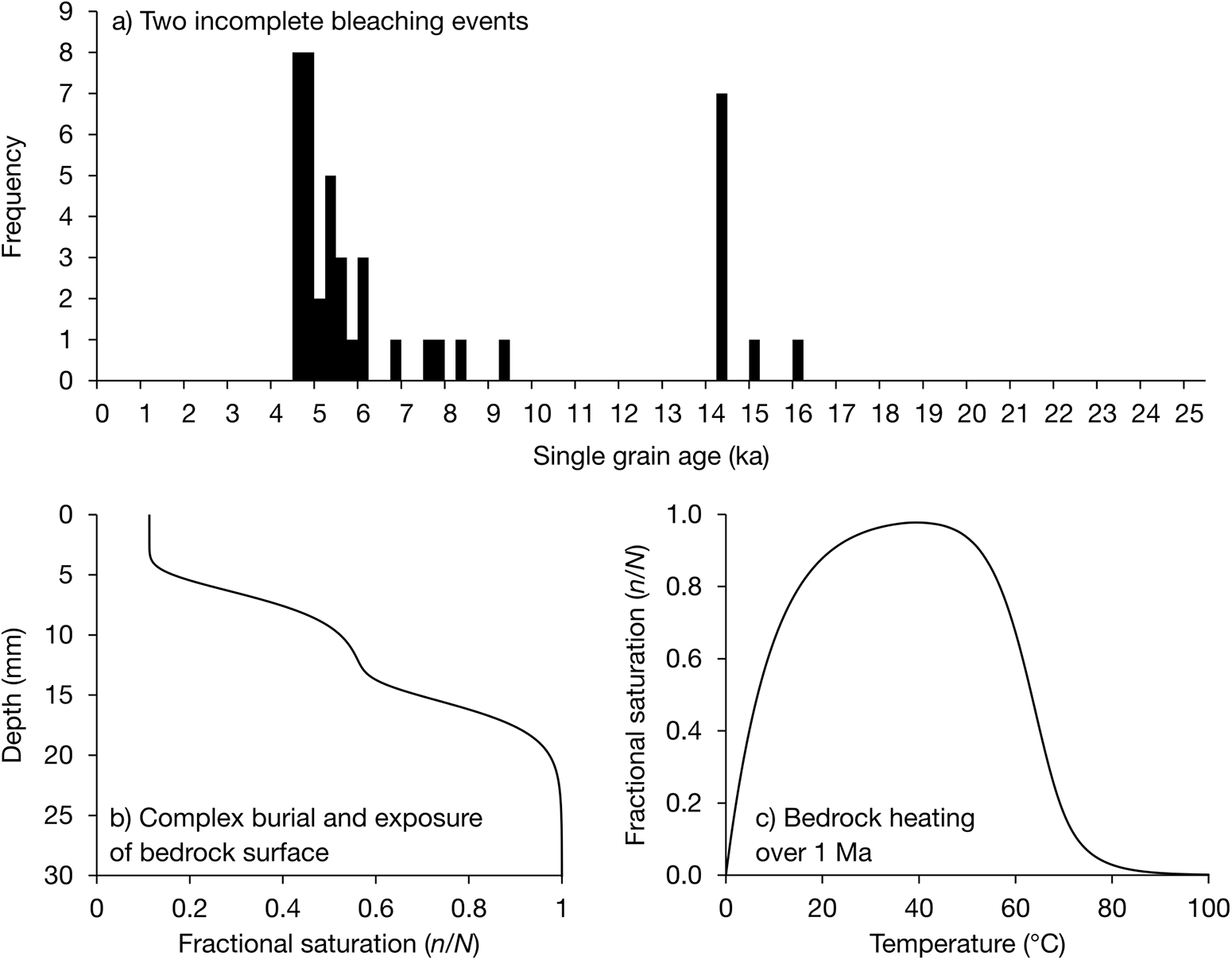
Table 2 details three applications of LuSS to simulate published datasets. In the first application, single grains of K-feldspar are exposed to sunlight for 5 h, buried for 10 ka, exposed for 3 h, then buried for another 3 ka. Both sunlight exposure events only affect some grains, as the probabilities of exposure are 1 × 10⁻⁵ and 5 × 10⁻⁵ s⁻¹, respectively. The resulting distribution (Fig. 7a) resembles the single grain ages from an alluvial fan in southern California shown in fig. 4 of Goehring et al. (Reference Goehring, Brown, Moon and Blisniuk2021). This illustrates how incomplete bleaching over multiple depositional cycles could manifest as a multimodal age distribution. To extend this application, users could investigate the relative importance of bleaching duration, sample bleaching rate, or grain exposure probability on the resulting age distribution, by adjusting these parameters individually.

Figure 7. Simulated luminescence responses for the three geologic scenarios detailed in Table 2. (a) Apparent single grain age distribution following two cycles of sunlight exposure and burial, where only some of the grains are exposed to sunlight. These results resemble those in figure 4 of Goehring et al. (Reference Goehring, Brown, Moon and Blisniuk2021). (b) The luminescence depth profile of a bedrock surface exposed to 5 ka of sunlight, buried for 30 ka, exposed to sunlight again for 20 a, then buried for 5 ka. Based on figure 1 of Brown (Reference Brown and Elias2024). (c) Fractional saturation for a quartz grain experiencing linear heating from 0°C to 100°C over 1 Ma. This represents the thermochronology result in figure 3a of Guralnik et al. (Reference Guralnik2015a).

Table 2. Three examples of using LuSS to simulate geologic scenarios.

The next example mimics fig. 1 of Brown (Reference Brown and Elias2024). A bedrock surface is exposed to sunlight for 5 ka, buried for 30 ka, exposed for 20 a, then buried for 4 ka. The resulting luminescence depth profile is shown in Fig. 7b. Here also, the user can tweak various parameters like rock opacity or the duration of bleaching events to do simplistic sensitivity analysis.

For the third example, a quartz grain is heated linearly, from 0°C to 100°C, over 1 Ma. The resulting fractional saturation history is shown in Fig. 7c, and reproduces the heating curve in fig. 3a of Guralnik et al. (Reference Guralnik2015a). Changing the trap depth, heating rate, heating linearity or final temperature would produce observably different histories. Other geologic scenarios that could readily be modeled are suggested in Brown (Reference Brown2020).

Limitations

A key limitation of LuSS is that anomalous fading is not simulated, despite the fact that many natural feldspar signals are observed to fade, meaning that a laboratory-induced signal will decay measurably on short timescales (Huntley and Lamothe, Reference Huntley and Lamothe2001). A fading sample that is irradiated at a typical laboratory dose rate will yield a larger sensitivity-normalized luminescence response for a given dose than that same sample irradiated at a geologic dose rate. This effect requires a critically important correction when estimating burial ages, as the natural signal is induced by a natural dose rate but the laboratory signals are induced by a dose rate that is many orders of magnitude greater. For example, a typical natural dose rate is several Gy/ka and the dose rates on most automated luminescence readers are on the order of 0.1 Gy/s, greater by a factor of more than 10⁹. But this effect matters less for simulating a geologic history, where the natural dose rate is not likely to change dramatically. Anomalous fading is not currently simulated in LuSS due to the added complexity and computational cost. To monitor fading by nearest neighbor recombination (Huntley, Reference Huntley2006), which is the conventional interpretation of the process (Kars et al., Reference Kars, Wallinga and Cohen2008), one must integrate over time, depth (in the case of cobbles), and also recombination distance. Likewise, the thermal decay behavior of feldspars is not included, as there are many competing and computationally intensive interpretations for these kinetics (Jain and Ankjaergaard, Reference Jain and Ankjaergaard2011; Guralnik et al., Reference Guralnik2015b).

Other important features that cannot be modeled with LuSS include the luminescence sensitivity variation among grains (Rhodes, Reference Rhodes2007) or grain-specific dose rates (Nathan et al., Reference Nathan, Thomas, Jain, Murray and Rhodes2003; Smedley et al., Reference Smedley, Duller, Pearce and Roberts2012). Nor can the user investigate significant controls on the geologic dose rate, like moisture content, overburden thickness, or disequilibrium in the ²³⁸U decay chain (Olley et al., Reference Olley, Pietsch and Roberts2004). These are simplifications that prioritize user friendliness but obscure the importance of these variables.