


1. Introduction
Perhaps the most striking manifestation of the Leidenfrost effect, named after the publication of De Aquae Communis Nonnullis Qualitatibus Tractatus by J.G. Leidenfrost, see Leidenfrost (Reference Leidenfrost1966), is the nearly frictionless motion experienced by a drop when it is placed on a sufficiently heated substrate. The reason for this behaviour lies in the fact that, when the solid temperature is high enough, the drop floats on its own vapour. Once a vapour layer is formed, the vapour lubricates the solid–liquid contact. Such a drop can take tens of seconds to evaporate (Quéré Reference Quéré2013) because the small heat conductivity of the gas limits the heat flux from the wall. The insulating effect of the vapour negatively affects the cooling of electronic or optical devices and of different materials, such as the fuel rods in nuclear plants, causing the so-called burnout phenomenon in spray cooling applications (van Limbeek et al. Reference van Limbeek, Hoefnagels, Sun and Lohse2017). On the positive side, it has been recently suggested that new lab on a chip technologies could emerge taking advantage of the increased mobility of Leidenfrost drops, which, however, would need to be controlled by appropriately patterning the substrate (Linke et al. Reference Linke, Alemán, Melling, Taormina, Francis, Dow-Hygelund, Narayanan, Taylor and Stout2006; Cousins et al. Reference Cousins, Goldstein, Jaworski and Pesci2012; Sobac et al. Reference Sobac, Rednikov, Dorbolo and Colinet2014).
Though three centuries have already passed since the Leidenfrost effect was originally reported, the description and quantification of the phenomenon is still a matter of active research. In the case the drop approaches the heated wall with a negligible velocity, different experimental and theoretical studies have been devoted to predict the thickness of the insulating vapour layer formed beneath the liquid (Burton et al. Reference Burton, Sharpe, van der Veen, Franco and Nagel2012; Sobac et al. Reference Sobac, Rednikov, Dorbolo and Colinet2014) as well as the dynamics of the spontaneous oscillations experienced by the levitating drop (Ma & Burton Reference Ma and Burton2018). Also, very recently, Zhao & Patankar (Reference Zhao and Patankar2020) have modelled the minimum Leidenfrost temperature, which has been shown to exhibit a hysteretic behaviour (Chantelot & Lohse Reference Chantelot and Lohse2021; Harvey, Harper & Burton Reference Harvey, Harper and Burton2021).
Drops usually impact the substrate with a finite velocity and, therefore, it is necessary to know how the so-called dynamic Leidenfrost temperature,  $T_L$, depends on the impact velocity (Tran et al. Reference Tran, Staat, Prosperetti, Sun and Lohse2012, Reference Tran, Staat, Susarrey-Arce, Foertsch, van Houselt, Gardeniers, Prosperetti, Lohse and Sun2013). For values of the substrate temperature
  $T_s>T_L$, the liquid–solid contact is prevented, largely reducing the heat flux and the cooling capacity of the liquid, causing the undesired burnout phenomenon mentioned above. It is known that
  $T_L$ depends on the thermo-physical properties of the liquid and the substrate, on the surrounding atmospheric conditions and also on the radius
  $R$ and velocity
  $U$ at which a drop impacts the solid (Tran et al. Reference Tran, Staat, Prosperetti, Sun and Lohse2012, Reference Tran, Staat, Susarrey-Arce, Foertsch, van Houselt, Gardeniers, Prosperetti, Lohse and Sun2013; van Limbeek et al. Reference van Limbeek, Shirota, Sleutel, Sun, Prosperetti and Lohse2016; Shirota et al. Reference Shirota, van Limbeek, Sun, Prosperetti and Lohse2016; van Limbeek et al. Reference van Limbeek, Hoefnagels, Sun and Lohse2017). Due to the number of physical and technological applications for which drops impacting in the dynamical Leidenfrost regime are relevant, numerous experimental studies have appeared in the literature reporting the value of
  $T_L$ for different types of liquids and substrates, but still there is not any available theory to reliably predict the conditions under which a drop impacting a heated substrate generates vapour enough to prevent the liquid to contact the substrate and then reduce the heat flux between the solid and the liquid. Then, a crucial step to calculate
  $T_L$ is to predict the minimum thickness or neck thickness,
  $h_m$, of the vapour film on which the drop floats when the substrate is superheated above the dynamic Leidenfrost temperature. In this contribution we present a physical model based on the classical viscous lubrication theory and on the previous results by Riboux & Gordillo (Reference Riboux and Gordillo2014), which is in good agreement with the experimental measurements of
  $h_m$ reported by de Ruiter et al. (Reference de Ruiter, Oh, van den Ende and Mugele2012) for the case of isothermal substrates and by Chantelot & Lohse (Reference Chantelot and Lohse2021) for the case of superheated substrates. In addition, using mass conservation arguments, we also deduce an equation for the minimum substrate temperature which is needed to prevent the contact between the solid and liquid at the centre of the drop: the temperature deduced in this way is in good agreement with the Leidenfrost temperatures reported by Shirota et al. (Reference Shirota, van Limbeek, Sun, Prosperetti and Lohse2016) on smooth substrates, and conclude that this equation can be used as a starting point to prevent the undesired burnout phenomenon in heat transfer applications once the effect of roughness is included in the analysis (Kim et al. Reference Kim, Truong, Buongiorno and Hu2011).
The paper is structured as follows. With the purpose of deducing an equation for  $h_m/R$, § 2 presents a model based on the results in Riboux & Gordillo (Reference Riboux and Gordillo2014), now coupled with the classical viscous lubrication equations describing the gas flow at the thin film separating the liquid from the wall. Once the equation for
  $h_m/R$ is validated by comparing the predictions with experiments, we also deduce an equation for the minimum substrate temperature which is needed to prevent the solid–liquid contact at the central part of the drop. The values of the substrate temperature provided by this equation are also compared with the dynamic Leidenfrost temperatures reported by Shirota et al. (Reference Shirota, van Limbeek, Sun, Prosperetti and Lohse2016), finding good agreement between predictions and measurements. Finally, § 3 summarizes the main results obtained in this contribution.
2. Modelling the minimum film thickness and the dynamic Leidenfrost temperature
The sketch in figure 1 shows a drop of radius  $R$ of a liquid with a density
  $\rho _l$, viscosity
  $\eta _l$, interfacial tension coefficient
  $\gamma$ and latent heat of vaporization
  $\mathcal {L}$, impacting with a velocity
  $U$ on a wall with a temperature
  $T_s$ which could be either
  $T_s=T_a$ with
  $T_a$ the surrounding gaseous atmosphere (isothermal substrate) or
  $T_s>T_b$ (superheated substrate), with
  $T_b>T_a$ indicating the liquid boiling temperature at the pressure
  $P_a$. The material properties of the surrounding atmospheric gas and of the vapour will be differentiated by means of the subscripts
  $a$ and
  $v$: the viscosity and density of these two different gases will be respectively denoted, in what follows, as
  $\eta _{(a,v)}$ and
  $\rho _{(a,v)}$; the subscript
  $l$ will be used to denote liquid quantities. From now on, the mechanical variables will be made dimensionless using
  $R$,
$R$,  $U$ and
  $\rho _l U^{2}$ and
 \begin{equation} \tau=t \frac{U}{R}, \end{equation}
will indicate the dimensionless time, with the origin of times set at the instant the drop would contact the substrate if the gas was not present. The results will be expressed in terms of the Reynolds, Stokes, Weber and Prandtl numbers,
 \begin{equation} Re=\frac{U R}{\nu_l}, \quad St=\frac{\rho_l U R}{\eta_a}, \quad We=\frac{\rho_l U^{2} R}{\gamma}, \quad Pr=\frac{\nu_l}{\alpha_l},\end{equation}
with  $\nu _l$ and
  $\alpha _l$ indicating the liquid kinematic viscosity and the heat diffusivity, and also on the dimensionless parameters
 \begin{equation} \beta=\frac{k_v(T_s-T_b)}{\eta_v\mathcal{L}}= \frac{k_v{\rm \Delta} T}{\eta_v\mathcal{L}},\quad \beta_a=\frac{k_v(T_b-T_a)}{\eta_v\mathcal{L}},\end{equation}
with  $k_v$ and
  $\eta _v$ the vapour thermal conductivity and viscosity, and with
  ${\rm \Delta} T=T_s-T_b$ indicating the value of the superheat.
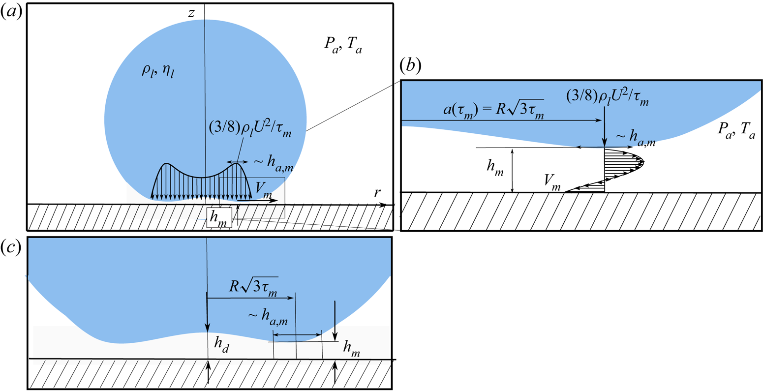
(a) Sketch of the impact of a drop of radius  $R$ and velocity
  $U$ in the presence of air. As the drop approaches the wall, the dimple of height
  $h_d$ – see also (c) – forms at the dimensionless instant
  $t_m U/R = \tau _{m} \ll 1$ and the neck, located at
  $r=R\sqrt {3\tau _m}$, skates with a velocity
  $V_m=V(\tau _m)$ over a thin air film that either delays or prevents contact. This figure also shows the pressure distribution at the bottom of the impacting drop when the minimum air film thickness
  $h_{m}$ is reached at
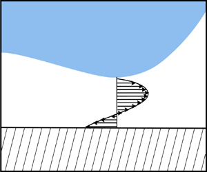
  $\tau _m$. (b) The pressure difference
 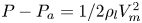 $P-P_a=1/2\rho _l V^{2}_m$ in a region of width
  $h_{a,m}$ and the relative motion between the neck and the wall induce the sketched Poiseuille and Couette flows, which are represented in a frame of reference moving with the neck velocity
  $V_m$; see (2.10)–(2.13). (c) The sketch illustrates the characteristic geometry of the entrapped bubble, which possesses a thickness
  $h_d$ at the axis of symmetry and a thickness
  $h_m\ll h_d$ at a distance
  $a(\tau _m)=R\sqrt {3\tau _m}$ from the axis of symmetry.
As a previous step for our subsequent developments, we first review the results obtained by Riboux & Gordillo (Reference Riboux and Gordillo2014, Reference Riboux and Gordillo2017) (hereafter referred to as R&G) which will also be used to analyse those cases of interest here in which a gas layer is entrapped between a falling drop and the wall.
Indeed, with the purpose of analysing the impact of an axisymmetric drop over an impermeable wall, R&G made use of Wagner's theoretical framework (Wagner Reference Wagner1932), which was originally envisaged to describe the impact of two-dimensional solids with a small deadrise angle over a gas–liquid interface. The time evolution of the wetted radius  $a(t)$ was determined in Riboux & Gordillo (Reference Riboux and Gordillo2014) by means of the so-called Wagner condition (Wagner Reference Wagner1932; Korobkin & Pukhnachov Reference Korobkin and Pukhnachov1988); see Appendix A for further details. Indeed, this was done by introducing the velocity field given in (2) of the supplementary material (SM) of Riboux & Gordillo (Reference Riboux and Gordillo2014), which satisfies the Laplace equation as well as the impenetrability condition on a disc of radius
  $a(t)$, into (3) of the same SM, which expresses the Wagner condition corresponding to a spherical drop of radius
  $R$ impacting against a solid with a velocity
  $U$. The solution of (3) in the SM of Riboux & Gordillo (Reference Riboux and Gordillo2014), see also Appendix A, provides with the following expression for the wetted radius:
 \begin{equation} a(t) = \sqrt{3URt} = R\sqrt{3\tau} \end{equation}
(see figure 1). Since the present study focuses on the analysis of the impact of a drop that entraps air or vapour between the falling liquid and the wall, a natural question that arises is whether (2.4) will still be valid or not when a thin gas film is entrapped. The answer is that, provided that the vertical velocity  $\partial h/\partial t$ of the slender and thin gas layer of thickness
  $h(r,t)$ such that
  $h(r,t)/a(t)\ll 1$ verifies the condition
  $(1/U)\partial h/\partial t\ll 1$, the velocity field in (2) of the SM in Riboux & Gordillo (Reference Riboux and Gordillo2014) will contain only relative errors of order
  $\sim (1/U) \partial h/\partial t\ll 1$ and, therefore, the expression for
  $a(t)$ in (2.4) is expected to accurately describe the drop impact process also when the drop spreads over a thin air or vapour layer. The experimental results reported by Chantelot & Lohse (Reference Chantelot and Lohse2021) in their figure 4(b) confirm that
  $(1/U)\partial h/\partial t\ll 1$ and, therefore, it is expected that the wetted radius, also in the physical situation of interest here, can be calculated using (2.4), a prediction which is indeed confirmed by the experimental results in Shirota et al. (Reference Shirota, van Limbeek, Sun, Prosperetti and Lohse2016), Chantelot & Lohse (Reference Chantelot and Lohse2021).
Therefore, we can make use here of the same theoretical framework as that used in R&G, where local mass and momentum balances were applied in a frame of reference moving with the velocity  $V(t)$ at which the liquid wets the substrate,
 \begin{equation} V(t) = \frac{{{\rm d}}a}{{{\rm d}}t}=U\frac{\sqrt{3}}{2}\tau^{{-}1/2}, \end{equation}
since these balances provide us with the following equation for the thickness of the thin lamella:
 \begin{equation} h_a(t) = R \frac{\sqrt{12}}{3{\rm \pi}}\tau^{3/2}, \end{equation}
which is ejected radially outwards from  $r=a(t)$ for
  $t>t_e$, with
  $t_e U/R\ll 1$ the ejection time.
When expressed in the frame of reference moving with a velocity  $V(t)$, the local velocity field in R&G also reveals the existence of a stagnation point of the flow located at a distance
  $\sim h_a(t)$ upstream of
  $r=a(t)$; see figure 1 and Appendix A. At this location, the liquid pressure is maximum and, since the local flow is quasi-steady, the Euler–Bernoulli equation provides the following expression for the pressure jump:
 \begin{equation} {\rm \Delta} p(t)=P_l(r \simeq a(t)) - P_a =\tfrac{1}{2}\rho_l V(t)^{2}=\tfrac{3}{8}\rho_l U^{2} \tau^{{-}1}. \end{equation}
Here use of (2.5) has been made. For our subsequent purposes, it also proves convenient to point out here that the combination of (2.7) and (2.6) reveals that the maximum pressure gradient at the liquid side, which is reached at  $r\simeq a(t)$, can be approximated as
 \begin{equation} \sim \frac{{\rm \Delta} p(t)}{h_a(t)}=\frac{\rho_l U^{2}}{R} \frac{9{\rm \pi}}{16\sqrt{3}} \tau^{{-}5/2} . \end{equation}
 Since the maximum pressure diverges as  $\tau ^{-1}$ for
  $\tau \rightarrow 0$, see (2.7), the maximum attainable pressure during the drop impact process and, hence, the minimum thickness
  $h_m$, are reached at the characteristic dimple formation time,
  $h_d/U$, with
  $h_d$ the height of the entrapped central bubble, which depends on
  $St$ as (Mandre, Mani & Brenner Reference Mandre, Mani and Brenner2009; Bouwhuis et al. Reference Bouwhuis, van der Veen, Tran, Keij, Winkels, Peters, van der Meer, Sun, Snoeijer and Lohse2012; Chantelot & Lohse Reference Chantelot and Lohse2021)
 \begin{equation} h_d\simeq 2.8 R St^{{-}2/3} .\end{equation}
 Therefore, the dimensionless instant  $\tau _{m}$ at which
  $h_{m}$ is reached can be well approximated by
 \begin{equation} \tau_{m}\approx C_\tau St^{{-}2/3},\quad \text{with } C_\tau\simeq 12.4,\end{equation}
a constant deduced from the analysis of the experiments in Chantelot & Lohse (Reference Chantelot and Lohse2021) and very kindly provided to us by the authors.
Then, the initial velocity at which the neck propagates radially outwards, the maximum attainable liquid pressure and also the characteristic distance along which the pressure variations in the liquid take place, see figure 1, are calculated particularizing equations (2.5)–(2.7) at  $\tau =\tau _m = C_\tau {{St}}^{-2/3}$, obtaining the following results:
 \begin{gather} V_m=V(\tau_m) = U\frac{\sqrt{3}}{2} C^{{-}1/2}_\tau St^{1/3} , \end{gather}
 \begin{gather}{\rm \Delta} p_m={\rm \Delta} p(\tau_m)=\frac{3}{8C_\tau}\rho_lU^{2} St^{2/3}, \end{gather}
 \begin{gather}h_{a,m}=h_a(\tau_m) = R \frac{\sqrt{12C_\tau^{3}}}{3{\rm \pi}} St^{{-}1} . \end{gather}
 Making use of (2.10)–(2.13) and of the results in R&G, we can now proceed and provide a scaling of  $h_{m}$ as a function of the impact velocity.
First, in the case there is not a temperature jump between the substrate and the drop, the liquid can levitate over the solid at a distance  $h_{m}$ thanks to the physical mechanism, illustrated in figure 1, which constitutes the basis of the classical hydrodynamic lubrication theory. Indeed, note that if the drop does not contact the wall, a neck located at
  $r=R\sqrt {3\tau }$ with
  $\tau \geq \tau _{m}$ and separated a distance
  $h_{m}$ from the solid, moves radially outwards with the velocity
  $V_m$ given by (2.11), forming a small angle with the horizontal substrate. In the frame of reference moving with the velocity
  $V_m$, the Couette flow rate per unit length induced by the relative motion between the drop and the substrate,
  $V_m h_{m}/2$ with
  $V_m$ given in (2.11), is directed inwards. However, the pressure gradient at the dimple,
  ${\rm \Delta} p_m/h_{a,m}$ with the pressure difference
  ${\rm \Delta} p_m$ and
  $h_{a,m}$ respectively given by (2.12) and (2.13), induces a Poiseuille flow ensuring that mass conservation is preserved in the slightly converging geometry sketched in figure 1. Therefore, the dimple can levitate over the substrate at the distance
  $h_{m}$ given by the solution of
 \begin{equation} \frac{V_m h_m}{2}\simeq \frac{1}{h_{a,m}}\frac{h^{3}_m}{12\eta_a}\frac{\rho_l V^{2}_m}{2}\Rightarrow \frac{h^{3}_{m}}{12\eta_a}\frac{3\rho_l U^{2}}{8\tau_{m} h_{a,m}}\simeq \frac{\sqrt{3}}{4\tau^{1/2}_{m}} U h_{m}, \end{equation}
with  $\tau _{m}$ given in (2.10), yielding
 \begin{equation} \frac{h_{m}}{R}\simeq \frac{4 C_\tau}{\sqrt{\rm \pi}} St^{{-}7/6} .\end{equation}
 Note that 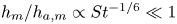 $h_m/h_{a,m}\propto St^{-1/6}\ll 1$, a fact indicating that the slightly converging geometry is indeed slender. In addition, the ratio of inertial to viscous stresses in the gas flow is such that
  $\rho _a V_m h^{2}_m/(\eta _a h_{a,m})\sim \rho _a/\rho _l\ll 1$, a fact confirming that the viscous lubrication approach can be employed to describe the gas flow in the slightly converging geometry surrounding the neck; see figure 1.
The result expressed by (2.15) has been deduced neglecting the effect of the capillary pressure. The approximation of neglecting capillary effects will be valid whenever the characteristic capillary length  $\ell _c$, which we define here as
 \begin{equation} \frac{\gamma h_m}{\ell^{2}_c}\sim {\rm \Delta} p_m\Rightarrow \ell_c\sim \sqrt{\frac{\gamma h_m}{{\rm \Delta} p_m}}=\sqrt{\frac{8 C_\tau}{3}}\sqrt{R h_{m}} We^{{-}1/2} St^{{-}1/3}, \end{equation}
with  ${\rm \Delta} p_m$ given in (2.12), verifies the condition
 \begin{equation} \frac{h_{a,m}}{\ell_c}\gtrsim 1 .\end{equation}
In order to find the condition expressing the crossover between the inertial and capillary dominated regimes, which takes place when  $h_{a,m}/\ell _c\sim 1$, we make use of (2.13) and (2.16) and also the result in (2.15),
  $h_m\propto St^{-7/6}$, finding that
 \begin{equation} \frac{h_{a,m}}{\ell_c}\sim We^{1/2} St^{{-}1/12} .\end{equation}
Using the result in (2.18), we conclude that capillary effects will be relevant only if
 \begin{equation} h_{a,m}\lesssim \ell_c\Rightarrow We St^{{-}1/6}\lesssim 1.\end{equation}
In the capillary dominated regime, namely when condition (2.19) is satisfied, the characteristic length scale where pressure variations take place is not  $h_{a,m}$ but
  $\ell _c$ defined in (2.16). Making use of (2.16), the expression for the minimum film thickness in the capillary dominated regime is
 \begin{equation} \frac{V_m h_m}{2}\simeq \frac{1}{\ell_c}\frac{h^{3}_m}{12\eta_a}\frac{\rho_l V^{2}_m}{2}\Rightarrow \frac{h_m}{R}\simeq 8 C^{2/3}_\tau We^{{-}1/3} St^{{-}10/9} .\end{equation}
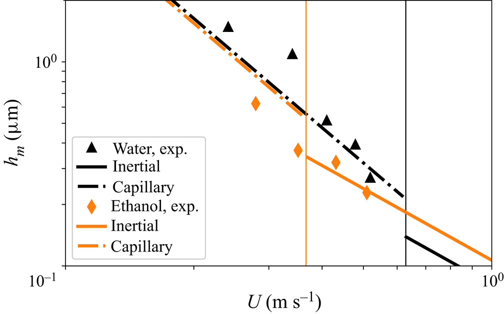
 The inertial and capillary scalings for  $h_{m}$ respectively given in (2.15) and (2.20), are compared in figure 2 with the experimental data in de Ruiter et al. (Reference de Ruiter, Oh, van den Ende and Mugele2012). In this figure the vertical lines indicate the values of the impact velocities for which
  $We St^{-1/6}=1$, this being the approximate condition expressing the transition from the capillary,
  $We St^{-1/6}\lesssim 1$, to the inertial,
  $We St^{-1/6}\gtrsim 1$, regime; see (2.18) and (2.19). Due to the fact that the range of experimental values of
  $U$ in figure 2 is quite limited, Appendix B considers the case in which the transition between inertial and capillary regimes took place for a value
  $We St^{-1/6}=C$ with
  $C>1$ a value such that all the experiments laid within the capillary regime. In contrast with the results depicted in figure 2, the results in Appendix B reveal that the experimental data corresponding to both ethanol and water cannot be reproduced simultaneously by the capillary scaling given in (2.20), a result which further confirms that the value of
  $h_{m}$ can be calculated by means of (2.15) with small relative errors if
  $We St^{-1/6}\gtrsim 1$. Therefore, since most of the available experimental data correspond to impact velocities for which this condition is satisfied, the pressure gradient at the neck can be calculated, in most cases of practical interest, using the expression
  ${\rm \Delta} p_m/h_{a,m}$ with
  ${\rm \Delta} p_m$ and
  $h_{a,m}$ given respectively by (2.12) and (2.13).
Comparison of the predictions given in (2.15) and (2.20) with the experimental data in figure 3(a) in de Ruiter et al. (Reference de Ruiter, Oh, van den Ende and Mugele2012), where  $R=1.05\times 10^{-3}$ m,
  $\rho _{water}=1000\ \text {kg}\ \text {m}^{-3}$,
  $\rho _{ethanol}=789$ kg
 $\text {m}^{-3}$,
 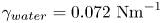 $\gamma _{water}=0.072\ \text {Nm}^{-1}$,
  $\gamma _{ethanol}=0.022\ \text {Nm}^{-1}$,
  $\eta _{water}=10^{-3}\ \text {Pa} \cdot \text {s}$,
  $\eta _{ethanol}=1.07\times 10^{-3}\ \text {Pa} \cdot \text {s}$ and
  $\eta _{a}=1.8\times 10^{-5}\ \text {Pa} \cdot \text {s}$. The measurements in de Ruiter et al. (Reference de Ruiter, Oh, van den Ende and Mugele2012) provide
  $h_{m}(U)$ for two different liquids, ethanol (orange diamonds) and water (black triangles); we do not include the experimental data corresponding to
  $CaCl_2$ since the precise values of the material properties of that liquid were not provided in the original work. The black and orange vertical lines indicate the velocity
  $U$ for which
  $We St^{-1/6}=1$ for each of the two liquids. Continuous/dashed lines represent the inertial/capillary regimes calculated using either (2.15) or (2.20) for the value
  $C_\tau =12.4$ provided by Chantelot & Lohse (Reference Chantelot and Lohse2021) and, therefore, with no adjustable constants.
Let us point out here to the fact, depicted in figure 2, that the values of  $h_m$ can be similar to the mean free path of the gas, which for the case of air at normal conditions is
  $\sim 100$ nm. Therefore, the classical expressions of the Couette and Poiseuille gas flow rates used above, which are deduced imposing the no-slip boundary condition at both the wall and the gas–liquid interface, should be slightly modified taking into account the effect of the slip length at the top and bottom boundaries limiting the gas flow. Since these corrections lead to a more complex expression for the gas flow rate, which would then depend on the mean free path of the gas (see e.g. the SM of (Riboux & Gordillo Reference Riboux and Gordillo2014)) and in view of the fair agreement between predictions and measurements depicted in figure 2, in this contribution we simplify the analysis and assume that the slip length is zero, enabling us to make use of the classical and well-known expressions for the Couette and Poiseuille flow rates used, for instance, in (2.14).
We now want to consider the case of drops in the Leidenfrost regime impacting over superheated substrates and it is our aim here to determine how  $h_m$ depends on the different control parameters. The only essential difference with respect to the case of isothermal substrates is that, in order to avoid the liquid–solid contact, the vapour produced at the evaporating interface needs to flow beneath the region where the minimum distance to the wall is attained. The equation deduced using this physical idea will provide us with an equation expressing
  $h_m$ as a function of
  $U$, of the superheat
 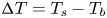 ${\rm \Delta} T=T_s-T_b$ and of the material properties of the liquid, gas and vapour. Indeed, it has been extensively reported that the thermal conductivity and thermal diffusion coefficient of the solid largely affects the dynamical Leidenfrost temperature (van Limbeek et al. Reference van Limbeek, Shirota, Sleutel, Sun, Prosperetti and Lohse2016; van Limbeek et al. Reference van Limbeek, Hoefnagels, Sun and Lohse2017), but in this contribution we focus on the case of solids with a very high conductivity such as metals or sapphire so that the substrate temperature is constant throughout the process.
We first make use of the approximation in Sobac et al. (Reference Sobac, Rednikov, Dorbolo and Colinet2014), where the heat power per unit area which is transferred from the heated wall to the evaporating interface is given by
 \begin{equation} k_v\frac{{\rm \Delta} T}{h_m} .\end{equation}
Therefore, if the heat flux across the liquid thermal boundary layer is neglected (see Appendix C for details), the flow rate of vapour per unit length which is produced along a length  $h_{a,m}$ is (Sobac et al. Reference Sobac, Rednikov, Dorbolo and Colinet2014)
 \begin{equation} q_v=k_v\frac{{\rm \Delta} T}{\rho_v \mathcal{L}}\frac{h_{a,m}}{h_m}.\end{equation}
Consequently, the ratio of inertial to viscous stresses describing the flow of vapour produced downstream of the stagnation point along a length  $h_{a,m}$ is given by
 \begin{equation} \frac{\rho_v q_v h_m}{\eta_v h_{a,m}}=\beta, \end{equation}
with  $\beta$ defined in (2.3a,b). The values of the superheat
  ${\rm \Delta} T$ considered here are such that
  $\beta <1$ and, therefore, we can safely resort to the viscous lubrication approach to describe the flow of vapour in the region of length
  $h_{a,m}$ located downstream of the stagnation point, and can also make use of (2.22) to calculate the flow rate of vapour per unit length produced in this small region.
Analogously to the case of isothermal substrates, the value of  $h_m/R$ is deduced from the mass balance
 \begin{equation} \frac{V_m h_m}{2}+\frac{1}{h_{a,m}}\frac{h^{3}_m}{12\eta_v}\frac{\rho_l V^{2}_m}{2}\simeq q_v, \end{equation}
with  $q_v$ given in (2.22).
The substitution of (2.11)–(2.13) into (2.24) yields the equation for  $h_m/R$,
 \begin{equation} y\left(1+y\frac{\eta_a}{6\eta_v}\right)=\beta^{*}, \end{equation}
with
 \begin{equation} y=\frac{3{\rm \pi}}{8 C^{2}_\tau} St^{7/3} \left(\frac{h_m}{R}\right)^{2} \quad\text{and}\quad \beta^{*} =\beta\left(\frac{\rho_l}{\rho_v}\right) \left(\frac{\eta_v}{\eta_a}\right),\quad\text{with } \beta=\frac{k_v{\rm \Delta} T}{\eta_v\mathcal{L}},\end{equation}
and whose solution provides the following expression for  $h_m/R$:
 \begin{equation} \frac{h_m}{R}=C_\tau\sqrt{\frac{8}{3{\rm \pi}}}St^{{-}7/6} [3(\eta_v/\eta_a)\sqrt{1+2(\eta_a/\eta_v)\beta^{*}/3}-3 (\eta_v/\eta_a)]^{1/2}.\end{equation}
 Here we could use  $C_\tau =12.4$ as done in the isothermal case but choose to introduce a slight correction to this value. Indeed, the result
  $\tau _m\propto h_d/R=C_\tau St^{-2/3}$ was deduced in Mandre et al. (Reference Mandre, Mani and Brenner2009), Bouwhuis et al. (Reference Bouwhuis, van der Veen, Tran, Keij, Winkels, Peters, van der Meer, Sun, Snoeijer and Lohse2012) using the mass balance at the dimple which, using the viscous lubrication approach, reads as
 \begin{equation} U\sqrt{R h_d}\sim \frac{h^{3}_d}{12 \eta_a}\frac{{\rm \Delta} p_{dimple}}{\sqrt{R h_d}}\Rightarrow h_d/R\propto St^{{-}2/3} .\end{equation}
Equation (2.28) has been deduced taking into account that the thickness and width of the dimple are respectively given by  $h_d$ and
  $\sqrt {R h_d}$ and also that the liquid pressure at the axis of symmetry is (Bouwhuis et al. Reference Bouwhuis, van der Veen, Tran, Keij, Winkels, Peters, van der Meer, Sun, Snoeijer and Lohse2012)
  ${\rm \Delta} p_{dimple}\sim \rho _l \partial \phi /\partial t\sim \rho _l U^{2}\sqrt {R h_d}/h_d$, with
  $\phi$ the liquid velocity potential. For the case at hand, in which vapour is produced at the dimple, the term on the left-hand side of (2.28) has to be replaced by
  $\sqrt {Rh_d}(U+k_v{\rm \Delta} T/(\rho _v h_d\mathcal {L}))$. Therefore, expressing
 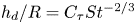 $h_d/R=C_\tau St^{-2/3}$, the balance (2.28) yields the equation for
  $C_\tau$,
 \begin{equation} C^{5/2}_\tau=12.4^{3/2}(C_\tau+\beta^{*}St^{{-}1/3}), \end{equation}
where the prefactor has been chosen in order to recover the one for isothermal substrates and  $\beta ^{*}$ is defined in (2.26a,b). The prediction in (2.27)–(2.29), where the material properties of the vapour and air are calculated as a function of temperature as it is detailed in Appendix D, is compared in figure 3 with the experimental data in figure 4(e) of Chantelot & Lohse (Reference Chantelot and Lohse2021), where
 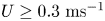 $U\geq 0.3\ \text {ms}^{-1}$ and, therefore, capillary effects can be neglected; see figure 2 and (2.19). In figure 3 the ratio
  $h_{CL}/h_{th}$ between experimental measurements (
 $h_{CL}$) and the values of
  $h_m$ calculated using (2.27) for the value of
  $C_\tau$ predicted by (2.29), (
 $h_{th}$), are very close to 1, a fact supporting the validity of our description. Let us point out that the same good agreement as that depicted in figure 3 is obtained if instead of calculating
  $C_\tau$ through (2.29), we make use of the isothermal value
  $C_\tau =12.4$.
Comparison between the experimental measurements in Chantelot & Lohse (Reference Chantelot and Lohse2021) and our prediction in (2.27) using the value of  $C_\tau$ given by the solution of (2.29) and the values of the material properties given in Appendix D.
As a further check of our result, we represent in figure 4 the value of the substrate temperature calculated using (2.25)–(2.26a,b) for three given values of  $h_m$. The values of
  $h_m$ in figure 4 are not arbitrary, but represent the most likely values of the surface asperities or of the interfacial contaminants that trigger the contact between the solid and the wall at the neck region; see figure 9(d) of Chantelot & Lohse (Reference Chantelot and Lohse2021). Our predictions are compared in figure 4 with the experimental data in Chantelot & Lohse (Reference Chantelot and Lohse2021) and Lee et al. (Reference Lee, Harth, Rump, Kim, Lohse, Fezzaa and Je2020) where the authors provide the values of the critical temperature above which the Leidenfrost effect is observed for a given impact speed. The results depicted in figure 4 reveal that the calculated values are similar to experimental ones within the characteristic range of values of
  $h_m$ given in figure 9(d) of Chantelot & Lohse (Reference Chantelot and Lohse2021). Clearly, the larger the size of the impurity, or, equivalently, of
  $h_m$, the larger the substrate temperature needs to be to prevent contact with the solid, this conclusion being analogous to the previous findings by Kim et al. (Reference Kim, DeWitt, McKrell, Buongiorno and Hu2009, Reference Kim, Truong, Buongiorno and Hu2011), who found that the presence of particles or the use of porous substrates favour the contact between the liquid and the solid. Note also in figure 4 that the differences between the values of the temperature reported by Chantelot & Lohse (Reference Chantelot and Lohse2021) and those reported by Lee et al. (Reference Lee, Harth, Rump, Kim, Lohse, Fezzaa and Je2020) are likely caused by the different type of set-up used and also because of the different sizes of the impurities present in each of the two experiments.
The values of the substrate temperature calculated through (2.25) and (2.26a,b) within the range of values of  $h_m$ provided in figure 9(d) of Chantelot & Lohse (Reference Chantelot and Lohse2021) are compared in this figure with the experimental data reported by Chantelot & Lohse (Reference Chantelot and Lohse2021) in their figure 5(a) (red diamonds indicate short-time contact) and Lee et al. (Reference Lee, Harth, Rump, Kim, Lohse, Fezzaa and Je2020) (black dots indicate short-time contact). For a given impact speed, short-time contact is expected for smaller temperatures than those predicted by the theoretical curves, whereas no contact is expected for larger values of the substrate temperature. Given a value of
  $h_m$, the values of the substrate temperature have been calculated by means of (2.25) and (2.26a,b) using the material properties of ethanol and air given in Appendix D and using the value
  $C_\tau =12.4$. Note that the predicted values are very sensitive to the value of
  $h_m$, namely, to the size of the impurities causing the contact between the liquid and the solid at the neck region.

Finally, note that mass conservation for the vapour produced at the central dimple provides us with an equation for the minimum value of the superheat which is necessary to feed the growth of a central vapour bubble of radius  $R\sqrt {3 \tau }$ and constant thickness
  $h_d/R\simeq 2.8 St^{-2/3}$ (Shirota et al. Reference Shirota, van Limbeek, Sun, Prosperetti and Lohse2016; Chantelot & Lohse Reference Chantelot and Lohse2021) which prevents the contact between the liquid and the solid at the central part of the drop. Indeed, on the one hand, the volumetric growth rate of the vapour bubble is
 \begin{equation} 2{\rm \pi} R^{2} U \sqrt{3\tau_m}\frac{\sqrt{3}}{2\sqrt{\tau_m}} \left(\frac{h_d}{R}\right)=3\times 2.8 {\rm \pi}R^{2} U St^{{-}2/3}, \end{equation}
where use of (2.9) has been made. On the other hand, the mass flow rate of vapour produced at the dimple is
 \begin{equation} {\rm \pi}k_v\frac{{\rm \Delta} T}{h_d\mathcal{L}}(\sqrt{3R h_d})^{2} .\end{equation}
It can be easily checked (see (2.22) and (C5) and (C6) in Appendix C) that the mass flow rate of vapour produced at the neck is
 \begin{equation} \sim {\rm \pi}R k_v\frac{{\rm \Delta} T}{\mathcal{L}} St^{{-}1/6} \beta^{{-}1/4} (\rho_l/\rho_v)^{{-}1/4}(\eta_v/\eta_a)^{{-}1/2}, \end{equation}
and, thus, much smaller than the mass flow rate of vapour produced at the dimple; see (2.31). Therefore, neglecting the contribution of the vapour produced at the neck and using (2.30) and (2.31), the mass balance providing the minimum value of the superheat,  ${\rm \Delta} T_L$, for which enough vapour is produced to feed the growth of a vapour bubble at the centre of the drop is
 \begin{equation} k_v\frac{{\rm \Delta} T_L}{\eta_a\mathcal{L}}=2.8\frac{\rho_{v0}}{\rho_l} \left(\frac{273+T_b}{273+T}\right)St^{1/3}\Rightarrow {\rm \Delta} T_L=2.8 \frac{\rho_{v0}}{\rho_l}\left(\frac{273+T_b}{273+T}\right) \frac{\eta_a}{\eta_v}Pr_v\frac{\mathcal{L}}{C_{p,v}} St^{1/3}, \end{equation}
where  $Pr_{v}$ is the vapour Prandtl number,
  $C_{p,v}$ is the heat capacity of the vapour at constant pressure and
  $\rho _{v 0}\simeq 1.43$ kg
 $\text {m}^{-3}$ is the vapour density at atmospheric pressure at the boiling temperature. Note that the vapour density inside the central vapour bubble has been calculated at the temperature
  $T=(T_b+T_s)/2$ and assuming that the pressure is similar to the atmospheric one. The values of
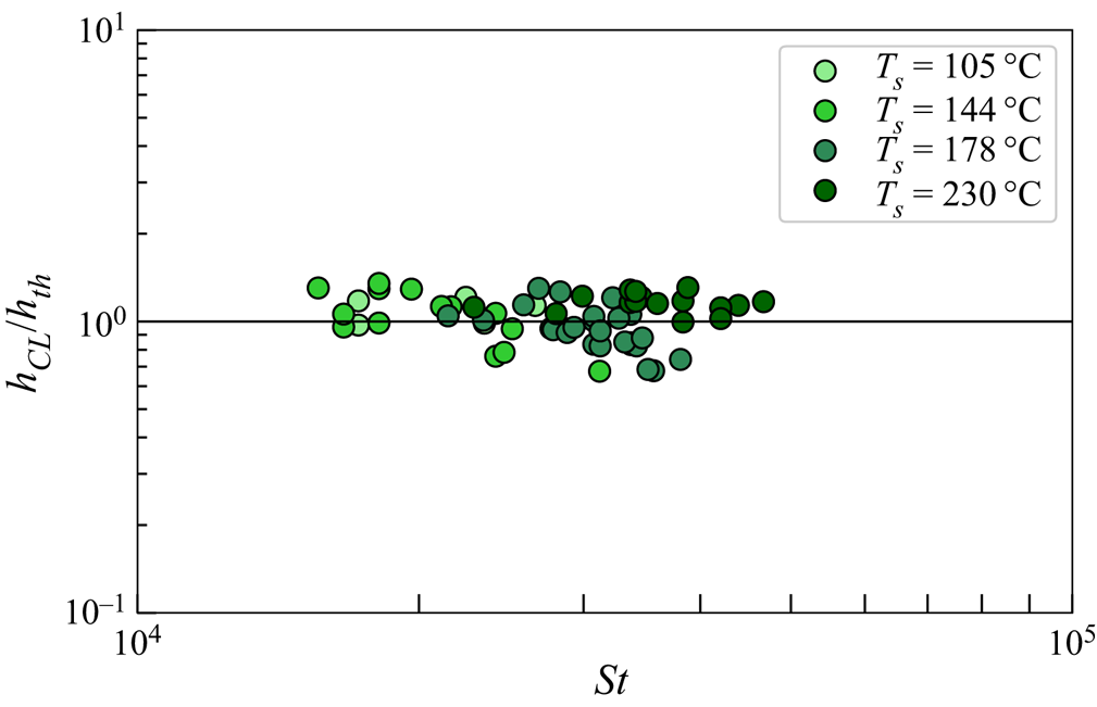
  ${\rm \Delta} T_L$ calculated through (2.33) are represented in figure 5 as a function of
  $U$ taking into account the fact that material properties depend on temperature as it is detailed in Appendix D. The calculated values of
  ${\rm \Delta} T_L$ using (2.33) are in good agreement with those reported by Shirota et al. (Reference Shirota, van Limbeek, Sun, Prosperetti and Lohse2016) and, thus, we believe that our (2.33) can be used to predict a value of the dynamic Leidenfrost temperature which is very useful for applications, i.e. the one that needs to be known in order to prevent the undesired burnout phenomenon, which occurs because the growth of the vapour bubble at the centre of the drop largely decreases the heat flux between the wall and the liquid. However, let us point out here that the validity of (2.33) is limited to those cases in which the characteristic size of surface impurities or of substrate corrugations is smaller than
  $h_d\simeq 2.8 R St^{-2/3}$; indeed, as it was discussed previously and was reported in Kim et al. (Reference Kim, DeWitt, McKrell, Buongiorno and Hu2009, Reference Kim, Truong, Buongiorno and Hu2011), the presence of surface asperities and of particles of size comparable to
  $h_d$ contribute to destabilize the vapour layer, favouring the contact between the liquid and the solid, hence increasing the Leidenfrost temperature. The results in figure 5 also show that the differences between the predicted and measured values of
  ${\rm \Delta} T_L$ are rather small for
  $U\lesssim 3$ m s
 $^{-1}$, but increase up to
  $\sim 20\,^{\circ }$C for the larger impact velocities. These differences could be attributable to the fact that (2.33) contains no fitting constants; we even make use of the value of the prefactor
  $2.8$ in
  $h_d\simeq 2.8 R St^{-2/3}$, which has been determined experimentally for smaller values of the impact velocity (Bouwhuis et al. Reference Bouwhuis, van der Veen, Tran, Keij, Winkels, Peters, van der Meer, Sun, Snoeijer and Lohse2012). In addition, the material properties of the gases are calculated in our approach at the mean temperature
  $(T_b+T_s)/2$ and our result makes use of the air viscosity in the definition of
  $St$, whereas the viscosity of the gas in the central bubble should correspond to the value of a mixture of vapour and air. In spite of the approximations made, the value of the Leidenfrost temperature calculated by means of (2.33) approximates the experimental measurements with relative errors of just
  ${\sim}15 \%$ for the larger impact speeds.
Comparison between the values of  ${\rm \Delta} T_L$ predicted by (2.33) using the material properties given in Appendix D and the values of the Leidenfrost temperature reported by Shirota et al. (Reference Shirota, van Limbeek, Sun, Prosperetti and Lohse2016) corresponding to ethanol. The horizontal black line indicates the value of
  $T_b$.
As a final remark, note that a similar mass balance to that expressed by (2.33) cannot be satisfied for the case of drops impacting over isothermal substrates. This is because the relative flow of air through the neck region will always be smaller than the rate of growth of a cylinder of constant height  $h_d$ and increasing radius
  $R\sqrt {3\tau }$, this fact explaining the rather different geometries of both the entrapped gas bubble and of the neck region seen in the experiments reported by de Ruiter et al. (Reference de Ruiter, Oh, van den Ende and Mugele2012) for the case of isothermal substrates and by Chantelot & Lohse (Reference Chantelot and Lohse2021) for the case of superheated substrates.
3. Conclusions
In this contribution we have presented a simplified physical model for the minimum thickness  $h_m$ of the vapour film that separates an impacting drop from a wall superheated above the so-called dynamic Leidenfrost temperature. By using the classical viscous lubrication approach and the results in Riboux & Gordillo (Reference Riboux and Gordillo2014), we have deduced an algebraic equation that approximates well the experimental measurements of
  $h_m$ reported by Chantelot & Lohse (Reference Chantelot and Lohse2021). Moreover, we have also provided equations for the minimum film thickness for the case drops impact over isothermal substrates and, in this case, the agreement between predictions and experimental observations by de Ruiter et al. (Reference de Ruiter, Oh, van den Ende and Mugele2012) is also good, a fact supporting the validity of our approach. Finally, we have deduced an equation for the minimum substrate temperature for which the vapour produced at the centre of the drop prevents the contact between the liquid and the solid. The values obtained using this equation with real temperature-dependent material properties of the gas and the vapour are in good agreement with those reported by Shirota et al. (Reference Shirota, van Limbeek, Sun, Prosperetti and Lohse2016) for the dynamic Leidenfrost temperature, a fact indicating that our equation for
  ${\rm \Delta} T_L$ could be used in heat transfer applications in those cases in which the characteristic size of impurities is sufficiently small when compared with the thickness of the bubble entrapped at the centre of the drop.
Acknowledgements
We are grateful to Dr P. Chantelot for sharing his published experimental data with us and to Professor D. Lohse for valuable discussions and comments on the manuscript.
Funding
This work has been supported by the Spanish Ministerio de Ciencia e Innovación under Project PID2020-115655G, partly financed through European funds.
Declaration of interest
The authors report no conflict of interest.
Appendix A. Summary of some results in Riboux & Gordillo (Reference Riboux and Gordillo2014)
In Riboux & Gordillo (Reference Riboux and Gordillo2014) we calculated the time evolution of the wetted radius  $a(\tau )$ of a spherical drop of radius
  $R$ falling with the velocity
  $-U$ over a horizontal solid substrate located at
  $z=0$ in terms of dimensionless variables defined using
  $R$,
$R$,  $U$,
$U$,  $R/U$,
  $\rho _l U^{2}$ as characteristic values of length, velocity, time and pressure, respectively; see figure 6. For that purpose, we made use of the classical ideas in potential flow aerodynamics where, thanks to the small thicknesses and slender geometries, boundary conditions are linearized around
  $z=0$. Indeed, since the Reynolds number is large, the liquid velocity field
  $\boldsymbol {v}$ is irrotational outside the thin boundary layers where viscous stresses are confined and, therefore,
  $\boldsymbol {v}=\boldsymbol {\nabla }\phi$ with
  $\phi$ indicating the velocity potential that satisfies the continuity equation in the incompressibility limit, namely the Laplace equation,
  $\boldsymbol {\nabla }\boldsymbol {\cdot }\boldsymbol {v}=0\Rightarrow \nabla ^{2}\phi =0$. The Laplace equation needs to satisfy the boundary conditions far from the wall, i.e. the velocity field equals the drop falling velocity and, thus,
  $\phi \rightarrow -z$ for
  $z\gg a(\tau )$, also the impenetrability condition
  $\partial \phi /\partial z=0$ at
  $z=0$ for
  $r\leq a(\tau )$ and, finally, the value of the potential given by the Euler–Bernoulli equation particularized at the free interface; see figure 6. For this latter boundary condition, note that, at
  $\tau =0$, the bottom of the drop is tangent to the wall and so, at
  $\tau =0$, the equation for the free interface around the axis of symmetry is the parabola
  $z=r^{2}/2$, a fact indicating that
  $z\ll r$ for
  $r\ll 1$. Then, as mentioned above, the position of the free interface can be linearized around
  $z=0$ and, hence, the boundary condition at the free interface can then be imposed, with small relative errors, at
  $z=0$. Moreover, since the impact process takes place in a relevant time scale
  $\tau \ll 1$, the Euler–Bernoulli equation
  $\partial \phi /\partial \tau +|\boldsymbol {\nabla }\phi |^{2}/2=0$ simplifies to
  $\partial \phi /\partial \tau \simeq 0$ for
  $\tau \ll 1$ which, together with the fact that
  $\phi (\tau =0)=0$ at the free interface, the remaining boundary condition needed to solve the Laplace equation is
  $\phi =0$ for
  $r>a(\tau )$ and
  $\tau \ll 1$. As described in Riboux & Gordillo (Reference Riboux and Gordillo2014) and in the references therein, the solution of the Laplace equation subjected to the boundary conditions given above possesses an analytical solution with the following expression for the vertical velocity at the free interface:
 \begin{equation} \frac{\partial\phi}{\partial z}(r>a(\tau),z=0) ={-}1+u(r/a)\quad\text{with } u={-}\frac{2}{\rm \pi} \left[\frac{a}{\sqrt{r^{2}-a^{2}}}-\arcsin\left(\frac{a}{r}\right)\right] . \end{equation}
Finally, with the purpose of finding  $a(\tau )$, we applied the so-called Wagner condition (Wagner Reference Wagner1932), which expresses that a point at the free interface initially located at a distance
  $r=a(\tau )$ from the axis of symmetry will reach the wall at the instant
  $\tau$ deduced from the time-integrated kinematic boundary condition, that in dimensionless terms reads as
 \begin{equation} \frac{a^{2}}{2}-\tau+\int_0^{\tau} u(a(\tau)/a(\gamma)) \, {{\rm d}} \gamma=0 .\end{equation}
The solution of the integral equation (A2) for  $a(\tau )$ was detailed in the SM of Riboux & Gordillo (Reference Riboux and Gordillo2014), where the result used in the main text,
  $a(\tau )=\sqrt {3\tau }$, was originally deduced; note also that the solution of (A2) would be
  $a(\tau )=\sqrt {2\tau }$ if
  $u=0$ in (A1) and (A2). In addition, the analytical solution of the Laplace equation provides us with the expression for the tangential velocity at
  $z=0$ for
  $r=a(\tau )-x$, with
  $x\ll 1$ indicating the distance to the wetted radius illustrated in figure 6,
 \begin{equation} \frac{\partial\phi}{\partial r}(a(\tau)-x,z=0)\propto \sqrt{a/x}, \end{equation}
with the exact prefactor given in Riboux & Gordillo (Reference Riboux and Gordillo2014). Note that the result in (A3) could have been anticipated since it exhibits the same square-root dependence with distance corresponding to the local solution of the Laplace equation around a wedge of angle  $2{\rm \pi}$. This type of solution also describes, for instance, the local velocity field around the leading edge of an airfoil. In the frame of reference moving with the velocity
  $\dot {a}=d a/d\tau$, the relative tangential velocity is
  $\sim \sqrt {a/x}-\dot {a}$ and, therefore, there will exist a stagnation point of the flow at a distance
  $x_s$ from
  $r=\sqrt {3\tau }$ given by, see the sketch in figure 6,
 \begin{equation} \sqrt{a/x_s}\sim \dot{a}\Rightarrow x_s\sim a/\dot{a}^{2}\propto \tau^{3/2}, \end{equation}
a fact indicating that  $x_s\propto h_a$, with
  $h_a$ given in (2.6). This result was already deduced in R&G retaining prefactors.
Sketch of the velocity field at a given instant  $\tau$ satisfying the linearized boundary conditions for the velocity potential
  $\phi$ at
  $z=0$:
  $\partial \phi /\partial z=0$ for
  $r\leq a(\tau )$ and
  $\phi =0$ for
  $r>a(\tau )$, with
  $a(\tau )$ the unknown wetted radius, to be determined using the so-called Wagner condition (Wagner Reference Wagner1932) expressed by (A2). The black dot indicates that, in the frame of reference moving radially outwards with the velocity
  $\dot {a}=da/d\tau$, the stagnation point of the flow is located at a distance
  $x_s\sim h_a$ from
  $r=a(\tau )$; see (2.6) and (A4).
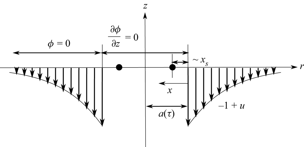
Appendix B. further considerations on the scaling of the thin film thickness
Figure 7 explores the case in which the transition between the capillary and inertial regimes took place for  $We St^{-1/6}=C$ with
  $C>1$ a constant such that all the experimental data in de Ruiter et al. (Reference de Ruiter, Oh, van den Ende and Mugele2012) laid in the capillary regime. If that was the case, the data corresponding to both ethanol and water reported by de Ruiter et al. (Reference de Ruiter, Oh, van den Ende and Mugele2012) should be scaled introducing a common prefactor in (2.20). The better agreement between predictions and experiments depicted in figure 2, where no prefactors are introduced, suggest to establish the transition between the inertial and the capillary scalings at
  $We St^{-1/6}\simeq 1$.
Comparison of the predictions given in (2.15) and (2.20) with the experimental data in figure 3(a) in de Ruiter et al. (Reference de Ruiter, Oh, van den Ende and Mugele2012), being the only difference with the results shown in figure 2 that (2.20) for  $h_m/R$ corresponding to the capillary scaling is multiplied by a constant factor
  $K=0.65$. If all the experiments in the figure laid in the capillary regime, all the data corresponding to both water and ethanol could be approximated introducing a prefactor in (2.20). The results in this figure and in figure 2 suggest to establish the transition between the inertial and the capillary scalings at
  $We St^{-1/6}\simeq 1$, this condition being indicated in the figure with the two vertical lines.
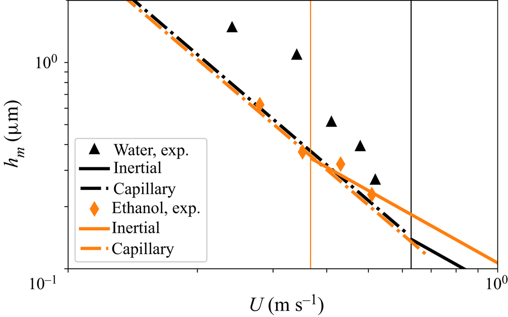
Appendix C. Influence of heat flux across the thermal boundary layer
The net heat flux to the evaporating interface needs to take into account the heat flux transferred into the liquid through the thermal boundary layer. We make use of the result by Roisman (Reference Roisman2009), Eggers et al. (Reference Eggers, Fontelos, Josserand and Zaleski2010), who analysed the spatio-temporal structure of the momentum boundary layer developing at the wall after a drop hits a surface for instants of time  $\tau \ll 1$, finding that the thickness of the momentum boundary layer scales as
 \begin{equation} \lambda_u\propto\sqrt{\nu_l (R/U)\tau_m}\end{equation}
for  $r\lesssim R\sqrt {3\tau _m}$. In the case of a heated wall, the analogy between the momentum and thermal boundary layer equations and of their corresponding boundary conditions, indicates that the thermal boundary layer thickness scales as (Schlichting & Gersten Reference Schlichting and Gersten2000)
 \begin{equation} \lambda_\theta\propto Pr^{{-}1/2} \lambda_u=K R Pr^{{-}1/2} Re^{{-}1/2} \tau^{1/2}_m ,\end{equation}
where use of (C1) has been made and  $K$ is an order unity dimensionless proportionality constant. Note that the
  $Pr^{-1/2}$ scaling in (C2) results from the fact that the shear stresses at the dimple gas–liquid interface are small and, hence, the liquid velocity profile inside the thermal boundary layer can be considered as uniform. Consequently, the heat power per unit area transferred by conduction into the liquid along the region which is separated from the wall a distance
  $h_m$ can be estimated, using a one-dimensional approach, as
 \begin{equation} k_l\frac{T_b-T_a}{\lambda_\theta}, \end{equation}
with  $\lambda _\theta$ given in (C2) and where we have taken into account that the initial liquid temperature is the same as that of the surrounding gaseous atmosphere,
  $T_a$. Therefore, the net heat power per unit area which is transferred to the evaporating interface is given by (see (2.21))
 \begin{equation} k_v\frac{{\rm \Delta} T}{h_m}\left(1-\frac{k_l Pr^{1/2}}{k_v K\sqrt{C_\tau}}\sqrt{\frac{\eta_a}{\eta_l}}St^{5/6}\frac{T_b-T_a}{{\rm \Delta} T}\frac{h_m}{R}\right) .\end{equation}
The relative importance of heat conduction across the boundary layer in (C4) can be quantified inserting the value of  $h_{m}/R$ of (2.27) into (C4). But, note that
  $\beta ^{*}$, defined in (2.26a,b), is such that
  $\beta ^{*}\gg 1$ and, therefore, the following simplified solution of (2.25) can be obtained:
 \begin{equation} \frac{h_m}{R}\sim C_\tau \left(\frac{\rho_l}{\rho_v}\right)^{1/4}\left(\frac{\eta_v}{\eta_a}\right)^{1/2} St^{{-}7/6} \beta^{1/4}. \end{equation}
Consequently,
 \begin{equation} \frac{h_m}{h_{a,m}} \sim \left(\frac{\rho_l}{\rho_v}\right)^{1/4}\left(\frac{\eta_v}{\eta_a}\right)^{1/2} \beta^{1/4} St^{{-}1/6} .\end{equation}
Therefore, the role of the heat flux across the liquid thermal boundary layer can be quantified through the value of the parameter
 \begin{equation} \sqrt{\frac{k_l C_{p,l}}{k_v C_{p,v}}}\left(\frac{\rho_l}{\rho_v}\right)^{1/4}\beta_a \beta^{{-}3/4} St^{{-}1/3} , \end{equation}
where we have substituted (C5) into (C4),  $C_{p,l}$ is the liquid heat capacity at constant pressure,
  $\beta _a$ is defined in (2.3a,b) and where we have also taken into account that the vapour Prandtl number is always close to unity. The value of the parameter (C7) is small for the range of values of
  $\beta$ and
  $St$ reported by Chantelot & Lohse (Reference Chantelot and Lohse2021), which supports the approximation followed in the main text. However, (C7) also reveals that the relative importance of the heat flux into the liquid increases as either the impact velocity – within the range
  $We St^{-1/6}\gtrsim 1$ – or the value of the superheat, decreases. Note also that if the liquid at the bottom of the impacting drop is preheated by the surrounding atmosphere before reaching the substrate up to values of the temperature close to
  $T_b$ then
  $\beta _a\simeq 0$ and, consequently, the heat flux from the superheated wall is totally directed to produce vapour, which would support even further the approximation followed in the main text.
Appendix D. Fluid properties
The values of the physical properties for the case of superheated substrates are not kept constant, but are considered to depend on the averaged temperature  $T=(T_s+T_b)/2$, with
  $T$ in celsius (Sobac et al. Reference Sobac, Rednikov, Dorbolo and Colinet2014). The vapour density at the neck region is calculated using the ideal gas law and assuming that the pressure is the averaged one along the region of length
  $h_{a,m}$ located downstream of the stagnation point,
 \begin{equation} \rho_v=\rho_{v 0} \left(\frac{273+78}{273+T}\right)\times\varPi_r\quad\text{with } \varPi_r=\left(1+\rho_l U^{2} \frac{9 {{St}}^{2/3}}{32 C_\tau\times 10^{5}}\right) .\end{equation}
 The pressure  $P$ at the neck region changes as a consequence of the different impact velocities,
  $P\simeq 10^{5}\times \varPi _r$ Pa, with
  $\varPi _r$ defined in (D1). These changes modify the value of the boiling temperature through the Antoine equation and, hence, also the value of the latent heat of vaporization with respect to the values given in table 1. However, these differences with respect to the values provided in the table are small and are not considered for the range of experimental data reported in Chantelot & Lohse (Reference Chantelot and Lohse2021).
Physical properties of air and liquid and vapour ethanol used in this study.

Also, note that  $\beta$, defined in (2.3a,b), is calculated here as
 \begin{equation} \beta=\frac{k_v {\rm \Delta} T}{\eta_v \mathcal{L}}=Pr^{{-}1}_v C_{p,v} \frac{{\rm \Delta} T}{\mathcal{L}}, \end{equation}
namely, as a function of the vapour Prandtl number, which is very close to 1 and hardly varies with temperature, see table 1, and of the heat capacity of the vapour at constant pressure,  $C_{p,v}$ which is approximated using the tabulated data for ethanol (ToolBox, Engineering 2018b),
 \begin{equation} C_{p ,v}=\left(1830+250\frac{(T-78)}{100}\right)\quad \text{J\ (kg K)}^{{-}1}. \end{equation}
Since the values of the vapour and air viscosities notably deviate from those calculated using the gas kinetic theory, these are approximated using the following fittings to the tabulated data (ToolBox, Engineering 2003, 2018a):
 \begin{gather} \eta_v=\eta_{v 0}\left[\frac{273+T}{273+78}\right]^{1.2}, \end{gather}
 \begin{gather}\eta_a=\eta_{a 0}\left[\frac{273+T}{300}\right]^{0.7}, \end{gather}
with the values of  $\eta _{v 0}$ and
  $\eta _{a 0}$ given in table 1.


 Open access