


1. Introduction
As a passive flow control technique, the compliant wall has gained significant attention for its simplicity, low cost and no need for external power. The compliant wall modulates flow structures through dynamic motion and deformation in response to flow-induced pressure variations. As early as the 1960s, inspired by the exceptional swimming capabilities of dolphins, Kramer (Reference Kramer1961) utilized a rubber sheet with tiny rubber stubs to imitate the soft skin of dolphins and discovered drag reduction. Subsequent research pointed out significant experimental errors in these earlier experiments (Bushnell, Hefner & Ash Reference Bushnell, Hefner and Ash1977). Nevertheless, stability theory has demonstrated that compliant walls can postpone flow transition through the interaction between the Tollmien–Schlichting wave and wall wavy movement (Benjamin Reference Benjamin1960; Carpenter & Garrad Reference Carpenter and Garrad1985, Reference Carpenter and Garrad1986). While there is consensus regarding the efficacy of compliant walls in transitional flows, their role in reducing skin-friction drag within fully developed turbulence remains a subject of ongoing debate (Bushnell et al. Reference Bushnell, Hefner and Ash1977; Riley, Gad-el Hak & Metcalfe Reference Riley, Gad-el-Hak and Metcalfe1988; Gad-el-Hak Reference Gad-el-Hak2002).
For fully developed turbulent flows, early experimental series have also shown that compliant walls can reduce Reynolds stress and skin friction (Lee, Fisher & Schwarz Reference Lee, Fisher and Schwarz1993; Choi et al. Reference Choi, Yang, Clayton, Glover, Atlar, Semenov and Kulik1997). However, most results of direct numerical simulation (DNS) have found that a compliant wall either shows little effect or even increases resistance. For example, Xu, Rempfer & Lumley (Reference Xu, Rempfer and Lumley2003) employed a spring-supported isotropic model and observed no significant differences in turbulence statistical quantities or skin friction coefficients compared with rigid walls. Their linear stability analysis further revealed that excessive wall compliance introduces unstable eigenmodes, potentially generating static-divergence waves that increase skin friction. Kim & Choi (Reference Kim and Choi2014) found that stiffer compliant walls have little impact on surface friction drag and the flow structures, while soft compliant walls increase total drag because wall deformations propagate downstream as large-amplitude quasi-two-dimensional waves. These waves exhibit positive pressure on the upslope and negative pressure on the downslope regions, resulting in a significant drag increase. Xia, Huang & Xu (Reference Xia, Huang and Xu2017) used monoharmonic analysis for selection of compliant wall parameters, yet all tested cases resulted in increased skin-friction drag due to enhanced Reynolds shear stress and mean convection terms, based on the drag coefficient decomposition developed by Fukagata, Iwamoto & Kasagi (Reference Fukagata, Iwamoto and Kasagi2002). Moreover, Fukagata et al. (Reference Fukagata, Kern, Chatelain and Kasagi2008) employed an anisotropic spring model that allows tangential deformation, but even the optimized drag-reducing compliant wall still increases friction when the computational domain was doubled in the streamwise direction. Subsequent DNS results have also failed to identify an anisotropic compliant wall that can reduce drag (Xia, Huang & Xu Reference Xia, Huang and Xu2019).
The convective velocity of wall-pressure fluctuations and wall displacement plays a pivotal role in compliant wall–turbulence interactions. As demonstrated by Kim & Choi (Reference Kim and Choi2014), compliant walls with low stiffness develop large-amplitude quasi-two-dimensional waves propagating downstream at reduced convective velocities ( $c_\eta \lt 0.4U_c$
), amplifying drag through resonant pressure fluctuations and enhanced vortical activity. Over anisotropic compliant walls, Fukagata et al. (Reference Fukagata, Kern, Chatelain and Kasagi2008) also found the downstream-travelling waves on the compliant wall associated with a convective velocity of
$c_\eta \lt 0.4U_c$
), amplifying drag through resonant pressure fluctuations and enhanced vortical activity. Over anisotropic compliant walls, Fukagata et al. (Reference Fukagata, Kern, Chatelain and Kasagi2008) also found the downstream-travelling waves on the compliant wall associated with a convective velocity of $c_\eta \approx 0.35U_c$
(
$c_\eta \approx 0.35U_c$
( $c_\eta \approx 6$
) and wavelengths matching the computational domain scale. Experiments of turbulent flow over compliant walls observed the deformation waves travelling at
$c_\eta \approx 6$
) and wavelengths matching the computational domain scale. Experiments of turbulent flow over compliant walls observed the deformation waves travelling at $0.53$
times the free stream velocity at Reynolds numbers
$0.53$
times the free stream velocity at Reynolds numbers $ \textit{Re}_\tau =$
3300, 6700 and 8900 (Lu et al. Reference Lu, Xiang, Zaki and Katz2024), and the flow–deformation correlation decreases with increasing Reynolds number (Lu et al. Reference Lu, Xiang, Zaki and Katz2025). Other studies have reported the convective velocity of wall displacement varying between approximately
$ \textit{Re}_\tau =$
3300, 6700 and 8900 (Lu et al. Reference Lu, Xiang, Zaki and Katz2024), and the flow–deformation correlation decreases with increasing Reynolds number (Lu et al. Reference Lu, Xiang, Zaki and Katz2025). Other studies have reported the convective velocity of wall displacement varying between approximately $0.3$
and
$0.3$
and $0.8$
times free stream velocity, depending on wall properties, e.g.
$0.8$
times free stream velocity, depending on wall properties, e.g. $0.28-0.78$
in Kim & Choi (Reference Kim and Choi2014) with softer walls exhibiting lower values,
$0.28-0.78$
in Kim & Choi (Reference Kim and Choi2014) with softer walls exhibiting lower values, $0.65$
in Esteghamatian, Katz & Zaki (Reference Esteghamatian, Katz and Zaki2022),
$0.65$
in Esteghamatian, Katz & Zaki (Reference Esteghamatian, Katz and Zaki2022), $0.66$
in Wang, Koley & Katz (Reference Wang, Koley and Katz2020),
$0.66$
in Wang, Koley & Katz (Reference Wang, Koley and Katz2020), $0.72$
in Zhang et al. (Reference Zhang, Wang, Blake and Katz2017) and
$0.72$
in Zhang et al. (Reference Zhang, Wang, Blake and Katz2017) and $0.70-0.80$
in Greidanus et al. (Reference Greidanus, Delfos, Picken and Westerweel2022).
$0.70-0.80$
in Greidanus et al. (Reference Greidanus, Delfos, Picken and Westerweel2022).
The input–output analysis (IOA), which is closely related to resolvent analysis, was originally employed in wall-bounded shear flow analysis based on a linearized Navier–Stokes equations (NSEs) system driven by stochastic input forcing (Farrell & Ioannou Reference Farrell and Ioannou1993). The IOA technique can characterize the energy amplification to study transition to turbulence (Farrell & Ioannou Reference Farrell and Ioannou1993; Bamieh & Dahleh Reference Bamieh and Dahleh2001; Jovanović & Bamieh Reference Jovanović and Bamieh2005) and can also be used to identify coherent structures in high-Reynolds-number wall turbulence (McKeon & Sharma Reference McKeon and Sharma2010; McKeon Reference McKeon2017), see review papers (Schmid Reference Schmid2007; Jovanović Reference Jovanović2021). The resolvent analysis, as a reduced-order modelling framework, has been used to optimize the compliant wall parameters and predict flow structures under the passive control of the compliant walls (Luhar et al. Reference Luhar, Sharma and McKeon2015, Reference Luhar, Sharma and McKeon2016; Jafari, McKeon & Arjomandi Reference Jafari, McKeon and Arjomandi2023). Luhar, Sharma & McKeon (Reference Luhar, Sharma and McKeon2015) used the resolvent analysis to select optimal walls under two energetic flow structures in wall turbulence. The results reveal that walls with negative damping coefficients exhibit enhanced suppression of near-wall cycles, while positive damping configurations are effective for suppressing very large-scale motions (VLSMs). However, the optimized walls did not achieve consistent turbulence suppression across the entire spectral range (Luhar et al. Reference Luhar, Sharma and McKeon2015). Luhar, Sharma & McKeon (Reference Luhar, Sharma and McKeon2016) further applied this resolvent analysis framework to examine the influence of compliant wall parameters with varying mass ratio, tension, stiffness and anisotropy. The computational results show that the influence of these wall parameters is concentrated around the resonance frequency conditions, and compliant walls tend to amplify flow structures that are slower-moving and uniform in the spanwise direction (i.e. two-dimensional structures). To overcome the limitation that the original compliant wall impedance model only reflects normal pressure and normal velocity interaction (Luhar et al. Reference Luhar, Sharma and McKeon2015), Jafari et al. (Reference Jafari, McKeon and Arjomandi2023) expanded the boundary conditions of the IOA method by incorporating tangential stress-velocity coupling mechanisms. The generalized impedance matrix introduced in this study (Jafari et al. Reference Jafari, McKeon and Arjomandi2023) includes transpiration and slip at the wall under both pressure and shear responses. The input–output or resolvent analysis can also be applied in other flow control strategies, such as streamwise travelling waves, transverse wall oscillation, opposition control and suboptimal control (Moarref & Jovanović Reference Moarref and Jovanović2010; Moarref & Jovanović Reference Moarref and Jovanović2012; Luhar et al. Reference Luhar, Sharma and McKeon2014b ; Nakashima, Fukagata & Luhar Reference Nakashima, Fukagata and Luhar2017).
The structured input-output analysis (SIOA) method extends the IOA framework by incorporating a structured uncertainty feedback loop to capture nonlinear interactions, with a computational cost similar to traditional IOA (Liu & Gayme Reference Liu and Gayme2021). The SIOA method has been shown to identify oblique waves (Liu & Gayme Reference Liu and Gayme2021; Liu et al. Reference Liu, Shuai, Rath and Gayme2023; Rath, Liu & Gayme Reference Rath, Liu and Gayme2024) and oblique turbulent bands (Liu Reference Liu2021; Liu, Caulfield & Gayme Reference Liu, Caulfield and Gayme2022; Shuai, Liu & Gayme Reference Shuai, Liu and Gayme2023) in transitional wall-bounded shear flows consistent with DNS and experimental observations. These findings demonstrate that the SIOA framework can effectively capture nonlinear behaviours. Moreover, SIOA has also been employed to identify dominant flow structures in turbulent flows over riblets (Mushtaq, Luhar & Hemati Reference Mushtaq, Luhar and Hemati2023b ) and compressible flows (Bhattacharjee et al. Reference Bhattacharjee, Mushtaq, Seiler and Hemati2024).
To model the effect of small-scale turbulence on larger-scale diffusion, Reynolds & Tiederman (Reference Reynolds and Tiederman1967) proposed an eddy viscosity enhancement to linearized NSE. The eddy-viscosity-enhanced IOA model (IOA-e) has been found to accurately predict the spanwise spacing of near-wall streaks (del Álamo & Jiménez Reference del Álamo and Jiménez2006; Cossu, Pujals & Depardon Reference Cossu, Pujals and Depardon2009; Pujals et al. Reference Pujals, García-Villalba, Cossu and Depardon2009; Hwang & Cossu Reference Hwang and Cossu2010a , Reference Hwang and Cossub ; Symon et al. Reference Symon, Madhusudanan, Illingworth and Marusic2023) and estimate large-scale structures (Illingworth, Monty & Marusic Reference Illingworth, Monty and Marusic2018; Morra et al. Reference Morra, Semeraro, Henningson and Cossu2019; Madhusudanan, Illingworth & Marusic Reference Madhusudanan, Illingworth and Marusic2019). The IOA-e method can also improve the prediction in compressible turbulent boundary layers (Fan et al. Reference Fan, Kozul, Li and Sandberg2024), and the eddy viscosity profile can be optimized by minimizing the spatial correlations of the stochastic forcing (Ying et al. Reference Ying, Chen, Li and Fu2024). However, the eddy viscosity enhancement of the SIOA framework remains unexplored.
This study pioneers the investigation of SIOA-e and examines its ability to identify coherent structures in high-Reynolds-number turbulent channel flows over both rigid and compliant walls. We employ the SIOA-e method to identify near-wall cycles and VLSMs over rigid walls. Furthermore, we employ SIOA-e to optimize compliant-wall parameters for suppressing energetically dominant flow structures (near-wall cycle or VLSMs) and evaluate the effect of optimized compliant wall parameters on flow structures over a wide range of spatiotemporal scales. We further analyse convective velocities of velocity and pressure fluctuations in both rigid-wall and compliant-wall turbulent flows using the IOA framework (Liu & Gayme Reference Liu and Gayme2020), where the pressure convective velocities in rigid-wall turbulent channel flows are compared with DNS studies (Kim & Hussain Reference Kim and Hussain1993; Mehrez, Yamamoto & Tsuji Reference Mehrez, Yamamoto and Tsuji2023). Moreover, we also compute convective velocities of wall displacement in compliant-wall turbulence, which agree well with the convective velocity of wall displacement measured in laboratory experiments (Lu et al. Reference Lu, Xiang, Zaki and Katz2024). Finally, we investigate the scale dependence of convective velocities, identifying spatiotemporal flow scales strongly influenced by the compliant walls.
The rest of the paper is organized as follows. Section 2 establishes the problem formulation with boundary conditions for both rigid and compliant walls, followed by a brief overview of the IOA, SIOA, IOA-e and SIOA-e models. The input–output amplification over rigid walls characteristics by SIOA-e and the comparison with other three models, are shown in § 3. We then validate the compliant-wall modelling with Kim & Choi (Reference Kim and Choi2014) and Xia et al. (Reference Xia, Huang and Xu2017) in § 4, and optimize the compliant wall parameters using models with eddy-viscosity by minimizing the structured and unstructured singular values associated with near-wall cycle and VLSMs at Reynolds number $ \textit{Re}_\tau = 2000$
. Section 5 computes convective velocities for velocity components, pressure fluctuations and wall displacement for rigid and compliant walls, which are compared with rigid-wall DNS studies (Kim & Hussain Reference Kim and Hussain1993; Mehrez et al. Reference Mehrez, Yamamoto and Tsuji2023) and recent experimental measurements of turbulent flow over compliant walls (Lu et al. Reference Lu, Xiang, Zaki and Katz2024). Finally, conclusions and potential future work are discussed in § 6.
$ \textit{Re}_\tau = 2000$
. Section 5 computes convective velocities for velocity components, pressure fluctuations and wall displacement for rigid and compliant walls, which are compared with rigid-wall DNS studies (Kim & Hussain Reference Kim and Hussain1993; Mehrez et al. Reference Mehrez, Yamamoto and Tsuji2023) and recent experimental measurements of turbulent flow over compliant walls (Lu et al. Reference Lu, Xiang, Zaki and Katz2024). Finally, conclusions and potential future work are discussed in § 6.
2. Methodology
In this section, we start by describing the problem set-up and boundary conditions for rigid and compliant walls. We then introduce the IOA, SIOA and the incorporation of eddy viscosity in both models (IOA-e and SIOA-e).
2.1. Problem set-up and boundary conditions
This paper considers fully developed turbulent channel flow over the compliant wall and employs $x$
,
$x$
, $y$
and
$y$
and $z$
to, respectively, denote the streamwise, wall-normal and spanwise directions, as seen in figure 1(a). The NSEs for velocity fluctuations in turbulent channel flows are given as follows:
$z$
to, respectively, denote the streamwise, wall-normal and spanwise directions, as seen in figure 1(a). The NSEs for velocity fluctuations in turbulent channel flows are given as follows:
 \begin{align} \frac {\partial \boldsymbol{u}}{\partial t} + (\boldsymbol{u} \boldsymbol{\cdot }\boldsymbol{\nabla })\boldsymbol{U} + (\boldsymbol{U} \boldsymbol{\cdot }\boldsymbol{\nabla })\boldsymbol{u} + \boldsymbol{\nabla }p - \frac {1}{Re_\tau }{\nabla} ^2 \boldsymbol{u} &= -(\boldsymbol{u} \boldsymbol{\cdot }\boldsymbol{\nabla })\boldsymbol{u} + \langle (\boldsymbol{u} \boldsymbol{\cdot }\boldsymbol{\nabla })\boldsymbol{u}\rangle , \\[-12pt] \nonumber \end{align}
 \begin{align} \boldsymbol{\nabla }\boldsymbol{\cdot }\boldsymbol{u} &= 0. \\[10pt] \nonumber \end{align}
The velocities in the three coordinate directions are turbulent mean flow $\boldsymbol{U}=[U(y),0,0]^\top$
with fluctuations
$\boldsymbol{U}=[U(y),0,0]^\top$
with fluctuations $\boldsymbol{u}=[u,v,w]^\top$
. The pressure fluctuation is
$\boldsymbol{u}=[u,v,w]^\top$
. The pressure fluctuation is $p$
. The angled brackets
$p$
. The angled brackets $\langle \boldsymbol{\cdot }\rangle$
mean ensemble average. The friction Reynolds number is defined as
$\langle \boldsymbol{\cdot }\rangle$
mean ensemble average. The friction Reynolds number is defined as $ \textit{Re}_\tau = u_\tau h / \nu$
, where
$ \textit{Re}_\tau = u_\tau h / \nu$
, where $h$
is the channel half-height,
$h$
is the channel half-height, $u_\tau$
is the friction velocity and
$u_\tau$
is the friction velocity and $\nu$
denotes the kinematic viscosity. Here, velocity is normalized by
$\nu$
denotes the kinematic viscosity. Here, velocity is normalized by $u_\tau$
, length is normalized by
$u_\tau$
, length is normalized by $h$
and time is normalized by
$h$
and time is normalized by $h/u_\tau$
. The superscript
$h/u_\tau$
. The superscript $^+$
is used to denote the length normalized by the viscous length scale
$^+$
is used to denote the length normalized by the viscous length scale $\delta _\nu =\nu /u_\tau$
to distinguish from the length normalized by
$\delta _\nu =\nu /u_\tau$
to distinguish from the length normalized by $h$
. Note that all velocity variables are normalized by
$h$
. Note that all velocity variables are normalized by $u_\tau$
here, so the superscript
$u_\tau$
here, so the superscript $^+$
is therefore omitted for velocity variables to simplify notation.
$^+$
is therefore omitted for velocity variables to simplify notation.
Schematic diagram of (a) the turbulent channel flow between two compliant walls and (b) compliant wall model with spring and damping.

We then exploit spatial shift-invariance in the streamwise and spanwise directions and assume the shift-invariance in time, which leads to the triple Fourier transform of velocity and pressure,
 \begin{align} \begin{bmatrix} \hat { \boldsymbol{ u } } \left ( y ; k _ { x } , k _ { z } , \omega \right ) \\[3pt] \hat { p } \left ( y ; k _ { x } , k _ { z } , \omega \right ) \end{bmatrix} = \iiint _ {-\infty }^{\infty } \begin{bmatrix} \boldsymbol{u}(x,y,z,t) \\[3pt] p(x,y,z,t) \end{bmatrix} e ^ {- \mathrm{i} \left (k_{x}x + k_{z}z- \omega t \right )} \mathrm{d}x\, \mathrm{d}z\, \mathrm{d}t, \end{align}
where $\rm {i}=\sqrt {-1}$
is the imaginary unit and
$\rm {i}=\sqrt {-1}$
is the imaginary unit and $k_x = 2 \pi / \lambda _x$
and
$k_x = 2 \pi / \lambda _x$
and $k_z = 2\pi / \lambda _z$
are dimensionless streamwise and spanwise wavenumbers, respectively. Here
$k_z = 2\pi / \lambda _z$
are dimensionless streamwise and spanwise wavenumbers, respectively. Here $\omega$
is the temporal frequency and
$\omega$
is the temporal frequency and $\omega =ck_x$
, where
$\omega =ck_x$
, where $c$
is the phase speed normalized by friction velocity.
$c$
is the phase speed normalized by friction velocity.
For turbulence between rigid walls, we impose no-slip and no-penetration boundary conditions at the wall; i.e. $\hat {\boldsymbol{u}}(y=\pm 1) = 0$
. In the case of compliant walls, we follow the same modelling procedure as the previous work (Luhar et al. Reference Luhar, Sharma and McKeon2015) for a direct comparison, where the wall displacement is assumed to be small. Here, we need both kinematic boundary conditions and dynamic boundary conditions. To simplify the problem, this paper considers the wall that can only move upward in the wall-normal
$\hat {\boldsymbol{u}}(y=\pm 1) = 0$
. In the case of compliant walls, we follow the same modelling procedure as the previous work (Luhar et al. Reference Luhar, Sharma and McKeon2015) for a direct comparison, where the wall displacement is assumed to be small. Here, we need both kinematic boundary conditions and dynamic boundary conditions. To simplify the problem, this paper considers the wall that can only move upward in the wall-normal $y$
direction without movement in
$y$
direction without movement in $x$
and
$x$
and $z$
directions. The wall-normal displacement of the compliant wall is
$z$
directions. The wall-normal displacement of the compliant wall is $\eta (x,z,t)$
, where
$\eta (x,z,t)$
, where $x$
and
$x$
and $z$
are independent of time
$z$
are independent of time $t$
. The no-slip and no-penetration boundary conditions at the compliant wall surface indicate the velocity at the wall is the same as the velocity of the wall movement, i.e.
$t$
. The no-slip and no-penetration boundary conditions at the compliant wall surface indicate the velocity at the wall is the same as the velocity of the wall movement, i.e. $u(\eta )=0$
,
$u(\eta )=0$
, $v(\eta )=\partial _t \eta$
and
$v(\eta )=\partial _t \eta$
and $w(\eta )=0$
. After Taylor expansion, the small quantities of higher orders are omitted, and only the linear terms of the first order are retained. The linearization is based on the small-displacement approximation, which is reliably valid for wall deformation amplitudes
$w(\eta )=0$
. After Taylor expansion, the small quantities of higher orders are omitted, and only the linear terms of the first order are retained. The linearization is based on the small-displacement approximation, which is reliably valid for wall deformation amplitudes $\eta ^{+} \lesssim 5$
within the viscous sublayer (normalized by the viscous length scale
$\eta ^{+} \lesssim 5$
within the viscous sublayer (normalized by the viscous length scale $\delta _\nu$
), as supported by early work (Semenov Reference Semenov1991) and modern DNS studies (Xu et al. Reference Xu, Rempfer and Lumley2003; Xia et al. Reference Xia, Huang and Xu2017). The kinematic boundary conditions after the linearization and Fourier transformation are reduced to (here take the bottom wall as an example)
$\delta _\nu$
), as supported by early work (Semenov Reference Semenov1991) and modern DNS studies (Xu et al. Reference Xu, Rempfer and Lumley2003; Xia et al. Reference Xia, Huang and Xu2017). The kinematic boundary conditions after the linearization and Fourier transformation are reduced to (here take the bottom wall as an example)
 \begin{align} \hat {u}({y=-1 +} \eta ) &\approx \hat {u}(y=- 1) + \hat {\eta } \left . \frac {\mathrm{d} U}{\mathrm{d} y} \right |_{y=- 1} = 0, \\[-12pt] \nonumber \end{align}
 \begin{align} \hat {v}({y=-1 +} \eta ) &\approx \hat {v}(y=- 1) = -\mathrm{i} \omega \hat {\eta }, \\[-10pt] \nonumber \end{align}
 \begin{align} \hat {w}({y=-1 +} \eta ) &\approx \hat {w}(y=- 1) = 0. \\[10pt] \nonumber \end{align}
The kinematic boundary condition (2.3a
) imposes the no-slip condition at the moving wall $y = -1+\eta$
. As a result, the streamwise velocity fluctuation
$y = -1+\eta$
. As a result, the streamwise velocity fluctuation $\hat {u}(y=- 1)$
needs to offset the effects of the mean flow induced by the wall displacement associated with the term
$\hat {u}(y=- 1)$
needs to offset the effects of the mean flow induced by the wall displacement associated with the term $\hat {\eta } \left . ({\mathrm{d} U}/{\mathrm{d} y} )\right |_{y=- 1}$
, which can lead to non-zero value of
$\hat {\eta } \left . ({\mathrm{d} U}/{\mathrm{d} y} )\right |_{y=- 1}$
, which can lead to non-zero value of $\hat {u}(y=- 1)\neq 0$
. Accordingly, the kinematic boundary condition is applied at
$\hat {u}(y=- 1)\neq 0$
. Accordingly, the kinematic boundary condition is applied at $y=1-\eta$
at the top wall.
$y=1-\eta$
at the top wall.
The dynamic boundary condition then relates the wall displacement $\eta$
to the pressure fluctuations
$\eta$
to the pressure fluctuations $p$
in turbulent flows over compliant walls. Here, the compliant wall is modelled as a membrane supported by a spring and a damper, as shown in figure 1(b). From the spring-damper model, the dimensionless momentum equation at the wall can be obtained as
$p$
in turbulent flows over compliant walls. Here, the compliant wall is modelled as a membrane supported by a spring and a damper, as shown in figure 1(b). From the spring-damper model, the dimensionless momentum equation at the wall can be obtained as
 \begin{align} C_m\frac { { d } ^ { 2 } \eta } { \mathrm{ d } t ^ { 2 } } + C_d \frac { \mathrm{ d } \eta } { \mathrm{ \, d } t } + C_k \eta = - p(y=-1). \end{align}
Here, the dimensionless parameters of mass factor $C_{m}$
, damping coefficient
$C_{m}$
, damping coefficient $C_{d}$
and stiffness coefficient
$C_{d}$
and stiffness coefficient $C_{k}$
are
$C_{k}$
are
 \begin{align} C _ { m } = \frac { \rho _ { w } } { \rho h } ,\quad C _ { d } = \frac { d _ { w } } { \rho u _ { \tau } } \quad \text{and} \quad C _ { k } = \frac { k _ { w } h } { \rho u _ { \tau } ^ { 2 } }, \end{align}
where $\rho _w$
denotes the compliant wall’s mass per unit area,
$\rho _w$
denotes the compliant wall’s mass per unit area, $\rho$
is the fluid density and
$\rho$
is the fluid density and $k_{w}$
and
$k_{w}$
and $d_{w}$
represent the stiffness and damping coefficients per unit area, respectively. After performing the Fourier transform, we get the dimensionless formula
$d_{w}$
represent the stiffness and damping coefficients per unit area, respectively. After performing the Fourier transform, we get the dimensionless formula
 \begin{align} \big ( - C _ { m } \omega ^2- \textrm {i} \omega C _ { d } + C _ { k } \big ) \hat { \eta } = - \hat { p }(y=-1). \end{align}
The resonance frequency $\omega _r$
of the damped vibration of the compliant wall is then found to be
$\omega _r$
of the damped vibration of the compliant wall is then found to be
 \begin{align} \omega _r =\omega _n \sqrt {1-2\zeta ^2}. \end{align}
Here, $\omega _n = \sqrt {{C_k}/{C_m}}$
is the undamped natural frequency of the wall, and
$\omega _n = \sqrt {{C_k}/{C_m}}$
is the undamped natural frequency of the wall, and $\zeta ={C_d}/{2\sqrt {C_k C_m}}$
is the damping factor. Parameters characterizing the wall properties can also be expressed in terms of wall mechanical admittance
$\zeta ={C_d}/{2\sqrt {C_k C_m}}$
is the damping factor. Parameters characterizing the wall properties can also be expressed in terms of wall mechanical admittance $Y$
, which has been used previously by Landahl (Reference Landahl1962), Sen & Arora (Reference Sen and Arora1988) and Luhar et al. (Reference Luhar, Sharma and McKeon2015). The wall mechanical admittance reflects the normal motion velocity of the wall at unit pressure, and its relation to the parameters
$Y$
, which has been used previously by Landahl (Reference Landahl1962), Sen & Arora (Reference Sen and Arora1988) and Luhar et al. (Reference Luhar, Sharma and McKeon2015). The wall mechanical admittance reflects the normal motion velocity of the wall at unit pressure, and its relation to the parameters $C_{m}$
,
$C_{m}$
, $C_{d}$
and
$C_{d}$
and $C_{k}$
can be obtained from (2.3) and (2.6):
$C_{k}$
can be obtained from (2.3) and (2.6):
 \begin{align} \begin{aligned} Y&=\frac {\hat {v}(-1)}{\hat {p}(-1)} \\&=-\frac {\omega ^2 C_d}{(C_k-\omega ^2 C_m)^2+\omega ^2 C_d^2}+\textrm {i}\frac {\omega \big(C_k-\omega ^2 C_m \big)}{\big(C_k-\omega ^2 C_m \big)^2+\omega ^2 C_d^2} \\&=:{\rm {Re}}(Y)+\text{i}\,{\rm {Im}}(Y). \end{aligned} \end{align}
Here, Re and Im represent the real and imaginary parts, respectively. Since the differing symmetry of the pressure and wall-normal velocity to the centreline, the sign of mechanical admittance on the upper wall is opposite to that on the bottom, i.e. $Y=-{\hat {v}(1)}/{\hat {p}(1)}$
(Luhar et al. Reference Luhar, Sharma and McKeon2015). Note that the formulation of IOA type analysis does not include the wall displacement
$Y=-{\hat {v}(1)}/{\hat {p}(1)}$
(Luhar et al. Reference Luhar, Sharma and McKeon2015). Note that the formulation of IOA type analysis does not include the wall displacement $\eta$
as a state variable, so the wall displacement term in the boundary condition needs to be replaced by the pressure. By substituting the dynamic boundary conditions (2.8) into the kinematic boundary conditions (2.3), the boundary conditions about velocity and pressure fields can be obtained:
$\eta$
as a state variable, so the wall displacement term in the boundary condition needs to be replaced by the pressure. By substituting the dynamic boundary conditions (2.8) into the kinematic boundary conditions (2.3), the boundary conditions about velocity and pressure fields can be obtained:
 \begin{align} \begin{aligned} - \textrm {i} \omega \hat { u } ( y = \pm 1 ) \mp Y \left . \frac { \mathrm{ d } U } { \mathrm{ d } y } \right | _ { y=\pm 1 } \hat { p } ( y=\pm 1 ) &= 0, \\[3pt]\hat { v } (y= \pm 1 ) \pm Y \hat { p } ( y = \pm 1 ) &= 0, \\[3pt]\hat { w } ( y=\pm 1 ) &= 0. \\ \end{aligned} \end{align}
Here, the boundary condition at $y=1$
is obtained in the same spirit as that at
$y=1$
is obtained in the same spirit as that at $y=-1$
considering the symmetry with respect to the channel centreline.
$y=-1$
considering the symmetry with respect to the channel centreline.
2.2. Input–output analysis formulation
In the IOA model, the NSEs are linearized as a linear operator in spectral space. All nonlinear terms in the NSEs are treated as input forcing to this linearized system, generating velocity and pressure responses. Specifically, two nonlinear terms on the right-hand side of (2.1a ) are treated as input forcing in IOA, denoted as
 \begin{align} -(\boldsymbol{u}\boldsymbol{\cdot }\boldsymbol{\nabla })\boldsymbol{u} + \langle (\boldsymbol{u} \boldsymbol{\cdot }\boldsymbol{\nabla })\boldsymbol{u}\rangle =\boldsymbol{f}. \end{align}
After conducting the Fourier transform of NSEs, we have the resulting system as
 \begin{align} -{\rm {i}} \omega \begin{bmatrix} \mathcal{I}_{3\times 3} & \\ & 0 \end{bmatrix} \begin{bmatrix} \hat { \boldsymbol{u}} \\ \hat {p} \end{bmatrix} = \begin{bmatrix} \mathcal{L} & -\hat {\boldsymbol{\nabla }} \\ \hat {\boldsymbol{\nabla }}^{\top } & 0 \end{bmatrix} \begin{bmatrix}\hat {\boldsymbol{u}} \\ \hat {p} \end{bmatrix} + \begin{bmatrix} \mathcal{I}_{3\times 3} \\[3pt] 0_{1\times 3} \end{bmatrix} \kern2pt \hat { \kern-2pt \boldsymbol{f} }. \end{align}
Here, $\hat {\boldsymbol{\nabla }} = [\textrm {i} k_x, \partial _y, \textrm {i} k_z]^\top$
is the Fourier-transformed gradient operators, and
$\hat {\boldsymbol{\nabla }} = [\textrm {i} k_x, \partial _y, \textrm {i} k_z]^\top$
is the Fourier-transformed gradient operators, and $\mathcal{I}$
is the identity operator with corresponding size indicated by its subscript. The operator
$\mathcal{I}$
is the identity operator with corresponding size indicated by its subscript. The operator $\mathcal{L}$
is
$\mathcal{L}$
is
 \begin{align} \mathcal{L} = \begin{bmatrix} -\textrm {i} k_{x} U +\frac {1}{Re_{\tau }} \hat {{\nabla }}^{2} & -\frac { \mathrm{d} U} {\mathrm{d}y} & 0 \\ 0 & -\textrm {i} k_{x} U +\frac {1}{Re_{\tau }} \hat {{\nabla }}^{2} & 0 \\ 0 & 0 & -\textrm {i} k_{x} U + \frac {1}{Re_{\tau }} \hat {{\nabla }}^{2} \end{bmatrix}, \end{align}
where $\hat {{\nabla }}^2 = - k _x^2 + {\partial }_y^2- k_z^2$
is the Fourier-transformed Laplacian operator. The turbulent mean velocity profile
$\hat {{\nabla }}^2 = - k _x^2 + {\partial }_y^2- k_z^2$
is the Fourier-transformed Laplacian operator. The turbulent mean velocity profile $U(y)$
is based on the turbulent viscosity model proposed by Reynolds & Tiederman (Reference Reynolds and Tiederman1967), and the turbulent eddy viscosity normalized by kinematic viscosity is modelled as
$U(y)$
is based on the turbulent viscosity model proposed by Reynolds & Tiederman (Reference Reynolds and Tiederman1967), and the turbulent eddy viscosity normalized by kinematic viscosity is modelled as
 \begin{align} \nu _{e}(y) = \frac {1}{2}\left \{ 1 + \left [\frac {\kappa Re_{\tau }}{3} \Big(1-y^{2} \Big) \Big(1+2y^{2} \Big) \Big(1-e^{(|y|-1)Re_{\tau }/\alpha } \Big) \right ]^ {2} \right \} ^ {1/2} - \frac {1}{2}. \end{align}
Since most of the friction Reynolds numbers calculated in this paper are $ \textit{Re}_\tau =2000$
, the Kármán constant
$ \textit{Re}_\tau =2000$
, the Kármán constant $\kappa$
and the constant
$\kappa$
and the constant $\alpha$
are set to 0.426 and 25.4, respectively (del Álamo & Jiménez Reference del Álamo and Jiménez2006), which are the fitting results for the DNS in channel flow (
$\alpha$
are set to 0.426 and 25.4, respectively (del Álamo & Jiménez Reference del Álamo and Jiménez2006), which are the fitting results for the DNS in channel flow ( $ \textit{Re}_ \tau =2000$
). The turbulent mean velocity is obtained by the following formula of integration (Reynolds & Tiederman Reference Reynolds and Tiederman1967):
$ \textit{Re}_ \tau =2000$
). The turbulent mean velocity is obtained by the following formula of integration (Reynolds & Tiederman Reference Reynolds and Tiederman1967):
 \begin{align} U(y)=\int ^y_{-1} - \frac {Re_{\tau }y'} {1+\nu _e(y')} \textrm {d} y'. \end{align}
This mean velocity profile is employed in both rigid-wall and compliant-wall cases. This approach is justified because well-performing compliant walls designed for drag reduction induce only minor deviations from the rigid-wall profile (Fukagata et al. Reference Fukagata, Kern, Chatelain and Kasagi2008), and the resolvent framework itself has been shown to be insensitive to such small changes in the mean flow (Luhar et al. Reference Luhar, Sharma and McKeon2016).
The (2.11) can be rewritten as
 \begin{align} \begin{bmatrix} \hat { \boldsymbol{u}} \\ \hat {p} \end{bmatrix} = \mathcal{H} _ {0} \kern2pt \hat {\boldsymbol{\kern-2pt f}}, \end{align}
where
 \begin{align} \mathcal{H} _ {0} = \left ( -\rm {i} \omega \begin{bmatrix} \mathcal{I}_{3\times 3} & \\ & 0 \end{bmatrix} - \begin{bmatrix} \mathcal{L} & -\hat {\boldsymbol{\nabla }} \\ \hat {\boldsymbol{\nabla }}^{\top } & 0 \end{bmatrix} \right ) ^ {-1} \begin{bmatrix} \mathcal{I}_{3\times 3} \\[3pt] 0_{1\times 3} \end{bmatrix}. \end{align}
To make the output represent only the velocity, the spatiotemporal frequency response operator becomes
 \begin{align} \mathcal{H} := \begin{bmatrix} \mathcal{I}_{3\times 3} & 0_{3\times 1} \end{bmatrix} \mathcal{H} _{0}, \end{align}
which maps the input forcing to the velocity vector at the same wavenumber–frequency combination:
 \begin{align} \hat { \boldsymbol{u} } (y;k_x, k_z,\omega )= \mathcal{H}(y;k_x, k_z,\omega ) \kern2pt \hat { \kern-2pt \boldsymbol{f} }(y;k_x, k_z,\omega ). \end{align}
This mapping relationship is shown in figure 2(a).
Illustrations of (a) IOA system, (b) SIOA associated with feedback interconnection.

The operators above are discretized in the wall-normal direction using the Chebyshev differentiation matrices, which are computed by the MATLAB differentiation matrix suites (Weideman & Reddy Reference Weideman and Reddy2000). The collocation points in the $y$
direction are distributed more densely near the wall than in the channel centre:
$y$
direction are distributed more densely near the wall than in the channel centre:
 \begin{align} y _ { j } = \cos \left ( \frac { j \pi } { N _ { y } } \right ) , \quad j = 1 , 2 , \ldots , N_y. \end{align}
To identify the flow field sufficiently near the wall, the first mesh length in $y$
near the wall should be on the same order as the dimensionless viscous length, i.e.
$y$
near the wall should be on the same order as the dimensionless viscous length, i.e. $\Delta y = | y_1 - y_0 | = 1 - \cos ( {\pi }/ N _ { y } )\sim \delta _\nu / h = 1/Re_\tau$
, where
$\Delta y = | y_1 - y_0 | = 1 - \cos ( {\pi }/ N _ { y } )\sim \delta _\nu / h = 1/Re_\tau$
, where $\delta _\nu$
is viscous length. When
$\delta _\nu$
is viscous length. When $ \textit{Re}_\tau = 2000$
, the number of collocation points in
$ \textit{Re}_\tau = 2000$
, the number of collocation points in $y$
can be computed as
$y$
can be computed as $N_y \approx 99$
. Unless otherwise mentioned, we choose
$N_y \approx 99$
. Unless otherwise mentioned, we choose $N_y=200$
in all of our computations at
$N_y=200$
in all of our computations at $ \textit{Re}_\tau =2000$
. We also compute a subset of our results using
$ \textit{Re}_\tau =2000$
. We also compute a subset of our results using $N_y=300$
grid points in the wall-normal direction, which remain the same as the results for
$N_y=300$
grid points in the wall-normal direction, which remain the same as the results for $N_y=200$
grids, demonstrating the grid convergence.
$N_y=200$
grids, demonstrating the grid convergence.
Due to the non-uniformity of collocation points in the wall-normal direction, weight coefficients need to be employed, leading to a physical meaning of singular values as the amplification of kinetic energy. The weighting matrices of the velocity and forcing are, respectively, denoted as $\mathcal{W}_{\boldsymbol{u}}$
and
$\mathcal{W}_{\boldsymbol{u}}$
and $\mathcal{W}_{\boldsymbol{\kern-2pt f}}$
, where the diagonal components of
$\mathcal{W}_{\boldsymbol{\kern-2pt f}}$
, where the diagonal components of $\mathcal{W}_{\boldsymbol{u}}^2$
and
$\mathcal{W}_{\boldsymbol{u}}^2$
and $\mathcal{W}_{\boldsymbol{\kern-2pt f}}^2$
associated with each component of velocity or forcing are Clenshaw–Curtis quadrature (Trefethen Reference Trefethen2000). After incorporating this integration weight, we can write the system in (2.18) as
$\mathcal{W}_{\boldsymbol{\kern-2pt f}}^2$
associated with each component of velocity or forcing are Clenshaw–Curtis quadrature (Trefethen Reference Trefethen2000). After incorporating this integration weight, we can write the system in (2.18) as
 \begin{align} \mathcal{W}_{\boldsymbol{u}} \hat { \boldsymbol{u} } = \boldsymbol{H} \big ( \mathcal{W}_{\boldsymbol{\kern-2pt f}} \kern2pt \hat { \kern-2pt \boldsymbol{f} } \big ), \end{align}
where discretized weighted spatiotemporal frequency response operator is $\boldsymbol{H} := \mathcal{W}_{\boldsymbol{u}} \mathcal{H} \mathcal{W} _ {\boldsymbol{f}} ^ {-1}$
. Under this weighting, the square of vector two-norm
$\boldsymbol{H} := \mathcal{W}_{\boldsymbol{u}} \mathcal{H} \mathcal{W} _ {\boldsymbol{f}} ^ {-1}$
. Under this weighting, the square of vector two-norm $\|\mathcal{W}_{\boldsymbol{u}}\hat {\boldsymbol{u}}\|_2^2=\hat {\boldsymbol{u}}^*\mathcal{W}_{\boldsymbol{u}}^2\hat {\boldsymbol{u}}$
will be equivalent to the integration over
$\|\mathcal{W}_{\boldsymbol{u}}\hat {\boldsymbol{u}}\|_2^2=\hat {\boldsymbol{u}}^*\mathcal{W}_{\boldsymbol{u}}^2\hat {\boldsymbol{u}}$
will be equivalent to the integration over $y$
direction
$y$
direction $\int _{-1}^1\hat {\boldsymbol{u}}^*\hat {\boldsymbol{u}}{\rm d}y$
. A singular-value decomposition (SVD) of the weighted spatiotemporal frequency response operator
$\int _{-1}^1\hat {\boldsymbol{u}}^*\hat {\boldsymbol{u}}{\rm d}y$
. A singular-value decomposition (SVD) of the weighted spatiotemporal frequency response operator $\boldsymbol{H}$
in (2.20) is used to identify the most amplified
$\boldsymbol{H}$
in (2.20) is used to identify the most amplified $L_2$
energy norm of the velocity field at each wavenumber–frequency triplet. The maximum singular value
$L_2$
energy norm of the velocity field at each wavenumber–frequency triplet. The maximum singular value $\bar {\sigma }$
of the transfer function
$\bar {\sigma }$
of the transfer function $\boldsymbol{H}$
equals the maximum amplification between spatiotemporal harmonic input and output:
$\boldsymbol{H}$
equals the maximum amplification between spatiotemporal harmonic input and output:
 \begin{align} \bar {\sigma } :=\bar {\sigma } \left [ \boldsymbol{H}(k_x,k_z,\omega )\right ]= \max _{\kern2pt \hat { \kern-2pt \boldsymbol{f} } \neq 0} \frac {\Vert \mathcal{W}_{\boldsymbol{u}} \hat { \boldsymbol{u} } \Vert }{\Vert \mathcal{W}_{\boldsymbol{\kern-2pt f}} \kern2pt \hat { \kern-2pt \boldsymbol{f} } \Vert }. \end{align}
The associated singular vectors represent the optimal forcing and optimal response mode. We can also define $\mathcal{H}_\infty$
norm as
$\mathcal{H}_\infty$
norm as
 \begin{align} \Vert \mathcal{H} \Vert _{ \infty } (k_{x},k_{z}): = \sup _{\omega \in \mathbb{R}} \bar {\sigma } \left [ \boldsymbol{H}(k_x,k_z,\omega ) \right ]. \end{align}
The $\Vert \mathcal{H} \Vert _\infty$
in (2.22) are computed by the hinfnorm command in MATLAB. To verify the code accuracy of the IOA method and the implementation of compliant wall boundary conditions, we have reproduced figures 3, 5–7, 10 and 12 of Luhar et al. (Reference Luhar, Sharma and McKeon2015), confirming the reliability of the computational methodology employed in this study.
$\Vert \mathcal{H} \Vert _\infty$
in (2.22) are computed by the hinfnorm command in MATLAB. To verify the code accuracy of the IOA method and the implementation of compliant wall boundary conditions, we have reproduced figures 3, 5–7, 10 and 12 of Luhar et al. (Reference Luhar, Sharma and McKeon2015), confirming the reliability of the computational methodology employed in this study.
2.3. Structured input–output analysis formulation
The SIOA is proposed by Liu & Gayme (Reference Liu and Gayme2021), which preserves the componentwise structures of nonlinear terms in momentum equations using the notion of structured uncertainty. In wall-bounded shear flow, SIOA can effectively capture flow structures that cannot be identified by traditional IOA, such as oblique waves and oblique turbulent bands (Liu & Gayme Reference Liu and Gayme2021). In SIOA, the input force is chosen as structured forcing as below to model the nonlinear term $-\boldsymbol{u}\boldsymbol{\cdot }\boldsymbol{\nabla }\boldsymbol{u}$
in the momentum equations
$-\boldsymbol{u}\boldsymbol{\cdot }\boldsymbol{\nabla }\boldsymbol{u}$
in the momentum equations
 \begin{align} { \boldsymbol{f}}_{\!\varXi } = \left ( - { \boldsymbol{u} } _ {\xi } ^ {\top } \boldsymbol{\cdot }{ \boldsymbol{ \boldsymbol{\nabla } } } \right ) { \boldsymbol{ u } } = \underbrace {\begin{bmatrix} - { \boldsymbol{u} } _ {\xi } ^ {\top } & 0 & 0 \\[4pt] 0 & - { \boldsymbol{u} } _ {\xi } ^ {\top } & 0 \\[4pt] 0 & 0 & - { \boldsymbol{u} } _ {\xi } ^ {\top } \end{bmatrix}}_{- {\boldsymbol{u}} _ {\varXi }} \begin{bmatrix} {\boldsymbol{ \boldsymbol{\nabla } }} {u}\\ {\boldsymbol{ \boldsymbol{\nabla } }} {v}\\ {\boldsymbol{ \boldsymbol{\nabla } }} {w} \end{bmatrix}, \end{align}
where $- {\boldsymbol{u}} _ {\varXi }: = \operatorname {diag} ( - {\boldsymbol{u} } _ {\xi } ^ {\top } , - {\boldsymbol{u} } _ {\xi } ^ {\top } , - { \boldsymbol{u} } _ {\xi } ^ {\top } )$
is the structured uncertainty. Here ‘structured’ means the block diagonal structure of
$- {\boldsymbol{u}} _ {\varXi }: = \operatorname {diag} ( - {\boldsymbol{u} } _ {\xi } ^ {\top } , - {\boldsymbol{u} } _ {\xi } ^ {\top } , - { \boldsymbol{u} } _ {\xi } ^ {\top } )$
is the structured uncertainty. Here ‘structured’ means the block diagonal structure of $ {\boldsymbol{u}} _ {\varXi }$
such that the structured forcing
$ {\boldsymbol{u}} _ {\varXi }$
such that the structured forcing ${\boldsymbol{f}} _ {\!\varXi }$
preserves the componentwise structure of the nonlinearity in the NSEs equation; i.e. nonlinearity in each component of momentum equation is most strongly influenced by that component of velocity (Liu & Gayme Reference Liu and Gayme2021). This framework employs a gain operator
${\boldsymbol{f}} _ {\!\varXi }$
preserves the componentwise structure of the nonlinearity in the NSEs equation; i.e. nonlinearity in each component of momentum equation is most strongly influenced by that component of velocity (Liu & Gayme Reference Liu and Gayme2021). This framework employs a gain operator ${\boldsymbol{u}} _ {\varXi }$
assumed to be invariant in
${\boldsymbol{u}} _ {\varXi }$
assumed to be invariant in $t$
,
$t$
, $x$
and
$x$
and $z$
, which allows us to perform a triple Fourier transform of structured forcing as
$z$
, which allows us to perform a triple Fourier transform of structured forcing as
 \begin{align} \hat { \boldsymbol{f}}_{\!\varXi } = \left ( - \hat { \boldsymbol{u} } _ {\xi } ^ {\top } \boldsymbol{\cdot }\hat { \boldsymbol{ \boldsymbol{\nabla } } } \right ) \hat { \boldsymbol{ u } } = \underbrace {\begin{bmatrix} -\hat { \boldsymbol{u} } _ {\xi } ^ {\top } & 0 & 0 \\[5pt] 0 & -\hat { \boldsymbol{u} } _ {\xi } ^ {\top } & 0 \\[5pt] 0 & 0 & -\hat { \boldsymbol{u} } _ {\xi } ^ {\top } \end{bmatrix}}_{-\hat {\boldsymbol{u}} _ {\varXi }} \begin{bmatrix} \hat {\boldsymbol{ \boldsymbol{\nabla } }} \hat {u} \\ \hat {\boldsymbol{ \boldsymbol{\nabla } }} \hat {v} \\ \hat {\boldsymbol{ \boldsymbol{\nabla } }} \hat {w} \end{bmatrix}, \end{align}
where $- \hat {\boldsymbol{u}} _ {\varXi }: = \operatorname {diag} ( - \hat {\boldsymbol{u} } _ {\xi } ^ {\top }, - \hat {\boldsymbol{u} } _ {\xi } ^ {\top }, - \hat { \boldsymbol{u} } _ {\xi } ^ {\top } )$
is going to be computed from the optimization of structured singular value. Such a structured singular value-based modelling framework will be more computationally expensive than traditional IOA based on (unstructured) singular value but will be much faster than resolving full nonlinearity (e.g. nonlinear IOA Rigas, Sipp & Colonius Reference Rigas, Sipp and Colonius2021). Equation (2.23) builds the relationship between input forcing and output velocity, which modifies the open-loop IOA (figure 2
a) to a feedback interconnection (figure 2
b). In order to isolate the structured uncertainty for computational convenience, we modify the system output as the vectorized velocity gradient
$- \hat {\boldsymbol{u}} _ {\varXi }: = \operatorname {diag} ( - \hat {\boldsymbol{u} } _ {\xi } ^ {\top }, - \hat {\boldsymbol{u} } _ {\xi } ^ {\top }, - \hat { \boldsymbol{u} } _ {\xi } ^ {\top } )$
is going to be computed from the optimization of structured singular value. Such a structured singular value-based modelling framework will be more computationally expensive than traditional IOA based on (unstructured) singular value but will be much faster than resolving full nonlinearity (e.g. nonlinear IOA Rigas, Sipp & Colonius Reference Rigas, Sipp and Colonius2021). Equation (2.23) builds the relationship between input forcing and output velocity, which modifies the open-loop IOA (figure 2
a) to a feedback interconnection (figure 2
b). In order to isolate the structured uncertainty for computational convenience, we modify the system output as the vectorized velocity gradient
 \begin{align} \hat {\boldsymbol{ \boldsymbol{\nabla } }} \hat {\boldsymbol{u}} = \operatorname {diag} \big ( \hat {\boldsymbol{\nabla }}, \hat {\boldsymbol{\nabla }}, \hat {\boldsymbol{\nabla }} \big ) \hat {\boldsymbol{u}} = \big [ ( \hat { \boldsymbol{\nabla } } \hat { u } ) ^ { \mathrm{ \top } } , ( \hat { \boldsymbol{\nabla } } \hat { v } ) ^ { \mathrm{\top } } , ( \hat { \boldsymbol{\nabla } } \hat { w } ) ^ { \mathrm{\top } } \big ] ^ { \mathrm{\top } }, \end{align}
which can be obtained by
 \begin{align} \hat {\boldsymbol{\nabla }} \hat {\boldsymbol{u}} = \mathcal{H} _ {\boldsymbol{\nabla }} \kern2pt \hat { \kern-2pt \boldsymbol{f} }. \end{align}
Here, $\mathcal{H}_{\boldsymbol{\nabla }}$
is defined by combining the gradient operator with
$\mathcal{H}_{\boldsymbol{\nabla }}$
is defined by combining the gradient operator with $\mathcal{H}$
together:
$\mathcal{H}$
together:
 \begin{align} \mathcal{H}_{\boldsymbol{\nabla }} := \begin{bmatrix} \hat {\boldsymbol{\nabla }} & & \\ & \hat {\boldsymbol{\nabla }} & \\ & & \hat {\boldsymbol{\nabla }} \\ \end{bmatrix} \mathcal{H}. \end{align}
Given the wavenumber and frequency combination $(k_x, k_z,\omega )$
, the structured singular value (Packard & Doyle Reference Packard and Doyle1993; Zhou, Doyle & Glover Reference Zhou, Doyle and Glover1996) is defined as
$(k_x, k_z,\omega )$
, the structured singular value (Packard & Doyle Reference Packard and Doyle1993; Zhou, Doyle & Glover Reference Zhou, Doyle and Glover1996) is defined as
 \begin{align} \mu :=\mu _{ \hat { \boldsymbol{U} } _ { \varXi } }\big [ \boldsymbol{ H } _ { \boldsymbol{\nabla } }(k_x,k_z,\omega ) \big ] : = \left \{ \begin{array} { l } 1 / \min \big \{ { \bar {\sigma } } \big ( \hat { \boldsymbol{u} } _ { \varXi } \big ) : \hat { \boldsymbol{u} } _ { \varXi } \in \hat { \boldsymbol{U} } _ { \varXi },\; \operatorname {det} \big [ \mathcal{ I } - \boldsymbol{ H } _ { \boldsymbol{\nabla } } \hat { \boldsymbol{u} } _ { \varXi } \big ] = 0 \big \},\\[6pt]0 ,\,\text{if} \, \forall \,\hat { \boldsymbol{u} } _ { \varXi } \in \hat { \boldsymbol{U} } _ { \varXi } , \, \operatorname { d e t } \left [ \mathcal{ I } - \boldsymbol{ H } _ { \boldsymbol{\nabla } } \hat { \boldsymbol{u} } _ { \varXi } \right ] \neq 0. \end{array} \right . \end{align}
Here, $\bar {\sigma }$
is the largest singular value and
$\bar {\sigma }$
is the largest singular value and $\operatorname {det}[\boldsymbol{\cdot }]$
is the determinant of the matrix. Here
$\operatorname {det}[\boldsymbol{\cdot }]$
is the determinant of the matrix. Here $\hat { \boldsymbol{U} } _ { \varXi }$
is a set containing all structured uncertainties having the same block-diagonal structure as
$\hat { \boldsymbol{U} } _ { \varXi }$
is a set containing all structured uncertainties having the same block-diagonal structure as $\hat {\boldsymbol{u}} _ {\varXi }$
:
$\hat {\boldsymbol{u}} _ {\varXi }$
:
 \begin{align} \hat { \boldsymbol{U} } _ { \varXi }:= \left \{ \operatorname {diag} \left ( - \hat {\boldsymbol{u} } _ {\xi } ^ {\top } , - \hat {\boldsymbol{u} } _ {\xi } ^ {\top } , - \hat { \boldsymbol{u} } _ {\xi } ^ {\top } \right ):\, - \hat {\boldsymbol{u} } _ {\xi } ^ {\top } \in \mathbb C ^ {N_y\times 3N_y} \right \}. \end{align}
Similarly, the operator $\mathcal{H}_{\boldsymbol{\nabla}}$
is discretized by Chebyshev differentiation matrices, so that weight matrices need to be considered. The system turns to
$\mathcal{H}_{\boldsymbol{\nabla}}$
is discretized by Chebyshev differentiation matrices, so that weight matrices need to be considered. The system turns to $\operatorname {diag} ( \mathcal{W}_{\boldsymbol{u}}, \mathcal{W}_{\boldsymbol{u}}, \mathcal{W}_{\boldsymbol{u}} ) \hat {\boldsymbol{\nabla }} \hat {\boldsymbol{u}} = \boldsymbol{H}_{\boldsymbol{\nabla }} ( \mathcal{W}_{\boldsymbol{\kern-2pt f}} \kern2pt \hat { \kern-2pt \boldsymbol{f} } )$
, where the weighted operator is
$\operatorname {diag} ( \mathcal{W}_{\boldsymbol{u}}, \mathcal{W}_{\boldsymbol{u}}, \mathcal{W}_{\boldsymbol{u}} ) \hat {\boldsymbol{\nabla }} \hat {\boldsymbol{u}} = \boldsymbol{H}_{\boldsymbol{\nabla }} ( \mathcal{W}_{\boldsymbol{\kern-2pt f}} \kern2pt \hat { \kern-2pt \boldsymbol{f} } )$
, where the weighted operator is $ \boldsymbol{H}_{\boldsymbol{\nabla }} := \operatorname {diag} ( \mathcal{W}_{\boldsymbol{u}} , \mathcal{W}_{\boldsymbol{u}} , \mathcal{W}_{\boldsymbol{u}} ) \mathcal{H}_{\boldsymbol{\nabla }} \mathcal{W}_{\boldsymbol{\kern-2pt f}} ^ {-1}$
.
$ \boldsymbol{H}_{\boldsymbol{\nabla }} := \operatorname {diag} ( \mathcal{W}_{\boldsymbol{u}} , \mathcal{W}_{\boldsymbol{u}} , \mathcal{W}_{\boldsymbol{u}} ) \mathcal{H}_{\boldsymbol{\nabla }} \mathcal{W}_{\boldsymbol{\kern-2pt f}} ^ {-1}$
.
The structured singular value maximized over temporal frequency $\omega$
with given wavenumber pair
$\omega$
with given wavenumber pair $(k_x,k_z)$
is defined as
$(k_x,k_z)$
is defined as
 \begin{align} \Vert \mathcal{H}_{\boldsymbol{\nabla }} \Vert _{\mu } (k_{x},k_{z}): = \sup _{\omega \in \mathbb{R}}\mu _{\hat {\boldsymbol{U}}_{\varXi }}\big [\boldsymbol{H}_{\boldsymbol{\nabla }} (k_{x},k_{z},\omega )\big ]. \end{align}
This value $\Vert \mathcal{H}_{\boldsymbol{\nabla }} \Vert _{\mu }$
directly quantifies the most amplified flow structures under structured forcing that is constrained within certain input–output pathways. This physical meaning is closely related to that obtained from IOA based on the
$\Vert \mathcal{H}_{\boldsymbol{\nabla }} \Vert _{\mu }$
directly quantifies the most amplified flow structures under structured forcing that is constrained within certain input–output pathways. This physical meaning is closely related to that obtained from IOA based on the $\Vert \mathcal{H} \Vert _{\infty }$
. We compute
$\Vert \mathcal{H} \Vert _{\infty }$
. We compute $\Vert \mathcal{H}_{\boldsymbol{\nabla }} \Vert _{\mu }$
in (2.30) for each wavenumber pair using the mussv command in the Robust Control Toolbox of MATLAB. This command relaxes the repeated complex block in (2.29) as a non-repeated block
$\Vert \mathcal{H}_{\boldsymbol{\nabla }} \Vert _{\mu }$
in (2.30) for each wavenumber pair using the mussv command in the Robust Control Toolbox of MATLAB. This command relaxes the repeated complex block in (2.29) as a non-repeated block
 \begin{align} \hat { \boldsymbol{U} } _ { \varXi ,\textit{nr}}:= \left \{ \operatorname {diag} \left ( - \hat {\boldsymbol{u} } _ {\xi ,1} ^ {\top } , - \hat {\boldsymbol{u} } _ {\xi ,2} ^ {\top } , - \hat { \boldsymbol{u} } _ {\xi ,3} ^ {\top } \right ):\, - \hat {\boldsymbol{u} } _ {\xi ,m} ^ {\top } \in \mathbb C ^ {N_y\times 3N_y} \right \}, \;\;m=1,2,3, \end{align}
which was previously employed by Liu & Gayme (Reference Liu and Gayme2021), predicting transition-inducing perturbations consistent with a wide range of experiments, DNS and nonlinear optimal perturbations. Recent work in Mushtaq et al. (Reference Mushtaq, Bhattacharjee, Seiler and Hemati2024) provides algorithms for computing lower and upper bounds on the structured singular value for systems with repeated complex blocks in (2.29). However, these iterative algorithms can increase the computational cost, leading to a trade-off between computational efficiency and the accuracy of different approaches. As we will compare the results of four different input–output type models, we leave the comparison with structured singular values with repeated complex blocks (Mushtaq et al. Reference Mushtaq, Bhattacharjee, Seiler and Hemati2024; Frank-Shapir & Gluzman Reference Frank-Shapir and Gluzman2026) as future work.
In addition, we also employ the structured singular vectors to reconstruct the velocity fluctuations via the method in Shuai et al. (Reference Shuai, Liu and Gayme2023). First, the scaling matrices are computed as
 \begin{align} \mathcal{ D } _ { L } ^ {\textit{upp}} , \mathcal{ D } _ { R } ^ {\textit{upp}} : = \underset { \mathcal{ D } _ { L } , \mathcal{ D } _ { R } } { \arg \min \; } { \bar {\sigma } } \big ( \mathcal{ D } _ { L } \mathcal{ H } _ { \boldsymbol{\nabla } } \mathcal{ D } _ { R } ^ { - 1 } \big ), \end{align}
where $\mathcal{ D } _ { L }$
and
$\mathcal{ D } _ { L }$
and $\mathcal{ D } _ { R }$
are left and right scaling matrix, respectively,
$\mathcal{ D } _ { R }$
are left and right scaling matrix, respectively,
 \begin{align} \mathcal{ D } _ { L } : = \operatorname { diag } \left ( d _ { 1 } \boldsymbol{ I } _ { 3 N _ { y } } , d _ { 2 } \boldsymbol{ I } _ { 3 N _ { y } } , d _ { 3 } \boldsymbol{ I } _ { 3 N _ { y } } \right ) \in \mathbb{ R } ^ { 9 N _ { y } \times 9 N _ { y } }, \\[-28pt] \nonumber \end{align}
 \begin{align} \mathcal{ D } _ { R } : = \operatorname { diag } \left ( d _ { 1 } \boldsymbol{ I } _ { N _ { y } } , d _ { 2 } \boldsymbol{ I } _ { N _ { y } } , d _ { 3 } \boldsymbol{ I } _ { N _ { y } } \right ) \in \mathbb{ R } ^ { 3 N _ { y } \times 3 N _ { y } }. \\[0pt] \nonumber \end{align}
Here, $\boldsymbol{I}_{3N_y}$
and
$\boldsymbol{I}_{3N_y}$
and $\boldsymbol{ I } _ { N _ { y } }$
in (2.33) are the identity matrix with the corresponding size indicated in the subscript. The specific structure of
$\boldsymbol{ I } _ { N _ { y } }$
in (2.33) are the identity matrix with the corresponding size indicated in the subscript. The specific structure of $\mathcal{D}_L$
and
$\mathcal{D}_L$
and $\mathcal{D}_R$
is determined based on our relaxed structured uncertainty
$\mathcal{D}_R$
is determined based on our relaxed structured uncertainty $\hat { \boldsymbol{u} } _ { \varXi }$
with non-repeated block structures in (2.31) such that
$\hat { \boldsymbol{u} } _ { \varXi }$
with non-repeated block structures in (2.31) such that $\hat { \boldsymbol{u} } _ {\varXi } \mathcal{D} _ {L} = \mathcal{D} _ {R} \hat {\boldsymbol{u} } _ {\varXi }$
(
$\hat { \boldsymbol{u} } _ {\varXi } \mathcal{D} _ {L} = \mathcal{D} _ {R} \hat {\boldsymbol{u} } _ {\varXi }$
( $d_{1}, d_{2}, d_{3} \gt 0$
) are satisfied for
$d_{1}, d_{2}, d_{3} \gt 0$
) are satisfied for $\hat { \boldsymbol{u} } _ {\varXi }\in \hat { \boldsymbol{U} } _ { \varXi ,\textit{nr}}$
. In this work, we extract
$\hat { \boldsymbol{u} } _ {\varXi }\in \hat { \boldsymbol{U} } _ { \varXi ,\textit{nr}}$
. In this work, we extract $\mathcal{ D } _ { L }^{upp}$
and
$\mathcal{ D } _ { L }^{upp}$
and $\mathcal{ D } _ { R }^{upp}$
from the output VSigma of the mussvextract command in MATLAB. Then we perform a structured SVD on the scaled operator
$\mathcal{ D } _ { R }^{upp}$
from the output VSigma of the mussvextract command in MATLAB. Then we perform a structured SVD on the scaled operator
 \begin{align} \mathcal{ D } _ { L } ^ {\textit{upp}} \mathcal{ H } _ { \boldsymbol{\nabla } } \left ( \mathcal{ D } _ { R } ^ { upp} \right ) ^ { - 1 } = \varPhi _{D} \varSigma \varPsi ^ \ast _{D}. \end{align}
To ensure the consistency with the forcing and response modes in IOA, we define the response modes as $\varPhi = (\mathcal{ D }^{upp} _ { L })^ { - 1 } \varPhi _{D}$
and the forcing modes as
$\varPhi = (\mathcal{ D }^{upp} _ { L })^ { - 1 } \varPhi _{D}$
and the forcing modes as $\varPsi = (\mathcal{ D }^{upp}_{R})^ { - 1 } \varPsi _{D}$
(Mushtaq et al. Reference Mushtaq, Bhattacharjee, Seiler and Hemati2023a
). Note that the response mode here is the vectorized velocity gradients defined as
$\varPsi = (\mathcal{ D }^{upp}_{R})^ { - 1 } \varPsi _{D}$
(Mushtaq et al. Reference Mushtaq, Bhattacharjee, Seiler and Hemati2023a
). Note that the response mode here is the vectorized velocity gradients defined as $[(\hat {\boldsymbol{\nabla }} \hat {u})^{\top }, (\hat {\boldsymbol{\nabla }} \hat {v})^{\top }, (\hat {\boldsymbol{\nabla }} \hat {w})^{\top }] ^{\top } \in \mathbb{C}^{9N_y}$
, where
$[(\hat {\boldsymbol{\nabla }} \hat {u})^{\top }, (\hat {\boldsymbol{\nabla }} \hat {v})^{\top }, (\hat {\boldsymbol{\nabla }} \hat {w})^{\top }] ^{\top } \in \mathbb{C}^{9N_y}$
, where $\hat {\boldsymbol{\nabla }} \hat {u}= [ \textrm {i} k_{x} \hat {u}, \textrm {d}\hat {u} / \textrm {d}y, \textrm {i} k_{z} \hat {u} ] ^{\top } \in \mathbb{C}^{3N_y}$
(with similar definitions for
$\hat {\boldsymbol{\nabla }} \hat {u}= [ \textrm {i} k_{x} \hat {u}, \textrm {d}\hat {u} / \textrm {d}y, \textrm {i} k_{z} \hat {u} ] ^{\top } \in \mathbb{C}^{3N_y}$
(with similar definitions for $\hat {\boldsymbol{\nabla }} \hat {v}$
and
$\hat {\boldsymbol{\nabla }} \hat {v}$
and $\hat {\boldsymbol{\nabla }} \hat {w}$
). We can extract the first velocity mode from the first left singular vector
$\hat {\boldsymbol{\nabla }} \hat {w}$
). We can extract the first velocity mode from the first left singular vector $\phi _1\in \mathbb{C}^{9N_y}$
(i.e. the first column vector of
$\phi _1\in \mathbb{C}^{9N_y}$
(i.e. the first column vector of $\varPhi$
) and associated wavenumber (Shuai et al. Reference Shuai, Liu and Gayme2023):
$\varPhi$
) and associated wavenumber (Shuai et al. Reference Shuai, Liu and Gayme2023):
 \begin{align} \hat {u}_1(y) &= [\phi _{1,1},\phi _{1,2}, \ldots ,\phi _{1,N_y}] ^{\top } / (\text{i}k_x) \in \mathbb{C}^{N_y}, \\[-12pt] \nonumber \end{align}
 \begin{align} \hat {v}_1(y) &= [\phi _{1,3N_y+1},\phi _{1,3N_y+2}, \ldots ,\phi _{1,4N_y}] ^{\top } / (\text{i}k_x) \in \mathbb{C}^{N_y}, \\[-12pt] \nonumber \end{align}
 \begin{align} \hat {w}_1(y) &= [\phi _{1,6N_y+1},\phi _{1,6N_y+2}, \ldots ,\phi _{1,7N_y}] ^{\top } / (\text{i}k_x) \in \mathbb{C}^{N_y}. \\[10pt] \nonumber \end{align}
We next use the inverse Fourier transform to gain the velocity fluctuations in physical space. To ensure the resulting velocity satisfies the incompressibility condition, we follow the approach in Moarref et al. (Reference Moarref, Sharma, Tropp and McKeon2013). These velocity fluctuations are given by
 \begin{align} \begin{aligned} u(x, y, z, t) &= \sum _{n=1}^{3N_y} \sigma _n \cos (k_z z) \text{Re} \big [ \hat {u}_n(y; k_x, k_z, \omega ) e^{\mathrm{i}(k_x x - \omega t)} \big ],\\[3pt]v(x, y, z, t) &= \sum _{n=1}^{3N_y} \sigma _n \cos (k_z z) \text{Re} \big [ \hat {v}_n(y; k_x, k_z, \omega ) e^{\mathrm{i}(k_x x - \omega t)} \big ], \\[3pt]w(x, y, z, t) &= -\sum _{n=1}^{3N_y} \sigma _n \sin (k_z z) \text{Im} \big [ \hat {w}_n(y; k_x, k_z, \omega ) e^{\mathrm{i}(k_x x - \omega t)} \big ]. \\ \end{aligned} \end{align}
Here, we construct the velocity field using only the leading singular value $\sigma _{1}=\bar {\sigma }$
in (2.36). To validate our SIOA implementation and structured singular vector computation, we reproduce figures 4 and 5 from Liu & Gayme (Reference Liu and Gayme2021) and figure 6 from Shuai et al. (Reference Shuai, Liu and Gayme2023). When computing velocity fluctuations using the IOA method, the matrices
$\sigma _{1}=\bar {\sigma }$
in (2.36). To validate our SIOA implementation and structured singular vector computation, we reproduce figures 4 and 5 from Liu & Gayme (Reference Liu and Gayme2021) and figure 6 from Shuai et al. (Reference Shuai, Liu and Gayme2023). When computing velocity fluctuations using the IOA method, the matrices $\mathcal{D}_L^{upp}$
and
$\mathcal{D}_L^{upp}$
and $\mathcal{D}_R^{upp}$
in (2.34) are identity matrices, and
$\mathcal{D}_R^{upp}$
in (2.34) are identity matrices, and $\mathcal{H}_{\boldsymbol{\nabla }}$
in (2.34) is replaced with
$\mathcal{H}_{\boldsymbol{\nabla }}$
in (2.34) is replaced with $\mathcal{H}$
. The velocity modes are constructed in the same way as described above, which is the standard singular value decomposition.
$\mathcal{H}$
. The velocity modes are constructed in the same way as described above, which is the standard singular value decomposition.
2.4. Eddy-viscosity enhanced models
In the input–output models above, both the Reynolds stress and the convective terms are modelled into an input forcing as shown in (2.10). In recent years, many studies have introduced an eddy viscosity term into the linearized operator to model the effect of turbulent diffusion (del Álamo & Jiménez Reference del Álamo and Jiménez2006; Hwang & Cossu Reference Hwang and Cossu2010b ; Morra et al. Reference Morra, Semeraro, Henningson and Cossu2019). Therefore, this paper also considers eddy-viscosity enhancement to the IOA and SIOA, and compares the differences in results. In the IOA-e, the two nonlinear terms on the right-hand side of (2.1a ) are modelled as the sum of the forcing term and eddy-viscosity term,
 \begin{align} -(\boldsymbol{u}\boldsymbol{\cdot }\boldsymbol{\nabla })\boldsymbol{u}+\langle (\boldsymbol{u} \boldsymbol{\cdot }\boldsymbol{\nabla }) \boldsymbol{u} \rangle =\boldsymbol{f} ^ e + \frac {1}{Re_{\tau }} \boldsymbol{\nabla } \boldsymbol{\cdot }\left [\nu _{e} \left (\boldsymbol{\nabla } \boldsymbol{u} + (\boldsymbol{\nabla } \boldsymbol{u})^\top \right ) \right ], \end{align}
where the eddy-viscosity coefficient $\nu _e$
is shown in (2.13) and
$\nu _e$
is shown in (2.13) and $\boldsymbol{f}^e$
is spatiotemporal harmonic input forcing. Substitute (2.37) into the NSEs in (2.1) and perform Fourier transformation, we have
$\boldsymbol{f}^e$
is spatiotemporal harmonic input forcing. Substitute (2.37) into the NSEs in (2.1) and perform Fourier transformation, we have
 \begin{align} -\textrm {i}\omega \begin{bmatrix} \mathcal{I}_{3\times 3} & \\[3pt] & 0_{1\times 1} \end{bmatrix} \begin{bmatrix} \hat { \boldsymbol{u}} \\[3pt] \hat {p} \end{bmatrix} = \begin{bmatrix} \mathcal{L}_{\nu _t} & -\hat {\boldsymbol{\nabla }} \\[5pt] \hat {\boldsymbol{\nabla }}^{\top } & 0 \end{bmatrix} \begin{bmatrix}\hat {\boldsymbol{u}} \\[6pt] \hat {p} \end{bmatrix} + \begin{bmatrix} \mathcal{I}_{3\times 3} \\[3pt] 0_{1\times 3} \end{bmatrix} \hat {\boldsymbol{f} ^ e}. \end{align}
Here, the subscript of $\mathcal{L}_{\nu _t}$
is dimensionless total viscosity including molecular kinematic viscosity and eddy viscosity, i.e.
$\mathcal{L}_{\nu _t}$
is dimensionless total viscosity including molecular kinematic viscosity and eddy viscosity, i.e. $\nu _t = 1 + \nu _e$
. The operator
$\nu _t = 1 + \nu _e$
. The operator $\mathcal{L}_{\nu _t}$
is the function of total viscosity
$\mathcal{L}_{\nu _t}$
is the function of total viscosity $\nu _t$
,
$\nu _t$
,
 \begin{align} \mathcal{L}_{\nu _t} = \begin{bmatrix} \mathcal{L}_{11} & -\frac { \mathrm{d}U} {\mathrm{d}y} + \frac {\nu _{t}'}{Re_{\tau }} \textrm {i} k_{x} & 0 \\[9pt] 0 & \mathcal{L}_{11} + \frac {\nu _{t}'}{Re_{\tau }}\partial _{y} & 0 \\[9pt] 0 & \frac {\nu _{t}'}{Re_{\tau }} \textrm {i} k_{z} & \mathcal{L}_{11} \end{bmatrix}, \end{align}
where $\mathcal{L}_{11} = -\textrm {i} k_{x}U+( {\nu _{t}}/{Re_{\tau }} )\hat {{\nabla }}^{2} + ({\nu _{t}'}/{Re_{\tau }}) \partial _{y}$
. The prime here means the derivative over
$\mathcal{L}_{11} = -\textrm {i} k_{x}U+( {\nu _{t}}/{Re_{\tau }} )\hat {{\nabla }}^{2} + ({\nu _{t}'}/{Re_{\tau }}) \partial _{y}$
. The prime here means the derivative over $y$
.
$y$
.
We will abbreviate the IOA with eddy viscosity as IOA-e, and SIOA with eddy viscosity as SIOA-e. For SIOA-e, we will replace the forcing term $\boldsymbol{f}^e$
as
$\boldsymbol{f}^e$
as $\boldsymbol{f}_\varXi$
in (2.23). The IOA-e spatiotemporal frequency response operator turns into
$\boldsymbol{f}_\varXi$
in (2.23). The IOA-e spatiotemporal frequency response operator turns into
 \begin{align} \mathcal{H} ^ {e} := \begin{bmatrix} \mathcal{I}_{3\times 3} & 0_{3\times 1} \end{bmatrix} \left ( -\textrm { i} \omega \begin{bmatrix} \mathcal{I}_{3\times 3} & \\ & 0_{1\times 1} \end{bmatrix} - \begin{bmatrix} \mathcal{L}_{\nu _t} & -\hat {\boldsymbol{\nabla }} \\[5pt] \hat {\boldsymbol{\nabla }}^{\top } & 0 \end{bmatrix} \right ) ^ {-1} \begin{bmatrix} \mathcal{I}_{3\times 3} \\[3pt] 0_{1\times 3} \end{bmatrix} , \end{align}
and the spatiotemporal frequency response operator of SIOA-e is
 \begin{align} \mathcal{H} _ {\boldsymbol{\nabla }} ^ {e} := \begin{bmatrix} \hat {\boldsymbol{\nabla }} & & \\ & \hat {\boldsymbol{\nabla }} & \\ & & \hat {\boldsymbol{\nabla }} \\ \end{bmatrix} \mathcal{H} ^ {e} . \end{align}
Accordingly, the discretized and weighted operators come to $\boldsymbol{H} ^ e := \mathcal{W}_{\boldsymbol{u}} \mathcal{H} ^ {e} \mathcal{W}_{\boldsymbol{\kern-2pt f}} ^ {-1}$
and
$\boldsymbol{H} ^ e := \mathcal{W}_{\boldsymbol{u}} \mathcal{H} ^ {e} \mathcal{W}_{\boldsymbol{\kern-2pt f}} ^ {-1}$
and $\boldsymbol{H} _ {\boldsymbol{\nabla }} ^ {e} := \operatorname {diag} ( \mathcal{W}_{\boldsymbol{u}} , \mathcal{W}_{\boldsymbol{u}} , \mathcal{W}_{\boldsymbol{u}} ) \mathcal{H} _ {\boldsymbol{\nabla }} ^ {e} \mathcal{W}_{\boldsymbol{\kern-2pt f}} ^ {-1}$
, respectively. The maximum singular value
$\boldsymbol{H} _ {\boldsymbol{\nabla }} ^ {e} := \operatorname {diag} ( \mathcal{W}_{\boldsymbol{u}} , \mathcal{W}_{\boldsymbol{u}} , \mathcal{W}_{\boldsymbol{u}} ) \mathcal{H} _ {\boldsymbol{\nabla }} ^ {e} \mathcal{W}_{\boldsymbol{\kern-2pt f}} ^ {-1}$
, respectively. The maximum singular value $\bar {\sigma } ^ {e}$
and structured singular value
$\bar {\sigma } ^ {e}$
and structured singular value $\mu ^e$
of operator with eddy viscosity are
$\mu ^e$
of operator with eddy viscosity are
 \begin{align} \bar {\sigma } ^ {e} :=\bar {\sigma } \left [ \boldsymbol{H} ^e(k_x,k_z,\omega )\right ] \end{align}
and
 \begin{align} \mu ^e:=\mu _{ \hat { \boldsymbol{U} } _ { \varXi } }\left [ \boldsymbol{ H } ^e _ { \boldsymbol{\nabla } }(k_x,k_z,\omega ) \right ] : = \left \{ \begin{array} { l } 1 / \min \big \{ { \bar {\sigma } } \big ( \hat { \boldsymbol{u} } _ { \varXi } \big ) : \hat { \boldsymbol{u} } _ { \varXi } \in \hat { \boldsymbol{U} } _ { \varXi },\; \operatorname {det} \big [ \mathcal{ I } - \boldsymbol{ H } ^e_ { \boldsymbol{\nabla } } \hat { \boldsymbol{u} } _ { \varXi } \big ] = 0 \big \}\\[5pt]0 ,\,\text{if} \, \forall \,\hat { \boldsymbol{u} } _ { \varXi } \in \hat { \boldsymbol{U} } _ { \varXi } , \, \operatorname { d e t } \left [ \mathcal{ I } - \boldsymbol{ H } ^e_ { \boldsymbol{\nabla } } \hat { \boldsymbol{u} } _ { \varXi } \right ] \neq 0 \end{array}. \right . \end{align}
The input–output gains maximized over temporal frequency using IOA-e and SIOA-e are, respectively, defined as
 \begin{align} \Vert \mathcal{H} ^e \Vert _{ \infty } (k_{x},k_{z}): = \sup _{{\omega } \in \mathbb{R}} \bar {\sigma } \left [\boldsymbol{H} ^e (k_{x},k_{z},\omega )\right ] \end{align}
and
 \begin{align} \Vert \mathcal{H}^e_{\boldsymbol{\nabla }} \Vert _{\mu } (k_{x},k_{z}): = \sup _{\omega \in \mathbb{R}}\mu _{\hat {\boldsymbol{U}}_{\varXi }}\left [\boldsymbol{H} ^e _{\boldsymbol{\nabla }} (k_{x},k_{z},\omega )\right ]. \end{align}
We have reproduced the results in figures 6(a) and 6(b) from Hwang & Cossu (Reference Hwang and Cossu2010b ) to verify the validity of the codes with eddy viscosity.
The notational conventions for the four different input–output models are summarized in table 1.
Notations for the four different frameworks.

The input–output gain of turbulent channel flow over rigid wall computed by (a) IOA, $\Vert \mathcal{H} \Vert _\infty$
in (2.22); (b) SIOA,
$\Vert \mathcal{H} \Vert _\infty$
in (2.22); (b) SIOA, $\Vert \mathcal{H}_{\boldsymbol{\nabla }} \Vert _\mu$
in (2.30); (c) IOA-e,
$\Vert \mathcal{H}_{\boldsymbol{\nabla }} \Vert _\mu$
in (2.30); (c) IOA-e, $\Vert \mathcal{H}^e \Vert _\infty$
in (2.44); (d) SIOA-e,
$\Vert \mathcal{H}^e \Vert _\infty$
in (2.44); (d) SIOA-e, $\Vert \mathcal{H}_{\boldsymbol{\nabla }} ^e\Vert _\mu$
in (2.45) at
$\Vert \mathcal{H}_{\boldsymbol{\nabla }} ^e\Vert _\mu$
in (2.45) at $ \textit{Re}_\tau =2000$
. Here, the ‘
$ \textit{Re}_\tau =2000$
. Here, the ‘ $\blacktriangle$
’ indicates the global maximum gains in each panel. The vertical dotted lines show streamwise wavelengths of dominant coherent structures in wall-bounded turbulence, including the near-wall cycle with
$\blacktriangle$
’ indicates the global maximum gains in each panel. The vertical dotted lines show streamwise wavelengths of dominant coherent structures in wall-bounded turbulence, including the near-wall cycle with $\lambda _x^+=1000$
(Stephen et al. Reference Stephen, William, Schraub and P.W.1967; Smith & Metzler Reference Smith and Metzler1983) and the VLSMs with
$\lambda _x^+=1000$
(Stephen et al. Reference Stephen, William, Schraub and P.W.1967; Smith & Metzler Reference Smith and Metzler1983) and the VLSMs with $\lambda _x = 6$
(Hutchins & Marusic Reference Hutchins and Marusic2007; Mathis, Hutchins & Marusic Reference Mathis, Hutchins and Marusic2009). The horizontal dashed lines denote the two dominant spanwise scales of
$\lambda _x = 6$
(Hutchins & Marusic Reference Hutchins and Marusic2007; Mathis, Hutchins & Marusic Reference Mathis, Hutchins and Marusic2009). The horizontal dashed lines denote the two dominant spanwise scales of $\lambda _z^+ = 100$
(near-wall cycle (Stephen et al. Reference Stephen, William, Schraub and P.W.1967; Smith & Metzler Reference Smith and Metzler1983)) and
$\lambda _z^+ = 100$
(near-wall cycle (Stephen et al. Reference Stephen, William, Schraub and P.W.1967; Smith & Metzler Reference Smith and Metzler1983)) and $\lambda _z = 0.6$
(VLSMs (Wark & Nagib Reference Wark and Nagib1991; Jimenez Reference Jimenez1998; Tomkins & Adrian Reference Tomkins and Adrian2005; Hwang Reference Hwang2015)). The black solid line in (d) shows the ridge line of local maximum values when
$\lambda _z = 0.6$
(VLSMs (Wark & Nagib Reference Wark and Nagib1991; Jimenez Reference Jimenez1998; Tomkins & Adrian Reference Tomkins and Adrian2005; Hwang Reference Hwang2015)). The black solid line in (d) shows the ridge line of local maximum values when $\lambda _z^+$
is fixed.
$\lambda _z^+$
is fixed.

3. Structured frequency response of turbulent flow over rigid wall
In this section, we will discuss the rigid wall case to provide insights into various models and to establish a benchmark for comparison with compliant walls. Figure 3 shows the input–output gain maximized across temporal frequency associated with streamwise and spanwise length scales computed by IOA ( $\Vert \mathcal{H} \Vert _\infty$
in (2.22)), SIOA (
$\Vert \mathcal{H} \Vert _\infty$
in (2.22)), SIOA ( $\Vert \mathcal{H}_{\boldsymbol{\nabla }} \Vert _\mu$
in (2.30)), IOA-e (
$\Vert \mathcal{H}_{\boldsymbol{\nabla }} \Vert _\mu$
in (2.30)), IOA-e ( $\Vert \mathcal{H}^e \Vert _\infty$
in (2.44)) and SIOA-e (
$\Vert \mathcal{H}^e \Vert _\infty$
in (2.44)) and SIOA-e ( $\Vert \mathcal{H}_{\boldsymbol{\nabla }} ^e\Vert _\mu$
in (2.45)) at
$\Vert \mathcal{H}_{\boldsymbol{\nabla }} ^e\Vert _\mu$
in (2.45)) at $ \textit{Re}_\tau =2000$
. For our analysis, we employ a
$ \textit{Re}_\tau =2000$
. For our analysis, we employ a $50 \times 50 \times 30$
grid of
$50 \times 50 \times 30$
grid of $N_{\lambda _x^+} \times N_{\lambda _z^+} \times N_{c}$
, where
$N_{\lambda _x^+} \times N_{\lambda _z^+} \times N_{c}$
, where $N_{\lambda _x^+}$
,
$N_{\lambda _x^+}$
, $N_{\lambda _z^+}$
and
$N_{\lambda _z^+}$
and $N_{c}$
represent the total grid points for the streamwise wavelength
$N_{c}$
represent the total grid points for the streamwise wavelength $\lambda _x^+ = Re_\tau ( {2\pi }/{k_x})$
, spanwise wavelength
$\lambda _x^+ = Re_\tau ( {2\pi }/{k_x})$
, spanwise wavelength $\lambda _z^+ = Re_\tau ({2\pi }/{k_z})$
and phase speed
$\lambda _z^+ = Re_\tau ({2\pi }/{k_z})$
and phase speed $c$
, respectively. Here the superscript ‘
$c$
, respectively. Here the superscript ‘ $+$
’ denotes that the length variable is normalized by the viscous length scale
$+$
’ denotes that the length variable is normalized by the viscous length scale $\delta _\nu$
, and the phase speed is scaled by the friction velocity
$\delta _\nu$
, and the phase speed is scaled by the friction velocity $u_\tau$
. We utilize logarithmically spaced values for
$u_\tau$
. We utilize logarithmically spaced values for $\lambda _x^+$
and
$\lambda _x^+$
and $\lambda _z^+$
in the range of
$\lambda _z^+$
in the range of $[10^{0.5}, 10^{6.5}]$
and linearly spaced values for
$[10^{0.5}, 10^{6.5}]$
and linearly spaced values for $c$
from
$c$
from $0$
to
$0$
to $U_c \approx 24$
for all results presented in this section, here
$U_c \approx 24$
for all results presented in this section, here $U_c$
is the channel centreline velocity scaled by friction velocity.
$U_c$
is the channel centreline velocity scaled by friction velocity.
The models with eddy viscosity (IOA-e and SIOA-e) in figures 3(c) and 3(d) show smaller input–output amplifications than those without eddy viscosity (IOA and SIOA; figures 3
a and 3
b). The global maxima of input–output gain in figure 3, marked by ‘ $\triangle$
’ symbols in each panel, demonstrate the most amplified flow structures. Unstructured models show dominant streamwise-oriented structures with wavelengths normalized by channel half-height
$\triangle$
’ symbols in each panel, demonstrate the most amplified flow structures. Unstructured models show dominant streamwise-oriented structures with wavelengths normalized by channel half-height $h$
:
$h$
: $(\lambda _x,\lambda _z) = (1.6 \times 10^3, 3.2)$
for IOA in figure 3(a) and
$(\lambda _x,\lambda _z) = (1.6 \times 10^3, 3.2)$
for IOA in figure 3(a) and $(\lambda _x,\lambda _z) = (1.6 \times 10^3, 5.6)$
for IOA-e in figure 3(c). In contrast, structured forcing in SIOA produces significantly smaller characteristic streamwise scales
$(\lambda _x,\lambda _z) = (1.6 \times 10^3, 5.6)$
for IOA-e in figure 3(c). In contrast, structured forcing in SIOA produces significantly smaller characteristic streamwise scales $(\lambda _x,\lambda _z)=(23, 2.4)$
in figure 3(b), a reduction consistent with prior SIOA predictions at lower Reynolds number
$(\lambda _x,\lambda _z)=(23, 2.4)$
in figure 3(b), a reduction consistent with prior SIOA predictions at lower Reynolds number $ \textit{Re}_\tau = 180$
in Mushtaq et al. (Reference Mushtaq, Luhar and Hemati2023
b) and transitional wall-bounded shear flows (Liu & Gayme Reference Liu and Gayme2021). This is because structured forcing preserves the componentwise structure of nonlinearity that can weaken the lift-up mechanism associated with streamwise elongated structures (Liu & Gayme Reference Liu and Gayme2021). However, the SIOA-e in figure 3(d) restores streamwise large-scale dominance with wavelengths
$ \textit{Re}_\tau = 180$
in Mushtaq et al. (Reference Mushtaq, Luhar and Hemati2023
b) and transitional wall-bounded shear flows (Liu & Gayme Reference Liu and Gayme2021). This is because structured forcing preserves the componentwise structure of nonlinearity that can weaken the lift-up mechanism associated with streamwise elongated structures (Liu & Gayme Reference Liu and Gayme2021). However, the SIOA-e in figure 3(d) restores streamwise large-scale dominance with wavelengths $(\lambda _x,\lambda _z)=(1.6 \times 10^3, 1.3 \times 10^3)$
. Figure 3(d) shows that structured models with eddy viscosity reveal distinct local peaks at fixed spanwise wavelengths (the black solid line in figure 3
d) with the peak line following
$(\lambda _x,\lambda _z)=(1.6 \times 10^3, 1.3 \times 10^3)$
. Figure 3(d) shows that structured models with eddy viscosity reveal distinct local peaks at fixed spanwise wavelengths (the black solid line in figure 3
d) with the peak line following $\lambda _z^+ \sim (\lambda _x^+)^{0.80}$
based on least-squares fitting. This scaling indicates concurrent growth of streamwise and spanwise dimensions with increasing flow scales, analogous to self-similar attached eddies (Marusic & Monty Reference Marusic and Monty2019). Ridge line scaling remains consistent across
$\lambda _z^+ \sim (\lambda _x^+)^{0.80}$
based on least-squares fitting. This scaling indicates concurrent growth of streamwise and spanwise dimensions with increasing flow scales, analogous to self-similar attached eddies (Marusic & Monty Reference Marusic and Monty2019). Ridge line scaling remains consistent across $ \textit{Re}_\tau = 180,550,1000,2000,5200$
(not shown) within
$ \textit{Re}_\tau = 180,550,1000,2000,5200$
(not shown) within $\lambda _z \in [30/Re_\tau , 3]$
.
$\lambda _z \in [30/Re_\tau , 3]$
.
The input–output gains at fixed spanwise wavelengths (a,b) and fixed streamwise wavelengths (c,d) corresponding to the dashed and dotted lines in figure 3, respectively. Panels (a) and (c) show the input–output gain of unstructured models IOA and IOA-e, and (b) and (d) display the input–output gain of structured models SIOA and SIOA-e. The vertical dashed lines mark the peaks of each line. In cases where no vertical dashed line is present, it signifies that the curve is monotonically increasing.

We then show input–output gain at fixed streamwise wavelength or fixed spanwise wavelength in figure 4 to identify dominant coherent flow structures. The structured models (SIOA and SIOA-e) successfully identify streamwise and spanwise dominant scales of near-wall cycles and VLSMs (figures 4
b and 4
d), while the unstructured models (IOA and IOA-e) fail to capture them (figures 4
a and 4
c). Specifically, vertical lines in figure 4(b) show that for $\lambda _z^+=100$
, SIOA identifies a local peak at
$\lambda _z^+=100$
, SIOA identifies a local peak at $\lambda _x^+ \approx 506$
and SIOA-e shows a local peak at
$\lambda _x^+ \approx 506$
and SIOA-e shows a local peak at $\lambda _x^+=217$
, which displays order-of-magnitude consistency with near-wall streak lengths
$\lambda _x^+=217$
, which displays order-of-magnitude consistency with near-wall streak lengths $\lambda _x^+ \approx 1000$
(Stephen et al. Reference Stephen, William, Schraub and P.W.1967; Smith & Metzler Reference Smith and Metzler1983) despite showing some amplitude reduction. For VLSMs, the characteristic streamwise scale is approximately
$\lambda _x^+ \approx 1000$
(Stephen et al. Reference Stephen, William, Schraub and P.W.1967; Smith & Metzler Reference Smith and Metzler1983) despite showing some amplitude reduction. For VLSMs, the characteristic streamwise scale is approximately $\lambda _x \approx 6$
(Hutchins & Marusic Reference Hutchins and Marusic2007; Mathis et al. Reference Mathis, Hutchins and Marusic2009; Smits, McKeon & Marusic Reference Smits, McKeon and Marusic2011), while the spanwise scale typically follows
$\lambda _x \approx 6$
(Hutchins & Marusic Reference Hutchins and Marusic2007; Mathis et al. Reference Mathis, Hutchins and Marusic2009; Smits, McKeon & Marusic Reference Smits, McKeon and Marusic2011), while the spanwise scale typically follows $\lambda _x \sim 10\lambda _z$
(Hwang Reference Hwang2015). Based on this scaling relationship, we fix
$\lambda _x \sim 10\lambda _z$
(Hwang Reference Hwang2015). Based on this scaling relationship, we fix $\lambda _z = 0.6$
to identify the streamwise spectral peak. Outer scaling predictions reveal identical peaks, with SIOA and SIOA-e yielding
$\lambda _z = 0.6$
to identify the streamwise spectral peak. Outer scaling predictions reveal identical peaks, with SIOA and SIOA-e yielding $\lambda _x \approx 3.2$
(figure 4
b), similar to the dominant streamwise wavelength
$\lambda _x \approx 3.2$
(figure 4
b), similar to the dominant streamwise wavelength $\lambda _x \approx 6$
observed in VLSMs (Hutchins & Marusic Reference Hutchins and Marusic2007; Mathis et al. Reference Mathis, Hutchins and Marusic2009). By contrast, the unstructured models (IOA and IOA-e) exhibit monotonically increasing input–output gain at fixed
$\lambda _x \approx 6$
observed in VLSMs (Hutchins & Marusic Reference Hutchins and Marusic2007; Mathis et al. Reference Mathis, Hutchins and Marusic2009). By contrast, the unstructured models (IOA and IOA-e) exhibit monotonically increasing input–output gain at fixed $\lambda _z$
and fail to identify the dominant streamwise scale for both inner and outer structures (figure 4
a). The premultiplication responses of the IOA-e model also fail to capture the characteristic streamwise scaling (Hwang & Cossu Reference Hwang and Cossu2010b
). The better identification capability of structured models (SIOA, SIOA-e) stems from their ability to weaken streamwise elongated structures through a structured forcing model that preserves the componentwise structure of nonlinearity (Liu & Gayme Reference Liu and Gayme2021), thereby reducing the input–output gain of streamwise elongated structures.
$\lambda _z$
and fail to identify the dominant streamwise scale for both inner and outer structures (figure 4
a). The premultiplication responses of the IOA-e model also fail to capture the characteristic streamwise scaling (Hwang & Cossu Reference Hwang and Cossu2010b
). The better identification capability of structured models (SIOA, SIOA-e) stems from their ability to weaken streamwise elongated structures through a structured forcing model that preserves the componentwise structure of nonlinearity (Liu & Gayme Reference Liu and Gayme2021), thereby reducing the input–output gain of streamwise elongated structures.
Regarding the identification of spanwise scales for the near-wall cycle at fixed streamwise wavelength $\lambda _x^+=1000$
, figure 4(c) shows that the input–output gain of IOA and IOA-e increase monotonically without identifying a spanwise peak (blue solid line and blue circles). In contrast, figure 4(d) reveals that the SIOA model identifies a spanwise peak at
$\lambda _x^+=1000$
, figure 4(c) shows that the input–output gain of IOA and IOA-e increase monotonically without identifying a spanwise peak (blue solid line and blue circles). In contrast, figure 4(d) reveals that the SIOA model identifies a spanwise peak at $\lambda _z^+ \approx 671$
, while SIOA-e highlights
$\lambda _z^+ \approx 671$
, while SIOA-e highlights $\lambda _z^+ \approx 382$
, with both values being of comparable order to but larger than the
$\lambda _z^+ \approx 382$
, with both values being of comparable order to but larger than the $\lambda _z^+ = 100$
observed in experiments (Stephen et al. Reference Stephen, William, Schraub and P.W.1967) and DNS (Smith & Metzler Reference Smith and Metzler1983). For VLSMs at high Reynolds numbers, all models successfully identify the spanwise wavelength peak in figures 4(c) and 4(d). At a fixed streamwise wavelength
$\lambda _z^+ = 100$
observed in experiments (Stephen et al. Reference Stephen, William, Schraub and P.W.1967) and DNS (Smith & Metzler Reference Smith and Metzler1983). For VLSMs at high Reynolds numbers, all models successfully identify the spanwise wavelength peak in figures 4(c) and 4(d). At a fixed streamwise wavelength $\lambda _x=6$
, the spanwise peaks occur at
$\lambda _x=6$
, the spanwise peaks occur at $\lambda _z \approx 1.4$
(IOA),
$\lambda _z \approx 1.4$
(IOA), $3.2$
(IOA-e),
$3.2$
(IOA-e), $2.4$
(SIOA) and
$2.4$
(SIOA) and $3.2$
(SIOA-e), consistent with the
$3.2$
(SIOA-e), consistent with the $\lambda _z = 0.5$
–
$\lambda _z = 0.5$
– $2$
range reported in previous experiments and simulations (Wark & Nagib Reference Wark and Nagib1991; Jimenez Reference Jimenez1998; Tomkins & Adrian Reference Tomkins and Adrian2005). Hwang & Cossu (Reference Hwang and Cossu2010b
) discovered that the premultiplied input–output gains of the IOA-e model exhibit a dominant peak with the most amplified spanwise wavelength of
$2$
range reported in previous experiments and simulations (Wark & Nagib Reference Wark and Nagib1991; Jimenez Reference Jimenez1998; Tomkins & Adrian Reference Tomkins and Adrian2005). Hwang & Cossu (Reference Hwang and Cossu2010b
) discovered that the premultiplied input–output gains of the IOA-e model exhibit a dominant peak with the most amplified spanwise wavelength of $\lambda _z^+ = 80$
in inner units and
$\lambda _z^+ = 80$
in inner units and $\lambda _z = 3.5$
in outer units, but cannot identify the characteristic streamwise wavelength. Moarref et al. (Reference Moarref, Sharma, Tropp and McKeon2013) found that the ratio between the two largest singular values and the summation of all singular values obtained from the IOA method can also identify both streamwise and spanwise wavelengths of the near-wall cycle. However, this approach requires selecting phase speed based on the critical layer assumption, i.e.
$\lambda _z = 3.5$
in outer units, but cannot identify the characteristic streamwise wavelength. Moarref et al. (Reference Moarref, Sharma, Tropp and McKeon2013) found that the ratio between the two largest singular values and the summation of all singular values obtained from the IOA method can also identify both streamwise and spanwise wavelengths of the near-wall cycle. However, this approach requires selecting phase speed based on the critical layer assumption, i.e. $c=U(y^+=15)$
. By considering the amplification of the leading mode maximized over temporal frequency without requiring additional assumptions, both SIOA and SIOA-e models can identify dominant streamwise and spanwise wavelengths with finite values, although the identified inner scale wavelengths show some difference from those associated with the near-wall cycle. However, IOA and IOA-e models over-emphasize streamwise elongated structures (
$c=U(y^+=15)$
. By considering the amplification of the leading mode maximized over temporal frequency without requiring additional assumptions, both SIOA and SIOA-e models can identify dominant streamwise and spanwise wavelengths with finite values, although the identified inner scale wavelengths show some difference from those associated with the near-wall cycle. However, IOA and IOA-e models over-emphasize streamwise elongated structures ( $\lambda _x\rightarrow \infty$
) without identifying a finite dominant streamwise wavelength.
$\lambda _x\rightarrow \infty$
) without identifying a finite dominant streamwise wavelength.
4. Structured frequency response of turbulent flow over compliant walls
In this section, we first validate the compliant-wall modelling approach based on SIOA-e against the DNS results of Kim & Choi (Reference Kim and Choi2014) and Xia et al. (Reference Xia, Huang and Xu2017). We then optimize the compliant wall parameters targeting two dominant flow structures, including the near-wall cycle and VLSMs. All optimization designs are performed at a friction Reynolds number of $ \textit{Re}_\tau = 2000$
except validations in § 4.1.
$ \textit{Re}_\tau = 2000$
except validations in § 4.1.
4.1. Validation against DNS
The predictive capability of the IOA model has been validated by Luhar et al. (Reference Luhar, Sharma and McKeon2015), which successfully predicts quasi-two-dimensional travelling waves observed in the DNS of Kim & Choi (Reference Kim and Choi2014). Building upon this, we extend our investigation to evaluate the SIOA-e framework in capturing travelling waves. The compliant wall configuration follows the parameters reported in Kim & Choi (Reference Kim and Choi2014), with dimensionless coefficients $C_m=2$
,
$C_m=2$
, $C_d^ \ast =0.5$
and
$C_d^ \ast =0.5$
and $C_k^ \ast =1$
. Here,
$C_k^ \ast =1$
. Here, $C_d^ \ast$
and
$C_d^ \ast$
and $C_k^ \ast$
are scaled by channel centreline velocity. Through (2.5), these parameters correspond to innerscaled values of
$C_k^ \ast$
are scaled by channel centreline velocity. Through (2.5), these parameters correspond to innerscaled values of $C_d = C_d^ \ast \times U_c \approx 10.5$
and
$C_d = C_d^ \ast \times U_c \approx 10.5$
and $C_k = C_k^ \ast \times (U_c) ^2 \approx 441$
, where
$C_k = C_k^ \ast \times (U_c) ^2 \approx 441$
, where $U_c$
is the non-dimensional centreline velocity defined as
$U_c$
is the non-dimensional centreline velocity defined as $U_c=\widetilde {U}_c/u_\tau \approx 21$
with
$U_c=\widetilde {U}_c/u_\tau \approx 21$
with $\widetilde {U}_c$
as the dimensional centreline velocity. The wall resonance frequency can be calculated through (2.7) as
$\widetilde {U}_c$
as the dimensional centreline velocity. The wall resonance frequency can be calculated through (2.7) as $\omega _r \approx 14.4$
, which is non-dimensionalized by
$\omega _r \approx 14.4$
, which is non-dimensionalized by $u_\tau$
and
$u_\tau$
and $h$
. Kim & Choi (Reference Kim and Choi2014) discovered that relatively soft walls can induce quasi-two-dimensional propagating waves with large-amplitude displacement on the wall surface. These waves propagate at a phase velocity
$h$
. Kim & Choi (Reference Kim and Choi2014) discovered that relatively soft walls can induce quasi-two-dimensional propagating waves with large-amplitude displacement on the wall surface. These waves propagate at a phase velocity $c=4.78$
with characteristic streamwise wavelength
$c=4.78$
with characteristic streamwise wavelength $\lambda _x=3\pi /4$
, corresponding to a dimensionless wavenumber
$\lambda _x=3\pi /4$
, corresponding to a dimensionless wavenumber $k_x=2\pi /\lambda _x=8/3$
. Given the predominantly two-dimensional nature of the wave structure, the spanwise wavenumber is assumed to be
$k_x=2\pi /\lambda _x=8/3$
. Given the predominantly two-dimensional nature of the wave structure, the spanwise wavenumber is assumed to be $k_z=0$
.
$k_z=0$
.
Compliant-wall effects predicted by SIOA-e for two different wall configurations. Panel (a) shows the ratio of structured singular values $\mu _c^e/\mu _0^e$
for a compliant wall without bending and tension, corresponding to Case II of Kim & Choi (Reference Kim and Choi2014). The wall parameters are
$\mu _c^e/\mu _0^e$
for a compliant wall without bending and tension, corresponding to Case II of Kim & Choi (Reference Kim and Choi2014). The wall parameters are $C_m = 2$
,
$C_m = 2$
, $C_d^* = 0.5$
,
$C_d^* = 0.5$
, $C_k^* = 1$
and
$C_k^* = 1$
and $C_b^* = C_t^* = 0$
. The black circle marks the quasi-two-dimensional travelling wave observed in DNS (Kim & Choi Reference Kim and Choi2014) at
$C_b^* = C_t^* = 0$
. The black circle marks the quasi-two-dimensional travelling wave observed in DNS (Kim & Choi Reference Kim and Choi2014) at $k_x = 8/3$
and
$k_x = 8/3$
and $c = 4.78$
. Panels (b) and (c) present the ratios
$c = 4.78$
. Panels (b) and (c) present the ratios $\mu _c^e/\mu _0^e$
for a wall from Case C of Xia et al. (Reference Xia, Huang and Xu2017), with bending and tension included in (b) and omitted in (c). Here the compliant wall parameters are
$\mu _c^e/\mu _0^e$
for a wall from Case C of Xia et al. (Reference Xia, Huang and Xu2017), with bending and tension included in (b) and omitted in (c). Here the compliant wall parameters are $C_m = 1$
,
$C_m = 1$
, $C_d^* = 1.68$
,
$C_d^* = 1.68$
, $C_k^* = 0.25$
,
$C_k^* = 0.25$
, $C_b^* = 1.2\times 10^{-4}$
and
$C_b^* = 1.2\times 10^{-4}$
and $C_t^* = 0.0033$
in (b). The compliant wall parameters in (c) have the same
$C_t^* = 0.0033$
in (b). The compliant wall parameters in (c) have the same $C_m$
,
$C_m$
, $C_d^*$
and
$C_d^*$
and $C_k^*$
as those in (b) but with
$C_k^*$
as those in (b) but with $C_b^* = C_t^* = 0$
. The black ‘+’ in (b) and (c) indicates the wavenumber–frequency pair
$C_b^* = C_t^* = 0$
. The black ‘+’ in (b) and (c) indicates the wavenumber–frequency pair $k_x = 4.68$
and
$k_x = 4.68$
and $c = 5.96$
associated with the maximal power spectra in the DNS results (Xia et al. Reference Xia, Huang and Xu2017). In all panels, the solid black line denotes the wall resonance frequency
$c = 5.96$
associated with the maximal power spectra in the DNS results (Xia et al. Reference Xia, Huang and Xu2017). In all panels, the solid black line denotes the wall resonance frequency $\omega _r$
. The Reynolds number is
$\omega _r$
. The Reynolds number is $ \textit{Re}_\tau = 140$
for (a) and
$ \textit{Re}_\tau = 140$
for (a) and $ \textit{Re}_\tau = 117$
for (b) and (c). The spanwise wavenumber is
$ \textit{Re}_\tau = 117$
for (b) and (c). The spanwise wavenumber is $k_z = 0$
for all panels here.
$k_z = 0$
for all panels here.

Figure 5(a) presents the structured singular value ratio ( $\mu _c^e/ \mu _0^e$
) between compliant and rigid wall configurations at
$\mu _c^e/ \mu _0^e$
) between compliant and rigid wall configurations at $ \textit{Re}_\tau =140$
from the SIOA-e model. Here, the subscript ‘
$ \textit{Re}_\tau =140$
from the SIOA-e model. Here, the subscript ‘ $c$
’ is for compliant walls and the subscript ‘
$c$
’ is for compliant walls and the subscript ‘ $0$
’ is for rigid walls. The computational domain spans 50 logarithmically spaced grid points in the streamwise wavenumber and 50 linearly spaced points in the phase speed, with
$0$
’ is for rigid walls. The computational domain spans 50 logarithmically spaced grid points in the streamwise wavenumber and 50 linearly spaced points in the phase speed, with $N_y=200$
grid points in the wall-normal direction at
$N_y=200$
grid points in the wall-normal direction at $ \textit{Re}_\tau =140$
. Unlike Luhar et al. (Reference Luhar, Sharma and McKeon2015), who plotted the singular value of the compliant wall and rigid wall separately in their figure 10, we directly visualize the ratio
$ \textit{Re}_\tau =140$
. Unlike Luhar et al. (Reference Luhar, Sharma and McKeon2015), who plotted the singular value of the compliant wall and rigid wall separately in their figure 10, we directly visualize the ratio $\bar {\mu }_c^e/ \bar {\mu }_0^e$
to enhance intuitive comparison of compliant wall effects. In figure 5(a), the travelling wave structure observed in DNS is
$\bar {\mu }_c^e/ \bar {\mu }_0^e$
to enhance intuitive comparison of compliant wall effects. In figure 5(a), the travelling wave structure observed in DNS is $k_x=8/3$
,
$k_x=8/3$
, $c=4.78$
(black circle) and the
$c=4.78$
(black circle) and the $(c,k_x)$
pair along the peak of the contour close to the DNS data is located at
$(c,k_x)$
pair along the peak of the contour close to the DNS data is located at $(c, k_x) = (2.8, 5.2)$
. The relative difference between the SIOA-e model and the DNS result is approximately
$(c, k_x) = (2.8, 5.2)$
. The relative difference between the SIOA-e model and the DNS result is approximately $(2.8 - 8/3)/(8/3) \approx 5\,\%$
for
$(2.8 - 8/3)/(8/3) \approx 5\,\%$
for $c$
, and approximately
$c$
, and approximately $(5.2 - 4.78)/4.78 \approx 9\,\%$
for
$(5.2 - 4.78)/4.78 \approx 9\,\%$
for $k_x$
, indicating that the model results are in good agreement with the DNS result. Furthermore, figure 5(a) shows an amplification region extending from
$k_x$
, indicating that the model results are in good agreement with the DNS result. Furthermore, figure 5(a) shows an amplification region extending from $(k_x,c) \approx (3.5,4)$
to
$(k_x,c) \approx (3.5,4)$
to $(1.5,10)$
along the resonance frequency of the compliant wall (black line). This indicates that the amplified flow modes align with the wall resonance frequency, confirming the findings of Luhar et al. (Reference Luhar, Sharma and McKeon2015). The other three models (IOA, IOA-e and SIOA) yield quite similar results, showing that amplification regions are consistent with DNS and align with the wall resonance frequency. Thus, these results are not included here for brevity.
$(1.5,10)$
along the resonance frequency of the compliant wall (black line). This indicates that the amplified flow modes align with the wall resonance frequency, confirming the findings of Luhar et al. (Reference Luhar, Sharma and McKeon2015). The other three models (IOA, IOA-e and SIOA) yield quite similar results, showing that amplification regions are consistent with DNS and align with the wall resonance frequency. Thus, these results are not included here for brevity.
Furthermore, we conduct another validation with DNS results where the bending and tension effects are included in the compliant wall model (Xia et al. Reference Xia, Huang and Xu2017). This validation also allows us to examine the impacts of considering the bending stiffness or flexural rigidity coefficient ( $C_b$
) and in-plane tension coefficient (
$C_b$
) and in-plane tension coefficient ( $C_t$
) in the compliant wall model (Carpenter & Garrad Reference Carpenter and Garrad1985; Xu et al. Reference Xu, Rempfer and Lumley2003; Kim & Choi Reference Kim and Choi2014; Xia et al. Reference Xia, Huang and Xu2017). Here, we consider the compliant wall parameters from the DNS study by Xia et al. (Reference Xia, Huang and Xu2017):
$C_t$
) in the compliant wall model (Carpenter & Garrad Reference Carpenter and Garrad1985; Xu et al. Reference Xu, Rempfer and Lumley2003; Kim & Choi Reference Kim and Choi2014; Xia et al. Reference Xia, Huang and Xu2017). Here, we consider the compliant wall parameters from the DNS study by Xia et al. (Reference Xia, Huang and Xu2017): $C_m = 1$
,
$C_m = 1$
, $C_d^*=1.68$
,
$C_d^*=1.68$
, $C_k^*=0.25$
,
$C_k^*=0.25$
, $C_b^*=1.2 \times 10^{-4}$
and
$C_b^*=1.2 \times 10^{-4}$
and $C_t^* = 0.0033$
, where the superscript
$C_t^* = 0.0033$
, where the superscript $\ast$
denotes the quantities scaled by channel centreline velocity
$\ast$
denotes the quantities scaled by channel centreline velocity $\widetilde {U}_c$
. These parameters non-dimensionalized by friction velocity
$\widetilde {U}_c$
. These parameters non-dimensionalized by friction velocity $u_\tau$
are
$u_\tau$
are $C_d=C_d^* \,U_c\approx 4.75$
,
$C_d=C_d^* \,U_c\approx 4.75$
, $C_k=C_k^* \, U_c^2\approx 606$
,
$C_k=C_k^* \, U_c^2\approx 606$
, $C_b=C_b^* \, U_c^2 \approx 0.043$
and
$C_b=C_b^* \, U_c^2 \approx 0.043$
and $C_t = C_t^* \, U_c^2 \approx 1.2$
. The non-dimensional centreline velocity here is chosen as
$C_t = C_t^* \, U_c^2 \approx 1.2$
. The non-dimensional centreline velocity here is chosen as $U_c=\widetilde {U}_c/u_\tau \approx 19.23$
(Xia et al. Reference Xia, Huang and Xu2017). Here, the effect of bending and tension is included by defining a wavenumber-dependent effective spring constant (Kim & Choi Reference Kim and Choi2014; Luhar et al. Reference Luhar, Sharma and McKeon2016) as
$U_c=\widetilde {U}_c/u_\tau \approx 19.23$
(Xia et al. Reference Xia, Huang and Xu2017). Here, the effect of bending and tension is included by defining a wavenumber-dependent effective spring constant (Kim & Choi Reference Kim and Choi2014; Luhar et al. Reference Luhar, Sharma and McKeon2016) as
 \begin{align} C_{ke}=C _ { k } + C_b \left ( k_x^4 + k_z^4 + 2k_x^2 k_z^2 \right ) + C_t \left ( k_x^2 + k_z^2 \right ), \end{align}
and then using this effective spring constant $C_{ke}$
to replace
$C_{ke}$
to replace $C_k$
in our compliant wall model. The resonance frequency can also be computed from (2.7) by replacing
$C_k$
in our compliant wall model. The resonance frequency can also be computed from (2.7) by replacing $C_k$
with
$C_k$
with $C_{ke}$
.
$C_{ke}$
.
The results using SIOA-e with $C_b^*\neq 0$
and
$C_b^*\neq 0$
and $C_t^*\neq 0$
are plotted in figure 5(b), and we also show results using the same
$C_t^*\neq 0$
are plotted in figure 5(b), and we also show results using the same $C_m$
,
$C_m$
, $C_d^*$
,
$C_d^*$
, $C_k^*$
but with
$C_k^*$
but with $C_b=C_t=0$
in figure 5(c). When including the bending and tension effects, the resonance condition (black solid line in figure 5
b) shifts to much higher phase speeds than the simple spring-damping compliant wall model (black line in figure 5
c) at high streamwise wavenumber (
$C_b=C_t=0$
in figure 5(c). When including the bending and tension effects, the resonance condition (black solid line in figure 5
b) shifts to much higher phase speeds than the simple spring-damping compliant wall model (black line in figure 5
c) at high streamwise wavenumber ( $k_x\gt 10$
). However, the amplification region predicted by the structured singular value (contours) remains concentrated at relatively low streamwise wavenumber (
$k_x\gt 10$
). However, the amplification region predicted by the structured singular value (contours) remains concentrated at relatively low streamwise wavenumber ( $k_x\lt 10$
), similar to the amplification zone using the simple compliant wall model with
$k_x\lt 10$
), similar to the amplification zone using the simple compliant wall model with $C_b=C_t=0$
in figure 5(c). A similar shift of the resonance frequency and associated input–output amplification is also observed by Luhar et al. (Reference Luhar, Sharma and McKeon2016). Moreover, we also plot wavenumber and frequency (
$C_b=C_t=0$
in figure 5(c). A similar shift of the resonance frequency and associated input–output amplification is also observed by Luhar et al. (Reference Luhar, Sharma and McKeon2016). Moreover, we also plot wavenumber and frequency ( $k_x=4.68$
and
$k_x=4.68$
and $c=5.96$
) associated with the maximal power spectra obtained from DNS (Xia et al. Reference Xia, Huang and Xu2017) in figure 5(b,c) marked by ‘+’, which falls within the amplification region predicted by SIOA-e using both compliant wall models, including the model with non-zero
$c=5.96$
) associated with the maximal power spectra obtained from DNS (Xia et al. Reference Xia, Huang and Xu2017) in figure 5(b,c) marked by ‘+’, which falls within the amplification region predicted by SIOA-e using both compliant wall models, including the model with non-zero $C_b$
and
$C_b$
and $C_t$
(figure 5
b) and the simplified compliant wall model with
$C_t$
(figure 5
b) and the simplified compliant wall model with $C_b=C_t=0$
(figure 5
c). This comparison further confirms the consistency of our model with the DNS data. Here, the wavenumber and phase speed from DNS is obtained from (Xia et al. Reference Xia, Huang and Xu2017 (Table 4, Case C)) with
$C_b=C_t=0$
(figure 5
c). This comparison further confirms the consistency of our model with the DNS data. Here, the wavenumber and phase speed from DNS is obtained from (Xia et al. Reference Xia, Huang and Xu2017 (Table 4, Case C)) with $k_x= (\widetilde {k}_x \theta ) \times (h/\theta )=0.39\times 12=4.68$
and
$k_x= (\widetilde {k}_x \theta ) \times (h/\theta )=0.39\times 12=4.68$
and $c=(\widetilde {c}/U_\infty )/ (u_\tau /U_\infty )=0.31/0.052=5.96$
. Here,
$c=(\widetilde {c}/U_\infty )/ (u_\tau /U_\infty )=0.31/0.052=5.96$
. Here, $\widetilde {(\boldsymbol{\cdot })}$
indicates dimensional variables,
$\widetilde {(\boldsymbol{\cdot })}$
indicates dimensional variables, $\theta$
is the momentum thickness,
$\theta$
is the momentum thickness, $h$
is the channel half-height,
$h$
is the channel half-height, $U_\infty$
is the free-stream velocity and
$U_\infty$
is the free-stream velocity and $u_\tau$
is the friction velocity with their ratios obtained from Xia et al. (Reference Xia, Huang and Xu2017). Because the flow pattern in (Xia et al. Reference Xia, Huang and Xu2017, figure 5d) is nearly uniform along the spanwise direction, we choose
$u_\tau$
is the friction velocity with their ratios obtained from Xia et al. (Reference Xia, Huang and Xu2017). Because the flow pattern in (Xia et al. Reference Xia, Huang and Xu2017, figure 5d) is nearly uniform along the spanwise direction, we choose $k_z=0$
for results presented in figure 5(b,c).
$k_z=0$
for results presented in figure 5(b,c).
Although the more complex compliant-wall model with spatial derivative terms modelling bending and tension effects will alter the resonance frequency at high wavenumbers, such model still produces an amplification zone concentrated primarily at low wavenumbers, similar to that predicted by the simplified mass–spring-damping model employed here. Considering that scanning and optimizing a larger set of compliant wall parameters would substantially increase computational costs, we focus our optimization on the stiffness and damping coefficients ( $C_k$
and
$C_k$
and $C_d$
) within the spring-damping model with
$C_d$
) within the spring-damping model with $C_b=C_t=0$
. Furthermore, our optimized compliant wall parameters can be interpreted as the effective stiffness coefficient
$C_b=C_t=0$
. Furthermore, our optimized compliant wall parameters can be interpreted as the effective stiffness coefficient $C_{ke}$
associated with a more complex compliant wall model, where the corresponding stiffness coefficients
$C_{ke}$
associated with a more complex compliant wall model, where the corresponding stiffness coefficients $C_k$
can be derived through (4.1) if
$C_k$
can be derived through (4.1) if $C_b$
,
$C_b$
, $C_t$
,
$C_t$
, $k_x$
and
$k_x$
and $k_z$
are known.
$k_z$
are known.
4.2. Effect of compliant wall on near-wall cycle modes
Extending prior investigations that employed IOA for compliant wall optimization (Luhar et al. Reference Luhar, Sharma and McKeon2015, Reference Luhar, Sharma and McKeon2016), the present study identifies optimal compliant wall parameters using IOA-e and SIOA-e frameworks. Furthermore, we examine the spectral characteristics of flow structures under optimal wall conditions to assess their global impact across a wide range of flow scales.
The characteristic wavenumber and frequency for the near-wall cycle are given by $(k_x, k_z, c) = (12, 120, 10)$
and
$(k_x, k_z, c) = (12, 120, 10)$
and $\omega = k_x c = 120$
(Stephen et al. Reference Stephen, William, Schraub and P.W.1967; Smith & Metzler Reference Smith and Metzler1983; Robinson Reference Robinson1991). Since the near-wall mode was more prominently highlighted through structured methods in § 3, we aim to further investigate whether SIOA yields distinct outcomes when optimizing compliant walls. Similar to Luhar et al. (Reference Luhar, Sharma and McKeon2015), the optimization objective function adopted to determine optimal compliant wall parameters is chosen as the maximum singular value or structured singular value, serving as a quantitative indicator of skin friction coefficient reduction. The friction coefficient in turbulent channel flow can be decomposed into two parts (Fukagata et al. Reference Fukagata, Iwamoto and Kasagi2002, Reference Fukagata, Kern, Chatelain and Kasagi2008),
$\omega = k_x c = 120$
(Stephen et al. Reference Stephen, William, Schraub and P.W.1967; Smith & Metzler Reference Smith and Metzler1983; Robinson Reference Robinson1991). Since the near-wall mode was more prominently highlighted through structured methods in § 3, we aim to further investigate whether SIOA yields distinct outcomes when optimizing compliant walls. Similar to Luhar et al. (Reference Luhar, Sharma and McKeon2015), the optimization objective function adopted to determine optimal compliant wall parameters is chosen as the maximum singular value or structured singular value, serving as a quantitative indicator of skin friction coefficient reduction. The friction coefficient in turbulent channel flow can be decomposed into two parts (Fukagata et al. Reference Fukagata, Iwamoto and Kasagi2002, Reference Fukagata, Kern, Chatelain and Kasagi2008),
 \begin{align} C_f=\frac {12}{Re_b} + 24\int ^1_{-1} y(-\langle {uv} \rangle )\textrm {d}y, \end{align}
where $ \textit{Re}_b$
is the bulk Reynolds number, defined using twice the bulk-averaged velocity. The first term in (4.2) is the laminar contribution, and the second term is the turbulent contribution, which is proportional to the weighted average of Reynolds stress. Note that the weight in the turbulent term linearly decreases with the distance from the wall, so the turbulence structure that appears closer to the wall is most responsible for the frictional drag. Though (4.2) is the decomposition for rigid walls, recent DNS studies over compliant walls have confirmed that compliant surfaces strongly affect the Reynolds stress profiles, particularly the Reynolds shear stress
$ \textit{Re}_b$
is the bulk Reynolds number, defined using twice the bulk-averaged velocity. The first term in (4.2) is the laminar contribution, and the second term is the turbulent contribution, which is proportional to the weighted average of Reynolds stress. Note that the weight in the turbulent term linearly decreases with the distance from the wall, so the turbulence structure that appears closer to the wall is most responsible for the frictional drag. Though (4.2) is the decomposition for rigid walls, recent DNS studies over compliant walls have confirmed that compliant surfaces strongly affect the Reynolds stress profiles, particularly the Reynolds shear stress $\langle uv \rangle$
, which is the primary mechanism dominating the change in skin friction for turbulent flow over various compliant wall surfaces (Rosti & Brandt Reference Rosti and Brandt2017; Xia et al. Reference Xia, Huang and Xu2017). After conducting the Fourier transform of (4.2) in the
$\langle uv \rangle$
, which is the primary mechanism dominating the change in skin friction for turbulent flow over various compliant wall surfaces (Rosti & Brandt Reference Rosti and Brandt2017; Xia et al. Reference Xia, Huang and Xu2017). After conducting the Fourier transform of (4.2) in the $x$
,
$x$
, $z$
,
$z$
, $t$
directions, for a given spatiotemporal frequency
$t$
directions, for a given spatiotemporal frequency $(k_x,k_z,\omega )$
, the weighted Reynolds stress term becomes (Luhar et al. Reference Luhar, Sharma and McKeon2015)
$(k_x,k_z,\omega )$
, the weighted Reynolds stress term becomes (Luhar et al. Reference Luhar, Sharma and McKeon2015)
 \begin{align} \textit{RS} = \int ^1_{-1} \bar {\sigma } ^2 \textrm {Re}(\hat {u}^\ast \hat {v})y \;\textrm {d}y. \end{align}
Here $\textrm {Re}$
denotes real components, and
$\textrm {Re}$
denotes real components, and $\bar {\sigma }$
is the maximum singular value. Here
$\bar {\sigma }$
is the maximum singular value. Here $\hat {u}$
and
$\hat {u}$
and $\hat {v}$
are the leading left singular vectors from SVD for the IOA and IOA-e methods. Equation (4.3) assumes unit forcing along the leading forcing mode, such that the velocity response is given by
$\hat {v}$
are the leading left singular vectors from SVD for the IOA and IOA-e methods. Equation (4.3) assumes unit forcing along the leading forcing mode, such that the velocity response is given by $\bar {\sigma }\hat {\boldsymbol u}$
. Notice that Reynolds stress is proportional to the square of the singular value
$\bar {\sigma }\hat {\boldsymbol u}$
. Notice that Reynolds stress is proportional to the square of the singular value $\bar {\sigma }^2$
, so the reduction of the singular value or structured singular value is beneficial to reduce the resistance. For SIOA and SIOA-e,
$\bar {\sigma }^2$
, so the reduction of the singular value or structured singular value is beneficial to reduce the resistance. For SIOA and SIOA-e, $\hat {u}$
and
$\hat {u}$
and $\hat {v}$
can be obtained from structured SVD by (2.36). Because the structured singular value
$\hat {v}$
can be obtained from structured SVD by (2.36). Because the structured singular value $\mu$
characterizes amplification of velocity gradients rather than the velocity components themselves, the term
$\mu$
characterizes amplification of velocity gradients rather than the velocity components themselves, the term $\bar {\sigma }$
in (4.3) may not be appropriate to be simply replaced by
$\bar {\sigma }$
in (4.3) may not be appropriate to be simply replaced by $\mu$
for SIOA and SIOA-e. The computation of Reynolds stress within the SIOA framework needs our future research.
$\mu$
for SIOA and SIOA-e. The computation of Reynolds stress within the SIOA framework needs our future research.
The influence of damping ( $C_d$
) and stiffness (
$C_d$
) and stiffness ( $C_k$
) coefficients for near-wall cycle
$C_k$
) coefficients for near-wall cycle $(k_x,k_z,\omega )=(12,120,120)$
. Contours show the ratio of compliant and rigid walls about the (a) singular value using IOA-e and (b) structured singular value using SIOA-e. The dashed line is a contour line with the value of 1, and the compliant wall cases suppress the near-wall cycle when the ratio is smaller than 1 (blue area). The solid line denotes that the resonance frequency of the compliant wall (2.7) is
$(k_x,k_z,\omega )=(12,120,120)$
. Contours show the ratio of compliant and rigid walls about the (a) singular value using IOA-e and (b) structured singular value using SIOA-e. The dashed line is a contour line with the value of 1, and the compliant wall cases suppress the near-wall cycle when the ratio is smaller than 1 (blue area). The solid line denotes that the resonance frequency of the compliant wall (2.7) is $\omega _r = 120$
. The white ‘
$\omega _r = 120$
. The white ‘ $\triangle$
’ represents the minimum point, that is, the optimal compliant wall parameters. Here, we have
$\triangle$
’ represents the minimum point, that is, the optimal compliant wall parameters. Here, we have $ \textit{Re}_\tau =2000$
.
$ \textit{Re}_\tau =2000$
.

Figure 6 examines the influence of the damping and stiffness coefficients of the compliant wall (defined in (2.5)) on the near-wall cycle mode $(k_x,k_z,\omega )=(12,120,120)$
. Figure 6(a) shows the ratio of singular values between compliant and rigid walls computed using IOA-e (2.44), and figure 6(b) shows the corresponding ratio for the structured singular values computed using SIOA-e (2.45). The collocation points are set at
$(k_x,k_z,\omega )=(12,120,120)$
. Figure 6(a) shows the ratio of singular values between compliant and rigid walls computed using IOA-e (2.44), and figure 6(b) shows the corresponding ratio for the structured singular values computed using SIOA-e (2.45). The collocation points are set at $N_y=200$
in the wall-normal direction, and we sample
$N_y=200$
in the wall-normal direction, and we sample $N_{C_d}=N_{C_k}=100$
points at
$N_{C_d}=N_{C_k}=100$
points at $C_d$
and
$C_d$
and $C_k$
parameter spaces. The IOA-e predicts that a negative damping coefficient (
$C_k$
parameter spaces. The IOA-e predicts that a negative damping coefficient ( $C_d\lt 0$
) can reduce the singular value, with the optimal point at
$C_d\lt 0$
) can reduce the singular value, with the optimal point at $(C_d,C_k)=(-4.1,\,2.90\times 10^{4})$
yielding a decrease of approximately
$(C_d,C_k)=(-4.1,\,2.90\times 10^{4})$
yielding a decrease of approximately $6.2\,\%$
(white
$6.2\,\%$
(white $\triangle$
in figure 6
(a). In contrast, SIOA-e reveals a region of positive damping (
$\triangle$
in figure 6
(a). In contrast, SIOA-e reveals a region of positive damping ( $C_d\gt 0$
) that reduces the structured singular value, with the optimum parameters
$C_d\gt 0$
) that reduces the structured singular value, with the optimum parameters $(C_d,C_k)=(0.9,\,2.90\times 10^{4})$
, corresponding to a decrease of approximately
$(C_d,C_k)=(0.9,\,2.90\times 10^{4})$
, corresponding to a decrease of approximately $5.0\,\%$
(white
$5.0\,\%$
(white $\triangle$
in figure 6
b). The optimal compliant wall parameters are summarized in table 2. This distinction stems from the incorporation of nonlinear effects in the SIOA-e formulation. This result is of practical relevance because a positive damping corresponds to passive and energy-dissipating wall parameters, offering guidance for the selection of compliant wall materials that can be manufactured in practice without energy input. This result must be interpreted with caution. The optimization here was performed for a specific spatiotemporal flow scale (i.e. a single (
$\triangle$
in figure 6
b). The optimal compliant wall parameters are summarized in table 2. This distinction stems from the incorporation of nonlinear effects in the SIOA-e formulation. This result is of practical relevance because a positive damping corresponds to passive and energy-dissipating wall parameters, offering guidance for the selection of compliant wall materials that can be manufactured in practice without energy input. This result must be interpreted with caution. The optimization here was performed for a specific spatiotemporal flow scale (i.e. a single ( $k_x,k_z,\omega$
) pair), and the resulting wall parameters are not guaranteed to suppress other flow scales. Indeed, our subsequent results show that the same compliant wall parameter can amplify flow structures associated with other spatiotemporal scales, and neither recent DNS nor experimental studies have demonstrated that compliant walls can lead to net drag reduction.
$k_x,k_z,\omega$
) pair), and the resulting wall parameters are not guaranteed to suppress other flow scales. Indeed, our subsequent results show that the same compliant wall parameter can amplify flow structures associated with other spatiotemporal scales, and neither recent DNS nor experimental studies have demonstrated that compliant walls can lead to net drag reduction.
Optimized wall parameters of near-wall mode $(k_x,k_z,\omega )=(12,120,120)$
(white ‘
$(k_x,k_z,\omega )=(12,120,120)$
(white ‘ $\triangle$
’ markers in figure 6). Here
$\triangle$
’ markers in figure 6). Here $\omega =c k_x$
is the temporal frequency of flow response, and
$\omega =c k_x$
is the temporal frequency of flow response, and $\omega _r$
in the table is the resonance frequency of the compliant wall computed from (2.7). Here
$\omega _r$
in the table is the resonance frequency of the compliant wall computed from (2.7). Here $C_d$
and
$C_d$
and $C_k$
are scaled by friction velocity
$C_k$
are scaled by friction velocity $u_\tau$
, while
$u_\tau$
, while $C_d^\ast$
and
$C_d^\ast$
and $C_k^\ast$
are scaled by channel centreline velocity
$C_k^\ast$
are scaled by channel centreline velocity $U_c$
.
$U_c$
.

Both IOA-e results and previously reported IOA results (Luhar et al. Reference Luhar, Sharma and McKeon2015) indicate that a negative damping coefficient ( $C_d \lt 0$
) reduces the singular value. The IOA method yields optimal parameters of
$C_d \lt 0$
) reduces the singular value. The IOA method yields optimal parameters of $(C_d, C_k)=(-0.5,\,2.88\times 10^{4})$
(not shown), corresponding to a damping coefficient closer to zero than that obtained with IOA-e. The SIOA method provides similar results, also showing that
$(C_d, C_k)=(-0.5,\,2.88\times 10^{4})$
(not shown), corresponding to a damping coefficient closer to zero than that obtained with IOA-e. The SIOA method provides similar results, also showing that $C_d \lt 0$
leads to a reduction in the structured singular value, with an optimum at
$C_d \lt 0$
leads to a reduction in the structured singular value, with an optimum at $(C_d,C_k)=(-0.3,\,2.89\times 10^{4})$
(not shown).
$(C_d,C_k)=(-0.3,\,2.89\times 10^{4})$
(not shown).
Furthermore, figure 6 shows that the compliant wall strongly modulates the flow structure under resonant conditions, i.e. when the dominant flow frequency $\omega$
matches the wall resonance frequency
$\omega$
matches the wall resonance frequency $\omega _r$
(the black solid line). It should be noted that this resonant effect is likely to arise from the idealized spring-damping compliant wall model, and DNS results using the same idealized model also show a dominant spectral peak near the resonance frequency (Kim & Choi Reference Kim and Choi2014). In experimental settings with realistic compliant walls, the influence around the resonance frequency may be weaker or even negligible (Lu et al. Reference Lu, Xiang, Zaki and Katz2024). This modulation produces both beneficial (blue) and detrimental (red) regions, which are of comparable size and are separated by the contour where the ratio equals one (dashed line). The minimum and maximum values lie close together, indicating that a slight change in material properties could potentially reverse the drag reduction effect. Controlling the coefficient to remain unchanged or homogeneous across real materials may be challenging, leading to a scenario where local drag reduction and local drag increase occur simultaneously. Consequently, it might be difficult to achieve a wall surface that consistently reduces the overall resistance.
$\omega _r$
(the black solid line). It should be noted that this resonant effect is likely to arise from the idealized spring-damping compliant wall model, and DNS results using the same idealized model also show a dominant spectral peak near the resonance frequency (Kim & Choi Reference Kim and Choi2014). In experimental settings with realistic compliant walls, the influence around the resonance frequency may be weaker or even negligible (Lu et al. Reference Lu, Xiang, Zaki and Katz2024). This modulation produces both beneficial (blue) and detrimental (red) regions, which are of comparable size and are separated by the contour where the ratio equals one (dashed line). The minimum and maximum values lie close together, indicating that a slight change in material properties could potentially reverse the drag reduction effect. Controlling the coefficient to remain unchanged or homogeneous across real materials may be challenging, leading to a scenario where local drag reduction and local drag increase occur simultaneously. Consequently, it might be difficult to achieve a wall surface that consistently reduces the overall resistance.
The wall-normal variation using SIOA-e for near-wall mode $(k_x,k_z,\omega )=(12,120,120)$
: (a–d) the rigid-wall case; (e–h) the optimal compliant wall with minimum
$(k_x,k_z,\omega )=(12,120,120)$
: (a–d) the rigid-wall case; (e–h) the optimal compliant wall with minimum $\mu ^ e$
(
$\mu ^ e$
( $C_d = 0.91,\,C_k = 28939,\,C_m=2$
and
$C_d = 0.91,\,C_k = 28939,\,C_m=2$
and $Y=-0.566+0.389 \textrm {i}$
). Panels (a) and (e) show amplitude, and (b) and (f) show phase for the velocity response modes. Panels (c) and (g) show
$Y=-0.566+0.389 \textrm {i}$
). Panels (a) and (e) show amplitude, and (b) and (f) show phase for the velocity response modes. Panels (c) and (g) show $-\text{Re}(\hat {u}^*\hat {v})$
indicating the contribution to skin friction. Panels (d) and (h) represent the wall-normal and spanwise velocity fields (arrows) in the
$-\text{Re}(\hat {u}^*\hat {v})$
indicating the contribution to skin friction. Panels (d) and (h) represent the wall-normal and spanwise velocity fields (arrows) in the $y{-}z$
plane at a fixed streamwise position
$y{-}z$
plane at a fixed streamwise position $x^+=0$
superposed with contours of wall-normal velocity. The times are chosen at
$x^+=0$
superposed with contours of wall-normal velocity. The times are chosen at $t=0.2T$
in (d), and
$t=0.2T$
in (d), and $t=0.94T$
in (h), where observed flow structures are similar to opposition control. Here
$t=0.94T$
in (h), where observed flow structures are similar to opposition control. Here $T= {2\pi }/{\omega }$
,
$T= {2\pi }/{\omega }$
, $N_y=300$
and
$N_y=300$
and $ \textit{Re}_\tau =2000$
.
$ \textit{Re}_\tau =2000$
.

After selecting the optimal compliant wall coefficients by minimizing the singular value, we then investigate how the near-wall flow structure changes under the flow control exerted by compliant walls. In figure 7, the variations of response modes of velocity fluctuations in the wall-normal direction near the wall are depicted. Here, we only present the profiles using SIOA-e as a representative, because SIOA-e yields an optimal wall configuration with positive damping, which can be manufactured without energy injection. Here, we aimed to explore the underlying mechanisms of this passive control. The velocity singular modes $\hat {u}$
and
$\hat {u}$
and $\hat {v}$
, as well as the forcing modes, can be derived from the left and right structured SVD, respectively, through (2.34). The collocation points in the wall-normal direction are set at
$\hat {v}$
, as well as the forcing modes, can be derived from the left and right structured SVD, respectively, through (2.34). The collocation points in the wall-normal direction are set at $N_y = 300$
.
$N_y = 300$
.
For the rigid-wall case shown in figure 7(a–d), the peak of the streamwise velocity in figure 7(a) is located at approximately $y^+ \approx 10$
. This leads to the
$y^+ \approx 10$
. This leads to the $-\text{Re}(\hat {u}^*\hat {v})$
also peaking at around
$-\text{Re}(\hat {u}^*\hat {v})$
also peaking at around $y^+ \approx 10$
in figure 7(c). This peak of response mode near
$y^+ \approx 10$
in figure 7(c). This peak of response mode near $y^+\approx 10$
has also been shown in other existing results using IOA-e; see e.g. Hwang & Cossu (Reference Hwang and Cossu2010b
, figure 5d). Figure 7(e–h) shows the profiles of the optimal compliant wall with parameters
$y^+\approx 10$
has also been shown in other existing results using IOA-e; see e.g. Hwang & Cossu (Reference Hwang and Cossu2010b
, figure 5d). Figure 7(e–h) shows the profiles of the optimal compliant wall with parameters $C_d = 0.91$
and
$C_d = 0.91$
and $C_k = 28939$
, which is selected to minimize the structured singular values by SIOA-e. Compared with the rigid wall, both the streamwise and wall-normal velocities are non-zero at the wall, whereas the spanwise velocity remains essentially unchanged, as seen in figure 7(e). This is because the compliant wall model in (2.9) modifies the boundary conditions for
$C_k = 28939$
, which is selected to minimize the structured singular values by SIOA-e. Compared with the rigid wall, both the streamwise and wall-normal velocities are non-zero at the wall, whereas the spanwise velocity remains essentially unchanged, as seen in figure 7(e). This is because the compliant wall model in (2.9) modifies the boundary conditions for $\hat {u}$
and
$\hat {u}$
and $\hat {v}$
, but does not alter the boundary condition for
$\hat {v}$
, but does not alter the boundary condition for $\hat {w}$
. The non-zero
$\hat {w}$
. The non-zero $\hat {v}$
corresponds to the wall-normal displacement, and the non-zero
$\hat {v}$
corresponds to the wall-normal displacement, and the non-zero $\hat {u}$
at
$\hat {u}$
at $y^+ = 0$
arises from the term
$y^+ = 0$
arises from the term $-\hat {\eta } ({\rm d}U/{\rm d}y)|_{y=-1}$
(2.3), which enforces the assumption of no-slip condition at the compliant wall surface by ensuring
$-\hat {\eta } ({\rm d}U/{\rm d}y)|_{y=-1}$
(2.3), which enforces the assumption of no-slip condition at the compliant wall surface by ensuring $\hat {u}(y=-1+\eta )= 0$
. The modification of the velocity field induced by compliant wall control is visually evident in figure 7(h), which shows a snapshot of near-wall flow structures resembling blowing and suction in the opposite direction of the wall-normal velocity of near-wall streamwise vortices (alternating red and blue colours over wall-normal directions in figure 7
h), leading to a suppression of the near-wall cycle. Blowing and suction structure is also widely used in active flow control (Choi, Moin & Kim Reference Choi, Moin and Kim1994; Hammond, Bewley & Moin Reference Hammond, Bewley and Moin1998; Chung & Talha Reference Chung and Talha2011; Deng & Xu Reference Deng and Xu2012), e.g. the opposition control applying the wall-normal velocity on the wall through blowing and suction in the opposite direction of the velocity detected near the wall. Such blowing and suction control can weaken the generation of Reynolds stress by restraining the ejection and sweep motion caused by the flow vortex to suppress turbulence and reduce wall friction resistance.
$\hat {u}(y=-1+\eta )= 0$
. The modification of the velocity field induced by compliant wall control is visually evident in figure 7(h), which shows a snapshot of near-wall flow structures resembling blowing and suction in the opposite direction of the wall-normal velocity of near-wall streamwise vortices (alternating red and blue colours over wall-normal directions in figure 7
h), leading to a suppression of the near-wall cycle. Blowing and suction structure is also widely used in active flow control (Choi, Moin & Kim Reference Choi, Moin and Kim1994; Hammond, Bewley & Moin Reference Hammond, Bewley and Moin1998; Chung & Talha Reference Chung and Talha2011; Deng & Xu Reference Deng and Xu2012), e.g. the opposition control applying the wall-normal velocity on the wall through blowing and suction in the opposite direction of the velocity detected near the wall. Such blowing and suction control can weaken the generation of Reynolds stress by restraining the ejection and sweep motion caused by the flow vortex to suppress turbulence and reduce wall friction resistance.
Regarding the influence of the compliant wall on the Reynolds stress, a comparison between figure 7(c) and figure 7(g) shows that the peak magnitude of the term $-\text{Re}(\hat {u}^\ast \hat {v})$
is reduced and becomes negative in the viscous sublayer
$-\text{Re}(\hat {u}^\ast \hat {v})$
is reduced and becomes negative in the viscous sublayer $y^+\lt 5$
. This local sign reversal originates from the phase difference between
$y^+\lt 5$
. This local sign reversal originates from the phase difference between $\hat {u}$
and
$\hat {u}$
and $\hat {v}$
, which lies between
$\hat {v}$
, which lies between $0$
and
$0$
and $\pi /2$
near the wall (figure 7
f). Consequently, the expression
$\pi /2$
near the wall (figure 7
f). Consequently, the expression $-\text{Re}(\hat {u}^\ast \hat {v}) = -|\hat {u}||\hat {v}| \cos (\angle \hat {u} - \angle \hat {v})$
yields a negative value. A similar reversal in parts of the Reynolds stress profile has been reported in earlier input–output analyses of compliant walls (Luhar et al. Reference Luhar, Sharma and McKeon2015). The reversal and decrease in
$-\text{Re}(\hat {u}^\ast \hat {v}) = -|\hat {u}||\hat {v}| \cos (\angle \hat {u} - \angle \hat {v})$
yields a negative value. A similar reversal in parts of the Reynolds stress profile has been reported in earlier input–output analyses of compliant walls (Luhar et al. Reference Luhar, Sharma and McKeon2015). The reversal and decrease in $\text{Re}(\hat {u}^\ast \hat {v})$
result in an approximately 26 % reduction in the integrated velocity-correlation term,
$\text{Re}(\hat {u}^\ast \hat {v})$
result in an approximately 26 % reduction in the integrated velocity-correlation term, $\int _{-1}^{1} \text{Re}(\hat {u}^\ast \hat {v}) y \,\mathrm{d}y$
. This, in turn, reduces the turbulent contribution to the skin-friction coefficient, as described by (4.3). It should be emphasized that this result indicates the optimized compliant wall can suppress the specific targeted near-wall cycle structures associated with
$\int _{-1}^{1} \text{Re}(\hat {u}^\ast \hat {v}) y \,\mathrm{d}y$
. This, in turn, reduces the turbulent contribution to the skin-friction coefficient, as described by (4.3). It should be emphasized that this result indicates the optimized compliant wall can suppress the specific targeted near-wall cycle structures associated with $(k_x,k_z,\omega )=(12,120,120)$
, not implying a suppression of the entire turbulent flow over a wide range of spatiotemporal scales, which would be required for net drag reduction in practical applications.
$(k_x,k_z,\omega )=(12,120,120)$
, not implying a suppression of the entire turbulent flow over a wide range of spatiotemporal scales, which would be required for net drag reduction in practical applications.
To investigate the effect of optimal compliant wall parameters across the whole $(\lambda _x, \lambda _z)$
wavelength space, figure 8(a) shows the structured input–output response
$(\lambda _x, \lambda _z)$
wavelength space, figure 8(a) shows the structured input–output response $\|\mathcal{H}_{\boldsymbol{\nabla}} ^e\|_\mu$
defined in (2.45). For figure 8(a), we use a grid of
$\|\mathcal{H}_{\boldsymbol{\nabla}} ^e\|_\mu$
defined in (2.45). For figure 8(a), we use a grid of $N_{\lambda _x^+} \times N_{\lambda _z^+} \times N_{c}= 50 \times 50 \times 30$
for logarithmically uniformed
$N_{\lambda _x^+} \times N_{\lambda _z^+} \times N_{c}= 50 \times 50 \times 30$
for logarithmically uniformed $\lambda _x^+, \lambda _z^+$
and linearly spaced
$\lambda _x^+, \lambda _z^+$
and linearly spaced $c$
, same as rigid-wall cases. Note that during the computing process, phase speed
$c$
, same as rigid-wall cases. Note that during the computing process, phase speed $c\in [U_c/29, U_c]$
is chosen not equal to zero, because when
$c\in [U_c/29, U_c]$
is chosen not equal to zero, because when $c=0$
, the streamwise boundary condition in (2.9) will lead to the singularity of
$c=0$
, the streamwise boundary condition in (2.9) will lead to the singularity of $\mathcal{H}$
or
$\mathcal{H}$
or $\mathcal{H}^e$
operators, preventing us from conducting SVD. Compared with the rigid wall of SIOA-e in figure 3(d), SIOA-e optimized compliant wall parameters lead to higher input–output gain for flow structures associated with
$\mathcal{H}^e$
operators, preventing us from conducting SVD. Compared with the rigid wall of SIOA-e in figure 3(d), SIOA-e optimized compliant wall parameters lead to higher input–output gain for flow structures associated with $1000\lt \lambda _x^+ \lt 2000$
and
$1000\lt \lambda _x^+ \lt 2000$
and $\lambda _z^+ \gt 1000$
. Note that the input–output gain in figure 8(a) at the circle is not even reduced compared with the rigid wall because the contour plots in figure 8(a) display the maximum singular value across the temporal frequency, rather than necessarily being our selected frequency
$\lambda _z^+ \gt 1000$
. Note that the input–output gain in figure 8(a) at the circle is not even reduced compared with the rigid wall because the contour plots in figure 8(a) display the maximum singular value across the temporal frequency, rather than necessarily being our selected frequency $\omega = 120$
during the optimization process.
$\omega = 120$
during the optimization process.
(a) The structured singular value $\|\mathcal{H}^e_{\boldsymbol{\nabla }}\|_\mu (k_x,k_z)$
associated with the optimal compliant wall parameters
$\|\mathcal{H}^e_{\boldsymbol{\nabla }}\|_\mu (k_x,k_z)$
associated with the optimal compliant wall parameters $C_d=0.9$
and
$C_d=0.9$
and $C_k=2.90\times 10^4$
selected by minimizing the structured singular value under near-wall cycle through SIOA-e. Panels (b)–(d) show the structured singular values obtained from SIOA-e for compliant wall (
$C_k=2.90\times 10^4$
selected by minimizing the structured singular value under near-wall cycle through SIOA-e. Panels (b)–(d) show the structured singular values obtained from SIOA-e for compliant wall ( $\mu ^e_c$
) and rigid wall (
$\mu ^e_c$
) and rigid wall ( $\mu ^e_0$
) over phase speed
$\mu ^e_0$
) over phase speed $c$
associated with (b) the near-wall cycle
$c$
associated with (b) the near-wall cycle $(k_x,k_z)=(12,120)$
or
$(k_x,k_z)=(12,120)$
or $(\lambda _x^+, \lambda _z^+) \approx (1.05\times 10^3,1.05\times 10^2)$
, (c) the VLSMs
$(\lambda _x^+, \lambda _z^+) \approx (1.05\times 10^3,1.05\times 10^2)$
, (c) the VLSMs $(k_x,k_z)=(1,10)$
or
$(k_x,k_z)=(1,10)$
or $(\lambda _x^+, \lambda _z^+) \approx (1.26\times 10^4, 1.26\times 10^3)$
and (d)
$(\lambda _x^+, \lambda _z^+) \approx (1.26\times 10^4, 1.26\times 10^3)$
and (d) $(k_x,k_z)=(6.28,0.126)$
or
$(k_x,k_z)=(6.28,0.126)$
or $(\lambda _x^+, \lambda _z^+) \approx (2\times 10^3,1\times 10^5)$
corresponding to amplified flow structures shown in (a). These three selected flow structures are marked as black
$(\lambda _x^+, \lambda _z^+) \approx (2\times 10^3,1\times 10^5)$
corresponding to amplified flow structures shown in (a). These three selected flow structures are marked as black $\bigcirc$
,
$\bigcirc$
, $\square$
and
$\square$
and $\triangle$
in (a). The black vertical lines in (b), (c) and (d), respectively, denote the resonance phase speed: (b)
$\triangle$
in (a). The black vertical lines in (b), (c) and (d), respectively, denote the resonance phase speed: (b) $c = 10.0$
, (c)
$c = 10.0$
, (c) $c = 120.3$
(out of scope) and (d)
$c = 120.3$
(out of scope) and (d) $c = 19.1$
. Here
$c = 19.1$
. Here $ \textit{Re}_\tau =2000$
.
$ \textit{Re}_\tau =2000$
.

To examine the physical implications of the observed amplifications, we analyse the phase-speed dependence of structured singular values obtained from SIOA-e associated with three representative flow structures in figure 8(b–d), including the near-wall cycle $(\lambda _x^+, \lambda _z^+) \approx (1\times 10^3,1\times 10^2)$
, VLSM
$(\lambda _x^+, \lambda _z^+) \approx (1\times 10^3,1\times 10^2)$
, VLSM $(\lambda _x^+, \lambda _z^+) \approx (1\times 10^4, 1\times 10^3)$
and an amplified mode with
$(\lambda _x^+, \lambda _z^+) \approx (1\times 10^4, 1\times 10^3)$
and an amplified mode with $(\lambda _x^+, \lambda _z^+) \approx (2\times 10^3,1\times 10^5)$
. For the near-wall cycle in figure 8(b), the compliant wall parameters were optimized for its characteristic phase speed (
$(\lambda _x^+, \lambda _z^+) \approx (2\times 10^3,1\times 10^5)$
. For the near-wall cycle in figure 8(b), the compliant wall parameters were optimized for its characteristic phase speed ( $c = 10$
, vertical black line), which coincides with a resonance condition for this specific flow structure. The compliant wall only provides a small suppression of amplification at this phase speed
$c = 10$
, vertical black line), which coincides with a resonance condition for this specific flow structure. The compliant wall only provides a small suppression of amplification at this phase speed $c=10$
as shown in figure 8(b). The VLSM mode shown in figure 8(c) is associated with a resonance frequency
$c=10$
as shown in figure 8(b). The VLSM mode shown in figure 8(c) is associated with a resonance frequency $c=120.3$
, much larger than
$c=120.3$
, much larger than $c\in [0,24]$
shown in figure 8(c), and thus, the compliant wall exhibits a negligible effect across phase speeds
$c\in [0,24]$
shown in figure 8(c), and thus, the compliant wall exhibits a negligible effect across phase speeds $c\in [0,24]$
shown in figure 8(c). As shown in figure 8(d), the structured singular value associated with an amplified mode (the triangle in figure 8
a) exhibits a pronounced peak around the compliant wall’s resonance frequency, indicated by the vertical line at
$c\in [0,24]$
shown in figure 8(c). As shown in figure 8(d), the structured singular value associated with an amplified mode (the triangle in figure 8
a) exhibits a pronounced peak around the compliant wall’s resonance frequency, indicated by the vertical line at $c \approx 19$
. For phase speeds away from this resonant condition, the amplification remains unchanged from the rigid-wall baseline.
$c \approx 19$
. For phase speeds away from this resonant condition, the amplification remains unchanged from the rigid-wall baseline.
In summary, we found from figure 8 that the compliant wall’s influence is strongly concentrated around its resonance frequency for this compliant wall parameter. Although this compliant wall parameter can slightly reduce the amplification of near-wall cycle (figure 8
b), it may lead to the amplification of other flow structures associated with $\lambda _x^+$
around
$\lambda _x^+$
around $2000$
(figure 8
a) and the resonance frequency (figure 8
d). We also attempted to identify the optimal compliant wall parameter that can reduce the maximum input–output gain across all spatiotemporal scales
$2000$
(figure 8
a) and the resonance frequency (figure 8
d). We also attempted to identify the optimal compliant wall parameter that can reduce the maximum input–output gain across all spatiotemporal scales $(k_x,k_z,\omega )$
, for example, by minimizing
$(k_x,k_z,\omega )$
, for example, by minimizing $\underset {k_x,k_z}{\text{max}}\Vert \mathcal{H}_{\boldsymbol{\nabla}} ^e \Vert _ \mu (k_x,k_z)$
using SIOA-e. However, all compliant wall coefficients within
$\underset {k_x,k_z}{\text{max}}\Vert \mathcal{H}_{\boldsymbol{\nabla}} ^e \Vert _ \mu (k_x,k_z)$
using SIOA-e. However, all compliant wall coefficients within $\textrm { Re}(Y),\textrm {Im}(Y)\in [-4,4]$
result in an overall amplified input–output response compared with the rigid wall. This observation may provide insights into the fundamental challenge to achieve overall turbulent drag reduction using a compliant wall surface. The beneficial effects of a compliant wall are highly localized in the frequency–wavenumber space and are often accompanied by detrimental amplification for flow structures associated with other spatiotemporal scales.
$\textrm { Re}(Y),\textrm {Im}(Y)\in [-4,4]$
result in an overall amplified input–output response compared with the rigid wall. This observation may provide insights into the fundamental challenge to achieve overall turbulent drag reduction using a compliant wall surface. The beneficial effects of a compliant wall are highly localized in the frequency–wavenumber space and are often accompanied by detrimental amplification for flow structures associated with other spatiotemporal scales.
4.3. Effect of compliant wall on VLSMs
In this subsection, we investigate the influence of compliant wall parameters on flow structures resembling VLSMs. Based on previous studies (Luhar et al. Reference Luhar, Sharma and McKeon2015; Jafari et al. Reference Jafari, McKeon and Arjomandi2023), we select the wavenumber–speed combination of $(k_x,k_z,c)=(1,10,16)$
, corresponding to
$(k_x,k_z,c)=(1,10,16)$
, corresponding to $\lambda _ x \approx 6$
(Mathis et al. Reference Mathis, Hutchins and Marusic2009) and
$\lambda _ x \approx 6$
(Mathis et al. Reference Mathis, Hutchins and Marusic2009) and $\lambda _z\approx 0.6$
(Hwang Reference Hwang2015) to represent the VLSMs. Similar to the approach in § 4.2, the wall damping and stiffness coefficients are optimized using objective functions by minimizing the largest singular value computed using IOA with eddy viscosity (IOA-e and SIOA-e), as shown in figure 9 and table 3. Here, the grid points are set for
$\lambda _z\approx 0.6$
(Hwang Reference Hwang2015) to represent the VLSMs. Similar to the approach in § 4.2, the wall damping and stiffness coefficients are optimized using objective functions by minimizing the largest singular value computed using IOA with eddy viscosity (IOA-e and SIOA-e), as shown in figure 9 and table 3. Here, the grid points are set for $N_{C_k} = N_{C_d} = 100$
in the range of
$N_{C_k} = N_{C_d} = 100$
in the range of $C_k\in [350,700]$
and
$C_k\in [350,700]$
and $C_d\in [-10,10]$
to focus on parameter regimes strongly influenced by compliant walls, and the collocation points in the wall-normal direction are set at
$C_d\in [-10,10]$
to focus on parameter regimes strongly influenced by compliant walls, and the collocation points in the wall-normal direction are set at $N_{y}=200$
.
$N_{y}=200$
.
Optimized wall parameters of VLSMs $(k_x,k_z,\omega )=(1,16,16)$
(white ‘
$(k_x,k_z,\omega )=(1,16,16)$
(white ‘ $\triangle$
’ markers in figure 9). Here
$\triangle$
’ markers in figure 9). Here $\omega =c k_x$
is the temporal frequency of flow response, and
$\omega =c k_x$
is the temporal frequency of flow response, and $\omega _r$
in the table is the resonance frequency of the compliant wall computed from (2.7). Here
$\omega _r$
in the table is the resonance frequency of the compliant wall computed from (2.7). Here $C_d$
and
$C_d$
and $C_k$
are scaled by friction velocity
$C_k$
are scaled by friction velocity $u_\tau$
, while
$u_\tau$
, while $C_d^\ast$
and
$C_d^\ast$
and $C_k^\ast$
are scaled by channel centreline velocity
$C_k^\ast$
are scaled by channel centreline velocity $U_c$
.
$U_c$
.

The influence of damping and stiffness coefficient on VLSMs $(k_x,k_z,\omega )=(1,10,16)$
. Contours show the ratio of compliant and rigid walls about the (a) singular value using IOA-e and (b) structured singular value using SIOA-e. The dashed line is a contour line with the value of 1, and the compliant wall cases suppress the near-wall cycle when the ratio is smaller than 1 (blue area). The solid line denotes that the resonance frequency of the compliant wall (2.7) is
$(k_x,k_z,\omega )=(1,10,16)$
. Contours show the ratio of compliant and rigid walls about the (a) singular value using IOA-e and (b) structured singular value using SIOA-e. The dashed line is a contour line with the value of 1, and the compliant wall cases suppress the near-wall cycle when the ratio is smaller than 1 (blue area). The solid line denotes that the resonance frequency of the compliant wall (2.7) is $\omega _r = 16$
. The white ‘
$\omega _r = 16$
. The white ‘ $\triangle$
’ represents the minimum point, that is, the optimal compliant wall parameters. Here, we have
$\triangle$
’ represents the minimum point, that is, the optimal compliant wall parameters. Here, we have $ \textit{Re}_\tau =2000$
.
$ \textit{Re}_\tau =2000$
.

In figure 9, the IOA-e method (figure 9
a) yields optimal compliant wall parameter $(C_d,\,C_k)=(-8.4,\,414)$
, corresponding to a reduction in the singular value of approximately
$(C_d,\,C_k)=(-8.4,\,414)$
, corresponding to a reduction in the singular value of approximately $14.1 \,\%$
. The SIOA-e (figure 9
b) identifies the optimum parameters
$14.1 \,\%$
. The SIOA-e (figure 9
b) identifies the optimum parameters $(C_d,\,C_k)=(5.8,\,491)$
, which reduce the structured singular value by approximately
$(C_d,\,C_k)=(5.8,\,491)$
, which reduce the structured singular value by approximately $15.5 \,\%$
. The optimal compliant wall parameters are summarized in table 3. Notably, the SIOA-e model predicts an optimal wall with a positive damping coefficient (
$15.5 \,\%$
. The optimal compliant wall parameters are summarized in table 3. Notably, the SIOA-e model predicts an optimal wall with a positive damping coefficient ( $C_d\gt 0$
) for both the near-wall cycle and VLSMs, which corresponds to compliant wall surfaces without energy input that can be manufactured in practice, i.e. it remains as a passive flow control strategy. The IOA-e model, however, yields an optimal compliant wall with a negative damping coefficient for both flow scales, which indicates the requirement of additional energy injection. For methods without eddy-viscosity model, IOA and SIOA give similar results with a positive damping coefficient:
$C_d\gt 0$
) for both the near-wall cycle and VLSMs, which corresponds to compliant wall surfaces without energy input that can be manufactured in practice, i.e. it remains as a passive flow control strategy. The IOA-e model, however, yields an optimal compliant wall with a negative damping coefficient for both flow scales, which indicates the requirement of additional energy injection. For methods without eddy-viscosity model, IOA and SIOA give similar results with a positive damping coefficient: $(C_d,\,C_k)=(0.5,\,509)$
from IOA (not shown) and
$(C_d,\,C_k)=(0.5,\,509)$
from IOA (not shown) and $(C_d,\,C_k)=(0.7,\,509)$
from SIOA (not shown). It should be emphasized that this optimization targets only the single-mode VLSMs, and does not imply an overall drag reduction across all flow scales.
$(C_d,\,C_k)=(0.7,\,509)$
from SIOA (not shown). It should be emphasized that this optimization targets only the single-mode VLSMs, and does not imply an overall drag reduction across all flow scales.
Moreover, in figure 9, the amplified regions (red zone) for the optimal goals of singular values and structured singular values are concentrated around the resonance frequency (black solid line), which is similar to the findings for the near-wall cycle (figure 6). Here, the resonance frequency $\omega _r$
defined in (2.7) of the compliant wall matches the VLSMs temporal frequency, i.e.
$\omega _r$
defined in (2.7) of the compliant wall matches the VLSMs temporal frequency, i.e. $\omega _r = \omega = 16$
. For the IOA-e model, the suppressed region (blue zone in figure 9
a) lies slightly below the resonance line with an optimal wall resonance frequency of
$\omega _r = \omega = 16$
. For the IOA-e model, the suppressed region (blue zone in figure 9
a) lies slightly below the resonance line with an optimal wall resonance frequency of $\omega _r = 14.1$
, which is lower than the target frequency associated with VLSM (
$\omega _r = 14.1$
, which is lower than the target frequency associated with VLSM ( $\omega = 16$
). In contrast, the SIOA-e model yields an optimized wall resonance frequency of
$\omega = 16$
). In contrast, the SIOA-e model yields an optimized wall resonance frequency of $\omega _r = 15.5$
, much closer to the target frequency of VLSMs. While IOA-e gives a resonance-aligned optimum for the near-wall cycle, it shifts away from resonance for VLSMs. This discrepancy may arise because, at larger scales, the optimal stiffness coefficient of the compliant wall is considerably smaller (i.e. the compliant wall is softer) than that for the small-scale near-wall cycle. As a result, its influence may not be solely confined to the resonance condition, and thus, the optimal compliant wall parameter depends on both the flow scale under consideration and the model formulation. Furthermore, the deviation of the optimized parameters from the resonance line for VLSMs in the IOA-e model may reflect a limitation of its framework in representing the nonlinear interactions characteristic of large-scale motions. The structured forcing in SIOA-e preserves the componentwise structure of the nonlinearity, which effectively weakens the lift-up mechanism associated with streamwise-elongated structures (
$\omega _r = 15.5$
, much closer to the target frequency of VLSMs. While IOA-e gives a resonance-aligned optimum for the near-wall cycle, it shifts away from resonance for VLSMs. This discrepancy may arise because, at larger scales, the optimal stiffness coefficient of the compliant wall is considerably smaller (i.e. the compliant wall is softer) than that for the small-scale near-wall cycle. As a result, its influence may not be solely confined to the resonance condition, and thus, the optimal compliant wall parameter depends on both the flow scale under consideration and the model formulation. Furthermore, the deviation of the optimized parameters from the resonance line for VLSMs in the IOA-e model may reflect a limitation of its framework in representing the nonlinear interactions characteristic of large-scale motions. The structured forcing in SIOA-e preserves the componentwise structure of the nonlinearity, which effectively weakens the lift-up mechanism associated with streamwise-elongated structures ( $\lambda _x\rightarrow \infty$
) (Liu & Gayme Reference Liu and Gayme2021). This nonlinear effect captured by the structured forcing in SIOA-e mainly influences streamwise-elongated structures, and thus, the comparison between IOA-e and SIOA-e shows a larger difference for VLSMs than near-wall cycles.
$\lambda _x\rightarrow \infty$
) (Liu & Gayme Reference Liu and Gayme2021). This nonlinear effect captured by the structured forcing in SIOA-e mainly influences streamwise-elongated structures, and thus, the comparison between IOA-e and SIOA-e shows a larger difference for VLSMs than near-wall cycles.
The wall-normal variation using SIOA-e for VLSMs $(k_x,k_z,\omega )=(1,10,16)$
: (a–d) the rigid-wall case; (e–h) the optimal compliant wall with minimum
$(k_x,k_z,\omega )=(1,10,16)$
: (a–d) the rigid-wall case; (e–h) the optimal compliant wall with minimum $\mu ^ e$
(
$\mu ^ e$
( $C_k = 491.4,\,C_d = 5.56,\,C_m=2$
and
$C_k = 491.4,\,C_d = 5.56,\,C_m=2$
and $Y=-0.17-0.040 \textrm {i}$
). Panels (a) and (e) show amplitude, and (b) and (f) show phase for the velocity response modes. Panels (c) and (g) show
$Y=-0.17-0.040 \textrm {i}$
). Panels (a) and (e) show amplitude, and (b) and (f) show phase for the velocity response modes. Panels (c) and (g) show $-\text{Re}(\hat {u}^*\hat {v})$
indicating the contribution to skin friction. Panels (d) and (h) represent the wall-normal and spanwise velocity fields (arrows) in the
$-\text{Re}(\hat {u}^*\hat {v})$
indicating the contribution to skin friction. Panels (d) and (h) represent the wall-normal and spanwise velocity fields (arrows) in the $y{-}z$
plane at a fixed streamwise position
$y{-}z$
plane at a fixed streamwise position $x=0$
superposed with contours of wall-normal velocity. The times are chosen at
$x=0$
superposed with contours of wall-normal velocity. The times are chosen at $t=0$
in (d), and
$t=0$
in (d), and $t=0.98T$
in (h), where observed flow structures are similar to opposition control. Here,
$t=0.98T$
in (h), where observed flow structures are similar to opposition control. Here, $T={2\pi }/{\omega }$
,
$T={2\pi }/{\omega }$
, $N_y=200$
and
$N_y=200$
and $ \textit{Re}_\tau =2000$
.
$ \textit{Re}_\tau =2000$
.

After selecting the optimal compliant wall coefficients for minimizing the singular value, we examine how the VLSMs change under the compliant wall. Figure 10 shows the variations of response modes of velocity fluctuations in the wall-normal direction near the wall, using SIOA-e as a representative example. This choice is motivated by the fact that SIOA-e predicts an optimal wall configuration with a positive damping coefficient, allowing us to examine the underlying control mechanisms of passive control. The collocation points in the wall-normal direction are $N_{y^+} = 200$
. For the rigid-wall case, the streamwise velocity peaks at
$N_{y^+} = 200$
. For the rigid-wall case, the streamwise velocity peaks at $y^+ \approx 35$
(figure 10
a), and the Reynolds stress peaks at
$y^+ \approx 35$
(figure 10
a), and the Reynolds stress peaks at $y^+ \approx 120$
(figure 10
c). Figure 10(e–h) displays the velocity profiles for the optimal compliant wall with parameters
$y^+ \approx 120$
(figure 10
c). Figure 10(e–h) displays the velocity profiles for the optimal compliant wall with parameters $C_d = 5.76$
and
$C_d = 5.76$
and $C_k = 491.4$
, obtained by minimizing the structured singular values using SIOA-e. Owing to the wall–fluid interaction governed by (2.3), the streamwise and wall-normal velocities at the wall become non-zero, while the spanwise velocity remains nearly unchanged, as seen in figure 10(e). The wall-normal component is small (
$C_k = 491.4$
, obtained by minimizing the structured singular values using SIOA-e. Owing to the wall–fluid interaction governed by (2.3), the streamwise and wall-normal velocities at the wall become non-zero, while the spanwise velocity remains nearly unchanged, as seen in figure 10(e). The wall-normal component is small ( $|\hat {v}| \sim 10^{-4}$
) and not distinctly visible in figure 10(e), but can be observed in figure 10(h). The compliant wall control of VLSMs generates a blowing–suction effect with wall-normal velocity that opposes the dominant flow structures. As demonstrated by the snapshot in figure 10(h), this blowing and suction structure weakens the quasistreamwise vortices, similar to the behaviour observed in optimized compliant wall cases for near-wall cycle control. Regarding the influence of the Reynolds stress, the peak magnitude of
$|\hat {v}| \sim 10^{-4}$
) and not distinctly visible in figure 10(e), but can be observed in figure 10(h). The compliant wall control of VLSMs generates a blowing–suction effect with wall-normal velocity that opposes the dominant flow structures. As demonstrated by the snapshot in figure 10(h), this blowing and suction structure weakens the quasistreamwise vortices, similar to the behaviour observed in optimized compliant wall cases for near-wall cycle control. Regarding the influence of the Reynolds stress, the peak magnitude of $-\text{Re}(\hat {u}^\ast \hat {v})$
is reduced from approximately
$-\text{Re}(\hat {u}^\ast \hat {v})$
is reduced from approximately $4.4 \times 10^{-5}$
for rigid wall (figure 10
c) to approximately
$4.4 \times 10^{-5}$
for rigid wall (figure 10
c) to approximately $2.8 \times 10^{-5}$
for compliant wall (figure 10
g). This corresponds to an approximately 37 % reduction in the integrated velocity-correlation term,
$2.8 \times 10^{-5}$
for compliant wall (figure 10
g). This corresponds to an approximately 37 % reduction in the integrated velocity-correlation term, $\int _{-1}^{1} \text{Re}(\hat {u}^\ast \hat {v}) y \,\mathrm{d}y$
, which in turn lowers the turbulent contribution to the skin-friction coefficient as expressed in (4.3). Importantly, such mode-specific suppression for VLSMs does not guarantee suppression across the broad range of spatiotemporal scales essential for overall turbulent drag reduction in practice.
$\int _{-1}^{1} \text{Re}(\hat {u}^\ast \hat {v}) y \,\mathrm{d}y$
, which in turn lowers the turbulent contribution to the skin-friction coefficient as expressed in (4.3). Importantly, such mode-specific suppression for VLSMs does not guarantee suppression across the broad range of spatiotemporal scales essential for overall turbulent drag reduction in practice.
(a) The structured singular value $\|\mathcal{H}^e_{\boldsymbol{\nabla }}\|_\mu (k_x,k_z)$
associated with the optimal compliant wall parameters
$\|\mathcal{H}^e_{\boldsymbol{\nabla }}\|_\mu (k_x,k_z)$
associated with the optimal compliant wall parameters $C_d=5.8$
and
$C_d=5.8$
and $C_k=491$
selected by minimizing the structured singular value under VLSMs through SIOA-e. Panels (b) and (d) show the structured singular values obtained from SIOA-e for compliant wall (
$C_k=491$
selected by minimizing the structured singular value under VLSMs through SIOA-e. Panels (b) and (d) show the structured singular values obtained from SIOA-e for compliant wall ( $\mu ^e_c$
) and rigid wall (
$\mu ^e_c$
) and rigid wall ( $\mu ^e_0$
) over phase speed
$\mu ^e_0$
) over phase speed $c$
associated with (b) the near-wall cycle
$c$
associated with (b) the near-wall cycle $(k_x,k_z)=(12,120)$
or
$(k_x,k_z)=(12,120)$
or $(\lambda _x^+, \lambda _z^+) \approx (1.05\times 10^3,1.05\times 10^2)$
, (c) the VLSMs
$(\lambda _x^+, \lambda _z^+) \approx (1.05\times 10^3,1.05\times 10^2)$
, (c) the VLSMs $(k_x,k_z)=(1,10)$
or
$(k_x,k_z)=(1,10)$
or $(\lambda _x^+, \lambda _z^+) \approx (1.26\times 10^4, 1.26\times 10^3)$
and (d)
$(\lambda _x^+, \lambda _z^+) \approx (1.26\times 10^4, 1.26\times 10^3)$
and (d) $(k_x,k_z)=(0.698,0.126)$
or
$(k_x,k_z)=(0.698,0.126)$
or $(\lambda _x^+, \lambda _z^+) \approx (1.8\times 10^4, 1.0\times 10^5)$
corresponding to amplified flow structures shown in (a). These three selected flow structures are marked as black
$(\lambda _x^+, \lambda _z^+) \approx (1.8\times 10^4, 1.0\times 10^5)$
corresponding to amplified flow structures shown in (a). These three selected flow structures are marked as black $\bigcirc$
,
$\bigcirc$
, $\square$
and
$\square$
and $\triangle$
in (a). The black vertical lines in (b), (c) and (d) denotes the resonance phase speed: (b)
$\triangle$
in (a). The black vertical lines in (b), (c) and (d) denotes the resonance phase speed: (b) $c = 1.3$
, (c)
$c = 1.3$
, (c) $c = 15.5$
and (d)
$c = 15.5$
and (d) $c = 22.3$
. Here
$c = 22.3$
. Here $ \textit{Re}_\tau =2000$
.
$ \textit{Re}_\tau =2000$
.

In figure 11, we further examine the entire wavelength-space impact of the optimized compliant walls using SIOA-e. Computational grids match those in figure 8. Compared with the rigid wall (figure 3
d), compliant walls amplify very large-scale structures ( $\lambda _x\gt 6$
,
$\lambda _x\gt 6$
, $\lambda _z\gt \lambda _x$
). Additional amplification zones emerge for near-wall structures (
$\lambda _z\gt \lambda _x$
). Additional amplification zones emerge for near-wall structures ( $10^3 \lt \lambda _x^+ \lt 10^4$
,
$10^3 \lt \lambda _x^+ \lt 10^4$
, $\lambda _z^+ \lt \lambda _x^+$
). To examine the physical implications of the observed amplifications, we analyse the phase-speed dependence for three representative flow structures, illustrated in figure 11(b–d): the near-wall cycle
$\lambda _z^+ \lt \lambda _x^+$
). To examine the physical implications of the observed amplifications, we analyse the phase-speed dependence for three representative flow structures, illustrated in figure 11(b–d): the near-wall cycle $(\lambda _x^+, \lambda _z^+) \approx (1\times 10^3,1\times 10^2)$
, VLSMs
$(\lambda _x^+, \lambda _z^+) \approx (1\times 10^3,1\times 10^2)$
, VLSMs $(\lambda _x^+, \lambda _z^+) \approx (1\times 10^4, 1\times 10^3)$
and an amplified mode associated with
$(\lambda _x^+, \lambda _z^+) \approx (1\times 10^4, 1\times 10^3)$
and an amplified mode associated with $(\lambda _x^+, \lambda _z^+) \approx (1.8\times 10^4,1.0\times 10^5)$
. As for the VLSMs, figure 11(c) shows that the optimized compliant wall provides pronounced suppression around the resonance frequency
$(\lambda _x^+, \lambda _z^+) \approx (1.8\times 10^4,1.0\times 10^5)$
. As for the VLSMs, figure 11(c) shows that the optimized compliant wall provides pronounced suppression around the resonance frequency $\omega _r=15.5$
and the target frequency
$\omega _r=15.5$
and the target frequency $\omega = 16$
, and yields milder suppression across other phase speeds. This contrasts with the optimal wall designed for the near-wall cycle, which suppresses only a very narrow band of phase speeds at its target phase speed. Furthermore, figure 11(b) indicates that the VLSM-optimized compliant wall amplifies small-scale flow solely around the resonance frequency, while leaving the response at other phase speeds largely unchanged. This demonstrates that compliant wall parameters optimized based on VLSMs can also influence flow structures with length scales associated with near-wall cycles, whereas those optimized for the near-wall cycle have little effect on VLSMs far from the wall (figure 8).
$\omega = 16$
, and yields milder suppression across other phase speeds. This contrasts with the optimal wall designed for the near-wall cycle, which suppresses only a very narrow band of phase speeds at its target phase speed. Furthermore, figure 11(b) indicates that the VLSM-optimized compliant wall amplifies small-scale flow solely around the resonance frequency, while leaving the response at other phase speeds largely unchanged. This demonstrates that compliant wall parameters optimized based on VLSMs can also influence flow structures with length scales associated with near-wall cycles, whereas those optimized for the near-wall cycle have little effect on VLSMs far from the wall (figure 8).
Furthermore, figure 11(d) indicates that the compliant wall optimized for VLSM can also produce strong amplification over a range of phase speed for $(\lambda _x^+, \lambda _z^+) \approx (1.8\times 10^4,1.0\times 10^5)$
. Two distinct amplification peaks are observed, one at the resonance frequency
$(\lambda _x^+, \lambda _z^+) \approx (1.8\times 10^4,1.0\times 10^5)$
. Two distinct amplification peaks are observed, one at the resonance frequency $c=22.3$
and another near
$c=22.3$
and another near $c=14.5$
, which may result from wall–flow interaction. A similar peak associated with a
$c=14.5$
, which may result from wall–flow interaction. A similar peak associated with a $c$
value lower than the resonance frequency is also observed by (Luhar et al. Reference Luhar, Sharma and McKeon2015, figure 12b). We also find that both peaks shift towards higher phase speeds as
$c$
value lower than the resonance frequency is also observed by (Luhar et al. Reference Luhar, Sharma and McKeon2015, figure 12b). We also find that both peaks shift towards higher phase speeds as $\lambda _x$
increases (not shown). Note that the optimal stiffness coefficient selected for these larger target scales (
$\lambda _x$
increases (not shown). Note that the optimal stiffness coefficient selected for these larger target scales ( $C_k\sim 5\times 10^2$
) is considerably smaller than that for the near-wall cycle (
$C_k\sim 5\times 10^2$
) is considerably smaller than that for the near-wall cycle ( $C_k\sim 3\times 10^4$
), leading to a softer wall whose influence extends farther from the wall (Rosti & Brandt Reference Rosti and Brandt2017). These results, however, should be interpreted with caution. The softer wall may produce deformations large enough to violate the small-deformation assumption underlying the current model. The increase of input–output gains indicates that compliant wall parameters optimized for VLSMs fail to achieve friction reduction across all spatiotemporal scales while amplifying both large-scale structures and near-wall inner-unit scaled structures.
$C_k\sim 3\times 10^4$
), leading to a softer wall whose influence extends farther from the wall (Rosti & Brandt Reference Rosti and Brandt2017). These results, however, should be interpreted with caution. The softer wall may produce deformations large enough to violate the small-deformation assumption underlying the current model. The increase of input–output gains indicates that compliant wall parameters optimized for VLSMs fail to achieve friction reduction across all spatiotemporal scales while amplifying both large-scale structures and near-wall inner-unit scaled structures.
5. Convective velocity of turbulent flow over rigid and compliant walls
This section applies the IOA employed by Liu & Gayme (Reference Liu and Gayme2020) to determine convective velocities of the velocity fluctuations, pressure and wall displacements in compliant wall configurations. Here, we will employ mean velocity profile and compliant wall parameters associated with experiments (Lu et al. Reference Lu, Xiang, Zaki and Katz2024), which bridges the gap between our theoretical analysis in previous sections and the analysis of turbulent flow over a practical compliant surface. Moreover, we will use our IOA to provide insights into the propagation speed of compliant-wall displacement, where the turbulence was shown to be phase locked with the wall displacement below the critical layer (Lu et al. Reference Lu, Xiang, Zaki and Katz2024).
In this section, we only use the IOA framework to compute the convective velocity of turbulent flow over a compliant wall for a direct comparison with rigid wall results (Liu & Gayme Reference Liu and Gayme2020). Although the SIOA framework has been used to estimate the travelling speed of the overall structure (Shuai et al. Reference Shuai, Liu and Gayme2023), it is not clear how to adapt SIOA to compute a wall-normal dependent convective velocity. Moreover, we will employ turbulent mean flow over a compliant wall from experimental measurements, and computing the associated eddy viscosity will introduce additional assumptions. Thus, we reserve the investigation of computing convective velocity using other models (IOA-e, SIOA, SIOA-e) as potential future directions.
We first compute the rigid wall mean convective velocities and compare our results with DNS-derived results from Kim & Hussain (Reference Kim and Hussain1993) and Mehrez et al. (Reference Mehrez, Yamamoto and Tsuji2023). For compliant wall analyses, prediction results of IOA are then evaluated against experimental measurements reported by Lu et al. (Reference Lu, Xiang, Zaki and Katz2024). We then take advantage of the IOA framework to further analyse the contribution of varying length scales to the local convective velocity for both rigid wall and compliant wall configurations.
The method of calculating the convective velocity based on IOA (Liu & Gayme Reference Liu and Gayme2020) is briefly introduced here. Based on the spatiotemporal frequency response operator $\mathcal{H} _ {0}$
in (2.16) of IOA model, which maps the input
$\mathcal{H} _ {0}$
in (2.16) of IOA model, which maps the input $\kern2pt \hat {\boldsymbol{\kern-2pt f}}$
to the output
$\kern2pt \hat {\boldsymbol{\kern-2pt f}}$
to the output $\begin{bmatrix} \hat {\boldsymbol{u}} \\ \hat {p} \end{bmatrix}$
, we define the operator
$\begin{bmatrix} \hat {\boldsymbol{u}} \\ \hat {p} \end{bmatrix}$
, we define the operator $\mathcal{G} _ {\hat {\psi }}$
with the output
$\mathcal{G} _ {\hat {\psi }}$
with the output $\hat {\psi }$
as
$\hat {\psi }$
as
 \begin{align} \hat {\psi } = \mathcal{M} _ {\hat {\psi }} \mathcal{H}_{0} \kern2pt \hat {\boldsymbol{\kern-2pt f}} = \mathcal{G} _ {\hat {\psi }} (y;k_x,k_z,c) \kern2pt \hat {\boldsymbol{\kern-2pt f}}. \end{align}
Here $\hat {\psi }$
can be selected as streamwise, wall-normal, spanwise velocity (
$\hat {\psi }$
can be selected as streamwise, wall-normal, spanwise velocity ( $\hat {u}$
,
$\hat {u}$
, $\hat {v}$
,
$\hat {v}$
, $\hat {w}$
) or pressure fluctuations
$\hat {w}$
) or pressure fluctuations $\hat {p}$
. Their corresponding operators are
$\hat {p}$
. Their corresponding operators are
 \begin{align} \begin{aligned} & \mathcal{M} _ {\hat {u}} = \begin{bmatrix} \mathcal{I} & 0 & 0 & 0 \end{bmatrix}, \, \mathcal{M} _ {\hat {v}} = \begin{bmatrix} 0 & \mathcal{I} & 0 & 0 \end{bmatrix}, \\[5pt] & \mathcal{M} _ {\hat {w}} = \begin{bmatrix} 0 & 0 & \mathcal{I} & 0 \end{bmatrix}, \,\mathcal{M} _ {\hat {p}} = \begin{bmatrix} 0 & 0 & 0 & \mathcal{I} \end{bmatrix}. \end{aligned} \end{align}
The convective velocity of a fluctuation quantity $\hat {\psi }$
is determined by selecting the phase speed
$\hat {\psi }$
is determined by selecting the phase speed $c$
maximizing the associated power spectral density (PSD) (Wills Reference Wills1964; del Álamo & Jiménez Reference del Álamo and Jiménez2009),
$c$
maximizing the associated power spectral density (PSD) (Wills Reference Wills1964; del Álamo & Jiménez Reference del Álamo and Jiménez2009),
 \begin{align} c_\psi (y;k_x,k_z) \equiv \underset {c}{\mathrm{arg\; max}} \varPhi _ {\hat {\psi }} (y;k_x,k_z,c), \end{align}
where $\varPhi _ {\hat {\psi }}$
is the PSD under white noise forcing (Liu & Gayme Reference Liu and Gayme2020)
$\varPhi _ {\hat {\psi }}$
is the PSD under white noise forcing (Liu & Gayme Reference Liu and Gayme2020)
 \begin{align} \varPhi _{\hat {\psi }}(y; k_x, k_z, c) = \langle \hat {\psi } \hat {\psi }^ \ast \rangle = \mathcal{G}_{\hat {\psi }} \langle \kern2pt \hat {\boldsymbol{\kern-2pt f}} \kern2pt \hat {\boldsymbol{\kern-2pt f}}^ \ast \rangle \mathcal{G}_{\hat {\psi }}^ \ast = \mathcal{G}_{\hat {\psi }} \mathcal{G}_{\hat {\psi }}^ \ast . \end{align}
Here, the superscript $\ast$
denotes the complex conjugate. The input forcing is white noise in space and time, so that
$\ast$
denotes the complex conjugate. The input forcing is white noise in space and time, so that $\langle \kern2pt \hat {\boldsymbol{\kern-2pt f}} \kern2pt \hat {\boldsymbol{\kern-2pt f}}^ \ast \rangle = \mathcal{I}_{3\times 3}$
. The weighted average convective velocity varying along the wall-normal direction can be calculated as (del Álamo & Jiménez Reference del Álamo and Jiménez2009)
$\langle \kern2pt \hat {\boldsymbol{\kern-2pt f}} \kern2pt \hat {\boldsymbol{\kern-2pt f}}^ \ast \rangle = \mathcal{I}_{3\times 3}$
. The weighted average convective velocity varying along the wall-normal direction can be calculated as (del Álamo & Jiménez Reference del Álamo and Jiménez2009)
 \begin{align} \bar {c}_\psi (y) = \frac {\int _ {\varOmega } c_{\psi } (y;k_x,k_z) h(y;k_x,k_z) \textrm {d} k_x \textrm {d} k_z }{\int _ {\varOmega } h(y;k_x,k_z) \textrm {d} k_x \textrm {d} k_z } \end{align}
with a weighting function $h(y;k_x,k_z)=k_x^2 \int \varPhi _ {\hat {\psi }} (y;k_x,k_z,\omega ) \textrm {d} \omega$
.
$h(y;k_x,k_z)=k_x^2 \int \varPhi _ {\hat {\psi }} (y;k_x,k_z,\omega ) \textrm {d} \omega$
.
The PSD of wall displacement is computed through the PSD of wall-normal velocity based on the relationship in (2.3b ):
 \begin{align} \varPhi _{\hat {\eta }}(k_x, k_z, c) = \frac {1}{\omega ^2}\varPhi _{\hat {v}}(y=-1; k_x, k_z, c). \end{align}
We can then obtain the scale-dependent and averaged convective velocity of wall displacement in the same manner as (5.3) and (5.5).
(a) The average convective velocity of velocity and pressure fluctuations in the rigid-wall case, compared with the DNS results in Mehrez et al. (Reference Mehrez, Yamamoto and Tsuji2023) at $ \textit{Re}_\tau = 2000$
. (b) The average convective velocity of pressure fluctuations at different
$ \textit{Re}_\tau = 2000$
. (b) The average convective velocity of pressure fluctuations at different $ \textit{Re}_\tau$
, compared with DNS results in Kim & Hussain (Reference Kim and Hussain1993) at
$ \textit{Re}_\tau$
, compared with DNS results in Kim & Hussain (Reference Kim and Hussain1993) at $ \textit{Re}_\tau = 180$
and Mehrez et al. (Reference Mehrez, Yamamoto and Tsuji2023) at
$ \textit{Re}_\tau = 180$
and Mehrez et al. (Reference Mehrez, Yamamoto and Tsuji2023) at $ \textit{Re}_\tau = 2000$
. All convective velocity is computed over the averaging domain
$ \textit{Re}_\tau = 2000$
. All convective velocity is computed over the averaging domain $(\lambda _x^+, \lambda _z^+) \gt (500,80)$
.
$(\lambda _x^+, \lambda _z^+) \gt (500,80)$
.

Using the aforementioned method, the convective velocities for the rigid-wall case are calculated and presented in figure 12. For the $ \textit{Re}_\tau = 2000$
case,
$ \textit{Re}_\tau = 2000$
case, $N_y = 200$
collocation points are employed in the wall-normal direction, while
$N_y = 200$
collocation points are employed in the wall-normal direction, while $N_y = 122$
collocation points are employed for the
$N_y = 122$
collocation points are employed for the $ \textit{Re}_\tau = 180$
and
$ \textit{Re}_\tau = 180$
and $ \textit{Re}_\tau = 550$
cases. We use the mean velocity profile based on the turbulent eddy viscosity model in (2.14). The convective velocity from (5.3) is determined by computing the PSD for 201 uniformly spaced points over the phase speed range
$ \textit{Re}_\tau = 550$
cases. We use the mean velocity profile based on the turbulent eddy viscosity model in (2.14). The convective velocity from (5.3) is determined by computing the PSD for 201 uniformly spaced points over the phase speed range $c \in [0, 30]$
for each wavenumber pair
$c \in [0, 30]$
for each wavenumber pair $(k_x, k_z)$
. We select wavenumbers logarithmically uniformly distributed
$(k_x, k_z)$
. We select wavenumbers logarithmically uniformly distributed $\lambda _x^+, \lambda _z^+\in [50, 10^4]$
, with
$\lambda _x^+, \lambda _z^+\in [50, 10^4]$
, with $N_{\lambda _x} \times N_{\lambda _z} = 100 \times 100$
for all three Reynolds numbers. The averaging domain in (5.5) is defined as
$N_{\lambda _x} \times N_{\lambda _z} = 100 \times 100$
for all three Reynolds numbers. The averaging domain in (5.5) is defined as $\varOmega : (\lambda _x^+, \lambda _z^+) \gt (500,80)$
, consistent with the selection in Liu & Gayme (Reference Liu and Gayme2020). This domain excludes smaller scales where nonlinear effects dominate and where linear analysis is not expected to provide accurate predictions.
$\varOmega : (\lambda _x^+, \lambda _z^+) \gt (500,80)$
, consistent with the selection in Liu & Gayme (Reference Liu and Gayme2020). This domain excludes smaller scales where nonlinear effects dominate and where linear analysis is not expected to provide accurate predictions.
In figure 12(a), the computed convective velocities from the IOA are compared with the recent DNS results from Mehrez et al. (Reference Mehrez, Yamamoto and Tsuji2023) at $ \textit{Re}_\tau = 2000$
. The plot shows that the model-based average convective velocities of the streamwise, wall-normal and spanwise velocity fluctuations are in good agreement with those computed from DNS data. This agreement with DNS data is also previously validated in Liu & Gayme (Reference Liu and Gayme2020) for Reynolds numbers
$ \textit{Re}_\tau = 2000$
. The plot shows that the model-based average convective velocities of the streamwise, wall-normal and spanwise velocity fluctuations are in good agreement with those computed from DNS data. This agreement with DNS data is also previously validated in Liu & Gayme (Reference Liu and Gayme2020) for Reynolds numbers $ \textit{Re}_\tau =932$
compared with DNS data (Geng et al. Reference Geng, He, Wang, Xu, Lozano-Durán and Wallace2015). The convective velocities of the velocity fluctuations align with the mean velocity profile (black dotted line) when
$ \textit{Re}_\tau =932$
compared with DNS data (Geng et al. Reference Geng, He, Wang, Xu, Lozano-Durán and Wallace2015). The convective velocities of the velocity fluctuations align with the mean velocity profile (black dotted line) when $y^+ \gt 15$
and maintain a value of approximately 10 when
$y^+ \gt 15$
and maintain a value of approximately 10 when $y^+ \lt 15$
. The pressure convective velocity, which has not been computed in Liu & Gayme (Reference Liu and Gayme2020), generally agrees with DNS results for
$y^+ \lt 15$
. The pressure convective velocity, which has not been computed in Liu & Gayme (Reference Liu and Gayme2020), generally agrees with DNS results for $y^+ \gt 100$
, where it closely follows the mean velocity profile. However, the model overestimates the convective velocity of pressure near the wall at
$y^+ \gt 100$
, where it closely follows the mean velocity profile. However, the model overestimates the convective velocity of pressure near the wall at $y^+ \lt 100$
compared with DNS data. This discrepancy may arise because the model only captures the fast pressure term, whereas DNS statistics include both fast and slow pressure components. As shown by Luhar et al. (Reference Luhar, Sharma and McKeon2014a
), the resolvent analysis preserves the fast pressure term (the source term
$y^+ \lt 100$
compared with DNS data. This discrepancy may arise because the model only captures the fast pressure term, whereas DNS statistics include both fast and slow pressure components. As shown by Luhar et al. (Reference Luhar, Sharma and McKeon2014a
), the resolvent analysis preserves the fast pressure term (the source term $-2\textrm {i}k\hat {v}U'$
of the pressure Poisson equation), while the slow pressure term (source term
$-2\textrm {i}k\hat {v}U'$
of the pressure Poisson equation), while the slow pressure term (source term $\hat {\boldsymbol{\nabla }}\boldsymbol{\cdot }\kern2pt \hat {\boldsymbol{\kern-2pt f}}$
) is absent from this framework. Moreover, Yang & Yang (Reference Yang and Yang2022) further demonstrated by DNS that the fast pressure convective speed is larger than that of slow pressure for large scales (
$\hat {\boldsymbol{\nabla }}\boldsymbol{\cdot }\kern2pt \hat {\boldsymbol{\kern-2pt f}}$
) is absent from this framework. Moreover, Yang & Yang (Reference Yang and Yang2022) further demonstrated by DNS that the fast pressure convective speed is larger than that of slow pressure for large scales ( $k_x\lt 10$
), and they are close to each other at smaller scales (
$k_x\lt 10$
), and they are close to each other at smaller scales ( $k_x\gt 10$
). These findings provide one possible reason that the fast-pressure-only convective velocities from IOA systematically exceed DNS-measured values, as shown in figure 12(a), where DNS results include both fast and slow pressure terms. In addition, the difference between our IOA-predicted convective velocity from DNS results might also result from the absence of triadic interaction in the IOA framework. Some previous research has employed coloured-in-time forcing to model the triadic interaction within the IOA framework, which was shown to be more accurate than white-in-time forcing for predicting the two-point velocity correlations (Zare, Jovanović & Georgiou Reference Zare, Jovanović and Georgiou2017), decorrelation time scales (Wu & He Reference Wu and He2021, Reference Wu and He2023) and the frequency spectra of velocity (Wu, Zhang & He Reference Wu, Zhang and He2025).
$k_x\gt 10$
). These findings provide one possible reason that the fast-pressure-only convective velocities from IOA systematically exceed DNS-measured values, as shown in figure 12(a), where DNS results include both fast and slow pressure terms. In addition, the difference between our IOA-predicted convective velocity from DNS results might also result from the absence of triadic interaction in the IOA framework. Some previous research has employed coloured-in-time forcing to model the triadic interaction within the IOA framework, which was shown to be more accurate than white-in-time forcing for predicting the two-point velocity correlations (Zare, Jovanović & Georgiou Reference Zare, Jovanović and Georgiou2017), decorrelation time scales (Wu & He Reference Wu and He2021, Reference Wu and He2023) and the frequency spectra of velocity (Wu, Zhang & He Reference Wu, Zhang and He2025).
In figure 12(b), the pressure convective velocities at different Reynolds numbers collapse along $y^+$
reaching
$y^+$
reaching $\bar {c}_p = 15$
near the wall. This Reynolds number independence also appears in the convective velocities of the three velocity components, which can be explained by the linearity of the IOA framework, as demonstrated by (5.3) in Liu & Gayme (Reference Liu and Gayme2020). However, the pressure convective velocity obtained from DNS in figure 12(b) shows the dependence of Reynolds number. This is likely because in DNS, the stochastic forcing term
$\bar {c}_p = 15$
near the wall. This Reynolds number independence also appears in the convective velocities of the three velocity components, which can be explained by the linearity of the IOA framework, as demonstrated by (5.3) in Liu & Gayme (Reference Liu and Gayme2020). However, the pressure convective velocity obtained from DNS in figure 12(b) shows the dependence of Reynolds number. This is likely because in DNS, the stochastic forcing term $\kern2pt \hat {\boldsymbol{\kern-2pt f}}$
will be replaced by the nonlinear interaction coupled with the velocity field, and may introduce varying Reynolds number dependence over different spatiotemporal flow scales.
$\kern2pt \hat {\boldsymbol{\kern-2pt f}}$
will be replaced by the nonlinear interaction coupled with the velocity field, and may introduce varying Reynolds number dependence over different spatiotemporal flow scales.
Scale-dependent convective velocity of pressure fluctuations normalized by the model velocity $c_p/c_{p,0}^M$
in rigid wall case at (a) the wall
$c_p/c_{p,0}^M$
in rigid wall case at (a) the wall $y^+=0$
, (b)
$y^+=0$
, (b) $y^+=25$
and (c)
$y^+=25$
and (c) $y^+=99$
. The diagonal dashed–dotted line is
$y^+=99$
. The diagonal dashed–dotted line is $\lambda _x=\lambda _z$
. The black dashed lines in the bottom left denote the small-scale structures (Mehrez et al. Reference Mehrez, Yamamoto and Tsuji2023):
$\lambda _x=\lambda _z$
. The black dashed lines in the bottom left denote the small-scale structures (Mehrez et al. Reference Mehrez, Yamamoto and Tsuji2023): $\lambda _x^+\lt 250$
,
$\lambda _x^+\lt 250$
, $\lambda _z^+\lt 250$
in (a) and (b) and
$\lambda _z^+\lt 250$
in (a) and (b) and $\lambda _x^+\lt 370$
,
$\lambda _x^+\lt 370$
, $\lambda _z^+\lt 370$
in (c). The black dashed lines in the top right denote the large-scale structures (Mehrez et al. Reference Mehrez, Yamamoto and Tsuji2023):
$\lambda _z^+\lt 370$
in (c). The black dashed lines in the top right denote the large-scale structures (Mehrez et al. Reference Mehrez, Yamamoto and Tsuji2023): $\lambda _x\gt 1$
,
$\lambda _x\gt 1$
, $\lambda _z\gt 1$
or
$\lambda _z\gt 1$
or $\lambda _x^+\gt 2000$
,
$\lambda _x^+\gt 2000$
, $\lambda _z^+\gt 2000$
. Here,
$\lambda _z^+\gt 2000$
. Here, $ \textit{Re}_\tau = 2000$
.
$ \textit{Re}_\tau = 2000$
.

We then examine the contribution of each length scale $(\lambda _x, \lambda _z)$
to the local convective velocity of the pressure fluctuation, given by
$(\lambda _x, \lambda _z)$
to the local convective velocity of the pressure fluctuation, given by $c_{p}(y; k_x, k_z)$
in (5.3). In figure 13, we show the scale-dependent convective velocity of pressure fluctuations normalized by the model velocity
$c_{p}(y; k_x, k_z)$
in (5.3). In figure 13, we show the scale-dependent convective velocity of pressure fluctuations normalized by the model velocity $c_p/c_{p,0}^M$
in the rigid wall case at different wall-normal positions. Here,
$c_p/c_{p,0}^M$
in the rigid wall case at different wall-normal positions. Here, $c_{p,0}^M$
is the modelled convective velocity of pressure fluctuations defined by Mehrez et al. (Reference Mehrez, Yamamoto and Tsuji2023) according to DNS results:
$c_{p,0}^M$
is the modelled convective velocity of pressure fluctuations defined by Mehrez et al. (Reference Mehrez, Yamamoto and Tsuji2023) according to DNS results: $c_{p,0}^M(y) = U(y^+=20)\approx 12$
when
$c_{p,0}^M(y) = U(y^+=20)\approx 12$
when $0 \leqslant y^+ \lt 20$
, and
$0 \leqslant y^+ \lt 20$
, and $c_{p,0}^M(y) = U(y)$
when
$c_{p,0}^M(y) = U(y)$
when $y^+ \geqslant 20$
. As seen in figure 13, the predicted pressure convective velocity depends significantly on both streamwise and spanwise length scales. Its contours are approximately symmetric about
$y^+ \geqslant 20$
. As seen in figure 13, the predicted pressure convective velocity depends significantly on both streamwise and spanwise length scales. Its contours are approximately symmetric about $\lambda _x = \lambda _z$
(the diagonal dashed–dotted line in figure 13) and retain similar shapes irrespective of whether
$\lambda _x = \lambda _z$
(the diagonal dashed–dotted line in figure 13) and retain similar shapes irrespective of whether $\lambda _x \gt \lambda _z$
or
$\lambda _x \gt \lambda _z$
or $\lambda _x \lt \lambda _z$
. This result aligns with DNS results (Mehrez et al. Reference Mehrez, Yamamoto and Tsuji2023, figure 11) showing that convective velocity of pressure fluctuations depends on both streamwise and spanwise wavelengths with the same order of significance. Convective velocities of the velocity and vorticity fluctuations instead exhibit different dependencies on the streamwise and spanwise wavelengths (Liu & Gayme Reference Liu and Gayme2019, Reference Liu and Gayme2020), which are qualitatively different from the convective velocity of pressure fluctuations in figure 13.
$\lambda _x \lt \lambda _z$
. This result aligns with DNS results (Mehrez et al. Reference Mehrez, Yamamoto and Tsuji2023, figure 11) showing that convective velocity of pressure fluctuations depends on both streamwise and spanwise wavelengths with the same order of significance. Convective velocities of the velocity and vorticity fluctuations instead exhibit different dependencies on the streamwise and spanwise wavelengths (Liu & Gayme Reference Liu and Gayme2019, Reference Liu and Gayme2020), which are qualitatively different from the convective velocity of pressure fluctuations in figure 13.
The scale dependence of the pressure convective velocity weakens with increasing wall distance. As seen from figure 13(a–c), the convective velocity approaches the local mean velocity and becomes less sensitive to the specific streamwise and spanwise wavelengths. Furthermore, the convective velocity remains relatively uniform for both very large and very small scales (zones within the dashed lines as employed by Mehrez et al. (Reference Mehrez, Yamamoto and Tsuji2023)), whereas it exhibits more pronounced variation within the intermediate scale range, a trend consistent with the DNS observations (Mehrez et al. Reference Mehrez, Yamamoto and Tsuji2023). However, our model results in figure 13(a,b) tend to overestimate the convection speed for large scales near the wall compared with the DNS results (Mehrez et al. Reference Mehrez, Yamamoto and Tsuji2023, figure 11a,b). This overestimation leads to a higher prediction of the average convective velocity of pressure near the wall from IOA than DNS results (Mehrez et al. Reference Mehrez, Yamamoto and Tsuji2023), as seen in figure 12. This difference arises from several possibilities; e.g. the input–output model captures only the fast pressure contribution, models the nonlinear terms as white-in-time forcing, and excludes triadic nonlinear interactions, see the discussion before regarding figure 12.
(a) The average velocity of rigid walls and compliant walls. The solid lines are the mean velocity profiles used in the present work, according to the measurements in experiments (markers) (Wang et al. Reference Wang, Koley and Katz2020; Lu et al. Reference Lu, Xiang, Zaki and Katz2024). The normalized PSD of wall displacement are computed at (b) $ \textit{Re}_\tau =3300$
, (c)
$ \textit{Re}_\tau =3300$
, (c) $ \textit{Re}_\tau = 6700$
and (d)
$ \textit{Re}_\tau = 6700$
and (d) $ \textit{Re}_\tau = 8900$
. The coefficients of the compliant walls are
$ \textit{Re}_\tau = 8900$
. The coefficients of the compliant walls are $C_m=0.46$
,
$C_m=0.46$
, $C_d^\ast =0.091$
and
$C_d^\ast =0.091$
and $C_k^\ast =181$
. Here
$C_k^\ast =181$
. Here $\omega$
is scaled by friction velocity
$\omega$
is scaled by friction velocity $u_\tau$
and
$u_\tau$
and $\omega /U_c$
is scaled by centreline velocity
$\omega /U_c$
is scaled by centreline velocity $U_c$
.
$U_c$
.

We then compute convective velocity for compliant walls using experimentally measured mean velocity profiles in (Lu et al. Reference Lu, Xiang, Zaki and Katz2024, figure 5a) at $ \textit{Re}_\tau = 3300$
,
$ \textit{Re}_\tau = 3300$
, $6700$
and
$6700$
and $8900$
, as seen in figure 14(a), which are incorporated into the
$8900$
, as seen in figure 14(a), which are incorporated into the $\mathcal{H}_0$
operator defined in (2.16). These log-layer velocities, obtained from Lu et al. (Reference Lu, Xiang, Zaki and Katz2024), exhibit reduced magnitudes compared with canonical channel flows. For regions above the log layer lacking experimental measurements, the curve is extended to the channel centre through translation and scaling of the turbulent eddy viscosity-based mean velocity ((2.13) and (2.14)), ensuring consistency with reported centreline velocities:
$\mathcal{H}_0$
operator defined in (2.16). These log-layer velocities, obtained from Lu et al. (Reference Lu, Xiang, Zaki and Katz2024), exhibit reduced magnitudes compared with canonical channel flows. For regions above the log layer lacking experimental measurements, the curve is extended to the channel centre through translation and scaling of the turbulent eddy viscosity-based mean velocity ((2.13) and (2.14)), ensuring consistency with reported centreline velocities: $U_c = 26$
at
$U_c = 26$
at $ \textit{Re}_\tau = 3300$
and
$ \textit{Re}_\tau = 3300$
and $U_c = 28$
at
$U_c = 28$
at $ \textit{Re}_\tau = 6700,\; 8900$
(Lu et al. Reference Lu, Xiang, Zaki and Katz2024, figure 5). Velocities in the buffer layer are based on experimental measurements at
$ \textit{Re}_\tau = 6700,\; 8900$
(Lu et al. Reference Lu, Xiang, Zaki and Katz2024, figure 5). Velocities in the buffer layer are based on experimental measurements at $ \textit{Re}_\tau =5179$
in Wang et al. (Reference Wang, Koley and Katz2020, figure 19), while near-wall velocities, inaccessible to experimental measurements, are determined by extending experimental data through translating the laminar sublayer law
$ \textit{Re}_\tau =5179$
in Wang et al. (Reference Wang, Koley and Katz2020, figure 19), while near-wall velocities, inaccessible to experimental measurements, are determined by extending experimental data through translating the laminar sublayer law $u = y^+$
in logarithmic coordinates. The compliant-wall parameters, including the mass factor
$u = y^+$
in logarithmic coordinates. The compliant-wall parameters, including the mass factor $C_m$
, damping coefficient
$C_m$
, damping coefficient $C_d$
and stiffness coefficient
$C_d$
and stiffness coefficient $C_k$
, are calculated from the material parameters in Lu et al. (Reference Lu, Xiang, Zaki and Katz2024). Specifically, the experimental conditions and materials used were
$C_k$
, are calculated from the material parameters in Lu et al. (Reference Lu, Xiang, Zaki and Katz2024). Specifically, the experimental conditions and materials used were $\rho = 1.86 \times 10^3 \, \rm{kg\,m}^{-3}$
,
$\rho = 1.86 \times 10^3 \, \rm{kg\,m}^{-3}$
, $\rho _w = 0.855 \times 10^3 \, \rm{kg\,m}^{-3}$
,
$\rho _w = 0.855 \times 10^3 \, \rm{kg\,m}^{-3}$
, $E / (\rho \widetilde {U}_c^2) = 20.3$
,
$E / (\rho \widetilde {U}_c^2) = 20.3$
, $H = 5 \, \text{mm}$
,
$H = 5 \, \text{mm}$
, $\delta = \delta _\nu Re_\tau = 44.59 \, \text{mm}$
(based on
$\delta = \delta _\nu Re_\tau = 44.59 \, \text{mm}$
(based on $\delta _{\nu }=0.0135 \,\text{mm}$
at
$\delta _{\nu }=0.0135 \,\text{mm}$
at $ \textit{Re}_\tau =3300$
,
$ \textit{Re}_\tau =3300$
, $\delta _{\nu }=0.0068 \,\text{mm}$
at
$\delta _{\nu }=0.0068 \,\text{mm}$
at $ \textit{Re}_\tau =6700$
,
$ \textit{Re}_\tau =6700$
, $\delta _{\nu }=0.0051 \,\text{mm}$
at
$\delta _{\nu }=0.0051 \,\text{mm}$
at $ \textit{Re}_\tau =8900$
) and
$ \textit{Re}_\tau =8900$
) and $\zeta = \eta / 2 = 0.1 / 2 = 0.05$
. Here,
$\zeta = \eta / 2 = 0.1 / 2 = 0.05$
. Here, $E$
is the storage modulus,
$E$
is the storage modulus, $\widetilde {U}_c$
is the velocity at the channel centre,
$\widetilde {U}_c$
is the velocity at the channel centre, $H$
is the compliant-wall thickness,
$H$
is the compliant-wall thickness, $\delta$
is the boundary layer thickness,
$\delta$
is the boundary layer thickness, $\zeta$
is the damping factor and
$\zeta$
is the damping factor and $\eta$
is the loss tangent. The parameters used in our calculations are thus computed
$\eta$
is the loss tangent. The parameters used in our calculations are thus computed $C_m = \rho _w / \rho \approx 0.46$
,
$C_m = \rho _w / \rho \approx 0.46$
, $C_d^* = 2 \sqrt {C_k C_m} \zeta \approx 0.091$
and
$C_d^* = 2 \sqrt {C_k C_m} \zeta \approx 0.091$
and $C_k^* = E / (\rho \widetilde {U}_c^2 H / \delta ) \approx 181$
(refer to Kim & Choi (Reference Kim and Choi2014) for the dimensionless equation). The damping and stiffness parameters scaled by the friction velocity are
$C_k^* = E / (\rho \widetilde {U}_c^2 H / \delta ) \approx 181$
(refer to Kim & Choi (Reference Kim and Choi2014) for the dimensionless equation). The damping and stiffness parameters scaled by the friction velocity are $C_d = C_d^* U_c$
and
$C_d = C_d^* U_c$
and $C_k = C_k^* {U_c}^2$
according to (2.5), where
$C_k = C_k^* {U_c}^2$
according to (2.5), where $U_c$
is the non-dimensional centreline velocity defined as
$U_c$
is the non-dimensional centreline velocity defined as $U_c = \widetilde {U}_c/u_\tau$
with
$U_c = \widetilde {U}_c/u_\tau$
with $\widetilde {U}_c$
as dimensional centreline velocity. When
$\widetilde {U}_c$
as dimensional centreline velocity. When $ \textit{Re}_\tau = 3300$
, we have
$ \textit{Re}_\tau = 3300$
, we have $C_d = 2.366$
and
$C_d = 2.366$
and $C_k = 122356$
, and when
$C_k = 122356$
, and when $ \textit{Re}_\tau = 6700,\;8900$
, we have
$ \textit{Re}_\tau = 6700,\;8900$
, we have $C_d = 2.548$
and
$C_d = 2.548$
and $C_k = 141904$
, throughout all results in this section.
$C_k = 141904$
, throughout all results in this section.
Figures 14(b), 14(c) and 14(d) present the normalized PSD of wall displacement $\varPhi _{\hat {\eta }}$
based on (5.6), revealing a local peak associated with propagation speed of
$\varPhi _{\hat {\eta }}$
based on (5.6), revealing a local peak associated with propagation speed of $0.53U_c$
, consistent with experimental observations by Lu et al. (Reference Lu, Xiang, Zaki and Katz2024) and demonstrating the predictive capability of IOA. The computations employ
$0.53U_c$
, consistent with experimental observations by Lu et al. (Reference Lu, Xiang, Zaki and Katz2024) and demonstrating the predictive capability of IOA. The computations employ $N_y = 300$
wall-normal collocation points for
$N_y = 300$
wall-normal collocation points for $ \textit{Re}_\tau = 3300$
and
$ \textit{Re}_\tau = 3300$
and $N_y = 400$
for
$N_y = 400$
for $ \textit{Re}_\tau = 6700$
and
$ \textit{Re}_\tau = 6700$
and $8900$
. The computational domain covers wavenumbers
$8900$
. The computational domain covers wavenumbers $k_x, k_z \in [0, 200]$
discretized with a
$k_x, k_z \in [0, 200]$
discretized with a $100 \times 100$
uniform grid, while frequencies
$100 \times 100$
uniform grid, while frequencies $\omega \in [0.1, 3000]$
are discretized using
$\omega \in [0.1, 3000]$
are discretized using $N_\omega = 201$
linearly distributed points. The PSDs calculated using (5.6) are first integrated across the spanwise wavenumber
$N_\omega = 201$
linearly distributed points. The PSDs calculated using (5.6) are first integrated across the spanwise wavenumber $k_z$
and then normalized to have a total energy of unity. The contours of PSD exhibit a local peak at
$k_z$
and then normalized to have a total energy of unity. The contours of PSD exhibit a local peak at $0.53 U_c$
across all Reynolds numbers (dashed lines in figures 14
b, 14
c and 14
d), matching experimental measurements by Lu et al. (Reference Lu, Xiang, Zaki and Katz2024). A secondary peak appears at
$0.53 U_c$
across all Reynolds numbers (dashed lines in figures 14
b, 14
c and 14
d), matching experimental measurements by Lu et al. (Reference Lu, Xiang, Zaki and Katz2024). A secondary peak appears at $0.40U_c$
(
$0.40U_c$
( $ \textit{Re}_\tau = 3300$
) and
$ \textit{Re}_\tau = 3300$
) and $0.44 U_c$
(
$0.44 U_c$
( $ \textit{Re}_\tau = 6700, 8900$
), lower than the experimentally observed secondary peak at
$ \textit{Re}_\tau = 6700, 8900$
), lower than the experimentally observed secondary peak at $0.9 U_c$
. This dual-peak structure is also observed for compliant walls at
$0.9 U_c$
. This dual-peak structure is also observed for compliant walls at $C_k = 4$
, reporting convective velocities of
$C_k = 4$
, reporting convective velocities of $0.8 U_c$
and
$0.8 U_c$
and $0.4 U_c$
(Kim & Choi Reference Kim and Choi2014, figure 19) corresponding to two distinct peaks in the streamwise wavenumber spectra. The convective velocity of wall displacement
$0.4 U_c$
(Kim & Choi Reference Kim and Choi2014, figure 19) corresponding to two distinct peaks in the streamwise wavenumber spectra. The convective velocity of wall displacement $c_\eta$
typically ranges between
$c_\eta$
typically ranges between $0.3 U_c$
and
$0.3 U_c$
and $0.8 U_c$
depending on material properties (Kim & Choi Reference Kim and Choi2014; Zhang et al. Reference Zhang, Wang, Blake and Katz2017; Wang et al. Reference Wang, Koley and Katz2020; Esteghamatian et al. Reference Esteghamatian, Katz and Zaki2022; Greidanus et al. Reference Greidanus, Delfos, Picken and Westerweel2022). Note that our results from IOA at all Reynolds numbers in figure 14(b–d) show a pronounced PSD peak at the black solid lines representing resonance frequency defined in (2.7)
$0.8 U_c$
depending on material properties (Kim & Choi Reference Kim and Choi2014; Zhang et al. Reference Zhang, Wang, Blake and Katz2017; Wang et al. Reference Wang, Koley and Katz2020; Esteghamatian et al. Reference Esteghamatian, Katz and Zaki2022; Greidanus et al. Reference Greidanus, Delfos, Picken and Westerweel2022). Note that our results from IOA at all Reynolds numbers in figure 14(b–d) show a pronounced PSD peak at the black solid lines representing resonance frequency defined in (2.7) $\omega _r / U_c = \sqrt {C_k/C_m \times (1-2 \zeta ^2)} = 19.78$
(
$\omega _r / U_c = \sqrt {C_k/C_m \times (1-2 \zeta ^2)} = 19.78$
( $\omega _r=514$
for
$\omega _r=514$
for $ \textit{Re}_\tau =3300$
,
$ \textit{Re}_\tau =3300$
, $\omega _r=554$
for
$\omega _r=554$
for $ \textit{Re}_\tau =6700$
and
$ \textit{Re}_\tau =6700$
and $8900$
), which is also found in DNS of turbulent flow over compliant walls (Kim & Choi Reference Kim and Choi2014), but these peaks are not observed in experimental results (Lu et al. Reference Lu, Xiang, Zaki and Katz2024). This difference may result from limitations of the current simplified spring-damping model in (2.3a
). Using an effective stiffness coefficient in (4.1) to include the effects of bending and tension, we still find a local peak near
$8900$
), which is also found in DNS of turbulent flow over compliant walls (Kim & Choi Reference Kim and Choi2014), but these peaks are not observed in experimental results (Lu et al. Reference Lu, Xiang, Zaki and Katz2024). This difference may result from limitations of the current simplified spring-damping model in (2.3a
). Using an effective stiffness coefficient in (4.1) to include the effects of bending and tension, we still find a local peak near $0.53 U_c$
, while the peak following the resonance curve becomes wavenumber dependent (not shown), similar to the observation in figure 5(b). A future direction is to investigate whether this difference between modelling and experiments can be reconciled by adopting a more complex modelling approach of compliant walls; see e.g. anisotropic compliant wall model (Fukagata et al. Reference Fukagata, Kern, Chatelain and Kasagi2008; Luhar et al. Reference Luhar, Sharma and McKeon2016; Xia et al. Reference Xia, Huang and Xu2019), the model incorporating wall shear stress effects (Jafari et al. Reference Jafari, McKeon and Arjomandi2023) and viscous hyperelastic compliant wall model (Rosti & Brandt Reference Rosti and Brandt2017; Esteghamatian et al. Reference Esteghamatian, Katz and Zaki2022; Koseki, Aswathy & Rosti Reference Koseki, Aswathy and Rosti2025).
$0.53 U_c$
, while the peak following the resonance curve becomes wavenumber dependent (not shown), similar to the observation in figure 5(b). A future direction is to investigate whether this difference between modelling and experiments can be reconciled by adopting a more complex modelling approach of compliant walls; see e.g. anisotropic compliant wall model (Fukagata et al. Reference Fukagata, Kern, Chatelain and Kasagi2008; Luhar et al. Reference Luhar, Sharma and McKeon2016; Xia et al. Reference Xia, Huang and Xu2019), the model incorporating wall shear stress effects (Jafari et al. Reference Jafari, McKeon and Arjomandi2023) and viscous hyperelastic compliant wall model (Rosti & Brandt Reference Rosti and Brandt2017; Esteghamatian et al. Reference Esteghamatian, Katz and Zaki2022; Koseki, Aswathy & Rosti Reference Koseki, Aswathy and Rosti2025).
Scale-dependent convective velocity of pressure fluctuations normalized by the model velocity $c_p/c_{p,c}^M$
in compliant wall case at (a) the wall
$c_p/c_{p,c}^M$
in compliant wall case at (a) the wall $y^+=0$
, (b)
$y^+=0$
, (b) $y^+=25$
and (c)
$y^+=25$
and (c) $y^+=99$
. The representative flow structures in (a), marked by black
$y^+=99$
. The representative flow structures in (a), marked by black $\bigcirc$
,
$\bigcirc$
, $\square$
and
$\square$
and $\triangle$
, correspond to the PSD
$\triangle$
, correspond to the PSD $\varPhi _p$
shown in (d), (e) and (f). (d) The near-wall cycle
$\varPhi _p$
shown in (d), (e) and (f). (d) The near-wall cycle $(\lambda _x, \lambda _z) = (1000, 100)$
and two flow scales (e)
$(\lambda _x, \lambda _z) = (1000, 100)$
and two flow scales (e) $(\lambda _x, \lambda _z) = (1000, 300)$
and (f)
$(\lambda _x, \lambda _z) = (1000, 300)$
and (f) $(\lambda _x, \lambda _z) = (2100, 1000)$
displaying lower scale-dependent convective velocity than flow scales nearby. The vertical black solid lines mark the resonance phase speeds: (d,e)
$(\lambda _x, \lambda _z) = (2100, 1000)$
displaying lower scale-dependent convective velocity than flow scales nearby. The vertical black solid lines mark the resonance phase speeds: (d,e) $c=4.9$
and (f)
$c=4.9$
and (f) $c=10.2$
. Here,
$c=10.2$
. Here, $C_m=0.46$
,
$C_m=0.46$
, $C_d = 2.366$
,
$C_d = 2.366$
, $C_k = 122356$
and
$C_k = 122356$
and $ \textit{Re}_\tau = 3300$
.
$ \textit{Re}_\tau = 3300$
.

Figure 15 presents the scale-dependent convective velocities of pressure fluctuations for the compliant-wall case at $ \textit{Re}_\tau =3300$
. Here, the convective velocities are normalized by the model velocity
$ \textit{Re}_\tau =3300$
. Here, the convective velocities are normalized by the model velocity $c_{p,c}^M$
, which is obtained based on compliant-wall experimental results (Lu et al. Reference Lu, Xiang, Zaki and Katz2024):
$c_{p,c}^M$
, which is obtained based on compliant-wall experimental results (Lu et al. Reference Lu, Xiang, Zaki and Katz2024): $c^M_{p,c}(y)=c_\eta \approx 0.53U_c$
when under critical layer
$c^M_{p,c}(y)=c_\eta \approx 0.53U_c$
when under critical layer $0 \leqslant y\lt y_c$
, and
$0 \leqslant y\lt y_c$
, and $c^M_{p,c}(y)=U(y)$
when
$c^M_{p,c}(y)=U(y)$
when $y \geqslant y_c$
. Here, the critical layer
$y \geqslant y_c$
. Here, the critical layer $y_c$
is the location where the mean streamwise velocity is equal to the wall displacement propagation speed, e.g.
$y_c$
is the location where the mean streamwise velocity is equal to the wall displacement propagation speed, e.g. $U(y_c)=c_\eta$
. Here
$U(y_c)=c_\eta$
. Here $y_c \approx 64$
at
$y_c \approx 64$
at $ \textit{Re}_\tau =3300$
and
$ \textit{Re}_\tau =3300$
and $c_\eta \approx 13.8$
(Lu et al. Reference Lu, Xiang, Zaki and Katz2024). Overall, figure 15(a–c) shows that the convective velocity of pressure fluctuations will increase with flow scale
$c_\eta \approx 13.8$
(Lu et al. Reference Lu, Xiang, Zaki and Katz2024). Overall, figure 15(a–c) shows that the convective velocity of pressure fluctuations will increase with flow scale $\lambda _x$
and
$\lambda _x$
and $\lambda _z$
, and its dependence on
$\lambda _z$
, and its dependence on $(\lambda _x,\lambda _z)$
maintains an approximate symmetry about
$(\lambda _x,\lambda _z)$
maintains an approximate symmetry about $\lambda _z^+ = \lambda _x^+$
, similar to the rigid-wall case shown in figure 13. In figure 15(a) at
$\lambda _z^+ = \lambda _x^+$
, similar to the rigid-wall case shown in figure 13. In figure 15(a) at $y^+=0$
, the convective velocities of the wall pressure fluctuations show a higher value for flow structures with a larger scale, which is similar to the trend observed in scale-dependent convective velocity obtained from DNS of turbulent flow over a compliant wall (Kim & Choi Reference Kim and Choi2014, figures 17 and 18). As seen in figure 15(a–c), the convective velocities gradually approach local mean values with increasing wall distance (i.e.
$y^+=0$
, the convective velocities of the wall pressure fluctuations show a higher value for flow structures with a larger scale, which is similar to the trend observed in scale-dependent convective velocity obtained from DNS of turbulent flow over a compliant wall (Kim & Choi Reference Kim and Choi2014, figures 17 and 18). As seen in figure 15(a–c), the convective velocities gradually approach local mean values with increasing wall distance (i.e. $c_p/c_{p,c}^M$
approaches one), similar to the rigid wall configurations.
$c_p/c_{p,c}^M$
approaches one), similar to the rigid wall configurations.
Moreover, figure 15(a–c) shows some discontinuous dependence of convective velocity over flow scales, which displays a U-shaped pattern within $\lambda _x \in [2\times 10^2, 2\times 10^3]$
, and this pattern appears in a narrower
$\lambda _x \in [2\times 10^2, 2\times 10^3]$
, and this pattern appears in a narrower $(\lambda _x,\lambda _z)$
regime with increasing wall distance. To investigate this behaviour, three representative flow scales are selected: the near-wall cycle
$(\lambda _x,\lambda _z)$
regime with increasing wall distance. To investigate this behaviour, three representative flow scales are selected: the near-wall cycle $(\lambda _x, \lambda _z) = (1000, 100)$
, and two flow scales
$(\lambda _x, \lambda _z) = (1000, 100)$
, and two flow scales $(\lambda _x, \lambda _z)=(1000, 300)$
and
$(\lambda _x, \lambda _z)=(1000, 300)$
and $(\lambda _x, \lambda _z)=(2100, 1000)$
displaying lower scale-dependent convective velocity than flow scales nearby. For each flow scale, the variation of the PSD of pressure fluctuations with phase speed
$(\lambda _x, \lambda _z)=(2100, 1000)$
displaying lower scale-dependent convective velocity than flow scales nearby. For each flow scale, the variation of the PSD of pressure fluctuations with phase speed $c$
is examined at
$c$
is examined at $y^+ = 0$
for both rigid-wall and compliant-wall cases, as shown in figure 15(d–f). The PSD profiles for the compliant wall show pronounced fluctuations near the compliant wall’s resonance frequency (indicated by the vertical black line). For the near-wall cycle (figure 15
d), the resonance peak does not exceed the peak that also appears in the rigid wall case, so the convective velocity (defined in (5.3)) remains unaffected. For the other two flow scales (figure 15
e–f), however, the resonance peak surpasses the flow response peak that also appears in the rigid wall, causing the convective velocity to shift to a lower phase speed. Multiple peaks of PSD
$y^+ = 0$
for both rigid-wall and compliant-wall cases, as shown in figure 15(d–f). The PSD profiles for the compliant wall show pronounced fluctuations near the compliant wall’s resonance frequency (indicated by the vertical black line). For the near-wall cycle (figure 15
d), the resonance peak does not exceed the peak that also appears in the rigid wall case, so the convective velocity (defined in (5.3)) remains unaffected. For the other two flow scales (figure 15
e–f), however, the resonance peak surpasses the flow response peak that also appears in the rigid wall, causing the convective velocity to shift to a lower phase speed. Multiple peaks of PSD $\varPhi _{\hat {p}}$
over phase speed
$\varPhi _{\hat {p}}$
over phase speed $c$
lead to the scale-dependent convective velocity switching from one peak associated with the flow response to another peak near the resonance frequency when varying flow scales. Such multiple peaks of PSD are also observed in DNS of flow over a compliant wall, leading to two convective velocities at each streamwise wavenumber (Kim & Choi Reference Kim and Choi2014), where the low convective velocity originates from the wall displacement, and the high convective velocity is associated with flow structures above the wall. It should be noted that the prominent resonant peaks predicted by the simple spring-damper model are not observed in the experimental spectra reported by Lu et al. (Reference Lu, Xiang, Zaki and Katz2024). Moreover, the average convective velocities of pressure for compliant wall
$c$
lead to the scale-dependent convective velocity switching from one peak associated with the flow response to another peak near the resonance frequency when varying flow scales. Such multiple peaks of PSD are also observed in DNS of flow over a compliant wall, leading to two convective velocities at each streamwise wavenumber (Kim & Choi Reference Kim and Choi2014), where the low convective velocity originates from the wall displacement, and the high convective velocity is associated with flow structures above the wall. It should be noted that the prominent resonant peaks predicted by the simple spring-damper model are not observed in the experimental spectra reported by Lu et al. (Reference Lu, Xiang, Zaki and Katz2024). Moreover, the average convective velocities of pressure for compliant wall $\bar {c}_{p,c}$
at
$\bar {c}_{p,c}$
at $ \textit{Re}_\tau =3300$
show certain deviation from the experimental results in Lu et al. (Reference Lu, Xiang, Zaki and Katz2024) near the critical layer (not shown), indicating the need for more comprehensive compliant-wall modelling.
$ \textit{Re}_\tau =3300$
show certain deviation from the experimental results in Lu et al. (Reference Lu, Xiang, Zaki and Katz2024) near the critical layer (not shown), indicating the need for more comprehensive compliant-wall modelling.
6. Conclusion
Compliant walls represent an attractive passive control strategy since they require no additional energy input. Building upon prior work by Luhar et al. (Reference Luhar, Sharma and McKeon2015, Reference Luhar, Sharma and McKeon2016), we optimize the compliant wall parameters employing SIOA-e (Liu & Gayme Reference Liu and Gayme2021). Additionally, we utilize IOA to compute the convective velocity of wall displacement, obtaining results consistent with experimental findings reported by Lu et al. (Reference Lu, Xiang, Zaki and Katz2024).
This study demonstrates the capability of SIOA and SIOA-e in identifying coherent structure characteristics over rigid walls in high-Reynolds-number turbulent channel flows ( $ \textit{Re}_\tau = 2000$
). Though unstructured input–output models (IOA, IOA-e) can identify the characteristic spanwise wavelength, they over-emphasize streamwise-elongated structures (
$ \textit{Re}_\tau = 2000$
). Though unstructured input–output models (IOA, IOA-e) can identify the characteristic spanwise wavelength, they over-emphasize streamwise-elongated structures ( $\lambda _x\rightarrow \infty$
) without identifying a finite dominant streamwise wavelength. In contrast, structured models (SIOA, SIOA-e) successfully identify both streamwise and spanwise dominant wavelengths with finite values, although the identified inner scale wavelengths show some difference from those associated with the near-wall cycle.
$\lambda _x\rightarrow \infty$
) without identifying a finite dominant streamwise wavelength. In contrast, structured models (SIOA, SIOA-e) successfully identify both streamwise and spanwise dominant wavelengths with finite values, although the identified inner scale wavelengths show some difference from those associated with the near-wall cycle.
To design compliant wall parameters for passive control, we optimize wall stiffness ( $C_k$
) and damping coefficients (
$C_k$
) and damping coefficients ( $C_d$
) for near-wall cycle and VLSMs, leading to reduced input–output amplification for that specific flow structure when the resonance frequency of compliant walls aligns with dominant flow frequencies. For near-wall cycle and VLSMs, the SIOA-e model minimizing structured singular value selects optimal compliant walls with a positive damping coefficient, which can be manufactured in practice without external energy input. The reduction of input–output gain due to the compliant wall is achieved by the non-zero wall-normal velocity on the wall resembling blowing and suction opposite to the wall-normal velocity of dominant streamwise vortices, which is similar to the active opposition control (Choi et al. Reference Choi, Moin and Kim1994; Hammond et al. Reference Hammond, Bewley and Moin1998; Chung & Talha Reference Chung and Talha2011; Deng & Xu Reference Deng and Xu2012). However, optimized compliant wall parameters are effective only for specific wavenumber–frequency combinations but may amplify flow structures at other wavenumber–frequency pairs, potentially leading to an overall drag increase. Specifically, compliant wall parameters optimized for near-wall cycle amplify flow structures associated with
$C_d$
) for near-wall cycle and VLSMs, leading to reduced input–output amplification for that specific flow structure when the resonance frequency of compliant walls aligns with dominant flow frequencies. For near-wall cycle and VLSMs, the SIOA-e model minimizing structured singular value selects optimal compliant walls with a positive damping coefficient, which can be manufactured in practice without external energy input. The reduction of input–output gain due to the compliant wall is achieved by the non-zero wall-normal velocity on the wall resembling blowing and suction opposite to the wall-normal velocity of dominant streamwise vortices, which is similar to the active opposition control (Choi et al. Reference Choi, Moin and Kim1994; Hammond et al. Reference Hammond, Bewley and Moin1998; Chung & Talha Reference Chung and Talha2011; Deng & Xu Reference Deng and Xu2012). However, optimized compliant wall parameters are effective only for specific wavenumber–frequency combinations but may amplify flow structures at other wavenumber–frequency pairs, potentially leading to an overall drag increase. Specifically, compliant wall parameters optimized for near-wall cycle amplify flow structures associated with $\lambda _x^+ \approx 2000$
, while compliant wall parameters tuned for suppressing VLSMs amplify both large-scale structures and near-wall inner-unit scaled structures. The inability of selected compliant walls to perform well across all flow scales reveals the inherent difficulties in practical compliant wall design, pointing to the need for more advanced or alternative passive drag reduction.
$\lambda _x^+ \approx 2000$
, while compliant wall parameters tuned for suppressing VLSMs amplify both large-scale structures and near-wall inner-unit scaled structures. The inability of selected compliant walls to perform well across all flow scales reveals the inherent difficulties in practical compliant wall design, pointing to the need for more advanced or alternative passive drag reduction.
Convective velocity calculations based on the IOA (Liu & Gayme Reference Liu and Gayme2020) show strong agreement with DNS data at $ \textit{Re}_\tau =2000$
for velocity fluctuations in rigid-wall turbulence (e.g.
$ \textit{Re}_\tau =2000$
for velocity fluctuations in rigid-wall turbulence (e.g. $\bar {c}_u \approx 10$
in the near-wall region). The IOA model also captures the feature that the convective velocity of pressure fluctuations is higher than that of velocity fluctuations. Compared with DNS data of convective velocity of pressure fluctuations (Kim & Hussain Reference Kim and Hussain1993; Mehrez et al. Reference Mehrez, Yamamoto and Tsuji2023), our framework predicts a higher convective velocity in the near-wall region and shows scale-dependence of convective velocity qualitatively similar to DNS (Mehrez et al. Reference Mehrez, Yamamoto and Tsuji2023). For the compliant wall, the predicted wall displacement propagation speed (
$\bar {c}_u \approx 10$
in the near-wall region). The IOA model also captures the feature that the convective velocity of pressure fluctuations is higher than that of velocity fluctuations. Compared with DNS data of convective velocity of pressure fluctuations (Kim & Hussain Reference Kim and Hussain1993; Mehrez et al. Reference Mehrez, Yamamoto and Tsuji2023), our framework predicts a higher convective velocity in the near-wall region and shows scale-dependence of convective velocity qualitatively similar to DNS (Mehrez et al. Reference Mehrez, Yamamoto and Tsuji2023). For the compliant wall, the predicted wall displacement propagation speed ( $c_{\eta } \approx 0.53U_c$
) aligns with experimental observations by Lu et al. (Reference Lu, Xiang, Zaki and Katz2024), indicating the ability of IOA for analysing turbulent flow over compliant walls. Our IOA predicts a peak amplification near resonance frequency, which is not observed in experiments (Lu et al. Reference Lu, Xiang, Zaki and Katz2024). This difference is likely attributed to our simplified spring-damping model of a compliant wall, and it is a future direction to investigate whether more complex compliant wall models (Fukagata et al. Reference Fukagata, Kern, Chatelain and Kasagi2008; Luhar et al. Reference Luhar, Sharma and McKeon2016; Rosti & Brandt Reference Rosti and Brandt2017; Xia et al. Reference Xia, Huang and Xu2019; Esteghamatian et al. Reference Esteghamatian, Katz and Zaki2022; Jafari et al. Reference Jafari, McKeon and Arjomandi2023; Koseki et al. Reference Koseki, Aswathy and Rosti2025) can reconcile this difference. Convective velocity of pressure fluctuations for flow over a compliant wall shows discontinuous dependence over wavelength, which originates from the multipeak feature in PSD over phase speed.
$c_{\eta } \approx 0.53U_c$
) aligns with experimental observations by Lu et al. (Reference Lu, Xiang, Zaki and Katz2024), indicating the ability of IOA for analysing turbulent flow over compliant walls. Our IOA predicts a peak amplification near resonance frequency, which is not observed in experiments (Lu et al. Reference Lu, Xiang, Zaki and Katz2024). This difference is likely attributed to our simplified spring-damping model of a compliant wall, and it is a future direction to investigate whether more complex compliant wall models (Fukagata et al. Reference Fukagata, Kern, Chatelain and Kasagi2008; Luhar et al. Reference Luhar, Sharma and McKeon2016; Rosti & Brandt Reference Rosti and Brandt2017; Xia et al. Reference Xia, Huang and Xu2019; Esteghamatian et al. Reference Esteghamatian, Katz and Zaki2022; Jafari et al. Reference Jafari, McKeon and Arjomandi2023; Koseki et al. Reference Koseki, Aswathy and Rosti2025) can reconcile this difference. Convective velocity of pressure fluctuations for flow over a compliant wall shows discontinuous dependence over wavelength, which originates from the multipeak feature in PSD over phase speed.
These results demonstrate the potential of SIOA-e for studying both rigid-wall and compliant-wall turbulent channel flows at high Reynolds numbers. Potential future work investigations include determining structured singular values using recently developed methodologies (Mushtaq et al. Reference Mushtaq, Bhattacharjee, Seiler and Hemati2024) associated with structured uncertainties characterized by repeated complex block structures, and extending the model to couple feedback effects on the mean flow profile, such as the approach in Moarref & Jovanović (Reference Moarref and Jovanović2012). Future work directions also include applying these IOA type tools to analyse dominant flow structures in more sophisticated compliant wall models, including anisotropic compliant wall configurations (Fukagata et al. Reference Fukagata, Kern, Chatelain and Kasagi2008; Luhar et al. Reference Luhar, Sharma and McKeon2016; Xia et al. Reference Xia, Huang and Xu2019), the model incorporating wall shear stress effects (Jafari et al. Reference Jafari, McKeon and Arjomandi2023) and viscous-hyperelastic compliant walls (Rosti & Brandt Reference Rosti and Brandt2017; Esteghamatian et al. Reference Esteghamatian, Katz and Zaki2022; Koseki et al. Reference Koseki, Aswathy and Rosti2025).
Funding
G.H. thanks the financial support from the NSFC Excellence Research Group Program for ‘Multiscale Problems in Nonlinear Mechanics’ (no. 12588201). T.W. thanks the financial support from the National Natural Science Foundation of China (no. 12472220). C.L. received no specific grant from any funding agency, commercial or not-for-profit sectors.
Declaration of interests
The authors report no conflict of interest.
Data availability statement
The data and code that support the findings of this study are openly available in Zenodo at http://doi.org/10.5281/zenodo.19484771.

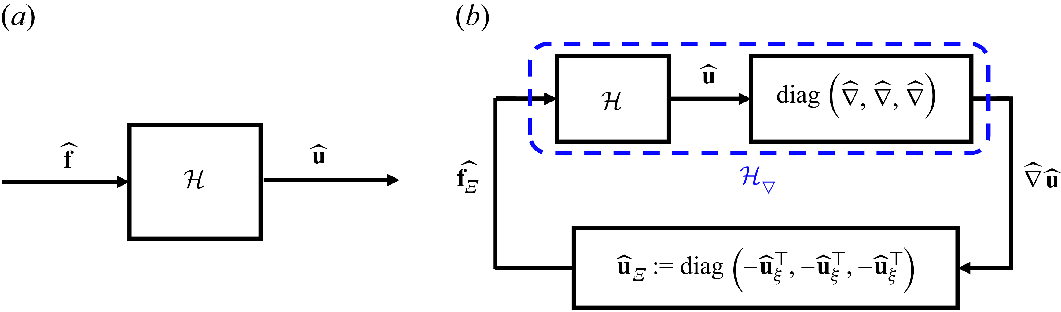
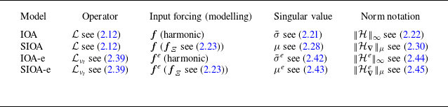


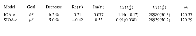


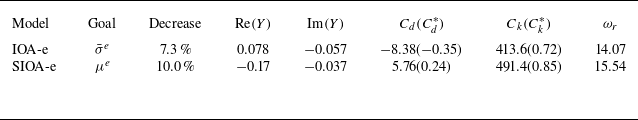


 Open access