


1 Introduction
Near fields of five jets. (a) An accidental oil discharge into sea water from a 50 cm diameter severed pipe at a submarine oil field well-head, where the flow conditions are mostly unknown; the Reynolds number is estimated as $1.4\times 10^{5}$
(Savaş Reference Savaş2012). (b) A well-engineered homogeneous water jet from a 5.1 cm diameter nozzle, where all conditions are known (Yule Reference Yule1978). (c) An opaque homogeneous water jet,
$1.4\times 10^{5}$
(Savaş Reference Savaş2012). (b) A well-engineered homogeneous water jet from a 5.1 cm diameter nozzle, where all conditions are known (Yule Reference Yule1978). (c) An opaque homogeneous water jet, $Re=0.59\times 10^{4}$
(current study). (d,e) Discharging developed turbulent flow of silicone oil in a 1.38 cm diameter pipe (current study): (d) 1 cSt oil jet,
$Re=0.59\times 10^{4}$
(current study). (d,e) Discharging developed turbulent flow of silicone oil in a 1.38 cm diameter pipe (current study): (d) 1 cSt oil jet, $Re=2.41\times 10^{4}$
; and (e) 5 cSt oil jet,
$Re=2.41\times 10^{4}$
; and (e) 5 cSt oil jet, $Re=0.80\times 10^{4}$
. The last three are flows 1, 21 and 24 in table 2, respectively.
$Re=0.80\times 10^{4}$
. The last three are flows 1, 21 and 24 in table 2, respectively.

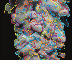
Figure 1 shows examples of the near field within approximately six exit diameters downstream of five jet discharges over a wide range of Reynolds numbers. Figure 1(a) shows a snapshot of the Deepwater Horizon/Macondo Well oil spill in the Gulf of Mexico in April 2010 (McNutt et al.
Reference McNutt, Camilli, Crone, Guthrie, Hsieh, Ryerson, Savaş and Shaffer2012; Savaş Reference Savaş2012; Shaffer et al.
Reference Shaffer, Savaş, Lee and De Vera2015). In this accidental discharge, the upstream conditions in the duct are unknown and the flow conditions in the surrounding water are not well defined. The discharging oil is opaque, hence only the interface between the jet fluid and the surrounding water is visible. The Reynolds number is estimated as $1.4\times 10^{5}$
(Savaş Reference Savaş2012). The visible features at the interface are signatures of the jet turbulence. Any quantitative statements regarding the discharge had to be based on these visible interface features. In contrast, figure 1(b) shows hydrogen-bubble visualization of the near-field cross-sectional view of a laboratory controlled homogeneous water jet egressing from a 5.1 cm diameter nozzle at
$1.4\times 10^{5}$
(Savaş Reference Savaş2012). The visible features at the interface are signatures of the jet turbulence. Any quantitative statements regarding the discharge had to be based on these visible interface features. In contrast, figure 1(b) shows hydrogen-bubble visualization of the near-field cross-sectional view of a laboratory controlled homogeneous water jet egressing from a 5.1 cm diameter nozzle at $Re=9000$
into quiescent water (Yule Reference Yule1978). Evidently, the flow at the discharge plane is uniform and free of turbulence. The unstable cylindrical shear layer develops into a series of vortex rings, the celerity of which can easily be determined from a sequence of images, whence the volume flux, for example, can be deduced. The vortex rings develop streamwise instabilities at higher Reynolds numbers (Savaş & Gollahalli Reference Savaş and Gollahalli1986), but the overall ring structure dominates the near field, which is well understood.
$Re=9000$
into quiescent water (Yule Reference Yule1978). Evidently, the flow at the discharge plane is uniform and free of turbulence. The unstable cylindrical shear layer develops into a series of vortex rings, the celerity of which can easily be determined from a sequence of images, whence the volume flux, for example, can be deduced. The vortex rings develop streamwise instabilities at higher Reynolds numbers (Savaş & Gollahalli Reference Savaş and Gollahalli1986), but the overall ring structure dominates the near field, which is well understood.
Figure 1(c–e), taken from this study and described below, show sample flow images of water and the two silicone oil jets discharging into quiescent water. The Reynolds numbers are high enough that the tripped flows in the discharge tube are developed turbulent flows. That none of the flows shows any orderly ring-like structure as those seen in figure 1(b) may be taken as corroboration of developed turbulent flows in the discharge tube. The homogeneous water jet in figure 1(c) shows the jet–ambient fluid interface clearly. The discharge liquid is rendered opaque, hence only the interface features are visible. The interface is distorted immediately after the fluid leaves the tube and develops into an intricate topology. Shadows created by the dyed jet fluid make the details of the interface clearly visible. Despite the very intricate shape of the interface, there is no indication that it is disconnected. The interface shell lacks the orderliness of figure 1(b), and is more orderly than in figure 1(a). In fact, the spatial statistical uniformity suggests that some features of the interface should be tractable to be able to make quantitative statements about the flow with some acceptable confidence level.
Figure 1(d,e) show 1 cSt and 5 cSt oil jets in water that have visually comparable scales to those in figure 1(c). Reflections off the convex parts of the convoluted interfaces and the surfaces of the detached oil droplets give a starry appearance. As in figure 1(c), flows at the end of the discharge pipe have evidence of developed turbulent flow in the pipe. In stark contrast to the homogeneous jet in figure 1(c), the oil jets exhibit axial striations, or ligaments. Further, instead of the contiguous mushroom-like excursions into the ambient fluid seen in figure 1(c), we now see detached oil droplets in the ambient fluid. It is not clear if there are water droplets in the jet fluid, though. Another feature clearly visible is the underlying large-scale, arrowhead (chevron) structures in the oil jets in figure 1(d,e), which do not seem to have a counterpart in the water jet in figure 1(c). Even though buoyant plumes in a quiescent environment are not expected to meander, one may associate these features with meandering of the jets, however small in amplitude (Hübner Reference Hübner2004). Perhaps unexpectedly, the lower-Reynolds-number flow of the 5 cSt oil jet in figure 1(e) has finer scales than the 1 cSt oil at a higher Reynolds number in figure 1(d). Here again, the scales of these features may be related to the overall characteristics of the discharging jet. It is this aspect of the flows that is the subject matter of this paper.
The self-preserving, asymptotic state of the homogeneous round turbulent jet has been well studied (e.g. Abramovich Reference Abramovich1963; Hinze Reference Hinze1975). Here we sample studies mostly of the near-field behaviour of a jet as it develops from the orifice of discharge. Crow & Champagne (Reference Crow and Champagne1971) present an extensive study on the orderly large coherent structures of well-engineered air jets with clean, uniform initial flow over a range of $0<x/D<16$
, where
$0<x/D<16$
, where $x$
is the downstream distance and
$x$
is the downstream distance and $D$
is the exit diameter. Lau & Fisher (Reference Lau and Fisher1975) concluded that, from hot-wire measurements, the dominant large-scale structure in the first few diameters of a round jet consists of an axial array of toroidal vortices, and as they move downstream they sweep fluid from the high-velocity side of the jet to the other and vice versa. Yule (Reference Yule1978) presents measurements in air and visualization in water in the near field of well-engineered jets where the flow is dominated by toroidal vortices. Bogusławski & Popiel (Reference Bogusławski and Popiel1979) present hot-wire measurements in the extended near field
$D$
is the exit diameter. Lau & Fisher (Reference Lau and Fisher1975) concluded that, from hot-wire measurements, the dominant large-scale structure in the first few diameters of a round jet consists of an axial array of toroidal vortices, and as they move downstream they sweep fluid from the high-velocity side of the jet to the other and vice versa. Yule (Reference Yule1978) presents measurements in air and visualization in water in the near field of well-engineered jets where the flow is dominated by toroidal vortices. Bogusławski & Popiel (Reference Bogusławski and Popiel1979) present hot-wire measurements in the extended near field $(x/D<12)$
of a jet discharging from a fully developed turbulent pipe flow. They present only mean values and report that the highest turbulence intensities occur around
$(x/D<12)$
of a jet discharging from a fully developed turbulent pipe flow. They present only mean values and report that the highest turbulence intensities occur around $(x/D,r/D)\sim (6,1)$
.
$(x/D,r/D)\sim (6,1)$
.
Dimotakis, Miake-Lye & Papantoniou (Reference Dimotakis, Miake-Lye and Papantoniou1983) present laser-induced fluorescence (LIF) measurements in the far field of turbulent water jets over the Reynolds number range of 500 to 10 000 and conclude that large-scale structures, both circular or helical, are persistent in the flow field. Savaş & Gollahalli (Reference Savaş and Gollahalli1986) present schlieren images of the near field of well-engineered propane jets in air, both cold and burning, highlighting the toroidal vortical structures. The smoke wire visualization pictures in figures 5 and 6 of Popiel & Trass (Reference Popiel and Trass1991) show the stark difference between a laminar flow at the jet exit and one that is tripped to turbulence with a screen upstream of the exit. The classical toroidal vortical structures are obliterated by turbulence. Catrakis & Dimotakis (Reference Catrakis and Dimotakis1996) present scalar data, using LIF in water, at $x/D=275$
, where the jet is in its asymptotic, self-similar state. At this measurement location, the ambient fluid may be entrained across the jet, thus rendering the identification a contiguous isosurfaces from side view challenging. In his review article, Dimotakis (Reference Dimotakis2000) discusses the mixing transition that seems to occur at Taylor’s Reynolds number of order 100–140. Hu et al. (Reference Hu, Saga, Kobayashi and Taniguchi2003) present simultaneous particle image velocimetry (PIV) and planar laser-induced fluorescence (PLIF) measurements in the near-nozzle region of a well-engineered jet, essentially duplicating and complementing the work of Yule (Reference Yule1978).
$x/D=275$
, where the jet is in its asymptotic, self-similar state. At this measurement location, the ambient fluid may be entrained across the jet, thus rendering the identification a contiguous isosurfaces from side view challenging. In his review article, Dimotakis (Reference Dimotakis2000) discusses the mixing transition that seems to occur at Taylor’s Reynolds number of order 100–140. Hu et al. (Reference Hu, Saga, Kobayashi and Taniguchi2003) present simultaneous particle image velocimetry (PIV) and planar laser-induced fluorescence (PLIF) measurements in the near-nozzle region of a well-engineered jet, essentially duplicating and complementing the work of Yule (Reference Yule1978).
Westerweel et al. (Reference Westerweel, Hoffman, Fukushima and Hunt2002, Reference Westerweel, Fukushima, Pedersen and Hunt2005, Reference Westerweel, Fukushima, Pedersen and Hunt2009) have presented details of the interface of a homogeneous turbulent water jet of initial diameter $d=1~\text{mm}$
at
$d=1~\text{mm}$
at $Re=2000$
. Westerweel et al. (Reference Westerweel, Hoffman, Fukushima and Hunt2002) present simultaneous PIV and LIF measurements in the water jet, and essentially confirm the results of Catrakis & Dimotakis (Reference Catrakis and Dimotakis1996), that there is a sharp interface between the turbulent and non-turbulent regions of the flow, and irrotational fluid parcels can be found nestled within the rotational turbulent regions. Continuing the work of Westerweel et al. (Reference Westerweel, Hoffman, Fukushima and Hunt2002), based on the analysis of data recorded over
$Re=2000$
. Westerweel et al. (Reference Westerweel, Hoffman, Fukushima and Hunt2002) present simultaneous PIV and LIF measurements in the water jet, and essentially confirm the results of Catrakis & Dimotakis (Reference Catrakis and Dimotakis1996), that there is a sharp interface between the turbulent and non-turbulent regions of the flow, and irrotational fluid parcels can be found nestled within the rotational turbulent regions. Continuing the work of Westerweel et al. (Reference Westerweel, Hoffman, Fukushima and Hunt2002), based on the analysis of data recorded over $60<x/D<100$
, Westerweel et al. (Reference Westerweel, Fukushima, Pedersen and Hunt2005) conclude that the turbulence interface propagates outwards by a small-scale ‘nibbling’ process, which, in turn, implies that large-scale engulfment is not the dominant entrainment mechanism. Westerweel et al. (Reference Westerweel, Fukushima, Pedersen and Hunt2009) reaffirm and further quantify the conclusions in Westerweel et al. (Reference Westerweel, Fukushima, Pedersen and Hunt2005).
$60<x/D<100$
, Westerweel et al. (Reference Westerweel, Fukushima, Pedersen and Hunt2005) conclude that the turbulence interface propagates outwards by a small-scale ‘nibbling’ process, which, in turn, implies that large-scale engulfment is not the dominant entrainment mechanism. Westerweel et al. (Reference Westerweel, Fukushima, Pedersen and Hunt2009) reaffirm and further quantify the conclusions in Westerweel et al. (Reference Westerweel, Fukushima, Pedersen and Hunt2005).
Hunt, Eames & Westerweel (Reference Hunt, Eames and Westerweel2006) developed approximate models at inhomogeneous turbulence interfaces where local structures control the entrainment processes. In their review article of the Euromech 517 Colloquium on Interfacial Processes and Inhomogeneous Turbulence (June 2010), Hunt et al. (Reference Hunt, Eames, da Silva and Westerweel2011) classify interfaces into three categories, one of which is that between turbulent and non-turbulent regions in a flow, similar to the near field of a discharging jet discussed here. They argue that the features at the interface should be observed from their respective reference frames as the flow scales evolve, instead of the laboratory frame. Holzner et al. (Reference Holzner, Liberzon, Nikitin, Kinzelbach and Tsinober2007), who studied the small-scale aspects of flows in proximity of the turbulent/non-turbulent interface, concluded that turbulent entrainment occurs through the viscous forces.
Savaş (Reference Savaş2012) carried out a series of dye flow visualization experiments in water to study the visible flow features in the near field of turbulent jets at Reynolds numbers of $(0.3{-}2.2)\times 10^{5}$
. The large coherent structures at the core of the flow and the smaller eddies at the edge show disparate, independent, length scales, with convection speeds that are more than an order of magnitude apart. Shaffer et al. (Reference Shaffer, Savaş, Lee and De Vera2015) conducted a series of experiments exploring techniques to extract flow rates from video images. They show that a routine application of PIV software to a video of the Deepwater Horizon oil leak jet, a frame of which is shown in figure 1(a), yields velocities that are 10 %–50 % lower than manual measurements of velocities from the advection of the interface features.
$(0.3{-}2.2)\times 10^{5}$
. The large coherent structures at the core of the flow and the smaller eddies at the edge show disparate, independent, length scales, with convection speeds that are more than an order of magnitude apart. Shaffer et al. (Reference Shaffer, Savaş, Lee and De Vera2015) conducted a series of experiments exploring techniques to extract flow rates from video images. They show that a routine application of PIV software to a video of the Deepwater Horizon oil leak jet, a frame of which is shown in figure 1(a), yields velocities that are 10 %–50 % lower than manual measurements of velocities from the advection of the interface features.
The work here focuses on the near field $(x/D<8)$
of homogeneous and immiscible submerged turbulent discharges. Direct flow visualization, schlieren and shadowgraph photography, and PIV are employed simultaneously in various binary combinations. The experimental set-up is described first and the relevant definitions are presented. Then, the homogeneous water jets are presented, followed by the interfacial curvature and length-scale analyses. The oil jets are shown subsequently, followed by the interface scale analysis and oil droplet distribution analyses using Hough transformation. The paper ends with concluding remarks and our parting thoughts.
$(x/D<8)$
of homogeneous and immiscible submerged turbulent discharges. Direct flow visualization, schlieren and shadowgraph photography, and PIV are employed simultaneously in various binary combinations. The experimental set-up is described first and the relevant definitions are presented. Then, the homogeneous water jets are presented, followed by the interfacial curvature and length-scale analyses. The oil jets are shown subsequently, followed by the interface scale analysis and oil droplet distribution analyses using Hough transformation. The paper ends with concluding remarks and our parting thoughts.
Jet fluid properties at $20\,^{\circ }\text{C}$
. Here
$20\,^{\circ }\text{C}$
. Here $\unicode[STIX]{x1D70E}_{a}$
and
$\unicode[STIX]{x1D70E}_{a}$
and $\unicode[STIX]{x1D70E}_{ow}$
are the surface tension in air and interfacial tension in water of the jet liquids, respectively; the
$\unicode[STIX]{x1D70E}_{ow}$
are the surface tension in air and interfacial tension in water of the jet liquids, respectively; the $\unicode[STIX]{x1D70E}_{ow}$
values are estimated using the method suggested by Girifalco & Good (Reference Girifalco and Good1957).
$\unicode[STIX]{x1D70E}_{ow}$
values are estimated using the method suggested by Girifalco & Good (Reference Girifalco and Good1957).

2 Experimental set-up
2.1 Flows
Figure 2 shows the schematics of the experimental set-up employed in the experiments here: the flow loop and the optical layout. The flow loop is shown in figure 2(a). Experiments are conducted in an available $120~\text{cm}\times 240~\text{cm}\times 120~\text{cm}$
(width by length by height) glass water tank at a water level of approximately 105 cm. Jet liquids are discharged into the tank through a vertical smooth copper tube of inner diameter
$120~\text{cm}\times 240~\text{cm}\times 120~\text{cm}$
(width by length by height) glass water tank at a water level of approximately 105 cm. Jet liquids are discharged into the tank through a vertical smooth copper tube of inner diameter $D=1.38~\text{cm}$
, outer diameter of 15.9 mm and length of 42 cm, hence, a length-to-diameter ratio of 30. The end of the tube is machined square. A 30-mesh screen is placed at the entrance to the tube to ensure uniformity at the beginning and also to trip the flow to promote transition to turbulent flow. The tube protrudes from the centre of a 68 cm diameter ground plane. The discharge end of the tube is approximately 50 cm below the free surface of the water tank. The apparatus is a compromise between a desire to achieve high Reynolds numbers (cf.
$D=1.38~\text{cm}$
, outer diameter of 15.9 mm and length of 42 cm, hence, a length-to-diameter ratio of 30. The end of the tube is machined square. A 30-mesh screen is placed at the entrance to the tube to ensure uniformity at the beginning and also to trip the flow to promote transition to turbulent flow. The tube protrudes from the centre of a 68 cm diameter ground plane. The discharge end of the tube is approximately 50 cm below the free surface of the water tank. The apparatus is a compromise between a desire to achieve high Reynolds numbers (cf. $O(10^{5})$
for Deepwater Horizon discharge) and a desire to approximate an unbounded domain, hence the small diameter of the discharge tube.
$O(10^{5})$
for Deepwater Horizon discharge) and a desire to approximate an unbounded domain, hence the small diameter of the discharge tube.
Experimental set-up: (a) flow geometry, cross-sectional illumination and $(x,r)$
coordinate system and the corresponding velocity components
$(x,r)$
coordinate system and the corresponding velocity components $(u_{x},u_{r})$
(side view); (b) schlieren system and camera positions (top view); and (c) illumination for interface visualization (end view).
$(u_{x},u_{r})$
(side view); (b) schlieren system and camera positions (top view); and (c) illumination for interface visualization (end view).

Scope of the experiments. Flow numbers are used for identification in the discussion. Simultaneous imaging modes are indicated as pairs of FV (flow visualization), ScH (schlieren with horizontal knife edge), ScV (schlieren with vertical knife edge), Shd (shadowgraph) and PIV (particle image velocimetry). FR is frame rate (frames per second) and exp. is exposure time. Other definitions are given in § 2.3.

Water and two silicone oils with viscosities of 1 cSt and 5 cSt (Clearco Products Co.: PSF-1cSt octamethyltrisiloxane (trisiloxane) and PSF-5cSt polydimethylsiloxane/PDMS (dimethicone)) are used as the discharge jet fluids. The properties of the liquids are given in table 1. The interfacial tension between the oils and water, $\unicode[STIX]{x1D70E}_{ow}$
, are estimated using the method suggested by Girifalco & Good (Reference Girifalco and Good1957). We note here that the 5 cSt oil has a lower interfacial tension in water than that of the 1 cSt oil. The water jet was coloured with fluorescein sodium salt solution injected upstream into the flow circuit from a dye reservoir (dye reservoir concentration:
$\unicode[STIX]{x1D70E}_{ow}$
, are estimated using the method suggested by Girifalco & Good (Reference Girifalco and Good1957). We note here that the 5 cSt oil has a lower interfacial tension in water than that of the 1 cSt oil. The water jet was coloured with fluorescein sodium salt solution injected upstream into the flow circuit from a dye reservoir (dye reservoir concentration: $1~\text{g}~\text{l}^{-1}$
, 0.1 % by weight). The oil jets are coloured with oil-soluble fluorescent tracing dye (Kingscote Chemicals, no. 506250-RF16, jet fluid concentration 0.07 % by weight). The fluorescein dye used in water experiments was neutralized using common chlorine bleach (Clorox).
$1~\text{g}~\text{l}^{-1}$
, 0.1 % by weight). The oil jets are coloured with oil-soluble fluorescent tracing dye (Kingscote Chemicals, no. 506250-RF16, jet fluid concentration 0.07 % by weight). The fluorescein dye used in water experiments was neutralized using common chlorine bleach (Clorox).
Table 2 lists the experiments of this study. During the flow visualization runs with water jets, the jet fluid is directly supplied from the laboratory supply line. The inherently lower temperature of the supply line water, usually a few degrees Celsius, $\unicode[STIX]{x0394}T=O(5\,^{\circ }\text{C})$
, lower than the ambient temperature, has been sufficient to provide high enough refractive index difference of
$\unicode[STIX]{x0394}T=O(5\,^{\circ }\text{C})$
, lower than the ambient temperature, has been sufficient to provide high enough refractive index difference of $\unicode[STIX]{x0394}n=O(0.001)$
at a low density difference of approximately
$\unicode[STIX]{x0394}n=O(0.001)$
at a low density difference of approximately $\unicode[STIX]{x0394}\unicode[STIX]{x1D70C}\approx 0.0012~\text{g}~\text{cm}^{-3}$
between the jet fluid and the stagnant water in the tank to facilitate schlieren photography. During the PIV runs, a centrifugal pump is employed to generate the water jets by recirculating the seeded water in the tank. For simultaneous PIV and schlieren photography, the supply line, made of copper, was wrapped with an electric heating pad to heat the jet fluid slightly to obtain sufficient refractive index difference for schlieren imaging. During all water jet runs, the flow rate was set by a ball valve and monitored by an industrial-grade turbine flow meter of 1 % accuracy (GPI, model no.: G2S07N09GMA).
$\unicode[STIX]{x0394}\unicode[STIX]{x1D70C}\approx 0.0012~\text{g}~\text{cm}^{-3}$
between the jet fluid and the stagnant water in the tank to facilitate schlieren photography. During the PIV runs, a centrifugal pump is employed to generate the water jets by recirculating the seeded water in the tank. For simultaneous PIV and schlieren photography, the supply line, made of copper, was wrapped with an electric heating pad to heat the jet fluid slightly to obtain sufficient refractive index difference for schlieren imaging. During all water jet runs, the flow rate was set by a ball valve and monitored by an industrial-grade turbine flow meter of 1 % accuracy (GPI, model no.: G2S07N09GMA).
The water jets were operated manually and run continuously, while the oil jets were run on extremely short intervals under computer control to minimize the oil usage. The oil jets were driven by a calibrated gear pump (Pentair Model: Shurflo BBV5) coupled to a microstepper motor (Compumotor). The runs consisted of ramp-up, pre-acquisition steady state, image acquisition and ramp-down phases that are synchronized with the imaging system, all under computer control. The pre-acquisition periods ranged from 4 to 40 s, for the highest and the lowest flow rates in table 2, respectively. These time lags allowed ample time for the oil jets to reach the free surface and spread laterally, reaching steady states before the data acquisition is initiated. The jet oil was contained by a pontoon at the free surface of the tank for quick recovery. The large differences in refractive indices and the immiscibility of water and oils precluded PIV, schlieren and cross-sectional visualization of the oil jets.
2.2 Optics
The schematics of the optical layouts for schlieren/shadowgraph imaging, interface flow visualization, cross-sectional visualization and PIV are all shown jointly in figure 2(b). These imaging techniques could be utilized simultaneously as appropriate.
The classical schlieren layout using two concave mirrors, each of 400 cm focal length and 45 cm diameter, in the Z-configuration is employed here. As shown in figure 2(b), the path of the schlieren system wrapped around the tank by folding the classical Z-configuration using two large front-surface flat mirrors. The beam path is set at $12^{\circ }$
off the normal to the laser sheet in order to allow clear
$12^{\circ }$
off the normal to the laser sheet in order to allow clear $90^{\circ }$
access for the flow visualization cameras. A light-emitting diode (LED) light source is used for illumination (Leica KL 1500LED). The light beam is shaped using a matched achromatic doublet lens pair (Thorlabs MAO:103030-A), a pinhole and a microscope objective. The system is used both with a single knife edge and simultaneously with two orthogonal knife edges after the light beam is split by a cubical beam splitter.
$90^{\circ }$
access for the flow visualization cameras. A light-emitting diode (LED) light source is used for illumination (Leica KL 1500LED). The light beam is shaped using a matched achromatic doublet lens pair (Thorlabs MAO:103030-A), a pinhole and a microscope objective. The system is used both with a single knife edge and simultaneously with two orthogonal knife edges after the light beam is split by a cubical beam splitter.
For PIV, the tank is seeded with silver-coated hollow ceramic spheres of diameter $45~\unicode[STIX]{x03BC}\text{m}$
(Potter Industries Inc., AG-SF-20,
$45~\unicode[STIX]{x03BC}\text{m}$
(Potter Industries Inc., AG-SF-20, $0.8~\text{g}~\text{cm}^{-3}$
). The illumination is done using a 10 W continuous-wave argon-ion laser (American Laser Corp.). PIV data analysis is done using an in-house software package (Sholl & Savaş Reference Sholl and Savaş1997; Ortega, Bristol & Savaş Reference Ortega, Bristol and Savaş2003; Bardet, Peterson & Savaş Reference Bardet, Peterson and Savaş2010; Bardet, Peterson and Savaş Reference Bardet, Peterson and Savaş2018), and post-processing using various commercial software packages. The laser sheet is also used for cross-sectional visualization of the water jets by exciting fluorescent dye in the jet, and the tank had no particles. The immiscibility of oils and water and their mismatched refractive indices precludes cross-sectional viewing of the oil jets in water.
$0.8~\text{g}~\text{cm}^{-3}$
). The illumination is done using a 10 W continuous-wave argon-ion laser (American Laser Corp.). PIV data analysis is done using an in-house software package (Sholl & Savaş Reference Sholl and Savaş1997; Ortega, Bristol & Savaş Reference Ortega, Bristol and Savaş2003; Bardet, Peterson & Savaş Reference Bardet, Peterson and Savaş2010; Bardet, Peterson and Savaş Reference Bardet, Peterson and Savaş2018), and post-processing using various commercial software packages. The laser sheet is also used for cross-sectional visualization of the water jets by exciting fluorescent dye in the jet, and the tank had no particles. The immiscibility of oils and water and their mismatched refractive indices precludes cross-sectional viewing of the oil jets in water.
The interface of the dyed jet fluid was recorded under oblique, nearly collimated illumination from a 1000 lumen LED flashlight set to illuminate the length of ${\sim}10D$
downstream of the discharge orifice. The light was directed so that the refracted light illuminated the jets at
${\sim}10D$
downstream of the discharge orifice. The light was directed so that the refracted light illuminated the jets at $35^{\circ }$
with the horizontal plane as shown in figure 2(c). The flow fields are recorded simultaneously by two high-speed cameras (IDT–X3 and IDT–Y3), in various imaging modes. The cameras both have 1280 pixel
$35^{\circ }$
with the horizontal plane as shown in figure 2(c). The flow fields are recorded simultaneously by two high-speed cameras (IDT–X3 and IDT–Y3), in various imaging modes. The cameras both have 1280 pixel $\times$
1024 pixel native image resolution and are both operated at 1280 pixel
$\times$
1024 pixel native image resolution and are both operated at 1280 pixel $\times$
512 pixel resolution, set at
$\times$
512 pixel resolution, set at $94~\unicode[STIX]{x03BC}\text{m}~\text{pixel}^{-1}$
spatial resolution. They are operated in continuous mode. For simultaneous imaging, the cameras are synchronized in master–slave mode. Operating details are give in table 2.
$94~\unicode[STIX]{x03BC}\text{m}~\text{pixel}^{-1}$
spatial resolution. They are operated in continuous mode. For simultaneous imaging, the cameras are synchronized in master–slave mode. Operating details are give in table 2.
For both water and oil experiments, jets were vertically discharged into the tank of quiescent water. Within the near field that we investigated, the Morton length scale (Morton Reference Morton1959; Turner Reference Turner2012) was sufficiently large to neglect buoyancy effects on the flows for the oil runs listed in table 2.
2.3 Definitions
The coordinate system $(x,r)$
at the central plane of the jets is shown in figure 2. The corresponding velocity components in the plane are
$(x,r)$
at the central plane of the jets is shown in figure 2. The corresponding velocity components in the plane are $\boldsymbol{u}=(u_{x},u_{r})$
. The velocity vector is decomposed as
$\boldsymbol{u}=(u_{x},u_{r})$
. The velocity vector is decomposed as
 $$\begin{eqnarray}\boldsymbol{u}=\boldsymbol{U}+\boldsymbol{u}^{\prime },\end{eqnarray}$$
where $\boldsymbol{U}=(U_{x},U_{r})$
are the time-averaged components and
$\boldsymbol{U}=(U_{x},U_{r})$
are the time-averaged components and $\boldsymbol{u}^{\prime }=(u_{x}^{\prime },u_{r}^{\prime })$
the fluctuating components. Overbars are used to indicate averages. The centreline velocity is denoted as
$\boldsymbol{u}^{\prime }=(u_{x}^{\prime },u_{r}^{\prime })$
the fluctuating components. Overbars are used to indicate averages. The centreline velocity is denoted as $U_{0}(x)$
. For convenience, the radial coordinate
$U_{0}(x)$
. For convenience, the radial coordinate $r$
will at times be substituted by
$r$
will at times be substituted by $y$
.
$y$
.
Table 2 lists the experiments carried out in this study. The main parameter in the experiments is the jet discharge rate $Q$
. The mean discharge velocity
$Q$
. The mean discharge velocity $U$
is written as
$U$
is written as
 $$\begin{eqnarray}U=\frac{4}{\unicode[STIX]{x03C0}}\frac{Q}{D^{2}}.\end{eqnarray}$$
The Reynolds number
 $$\begin{eqnarray}Re=\frac{4}{\unicode[STIX]{x03C0}}\frac{Q}{\unicode[STIX]{x1D708}_{j}D}\end{eqnarray}$$
is based on the jet discharge pipe diameter $D=1.38~\text{cm}$
, the kinematic viscosity of the jet liquid
$D=1.38~\text{cm}$
, the kinematic viscosity of the jet liquid $\unicode[STIX]{x1D708}_{j}$
and the volumetric flow rate
$\unicode[STIX]{x1D708}_{j}$
and the volumetric flow rate $Q$
. The momentum injection rate
$Q$
. The momentum injection rate $M$
is based on the flow rate
$M$
is based on the flow rate $Q$
and the mean discharge velocity
$Q$
and the mean discharge velocity $U$
,
$U$
,
 $$\begin{eqnarray}M=\frac{J}{\unicode[STIX]{x1D70C}_{j}}=QU=\frac{4}{\unicode[STIX]{x03C0}}\frac{Q^{2}}{D^{2}},\end{eqnarray}$$
where $J$
is the jet momentum and
$J$
is the jet momentum and $\unicode[STIX]{x1D70C}_{j}$
the density of the jet liquid. Buoyancy flux
$\unicode[STIX]{x1D70C}_{j}$
the density of the jet liquid. Buoyancy flux $B$
is written as
$B$
is written as
 $$\begin{eqnarray}B=gQ\left(\frac{\unicode[STIX]{x1D70C}_{w}-\unicode[STIX]{x1D70C}_{j}}{\unicode[STIX]{x1D70C}_{w}}\right)=gQ\left(\frac{\unicode[STIX]{x0394}\unicode[STIX]{x1D70C}}{\unicode[STIX]{x1D70C}_{w}}\right),\end{eqnarray}$$
where $g$
is the gravitational acceleration,
$g$
is the gravitational acceleration, $\unicode[STIX]{x1D70C}_{w}$
the density of the ambient water and
$\unicode[STIX]{x1D70C}_{w}$
the density of the ambient water and $\unicode[STIX]{x0394}\unicode[STIX]{x1D70C}=\unicode[STIX]{x1D70C}_{w}-\unicode[STIX]{x1D70C}_{j}$
. The Morton length
$\unicode[STIX]{x0394}\unicode[STIX]{x1D70C}=\unicode[STIX]{x1D70C}_{w}-\unicode[STIX]{x1D70C}_{j}$
. The Morton length $\ell _{M}$
is written as
$\ell _{M}$
is written as
 $$\begin{eqnarray}\displaystyle \frac{\ell _{M}}{D} & = & \displaystyle \frac{M^{3/4}/B^{1/2}}{D}\end{eqnarray}$$
 $$\begin{eqnarray}\displaystyle & = & \displaystyle \left(\frac{\unicode[STIX]{x03C0}}{4}\right)^{1/4}\left(\frac{\unicode[STIX]{x1D70C}_{w}}{\unicode[STIX]{x0394}\unicode[STIX]{x1D70C}}\right)^{1/2}\frac{\unicode[STIX]{x1D708}_{j}}{g^{1/2}D^{3/2}}Re.\end{eqnarray}$$ $\ell _{M}$
is used to gauge the effect of the buoyancy on the oil jets in the near field. Note that
$\ell _{M}$
is used to gauge the effect of the buoyancy on the oil jets in the near field. Note that $\ell _{M}\rightarrow \infty$
for homogeneous jets for which
$\ell _{M}\rightarrow \infty$
for homogeneous jets for which $\unicode[STIX]{x0394}\unicode[STIX]{x1D70C}\approx 0$
.
$\unicode[STIX]{x0394}\unicode[STIX]{x1D70C}\approx 0$
.
The capillary number for the oils jets is written as
 $$\begin{eqnarray}Ca=\frac{\unicode[STIX]{x1D707}_{j}U}{\unicode[STIX]{x1D70E}_{ow}}=\frac{4}{\unicode[STIX]{x03C0}}\frac{\unicode[STIX]{x1D707}_{j}Q}{\unicode[STIX]{x1D70E}_{ow}D^{2}},\end{eqnarray}$$
where $\unicode[STIX]{x1D707}_{j}$
is the dynamic viscosity of the jet fluid. The Weber number is now written as
$\unicode[STIX]{x1D707}_{j}$
is the dynamic viscosity of the jet fluid. The Weber number is now written as
 $$\begin{eqnarray}We=Ca\,Re=\frac{\unicode[STIX]{x1D70C}_{j}U^{2}D}{\unicode[STIX]{x1D70E}_{ow}}=\frac{16}{\unicode[STIX]{x03C0}^{2}}\frac{\unicode[STIX]{x1D70C}_{j}Q^{2}}{\unicode[STIX]{x1D70E}_{ow}D^{3}}.\end{eqnarray}$$
The Richardson number is also defined for reference as
 $$\begin{eqnarray}Ri=\frac{\unicode[STIX]{x0394}\unicode[STIX]{x1D70C}}{\unicode[STIX]{x1D70C}_{w}}\frac{gD}{U^{2}}.\end{eqnarray}$$
The Morton length scale in (2.6) may also be written in terms of the Richardson number as
 $$\begin{eqnarray}\frac{\ell _{M}}{D}=\left(\frac{\unicode[STIX]{x03C0}}{4}\right)^{1/4}Fr^{2}Ri,\end{eqnarray}$$
where the Froude number is defined as $Fr=U/\sqrt{gD}$
.
$Fr=U/\sqrt{gD}$
.
In preparation for discussing turbulence characteristics of the flows, we estimate, at the exit of the discharge tube, the energy dissipation rate $\unicode[STIX]{x1D716}$
(Hinze Reference Hinze1975),
$\unicode[STIX]{x1D716}$
(Hinze Reference Hinze1975),
 $$\begin{eqnarray}\unicode[STIX]{x1D716}=\left(\frac{4}{\unicode[STIX]{x03C0}}\right)^{3}\frac{Q^{3}}{D^{7}},\end{eqnarray}$$
the Kolmogorov length scale $\unicode[STIX]{x1D702}$
and wavenumber
$\unicode[STIX]{x1D702}$
and wavenumber $k_{\unicode[STIX]{x1D702}}$
based on the jet fluid,
$k_{\unicode[STIX]{x1D702}}$
based on the jet fluid,
 $$\begin{eqnarray}\unicode[STIX]{x1D702}=\frac{1}{k_{\unicode[STIX]{x1D702}}}=\left(\frac{\unicode[STIX]{x1D708}_{j}^{3}}{\unicode[STIX]{x1D716}}\right)^{1/4}=Re^{-3/4}D,\end{eqnarray}$$
and the time scale,
 $$\begin{eqnarray}\unicode[STIX]{x1D70F}=\left(\frac{\unicode[STIX]{x1D708}_{j}}{\unicode[STIX]{x1D716}}\right)^{1/2}=\frac{\unicode[STIX]{x03C0}}{4}Re^{-1/2}\frac{D^{3}}{Q}.\end{eqnarray}$$
Table 2 lists $U$
, the Reynolds and Richardson numbers as well the estimates of the Morton lengths and the Kolmogorov scales based on the parameters of the jets. Simultaneous imaging modes are also indicated in the table. The Kolmogorov length scale was used to non-dimensionalize the interface features of the jets: the curvature spectra for the homogeneous water jet runs and droplet size spectra in oil jet experiments.
$U$
, the Reynolds and Richardson numbers as well the estimates of the Morton lengths and the Kolmogorov scales based on the parameters of the jets. Simultaneous imaging modes are also indicated in the table. The Kolmogorov length scale was used to non-dimensionalize the interface features of the jets: the curvature spectra for the homogeneous water jet runs and droplet size spectra in oil jet experiments.
3 Homogeneous water jets
3.1 Flow visualization
3.1.1 Edge visualization
Figure 3 shows sample flow images of fluorescent-dyed homogeneous water jets at three Reynolds numbers. The discharge flows at the tube exit are evidently turbulent, as the interfaces deform well within one diameter of the exit plane (cf. figure 1
b). At the lowest $Re~(5.9\times 10^{3})$
in figure 3(a), the jet–ambient fluid interface is sharply defined; the camera resolution seems to be sufficient to capture all flow surface details. At the intermediate
$Re~(5.9\times 10^{3})$
in figure 3(a), the jet–ambient fluid interface is sharply defined; the camera resolution seems to be sufficient to capture all flow surface details. At the intermediate $Re~(2.39\times 10^{4})$
in figure 3(b), there is a stark decrease in the size of the interface features, as expected with increasing Reynolds number. At the highest
$Re~(2.39\times 10^{4})$
in figure 3(b), there is a stark decrease in the size of the interface features, as expected with increasing Reynolds number. At the highest $Re~(7.22\times 10^{4})$
in figure 3(c), the image has become blurred. There are two obvious reasons for this: the expected size of the turbulence is getting smaller, hence falling out of the spatial resolution of the camera, and the exposure time of the camera is longer than the time scale of the fine-scale interface features, hence blurring the images.
$Re~(7.22\times 10^{4})$
in figure 3(c), the image has become blurred. There are two obvious reasons for this: the expected size of the turbulence is getting smaller, hence falling out of the spatial resolution of the camera, and the exposure time of the camera is longer than the time scale of the fine-scale interface features, hence blurring the images.
Fluorescent water jet experiments: instantaneous images. Flows 1, 3 and 6.

Figure 4 shows averages of 2048 images corresponding to approximately 4 s of the flows in figure 3. The length of the image sequence is not long enough to produce a smooth mean image at the lowest Reynolds number in figure 4(a), which is not unexpected. A study of the corresponding video sequence indicates that the outermost features of the jet fluid move very slowly compared to the features that are deeper in the jet. In fact, some of the jet fluid parcels seem to be nearly stagnant when they have moved away from the jet and into the ambient fluid. The length of the image sequence in figure 4(b) seems to be barely enough to generate a smooth average image. This aspect of the flow is discussed further below in connection with schlieren imaging. The average flow picture in figure 4(c), however, is smooth, indicating that the 4 s of flow at this Reynolds number is sufficiently long to capture a sufficient number of slow-moving jet fluid parcels at the edge of the jet to obtain a meaningful average. The average jet half-spreading angle is estimated from the images to be approximately $12^{\circ }$
at the lowest Reynolds number (flow 1) and approximately
$12^{\circ }$
at the lowest Reynolds number (flow 1) and approximately $8^{\circ }$
at the highest Reynolds number (flow 6). The half-angle decreases monotonically with increasing Reynolds number.
$8^{\circ }$
at the highest Reynolds number (flow 6). The half-angle decreases monotonically with increasing Reynolds number.
Fluorescent water jet experiments: averages of 2048 images. Flows 1, 3 and 6.

3.1.2 Schlieren visualization
Simultaneous flow visualization at the jet edge and schlieren visualization through the jet are available for water jet experiments (table 2). The schlieren images corresponding to those in figure 3 are shown in figure 5, at a slightly lower magnification. As opposed to the edge (shell) visualization, a schlieren image gives an integrated view of the jet along the light path, hence it superimposes all scales of the jet. Figure 5(a,b) show much finer textures than the corresponding images in figure 3, as the result of projecting all flow details across the jet onto a plane. The details get finer as the Reynolds number increases fourfold from figure 5(a) to figure 5(b). A further increase of threefold in $Re$
from figure 5(b) to figure 5(c) is expected to generate even finer details in the flow field in figure 5(c). However, the imaging capability of the camera is not able to capture these finer details. Hence only the large, slower-moving features are recorded in the image.
$Re$
from figure 5(b) to figure 5(c) is expected to generate even finer details in the flow field in figure 5(c). However, the imaging capability of the camera is not able to capture these finer details. Hence only the large, slower-moving features are recorded in the image.
Fluorescent water jet experiments: instantaneous schlieren images corresponding to the panels in figure 3. Flows 1, 3 and 6.

Fluorescent water jet experiments: average of 2048 schlieren images corresponding to the panels in figure 4. Flows 1, 3 and 6.

The schlieren video sequences show nearly stagnant jet fluid parcels at the edge, along with very fast-moving flow features in the interior of the jet. The human eye is able to distinguish these features that are moving at disparate speeds. To some limited degree, features moving at high speed below the canopy of slow-moving outer features can also be identified in the shell visualization videos, but the opacity of the jet fluid limits visible depth past the edge of the jet. One can devise a technique to separate these feature for their speeds through spatiotemporal Fourier transforms. Such an endeavour, however, is beyond the scope of the present discussion.
Similar to figure 4, figure 6 shows the average schlieren pictures corresponding to the flows in figure 5. As in figure 4(a), the number of samples is not large enough to produce a smooth picture at the low Reynolds number flow in figure 6(a). The average half-spreading angles as determined from the schlieren images is slightly lower than those extracted from the direct visualizations in figure 4 (12 $^{\circ }$
versus 10
$^{\circ }$
versus 10 $^{\circ }$
in figures 4(a) and 6(a) and 8
$^{\circ }$
in figures 4(a) and 6(a) and 8 $^{\circ }$
versus 7
$^{\circ }$
versus 7 $^{\circ }$
in figures 4(c) and 6(c)).
$^{\circ }$
in figures 4(c) and 6(c)).
3.1.3 Particle image velocimetry
Figure 7 shows sample simultaneous schlieren and raw PIV images of the homogeneous water jet experiment corresponding to flow 16 at Reynolds number $2.32\times 10^{4}$
in table 2. Also shown is the corresponding instantaneous PIV data as the magnitude of the planar component velocity vector
$2.32\times 10^{4}$
in table 2. Also shown is the corresponding instantaneous PIV data as the magnitude of the planar component velocity vector $\boldsymbol{u}=(u_{x},u_{r})$
, highlighting its spatial variation. Figure 8 shows averaged PIV measurements for flow 16. The data are averaged over 2000 frames. Mean velocity, turbulence intensity, mean vorticity and mean enstrophy are shown. Shown in figure 9 are selected mean velocity profiles for flows 14, 15 and 16. The data are scaled with the local centreline velocity
$\boldsymbol{u}=(u_{x},u_{r})$
, highlighting its spatial variation. Figure 8 shows averaged PIV measurements for flow 16. The data are averaged over 2000 frames. Mean velocity, turbulence intensity, mean vorticity and mean enstrophy are shown. Shown in figure 9 are selected mean velocity profiles for flows 14, 15 and 16. The data are scaled with the local centreline velocity $U_{0}(x)$
and the local jet half-width
$U_{0}(x)$
and the local jet half-width $r_{1/2}(x)$
defined as
$r_{1/2}(x)$
defined as $U_{x}(x,r_{1/2})=U_{0}(x)/2$
. Even in the near field, the jets seem to approach Gaussian profiles at these Reynolds numbers, 6000, 12 000 and 24 000, respectively.
$U_{x}(x,r_{1/2})=U_{0}(x)/2$
. Even in the near field, the jets seem to approach Gaussian profiles at these Reynolds numbers, 6000, 12 000 and 24 000, respectively.
Sample simultaneous schlieren (a) and PIV (b) images and velocity magnitude (c) corresponding to flow 16 in table 2. Here $U=1.83~\text{m}~\text{s}^{-1}$
. The end of the discharge tube is visible on the left in the images.
$U=1.83~\text{m}~\text{s}^{-1}$
. The end of the discharge tube is visible on the left in the images.

Average velocity, turbulence intensity, vorticity and enstrophy in homogeneous water jet: $Re=24\,000$
. Flow 16 in table 2,
$Re=24\,000$
. Flow 16 in table 2, $U=1.83~\text{m}~\text{s}^{-1}$
and
$U=1.83~\text{m}~\text{s}^{-1}$
and $U/D=133~\text{s}^{-1}$
.
$U/D=133~\text{s}^{-1}$
.

PIV average velocity profiles in homogeneous water jets. Flows 14, 15 and 16.

3.2 Curvature analysis
Image processing for curvature analysis begins with intensity remapping to stretch the dynamic range of the images to 8-bit level. Then, the images underwent the Canny edge detection process (Canny Reference Canny1986). The scaled image is first smoothed through a $5\times 5$
Gaussian convolution kernel to arrive at smoothed images
$5\times 5$
Gaussian convolution kernel to arrive at smoothed images $I_{f}$
in order to reduce the occurrence of noise-induced false edges. A sample of the smoothed images is shown in figure 10(a). The round Sobel edge detection operation (Sobel & Feldman Reference Sobel, Feldman, Duda and Hart1968) is carried out on the filtered image,
$I_{f}$
in order to reduce the occurrence of noise-induced false edges. A sample of the smoothed images is shown in figure 10(a). The round Sobel edge detection operation (Sobel & Feldman Reference Sobel, Feldman, Duda and Hart1968) is carried out on the filtered image, $I_{f}$
, which employs a centred finite difference approximation,
$I_{f}$
, which employs a centred finite difference approximation, $S_{h}$
and
$S_{h}$
and $S_{v}$
, for the first derivative in the vertical and horizontal directions to calculate image gradient. The gradient vector
$S_{v}$
, for the first derivative in the vertical and horizontal directions to calculate image gradient. The gradient vector $\boldsymbol{G}$
in the filtered image is calculated via convolution as
$\boldsymbol{G}$
in the filtered image is calculated via convolution as
 $$\begin{eqnarray}\boldsymbol{G}=(G_{h},G_{v})=(S_{h},S_{v})\circ I_{f}.\end{eqnarray}$$
Finally, the magnitude $I_{g}$
and the direction
$I_{g}$
and the direction $\unicode[STIX]{x1D6E9}$
of the image gradient vector are constructed as, respectively,
$\unicode[STIX]{x1D6E9}$
of the image gradient vector are constructed as, respectively,
 $$\begin{eqnarray}I_{g}=|\boldsymbol{G}|=\sqrt{G_{h}^{2}+G_{v}^{2}}\quad \text{and}\quad \unicode[STIX]{x1D6E9}=\text{atan}(G_{v}/G_{h}).\end{eqnarray}$$
This image gradient magnitude $I_{g}$
is used to determine the locations of edges in an image, a sample of which is shown in figure 10(b). The direction of the gradient vector
$I_{g}$
is used to determine the locations of edges in an image, a sample of which is shown in figure 10(b). The direction of the gradient vector $\unicode[STIX]{x1D6E9}$
is used for the non-maximum suppression process. The angle
$\unicode[STIX]{x1D6E9}$
is used for the non-maximum suppression process. The angle $\unicode[STIX]{x1D6E9}$
is rounded to the closest
$\unicode[STIX]{x1D6E9}$
is rounded to the closest $45^{\circ }$
increment: i.e.
$45^{\circ }$
increment: i.e. $0^{\circ }$
,
$0^{\circ }$
, $45^{\circ }$
,
$45^{\circ }$
, $90^{\circ }$
or
$90^{\circ }$
or $135^{\circ }$
. At a given pixel, the neighbours in directions perpendicular to the gradient direction are checked. If the pixel’s gradient magnitude is greater than those of its neighbours, it is preserved and the neighbours are negated; or vice versa if the opposite occurs. The image gradient was binarized using the Otsu thresholding method (Otsu Reference Otsu1979; Sezgin & Sankur Reference Sezgin and Sankur2004). The Otsu thresholding method is an easily implemented cluster-based algorithm that selects threshold levels from the histograms of image segments maximizing the separability of the resultant classes in grey levels. The images are then skeletonized through a morphological thinning process as discussed in Jang & Chin (Reference Jang and Chin1990), a sample of which is shown in figure 10(c), along with a detailed segment in figure 10(d). These edges are further examined to reject branches and segments shorter than 10 pixels.
$135^{\circ }$
. At a given pixel, the neighbours in directions perpendicular to the gradient direction are checked. If the pixel’s gradient magnitude is greater than those of its neighbours, it is preserved and the neighbours are negated; or vice versa if the opposite occurs. The image gradient was binarized using the Otsu thresholding method (Otsu Reference Otsu1979; Sezgin & Sankur Reference Sezgin and Sankur2004). The Otsu thresholding method is an easily implemented cluster-based algorithm that selects threshold levels from the histograms of image segments maximizing the separability of the resultant classes in grey levels. The images are then skeletonized through a morphological thinning process as discussed in Jang & Chin (Reference Jang and Chin1990), a sample of which is shown in figure 10(c), along with a detailed segment in figure 10(d). These edges are further examined to reject branches and segments shorter than 10 pixels.
The resulting edge image is used for curvature analysis below, a sample of which is shown in figure 11 for the water jet at $Re=6.22\times 10^{3}$
. To analyse the curvature of the segments, the curves were parametrized by their
$Re=6.22\times 10^{3}$
. To analyse the curvature of the segments, the curves were parametrized by their $[x,y]$
position, as a function of the position along the length of the segment,
$[x,y]$
position, as a function of the position along the length of the segment, $s$
, beginning at the initial pixel,
$s$
, beginning at the initial pixel, $P_{0}$
, of the edge curve
$P_{0}$
, of the edge curve $s(P_{0})=0$
or
$s(P_{0})=0$
or $s(x_{0},y_{0})=0$
. The value of
$s(x_{0},y_{0})=0$
. The value of $s$
was used to parametrize both the
$s$
was used to parametrize both the $x_{n}$
and
$x_{n}$
and $y_{n}$
for a given pixel,
$y_{n}$
for a given pixel, $P_{n}$
. Distances between each of the following pixels, in order, was calculated:
$P_{n}$
. Distances between each of the following pixels, in order, was calculated:
 $$\begin{eqnarray}ds_{n}(P_{n})=ds(P_{n-1}-P_{n})=\sqrt{(x_{n-1}-x_{n})^{2}+(y_{n-1}-y_{n})^{2}}.\end{eqnarray}$$
Note that $ds_{n}=1$
or
$ds_{n}=1$
or $\sqrt{2}$
pixel. This definition of
$\sqrt{2}$
pixel. This definition of $s$
leads to non-uniforming spacing between the values of
$s$
leads to non-uniforming spacing between the values of $s_{n}$
:
$s_{n}$
:
 $$\begin{eqnarray}s_{n}=s(P_{n})=\mathop{\sum }_{i=0}^{n}ds_{i}(P_{i}).\end{eqnarray}$$
Per curve segment, a vector of these discrete $(x_{n},y_{n})$
is constructed. Each of these was treated as a sampling of the function
$(x_{n},y_{n})$
is constructed. Each of these was treated as a sampling of the function
 $$\begin{eqnarray}\boldsymbol{X}(s_{n})=(X(s_{n}),Y(s_{n}))=(x_{n},y_{n})=\boldsymbol{x}_{n}\end{eqnarray}$$
at non-uniform sampling points along the length $s$
.
$s$
.
Sample homogeneous jet image demonstrating edge detection process: $Re=1.20\times 10^{4}$
. (a) A sample image from the video sequence after Gaussian filtering; (b) its intensity gradient magnitude; (c) thinned edges; and (d) details of edges from panel (c).
$Re=1.20\times 10^{4}$
. (a) A sample image from the video sequence after Gaussian filtering; (b) its intensity gradient magnitude; (c) thinned edges; and (d) details of edges from panel (c).

All curves found after the segmentation process for a homogeneous turbulent jet of $Re=6.22\times 10^{3}$
. Colour is added to show segments.
$Re=6.22\times 10^{3}$
. Colour is added to show segments.

The sizes of the edge curve segments analysed range from $O(10)$
to
$O(10)$
to $O(10^{2})$
data points in length. A cubic smoothing spline is used to fit
$O(10^{2})$
data points in length. A cubic smoothing spline is used to fit $\boldsymbol{x}=(x,y)$
with respect to position along the length of the segment. The process allows the splines to depart from the data points with a weighted penalization, trading off between the smoothness of the function versus the approximation of the data point values by the curve. This is accomplished by finding
$\boldsymbol{x}=(x,y)$
with respect to position along the length of the segment. The process allows the splines to depart from the data points with a weighted penalization, trading off between the smoothness of the function versus the approximation of the data point values by the curve. This is accomplished by finding $({\mathcal{X}},{\mathcal{Y}})$
that minimized the functionals
$({\mathcal{X}},{\mathcal{Y}})$
that minimized the functionals $({\mathcal{L}}_{x},{\mathcal{L}}_{y})$
:
$({\mathcal{L}}_{x},{\mathcal{L}}_{y})$
:
 $$\begin{eqnarray}({\mathcal{L}}_{x},{\mathcal{L}}_{y})=p\mathop{\sum }_{i}[(x_{i}-{\mathcal{X}}(s_{i}))^{2},(y_{i}-{\mathcal{Y}}(s_{i}))^{2}]+(1-p)\int \left[\left({\displaystyle \frac{\text{d}^{2}{\mathcal{X}}}{\text{d}s^{2}}}\right)^{2},\left({\displaystyle \frac{\text{d}^{2}{\mathcal{Y}}}{\text{d}s^{2}}}\right)^{2}\right]\,\text{d}s.\end{eqnarray}$$
This is a variant of the functional described in Reinsch (Reference Reinsch1967). A smoothing parameter $p$
, which ranges over
$p$
, which ranges over $[0,1]$
, is employed to tune this tradeoff. In the case of
$[0,1]$
, is employed to tune this tradeoff. In the case of $p=0$
, the result prioritizes smoothing, with a steep penalty for any oscillations, and return a linear least-squares estimate of a fit, while
$p=0$
, the result prioritizes smoothing, with a steep penalty for any oscillations, and return a linear least-squares estimate of a fit, while $p=1$
returns an interpolating cubic spline. Using a cubic interpolating spline for
$p=1$
returns an interpolating cubic spline. Using a cubic interpolating spline for $x(s_{i})$
and
$x(s_{i})$
and $y(s_{i})$
requires the spline to match the value at each point, which generates spurious oscillations of the curvature along a segment. For all segments,
$y(s_{i})$
requires the spline to match the value at each point, which generates spurious oscillations of the curvature along a segment. For all segments, $p=1/2$
is used, which provides sufficient damping of oscillations in the derivatives of the fit while accurately capturing the path of the data points. The segment is then resampled at equispaced points along the lengths of the curve using the cubic smoothing spline fit. The number of points used to represent the segment is preserved.
$p=1/2$
is used, which provides sufficient damping of oscillations in the derivatives of the fit while accurately capturing the path of the data points. The segment is then resampled at equispaced points along the lengths of the curve using the cubic smoothing spline fit. The number of points used to represent the segment is preserved.
The first and second derivatives, $({\mathcal{X}}^{\prime },{\mathcal{Y}}^{\prime })$
and
$({\mathcal{X}}^{\prime },{\mathcal{Y}}^{\prime })$
and $({\mathcal{X}}^{\prime \prime },{\mathcal{Y}}^{\prime \prime })$
, with respect to
$({\mathcal{X}}^{\prime \prime },{\mathcal{Y}}^{\prime \prime })$
, with respect to $s$
are calculated using five-point centred finite difference kernels (Abramowitz & Stegun Reference Abramowitz and Stegun1964). The two endpoints on each side of the segment were treated with a non-centred finite difference scheme while matching the accuracy of the centre scheme. The curvature along the segment is evaluated as
$s$
are calculated using five-point centred finite difference kernels (Abramowitz & Stegun Reference Abramowitz and Stegun1964). The two endpoints on each side of the segment were treated with a non-centred finite difference scheme while matching the accuracy of the centre scheme. The curvature along the segment is evaluated as
 $$\begin{eqnarray}\unicode[STIX]{x1D705}(s_{i})={\displaystyle \frac{{\mathcal{X}}_{i}^{\prime }{\mathcal{Y}}_{i}^{\prime \prime }-{\mathcal{Y}}_{i}^{\prime }{\mathcal{X}}_{i}^{\prime \prime }}{({\mathcal{X}}_{i}^{\prime 2}+{\mathcal{Y}}_{i}^{\prime 2})^{3/2}}}.\end{eqnarray}$$
Figure 12 illustrates the stages in analysing segments for a homogeneous water jet of $Re=6.22\times 10^{3}$
. Per segment, the discrete curvature measurement along its length is converted to the measure of the magnitude of the curvature in the segment with respect to the wavenumbers at which they occur. This is done by taking the discrete Fourier transform of the curvature vector for a segment
$Re=6.22\times 10^{3}$
. Per segment, the discrete curvature measurement along its length is converted to the measure of the magnitude of the curvature in the segment with respect to the wavenumbers at which they occur. This is done by taking the discrete Fourier transform of the curvature vector for a segment $\unicode[STIX]{x1D705}(s_{i})$
. The corresponding wavenumber is constructed with the inverse of the length between sampling points,
$\unicode[STIX]{x1D705}(s_{i})$
. The corresponding wavenumber is constructed with the inverse of the length between sampling points, $\unicode[STIX]{x0394}s$
, with the number of sampling points,
$\unicode[STIX]{x0394}s$
, with the number of sampling points, $N$
. The value of
$N$
. The value of $\unicode[STIX]{x0394}s$
is constant per segment, as they are sampled at equispaced distances along the length of the segment:
$\unicode[STIX]{x0394}s$
is constant per segment, as they are sampled at equispaced distances along the length of the segment:
 $$\begin{eqnarray}\displaystyle & \displaystyle k_{j}=j{\displaystyle \frac{N}{\unicode[STIX]{x0394}s}},\quad 0\leqslant j\leqslant {\displaystyle \frac{N}{2}}, & \displaystyle\end{eqnarray}$$
 $$\begin{eqnarray}\displaystyle & \displaystyle {\mathcal{K}}_{j}={\mathcal{K}}(k_{j})={\mathcal{F}}(\unicode[STIX]{x1D705}(s_{j})). & \displaystyle\end{eqnarray}$$
The amplitude of the curvature at a wavenumber is found by taking the length of the complex value of ${\mathcal{K}}(k)$
normalized by the length of the vector,
${\mathcal{K}}(k)$
normalized by the length of the vector, $N$
. If
$N$
. If $N$
is even, the highest mode is excluded:
$N$
is even, the highest mode is excluded:
 $$\begin{eqnarray}\displaystyle & \displaystyle \widetilde{{\mathcal{P}}}_{j}={\displaystyle \frac{|{\mathcal{K}}_{j}|}{N}}, & \displaystyle\end{eqnarray}$$
 $$\begin{eqnarray}\displaystyle & \displaystyle {\mathcal{P}}_{j}=\left\{\begin{array}{@{}ll@{}}\widetilde{{\mathcal{P}}}_{j},\quad & j=0,\\ \widetilde{{\mathcal{P}}}_{j}\times 2,\quad & 0<j\leqslant N/2.\end{array}\right. & \displaystyle\end{eqnarray}$$
Here ${\mathcal{P}}_{j}$
corresponds to the amplitude of the curvature signal at the wavenumber
${\mathcal{P}}_{j}$
corresponds to the amplitude of the curvature signal at the wavenumber $k_{j}$
. This process is done for each segment in the image that exists in the region between
$k_{j}$
. This process is done for each segment in the image that exists in the region between $1\leqslant x/D\leqslant 8$
downstream. Per homogeneous jet run, the results reported are a collection of all segments captured through all the images used for that run.
$1\leqslant x/D\leqslant 8$
downstream. Per homogeneous jet run, the results reported are a collection of all segments captured through all the images used for that run.
Sample homogeneous jet image demonstrating curvature analysis for $Re=6.22\times 10^{3}$
. (a) Full view of image with a sample edge segment and (b) analysis. The edge segment in (a) is reflected horizontally and reproduced in the first panel of (b). The second and third panels (clockwise) of (b) show
$Re=6.22\times 10^{3}$
. (a) Full view of image with a sample edge segment and (b) analysis. The edge segment in (a) is reflected horizontally and reproduced in the first panel of (b). The second and third panels (clockwise) of (b) show $x(s)$
and
$x(s)$
and $y(s)$
, and spline fits and their derivatives, respectively. Finally, the last panel shows the curvature from (3.7), along the length of the edge segment above it where one can easily match the corresponding features in both frames.
$y(s)$
, and spline fits and their derivatives, respectively. Finally, the last panel shows the curvature from (3.7), along the length of the edge segment above it where one can easily match the corresponding features in both frames.

Figure 13 shows the results of the curvature density calculations of the turbulent water jets. The curvature $|\unicode[STIX]{x1D705}|$
is scaled with the local Kolmogorov wavenumber
$|\unicode[STIX]{x1D705}|$
is scaled with the local Kolmogorov wavenumber $k_{\unicode[STIX]{x1D702}}(x)$
and plotted against the wavenumber, which is non-dimensionalized again with the Kolmogorov wavenumber and further scaled with
$k_{\unicode[STIX]{x1D702}}(x)$
and plotted against the wavenumber, which is non-dimensionalized again with the Kolmogorov wavenumber and further scaled with $Re^{3/4}$
. Recalling the definition in (2.12), the wavenumber scaling simply amounts to writing
$Re^{3/4}$
. Recalling the definition in (2.12), the wavenumber scaling simply amounts to writing $kD$
. The data are sorted into 35 wavenumber bins and subsequently averaged to construct the curvature histograms of Fourier amplitudes for each Reynolds number in figure 13. The horizontal dashed line at
$kD$
. The data are sorted into 35 wavenumber bins and subsequently averaged to construct the curvature histograms of Fourier amplitudes for each Reynolds number in figure 13. The horizontal dashed line at $|\unicode[STIX]{x1D705}|/k_{\unicode[STIX]{x1D702}}=0.10$
in the figure marks the boundary of where the period of the spectral component is spread over six or fewer pixels in images. Resulting trends below this threshold should be viewed with caution.
$|\unicode[STIX]{x1D705}|/k_{\unicode[STIX]{x1D702}}=0.10$
in the figure marks the boundary of where the period of the spectral component is spread over six or fewer pixels in images. Resulting trends below this threshold should be viewed with caution.
Curvature density spectrum $|\unicode[STIX]{x1D705}|~(\text{m}^{-1})$
with respect to wavenumber normalized by the pipe Kolmogorov wavenumber for the homogeneous jet experiments investigated. The horizontal dashed line corresponds to soft cutoff to the spatial resolution of the curvature signal.
$|\unicode[STIX]{x1D705}|~(\text{m}^{-1})$
with respect to wavenumber normalized by the pipe Kolmogorov wavenumber for the homogeneous jet experiments investigated. The horizontal dashed line corresponds to soft cutoff to the spatial resolution of the curvature signal.

The packing of the data gives insight into which wavenumbers the results clustered around. The highest amplitudes occur at lower wavenumbers, those easily picked out by the naked eye in the flow images. Figure 13 also illustrates the prevalence of high wavenumbers with relatively small Fourier amplitudes. Thus, along the length of segments in figure 11, low wavenumbers are manifested as high-amplitude curves and high wavenumbers as low-amplitude curves. Beyond the dominant amplitudes, the curvature amplitudes at higher wavenumbers fall off at a rate of $-7/3$
and at the highest wavenumbers with
$-7/3$
and at the highest wavenumbers with $-5/3$
.
$-5/3$
.
The analysis of these results indicates that curvatures are relaxed at rates dependent on their magnitude, with higher-curvature features not being sustained as long as lower-curvature features. Smaller eddies decay faster than larger eddies, a quintessential feature of turbulent flows. These results, in general, may suffer from quantification noise introduced by the resolution of the image, where a line must be represented as discrete steps in pixel locations. The smooth spline fitting was used to inhibit this source of error, but occurrences of cusps in the segments as they are detected by the algorithm may not be physically indicative of the continuous features. A scheme to validate or reject cusps would be desirable to help mitigate inaccuracies in the edge tracing.
3.3 Interfacial length scale
Interface length scales are extracted from the jet images. The images, however, suffer from spatially inhomogeneous illumination along the axis of the jet. To mitigate any bias from the waning illumination intensity, a contrast-limited adaptive histogram equalization (CLAHE) technique is employed (Pizer et al. Reference Pizer, Amburn, Austin, Cromartie, Geselowitz, Greer, ter Haar Romeny, Zimmerman and Zuiderveld1987). Figure 14 shows sample results after the CLAHE operation on the different Reynolds-number homogeneous jets. Note that the nearly uniform dark backgrounds in the original images become rather noisy due to local amplification during CLAHE.
Sample images of CLAHE on fluorescent homogeneous water jets.

Figure 15 illustrates the procedure to extract length scales from the images. The sample interrogation tile in figure 15(a), 256 pixel $\times$
256 pixel, is at
$\times$
256 pixel, is at $x/D=3.42$
downstream from the exit of the pipe of the jet for
$x/D=3.42$
downstream from the exit of the pipe of the jet for $Re=25.0\times 10^{3}$
. The intensity field
$Re=25.0\times 10^{3}$
. The intensity field $I(x,y)$
is shown in figure 15(b) in isometric form. To prevent leakage in the two-dimensional (2-D) signal as it is taken into the Fourier domain, a 2-D Tukey window (tapered cosine window) is applied to the interrogation region to construct a periodic boundary, which is constructed by extending the one-dimensional (1-D) Tukey window (Tukey Reference Tukey and Harris1967). Thus windowed image intensity is now
$I(x,y)$
is shown in figure 15(b) in isometric form. To prevent leakage in the two-dimensional (2-D) signal as it is taken into the Fourier domain, a 2-D Tukey window (tapered cosine window) is applied to the interrogation region to construct a periodic boundary, which is constructed by extending the one-dimensional (1-D) Tukey window (Tukey Reference Tukey and Harris1967). Thus windowed image intensity is now $I_{w}(x,y)$
.
$I_{w}(x,y)$
.
Processing steps for the interrogation region of the homogeneous jet at $Re=25.0\times 10^{3}$
at
$Re=25.0\times 10^{3}$
at $x/d=3.42$
. (a) A sample interrogation region along the jet; (b) raw intensity array; (c) interrogation tile’s intensity values after 2-D Tukey windowing; (d) the results of the 2-D autocorrelation function (ACF) of the windowed tile; and (e) the cross-stream (X-stream, red dashed line) and streamwise (black dashed line) osculating parabolas (osc. p.) to the ACF (solid lines with the same respective colour).
$x/d=3.42$
. (a) A sample interrogation region along the jet; (b) raw intensity array; (c) interrogation tile’s intensity values after 2-D Tukey windowing; (d) the results of the 2-D autocorrelation function (ACF) of the windowed tile; and (e) the cross-stream (X-stream, red dashed line) and streamwise (black dashed line) osculating parabolas (osc. p.) to the ACF (solid lines with the same respective colour).

Interfacial length-scale results for water jet: (a) length ratio $\unicode[STIX]{x1D706}_{x}/\unicode[STIX]{x1D706}_{y}$
, (b) mean length scale
$\unicode[STIX]{x1D706}_{x}/\unicode[STIX]{x1D706}_{y}$
, (b) mean length scale $\unicode[STIX]{x1D706}=(\unicode[STIX]{x1D706}_{x}+\unicode[STIX]{x1D706}_{y})/2$
and (c) interface length scaled with the Taylor microscale
$\unicode[STIX]{x1D706}=(\unicode[STIX]{x1D706}_{x}+\unicode[STIX]{x1D706}_{y})/2$
and (c) interface length scaled with the Taylor microscale $\unicode[STIX]{x1D706}/\tilde{\unicode[STIX]{x1D706}}_{g}$
.
$\unicode[STIX]{x1D706}/\tilde{\unicode[STIX]{x1D706}}_{g}$
.

The windowing process reduces the largest length scale that can be detected by this, akin to the Taylor microscale analysis. As the radius of the jet is contained in the interrogation region for the initial steps, all scales that exist within are able to be estimated. Interrogation regions further downstream of the jet do not capture the whole jet profile: this allows features of comparable scales to not be effectively detected. The Tukey windowed form of the intensity data in figure 15(b) is shown in figure 15(c).
The autocorrelation of the windowed region is calculated using 2-D Fourier analysis,
 $$\begin{eqnarray}R(\bar{{\mathcal{X}}})={\mathcal{F}}^{-1}({\mathcal{I}}(\bar{k}){\mathcal{I}}^{^{\ast }}(\bar{k})),\end{eqnarray}$$
where ${\mathcal{I}}(\bar{k})={\mathcal{F}}(I_{w}(\bar{x}))$
and
${\mathcal{I}}(\bar{k})={\mathcal{F}}(I_{w}(\bar{x}))$
and $\bar{k}=[k_{x},k_{y}]$
is the wavevector. The autocorrelation
$\bar{k}=[k_{x},k_{y}]$
is the wavevector. The autocorrelation $R(\bar{{\mathcal{X}}})$
is shown in figure 15(d). The second derivatives of
$R(\bar{{\mathcal{X}}})$
is shown in figure 15(d). The second derivatives of $R(\bar{{\mathcal{X}}})$
at the centre peak are used to estimate the streamwise and cross-stream length scales
$R(\bar{{\mathcal{X}}})$
at the centre peak are used to estimate the streamwise and cross-stream length scales $(\unicode[STIX]{x1D706}_{x},\unicode[STIX]{x1D706}_{y})$
, respectively. These derivatives are evaluated using a centred five-point finite difference kernel (Abramowitz & Stegun Reference Abramowitz and Stegun1964). The length scale is written as
$(\unicode[STIX]{x1D706}_{x},\unicode[STIX]{x1D706}_{y})$
, respectively. These derivatives are evaluated using a centred five-point finite difference kernel (Abramowitz & Stegun Reference Abramowitz and Stegun1964). The length scale is written as
 $$\begin{eqnarray}(\unicode[STIX]{x1D706}_{x},\unicode[STIX]{x1D706}_{y})=\left(\left[\frac{1}{2}\left|\frac{\unicode[STIX]{x2202}^{2}R(0,0)}{\unicode[STIX]{x2202}{\mathcal{X}}^{2}}\right|\right]^{-1/2},\left[\frac{1}{2}\left|\frac{\unicode[STIX]{x2202}^{2}R(0,0)}{\unicode[STIX]{x2202}{\mathcal{Y}}^{2}}\right|\right]^{-1/2}\right),\end{eqnarray}$$
which amounts to fitting two orthogonal osculating parabolas at the peak $R(0,0)=1$
in figure 15(e). The average of the longitudinal and transverse length scales,
$R(0,0)=1$
in figure 15(e). The average of the longitudinal and transverse length scales,
 $$\begin{eqnarray}\unicode[STIX]{x1D706}={\textstyle \frac{1}{2}}(\unicode[STIX]{x1D706}_{x}+\unicode[STIX]{x1D706}_{y}),\end{eqnarray}$$
is reported to give insight into the growth trend of the structures in the case of the homogeneous jet. The 256 pixel $\times$
256 pixel interrogation tiles were stepped along the axis of the jet in 64 pixel increments, the first one centred at
$\times$
256 pixel interrogation tiles were stepped along the axis of the jet in 64 pixel increments, the first one centred at $x/D=3.42$
, and the last one at
$x/D=3.42$
, and the last one at $x/D=7.54$
, for a range of
$x/D=7.54$
, for a range of $Re\approx 6000{-}45\,000$
.
$Re\approx 6000{-}45\,000$
.
Figure 16 shows the interface length scale for the water jets: the length-scale ratio $\unicode[STIX]{x1D706}_{x}/\unicode[STIX]{x1D706}_{y}$
in figure 16(a) and the average interfacial length scale
$\unicode[STIX]{x1D706}_{x}/\unicode[STIX]{x1D706}_{y}$
in figure 16(a) and the average interfacial length scale $\unicode[STIX]{x1D706}$
in figure 16(b). The ratio
$\unicode[STIX]{x1D706}$
in figure 16(b). The ratio $\unicode[STIX]{x1D706}_{x}/\unicode[STIX]{x1D706}_{y}$
is virtually unity, regardless of
$\unicode[STIX]{x1D706}_{x}/\unicode[STIX]{x1D706}_{y}$
is virtually unity, regardless of $x/D$
and Reynolds number, which attests to the isotropy at the interface. Figure 16(c) shows the ratio of the interface scale to the local Taylor microscale,
$x/D$
and Reynolds number, which attests to the isotropy at the interface. Figure 16(c) shows the ratio of the interface scale to the local Taylor microscale, $\unicode[STIX]{x1D706}/\tilde{\unicode[STIX]{x1D706}}_{g}$
, where the local Taylor microscale
$\unicode[STIX]{x1D706}/\tilde{\unicode[STIX]{x1D706}}_{g}$
, where the local Taylor microscale $\tilde{\unicode[STIX]{x1D706}}_{g}$
is estimated from the root-mean-square fluctuations of shear strain rates deduced from the PIV measurements (Pope Reference Pope2000). In figure 16(a), a monotonic increase with
$\tilde{\unicode[STIX]{x1D706}}_{g}$
is estimated from the root-mean-square fluctuations of shear strain rates deduced from the PIV measurements (Pope Reference Pope2000). In figure 16(a), a monotonic increase with $x/D$
of the average interfacial length scales is seen for all Reynolds numbers. The rate at which these scales increase is seen to be inversely related to the jet Reynolds number. The ratio
$x/D$
of the average interfacial length scales is seen for all Reynolds numbers. The rate at which these scales increase is seen to be inversely related to the jet Reynolds number. The ratio $\unicode[STIX]{x1D706}/\tilde{\unicode[STIX]{x1D706}}_{g}$
is uniform over the measurement domain and monotonically increases with Reynolds number at a diminishing rate.
$\unicode[STIX]{x1D706}/\tilde{\unicode[STIX]{x1D706}}_{g}$
is uniform over the measurement domain and monotonically increases with Reynolds number at a diminishing rate.
4 Oil jets in water
4.1 Oil jets: 1 cSt
4.1.1 Edge visualization
Figure 17 shows sample flow images for 1 cSt oil jets at three Reynolds numbers: $0.4\times 10^{4}$
,
$0.4\times 10^{4}$
, $2.4\times 10^{4}$
and
$2.4\times 10^{4}$
and $4.0\times 10^{4}$
. The flow in the tube upstream of the jet exit is expected to be transitional, since it is tripped by a screen mesh, and the Reynolds number is approximately 4000. The combined effects of the immiscibility of the jet and ambient liquids, augmented by the expected transitional nature of the discharge flow, results in large detached parcels of oil after a short distance of undulations. As the Reynolds number is increased by sixfold in figure 17(b), the discharge tube length becomes adequate to achieve turbulent flow at the exit of the tube. The flow leaving the tube now shows streamwise features, the wall signatures of the turbulent flow in the pipe. Further increase in the Reynolds number in figure 17(c) results in finer details, as expected, both on the jet surface and in the size distribution of the detached oil droplets.
$4.0\times 10^{4}$
. The flow in the tube upstream of the jet exit is expected to be transitional, since it is tripped by a screen mesh, and the Reynolds number is approximately 4000. The combined effects of the immiscibility of the jet and ambient liquids, augmented by the expected transitional nature of the discharge flow, results in large detached parcels of oil after a short distance of undulations. As the Reynolds number is increased by sixfold in figure 17(b), the discharge tube length becomes adequate to achieve turbulent flow at the exit of the tube. The flow leaving the tube now shows streamwise features, the wall signatures of the turbulent flow in the pipe. Further increase in the Reynolds number in figure 17(c) results in finer details, as expected, both on the jet surface and in the size distribution of the detached oil droplets.
The 1 cSt silicone oil jet experiments: instantaneous images. Flows 19, 21 and 23.

The 1 cSt silicone oil jet experiments: averages of 2048 images. Flows 19, 21 and 23.

Shadowgraph images of 1 cSt silicone oil jet experiments: instantaneous images corresponding to the panels in figure 17. Flows 19, 21 and 23.

Shadowgraph images of 1 cSt silicone oil jet experiments: intensity averages of 2048 images corresponding to the panels in figure 18. Flows 19, 21 and 23.

The 5 cSt silicone oil jet experiments: instantaneous images. Flows 24, 26 and 29.

The 5 cSt silicone oil jet experiments: averages of 2048 images. Flows 24, 26 and 29.

Shadowgraph images of 5 cSt silicone oil jet experiments: instantaneous images corresponding to the panels in figure 21. Flows 24, 26 and 29.

Shadowgraph images of 5 cSt silicone oil jet experiments: averages of 2048 images corresponding to the panels in figure 22. Flows 24, 26 and 29.

Figure 18 shows averages of 2048 images for 1 cSt oil jets at the three Reynolds numbers. The transitional nature of the jet results in a contraction of the jet width soon (approximately 1–2 jet exit diameters) after discharge, followed by a barrel formation in figure 18(b). The average picture at higher Reynolds numbers in figure 18(b,c) indicates a classical jet divergence, at a slightly smaller cone angle in panel (b).
4.1.2 Shadowgraphy
Figure 19 shows simultaneous shadowgraph images corresponding to the snapshots in figure 17. Owing to the large difference between the refractive indices of water and oils, the oil jets appear nearly black in the shadowgraph pictures. The shadowgraph images are taken at a noticeably lower magnification, hence the features in the visible images look smaller in the shadowgraph images. At the lowest Reynolds number in figure 19(a) the flow field is fragmented, and seems to be a collection of large oil patches. The discharging jet shows a combination of sinuous and varicose instabilities. At the higher Reynolds numbers, the flows exhibit less disorderly patterns. The detached oil packets are clearly visible as oil droplets of various sizes, mostly spherical. On examination of the corresponding video sequences, one can clearly identify oscillations of the shapes of the largest droplets. At the highest Reynolds number in figure 19(c), the observed average droplet size becomes smaller.
Figure 20 shows average shadowgraph images corresponding to the average pictures in figure 18. The average picture at the lowest Reynolds number in figure 20(a) nearly duplicates its counterpart in figure 18(a). The jet remains nearly of uniform width, with a hint of oscillation with wavelength of approximately three diameters. The mean shadowgraph images in figure 20(b,c) nearly match the corresponding visible images in figure 18. The mean shapes of the jets are now better revealed. The highest-Reynolds-number jet spreads over a slightly larger divergence angle.
4.2 Oil jets: 5 cSt
4.2.1 Edge visualization
Figure 21 shows sample flow images for 5 cSt oil jets at three Reynolds numbers. The flow in the tube in figure 21(a) is expected to be a nearly developed laminar parabolic profile, since the Reynolds number is approximately 800, below its critical value in a tube with $L/D\approx 32$
, adequate for full laminar flow development (Nikuradse Reference Nikuradse1932). The jet fluid in water still maintains contiguity in the field of view despite large undulations. At the higher Reynolds numbers, the oil jets break up and droplets form at the edge of the jet. The average size of the droplets and the surface features get smaller as the Reynolds number increases from figure 21(b) to (c).
$L/D\approx 32$
, adequate for full laminar flow development (Nikuradse Reference Nikuradse1932). The jet fluid in water still maintains contiguity in the field of view despite large undulations. At the higher Reynolds numbers, the oil jets break up and droplets form at the edge of the jet. The average size of the droplets and the surface features get smaller as the Reynolds number increases from figure 21(b) to (c).
Perhaps an unexpected observation is that the 5 cSt oil jet at $Re\approx 8000$
in figure 21(c) shows finer scales than the 1 cSt oil jet at
$Re\approx 8000$
in figure 21(c) shows finer scales than the 1 cSt oil jet at $Re\approx 24\,000$
in figure 17(b). Figure 22 shows averages of 2048 images for the 5 cSt oil jet at three Reynolds numbers. At the lowest Reynolds number in figure 22(a), the jet shows almost no spread. As in the case of figure 18(a), there is a hint of undulations in the shape of the jet; at the higher Reynolds numbers the jets are growing, at a slightly higher rate for the highest Reynolds number in figure 22(c).
$Re\approx 24\,000$
in figure 17(b). Figure 22 shows averages of 2048 images for the 5 cSt oil jet at three Reynolds numbers. At the lowest Reynolds number in figure 22(a), the jet shows almost no spread. As in the case of figure 18(a), there is a hint of undulations in the shape of the jet; at the higher Reynolds numbers the jets are growing, at a slightly higher rate for the highest Reynolds number in figure 22(c).
4.2.2 Shadowgraphy
Figure 23 shows shadowgraph images corresponding to the snapshots in figure 21. As in the visible pictures, the jet fluid at the lowest Reynolds numbers remain contiguous, with varicose instability at the discharge. At higher Reynolds number, the jet surface breaks up into droplets, with decreasing size and increasing number density at the highest Reynolds number, which corroborates the features seen in figure 21(b,c).
Figure 24 shows average shadowgraph images corresponding to the average pictures in figure 22. At the lowest-Reynolds-number flow, the jet discharges without much growth. Also, hints of the varicose instability are visible near the pipe exit plane. The average images in figure 24(b,c) are similar to those in figure 20(b,c), except for a slightly larger spreading angle.
4.3 Interfacial length scales
Similar to figure 14 for the water jets, figures 25 and 26 show the results of the CLAHE process on the 1 cSt and 5 cSt silicone oil jets, respectively. For both oils, the visible scales seem uniform along the jet and get progressively finer with increasing flow rate (Reynolds number), albeit non-isotropic. What is intriguing is that the visible scales on the edge of the 5 cSt oil jets in figure 26 are smaller than those of the 1 cSt oil jets in figure 25, despite an order-of-magnitude smaller Reynolds numbers of the 5 cSt oil jets.
Sample images of CLAHE on 1 cSt oil jets.

Sample images of CLAHE on 5 cSt oil jets.

Processing steps for the interrogation region of the 1 cSt silicone oil jet at $Re=2.41\times 10^{4}$
at
$Re=2.41\times 10^{4}$
at $x/d=3.42$
. (a) Location of the interrogation region along the jet; (b) raw intensity array; (c) intensity array after 2-D Tukey windowing; (d) ACF of the windowed intensity array; and (e) the cross-stream (X-stream, red dashed line) and streamwise (black dashed line) osculating parabolas (osc. p.) to the autocorrelation surface (solid lines with the same respective colours).
$x/d=3.42$
. (a) Location of the interrogation region along the jet; (b) raw intensity array; (c) intensity array after 2-D Tukey windowing; (d) ACF of the windowed intensity array; and (e) the cross-stream (X-stream, red dashed line) and streamwise (black dashed line) osculating parabolas (osc. p.) to the autocorrelation surface (solid lines with the same respective colours).

Again, similar to the processing described in § 3.3 and shown in figure 15 for interface scales on the water jets, figure 27 shows the interface length-scale analyses for the 1 cSt oil jet. Shown in figure 27 is a 256 pixel $\times$
256 pixel interrogation tile centred at
$\times$
256 pixel interrogation tile centred at $x/D=3.42$
of the 1 cSt oil jet for
$x/D=3.42$
of the 1 cSt oil jet for $Re=2.41\times 10^{4}$
. In contrast to the water jet, the oil jet shows streamwise ligamentations in figure 27(a). The length scales extracted from the autocorrelation curves in figure 27(e) show a longer length scale in the streamwise direction than in the cross-stream direction. In the similar process for the 5 cSt oil jet for
$Re=2.41\times 10^{4}$
. In contrast to the water jet, the oil jet shows streamwise ligamentations in figure 27(a). The length scales extracted from the autocorrelation curves in figure 27(e) show a longer length scale in the streamwise direction than in the cross-stream direction. In the similar process for the 5 cSt oil jet for $Re=8.45\times 10^{3}$
, the zero crossings for the cross-stream and streamwise osculating parabolas are smaller than for the lower-Reynolds-number 1 cSt oil jet. As in figure 27, the length scale in the streamwise direction is larger than that in the cross-stream direction for the 5 cSt oil jets.
$Re=8.45\times 10^{3}$
, the zero crossings for the cross-stream and streamwise osculating parabolas are smaller than for the lower-Reynolds-number 1 cSt oil jet. As in figure 27, the length scale in the streamwise direction is larger than that in the cross-stream direction for the 5 cSt oil jets.
Figure 28 summarizes the interfacial length-scale measurements for the oil jets. The ratio of the length scales $\unicode[STIX]{x1D706}_{x}/\unicode[STIX]{x1D706}_{y}$
are shown in figure 28(a,c) and the average length scales
$\unicode[STIX]{x1D706}_{x}/\unicode[STIX]{x1D706}_{y}$
are shown in figure 28(a,c) and the average length scales $\unicode[STIX]{x1D706}$
in figure 28(b,d). Unlike the homogeneous water jets, the streamwise length scales in the oil jets at the interface are substantially larger than those in the cross-stream direction, quantifying the visual observations in figures 25 and 26. The elongation of oil droplets prior to detachment of small trailing droplets may be a contributing factor to the difference in scales. The length scales for both oil jets are smaller that those of the water jets in figure 16. The scales are nearly uniform over the range studied here and monotonically decrease with Reynolds number. As stated earlier, the length scales for the 5 cSt oil jet are smaller that those for the 1 cSt oil jet.
$\unicode[STIX]{x1D706}$
in figure 28(b,d). Unlike the homogeneous water jets, the streamwise length scales in the oil jets at the interface are substantially larger than those in the cross-stream direction, quantifying the visual observations in figures 25 and 26. The elongation of oil droplets prior to detachment of small trailing droplets may be a contributing factor to the difference in scales. The length scales for both oil jets are smaller that those of the water jets in figure 16. The scales are nearly uniform over the range studied here and monotonically decrease with Reynolds number. As stated earlier, the length scales for the 5 cSt oil jet are smaller that those for the 1 cSt oil jet.
Interfacial length-scale results for oil jets: (a,b) 1 cSt silicone oil and (c,d) 5 cSt silicone oil; and (a,c) length ratios $\unicode[STIX]{x1D706}_{x}/\unicode[STIX]{x1D706}_{y}$
and (b,d) mean length scales
$\unicode[STIX]{x1D706}_{x}/\unicode[STIX]{x1D706}_{y}$
and (b,d) mean length scales $\unicode[STIX]{x1D706}=(\unicode[STIX]{x1D706}_{x}+\unicode[STIX]{x1D706}_{y})/2$
.
$\unicode[STIX]{x1D706}=(\unicode[STIX]{x1D706}_{x}+\unicode[STIX]{x1D706}_{y})/2$
.

Within the near fields investigated, the effects of buoyant forces are neglected when compared to the inertial forces within the domain. The Morton lengths (2.6) for these oil jet experiments are greater than the field of view. Within this region, the droplets are not expected to experience significant acceleration due to buoyancy. As noted earlier in table 1, the interfacial tension in water of the 5 cSt oil is lower than that of the 1 cSt oil, hence is the likely reason for the finer scales at the lower-Reynolds-number oil jet.
4.4 Hough transformation for oil droplet size
The large differences in the indices of refraction between oil jets and the surrounding water (table 1) make the cores of the jets inaccessible in shadowgraph imaging. The oils droplet forming at the edges of the jets are, however, clearly recorded by the shadowgraphs (figures 19 and 23). The nearly spherical shapes and sharp contrast of the oil droplets allows these datasets to be processed using a circular Hough transformation (CHT) to estimate the droplet diameters at the interfaces of the oil jets and the ambient water. The CHT is a variation of the process detailed in a patent by Hough (Reference Hough1962), who presents a method for detection of complex patterns. The method is turned into a general scheme by Duda & Hart (Reference Duda and Hart1972) that is readily applied in detecting circular features. We have employed a variation to the standard CHT proposed by Atherton & Kerbyson (Reference Atherton, Kerbyson and Illingworth1993), which increases its computational efficiency. During the implementation of the CHT, raw oil jet images are first cropped to 768 pixel $\times$
256 pixel, spanning
$\times$
256 pixel, spanning $x/D=3.5{-}8.5$
and from the centre of the jet to well into the ambient water. Then, the size of the cropped images is rescaled using a bilinear interpolation to mitigate the limitations of the CHT detection of small objects, with radii less than 5 pixels. Using the CHT on the larger image size does increase the processing cost, but allows for the consistent detection of droplets for the higher-Reynolds-number flows.
$x/D=3.5{-}8.5$
and from the centre of the jet to well into the ambient water. Then, the size of the cropped images is rescaled using a bilinear interpolation to mitigate the limitations of the CHT detection of small objects, with radii less than 5 pixels. Using the CHT on the larger image size does increase the processing cost, but allows for the consistent detection of droplets for the higher-Reynolds-number flows.
Identification of 1 cSt oil droplets in water.

Sample results from this analysis are shown in figure 29 for the 1 cSt oil jets and in figure 30 for the 5 cSt oil jets. Droplets identified through CHT are circles in colour. As expected, each sample frame shows a range of droplet sizes. Also as expected, for either oil, the droplet sizes get smaller with increasing Reynolds number. What is not expected, perhaps, is that the higher-viscosity oil jet has smaller droplet sizes.
Identification of 5 cSt oil droplets in water.

Droplet size distributions for both jets are shown in figure 31, the 1 cSt oil jet in the left column and the 5 cSt on the right. At all conditions presented, the distribution is bimodal: a nearly symmetric distribution with a mean value of approximately 2 pixels and an asymmetric distribution above 4 pixels. A close examination of the video sequences suggests that the small droplets of 2 pixel diameter are the secondary droplets forming during the pinching process of the primary droplets which constitute the remainder of the size distributions in figure 31 (see e.g. figure 7 of Taylor (Reference Taylor1934)). Figure 32 shows an image sequence taken from flow 27 videos show the breakup of a ligament into primary and secondary droplets. The top row of figure 32 shows the raw images at the native resolution of the camera, while the bottom row shows the enhanced images using bilinear sampling at 1/4 pixel resolution to bring out the shapes of the flow features. Breakup of ligaments of primary droplets into secondary droplets is also reported by Zhao et al. (Reference Zhao, Shaffer, Robinson, King, D’Ambrose, Pan, Gao, Miller, Conmy and Boufadel2016) in their underwater oil jet experiments.
Scaling of the mean droplet size with the estimated Kolmogorov scale of the discharge flow and with the jet diameter and velocity are shown in figure 33 against the Weber number. Figure 33(a) shows no obvious relation to the Kolmogorov scales. In contrast, figure 33(b) suggests that droplets for both oils follow the ostensible scales of the flows. The monotonic decline in the mean droplet diameter suggests a universal trend, albeit over a single decade of $We$
number, as argued by Kolmogorov (Reference Kolmogorov1949). The reference line in figure 33(b) is
$We$
number, as argued by Kolmogorov (Reference Kolmogorov1949). The reference line in figure 33(b) is $\tilde{d}/D=0.45We^{-1/5}$
. Johansen, Brandvik & Farooq (Reference Johansen, Brandvik and Farooq2013) propose that the droplet diameter behaves like
$\tilde{d}/D=0.45We^{-1/5}$
. Johansen, Brandvik & Farooq (Reference Johansen, Brandvik and Farooq2013) propose that the droplet diameter behaves like $We^{-3/5}$
, where the Weber number is defined implicitly in terms of the droplet size. Clearly, the data show that the interfacial tension is an essential factor in determining the droplet size at the edges of the oil jets. The droplets form and evolve under the competition of shear stresses and surface tension at the oil–water interface. The precise mechanism of their formation and dynamics is beyond the subject matter of the current study. However, for better understanding of their behaviour, e.g. splitting, coalescence and oscillation, a systematic study with respect to Weber number would be very illuminating as noted in Hinze (Reference Hinze1955) and Eastwood, Armi & Lasheras (Reference Eastwood, Armi and Lasheras2004).
$We^{-3/5}$
, where the Weber number is defined implicitly in terms of the droplet size. Clearly, the data show that the interfacial tension is an essential factor in determining the droplet size at the edges of the oil jets. The droplets form and evolve under the competition of shear stresses and surface tension at the oil–water interface. The precise mechanism of their formation and dynamics is beyond the subject matter of the current study. However, for better understanding of their behaviour, e.g. splitting, coalescence and oscillation, a systematic study with respect to Weber number would be very illuminating as noted in Hinze (Reference Hinze1955) and Eastwood, Armi & Lasheras (Reference Eastwood, Armi and Lasheras2004).
5 Closing remarks
Better understanding of the visible interface features of jets can lead to better techniques to gauge the discharge rates from observations. In this study, submerged turbulent jets of water and two silicone oils in the Reynolds-number range of $10^{3}$
to
$10^{3}$
to $10^{5}$
were generated in a water tank. Special attention was given to the near field, i.e. within approximately six diameters downstream of the jet exit. Visible features at the jet–water interfaces were quantified with various imaging techniques, including direct high-speed imaging with and without fluorescent dye excitation, schlieren imaging and particle image velocimetry.
$10^{5}$
were generated in a water tank. Special attention was given to the near field, i.e. within approximately six diameters downstream of the jet exit. Visible features at the jet–water interfaces were quantified with various imaging techniques, including direct high-speed imaging with and without fluorescent dye excitation, schlieren imaging and particle image velocimetry.
Oil droplet size histograms: 1 cSt oil (a,c,e) and 5 cSt oil (b,d,f) combined. Droplet sizes are resolved at 1/4 pixel resampling. The clusters around 2 pixels diameter are secondary droplets forming during pinchoff.

Droplet formation. Details from flow 27 in table 2. (a) Raw images and (b) rescaled images using bilinear interpolation. Image area is $3~\text{mm}\times 5~\text{mm}$
. Images are 2 ms apart.
$3~\text{mm}\times 5~\text{mm}$
. Images are 2 ms apart.

Scaling of mean oil droplet size of the discharge flow with (a) estimated Kolmogorov scales in linear axes and (b) the jet diameter in logarithmic axes. The secondary droplets seen in figure 31 are excluded. The $-1/5$
slope line in panel (b) is drawn for visual reference:
$-1/5$
slope line in panel (b) is drawn for visual reference: $\tilde{d}/D=0.45We^{-1/5}$
.
$\tilde{d}/D=0.45We^{-1/5}$
.

Length scales of visible features at the jet interface were found to decrease with Reynolds number, while gradually increasing with downstream distance for a given Reynolds number. The sizes and morphologies of ligament and droplets shearing from the silicone oil jet interfaces are related to interfacial tension, as described by the Weber number.
The curvature analysis method has the ability to parse results based on the location along the axis of the jet, allowing the ability to study the form of the individual features. The interfacial length-scale analysis falls short in providing information about the individual structures or droplets, but provides information about a quantifiable length scale for the region interrogated along the axis of the jet. Both methods suffer from limitations in data acquisition. Limitation of spatial resolution incurs noise in the measurements as quantification errors for the curvature analysis scheme.
Acknowledgements
This work was supported by the US Department of Interior, Bureau of Safety and Environmental Enforcement, award no. DE-FE0014314, and the US Department of Energy. We thank Dr R. Hager for her valuable help during data processing.
Declaration of interests
The authors report no conflict of interest.


 Open access