


1. Introduction
Trailing edge self-noise is the dominant noise generation mechanism in numerous examples in which flow passes over an aerofoil, such as wind turbines, fans, rotors and wings. Broadband noise is generated by the scattering of turbulent eddies in the boundary layer as they pass over the trailing edge. By solving the Lighthill equation coupled with the half-plane Green’s function, Ffowcs Williams & Hall (Reference Ffowcs Williams and Hall1970) obtained an expression of the scattered acoustic pressure by the vortical velocity field around the trailing edge. They also derived a general scaling law for the acoustic power radiated from a solid edge as having a velocity dependence to the fifth power. In other words, the same isolated turbulent eddies will scatter into noise more efficiently at the edge than when far upstream of the edge. Amiet (Reference Amiet1976) and Howe (Reference Howe1978) adopted a slightly different approach to trailing edge noise formulation by linking the far-field acoustic power spectral density (PSD) to the wall pressure spectra and lateral coherence length spectra near the trailing edge. In this framework, the induced surface hydrodynamic sources are treated as equivalent acoustic sources originating from the vortical velocity field.
An attractive method for achieving trailing edge self-noise reductions was found in the silent flight of owls – first reported by Graham (Reference Graham1934) who examined the unique feather structures and wing adaptations that enable owls to fly so quietly. Graham’s seminal paper (Graham Reference Graham1934) lays the foundation for subsequent research in this area, from the biological perspective (Thorpe & Griffin Reference Thorpe and Griffin1962; Bachmann Reference Bachmann2010; Clark, LePiane & Liu Reference Clark, LePiane and Liu2020) to the engineering applications (Jaworski & Peake Reference Jaworski and Peake2020; Lee et al. Reference Lee, Ayton, Bertagnolio, Moreau, Chong and Joseph2021). These researchers have identified three main mechanisms that allow owls to fly quietly: (i) curved leading edge combs on the front of feather; (ii) soft, downy surface of an owl’s upper primary feather; (iii) periodic fringed trailing edge on the rear part of owl wings.
The curved leading edge combs on the front of the feather is found to be effective for reducing the turbulence – leading edge interaction noise (Kim, Haeri & Joseph Reference Kim, Haeri and Joseph2016; Chaitanya et al. Reference Chaitanya, Joseph, Narayanan, Vanderwel, Turner, Kim and Ganapathisubramani2017; Chong et al. Reference Chong, Biedermann, Koster and Hasheminejad2018; Juknevicius & Chong Reference Juknevicius and Chong2018). Kim et al. (Reference Kim, Haeri and Joseph2016), whose numerical work aims to study the interaction of serrated aerofoil with the turbulence mean flow, identified a decorrelation mechanism between the surface pressure fluctuations on the serrated leading edge and the far-field spectra. They observe that noise reduction in the mid-to-high frequency range is the result of phase interference between the peak (tip) of the sawtooth and midregions of the oblique edge. In other words, noise reduction by the serrated leading edge is largely achieved by acoustic interference. The establishment of acoustic interference at various noise source regions for an aerofoil with a serrated leading edge provides a new avenue to elevate the level of leading edge noise reduction. Chaitanya & Joseph (Reference Chaitanya and Joseph2018) explore an alternative profile of slit leading edge that can produce compact noise sources at both ends of the slit, i.e. the opening/tip (front edge) and root (back edge). Essentially, the incoming free stream turbulence eddies of a characteristic integral-length scale reach the slit opening and then scatter into noise through the leading edge turbulence interaction mechanism. On the basis that the turbulent eddies are frozen and continue to propagate downstream, a second interaction noise scattering process will occur at the slit root. As a result, the same hydrodynamic disturbances will undergo acoustical scattering at two separate locations and at different times. Chaitanya & Joseph (Reference Chaitanya and Joseph2018) successfully validated the destructive interference mechanism in the reduction of turbulence–leading edge interaction noise, where the most effective cancellation of acoustic pressure waves occurs when the phase angle between the two sources is $180^\circ$
. This exploitation leads them to achieve leading edge noise reductions of almost 18 dB at free stream velocity of 40 m s
$180^\circ$
. This exploitation leads them to achieve leading edge noise reductions of almost 18 dB at free stream velocity of 40 m s $^{-1}$
using an optimised slit configuration.
$^{-1}$
using an optimised slit configuration.
The second component, the soft downy surface on the upper primary feather of the owl, can absorb and dampen the hydrodynamic turbulent pressure fluctuation on the surface and, ultimately, reduce the acoustical scattering efficiency at the trailing edge. In other words, noise reductions are achieved by a direct turbulence conditioning of the boundary layer. This principle encourages the development of a variety of flow control devices. For example, researchers at Virginia Tech demonstrated that adding ‘canopies’ made from fabric, wires or rods can reduce the surface pressure fluctuations of turbulent boundary layers near the trailing edge, thereby reducing far-field noise. Inspired by the downy covering of owl feathers, Clark et al. (Reference Clark, Daly, Devenport, Alexander, Peake, Jaworski and Glegg2016) tested polyester mesh fabrics mimicking this structure. Suspended over the test surface using tapered dowels, the canopies reduced the wall surface pressure spectrum significantly, achieving reductions of up to 30 dB. This positive effect of canopies for turbulent wall pressure can be replicated by Palani et al. (Reference Palani, Chaitanya, Joseph, Chong, Karabasov, Markesteijn and Utyuzhnikov2023), who replaced the fabric canopy with rods and observed a significant reduction in broadband noise at high frequency. Among the several approaches to mimic downy surfaces, Clark (Reference Clark2017) utilised an array of thin flat plates aligned with the main flow direction, termed ‘finlet fences’, to condition the boundary layer and achieve broadband noise reduction. The observed reduction in wall pressure fluctuations in the presence of finlet fences is attributed to the redistribution of turbulent kinetic energy, specifically through the ‘lifting-up’ phenomenon. This effect is influenced by the spanwise spacing and height of the finlet fences, which are typically scaled based on outer-layer parameters. A similar phenomenon is reported in Kim et al. (Reference Kim, Scholz, Chong, Joseph and Vronsky2022), where their two-point unsteady velocity cross-correlation measurements reveal the critical role of spanwise spacing between finlet fences in influencing the dynamics of dominant flow structures and achieving noise reduction.
However, integrating these intrusive flow control devices into an otherwise streamlined aerofoil body can often incur aerodynamic penalties, such as the loss in lift force and the increase of drag force. Recently, application of less intrusive flow control devices that can produce some aerodynamic benefits, such as the riblets, have been positively shown to reduce the turbulent wall pressure fluctuations in certain frequency bands (Muhammad & Chong Reference Muhammad and Chong2022). However, riblets primarily function as inner-wall devices targeting smaller turbulence length scales, operating fundamentally differently from canopies and finlets, which are designed to interact with much larger length scales. By analysing the burst and sweep events from coherent structures, Muhammad & Chong (Reference Muhammad and Chong2022) proposed that riblets reduce turbulent velocity profiles and wall pressure fluctuations through a relaminarisation effect facilitated by enhanced wall sweeps. Based on the analytical solution of Amiet (Reference Amiet1976), where the wall pressure spectrum represents the source of self-noise radiation, riblets have the potential to achieve self-noise reductions but whose effectiveness still remains to be proven.
The third component refers to the periodic fringed trailing edge on owl wings, which is commonly known as the trailing edge serration. Serration applied to an aerofoil’s trailing edge is usually in the form of a sawtooth profile with sharp edges, or sinusoidal profiles with a smooth edge. The sawtooth trailing edge features a series of sharp, triangular teeth along the trailing edge, where the edges alternate between peaks and valleys, creating a repeating zigzag pattern. The geometry is characterised by the tooth height (amplitude) and wavelength (Dassen et al. Reference Dassen, Parchen, Bruggeman and Hagg1996; Braun et al. Reference Braun, der Borg, Dassen, Doorenspleet, Gordner, Ocker and Parchen1999; Oerlemans et al. Reference Oerlemans, Fisher, Maeder and Kögler2009; Gruber, Joseph & Chong Reference Gruber, Joseph and Chong2011; Gruber Reference Gruber2012; Chong et al. Reference Chong, Vathylakis, Joseph and Gruber2013; Moreau & Doolan Reference Moreau and Doolan2013; Chong & Vathylakis Reference Chong and Vathylakis2015; Hurault et al. Reference Hurault, Gupta, Sloth, Nielsen, Borgoltz and Ravetta2015; Avallone, Pröbsting & Ragni Reference Avallone, Pröbsting and Ragni2016; León et al. Reference Arce León, Ragni, Pröbsting, Scarano and Madsen2016; van der Velden, Avallone & Ragni Reference van der Velden, Avallone and Ragni2017; Woodhead et al. Reference Woodhead, Chong, Joseph and Vathylakis2021). On the other hand, the sinusoidal trailing edge features a smooth edge with no sharp angles, and oscillates in a sine wave pattern (Azarpeyvand, Gruber & Joseph Reference Azarpeyvand, Gruber and Joseph2013; Singh & Narayanan Reference Singh and Narayanan2023). The geometry can also be described by the amplitude (height of the wave) and wavelength. When either of the above geometric features is replicated at an aerofoil’s trailing edge, it can achieve self-noise reductions, which typically improve with increasing serration amplitude and decreasing wavelength, as demonstrated by optimisation studies through numerical means (Kholodov & Moreau Reference Kholodov and Moreau2019, Reference Kholodov and Moreau2020).
For the sawtooth serration, introducing obliqueness of the edge relative to the incoming flow is found to reduce the trailing edge radiation efficiency due to the acoustical phase cancellation along the oblique edges. Alternatively, some experimental studies investigating the flow dynamics at the vicinity of individual serration teeth (Chong & Vathylakis Reference Chong and Vathylakis2015; Avallone et al. Reference Avallone, Pröbsting and Ragni2016) have observed a system of counter-rotating vortices that generate high levels of wall pressure fluctuations along the serration oblique edges and tips. Although seemingly counterintuitive at first, these pressure-driven vortices can slow down the convection of turbulent eddies compared with a straight edge, resulting in less efficient noise radiation to the far-field. A theoretical expression was developed by Howe (Reference Howe1991a ,Reference Howe b ) to predict noise reduction by a sawtooth pattern at the trailing edge. However, experimental studies suggested that the predicted noise reduction were too optimistic. A subsequent theoretical framework for explaining the mechanisms of noise reduction was developed by Lyu, Azarpeyvand & Sinayoko (Reference Lyu, Azarpeyvand and Sinayoko2016), followed by Ayton (Reference Ayton2018), in which solutions to the convected acoustic wave equation were subjected to the usual flat plate boundary conditions. These purely acoustic solutions do not include the role of the pressure-driven secondary vorticity in the noise generation mechanisms, but appear to provide acceptable predictions to the measured noise reduction spectra.
The serrated trailing edge has long been acknowledged as one of the most effective passive flow control devices for reducing aerofoil self-noise. However, simply focusing on serration amplitude and wavelength is insufficient to create a controllable acoustic interference framework. This means that an optimal phase angle between the scattering waves at the oblique edges cannot be achieved, preventing the ability to ‘tune’ specific frequency. As a result, serrated trailing edge and other flow control devices mentioned previously remain unable to target specific frequencies for aerofoil self-noise reductions.
Developing a controllable acoustic interference framework through customised trailing edge modifications, therefore, offers a novel approach for creating the next generation of low-noise aerofoils. Instead of allowing pressure waves to scatter at multiple points along a geometric oblique edge, like a sawtooth does, we can direct the scattering process to occur at only two specific locations. This can be accomplished using a slit trailing edge, which completely eliminates any edge obliqueness relative to the inflow direction. Detailed information on the noise control principle of the slit and its ability to target specific frequencies can be found in §§ 2 and 5.2. There have been no prior studies that specifically investigate the use of rigid and well-defined slits at trailing edges for noise control. Moreover, the interference phenomenon of trailing edge slits has not previously been observed or reported. Gruber (Reference Gruber2012) investigated trailing edge slits constructed from flimsy card material, which exhibited flapping motion under flow conditions, leading to shape deformation, particularly at higher flow speeds. The only other geometries resembling slits are brushes, which are inherently unstructured and have been explored by Herr & Dobrzynski (Reference Herr and Dobrzynski2005), Ortmann & Wild (Reference Ortmann and Wild2007) and Finez et al. (Reference Finez, Jacob, Jondeau and Roger2010). While trailing edge brushes have been shown to reduce trailing edge noise, their noise control mechanism, which mainly relies on direct suppression of the turbulent source strength, differs fundamentally from the interference-based mechanism associated with the slits examined in this study.
The objectives of this paper are to establish a mechanism for controllable acoustic interference between a minimal number of scattering sources along an aerofoil’s trailing edge, enabling frequency tuning and further reducing self-noise radiation. To achieve these goals, the study combines experimental and analytical approaches to explore the potential of slit trailing edges in mitigating broadband trailing edge self-noise.
Geometrical parameters for a slit trailing edge, and topology applicable to the slit trailing edge analytical model where the sources are defined as red (root source, $\Delta p_r$
), and blue (tip source,
$\Delta p_r$
), and blue (tip source, $\Delta p_t$
).
$\Delta p_t$
).

2. Noise control principle
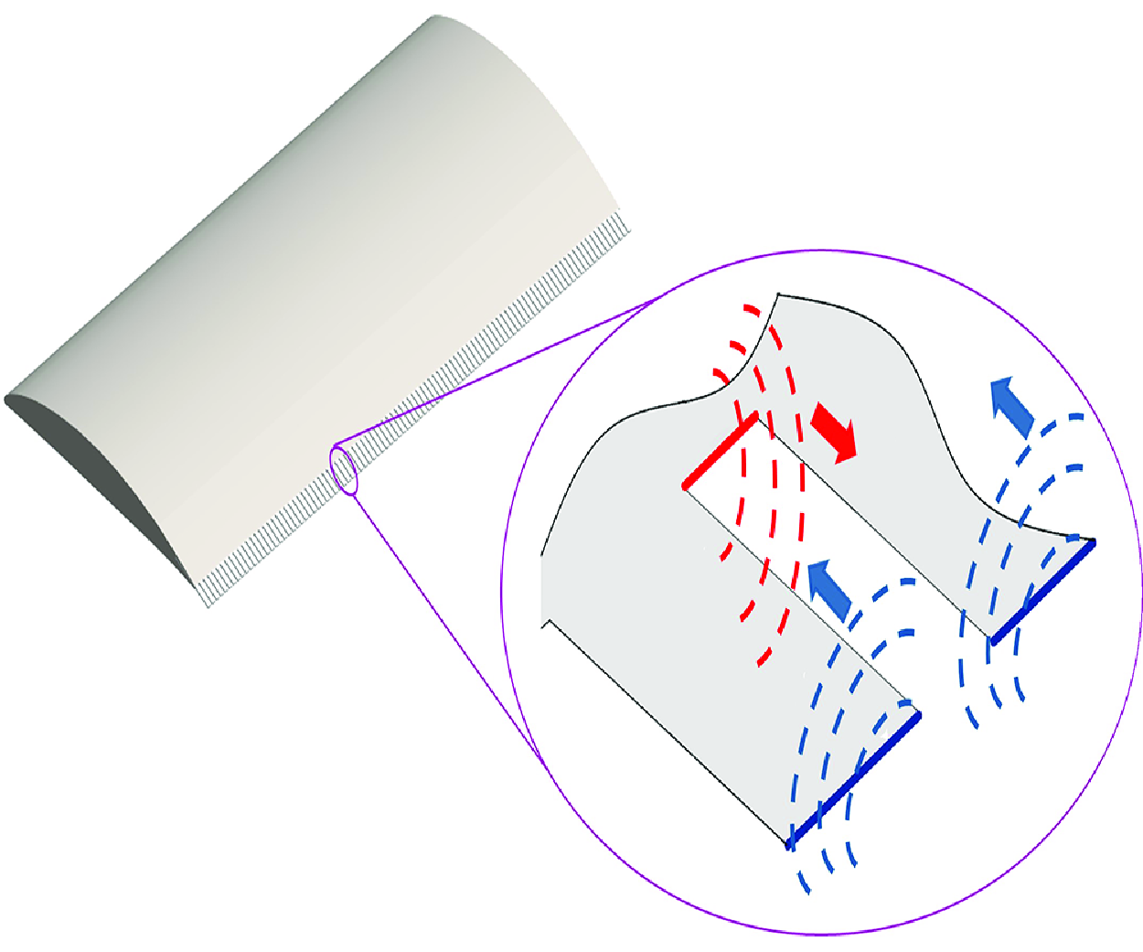
The underlying concept of trailing edge slits for the reduction of aerofoil trailing edge self-noise is the destructive interference between the two highly coherent compact sources at the root of the slit and at the tip, $S_{1}$
and
$S_{1}$
and $S_{2}$
, respectively, as depicted in figure 1. These localised sources are generated after interaction between the boundary layer and edge
$S_{2}$
, respectively, as depicted in figure 1. These localised sources are generated after interaction between the boundary layer and edge $S_{1}$
, as well as the two edges at
$S_{1}$
, as well as the two edges at $S_{2}$
. As a result they are highly coherent since they are generated by the same turbulent eddies in the boundary layer but delayed in time by
$S_{2}$
. As a result they are highly coherent since they are generated by the same turbulent eddies in the boundary layer but delayed in time by $H/U_c$
, where H is the length of the slit as shown in figure 1, which corresponds to the streamwise separation distance between the two sources, and
$H/U_c$
, where H is the length of the slit as shown in figure 1, which corresponds to the streamwise separation distance between the two sources, and $U_c$
is the turbulent eddies convection speed. The important parameter determining the frequency of maximum noise reduction is therefore the non-dimensional Strouhal frequency
$U_c$
is the turbulent eddies convection speed. The important parameter determining the frequency of maximum noise reduction is therefore the non-dimensional Strouhal frequency $St$
, which is defined as
$St$
, which is defined as
 \begin{equation} St = \frac {f H}{U_c}, \end{equation}
where f is the frequency in dimensional form. The non-dimensional quantity $St$
corresponds to the ratio of the slit length
$St$
corresponds to the ratio of the slit length $H$
to the hydrodynamic wavelength
$H$
to the hydrodynamic wavelength $U_c/f$
. We note that
$U_c/f$
. We note that $2\pi St$
corresponds to the phase difference at frequency
$2\pi St$
corresponds to the phase difference at frequency $\omega$
between the two sources at either ends of the slit. Maximum destructive interference, and hence maximum noise reduction, are therefore predicted to occur at the discrete frequencies
$\omega$
between the two sources at either ends of the slit. Maximum destructive interference, and hence maximum noise reduction, are therefore predicted to occur at the discrete frequencies $St_n$
, given by
$St_n$
, given by
 \begin{equation} St_n= \frac {n}{2} \end{equation}
when $n$
is any odd natural number 1, 3, 5, etc.
$n$
is any odd natural number 1, 3, 5, etc.
By contrast, perfect constructive interference occurs when the acoustic radiation between the two sources are in-phase. This is therefore predicted to occur at the discrete frequencies $St_n$
in (2.2) when
$St_n$
in (2.2) when $n$
is any even natural number 2, 4, 6, etc.
$n$
is any even natural number 2, 4, 6, etc.
Assuming the validity of the noise principle described above, the use of trailing edge slits therefore allows, for the first time, maximum noise reductions to be targeted at a desired frequency range by the appropriate choice of slit length $H$
for a particular flow speed, according to (2.1) and (2.2).
$H$
for a particular flow speed, according to (2.1) and (2.2).
3. Research methodologies
3.1. Design of the slit trailing edges
This section describes the design of the slit trailing edge geometry. In this study, a NACA 65(12)−10 aerofoil with a span of 0.3 m is investigated experimentally. A 0.8 mm slot along the rear end of the aerofoil was manufactured to allow the insertion of various detachable, laser-cut flat plates of 0.8 mm thickness. A straight trailing edge is served as the baseline, while different slit geometries were cut into the flat plate to investigate the effect on noise radiation due to the slitted trailing edges. The overall chord length of the aerofoil varies between $c_\circ$
= 0.1425 m and 0.170 m depending on the slit length
$c_\circ$
= 0.1425 m and 0.170 m depending on the slit length $H$
. Coarse sandpaper strips of 10 mm width and an average roughness height of 0.95 mm were applied to the upper and lower surfaces of the aerofoil at
$H$
. Coarse sandpaper strips of 10 mm width and an average roughness height of 0.95 mm were applied to the upper and lower surfaces of the aerofoil at $x/\overline {c_\circ }=0.2$
, with
$x/\overline {c_\circ }=0.2$
, with $x=0$
refers to the aerofoil leading edge, to ensure that the boundary layers near the trailing edge are fully turbulent. Note that
$x=0$
refers to the aerofoil leading edge, to ensure that the boundary layers near the trailing edge are fully turbulent. Note that $\overline {c_\circ }$
is the aerofoil chord not counting the slit add-on. The aerofoil’s geometrical angle of attack is maintained at zero throughout the experiment. Validation through comparison of the measured surface pressure coefficients with the flow simulation, conducted under the same open jet configuration as the experiment to ensure consistent flow conditions, confirms that the effective angle of attack is also close to zero (Woodhead Reference Woodhead2021).
$\overline {c_\circ }$
is the aerofoil chord not counting the slit add-on. The aerofoil’s geometrical angle of attack is maintained at zero throughout the experiment. Validation through comparison of the measured surface pressure coefficients with the flow simulation, conducted under the same open jet configuration as the experiment to ensure consistent flow conditions, confirms that the effective angle of attack is also close to zero (Woodhead Reference Woodhead2021).
Apart from the length H, the slit geometry is also defined by its wavelength $\lambda$
, as shown in figure 1. The width of the slit root (back edge) is defined as W, and the width of the front edge is defined as a, resulting in
$\lambda$
, as shown in figure 1. The width of the slit root (back edge) is defined as W, and the width of the front edge is defined as a, resulting in $\lambda = W + a$
. The slit length H and wavelength
$\lambda = W + a$
. The slit length H and wavelength $\lambda$
were varied in the ranges of 5 mm
$\lambda$
were varied in the ranges of 5 mm $\leq$
H
$\leq$
H $\leq$
30 mm (interval of every 5 mm), and 3 mm
$\leq$
30 mm (interval of every 5 mm), and 3 mm $\leq \lambda$ $\leq$
35 mm. Additional geometrical definitions include 0.15 mm
$\leq$
35 mm. Additional geometrical definitions include 0.15 mm $\leq$
a
$\leq$
a $\leq$
1.5 mm, and 1.5 mm
$\leq$
1.5 mm, and 1.5 mm $\leq$
W
$\leq$
W $\leq$
29.85 mm.
$\leq$
29.85 mm.
The baseline (non-slitted) trailing edge insert was chosen to be half the length of the slitted insert to ensure that the wetted area is roughly the same. We note that, as far as the baseline aerofoil is concerned, the difference in the radiated trailing edge noise between $H/2=2.5$
mm and 15 mm is insignificant across the frequency range of interest.
$H/2=2.5$
mm and 15 mm is insignificant across the frequency range of interest.
3.2. Experimental set-up and data analysis
3.2.1. Noise measurements
The far-field noise and near-field boundary layer measurements were conducted in the aeroacoustics wind tunnel facility at Brunel University of London, UK. The wind tunnel is situated in a 4 m $\times$
5 m
$\times$
5 m $\times$
3.4 m anechoic chamber. The nozzle exit is rectangular with dimensions of 0.10 m (height)
$\times$
3.4 m anechoic chamber. The nozzle exit is rectangular with dimensions of 0.10 m (height) $\times$
0.30 m (width). This wind tunnel has a turbulence intensity of between 0.1%–0.2 % and a maximum jet velocity of approximately 80
$\times$
0.30 m (width). This wind tunnel has a turbulence intensity of between 0.1%–0.2 % and a maximum jet velocity of approximately 80 $\textrm {m s}^{-1}$
. The frequency range of interest for this study is between 0.2 and 20 kHz, with the lower limit determined by the cutoff frequency of the anechoic chamber. Within this frequency range, noise produced by the baseline aerofoil exceeds the background noise of the wind tunnel (with the side plates installed but without the aerofoil) by at least 10 dB (Vathylakis et al. Reference Vathylakis, Chaitanya, Chong and Joseph2016; Woodhead et al. Reference Woodhead, Chong, Joseph and Vathylakis2021). Additionally, a signal-to-noise ratio greater than 3 dB for the quietest slitted aerofoil is maintained across the above frequency range.
$\textrm {m s}^{-1}$
. The frequency range of interest for this study is between 0.2 and 20 kHz, with the lower limit determined by the cutoff frequency of the anechoic chamber. Within this frequency range, noise produced by the baseline aerofoil exceeds the background noise of the wind tunnel (with the side plates installed but without the aerofoil) by at least 10 dB (Vathylakis et al. Reference Vathylakis, Chaitanya, Chong and Joseph2016; Woodhead et al. Reference Woodhead, Chong, Joseph and Vathylakis2021). Additionally, a signal-to-noise ratio greater than 3 dB for the quietest slitted aerofoil is maintained across the above frequency range.
A polar array of microphones with a radius of 0.97 m comprising eight ${1}/{2}$
inch G.R.A.S. 46AE condenser microphones were used to measure the noise directivity and sound power level (PWL) from the aerofoil. The microphones were positioned at
${1}/{2}$
inch G.R.A.S. 46AE condenser microphones were used to measure the noise directivity and sound power level (PWL) from the aerofoil. The microphones were positioned at $50^\circ \leq \theta \leq 120^\circ$
with the microphone at
$50^\circ \leq \theta \leq 120^\circ$
with the microphone at $\theta = 90^\circ$
being positioned directly above the trailing edge. The microphone signals were acquired at a sampling frequency of 40 kHz for a duration of 20 s using a 16-bit analogue–digital card from National Instruments. The PSD was computed from the sampled data, with a 1024-point Hanning window and a 50 % overlap, which provides a frequency resolution of 39 Hz. Noise measurements were made at free stream velocities between
$\theta = 90^\circ$
being positioned directly above the trailing edge. The microphone signals were acquired at a sampling frequency of 40 kHz for a duration of 20 s using a 16-bit analogue–digital card from National Instruments. The PSD was computed from the sampled data, with a 1024-point Hanning window and a 50 % overlap, which provides a frequency resolution of 39 Hz. Noise measurements were made at free stream velocities between $U_\infty$
= 20 and 60
$U_\infty$
= 20 and 60 $\textrm {m s}^{-1}$
. The sound power spectra, per unit span, were calculated by assuming cylindrical spreading of the noise from the trailing edge, according to
$\textrm {m s}^{-1}$
. The sound power spectra, per unit span, were calculated by assuming cylindrical spreading of the noise from the trailing edge, according to
 \begin{equation} \mathcal{W}(f) = \frac {2 \pi r \sum \limits _{i=1}^{N} S_{pp}(f,\theta _i) \Delta \theta }{\rho c_\infty },\quad N = 8 \end{equation}
where $c_\infty$
is the speed of sound,
$c_\infty$
is the speed of sound, $\rho$
is the air density,
$\rho$
is the air density, $S_{pp}$
is the far-field pressure power spectrum density at a polar angle
$S_{pp}$
is the far-field pressure power spectrum density at a polar angle $\theta$
over the range of angles,
$\theta$
over the range of angles, $50^\circ (\theta _1) \leq \theta \leq 120^\circ (\theta _8)$
and
$50^\circ (\theta _1) \leq \theta \leq 120^\circ (\theta _8)$
and $\Delta \theta = 10^\circ$
is the angle between adjacent microphones. The sound power
$\Delta \theta = 10^\circ$
is the angle between adjacent microphones. The sound power $\mathcal{W}(f)$
was deduced by integrating the mean square pressure over the microphone array. Against a reference
$\mathcal{W}(f)$
was deduced by integrating the mean square pressure over the microphone array. Against a reference $\mathcal{W}_0 = 10^{-12}$
W, the sound PWL spectrum can be calculated from
$\mathcal{W}_0 = 10^{-12}$
W, the sound PWL spectrum can be calculated from
 \begin{equation} {PWL}(f) = 10\log _{10} \left [\frac {\mathcal{W}(f)}{\mathcal{W}_0}\right ]. \end{equation}
3.2.2. Unsteady velocity measurements
In the investigation of the flow field, unsteady velocity measurements were conducted by hot wire anemometry at $U_\infty = 30$ $\textrm {m s}^{-1}$
, corresponding to a Reynolds number of 3.1
$\textrm {m s}^{-1}$
, corresponding to a Reynolds number of 3.1 $\times$ $10^{5}$
. The hot wire probes are the DANTEC 55P11 straight miniature type, which is 5
$10^{5}$
. The hot wire probes are the DANTEC 55P11 straight miniature type, which is 5 $\unicode{x03BC}$
m in diameter and 1.25 mm in length. They were used to measure the velocity fluctuations within the flow with an overheat ratio set at 1.8 to achieve good velocity sensitivity. The velocity signals were digitised by a 16-bit analogue–digital converter at a sampling frequency of 20 kHz. The hot wire probes are mounted on a three-dimensional traverse system with a resolution of 0.01 mm in all directions.
$\unicode{x03BC}$
m in diameter and 1.25 mm in length. They were used to measure the velocity fluctuations within the flow with an overheat ratio set at 1.8 to achieve good velocity sensitivity. The velocity signals were digitised by a 16-bit analogue–digital converter at a sampling frequency of 20 kHz. The hot wire probes are mounted on a three-dimensional traverse system with a resolution of 0.01 mm in all directions.
The postanalysis of the unsteady streamwise velocity focuses on the PSD, coherence and cross-correlation pertinent to the change in the turbulent boundary layer structure by the slitted geometry. The coherence examines the ‘similarity’ between two points in the frequency domain, which is defined as
 \begin{equation} \gamma _k^2(f) = \frac {|\Phi _{v_iv_j}(f)|^2}{\Phi _{v_iv_i}(f) \Phi _{v_jv_j}(f)}, \quad k=x,z \end{equation}
where $\Phi _{v_iv_j}(f)$
is the cross-PSD of velocity fluctuations measured by a stationary hot wire probe i and a traversing hot wire probe j. Here
$\Phi _{v_iv_j}(f)$
is the cross-PSD of velocity fluctuations measured by a stationary hot wire probe i and a traversing hot wire probe j. Here $\Phi _{v_iv_i} (f)$
and
$\Phi _{v_iv_i} (f)$
and $\Phi _{v_jv_j} (f)$
are the auto-PSD of the stationary and non-stationary velocity fluctuations, respectively. The index k = x and z is to differentiate the coherence in the streamwise and spanwise directions, respectively. The cross-correlation examines the time lag of two signals, which is defined as
$\Phi _{v_jv_j} (f)$
are the auto-PSD of the stationary and non-stationary velocity fluctuations, respectively. The index k = x and z is to differentiate the coherence in the streamwise and spanwise directions, respectively. The cross-correlation examines the time lag of two signals, which is defined as
 \begin{equation} R_{ij}(\tau ) = \frac {\overline {v_i^\prime (x_i,t)v_j^\prime (x_j,t-\tau )}}{v_{i\,prms}^\prime (x_i)v_{j\,prms}^\prime (x_j)}, \end{equation}
where $v_i^\prime$
and
$v_i^\prime$
and $v_j^\prime$
are the velocity fluctuations measured from both hot wires situated at positions
$v_j^\prime$
are the velocity fluctuations measured from both hot wires situated at positions $x_i$
and
$x_i$
and $x_j$
, respectively. Here
$x_j$
, respectively. Here $\tau$
is the time delay between the signals, and
$\tau$
is the time delay between the signals, and $v_{i\,prms}^\prime$
and
$v_{i\,prms}^\prime$
and $v_{j\,prms}^\prime$
are the root-mean-square of the velocity fluctuations measured by hot wire i and j, respectively.
$v_{j\,prms}^\prime$
are the root-mean-square of the velocity fluctuations measured by hot wire i and j, respectively.
Spatial distribution and coordinate system for the slit’s root, mid and tip regions, respectively.

4. Measurements of steady and unsteady flow in the vicinity of the slit trailing edge
4.1. Measurement procedure
Boundary layer measurements were made at the slit root, midway along the slit and at the slit tip on both surfaces of the aerofoil. The same measurement locations were also chosen for the baseline trailing edge. These locations are identified by non-dimensionalised coordinates $x^\prime$
and
$x^\prime$
and $z^\prime$
, as illustrated in figure 2.
$z^\prime$
, as illustrated in figure 2.
The slit trailing edge investigated in the flow measurements contains the following configurations: H = 15 mm and $\lambda$
= 3 mm. The inflow velocity is set at
$\lambda$
= 3 mm. The inflow velocity is set at $U_\infty$
= 30
$U_\infty$
= 30 $\textrm {m s}^{-1}$
. Measurements were made of the mean and fluctuating velocity boundary layer profiles at several locations near the trailing edge, on both the suction and pressure surfaces of the aerofoil. The measurements were made in the
$\textrm {m s}^{-1}$
. Measurements were made of the mean and fluctuating velocity boundary layer profiles at several locations near the trailing edge, on both the suction and pressure surfaces of the aerofoil. The measurements were made in the $x{-}y$
plane with the hot wire kept parallel to the wall surface. The hot wire was traversed in steps of 0.1 mm from the wall surface in order to capture the large velocity gradients in the near wall region. A distance of 0.1 mm from the wall corresponds to
$x{-}y$
plane with the hot wire kept parallel to the wall surface. The hot wire was traversed in steps of 0.1 mm from the wall surface in order to capture the large velocity gradients in the near wall region. A distance of 0.1 mm from the wall corresponds to $y^+ = 6.7$
for the turbulent boundary layer developed on the suction surface trailing edge, where
$y^+ = 6.7$
for the turbulent boundary layer developed on the suction surface trailing edge, where $y^+ = y u_\tau /\nu$
(y is the vertical distance from the wall,
$y^+ = y u_\tau /\nu$
(y is the vertical distance from the wall, $u_\tau$
is the friction velocity and
$u_\tau$
is the friction velocity and $\nu$
is the kinematic viscosity of air).
$\nu$
is the kinematic viscosity of air).
The hot wire signals were also used to measure the streamwise coherence ( $\gamma _x$
) and cross-correlation of the unsteady velocity between the slit’s root and tip. The hot wire probes were reorientated such that the wires are perpendicular to the wall surface. The midpoint of the wire was located at approximately 0.73 mm from the wall surface, corresponding to
$\gamma _x$
) and cross-correlation of the unsteady velocity between the slit’s root and tip. The hot wire probes were reorientated such that the wires are perpendicular to the wall surface. The midpoint of the wire was located at approximately 0.73 mm from the wall surface, corresponding to $y^+ = 49$
. The streamwise coherence and cross-correlation measurements were measured between two hot wire probes. One is situated at the reference stationary point, which is at the centre of the slit root gap region (
$y^+ = 49$
. The streamwise coherence and cross-correlation measurements were measured between two hot wire probes. One is situated at the reference stationary point, which is at the centre of the slit root gap region ( $x^\prime ,\, z^\prime$
) = (0, 0.5), while the other probe is traversed from a position just 0.5 mm behind the stationary probe to the tip (
$x^\prime ,\, z^\prime$
) = (0, 0.5), while the other probe is traversed from a position just 0.5 mm behind the stationary probe to the tip ( $x^\prime ,\, z^\prime$
) = (1.0, 0.5) of the slit trailing edge. The streamwise separation distance between the two hot wire probes, in dimensional form, is hitherto represented by
$x^\prime ,\, z^\prime$
) = (1.0, 0.5) of the slit trailing edge. The streamwise separation distance between the two hot wire probes, in dimensional form, is hitherto represented by $\eta _x$
. Note that the two-point measurements are conducted on both the suction and pressure surfaces of the aerofoil. Identical hot wire positions were chosen to quantify the flow around the baseline trailing edge, which shares the same H as the slit trailing edge in all the flow measurements.
$\eta _x$
. Note that the two-point measurements are conducted on both the suction and pressure surfaces of the aerofoil. Identical hot wire positions were chosen to quantify the flow around the baseline trailing edge, which shares the same H as the slit trailing edge in all the flow measurements.
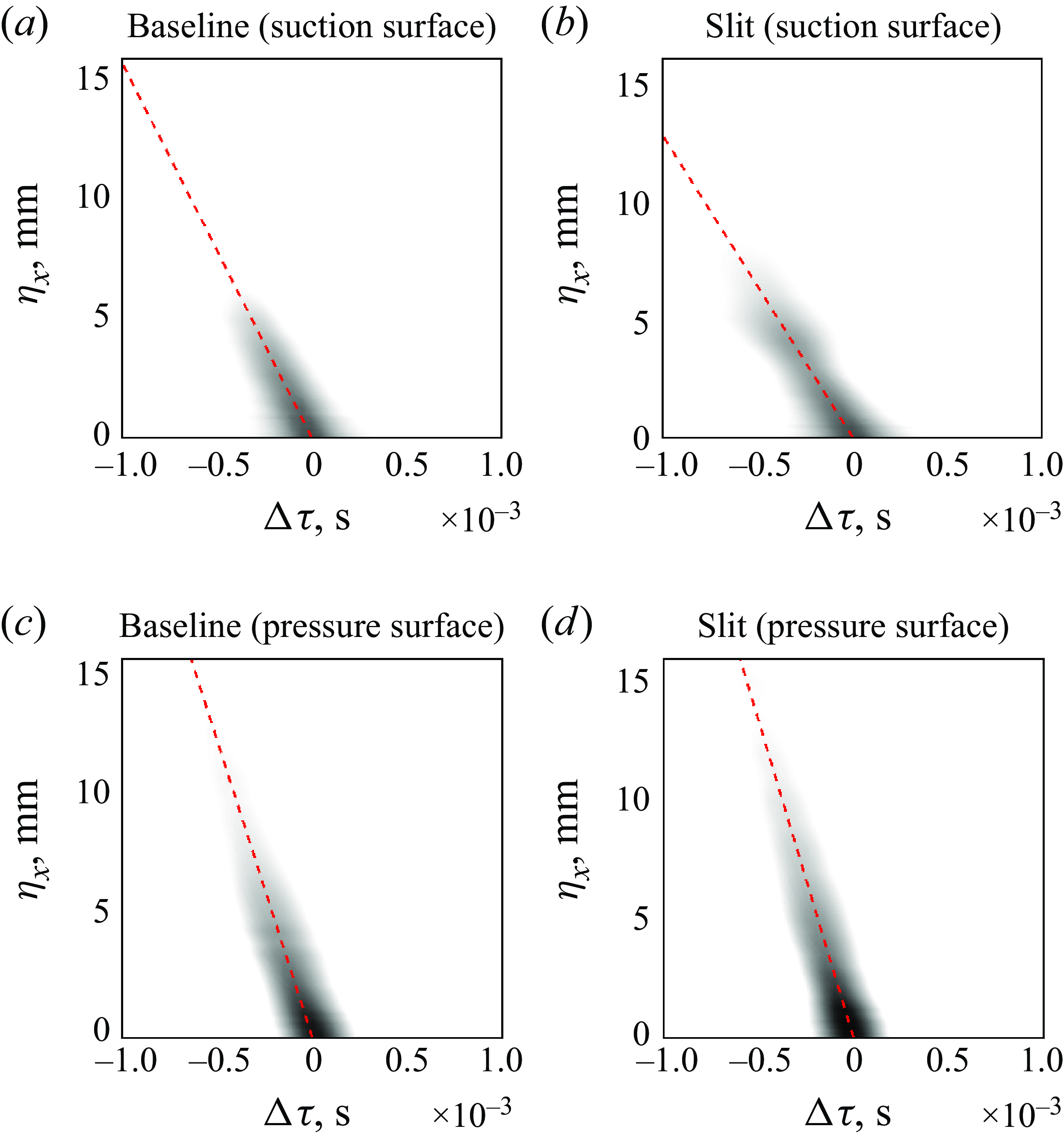
Comparison between the (a,c) baseline trailing edge and (b,d) slit trailing edge for their $\gamma _x$
where H = 15 mm, W = 0.3 mm and
$\gamma _x$
where H = 15 mm, W = 0.3 mm and $\lambda$
= 3 mm at
$\lambda$
= 3 mm at $U_\infty$
= 30
$U_\infty$
= 30 $\textrm {m s}^{-1}$
. The embedded line in all the contour plots is
$\textrm {m s}^{-1}$
. The embedded line in all the contour plots is $f = -\alpha . ({U_c \ln (\gamma _x)})/({2\pi b_1 \eta _x})$
.
$f = -\alpha . ({U_c \ln (\gamma _x)})/({2\pi b_1 \eta _x})$
.

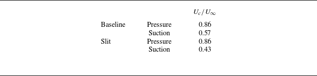
Results of the convection velocities of the turbulent eddies for the baseline and slit trailing edges on the pressure and suction surfaces.
4.2. Streamwise coherence $\gamma _x$
at the slit proximity
$\gamma _x$
at the slit proximity

Figure 3 shows a comparison of coherence contours $\gamma _x$
versus frequency and streamwise separation distance
$\gamma _x$
versus frequency and streamwise separation distance $\eta _x$
between the baseline and slit trailing edges at both the suction and pressure surfaces. In general, the coherence level is higher and spans a larger footprint in the
$\eta _x$
between the baseline and slit trailing edges at both the suction and pressure surfaces. In general, the coherence level is higher and spans a larger footprint in the $f- \eta _x$
domain on the pressure surface than on the suction surface (note the difference in colour map scaling between them). This is due to the eddies with larger integral length scale on the pressure surface where the turbulent boundary layer is several times thicker than that on the suction surface. Also shown in these figures is the curve
$f- \eta _x$
domain on the pressure surface than on the suction surface (note the difference in colour map scaling between them). This is due to the eddies with larger integral length scale on the pressure surface where the turbulent boundary layer is several times thicker than that on the suction surface. Also shown in these figures is the curve $f=-\alpha U_c \ln (\gamma _x) /2\pi b_1 \eta _x$
, obtained by solving for
$f=-\alpha U_c \ln (\gamma _x) /2\pi b_1 \eta _x$
, obtained by solving for $f$
using the Corcos model for streamwise coherence (Corcos Reference Corcos1962, Reference Corcos1963), where
$f$
using the Corcos model for streamwise coherence (Corcos Reference Corcos1962, Reference Corcos1963), where $b_1$
is an empirical decay factor in the streamwise direction. This function follows closely the contours of constant coherence once the constant
$b_1$
is an empirical decay factor in the streamwise direction. This function follows closely the contours of constant coherence once the constant $\alpha$
is chosen appropriately, thereby validating the applicability of the Corcos model in our investigation. Note that the
$\alpha$
is chosen appropriately, thereby validating the applicability of the Corcos model in our investigation. Note that the $U_c$
in the curves is obtained from table 1, which will be discussed in § 4.4.
$U_c$
in the curves is obtained from table 1, which will be discussed in § 4.4.
For the baseline aerofoil shown in figure 3, the coherence contours exhibit high levels in the low-to-mid frequency range, 100 Hz $\lt f \lt$
4 kHz, which we later designate as the acoustical-interference frequency zone, for both the suction and pressure surfaces as
$\lt f \lt$
4 kHz, which we later designate as the acoustical-interference frequency zone, for both the suction and pressure surfaces as $\eta _x \rightarrow 0$
. In contrast, negligible coherence is observed at higher frequencies, limiting the potential for destructive interference at these frequencies. The decay rate of the turbulent eddies at the pressure surface is similar to that on the suction surface. Near the trailing edge, at
$\eta _x \rightarrow 0$
. In contrast, negligible coherence is observed at higher frequencies, limiting the potential for destructive interference at these frequencies. The decay rate of the turbulent eddies at the pressure surface is similar to that on the suction surface. Near the trailing edge, at $\eta _x$
= 15 mm, coherence levels as high as 0.45 are achieved at
$\eta _x$
= 15 mm, coherence levels as high as 0.45 are achieved at $f \leq 700$
Hz. A significant portion of the coherence contours remains evident at larger streamwise separation distances, with non-negligible coherence level still observable for
$f \leq 700$
Hz. A significant portion of the coherence contours remains evident at larger streamwise separation distances, with non-negligible coherence level still observable for $\eta _x \gt$
15 mm.
$\eta _x \gt$
15 mm.
For the slit trailing edge, a somewhat different picture is observed at the suction surface. The decay of $\gamma _x$
can be observed to deviate from the Corcos model. The core level of
$\gamma _x$
can be observed to deviate from the Corcos model. The core level of $\gamma _x$
at
$\gamma _x$
at $\eta _x \lt 5$
mm is evidently shrunk in comparison with the baseline trailing edge. This illustrates that the turbulent eddy scales at close proximity to the slit root region deviates from the otherwise nominal turbulent boundary layer developed on a flat surface. Away from the root and towards the tip, an abrupt disappearance of the
$\eta _x \lt 5$
mm is evidently shrunk in comparison with the baseline trailing edge. This illustrates that the turbulent eddy scales at close proximity to the slit root region deviates from the otherwise nominal turbulent boundary layer developed on a flat surface. Away from the root and towards the tip, an abrupt disappearance of the $\gamma _x$
footprint at the entire frequency range is observed when
$\gamma _x$
footprint at the entire frequency range is observed when $\eta _x \gt 7.5$
mm, i.e. from the mid region of the slit (
$\eta _x \gt 7.5$
mm, i.e. from the mid region of the slit ( $x^\prime = 0.5$
) towards the tip (
$x^\prime = 0.5$
) towards the tip ( $x^\prime = 1.0$
).
$x^\prime = 1.0$
).
It is clear that the presence of the cross-flow through the slit trailing edge (from the pressure surface to the suction surface), and the ensuing formation of a pair of secondary flow structures in the form of counter-rotating streamwise vortices observed in Woodhead (Reference Woodhead2021), are responsible for the difference in the behaviour of $\gamma _x$
for the slit trailing edge at the suction surface.
$\gamma _x$
for the slit trailing edge at the suction surface.
The stationary and traversing hot wire probes used for the coherence measurement both have sensing lengths of approximately 1.25 mm. At the slit root region ( $x^\prime = 0$
), where the streamwise vortices are still relatively close to the suction wall surface (Woodhead Reference Woodhead2021), signals measured by the probes would be dominated by the dynamics of these streamwise vortices. This explains the change in the behaviour of
$x^\prime = 0$
), where the streamwise vortices are still relatively close to the suction wall surface (Woodhead Reference Woodhead2021), signals measured by the probes would be dominated by the dynamics of these streamwise vortices. This explains the change in the behaviour of $\gamma _x$
at small values of
$\gamma _x$
at small values of $\eta _x$
. As
$\eta _x$
. As $\eta _x$
(and
$\eta _x$
(and $x^\prime$
) is increased, these streamwise vortices will be lifted up during which eddies with high level of turbulent kinetic energy will be transported away from the wall surface (Woodhead Reference Woodhead2021). The detached turbulent shear layer will be outside the sensing element of both hot wire probes. This explains the rapid decay of
$x^\prime$
) is increased, these streamwise vortices will be lifted up during which eddies with high level of turbulent kinetic energy will be transported away from the wall surface (Woodhead Reference Woodhead2021). The detached turbulent shear layer will be outside the sensing element of both hot wire probes. This explains the rapid decay of $\gamma _x$
on the suction surface of the slit trailing edge. Once the flow reaches the slit tip the turbulent eddies are no longer close to the wall surface. This phenomenon might have some effects on the coherence-based acoustic scattering mechanism.
$\gamma _x$
on the suction surface of the slit trailing edge. Once the flow reaches the slit tip the turbulent eddies are no longer close to the wall surface. This phenomenon might have some effects on the coherence-based acoustic scattering mechanism.
The characteristics of $\gamma _x$
at the pressure surface of the slit trailing edge appear to be similar to those of the baseline counterpart. This suggests that the local turbulent boundary layer is not significantly affected by the slit on the pressure surface, a conclusion that will be confirmed by the boundary layer profiles in § 4.3. It is important to note that the maintenance of high coherence levels at
$\gamma _x$
at the pressure surface of the slit trailing edge appear to be similar to those of the baseline counterpart. This suggests that the local turbulent boundary layer is not significantly affected by the slit on the pressure surface, a conclusion that will be confirmed by the boundary layer profiles in § 4.3. It is important to note that the maintenance of high coherence levels at $x^\prime = 1.0$
at the pressure surface of the slit trailing edge indicates that the scattering of pressure waves at the slit root and tip, respectively, is likely to be coherent. As a result, the degree of acoustical interference is expected to be dominant.
$x^\prime = 1.0$
at the pressure surface of the slit trailing edge indicates that the scattering of pressure waves at the slit root and tip, respectively, is likely to be coherent. As a result, the degree of acoustical interference is expected to be dominant.
Comparison of the mean velocity profiles for the baseline and slit trailing edges at the root ( $x^\prime = 0$
), mid (
$x^\prime = 0$
), mid ( $x^\prime = 0.5$
) and tip (
$x^\prime = 0.5$
) and tip ( $x^\prime = 1.0$
) for the (a) suction surface and (b) pressure surface where H = 15 mm, W = 0.3 mm and
$x^\prime = 1.0$
) for the (a) suction surface and (b) pressure surface where H = 15 mm, W = 0.3 mm and $\lambda$
= 3 mm at
$\lambda$
= 3 mm at $U_\infty$
= 30
$U_\infty$
= 30 $\textrm {m s}^{-1}$
.
$\textrm {m s}^{-1}$
.

Comparison of the non-dimensional velocity fluctuation (turbulence intensity, I) for the baseline and slit trailing edges at the root ( $x^\prime = 0$
), mid (
$x^\prime = 0$
), mid ( $x^\prime = 0.5$
) and tip (
$x^\prime = 0.5$
) and tip ( $x^\prime = 1.0$
) for the (a) suction surface and (b) pressure surface where H = 15 mm, W = 0.3 mm and
$x^\prime = 1.0$
) for the (a) suction surface and (b) pressure surface where H = 15 mm, W = 0.3 mm and $\lambda$
= 3 mm at
$\lambda$
= 3 mm at $U_\infty$
= 30
$U_\infty$
= 30 $\textrm {m s}^{-1}$
.
$\textrm {m s}^{-1}$
.

4.3. Boundary layer characteristics at the slit root, mid and tip regions
We now investigate the effect by the slit on the mean velocity boundary layer profile. Figure 4 shows boundary layer profiles for the baseline and slit trailing edges at the root ( $x^\prime = 0$
), midway of the slit (
$x^\prime = 0$
), midway of the slit ( $x^\prime = 0.5$
) and at the tip (
$x^\prime = 0.5$
) and at the tip ( $x^\prime = 1.0$
). On the suction surface of the slit root region, the boundary layer profile appears slightly thicker than at the same location of the baseline aerofoil. However, at the mid and tip regions, inflection points in the boundary layer profile are present due to coalescence between the secondary flow structures from the cross-flow, and the local turbulent boundary layer.
$x^\prime = 1.0$
). On the suction surface of the slit root region, the boundary layer profile appears slightly thicker than at the same location of the baseline aerofoil. However, at the mid and tip regions, inflection points in the boundary layer profile are present due to coalescence between the secondary flow structures from the cross-flow, and the local turbulent boundary layer.
The flow dynamics can be further examined from the turbulence intensity profiles, shown in figure 5. Whilst the turbulence intensity is only marginally increased at the root location on the suction surface, at the mid and tip regions there is now a significant upward displacement of the turbulence maxima. In addition, the peak turbulence level also increases from 8 % (baseline) to 10 % (slit). In contrast, the effect of the slit on the pressure surface steady ( $\overline {U}/U_\infty$
) and unsteady (
$\overline {U}/U_\infty$
) and unsteady ( $U_{rms}/U_\infty$
) boundary layer profiles is much less affected.
$U_{rms}/U_\infty$
) boundary layer profiles is much less affected.
On the pressure surface, the boundary layer mean velocity profiles for both the baseline and slit trailing edges in figure 4 are significantly different in comparison with the suction surface. Although at a geometrical angle of attack of zero degree the pressure gradients experienced by both sides of the aerofoil are already markedly different due to the highly cambered configuration. The pressure surface turbulent boundary layer is several times thicker than that developed on the suction surface. At the root region, the near wall velocity excess shown in figure 4 for the slit trailing edge is notably greater than the baseline profile. This is due to the local acceleration of the leakage flow from the pressure surface to the suction surface through the slit. However, when leakage flow proceeds to the mid and tip regions for the slit trailing edge, the near wall velocity excess (in comparison with the baseline boundary layer profiles) becomes less significant. Examination of the turbulence intensity profiles in figure 5 shows that the near wall turbulence intensity level for the slit trailing edge at the mid and tip regions are similar to the baseline profiles. Therefore, the effects observed on the suction surface of the secondary flow structure are less evident on the pressure surface (e.g. no inflection point is observed throughout the flow field at the pressure surface of the slit trailing edge). The local flow dynamics should instead be regarded as the feeder for the secondary flow structures that are dominant at the suction surface.
Cross-correlation coefficients in the $\eta _x$
and
$\eta _x$
and $\Delta \tau$
domains for the (a,c) baseline trailing edge and (b,d) slit trailing edge for the suction and pressure surfaces where H = 15 mm, W = 0.3 mm and
$\Delta \tau$
domains for the (a,c) baseline trailing edge and (b,d) slit trailing edge for the suction and pressure surfaces where H = 15 mm, W = 0.3 mm and $\lambda$
= 3 mm at
$\lambda$
= 3 mm at $U_\infty$
= 30
$U_\infty$
= 30 $\textrm {m s}^{-1}$
.
$\textrm {m s}^{-1}$
.
4.4. Convection velocity of the turbulent eddies from the root to tip (baseline and slit trailing edges)
The simple expression of the characteristic Strouhal frequency pertaining to acoustic wave interference (2.1), described earlier in § 2, highlights the important role of the convection velocity of the turbulent eddies. In this section, we will investigate the typical time taken for the turbulent eddies to convect between the root and tip of the slit trailing edge. The same raw data used for the analysis of the streamwise coherence in § 4.2 was used to compute the time-domain cross-correlation coefficients between the stationary hot wire probe located at the root and a hot wire probe that was traversed along the slit length. The results are plotted in figure 6 for both the baseline and slit trailing edges, and for both the suction and pressure surfaces. Correlation coefficients below the arbitrary threshold of 0.9 were set to zero to aid clarity of presentation. A line of best-fit through the data was obtained whose gradient is simply relayed to the convection velocity through $U_c=\Delta \eta _x/\Delta \tau$
, where
$U_c=\Delta \eta _x/\Delta \tau$
, where $\Delta \tau$
is the time delay. A summary of the convection velocities as the fraction of the local free stream velocity
$\Delta \tau$
is the time delay. A summary of the convection velocities as the fraction of the local free stream velocity $U_\infty$
is provided in table 1.
$U_\infty$
is provided in table 1.
The table shows that the convection velocities of the turbulent eddies at the suction surface are generally lower than at the pressure surface. This phenomenon, which is applicable to both the baseline and slit trailing edges, is caused by the imposing adverse pressure gradients. Gostelow, Melwani & Walker (Reference Gostelow, Melwani and Walker1996) concluded that the convection velocity of a turbulent spot (which shares similar characteristics with eddies in a turbulent boundary layer) can be retarded by adverse pressure gradient. This is consistent with the measured surface pressure coefficients where the level of adverse pressure gradient near the aerofoil’s trailing edge suction surface is significantly larger than that at the pressure surface.
The presence of the slit can be observed to significantly slow the convection velocity $U_c/U_\infty$
from 0.57 (baseline) to 0.43 for the slitted geometry at the suction surface. This is caused by the dominant secondary flow structure at the slit suction surface. As discussed in §§ 4.2 and 4.3, the secondary flow structure is transported along the edge of the slit between the root and tip. The interaction between the secondary structures and the turbulent boundary layer and the rate at which they converge between the root and tip will be slower.
$U_c/U_\infty$
from 0.57 (baseline) to 0.43 for the slitted geometry at the suction surface. This is caused by the dominant secondary flow structure at the slit suction surface. As discussed in §§ 4.2 and 4.3, the secondary flow structure is transported along the edge of the slit between the root and tip. The interaction between the secondary structures and the turbulent boundary layer and the rate at which they converge between the root and tip will be slower.
In contrast, the pressure surface convection velocities for both the baseline and slit trailing edges remain the same at $U_c/U_\infty$
= 0.86.
$U_c/U_\infty$
= 0.86.
Contour maps of the $\Delta$
PWL in the
$\Delta$
PWL in the $f{-}H$
domains for the slit trailing edges at 20
$f{-}H$
domains for the slit trailing edges at 20 $\textrm {m s}^{-1}$ $\leq U_\infty \leq$
60
$\leq U_\infty \leq$
60 $\textrm {m s}^{-1}$
.
$\textrm {m s}^{-1}$
.

5. Far-field acoustic results
5.1. Effect on noise reductions due to slit length (H)
The slit length, $H$
, is the most critical parameter influencing the overall performance and frequency characteristics of noise reductions caused by trailing edge slits. This parameter determines the time delay between the sources at both ends of the slit. Figure 7 presents colour map contours of the noise reduction spectra as a function of H within the range under investigation. Results are shown at five flow speeds between
$H$
, is the most critical parameter influencing the overall performance and frequency characteristics of noise reductions caused by trailing edge slits. This parameter determines the time delay between the sources at both ends of the slit. Figure 7 presents colour map contours of the noise reduction spectra as a function of H within the range under investigation. Results are shown at five flow speeds between $U_\infty = 20$
and
$U_\infty = 20$
and $60$
$60$ $\textrm {m s}^{-1}$
.
$\textrm {m s}^{-1}$
.
Note that the quantity presented in the figure is the $\Delta$
PWL, which is defined as the difference in the sound PWL between the baseline trailing edge of
$\Delta$
PWL, which is defined as the difference in the sound PWL between the baseline trailing edge of ${1}/{2}H$
and slit trailing edge of H. Therefore, a positive value of
${1}/{2}H$
and slit trailing edge of H. Therefore, a positive value of $\Delta$
PWL denotes noise reduction achieved by the slit trailing edge, and the opposite is true for a negative value of
$\Delta$
PWL denotes noise reduction achieved by the slit trailing edge, and the opposite is true for a negative value of $\Delta$
PWL. Also shown in the contour maps are the curves
$\Delta$
PWL. Also shown in the contour maps are the curves $St_n= {n}/{2}$
denoting the frequencies of maximum acoustic interference, with
$St_n= {n}/{2}$
denoting the frequencies of maximum acoustic interference, with $n = 1, 3,$
etc. representing destructive interference and
$n = 1, 3,$
etc. representing destructive interference and $n = 2, 4,$
etc. representing constructive interference.
$n = 2, 4,$
etc. representing constructive interference.
Figure 7 shows clear ‘bands’ of alternating noise reduction and noise increase, which closely follow the predicted variations in (2.2) for odd and even values of $n$
, respectively. This figure therefore provides validation of the noise reduction principle outlined in § 2. Noise reductions in excess of 5 dB are observed at the peak frequencies
$n$
, respectively. This figure therefore provides validation of the noise reduction principle outlined in § 2. Noise reductions in excess of 5 dB are observed at the peak frequencies $St= 0.5\ \textrm {and}\ 1.5$
, while noise increases due to constructive interference (i.e.
$St= 0.5\ \textrm {and}\ 1.5$
, while noise increases due to constructive interference (i.e. $St= 1.0$
) appears to be limited to no more than approximately 3 dB.
$St= 1.0$
) appears to be limited to no more than approximately 3 dB.
Before conducting a detailed investigation into the effectiveness of trailing edge slits for reducing trailing edge noise, we first introduce a simple model to predict their noise reduction capabilities. This model also serves as a theoretical framework for understanding the behaviour of trailing edge slits.
5.2. Simple model of noise radiation from slitted trailing edge aerofoil
The mathematical models to be discussed in this section build upon the general principles for leading edge slits first introduced by Chaitanya & Joseph (Reference Chaitanya and Joseph2018), with two significant extensions tailored to turbulent boundary layer trailing edge noise. First, it accounts for the differences in propagation times between sound generated at the root and tip. Second, it incorporates the streamwise and spanwise coherence functions between the root and tip sources, both of which are critical factors in turbulent boundary layer dynamics.
Figure 7 provides confirmation of the general principle underlying the use of trailing edge slits for aerofoil noise reductions, confirming the presence of compact coherent source regions at either side of the slit that interfere to produce the bands of alternative noise reduction and noise increase. The incoming turbulent boundary layer flow will first interact with the root of the slit to produce a localised source at the slit root creating a localised pressure difference $\Delta p_r(\omega )$
at this location. The turbulent eddies continue to convect over the trailing edge surface with a convection velocity
$\Delta p_r(\omega )$
at this location. The turbulent eddies continue to convect over the trailing edge surface with a convection velocity $U_c$
towards the slit tip. After a time delay
$U_c$
towards the slit tip. After a time delay $H/U_c$
, the same turbulent eddies will then interact with the tip of the slit trailing edge to produce another localised source region at a distance H farther downstream, producing a local pressure difference
$H/U_c$
, the same turbulent eddies will then interact with the tip of the slit trailing edge to produce another localised source region at a distance H farther downstream, producing a local pressure difference $\Delta p_t(\omega )$
. Our principle assumption is that the source distributions are highly concentrated around the root and tip and may therefore be regarded as compact, as indicated in figure 1 as the
$\Delta p_t(\omega )$
. Our principle assumption is that the source distributions are highly concentrated around the root and tip and may therefore be regarded as compact, as indicated in figure 1 as the $\Delta p_r(\omega )$
(red line) and
$\Delta p_r(\omega )$
(red line) and $\Delta p_t(\omega )$
(blue lines), respectively.
$\Delta p_t(\omega )$
(blue lines), respectively.
The two compact source regions at the root $\zeta =0$
and tip
$\zeta =0$
and tip $\zeta =H$
can be represented by the Dirac delta functions,
$\zeta =H$
can be represented by the Dirac delta functions, $\Delta p_r (\omega ) \delta (\zeta )$
and
$\Delta p_r (\omega ) \delta (\zeta )$
and $\Delta p_t (\omega ) \delta (\zeta -H)$
, respectively. Substituting the sum of these distributions into the radiation integral due to Amiet (Reference Amiet1976) can produce the following expression for the far-field radiation across the slit with amplitude
$\Delta p_t (\omega ) \delta (\zeta -H)$
, respectively. Substituting the sum of these distributions into the radiation integral due to Amiet (Reference Amiet1976) can produce the following expression for the far-field radiation across the slit with amplitude $H$
:
$H$
:
 \begin{equation} \begin{aligned} p(x_1, x_2, \omega ) &\sim \displaystyle \frac {x_1}{4 \pi c_\infty \sigma } \int _0^H \left [ \Delta p_r(\omega )\delta (\zeta ) + \Delta p_t(\omega )\delta (\zeta - H) \right ] \\ &\quad \times \exp \left \{ -i \left [ \frac {\omega }{c_\infty \beta ^2} \left ( \frac {M - x_1}{\sigma } \right ) \zeta \right ] \right \} \, {\rm d}\zeta \end{aligned} \end{equation}
where $M$
is the Mach number, and
$M$
is the Mach number, and $\sigma$
is the flow-corrected distance,
$\sigma$
is the flow-corrected distance,
 \begin{equation} \sigma ^2 = x_1^2 + \beta ^2 x_2^2, \end{equation}
and
 \begin{equation} \beta ^2 = 1 - M^2. \end{equation}
In this analysis, we assume that adjacent slits are spaced farther apart than the turbulence length scale, ensuring that significant interference occurs only within the same slit. Consequently, adjacent slits will radiate noise incoherently. The PSD of the unsteady wall pressure for each slit can therefore be summed without accounting for phase differences. After integrating over the slit length H, the far-field radiation from the slit takes the following form:
 \begin{equation} p(x_1,x_2,\omega ) \sim \frac {x_1}{4 \pi c_\infty \sigma } \left [\Delta p_r (\omega ) +\Delta p_t (\omega )\right ] \exp \big[-i(\omega/(c_{\infty}\beta^{2})(M-x_1/\sigma)H\big]. \end{equation}
Consider the PSD of the far-field pressure radiation,
 \begin{equation} S_{pp}(x_1,x_2,\omega )=\frac {1}{T}E\left [p(x_1,x_2,\omega )p^*(x_1,x_2,\omega )\right ], \end{equation}
where $T$
is the time over which the Fourier transform is taken, which upon substitution of (5.4) yields
$T$
is the time over which the Fourier transform is taken, which upon substitution of (5.4) yields
 \begin{equation} \begin{aligned} S_{pp}(x_1,x_2,\omega ) &= \left ( \frac {x_1}{4 \pi c_\infty \sigma } \right )^2 \left \{ S_{\Delta p_{rr}}(\omega ) + S_{\Delta p_{tt}}(\omega )\vphantom{\frac {i \omega \left (M - \frac {x_1}{\sigma }\right ) H}{c_\infty \beta ^2}}\right. \\ &\quad + E \left [\Delta p_r(\omega )\Delta p_t^* (\omega )\right ] \exp \left [-\frac {i \omega \left (M - \frac {x_1}{\sigma }\right ) H}{c_\infty \beta ^2} \right ] \\ &\quad\left . + E \left [\Delta p_r^*(\omega )\Delta p_t (\omega )\right ] \exp \left [\frac {i \omega \left (M - \frac {x_1}{\sigma }\right ) H}{c_\infty \beta ^2} \right ] \right \}. \end{aligned} \end{equation}
The term $E[\Delta p_r^* (\omega ) \Delta p_t(\omega )]$
is the cross-PSD between the root and tip sources, which are separated by
$E[\Delta p_r^* (\omega ) \Delta p_t(\omega )]$
is the cross-PSD between the root and tip sources, which are separated by $H$
in the streamwise direction and by
$H$
in the streamwise direction and by $(w+a)/2$
in the spanwise direction, as illustrated in figure 1. This can be expressed in the following form:
$(w+a)/2$
in the spanwise direction, as illustrated in figure 1. This can be expressed in the following form:
 \begin{equation} \begin{aligned} \frac {1}{T} E\left [\Delta p_r^*(\omega ) \Delta p_t(\omega )\right ] &= \sqrt {S_{\Delta p_{rr}}(\omega ) S_{\Delta p_{tt}}(\omega )}\, \gamma _x \left [ \frac {H}{l_1(\omega )} \right ] \gamma _z \left [ \frac {w + a}{l_3(\omega )} \right ]\\&\quad \times \exp \left [ -\frac {i \omega H}{U_c(\omega )} \right ] \end{aligned} \end{equation}
where $\gamma _x [{H}/{l_1 (\omega )} ]$
is the boundary layer streamwise coherence function, which we assume to be only a function of the ratio of the streamwise separation distance H and the frequency-dependent coherence length scale
$\gamma _x [{H}/{l_1 (\omega )} ]$
is the boundary layer streamwise coherence function, which we assume to be only a function of the ratio of the streamwise separation distance H and the frequency-dependent coherence length scale $l_1 (\omega ) = ({U_c})/({\omega b_1})$
, where
$l_1 (\omega ) = ({U_c})/({\omega b_1})$
, where $b_1$
is a constant. On the other hand,
$b_1$
is a constant. On the other hand, $\gamma _z [({w+a})/({l_3 (\omega )}) ]$
is the coherence function in the spanwise direction. The phase of the cross spectrum
$\gamma _z [({w+a})/({l_3 (\omega )}) ]$
is the coherence function in the spanwise direction. The phase of the cross spectrum $({\omega H})/({U_c (\omega )})$
is assumed to be solely the time taken for the turbulent eddies to convect over the slit length H, where
$({\omega H})/({U_c (\omega )})$
is assumed to be solely the time taken for the turbulent eddies to convect over the slit length H, where $U_c (\omega )$
is the frequency-dependent convection velocity.
$U_c (\omega )$
is the frequency-dependent convection velocity.
The far-field radiated pressure PSD due to the slit can thus be expressed in the simpler form,
 \begin{equation} \begin{aligned} S_{pp}(x_1, x_2, \omega ) &= \left ( \frac {x_1}{4 \pi c_\infty \sigma } \right )^2 \left [ S_{\Delta p_{rr}}(\omega ) + S_{\Delta p_{tt}}(\omega ) \right ] \\ &\quad + 2 \sqrt {S_{\Delta p_{rr}}(\omega ) S_{\Delta p_{tt}}(\omega )}\, \gamma _x\left [ \frac {H}{l_1(\omega )} \right ] \gamma _z\left [ \frac {w + a}{l_3(\omega )} \right ] \cos \left [ \omega (\tau _H + \tau _A) \right ], \end{aligned} \end{equation}
where $\tau _H$
is the time taken for the turbulent eddies to convect along the slit length
$\tau _H$
is the time taken for the turbulent eddies to convect along the slit length $H$
,
$H$
,
 \begin{equation} \tau _H = \frac {H}{U_c (\omega )} \end{equation}
and $\tau _A$
represents the difference in propagation times to the observer between sound radiation from the root and from the tip of the slit. This difference can be expressed in terms of the observer angle
$\tau _A$
represents the difference in propagation times to the observer between sound radiation from the root and from the tip of the slit. This difference can be expressed in terms of the observer angle $\theta$
, where
$\theta$
, where $x_1=r\, \cos (\theta )$
and
$x_1=r\, \cos (\theta )$
and $ x_2=r\, \sin (\theta )$
, as follows:
$ x_2=r\, \sin (\theta )$
, as follows:
 \begin{equation} \tau _A (\theta ) = \frac {H}{c_\infty \beta ^2 } \left [\frac {M-\cos \theta }{\sqrt {\left (\cos ^2\theta +\beta ^2 \sin ^2\theta \right )}}\right ]. \end{equation}
Finally, to complete the simple analytical model for the radiation from the slit trailing edge, we adopt the forms of the streamwise and spanwise coherence functions for turbulent boundary layers as proposed by Corcos (Reference Corcos1962, Reference Corcos1963):
 \begin{align}& \gamma _x(\omega ,\eta _x) = \exp {\left (-b_1 \frac {\omega \eta _x}{U_c}\right )}, \end{align}
 \begin{align}& \gamma _z(\omega ,\eta _z) = \exp {\left (-b_3 \frac {\omega \eta _z}{U_c}\right )}, \end{align}
Comparison of the Corcos empirical model for the coherence in the streamwise direction to the experimental streamwise coherence $\gamma _x$
.
$\gamma _x$
.

where $b_1$
and
$b_1$
and $b_3$
are empirical decay factors in the streamwise and spanwise directions, respectively. This form of the coherence may be used to deduce the streamwise and spanwise coherence lengths defined in (5.11) and (5.12). Inspection of the above equations suggests that maximum reductions are obtained at the combination of angles
$b_3$
are empirical decay factors in the streamwise and spanwise directions, respectively. This form of the coherence may be used to deduce the streamwise and spanwise coherence lengths defined in (5.11) and (5.12). Inspection of the above equations suggests that maximum reductions are obtained at the combination of angles $\theta _n$
and frequencies
$\theta _n$
and frequencies $\omega _n$
, which satisfy
$\omega _n$
, which satisfy
 \begin{equation} \cos \left [ \omega _n \left ( \tau _H + \tau _A(\theta _n) \right ) \right ] = (2n - 1)\pi . \end{equation}
The use of the Corcos coherence function to predict noise reduction due to trailing edge slits will be validated next. Figure 8 compares the measured variation of $\gamma _x$
with the non-dimensional frequency
$\gamma _x$
with the non-dimensional frequency $\omega \eta _x/U_c$
, where
$\omega \eta _x/U_c$
, where $\eta _x$
= 1.8 mm at the pressure surface, against the theoretical form of (5.11) using an empirical decay constant
$\eta _x$
= 1.8 mm at the pressure surface, against the theoretical form of (5.11) using an empirical decay constant $b_1$
= 0.4. The results show good agreement with the experimental data.
$b_1$
= 0.4. The results show good agreement with the experimental data.
Comparison of the $\Delta$
SPL between the experimental and predicted results when H = (a) 10 mm, (b) 20 mm and (c) 30 mm of the slit trailing edge at
$\Delta$
SPL between the experimental and predicted results when H = (a) 10 mm, (b) 20 mm and (c) 30 mm of the slit trailing edge at $U_\infty$
= 40
$U_\infty$
= 40 $\textrm {m s}^{-1}$
.
$\textrm {m s}^{-1}$
.
5.3. Comparison between the experimental and predicted noise performance by slit trailing edges
Figure 9 shows a comparison of the measured and predicted sound pressure level (SPL) reduction $\Delta$
SPL versus
$\Delta$
SPL versus $St$
at the polar angle of
$St$
at the polar angle of $\theta = 90^\circ$
and flow speed of
$\theta = 90^\circ$
and flow speed of $U_\infty$
= 40
$U_\infty$
= 40 $\textrm {m s}^{-1}$
for the three slit lengths of
$\textrm {m s}^{-1}$
for the three slit lengths of $H=$
10, 20 and 30 mm, all of which contain
$H=$
10, 20 and 30 mm, all of which contain $\lambda$
= 3 mm and
$\lambda$
= 3 mm and $W$
= 0.3 mm. In most cases the variation of
$W$
= 0.3 mm. In most cases the variation of $\Delta$
SPL around the frequencies of maximum constructive interference (
$\Delta$
SPL around the frequencies of maximum constructive interference ( $S_t=$
1.0) and destructive interference (
$S_t=$
1.0) and destructive interference ( $S_t=$
0.5 and 1.5) are well captured by the theoretical expression of (2.2). Note that in the current prediction framework the source strengths at the root and tip are assumed to be equal,
$S_t=$
0.5 and 1.5) are well captured by the theoretical expression of (2.2). Note that in the current prediction framework the source strengths at the root and tip are assumed to be equal, $\Delta p_r(\omega )=\Delta p_t(\omega )$
, so that any loss in coherence between them arises solely from their streamwise and spanwise separation distances, and adjusted to give best fit to the measured noise reduction spectra. Note also that since the trailing edge source strength for the baseline aerofoil is unknown in relation to
$\Delta p_r(\omega )=\Delta p_t(\omega )$
, so that any loss in coherence between them arises solely from their streamwise and spanwise separation distances, and adjusted to give best fit to the measured noise reduction spectra. Note also that since the trailing edge source strength for the baseline aerofoil is unknown in relation to $\Delta p_r(\omega )$
and
$\Delta p_r(\omega )$
and $\Delta p_t(\omega )$
, it was chosen to provide best fit to the measured noise reduction spectra. Consequently, in this comparison we are limited to validating the accuracy of the model in predicting the shape of the noise reduction spectra and not its absolute level.
$\Delta p_t(\omega )$
, it was chosen to provide best fit to the measured noise reduction spectra. Consequently, in this comparison we are limited to validating the accuracy of the model in predicting the shape of the noise reduction spectra and not its absolute level.
The analytical model described by (5.8) shows satisfactory agreement with the measured SPL noise reduction, except at very low and very high frequencies. At very low frequencies, the measured noise reduction spectrum approaches 0 dB due to jet noise, which masks the radiated noise from the aerofoil. At very high frequencies, noise increases are observed, attributed to contributions from cross-flow within the slit gaps that are not accounted for in the analytical model. As a result, the continuous basis of acoustical interference assumed by the noise model is no longer consistent with the experimental observations at $St \gt 2$
.
$St \gt 2$
.
Overall, the predicted $\Delta \textrm {SPL}(S_t)$
provides a reasonable match to the experimental results at the primary frequencies. It is worth noting that the analytical model assumes that adjacent slits radiate incoherently, meaning interference occurs only between the root and tip of a single slit. In practice, however, there may be some interaction between adjacent slits due to partial coherence. This may be one of the causes of slight deviation between the measured and predicted sound reduction spectra observed here. While this effect may be readily incorporated into the model, it is likely to be a relatively weak contribution to the radiation spectra, as evidenced by the already strong agreement observed between measurements and predictions.
$\Delta \textrm {SPL}(S_t)$
provides a reasonable match to the experimental results at the primary frequencies. It is worth noting that the analytical model assumes that adjacent slits radiate incoherently, meaning interference occurs only between the root and tip of a single slit. In practice, however, there may be some interaction between adjacent slits due to partial coherence. This may be one of the causes of slight deviation between the measured and predicted sound reduction spectra observed here. While this effect may be readily incorporated into the model, it is likely to be a relatively weak contribution to the radiation spectra, as evidenced by the already strong agreement observed between measurements and predictions.
Comparison of the $\Delta$
SPL between the experimental and predicted results at
$\Delta$
SPL between the experimental and predicted results at $U_\infty$
= (a) 30
$U_\infty$
= (a) 30 $\textrm {m s}^{-1}$
and (b) 60
$\textrm {m s}^{-1}$
and (b) 60 $\textrm {m s}^{-1}$
when H = 20 mm for the slit trailing edge.
$\textrm {m s}^{-1}$
when H = 20 mm for the slit trailing edge.

We now investigate the effect of inflow velocity $U_\infty$
on the noise reduction spectra. Figure 10 shows a comparison between
$U_\infty$
on the noise reduction spectra. Figure 10 shows a comparison between $\Delta$
SPL achieved by the slit trailing edge for H = 20 mm,
$\Delta$
SPL achieved by the slit trailing edge for H = 20 mm, $\lambda$
= 3 mm and W = 0.3 mm, at two different inflow velocities of
$\lambda$
= 3 mm and W = 0.3 mm, at two different inflow velocities of $U_\infty$
= 30 and 60
$U_\infty$
= 30 and 60 $\textrm {m s}^{-1}$
. Acceptable qualitative agreement between the measured and predicted noise reduction can be observed at both inflow velocities. However, the most noteworthy aspect of these results is that noise reduction performance appears to improve with increasing flow speed, a phenomenon even more pronounced in figure 11. This behaviour contrasts with many noise reduction technologies, where control performance typically degrades as flow speed increases.
$\textrm {m s}^{-1}$
. Acceptable qualitative agreement between the measured and predicted noise reduction can be observed at both inflow velocities. However, the most noteworthy aspect of these results is that noise reduction performance appears to improve with increasing flow speed, a phenomenon even more pronounced in figure 11. This behaviour contrasts with many noise reduction technologies, where control performance typically degrades as flow speed increases.
The reason of this behaviour is readily explained by the form of the coherence functions in (5.11) which is a decaying function of $\omega \eta _x/U_c$
. Streamwise coherence is therefore predicted to increase as the convection speed
$\omega \eta _x/U_c$
. Streamwise coherence is therefore predicted to increase as the convection speed $U_c$
is increased, implying that the sources at the ends of the slit can interfere more effectively with increasing flow speed.
$U_c$
is increased, implying that the sources at the ends of the slit can interfere more effectively with increasing flow speed.
Another noteworthy aspect in figure 10 is the appearance of extra noise reduction peaks at $U_\infty$
= 60
$U_\infty$
= 60 $\textrm {m s}^{-1}$
that are not captured by the analytical model. This phenomenon will be discussed in § 6.
$\textrm {m s}^{-1}$
that are not captured by the analytical model. This phenomenon will be discussed in § 6.
Comparison of the $\Delta$
PWL, dB, against f, Hz, between the baseline and slit trailing edges at W = 0.3 mm, H = 15 mm and 20
$\Delta$
PWL, dB, against f, Hz, between the baseline and slit trailing edges at W = 0.3 mm, H = 15 mm and 20 $\textrm {m s}^{-1}$ $\leq U_\infty \leq$
60
$\leq U_\infty \leq$
60 $\textrm {m s}^{-1}$
. The unit for all the
$\textrm {m s}^{-1}$
. The unit for all the $\lambda$
is the millimetre.
$\lambda$
is the millimetre.

5.4. Effect on
$\Delta$
PWL due to slit wavelength
$\lambda$
(at constant slit root width W)


This section investigates the effect on noise reduction performance of the slit wavelength, $\lambda$
. Figure 11 presents the
$\lambda$
. Figure 11 presents the $\Delta$
PWL spectra in non-dimensional frequency
$\Delta$
PWL spectra in non-dimensional frequency $St = fH/U_c$
produced by slit trailing edges for slit wavelengths
$St = fH/U_c$
produced by slit trailing edges for slit wavelengths $\lambda$
between 3 mm
$\lambda$
between 3 mm $\leq \lambda \leq$
35 mm, against fixed slit length H = 30 mm and slit width W = 0.8 mm. Due to the fixed value of W, the wavelength
$\leq \lambda \leq$
35 mm, against fixed slit length H = 30 mm and slit width W = 0.8 mm. Due to the fixed value of W, the wavelength $\lambda$
quantifies the number of slits per unit span.
$\lambda$
quantifies the number of slits per unit span.
The results demonstrate the significance of $\lambda$
in determining noise reduction performance. In general, reducing the slit wavelength will enhance the level of noise reduction, particularly at the peak frequency (
$\lambda$
in determining noise reduction performance. In general, reducing the slit wavelength will enhance the level of noise reduction, particularly at the peak frequency ( $f_{peak}$
) corresponding to the first band of destructive interference (
$f_{peak}$
) corresponding to the first band of destructive interference ( $St \approx 0.5$
). This behaviour can be attributed to the form of the coherence function
$St \approx 0.5$
). This behaviour can be attributed to the form of the coherence function $exp (-b_3\omega \lambda /U_c(\omega ))$
, which describes the coherence between adjacent sources in the spanwise direction separated by
$exp (-b_3\omega \lambda /U_c(\omega ))$
, which describes the coherence between adjacent sources in the spanwise direction separated by $\lambda$
. As
$\lambda$
. As $\lambda$
decreases, the adjacent sources are brought closer together in the spanwise direction, resulting in higher coherence levels and, consequently, more effective destructive (and constructive) interference.
$\lambda$
decreases, the adjacent sources are brought closer together in the spanwise direction, resulting in higher coherence levels and, consequently, more effective destructive (and constructive) interference.
Similarly, noise reduction improves with increasing flow speed. This phenomenon occurs because, at higher flow speeds, the coherence loss in the streamwise direction is reduced due to the shorter time required for turbulent eddies to convect between the slit root and tip.
On the other hand, the variations of $\Delta$
PWL pertaining to the first constructive interference band (
$\Delta$
PWL pertaining to the first constructive interference band ( $St \approx 1.0$
) and second destructive interference band (
$St \approx 1.0$
) and second destructive interference band ( $St \approx 1.5$
) appear to be relatively insensitive to the range of slit wavelength
$St \approx 1.5$
) appear to be relatively insensitive to the range of slit wavelength $\lambda$
tested here.
$\lambda$
tested here.
In summary, therefore, the most effective trailing edge slit geometry relates to the $\lambda$
= 3 mm case where the level of noise reduction at the first
$\lambda$
= 3 mm case where the level of noise reduction at the first $f_{peak}$
improves with the inflow velocity, from 3 dB (20
$f_{peak}$
improves with the inflow velocity, from 3 dB (20 $\textrm {m s}^{-1}$
), to 4.2 dB (40
$\textrm {m s}^{-1}$
), to 4.2 dB (40 $\textrm {m s}^{-1}$
) and then 6 dB (60
$\textrm {m s}^{-1}$
) and then 6 dB (60 $\textrm {m s}^{-1}$
). This is a significant departure from a conventional serrated trailing edge where the level of broadband noise reduction is generally found to deteriorate with the inflow velocity, as reported by Gruber (Reference Gruber2012) and Chong et al. (Reference Chong, Vathylakis, Joseph and Gruber2013). When
$\textrm {m s}^{-1}$
). This is a significant departure from a conventional serrated trailing edge where the level of broadband noise reduction is generally found to deteriorate with the inflow velocity, as reported by Gruber (Reference Gruber2012) and Chong et al. (Reference Chong, Vathylakis, Joseph and Gruber2013). When $\lambda$
increases (i.e. smaller number of slits per unit span), the level of noise reduction at the same
$\lambda$
increases (i.e. smaller number of slits per unit span), the level of noise reduction at the same $f_{peak}$
region becomes less prominent. This feature is generally the same for all the inflow velocities investigated here. The slit trailing edge with the smallest
$f_{peak}$
region becomes less prominent. This feature is generally the same for all the inflow velocities investigated here. The slit trailing edge with the smallest $\lambda$
= 3 mm, which is the quietest within the active acoustical-interference frequency range, undergoes a reversal at the high frequency range by producing the largest noise increase up to 6.5 dB. We note a general trend that reducing the
$\lambda$
= 3 mm, which is the quietest within the active acoustical-interference frequency range, undergoes a reversal at the high frequency range by producing the largest noise increase up to 6.5 dB. We note a general trend that reducing the $\lambda$
can increase the high frequency noise. In what follows, the mechanisms underpinning the
$\lambda$
can increase the high frequency noise. In what follows, the mechanisms underpinning the $\Delta$
PWL behaviours at the acoustical-interference frequency zone, which is typically below 4 or 5 kHz, and the high frequency zone (
$\Delta$
PWL behaviours at the acoustical-interference frequency zone, which is typically below 4 or 5 kHz, and the high frequency zone ( $\gt$
5 kHz) will be discussed.
$\gt$
5 kHz) will be discussed.
5.4.1. The
$\Delta$
PWL behaviours within the acoustical-interference frequency zone

The spanwise turbulence correlation length scale $l_z$
is an important hydrodynamic source for the radiation of trailing edge self-noise (Amiet Reference Amiet1976). When the spanwise spacing between the slits,
$l_z$
is an important hydrodynamic source for the radiation of trailing edge self-noise (Amiet Reference Amiet1976). When the spanwise spacing between the slits, $\lambda$
is small enough to fit multiple slits within a spanwise correlation length scale of the turbulent eddies, this greatly increases the number of the acoustical scattering points to maximise the destructive interference mechanism. As a result, a much improved noise reduction performance can be achieved. Conversely, if the spanwise spacing between the slits becomes too large, i.e.
$\lambda$
is small enough to fit multiple slits within a spanwise correlation length scale of the turbulent eddies, this greatly increases the number of the acoustical scattering points to maximise the destructive interference mechanism. As a result, a much improved noise reduction performance can be achieved. Conversely, if the spanwise spacing between the slits becomes too large, i.e. $\lambda$
is large, the noise reduction performance will deteriorate due to the lower number of scatter points to facilitate the destructive interaction mechanism. Ultimately, this type of slit trailing edge will gradually conform to the straight trailing edge (i.e. baseline) noise characteristic as
$\lambda$
is large, the noise reduction performance will deteriorate due to the lower number of scatter points to facilitate the destructive interaction mechanism. Ultimately, this type of slit trailing edge will gradually conform to the straight trailing edge (i.e. baseline) noise characteristic as $\lambda$
further increases.
$\lambda$
further increases.
One of the main conclusions reached in §§ 5.1 and 5.3 is that the $f_{{peak}}$
can be manipulated by the slit length,
$f_{{peak}}$
can be manipulated by the slit length, $H$
. The results in figure 11 confirm that variation in the slit wavelength
$H$
. The results in figure 11 confirm that variation in the slit wavelength $\lambda$
can only manipulate the level of the
$\lambda$
can only manipulate the level of the $\Delta$
PWL, but not the
$\Delta$
PWL, but not the $f_{{peak}}$
. This corroborates with the establishment so far that the acoustical destructive interference is the main mechanism for noise reduction by a slit trailing edge. Indeed, figure 11 demonstrates that the
$f_{{peak}}$
. This corroborates with the establishment so far that the acoustical destructive interference is the main mechanism for noise reduction by a slit trailing edge. Indeed, figure 11 demonstrates that the $\Delta$
PWL peaks that correspond to destructive interference will occur at St = 0.5 and 1.5, and the
$\Delta$
PWL peaks that correspond to destructive interference will occur at St = 0.5 and 1.5, and the $\Delta$
PWL troughs that correspond to the constructive interference will occur at St = 1.0 for majority of the cases. Interestingly, the effect of the acoustic interference mechanism is still observable at the largest
$\Delta$
PWL troughs that correspond to the constructive interference will occur at St = 1.0 for majority of the cases. Interestingly, the effect of the acoustic interference mechanism is still observable at the largest $\lambda$
cases, although it is also significantly weakened in comparison with the smallest
$\lambda$
cases, although it is also significantly weakened in comparison with the smallest $\lambda$
cases.
$\lambda$
cases.
5.4.2. The
$\Delta$
PWL behaviours at the high frequency zone

A slit trailing edge with a small $\lambda$
, which has been identified as an optimum configuration for the ‘acoustical-interference’ frequency range, can suddenly become susceptible to a significant increase in noise at higher frequencies. This behaviour is driven by the cross-flow across the slit, from the pressure surface to the suction surface of the aerofoil (Woodhead Reference Woodhead2021). In this case, where the slit width W is relatively small, significant fluid–structure interaction between the cross-flow and the slit edges generates extraneous high frequency noise. This phenomenon is analogous to blowing across a hair comb perpendicularly: the greater the number of slits or fringes (i.e. the smaller
$\lambda$
, which has been identified as an optimum configuration for the ‘acoustical-interference’ frequency range, can suddenly become susceptible to a significant increase in noise at higher frequencies. This behaviour is driven by the cross-flow across the slit, from the pressure surface to the suction surface of the aerofoil (Woodhead Reference Woodhead2021). In this case, where the slit width W is relatively small, significant fluid–structure interaction between the cross-flow and the slit edges generates extraneous high frequency noise. This phenomenon is analogous to blowing across a hair comb perpendicularly: the greater the number of slits or fringes (i.e. the smaller $\lambda$
), the higher the level of high frequency noise is produced.
$\lambda$
), the higher the level of high frequency noise is produced.
5.5. Effect on
$\Delta$
PWL due to slit root width
$W$
(at constant slit wavelength
$\lambda$
)


This section examines the effect of slit root width, W, on the self-noise radiation of the slit trailing edge. Figure 12 compares the $\Delta$
PWL spectra for slit trailing edges with varying aspect ratios,
$\Delta$
PWL spectra for slit trailing edges with varying aspect ratios, $W/\lambda$
, where
$W/\lambda$
, where $\lambda$
= 3 mm and H = 15 mm. The results demonstrate that
$\lambda$
= 3 mm and H = 15 mm. The results demonstrate that $W/\lambda$
is most optimal between 0.1 and 0.2 at the acoustical-interference frequency region across the inflow velocity range investigated here. Amongst all the cases, the best performer is
$W/\lambda$
is most optimal between 0.1 and 0.2 at the acoustical-interference frequency region across the inflow velocity range investigated here. Amongst all the cases, the best performer is $W/\lambda$
= 0.15 where noise reduction up to 6 dB can be achieved. Figure 12 reveals the existence of an optimum slit width W for producing maximum noise reduction, which is readily explained since, in the two limits
$W/\lambda$
= 0.15 where noise reduction up to 6 dB can be achieved. Figure 12 reveals the existence of an optimum slit width W for producing maximum noise reduction, which is readily explained since, in the two limits $W \rightarrow 0$
and
$W \rightarrow 0$
and $W \rightarrow \lambda$
, the trailing edge geometry tends to straight edges at positions
$W \rightarrow \lambda$
, the trailing edge geometry tends to straight edges at positions $S2$
and
$S2$
and $S1$
, respectively. At these limits, interference can no longer occur and the noise reductions tend to zero. Therefore, an optimum slit width must exist within the range of
$S1$
, respectively. At these limits, interference can no longer occur and the noise reductions tend to zero. Therefore, an optimum slit width must exist within the range of $0 \lt W \lt \lambda$
.
$0 \lt W \lt \lambda$
.
Comparison of the $\Delta$
PWL, dB, against f, Hz, between the baseline and slit trailing edges at
$\Delta$
PWL, dB, against f, Hz, between the baseline and slit trailing edges at $\lambda$
= 3 mm, H = 15 mm and 20
$\lambda$
= 3 mm, H = 15 mm and 20 $\textrm {m s}^{-1}$ $\leq U_\infty \leq$
60
$\leq U_\infty \leq$
60 $\textrm {m s}^{-1}$
.
$\textrm {m s}^{-1}$
.

The $\Delta$
PWL peaks, corresponding to the destructive interference, consistently occur at St = 0.5 and 1.5, while the
$\Delta$
PWL peaks, corresponding to the destructive interference, consistently occur at St = 0.5 and 1.5, while the $\Delta$
PWL troughs, resulting from constructive interference, are observed at St = 1.0 in most cases. The only exception is the largest aspect ratio case tested here,
$\Delta$
PWL troughs, resulting from constructive interference, are observed at St = 1.0 in most cases. The only exception is the largest aspect ratio case tested here, $W/\lambda = 0.5$
, where adherence to the Strouhal dependence appears to weaken, as previously explained. For this largest aspect ratio configuration, although it does not achieve significant noise reductions in the acoustical interference frequency zone, it is the only configuration that is immune to noise increases at high frequencies. Conversely, smaller
$W/\lambda = 0.5$
, where adherence to the Strouhal dependence appears to weaken, as previously explained. For this largest aspect ratio configuration, although it does not achieve significant noise reductions in the acoustical interference frequency zone, it is the only configuration that is immune to noise increases at high frequencies. Conversely, smaller $W/\lambda$
configurations (i.e.
$W/\lambda$
configurations (i.e. $W/\lambda \leq 0.3$
), while effective in reducing noise in the acoustical interference frequency zone, can lead to substantial noise increases at high frequencies.
$W/\lambda \leq 0.3$
), while effective in reducing noise in the acoustical interference frequency zone, can lead to substantial noise increases at high frequencies.
The increase in noise observed at higher frequencies is a well-known phenomenon associated with trailing edge serrations. Previous work, such as the PhD thesis of Gruber (Reference Gruber2012), has shown that this noise increase is directly attributable to the presence of cross-flow through the serration. This noise increase is therefore not solely a property of the slits but is a general characteristic of all trailing edge serration geometries.
Based on the results presented thus far, we know the following.
-
(i) Small
$W/\lambda$
configurations (ranging from 0.1 to 0.2) are preferable for broadband noise reduction in the context of destructive interference. This approach minimises the risk of the slit width becoming comparable to the spanwise correlation length scale of turbulent eddies, a phenomenon observed in the larger
$W/\lambda$
configurations that fail to achieve meaning broadband noise reduction in the acoustical-interference frequency region. -
(ii) Large
$W/\lambda$
configuration is desirable to avoid noise increase at high frequency due to the reduced level of fluid–structure interaction between the cross-flow and slit.


Comparison of the OAPWL with $U_\infty$
between the serrated and slit trailing edges for H = (a) 5 mm and (b) 30 mm. Both with
$U_\infty$
between the serrated and slit trailing edges for H = (a) 5 mm and (b) 30 mm. Both with $\lambda = 3.3$
mm. The OAPWL in the figure are obtained from frequency integration pertaining to the
$\lambda = 3.3$
mm. The OAPWL in the figure are obtained from frequency integration pertaining to the $\Delta f_a$
and
$\Delta f_a$
and $\Delta f_b$
, respectively.
$\Delta f_b$
, respectively.
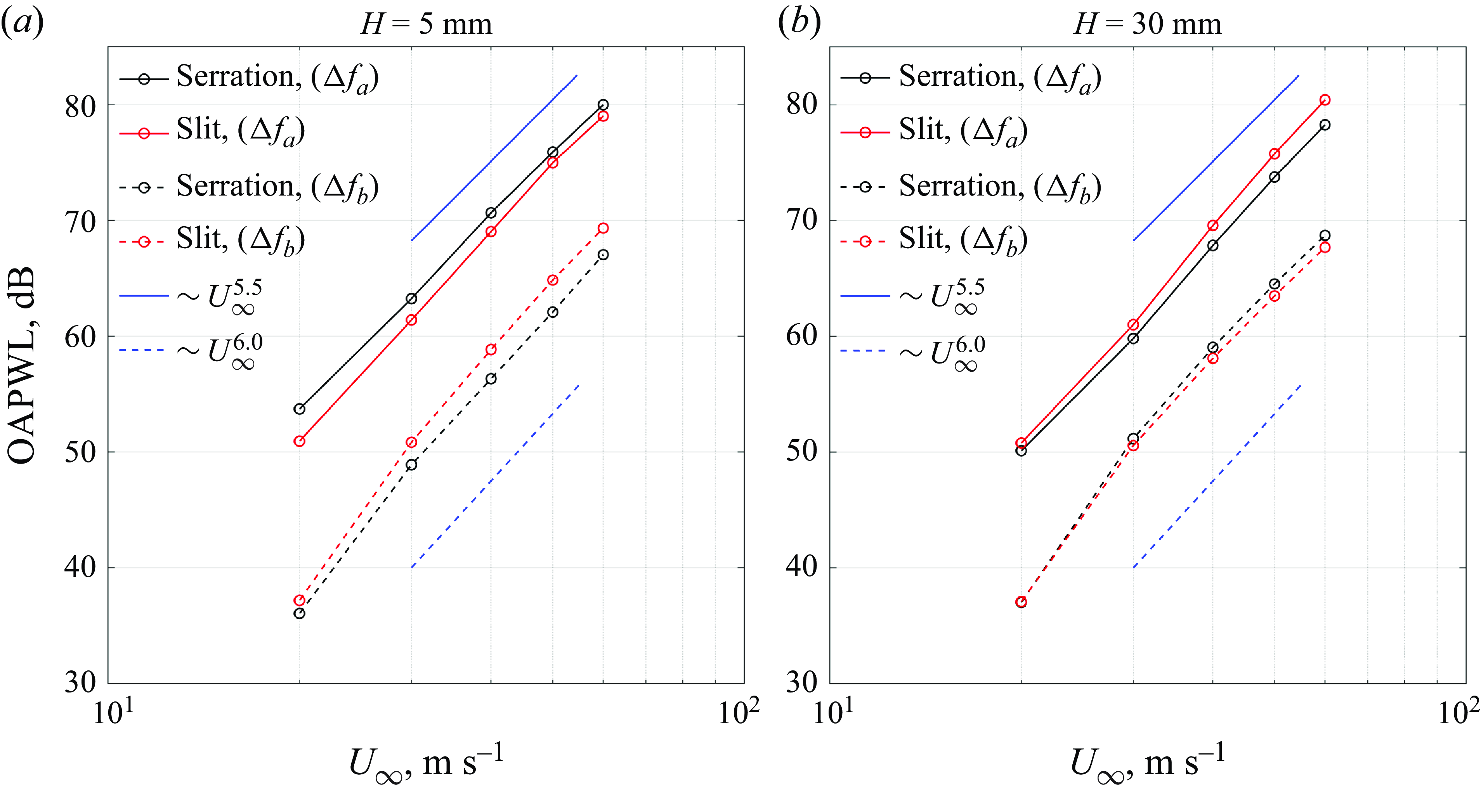
5.6. Slit trailing edge versus serrated sawtooth trailing edge
Following the demonstration of the frequency-tuning capability of the slit trailing edge, it is natural to explore whether its broadband noise reduction performance can match or even surpass that of the conventional sawtooth-type serrated trailing edge (hereafter simply referred to as the serrated trailing edge). This section aims to investigate the overall performance of the broadband noise reduction level in the context of the overall sound PWL (OAPWL), which can be defined as
 \begin{equation} {OAPWL} = 10\ \textrm {log}_{10} \left [\int _{\Delta f} \frac {\mathcal{W}(f)}{\mathcal{W}_0} {\rm d}f \right ]. \end{equation}
In this study, the OAPWL is obtained by integrating the sound power over a finite frequency range $\Delta f$
. Ideally, the
$\Delta f$
. Ideally, the $\Delta f$
should be as large as possible for a true representation of the overall noise performance. However, as shown in figure 7, noise increase is a dominant feature for the slit trailing edge at frequency above 4 kHz across the majority of H investigated here. The high frequency spectrum is likely to contain the turbulent scattering at the trailing edge and some extraneous noise sources, one of which is related to the strong cross-flow components at the slit gaps (demonstrated in § 4). Note that a similar cross-flow component also exists for a serrated trailing edge, as demonstrated in figure 12(d) of Gruber et al. (Reference Gruber, Joseph and Chong2011). For a meaningful comparison between the slit and serrated trailing edges, the analysis of the OAPWL is undertaken at two types of
$\Delta f$
should be as large as possible for a true representation of the overall noise performance. However, as shown in figure 7, noise increase is a dominant feature for the slit trailing edge at frequency above 4 kHz across the majority of H investigated here. The high frequency spectrum is likely to contain the turbulent scattering at the trailing edge and some extraneous noise sources, one of which is related to the strong cross-flow components at the slit gaps (demonstrated in § 4). Note that a similar cross-flow component also exists for a serrated trailing edge, as demonstrated in figure 12(d) of Gruber et al. (Reference Gruber, Joseph and Chong2011). For a meaningful comparison between the slit and serrated trailing edges, the analysis of the OAPWL is undertaken at two types of $\Delta f$
, where
$\Delta f$
, where $0.1 \lt \Delta f_a \lt 4$
kHz, and
$0.1 \lt \Delta f_a \lt 4$
kHz, and $4 \lt \Delta f_b \lt 20$
kHz. Note that
$4 \lt \Delta f_b \lt 20$
kHz. Note that $\Delta f_a$
and
$\Delta f_a$
and $\Delta f_b$
are designed to match the aforementioned acoustical-interference zone and high frequency zone, respectively.
$\Delta f_b$
are designed to match the aforementioned acoustical-interference zone and high frequency zone, respectively.
To serve as an appropriate comparison with the slit trailing edge, the serrated trailing edge must have the same $\lambda$
and H. On this basis, though the total wetted areas between them are not exactly identical, the deviation will be very small. Figure 13 shows the distributions of OAPWL against
$\lambda$
and H. On this basis, though the total wetted areas between them are not exactly identical, the deviation will be very small. Figure 13 shows the distributions of OAPWL against $U_\infty$
between the serrated and slit trailing edges for H = 5 and 30 mm. Both have the same
$U_\infty$
between the serrated and slit trailing edges for H = 5 and 30 mm. Both have the same $\lambda$
at 3.3 mm. Figures 13(a) and 13(b) contain the OAPWL obtained from frequency integration pertaining to the
$\lambda$
at 3.3 mm. Figures 13(a) and 13(b) contain the OAPWL obtained from frequency integration pertaining to the $\Delta f_a$
and
$\Delta f_a$
and $\Delta f_b$
, respectively. It is clear that the OAPWL (
$\Delta f_b$
, respectively. It is clear that the OAPWL ( $\Delta f_a$
), although underpinned by a smaller frequency range, still produces noise level that is approximately 10 dB larger than the OAPWL (
$\Delta f_a$
), although underpinned by a smaller frequency range, still produces noise level that is approximately 10 dB larger than the OAPWL ( $\Delta f_b$
) across the entire velocity range. This highlights that the main contributor to the OAPWL is the sound power radiated at low to medium frequency. This justifies the current analysis to ‘split’ the presentation of OAPWL in two different frequency categories.
$\Delta f_b$
) across the entire velocity range. This highlights that the main contributor to the OAPWL is the sound power radiated at low to medium frequency. This justifies the current analysis to ‘split’ the presentation of OAPWL in two different frequency categories.
Inspection of figure 13 reveals a velocity power-law scaling close to $U_\infty ^6$
at low velocities, which tends towards
$U_\infty ^6$
at low velocities, which tends towards $U_\infty ^{5.5}$
as the velocity increases. This classical behaviour has been discussed in Crighton & Leppington (Reference Crighton and Leppington1970), Ffowcs Williams & Hall (Reference Ffowcs Williams and Hall1970) and Blake (Reference Blake1986), where different velocity scaling exponents are associated with the compactness of the acoustic sources. Specifically, when the aerofoil is acoustically compact, a
$U_\infty ^{5.5}$
as the velocity increases. This classical behaviour has been discussed in Crighton & Leppington (Reference Crighton and Leppington1970), Ffowcs Williams & Hall (Reference Ffowcs Williams and Hall1970) and Blake (Reference Blake1986), where different velocity scaling exponents are associated with the compactness of the acoustic sources. Specifically, when the aerofoil is acoustically compact, a $U_\infty ^6$
scaling is expected, typical of compact dipole source. As flow speed increases and the source becomes acoustically extended, deviations from compact dipole behaviour can occur, leading to a less steep variation of OAPWL with flow speed. To further assess the compactness condition, the Helmholtz number
$U_\infty ^6$
scaling is expected, typical of compact dipole source. As flow speed increases and the source becomes acoustically extended, deviations from compact dipole behaviour can occur, leading to a less steep variation of OAPWL with flow speed. To further assess the compactness condition, the Helmholtz number $He=fc_\circ /U_\infty$
was calculated over the velocity range investigated here, where
$He=fc_\circ /U_\infty$
was calculated over the velocity range investigated here, where $c_\circ$
is the aerofoil chord length.
$c_\circ$
is the aerofoil chord length.
Figure 13 shows that the OAPWL, computed over the frequency bandwidth $0.1 \lt \Delta f_a \lt 4$
kHz, follows a velocity scaling law close to
$0.1 \lt \Delta f_a \lt 4$
kHz, follows a velocity scaling law close to $U_\infty ^{5.5}$
. This behaviour likely arises because, at a representative flow speed of 40 ms
$U_\infty ^{5.5}$
. This behaviour likely arises because, at a representative flow speed of 40 ms $^{-1}$
, the corresponding Helmholtz number spans a wide range,
$^{-1}$
, the corresponding Helmholtz number spans a wide range, $0.4 \lt He \lt 15$
, covering both compact and non-compact acoustic source regimes. As a result, the observed power law lies between the canonical
$0.4 \lt He \lt 15$
, covering both compact and non-compact acoustic source regimes. As a result, the observed power law lies between the canonical $U_\infty ^5$
and
$U_\infty ^5$
and $U_\infty ^6$
scalings, with
$U_\infty ^6$
scalings, with $U_\infty ^{5.5}$
representing an intermediate regime. In contrast, for the higher frequency range
$U_\infty ^{5.5}$
representing an intermediate regime. In contrast, for the higher frequency range $4 \lt \Delta f_b \lt 20$
kHz, the corresponding Helmholtz numbers fall within
$4 \lt \Delta f_b \lt 20$
kHz, the corresponding Helmholtz numbers fall within $15 \lt He \lt 75$
. Therefore, a higher scaling law of
$15 \lt He \lt 75$
. Therefore, a higher scaling law of $U_\infty ^6$
is observed, consistent with the aerofoil being extended over entire high frequency range.
$U_\infty ^6$
is observed, consistent with the aerofoil being extended over entire high frequency range.
For the slit trailing edge, it produces a lower level of OAPWL ( $\Delta f_a$
) than its serrated counterpart across the entire range of
$\Delta f_a$
) than its serrated counterpart across the entire range of $U_\infty$
when H = 5 mm. However, this trend reverses when H increases significantly to 30 mm. It is important to emphasise that this reversal in performance is primarily due to the serrated trailing edge being more sensitive to H in its influence on OAPWL (
$U_\infty$
when H = 5 mm. However, this trend reverses when H increases significantly to 30 mm. It is important to emphasise that this reversal in performance is primarily due to the serrated trailing edge being more sensitive to H in its influence on OAPWL ( $\Delta f_a$
). This observation is consistent with the findings of Gruber et al. (Reference Gruber, Joseph and Chong2011), who recommended that the length H of a serrated trailing edge should be greater, or at least of the same order as the local turbulent boundary layer thickness to achieve effective broadband noise reduction. For example, the serrated trailing edge with H = 5 mm is generally less effective than one with H = 30 mm in terms of noise reduction. In contrast, the slit trailing edge exhibits less sensitivity to H because its primary noise reduction mechanism relies on destructive wave interference.
$\Delta f_a$
). This observation is consistent with the findings of Gruber et al. (Reference Gruber, Joseph and Chong2011), who recommended that the length H of a serrated trailing edge should be greater, or at least of the same order as the local turbulent boundary layer thickness to achieve effective broadband noise reduction. For example, the serrated trailing edge with H = 5 mm is generally less effective than one with H = 30 mm in terms of noise reduction. In contrast, the slit trailing edge exhibits less sensitivity to H because its primary noise reduction mechanism relies on destructive wave interference.
For the OAPWL ( $\Delta f_b$
) as a function of
$\Delta f_b$
) as a function of $U_\infty$
, the comparison between the slit and serrated trailing edges shows an opposite trend. In the high frequency range, which contributes less to the overall OAPWL, a short serrated trailing edge proves more advantageous than a long one. In contrast, the OAPWL (
$U_\infty$
, the comparison between the slit and serrated trailing edges shows an opposite trend. In the high frequency range, which contributes less to the overall OAPWL, a short serrated trailing edge proves more advantageous than a long one. In contrast, the OAPWL ( $\Delta f_b$
) produced by the slit trailing edge remains relatively insensitive to H. Instead, the increase in noise at high frequencies for slit trailing edges is primarily influenced by
$\Delta f_b$
) produced by the slit trailing edge remains relatively insensitive to H. Instead, the increase in noise at high frequencies for slit trailing edges is primarily influenced by $\lambda$
, as discussed in previous sections.
$\lambda$
, as discussed in previous sections.
Variations of the $\Delta$
OAPWL pertaining to (a)
$\Delta$
OAPWL pertaining to (a) $\Delta f_a$
and (b)
$\Delta f_a$
and (b) $\Delta f_b$
, respectively, with
$\Delta f_b$
, respectively, with ${H}/{\delta ^*}$
, where
${H}/{\delta ^*}$
, where $\delta ^*$
is the measured turbulent boundary layer displacement thickness. The range of
$\delta ^*$
is the measured turbulent boundary layer displacement thickness. The range of $U_\infty$
investigated here includes 20
$U_\infty$
investigated here includes 20 $-$
60
$-$
60 $\textrm {m s}^{-1}$
. Note that
$\textrm {m s}^{-1}$
. Note that $\Delta$ ${\rm OAPWL} = {\rm OAPWL}_{(serration)} - \textrm {OAPWL}_{(slit)}$
.
${\rm OAPWL} = {\rm OAPWL}_{(serration)} - \textrm {OAPWL}_{(slit)}$
.

The next step is to determine a non-dimensional length scale ( $H/\delta ^*$
) that can be used as a criterion for the trailing edge optimisation in the context of
$H/\delta ^*$
) that can be used as a criterion for the trailing edge optimisation in the context of $\Delta {\rm OAPWL}$
. Here,
$\Delta {\rm OAPWL}$
. Here, $\delta ^*$
is the boundary layer displacement thickness for the baseline trailing edge measured in the experiment, and
$\delta ^*$
is the boundary layer displacement thickness for the baseline trailing edge measured in the experiment, and $\Delta {\rm OAPWL} = {\rm OAPWL}_{(serration)} - {\rm OAPWL}_{(slit)}$
. A positive value of
$\Delta {\rm OAPWL} = {\rm OAPWL}_{(serration)} - {\rm OAPWL}_{(slit)}$
. A positive value of $\Delta {\rm OAPWL}$
means that the slit trailing edge is quieter than the serrated trailing edge, and vice versa. Figure 14 shows the variations of the
$\Delta {\rm OAPWL}$
means that the slit trailing edge is quieter than the serrated trailing edge, and vice versa. Figure 14 shows the variations of the $\Delta {\rm OAPWL}$
pertaining to the
$\Delta {\rm OAPWL}$
pertaining to the $\Delta f_a$
and
$\Delta f_a$
and $\Delta f_b$
, respectively, against
$\Delta f_b$
, respectively, against ${H}/\delta ^*$
for
${H}/\delta ^*$
for $U_\infty = 20{-}60$ $\textrm {m s}^{-1}$
.
$\textrm {m s}^{-1}$
.
As demonstrated earlier, $\Delta f_a$
represents a frequency range whose sound power significantly contributes to the overall noise level. At
$\Delta f_a$
represents a frequency range whose sound power significantly contributes to the overall noise level. At $H/\delta ^* \lt 3$
, the slit trailing edge can be up to 3 dB quieter than the serrated trailing edge, demonstrating that slits outperform conventional sawtooth serrations only at small amplitudes. The observed trend is that as
$H/\delta ^* \lt 3$
, the slit trailing edge can be up to 3 dB quieter than the serrated trailing edge, demonstrating that slits outperform conventional sawtooth serrations only at small amplitudes. The observed trend is that as $H/\delta ^*$
decreases, the
$H/\delta ^*$
decreases, the $\Delta {\rm OAPWL}$
increases. This behaviour is attributed to the reduction in the longitudinal distance between the slit root and slit tip, which allows low frequency turbulent eddies to maintain higher streamwise coherence between these two geometrical discontinuities (as shown in figure 3 in § 4). This leads to
$\Delta {\rm OAPWL}$
increases. This behaviour is attributed to the reduction in the longitudinal distance between the slit root and slit tip, which allows low frequency turbulent eddies to maintain higher streamwise coherence between these two geometrical discontinuities (as shown in figure 3 in § 4). This leads to $\Delta p_r/\Delta p_t \rightarrow 1$
, thereby maximising the effectiveness of the destructive wave interference mechanism.
$\Delta p_r/\Delta p_t \rightarrow 1$
, thereby maximising the effectiveness of the destructive wave interference mechanism.
Unlike the serrated trailing edge, the slit trailing edge is less sensitive to variations in the boundary layer length scale. Importantly, the level of noise reduction achieved with slits increases with flow speed, due to the shorter convection time of turbulent eddies between the root and tip scattering locations and the resulting maintenance of higher coherence levels between them. In contrast, the performance of conventional sawtooth serrations tends to deteriorate with increasing flow speed. The results in figures 13 and 14 further highlight that a slit trailing edge with small H can continue to enhance noise reduction performance even at the highest inflow velocities investigated in this study.
When $H/\delta ^* \gt 3$
, serrated trailing edges outperform slit trailing edges, becoming quieter due to their improved noise reduction capability. This enhanced performance is achieved once a large
$H/\delta ^* \gt 3$
, serrated trailing edges outperform slit trailing edges, becoming quieter due to their improved noise reduction capability. This enhanced performance is achieved once a large $H/\delta ^*$
ratio is established, which is necessary for serrated trailing edges to function effectively. Additionally, the slit trailing edge is also influenced by constructive acoustic interference, a natural mechanism that appears to become more prominent at medium and large values of H, particularly for
$H/\delta ^*$
ratio is established, which is necessary for serrated trailing edges to function effectively. Additionally, the slit trailing edge is also influenced by constructive acoustic interference, a natural mechanism that appears to become more prominent at medium and large values of H, particularly for $St = 1.0$
, as shown in figure 7. The combined effects of these factors make the serrated trailing edge a more suitable choice for achieving effective noise reduction in this regime.
$St = 1.0$
, as shown in figure 7. The combined effects of these factors make the serrated trailing edge a more suitable choice for achieving effective noise reduction in this regime.
In summary, figure 14 clearly highlights the superior performance of slits compared with conventional serrations for relatively small H, where the destructive wave interference mechanism is the most effective. However, the trend reverses at large H, where conventional serrations outperform slits due to their enhanced sensitivity to boundary layer thickness, enabling more effective noise reduction in this regime. This distinction highlights the importance of selecting the appropriate trailing edge design based on the operating conditions and the target H/ $\delta ^*$
ratio to maximise noise reduction performance.
$\delta ^*$
ratio to maximise noise reduction performance.
For the $\Delta f_b$
, a frequency range whose sound power contributes less significantly to the overall noise level, the serrated trailing edge is consistently quieter than the slit trailing edge, except at high inflow velocity when
$\Delta f_b$
, a frequency range whose sound power contributes less significantly to the overall noise level, the serrated trailing edge is consistently quieter than the slit trailing edge, except at high inflow velocity when $H/\delta ^* \gt 5$
.
$H/\delta ^* \gt 5$
.
6. Further insight of the acoustical interference mechanism
If we revisit figure 10 for both the measured and predicted $\Delta$
SPL spectra, we can also observe an interesting phenomenon at
$\Delta$
SPL spectra, we can also observe an interesting phenomenon at $U_\infty$
= 60
$U_\infty$
= 60 $\textrm {m s}^{-1}$
. Whilst two peaks at
$\textrm {m s}^{-1}$
. Whilst two peaks at $St$
= 0.49 and 1.43, and a trough at
$St$
= 0.49 and 1.43, and a trough at $St$
= 1.04 in the measured
$St$
= 1.04 in the measured $\Delta$
SPL can be captured accurately by the predicted
$\Delta$
SPL can be captured accurately by the predicted $\Delta$
SPL, the measured spectrum also exhibits several extraneous peaks that occur at
$\Delta$
SPL, the measured spectrum also exhibits several extraneous peaks that occur at $St$
= 0.16, 0.73 and 0.96 whose characteristic Strouhal frequency cannot be predicted by the analytical noise model. The observation of a prominent
$St$
= 0.16, 0.73 and 0.96 whose characteristic Strouhal frequency cannot be predicted by the analytical noise model. The observation of a prominent $\Delta$
SPL peak at
$\Delta$
SPL peak at $St = 0.16$
is especially significant because it raises a prospect that noise reduction can be fine-tuned at very low frequency.
$St = 0.16$
is especially significant because it raises a prospect that noise reduction can be fine-tuned at very low frequency.
This phenomenon can be corroborated by re-examining the measured $\Delta$
PWL contour maps in figure 7. The noise reduction peaks, characterised by
$\Delta$
PWL contour maps in figure 7. The noise reduction peaks, characterised by $St \lt 0.5$
, can be consistently identified, particularly at high inflow velocities.
$St \lt 0.5$
, can be consistently identified, particularly at high inflow velocities.
The analytical noise model considers the acoustical interference between two compact sources at phase angle $n\pi$
, where n must be a natural number. If noise reduction is executed solely by the acoustic destructive interference, the lowest possible Strouhal frequency is 0.5. Therefore, the prominent noise reduction peak occurring at
$n\pi$
, where n must be a natural number. If noise reduction is executed solely by the acoustic destructive interference, the lowest possible Strouhal frequency is 0.5. Therefore, the prominent noise reduction peak occurring at $St \lt 0.5$
could be caused by the following reasons.
$St \lt 0.5$
could be caused by the following reasons.
-
(i) As discussed in § 4, high free stream velocity can give rise to some pressure-driven cross-flow components with strong streamwise vorticity at the slit’s suction surface. When the incoming turbulent eddies at the suction surface coalesce with the secondary flow structure, the ensuing lifting up and helical motions will result in an overall longer trajectory between the two scattering locations (
$H^\prime$
), which is greater than the physical dimension of the slit length H. -
(ii) At the suction surface,
$U_{c, {(slit)}} \lt U_{c, {(baseline)}}$
.


After combining both factors (i) and (ii), we will find that $H^\prime /U_{c, {(slit)}} \gt H/U_c$
at the slit’s suction surface. This means that the overall convection time of the turbulent eddies from one source (root) to another (tip) will be longer at the suction surface. On the other hand, using a simpler
$H^\prime /U_{c, {(slit)}} \gt H/U_c$
at the slit’s suction surface. This means that the overall convection time of the turbulent eddies from one source (root) to another (tip) will be longer at the suction surface. On the other hand, using a simpler $H/U_{c, {(baseline)}}$
remains accurate for the pressure surface slit due to the absence of secondary flow structure there.
$H/U_{c, {(baseline)}}$
remains accurate for the pressure surface slit due to the absence of secondary flow structure there.
To verify the above reasoning, We will select the case pertaining to that of figure 10 ( $U_\infty$
= 60
$U_\infty$
= 60 $\textrm {m s}^{-1}$
) and calculate the characteristics Strouhal numbers for noise reduction peaks based on (2.1) and (2.2). The predicted values will then be compared with the measured Strouhal numbers. The essence of this comparison is based on the premise that acoustic destructive interference will take place on the suction surface and pressure surface independently. More importantly, all the noise reduction peaks produced at the suction surface and pressure surface will be added to the
$\textrm {m s}^{-1}$
) and calculate the characteristics Strouhal numbers for noise reduction peaks based on (2.1) and (2.2). The predicted values will then be compared with the measured Strouhal numbers. The essence of this comparison is based on the premise that acoustic destructive interference will take place on the suction surface and pressure surface independently. More importantly, all the noise reduction peaks produced at the suction surface and pressure surface will be added to the $\Delta$
SPL spectrum.
$\Delta$
SPL spectrum.
Table 2 summarises the predicted and measured $St_{peak}$
using the convection time of
$St_{peak}$
using the convection time of $H/U_c$
pertaining to the acoustic destructive interference at the pressure surface. The agreement is shown to be excellent. The analytical model developed in this paper can also capture the
$H/U_c$
pertaining to the acoustic destructive interference at the pressure surface. The agreement is shown to be excellent. The analytical model developed in this paper can also capture the $St_{peak}$
well.
$St_{peak}$
well.


Next, the same approach is applied to the suction surface. In the absence of an accurate value for the turbulent eddies’ convection time at the suction surface, an empirical factor $\kappa$
is introduced such that
$\kappa$
is introduced such that $\kappa H/U_c \equiv H^\prime /U_{c, {(slit)}}$
. Table 3 summarises the predicted and measured
$\kappa H/U_c \equiv H^\prime /U_{c, {(slit)}}$
. Table 3 summarises the predicted and measured $St_{peak}$
values associated with acoustic destructive interference at the suction surface, using the convection time of
$St_{peak}$
values associated with acoustic destructive interference at the suction surface, using the convection time of $\kappa H/U_c$
, where
$\kappa H/U_c$
, where $\kappa = 3$
. Interestingly, all the predicted
$\kappa = 3$
. Interestingly, all the predicted $St_{peak}$
values match the measured ones. Note that the predicted
$St_{peak}$
values match the measured ones. Note that the predicted $St_{peak}$
values of 0.50 and 1.50 result from the application of natural numbers for
$St_{peak}$
values of 0.50 and 1.50 result from the application of natural numbers for $\kappa$
.
$\kappa$
.


The acoustic effects associated with trailing edge slits appear to depend not only on the geometrical configuration, but also on the underlying flow conditions, particularly the presence of cross-flow secondary structures. These structures are likely induced by a cross-stream pressure gradient at the slit, which can occur in lifting cambered aerofoils or symmetric aerofoils at non-zero angles of attack. Such secondary flows may interact with turbulent eddies in a way that enhances or suppresses certain acoustic modes, specifically, noise reduction via destructive interference at $St \lt 0.5$
, and noise amplification via constructive interference at
$St \lt 0.5$
, and noise amplification via constructive interference at $St \lt 1.0$
.
$St \lt 1.0$
.
To explore this mechanism further, we consider the case of a symmetric aerofoil at zero angle of attack, where no cross-stream pressure gradient, and hence no cross-flow secondary structure, is expected to develop at the trailing edge. In a separate but related study (Woodhead et al. Reference Woodhead, Scholz, Chong, Joseph, Chaitanya and Cabre2023), we investigated a configuration with a single row of holes placed at various streamwise positions $H$
relative to the trailing edge, but uniformly distributed along the span of a NACA0012 aerofoil at zero degrees angle of attack (see figure 15
a). This set-up is designed to activate similar interference mechanisms as a trailing edge slit, leading to periodic noise reduction at
$H$
relative to the trailing edge, but uniformly distributed along the span of a NACA0012 aerofoil at zero degrees angle of attack (see figure 15
a). This set-up is designed to activate similar interference mechanisms as a trailing edge slit, leading to periodic noise reduction at $St$
= 0.5, 1.5, … and noise amplification at
$St$
= 0.5, 1.5, … and noise amplification at $St$
= 1.0, 2.0, … .
$St$
= 1.0, 2.0, … .
(a) Geometrical parameters for a selective interference monoporous line (SIMPLE) trailing edge. The sources are defined as red (first source, $\Delta p_r$
) and blue (second source,
$\Delta p_r$
) and blue (second source, $\Delta p_t$
); (b) contour maps of the
$\Delta p_t$
); (b) contour maps of the $\Delta$
PWL in the
$\Delta$
PWL in the $f{-}H$
domains for a NACA0012 aerofoil with SIMPLE trailing edge at zero degree angle of attack between 20
$f{-}H$
domains for a NACA0012 aerofoil with SIMPLE trailing edge at zero degree angle of attack between 20 $\textrm {m s}^{-1}$ $\leq U_\infty \leq$
60
$\leq U_\infty \leq$
60 $\textrm {m s}^{-1}$
(Woodhead et al. Reference Woodhead, Scholz, Chong, Joseph, Chaitanya and Cabre2023).
$\textrm {m s}^{-1}$
(Woodhead et al. Reference Woodhead, Scholz, Chong, Joseph, Chaitanya and Cabre2023).

The resulting $\Delta$
PWL spectra, shown in figure 15(b), exhibit trends broadly consistent with those observed in slit configurations (figure 7). However, a notable difference is the absence of both the noise reduction at
$\Delta$
PWL spectra, shown in figure 15(b), exhibit trends broadly consistent with those observed in slit configurations (figure 7). However, a notable difference is the absence of both the noise reduction at $St \lt 0.5$
and the noise amplification at
$St \lt 0.5$
and the noise amplification at $St \lt 1.0$
. This observation suggests that while the primary mechanism of slitted aerofoil noise modulation is governed by acoustic interference between coherent sources near the root and tip, the presence of cross-flow secondary structures can influence the spectral characteristics of this interference.
$St \lt 1.0$
. This observation suggests that while the primary mechanism of slitted aerofoil noise modulation is governed by acoustic interference between coherent sources near the root and tip, the presence of cross-flow secondary structures can influence the spectral characteristics of this interference.
Further work is still needed to better understand the characteristics of $H^\prime$
and
$H^\prime$
and $U_{c, {(slit)}}$
at the slit’s suction surface in order to accurately determine the convection time for the turbulent eddies. Nevertheless, the simple analysis conducted in this section provides a strong indication that noise reduction at very low frequencies due to acoustic destructive interference is possible on slitted surfaces if large
$U_{c, {(slit)}}$
at the slit’s suction surface in order to accurately determine the convection time for the turbulent eddies. Nevertheless, the simple analysis conducted in this section provides a strong indication that noise reduction at very low frequencies due to acoustic destructive interference is possible on slitted surfaces if large $H^\prime$
and low
$H^\prime$
and low $U_{c, {(slit)}}$
occur either independently or simultaneously.
$U_{c, {(slit)}}$
occur either independently or simultaneously.
7. Concluding remarks
This study combines experimental and analytical efforts to investigate a novel, yet simple trailing edge treatment to enable aerofoil self-noise reduction with frequency-tuning capability. The physics behind the manipulation of the trailing edge noise radiation is based predominantly on the acoustical interference mechanism. Essentially, the trailing edge modification will facilitate a phase-cancellation of the acoustical pressure waves between two scattering sources that are physically separated in the longitudinal direction near the trailing edge. Unlike the conventional serrated-sawtooth trailing edge, which lacks the ability to target specific acoustical frequency due to the presence of multiple scattering sources along the oblique edges where no distinct phase angle can be established, a modification of the trailing edge in a ‘slitted’ geometry where the edges become parallel to the mean flow direction represents a better configuration to execute the acoustical interference mechanism.
For structurally rigid slit trailing edges, such as those studied here, acoustic scattering from the turbulent hydrodynamic sources along the slit edges, which are aligned with the main flow direction, become ineffective. In this case, the primary scattering sources are confined to the root and tip of the slit. Using a typical definition of a Strouhal number, and by forcing the condition of the acoustical destructive interference to establish the Strouhal number as 0.5, 1.5 and so on, one could fine-tune the peak frequency for the maximum noise reduction by adjusting the distance between the root and tip of the slit trailing edge. Another parameter that should be known a priori is the convection velocity of the turbulent eddies over the slit surfaces. The experimental and analytical results presented in this paper both positively verify this novel noise reduction method in what can be regarded as the frequency fine-tuning capability by a passive trailing edge noise control device. Measurement of the unsteady flow field near the slit surfaces also reveals a dominant cross-flow through the slit gap to form a pair of strong streamwise vortical structures on the suction surface of the slit trailing edge. The interaction between the turbulent eddies and these vortical structures can retard the convection velocity, thereby affecting the overall structure of the hydrodynamic–acoustical phase loop.
Understandably, at Strouhal number of 1.0, 2.0 and so on, the slit trailing edge can also trigger a constructive acoustical interference mechanism whereby it can radiate more efficiently than that of a baseline, straight trailing edge. Therefore, for a given slit trailing edge configuration, the radiated spectrum will feature an oscillatory behaviour pertaining to the noise reduction and noise increase across the entire frequency range. This oscillatory behaviour is well captured by the analytical model developed in this study. Therefore, trailing edge slits are particularly effective when noise is dominant within a narrow frequency range. However, when the noise to be reduced spans a broader spectrum, the overall noise reduction is only marginally better than that achieved with conventional serrations, especially at longer serration amplitudes.
An interesting feature pertaining to the slit trailing edge is also uncovered in this study. At a combined condition where both the inflow velocity and the slit length are large, the parameter used to non-dimensionalise the acoustical frequency, i.e. the convection time of the turbulent eddies, will need to be readjusted in order to capture all the tuned-frequencies pertaining to the noise reduction in the measured noise spectra. This implies that the overall structure of the hydrodynamic–acoustical phase loop might be altered by the change in dynamics of the cross-flow due to the high inflow velocity. Therefore, further level of noise reduction at very low frequency by acoustical interference can be achieved by increasing the convection time of the turbulent eddies. This represents an avenue to further improve the noise reduction capability for a slit trailing edge.
The results demonstrate that, for a slit trailing edge with a slit length less than three times the local turbulent boundary layer displacement thickness, it can outperform the serrated trailing edge in terms of the overall noise reduction covering the low to mid frequency range, up to the highest inflow velocity investigated here. This is simply because a smaller slit length can preserve better the coherent source strengths between the slit root and slit tip, which is an important criterion for executing the destructive wave interference. Consequently, industries such as the wind turbine manufacturers no longer need to rely on large amplitude serrated trailing edges for effective noise reduction. Instead, they can opt for shorter length trailing edge slits, which not only deliver superior noise reduction but also offer additional benefits, such as potentially smaller aerodynamic penalty due to their compact size, and frequency-tuning capability.
Funding
This work is supported by the UK Engineering and Physical Sciences Research Council (EPSRC) research grant (EP/N018737/1) ‘Quiet aerofoils of the next-generation’. We would also like to express our appreciation for the PhD studentship funded by the EPSRC Doctoral Training Partnership (DTP) awarded to P.C.W.
Declaration of interest
The authors report no conflict of interest.


 Open access