


1 Introduction
Let ${\widetilde {M}}$
be a complete simply connected Riemannian manifold with pinched negative sectional curvature at most
${\widetilde {M}}$
be a complete simply connected Riemannian manifold with pinched negative sectional curvature at most $-1$
. Let
$-1$
. Let $\Gamma $
be a nonelementary discrete subgroup of
$\Gamma $
be a nonelementary discrete subgroup of $\operatorname {Isom}({\widetilde {M}})$
, having involutions, that is, elements of order
$\operatorname {Isom}({\widetilde {M}})$
, having involutions, that is, elements of order $2$
. A loxodromic element of
$2$
. A loxodromic element of $\Gamma $
is strongly reversible if it is conjugated to its inverse by an involution of
$\Gamma $
is strongly reversible if it is conjugated to its inverse by an involution of $\Gamma $
. A strongly reversible closed geodesic in the Riemannian orbifold
$\Gamma $
. A strongly reversible closed geodesic in the Riemannian orbifold $M=\Gamma \backslash {\widetilde {M}}$
is the image of the translation axis of a strongly reversible loxodromic element of
$M=\Gamma \backslash {\widetilde {M}}$
is the image of the translation axis of a strongly reversible loxodromic element of $\Gamma $
. See [Reference O’Farrell and ShortO’FS] for a general discussion and an extensive review of reversibility phenomena in dynamical systems and group theory.
$\Gamma $
. See [Reference O’Farrell and ShortO’FS] for a general discussion and an extensive review of reversibility phenomena in dynamical systems and group theory.
In this paper, we give an asymptotic counting and equidistribution result of strongly reversible closed geodesics (with multiplicities and weights) of length at most $T\rightarrow +\infty $
, generalising results of [Reference SarnakSar, Reference Erlandsson and SoutoES]. We refer to Section 4 for the definition of the weights, that come from the thermodynamic formalism of equilibrium states, see for instance [Reference RuelleRue, Reference Paulin, Pollicott and SchapiraPPS]. In this Introduction, we restrict to the case where all weights are equal to
$T\rightarrow +\infty $
, generalising results of [Reference SarnakSar, Reference Erlandsson and SoutoES]. We refer to Section 4 for the definition of the weights, that come from the thermodynamic formalism of equilibrium states, see for instance [Reference RuelleRue, Reference Paulin, Pollicott and SchapiraPPS]. In this Introduction, we restrict to the case where all weights are equal to $1$
.
$1$
.
Strongly reversible closed geodesics appear for example in [Reference SarnakSar], where strongly reversible loxodromic elements of $\gamma \in \operatorname {PSL}_2({\mathbb Z})$
are called reciprocal elements because of their connections with the reciprocal integral binary quadratic forms of Gauss. See also [Reference Boca, Pasol, Popa and ZaharescuBoPPZ, Reference Bourgain and KontorovichBouK, Reference Basmajian and Suzzi ValliBaS1, Reference Basmajian and Suzzi ValliBaS2] for recent works on reciprocal elements of
$\gamma \in \operatorname {PSL}_2({\mathbb Z})$
are called reciprocal elements because of their connections with the reciprocal integral binary quadratic forms of Gauss. See also [Reference Boca, Pasol, Popa and ZaharescuBoPPZ, Reference Bourgain and KontorovichBouK, Reference Basmajian and Suzzi ValliBaS1, Reference Basmajian and Suzzi ValliBaS2] for recent works on reciprocal elements of $\operatorname {PSL}_2({\mathbb Z})$
. The same terminology is used for strongly reversible elements of Hecke triangle groups in [Reference Das and GongopadhyayDaG1], and for those in any lattice of
$\operatorname {PSL}_2({\mathbb Z})$
. The same terminology is used for strongly reversible elements of Hecke triangle groups in [Reference Das and GongopadhyayDaG1], and for those in any lattice of $\operatorname {PSL}_2({\mathbb R})$
that contains involutions in [Reference Erlandsson and SoutoES]. See Corollary 7.2 and Example 7.3, where we relate our results with [Reference SarnakSar, Thm. 2 (13)] and [Reference Erlandsson and SoutoES, Thm. 1.1].
$\operatorname {PSL}_2({\mathbb R})$
that contains involutions in [Reference Erlandsson and SoutoES]. See Corollary 7.2 and Example 7.3, where we relate our results with [Reference SarnakSar, Thm. 2 (13)] and [Reference Erlandsson and SoutoES, Thm. 1.1].
In order to state a simplified version of our counting and equidistribution result, we introduce the measures that come into play, referring to Section 4 for precise definitions, and to [Reference Broise-Alamichel, Parkkonen and PaulinBrPP] for more explanations and for historical references. We denote by $\|\mu \|$
the total mass of a measure
$\|\mu \|$
the total mass of a measure $\mu $
. We refer to Section 3 for the definition of the multiplicity of a strongly reversible closed geodesic. For instance, the multiplicity of a primitive strongly reversible closed geodesic is
$\mu $
. We refer to Section 3 for the definition of the multiplicity of a strongly reversible closed geodesic. For instance, the multiplicity of a primitive strongly reversible closed geodesic is $2$
, when
$2$
, when ${\widetilde {M}}$
has dimension
${\widetilde {M}}$
has dimension $2$
and the involutions in
$2$
and the involutions in $\Gamma $
only have isolated fixed points in
$\Gamma $
only have isolated fixed points in ${\widetilde {M}}$
.
${\widetilde {M}}$
.
Let $\delta _\Gamma $
be the critical exponent of
$\delta _\Gamma $
be the critical exponent of $\Gamma $
. Let
$\Gamma $
. Let $(\mu _{x})_{x\in {\widetilde {M}}}$
be a Patterson density for
$(\mu _{x})_{x\in {\widetilde {M}}}$
be a Patterson density for $\Gamma $
and let
$\Gamma $
and let $m_{\mathrm {BM}}$
be the associated Bowen-Margulis measure on
$m_{\mathrm {BM}}$
be the associated Bowen-Margulis measure on $T^1M=\Gamma \backslash T^1{\widetilde {M}}$
. When
$T^1M=\Gamma \backslash T^1{\widetilde {M}}$
. When $m_{\mathrm {BM}}$
is finite, then
$m_{\mathrm {BM}}$
is finite, then $\frac {m_{\mathrm {BM}}} {\|m_{\mathrm {BM}}\|}$
is the unique measure of maximal entropy for the geodesic flow on
$\frac {m_{\mathrm {BM}}} {\|m_{\mathrm {BM}}\|}$
is the unique measure of maximal entropy for the geodesic flow on $T^1M$
, see [Reference Otal and PeignéOtP, Reference Dilsavor and ThompsonDT]. When
$T^1M$
, see [Reference Otal and PeignéOtP, Reference Dilsavor and ThompsonDT]. When ${\widetilde {M}}$
is a symmetric space and
${\widetilde {M}}$
is a symmetric space and $\Gamma $
has finite covolume, then
$\Gamma $
has finite covolume, then $\mu _{x}$
is (up to a scalar multiple) the unique probability measure on
$\mu _{x}$
is (up to a scalar multiple) the unique probability measure on $\partial _\infty {\widetilde {M}}$
invariant under the stabiliser of x in the isometry group of
$\partial _\infty {\widetilde {M}}$
invariant under the stabiliser of x in the isometry group of ${\widetilde {M}}$
, and
${\widetilde {M}}$
, and $m_{\mathrm {BM}}$
is the Liouville measure, which is then finite and mixing. Given a nonempty, proper and totally geodesic submanifold D of
$m_{\mathrm {BM}}$
is the Liouville measure, which is then finite and mixing. Given a nonempty, proper and totally geodesic submanifold D of ${\widetilde {M}}$
, we denote by
${\widetilde {M}}$
, we denote by $\nu ^1 D$
its unit normal bundle, and by
$\nu ^1 D$
its unit normal bundle, and by ${\widetilde {\sigma }}^+_{D}$
(resp.
${\widetilde {\sigma }}^+_{D}$
(resp. ${\widetilde {\sigma }}^-_{D}$
) the outer (resp. inner) skinning measure on
${\widetilde {\sigma }}^-_{D}$
) the outer (resp. inner) skinning measure on $\nu ^1 D$
for
$\nu ^1 D$
for $\Gamma $
, which is the pull-back of the Patterson density by the map sending a normal vector to D to the point at
$\Gamma $
, which is the pull-back of the Patterson density by the map sending a normal vector to D to the point at $+\infty $
(resp.
$+\infty $
(resp. $-\infty $
) of the geodesic line it defines.
$-\infty $
) of the geodesic line it defines.
Let $I_\Gamma $
be the set of involutions of
$I_\Gamma $
be the set of involutions of $\Gamma $
that we assume to be nonempty. For every
$\Gamma $
that we assume to be nonempty. For every $\alpha \in I_\Gamma $
, let
$\alpha \in I_\Gamma $
, let $F_\alpha $
be its fixed point set in
$F_\alpha $
be its fixed point set in ${\widetilde {M}}$
. The group
${\widetilde {M}}$
. The group $\Gamma $
acts on
$\Gamma $
acts on $I_\Gamma $
by conjugation. Let I and J be fixed,
$I_\Gamma $
by conjugation. Let I and J be fixed, $\Gamma $
-invariant and nonempty subsets of
$\Gamma $
-invariant and nonempty subsets of $I_\Gamma $
. A loxodromic element
$I_\Gamma $
. A loxodromic element $\gamma $
of
$\gamma $
of $\Gamma $
, and its associated (oriented) closed geodesic in M, is
$\Gamma $
, and its associated (oriented) closed geodesic in M, is $\{I,J\}$
-reversible if
$\{I,J\}$
-reversible if $\gamma $
is conjugated to its inverse by an element
$\gamma $
is conjugated to its inverse by an element $\alpha $
of I such that
$\alpha $
of I such that $\gamma \alpha =\alpha \gamma ^{-1}\in J$
. Let
$\gamma \alpha =\alpha \gamma ^{-1}\in J$
. Let ${\mathcal {N}}_{I,J}(T)$
be the number of
${\mathcal {N}}_{I,J}(T)$
be the number of $\{I,J\}$
-reversible closed geodesics (counted with multiplicities, as defined in Section 3) of length at most T.
$\{I,J\}$
-reversible closed geodesics (counted with multiplicities, as defined in Section 3) of length at most T.
The $\Gamma $
-invariant measure
$\Gamma $
-invariant measure $\sum _{\alpha \in I} {\widetilde {\sigma }}^\pm _{F_\alpha }$
on
$\sum _{\alpha \in I} {\widetilde {\sigma }}^\pm _{F_\alpha }$
on $T^1{\widetilde {M}}$
induces a locally finite measure
$T^1{\widetilde {M}}$
induces a locally finite measure $\sigma ^\pm _{I}$
on
$\sigma ^\pm _{I}$
on $T^1M$
, called the skinning measure of the family
$T^1M$
, called the skinning measure of the family ${\mathcal {F}}_I=(F_\alpha )_{\alpha \in I}$
in
${\mathcal {F}}_I=(F_\alpha )_{\alpha \in I}$
in $T^1 M$
. When
$T^1 M$
. When ${\widetilde {M}}$
is a symmetric space and
${\widetilde {M}}$
is a symmetric space and $\Gamma $
has finite covolume, the measure
$\Gamma $
has finite covolume, the measure $\sigma ^\pm _{I}$
is nonzero. It is finite except when the fixed point set
$\sigma ^\pm _{I}$
is nonzero. It is finite except when the fixed point set $F_\alpha $
of some
$F_\alpha $
of some $\alpha \in I$
is a geodesic line with noncompact image in M. We refer to [Reference Parkkonen and PaulinPP6, Reference Parkkonen, Paulin and SayousParPS] and the end of Example 7.4 for further information on the surprising counting phenomena and growth that occur when the skinning measures are infinite.
$\alpha \in I$
is a geodesic line with noncompact image in M. We refer to [Reference Parkkonen and PaulinPP6, Reference Parkkonen, Paulin and SayousParPS] and the end of Example 7.4 for further information on the surprising counting phenomena and growth that occur when the skinning measures are infinite.
Theorem 1.1. Assume that the Bowen-Margulis measure $m_{\mathrm {BM}}$
is finite and mixing for the geodesic flow on
$m_{\mathrm {BM}}$
is finite and mixing for the geodesic flow on $ T^1M$
, and that the skinning measures
$ T^1M$
, and that the skinning measures $\sigma ^+_{I}$
and
$\sigma ^+_{I}$
and $\sigma ^-_{J}$
are finite nonzero.
$\sigma ^-_{J}$
are finite nonzero.
-
(1) As $T\rightarrow +\infty $
, we have
$T\rightarrow +\infty $
, we have -
(2) When
$J=I$
, the sum (with multiplicities) of the Lebesgue measures along the
$\{I,I\}$
-reversible closed geodesics of length at most T, normalised to be a probability measure and lifted to
$T^1M$
, weak-star converges on
$T^1M$
to the Bowen-Margulis measure
$m_{\mathrm {BM}}$
, normalised to be a probability measure.


The proof of Theorem 1.1 relates strongly reversible closed geodesics to common perpendiculars between the fixed point sets of involutions of $\Gamma $
, as explained in Section 2, and then uses the counting and equidistribution results of [Reference Parkkonen and PaulinPP3, Reference Broise-Alamichel, Parkkonen and PaulinBrPP, Reference Parkkonen and PaulinPP5], with subtle work on multiplicities in the new averaging arguments. The exponential growth rate
$\Gamma $
, as explained in Section 2, and then uses the counting and equidistribution results of [Reference Parkkonen and PaulinPP3, Reference Broise-Alamichel, Parkkonen and PaulinBrPP, Reference Parkkonen and PaulinPP5], with subtle work on multiplicities in the new averaging arguments. The exponential growth rate $\frac {\delta _\Gamma }{2}$
of
$\frac {\delta _\Gamma }{2}$
of ${\mathcal {N}}_{I,J}(T)$
is half the exponential growth rate
${\mathcal {N}}_{I,J}(T)$
is half the exponential growth rate $\delta _\Gamma $
of the total number of closed geodesics in M. This can be understood by seeing the
$\delta _\Gamma $
of the total number of closed geodesics in M. This can be understood by seeing the $\{I,J\}$
-reversible closed geodesics as playing ping-pong between the fixed point set of an element of I and the fixed point set of an element of J. The (finite) intersection of the stabilisers of these two (disjoint) fixed point sets plays a role in the above counting problem, hence forces the introduction of multiplicities in Section 3. This is in accordance with the general problem of counting objects having symmetries, the (inverse of the) orders of the symmetry groups have to come into play for naturality purposes.
$\{I,J\}$
-reversible closed geodesics as playing ping-pong between the fixed point set of an element of I and the fixed point set of an element of J. The (finite) intersection of the stabilisers of these two (disjoint) fixed point sets plays a role in the above counting problem, hence forces the introduction of multiplicities in Section 3. This is in accordance with the general problem of counting objects having symmetries, the (inverse of the) orders of the symmetry groups have to come into play for naturality purposes.
Let ${{\mathbb H}}^2_{\mathbb R}$
be the upper halfspace model of the real hyperbolic plane, let
${{\mathbb H}}^2_{\mathbb R}$
be the upper halfspace model of the real hyperbolic plane, let $\Gamma _6$
be the Hecke triangle group of signature
$\Gamma _6$
be the Hecke triangle group of signature $(2,6,\infty )$
and let I be the set of conjugates in
$(2,6,\infty )$
and let I be the set of conjugates in $\Gamma _6$
of the involution
$\Gamma _6$
of the involution $z\mapsto -\frac 1z$
. Figure 1 on the left (resp. right) shows the
$z\mapsto -\frac 1z$
. Figure 1 on the left (resp. right) shows the $\{I,I\}$
-reversible closed geodesics of
$\{I,I\}$
-reversible closed geodesics of $\Gamma _6\backslash {{\mathbb H}}^2_{\mathbb R}$
of length at most
$\Gamma _6\backslash {{\mathbb H}}^2_{\mathbb R}$
of length at most $11$
(resp.
$11$
(resp. $13$
) restricted to the low part of the standard fundamental polygon of
$13$
) restricted to the low part of the standard fundamental polygon of $\Gamma _6$
. See Example 7.3 for more information.
$\Gamma _6$
. See Example 7.3 for more information.
Equidistribution of reversible closed geodesics in $\Gamma _6\backslash {{\mathbb H}}^2_{\mathbb R}$
.
$\Gamma _6\backslash {{\mathbb H}}^2_{\mathbb R}$
.

The collection of periodic orbits considered in Theorem 1.1 (2) is a strict subset of the collection of all periodic orbits (known to equidistribute to the Bowen-Margulis measure by results of [Reference BowenBow] and [Reference RoblinRob]). The collection of $\{I,I\}$
-reversible closed geodesics of length at most T grows at a rate
$\{I,I\}$
-reversible closed geodesics of length at most T grows at a rate $c\, e^{\frac {\delta _\Gamma }{2}T}$
, which is considerably smaller than the growth
$c\, e^{\frac {\delta _\Gamma }{2}T}$
, which is considerably smaller than the growth $c'\,T^{-1}\, e^{\delta _\Gamma \,T}$
of the set of closed geodesics of length at most T, where
$c'\,T^{-1}\, e^{\delta _\Gamma \,T}$
of the set of closed geodesics of length at most T, where $c,c'$
are constants.
$c,c'$
are constants.
The equidistribution of reciprocal geodesics on $\operatorname {PSL}_2({\mathbb Z})\backslash {{\mathbb H}}^2_{\mathbb R}$
was conjectured by Sarnak in [Reference SarnakSar], and proved for lattices of
$\operatorname {PSL}_2({\mathbb Z})\backslash {{\mathbb H}}^2_{\mathbb R}$
was conjectured by Sarnak in [Reference SarnakSar], and proved for lattices of $\operatorname {PSL}_2({\mathbb R})$
that contain involutions by Erlandsson and Souto in [Reference Erlandsson and SoutoES]. When
$\operatorname {PSL}_2({\mathbb R})$
that contain involutions by Erlandsson and Souto in [Reference Erlandsson and SoutoES]. When ${\widetilde {M}}$
is a symmetric space and
${\widetilde {M}}$
is a symmetric space and $\Gamma $
is an arithmetic lattice, we furthermore have error terms in both the counting and equidistribution statements of Theorem 1.1 (see Sections 5 and 6). The constant
$\Gamma $
is an arithmetic lattice, we furthermore have error terms in both the counting and equidistribution statements of Theorem 1.1 (see Sections 5 and 6). The constant $\frac {\|\sigma ^+_{I}\|\, \|\sigma ^-_{J}\|}{\delta _\Gamma \, \|m_{\mathrm {BM}}\|}$
may be made explicit in these cases (see Section 7). We recover Theorems 1.1 and 1.4 of [Reference Erlandsson and SoutoES] for the particular case of the real hyperbolic plane
$\frac {\|\sigma ^+_{I}\|\, \|\sigma ^-_{J}\|}{\delta _\Gamma \, \|m_{\mathrm {BM}}\|}$
may be made explicit in these cases (see Section 7). We recover Theorems 1.1 and 1.4 of [Reference Erlandsson and SoutoES] for the particular case of the real hyperbolic plane ${\widetilde {M}}={\mathbb H}^2_{\mathbb R}$
and
${\widetilde {M}}={\mathbb H}^2_{\mathbb R}$
and $I=J=I_\Gamma $
in a synthetic way, adding an error term to their result.
$I=J=I_\Gamma $
in a synthetic way, adding an error term to their result.
We conclude this introduction with applications of Theorem 1.1. We refer to Section 7 for more examples, in particular to Subsection 7.2 for a study of strongly reversible closed geodesics in complex hyperbolic reflection groups, as examplified by Deraux’s example 7.8.
Corollary 1.2. Let $(W,S)$
be a real hyperbolic Coxeter reflection system in dimension
$(W,S)$
be a real hyperbolic Coxeter reflection system in dimension $n\geq 2$
with a finite volume Coxeter polyhedron P that is compact if
$n\geq 2$
with a finite volume Coxeter polyhedron P that is compact if $n=2$
. Let
$n=2$
. Let $I_S$
be the set of the conjugates by elements of W of the elements of S. Then there exists
$I_S$
be the set of the conjugates by elements of W of the elements of S. Then there exists $\kappa>0$
such that, as
$\kappa>0$
such that, as $T\rightarrow +\infty $
, we have
$T\rightarrow +\infty $
, we have
 $$\begin{align*}\frac{1}{2}{\mathcal{N}}_{I_S,I_S}(T)=\frac{\operatorname{Vol}(\partial P)^2} {(n-1)\,2^n\operatorname{Vol}({\mathbb S}^{n-1})\operatorname{Vol}(P)} \;e^{\frac{n-1}2\,T} \big(1+\operatorname{O}(e^{-\kappa T})\big)\,. \end{align*}$$
We recall that the fixed point set in ${{\mathbb H}}^n_{\mathbb R}$
of a conjugate of an element of S is a wall of the Coxeter system
${{\mathbb H}}^n_{\mathbb R}$
of a conjugate of an element of S is a wall of the Coxeter system $(W,S)$
. A loxodromic element of W is
$(W,S)$
. A loxodromic element of W is $\{I_S,I_S\}$
-reversible if its translation axis meets two walls perpendicularly. The key idea of the proof is to reduce the counting of strongly reversible closed geodesics in
$\{I_S,I_S\}$
-reversible if its translation axis meets two walls perpendicularly. The key idea of the proof is to reduce the counting of strongly reversible closed geodesics in $W\backslash {{\mathbb H}}^n_{\mathbb R}$
to the counting of common perpendiculars between walls, the upper bound on the lengths of the common perpendiculars being one half of the upper bound on the lengths of the closed geodesics. This is technically not so easy since a given translation axis can meet lots of walls. The proof also requires a computation of the skinning measures of the family of walls, which turns out to be nicely related to the total volume of the faces of the Coxeter polyhedron P.
$W\backslash {{\mathbb H}}^n_{\mathbb R}$
to the counting of common perpendiculars between walls, the upper bound on the lengths of the common perpendiculars being one half of the upper bound on the lengths of the closed geodesics. This is technically not so easy since a given translation axis can meet lots of walls. The proof also requires a computation of the skinning measures of the family of walls, which turns out to be nicely related to the total volume of the faces of the Coxeter polyhedron P.
Corollary 1.2 is not applicable if $n=2$
and P is not compact, see [Reference Parkkonen and PaulinPP6] and Example 7.4 for further information. For example,
$n=2$
and P is not compact, see [Reference Parkkonen and PaulinPP6] and Example 7.4 for further information. For example,
 $$\begin{align*}P=\big\{(z,t)\in{{\mathbb H}}^3_{\mathbb R}={\mathbb C}\times{\mathbb R}_+: 0\le\operatorname{Re}(z) \leq \frac{1}{2}\,,\ 0\le \operatorname{Im }(z) \leq \frac{1}{2}\ \textrm{and}\ |z|^2+t^2\geq 1\big\} \end{align*}$$
is a finite volume Coxeter polyhedron in the upper halfspace model ${{\mathbb H}}^3_{\mathbb R}$
of the real hyperbolic
${{\mathbb H}}^3_{\mathbb R}$
of the real hyperbolic $3$
-space. The dihedral angles between two vertical faces of P are
$3$
-space. The dihedral angles between two vertical faces of P are $\pi /2$
and the dihedral angles of the edges of the spherical face of P are
$\pi /2$
and the dihedral angles of the edges of the spherical face of P are $\pi /3$
. Figure 2 shows some of the boundaries at infinity of the walls of the Coxeter system
$\pi /3$
. Figure 2 shows some of the boundaries at infinity of the walls of the Coxeter system $(W,S)$
generated by reflections in the (codimension
$(W,S)$
generated by reflections in the (codimension $1$
) faces of P. See Example 7.5 for further information.
$1$
) faces of P. See Example 7.5 for further information.
Boundaries at infinity of walls of the Coxeter system with Coxeter polyhedron P.

In Sections 5 and 6, we prove more general versions of the counting and equidistribution results stated in Theorem 1.1, with potentials coming from the thermodynamic formalism of equilibrium states, see [Reference Paulin, Pollicott and SchapiraPPS], including a version of Theorem 1.1 for simplicial trees. An application of the case of trees is given by the following result. We refer to Subsection 7.3 for the proof of this result, and for the relevant definitions.
Corollary 1.3. Let q be a prime power with $q\equiv 3\bmod 4$
. Let
$q\equiv 3\bmod 4$
. Let $\Gamma =\operatorname {PGL}_2({\mathbb F}_q[Y])$
and let
$\Gamma =\operatorname {PGL}_2({\mathbb F}_q[Y])$
and let $I_\alpha $
be the conjugacy class in
$I_\alpha $
be the conjugacy class in $\Gamma $
of the involution
$\Gamma $
of the involution ![]() . The number
. The number ${\mathcal {N}}_{I_\alpha ,I_\alpha }(n)$
of conjugacy classes (counted with multiplicities) of
${\mathcal {N}}_{I_\alpha ,I_\alpha }(n)$
of conjugacy classes (counted with multiplicities) of $\{I_\alpha , I_\alpha \}$
-reversible loxodromic elements of
$\{I_\alpha , I_\alpha \}$
-reversible loxodromic elements of $\Gamma $
, whose translation length on the Bruhat-Tits tree of
$\Gamma $
, whose translation length on the Bruhat-Tits tree of $(\operatorname {PGL}_2, {\mathbb F}_q((Y^{-1})))$
is at most n, satisfies, as
$(\operatorname {PGL}_2, {\mathbb F}_q((Y^{-1})))$
is at most n, satisfies, as $n\in 4{\mathbb Z}$
tends to
$n\in 4{\mathbb Z}$
tends to $+\infty $
,
$+\infty $
,

Now that the thermodynamic formalism has been appropriately extended to CAT $(-1)$
-spaces in [Reference Dilsavor and ThompsonDT], we think that results analogous to the ones of this paper could be true for general proper CAT
$(-1)$
-spaces in [Reference Dilsavor and ThompsonDT], we think that results analogous to the ones of this paper could be true for general proper CAT $(-1)$
-spaces such as hyperbolic buildings with discrete groups of isometries having involutions. It would require first the extension of the results of [Reference Parkkonen and PaulinPP3] to this more general setting. This could be an interesting project, that we won’t pursue due to lack of time and energy.
$(-1)$
-spaces such as hyperbolic buildings with discrete groups of isometries having involutions. It would require first the extension of the results of [Reference Parkkonen and PaulinPP3] to this more general setting. This could be an interesting project, that we won’t pursue due to lack of time and energy.
2 Strongly reversible elements and common perpendiculars
Let X be
-
• either a complete simply connected Riemannian manifold
${\widetilde {M}}$
with dimension at least
$2$
and with pinched negative sectional curvature
$-a^2\leq K\leq -1$
, -
• or the geometric realisation of a simplicial tree
${\mathbb X}$
without terminal vertices and with uniformly bounded degrees of vertices.


We denote by $X\cup \partial _\infty X$
the geometric compactification of X, where
$X\cup \partial _\infty X$
the geometric compactification of X, where $\partial _\infty X$
is the boundary at infinity of X. For every closed convex subset A of X, we denote by
$\partial _\infty X$
is the boundary at infinity of X. For every closed convex subset A of X, we denote by $\overline {A}$
its closure in
$\overline {A}$
its closure in $X\cup \partial _\infty X$
.
$X\cup \partial _\infty X$
.
When X is a manifold, we denote by $\operatorname {Isom}(X)$
its locally compact full isometry group. When X is a tree, we denote by
$\operatorname {Isom}(X)$
its locally compact full isometry group. When X is a tree, we denote by $\operatorname {Isom}(X)$
the locally compact group of automorphisms of
$\operatorname {Isom}(X)$
the locally compact group of automorphisms of ${\mathbb X}$
without edge inversion. Let
${\mathbb X}$
without edge inversion. Let $\Gamma $
be a nonelementary discrete subgroup of
$\Gamma $
be a nonelementary discrete subgroup of $\operatorname {Isom}(X)$
. An element in
$\operatorname {Isom}(X)$
. An element in $\operatorname {Isom}(X)$
of order
$\operatorname {Isom}(X)$
of order $2$
is called an involution. We assume from now on that
$2$
is called an involution. We assume from now on that $\Gamma $
contains involutions. See for instance [Reference Bridson and HaefligerBrH] for background on
$\Gamma $
contains involutions. See for instance [Reference Bridson and HaefligerBrH] for background on $\operatorname {CAT}(-1)$
spaces and their discrete groups of isometries, and [Reference SerreSer] for background on group actions on trees, as well as [Reference Broise-Alamichel, Parkkonen and PaulinBrPP, Chap. 2].
$\operatorname {CAT}(-1)$
spaces and their discrete groups of isometries, and [Reference SerreSer] for background on group actions on trees, as well as [Reference Broise-Alamichel, Parkkonen and PaulinBrPP, Chap. 2].
For every $\gamma \in \operatorname {Isom}(X)$
, we denote by
$\gamma \in \operatorname {Isom}(X)$
, we denote by
 $$\begin{align*}\lambda(\gamma)=\inf_{x\in X} d(x,\gamma x) \end{align*}$$
the translation length of $\gamma $
. The element
$\gamma $
. The element $\gamma $
is loxodromic if
$\gamma $
is loxodromic if $\lambda (\gamma )>0$
. We then denote its translation axis by
$\lambda (\gamma )>0$
. We then denote its translation axis by
 $$\begin{align*}\operatorname{Ax}_\gamma=\{x\in X:d(x,\gamma x)=\lambda(\gamma)\}\,, \end{align*}$$
and its repelling, attracting fixed points at infinity by $\gamma _-,\gamma _+ \in \partial _\infty X$
respectively. The element
$\gamma _-,\gamma _+ \in \partial _\infty X$
respectively. The element $\gamma $
is elliptic if it has a fixed point in X and parabolic if it is neither loxodromic nor elliptic.
$\gamma $
is elliptic if it has a fixed point in X and parabolic if it is neither loxodromic nor elliptic.
The discrete group $\Gamma $
acts by conjugation on the nonempty set
$\Gamma $
acts by conjugation on the nonempty set $I_\Gamma $
of involutions of
$I_\Gamma $
of involutions of $\Gamma $
. In what follows, I and J will denote two fixed,
$\Gamma $
. In what follows, I and J will denote two fixed, $\Gamma $
-invariant and nonempty subsets of
$\Gamma $
-invariant and nonempty subsets of $I_\Gamma $
, and will be endowed with the left action by conjugation of
$I_\Gamma $
, and will be endowed with the left action by conjugation of $\Gamma $
. For instance, given an involution
$\Gamma $
. For instance, given an involution $\alpha $
of
$\alpha $
of $\Gamma $
, the set of the conjugates of
$\Gamma $
, the set of the conjugates of $\alpha $
by the elements of
$\alpha $
by the elements of $\Gamma $
will be denoted by
$\Gamma $
will be denoted by $I_\alpha $
.
$I_\alpha $
.
Let $\alpha \in I_\Gamma $
. We denote by
$\alpha \in I_\Gamma $
. We denote by
 $$\begin{align*}F_\alpha=\{x\in X:\alpha x =x\} \end{align*}$$
the fixed point set of $\alpha $
, which is a proper, nonempty,Footnote 1
closed and convexFootnote 2
subset of X. It is a totally geodesic submanifold when X is a manifold by for instance [Reference Gallot, Hulin and LafontaineGHL, §2.80 bis], and the geometric realisation of a simplicial subtree of
$\alpha $
, which is a proper, nonempty,Footnote 1
closed and convexFootnote 2
subset of X. It is a totally geodesic submanifold when X is a manifold by for instance [Reference Gallot, Hulin and LafontaineGHL, §2.80 bis], and the geometric realisation of a simplicial subtree of ${\mathbb X}$
when X is a tree.
${\mathbb X}$
when X is a tree.
Remark 2.1.
-
(1) If
$X={\widetilde {M}}$
is a manifold with dimension
$m\geq 1$
, for
$\alpha \in \operatorname {Isom}(X)$
an involution, the dimension k of the submanifold
$F_\alpha $
could be any element
$k\in [\!\![ 0, m-1 ]\!\!]$
,Footnote 3
as can be seen when
${\widetilde {M}}$
is the real hyperbolic m-space
${\mathbb H}^m_{\mathbb R}$
. For every
$x\in F_\alpha $
, the tangent space
$T_x {\widetilde {M}}$
decomposes as an orthogonal sum
$T_x{\widetilde {M}}= T_xF_\alpha \oplus \nu _xF_\alpha $
of the k-dimensional tangent space
$T_xF_\alpha $
and the
$(m-k)$
-dimensional normal space
$\nu _x F_\alpha $
at x to the fixed point set
$F_\alpha $
. The tangent map
$T_x\alpha $
acts by the block matrix on this decomposition of
$T_x{\widetilde {M}}$
. Thus, the involution
$\alpha $
reverses the orientation of
${\widetilde {M}}$
if and only if
$m-k$
is odd. -
(2) If
$X={\widetilde {M}}$
is a manifold, then the action of any
$\alpha \in I_\Gamma $
on
${\widetilde {M}}$
is determined by
$F_\alpha $
: Indeed, if
$$\begin{align*}\forall\;\alpha,\beta\in I_\Gamma,\qquad\text{if}\quad F_\alpha=F_\beta\quad\text{then}\quad\alpha=\beta\,. \end{align*}$$
$x\in F_\alpha $
, then
$\alpha x=x$
, and if
$x\in {\widetilde {M}} - F_\alpha $
, if p is the closest point to x on
$F_\alpha $
, then
$\alpha x$
is the symmetric point of x with respect to p on the (unique) geodesic line through x and p. But this is no longer true when X is a tree, see the comment after Lemma 2.6, and Lemma 7.9.


An element $\gamma \in \Gamma $
is reversible in
$\gamma \in \Gamma $
is reversible in $\Gamma $
if it is conjugated to its inverse. It is strongly reversible in
$\Gamma $
if it is conjugated to its inverse. It is strongly reversible in $\Gamma $
if it is conjugated to its inverse by an involution in
$\Gamma $
if it is conjugated to its inverse by an involution in $\Gamma $
. We refer to [Reference O’Farrell and ShortO’FS, Sect. 2] for the basic ideas of reversibility, and the rest of the cited book for an extensive survey. In particular, an element of
$\Gamma $
. We refer to [Reference O’Farrell and ShortO’FS, Sect. 2] for the basic ideas of reversibility, and the rest of the cited book for an extensive survey. In particular, an element of $\Gamma $
is strongly reversible if and only if it is the product of two involutions of
$\Gamma $
is strongly reversible if and only if it is the product of two involutions of $\Gamma $
, see [Reference O’Farrell and ShortO’FS, Prop. 2.12]. An element
$\Gamma $
, see [Reference O’Farrell and ShortO’FS, Prop. 2.12]. An element $\gamma \in \Gamma $
is
$\gamma \in \Gamma $
is $\{I,J\}$
-reversible if there exists an element
$\{I,J\}$
-reversible if there exists an element $\alpha \in I$
such that we have
$\alpha \in I$
such that we have $\gamma \alpha =\alpha \gamma ^{-1} \in J$
. Such an element
$\gamma \alpha =\alpha \gamma ^{-1} \in J$
. Such an element $\alpha \in I_{\Gamma }$
is called a
$\alpha \in I_{\Gamma }$
is called a $\gamma $
-reversing involution for
$\gamma $
-reversing involution for $(I,J)$
.
$(I,J)$
.
In this paper, we are interested in strongly reversible and loxodromic elements of $\Gamma $
. We denote by
$\Gamma $
. We denote by ${\widetilde {\mathfrak R}}_{I,J}$
the set of
${\widetilde {\mathfrak R}}_{I,J}$
the set of $\{I,J\}$
-reversible loxodromic elements of
$\{I,J\}$
-reversible loxodromic elements of $\Gamma $
. Note that if
$\Gamma $
. Note that if $I'$
and
$I'$
and $J'$
are
$J'$
are $\Gamma $
-invariant subsets of
$\Gamma $
-invariant subsets of $I_\Gamma $
such that
$I_\Gamma $
such that $I\subset I'$
and
$I\subset I'$
and $J\subset J'$
, then
$J\subset J'$
, then ${\widetilde {\mathfrak R}}_{I,J}\subset {\widetilde {\mathfrak R}}_{I',J'}$
.
${\widetilde {\mathfrak R}}_{I,J}\subset {\widetilde {\mathfrak R}}_{I',J'}$
.
Remark 2.2.
-
(1) Given a
$\gamma $
-reversing involution
$\alpha $
for
$(I,J)$
, the set of
$\gamma $
-reversing involutions for
$(I,J)$
is equal to
$\{\alpha '\in (\alpha Z_\Gamma (\gamma ) )\cap I:\gamma \alpha '\in J\}$
. Since
$\beta '\alpha '=(\beta '\alpha '{\beta '}^{-1})\beta '$
for all
$\alpha '\in I$
and
$\beta '\in J$
, the element
$\beta =\gamma \alpha $
is a
$\gamma $
-reversing involution for
$(J,I)$
. Therefore being
$\{I,J\}$
-reversible or
$\{J,I\}$
-reversible is equivalent, thus explaining the notation. In particular, the set
${\widetilde {\mathfrak R}}_{I,J}$
is invariant under taking inverses. -
(2) The left action of
$\Gamma $
on itself by conjugation preserves
${\widetilde {\mathfrak R}}_{I,J}$
, since for every
$\delta \in \Gamma $
, an involution
$\alpha $
is
$\gamma $
-reversing for
$(I,J)$
if and only if the element
$\delta \alpha \delta ^{-1}$
, which belongs to I, is
$\delta \gamma \delta ^{-1}$
-reversing for
$(I,J)$
, as
$$\begin{align*}(\delta \alpha \delta^{-1})(\delta \gamma \delta^{-1})(\delta \alpha\delta^{-1})^{-1} = (\delta \gamma \delta^{-1}) ^{-1} \quad\text{and}\quad (\delta\gamma \delta^{-1})(\delta \alpha\delta^{-1}) = \delta (\gamma\alpha) \delta^{-1}\in J\;. \end{align*}$$
-
(3) The set
${\widetilde {\mathfrak R}}_{I,J}$
of
$\{I,J\}$
-reversible loxodromic elements of
$\Gamma $
is invariant by taking odd powers: Indeed, let
$\gamma \in {\widetilde {\mathfrak R}}_{I,J}$
and let
$\alpha $
be a
$\gamma $
-reversing involution for
$(I,J)$
, so that
$\alpha \in I$
,
$\beta =\gamma \alpha \in J$
and
$\gamma = \beta \alpha $
. Since
$\alpha \beta = \alpha ^{-1}\beta ^{-1}= (\beta \alpha )^{-1}$
and since J is stable by conjugation, for every
$k\in {\mathbb N}-\{0\}$
, we have On the other hand, since I and J are stable by conjugation, we have
$$\begin{align*}\gamma^{2k-1}=(\beta\alpha)^{2k-1}=((\beta\alpha)^{k-1}\beta (\beta\alpha)^{-k+1})\;\alpha\in{\widetilde{\mathfrak R}}_{I,J}\;. \end{align*}$$
$$ \begin{align*} \gamma^{2k}=(\beta\alpha)^{2k} & =(\beta\alpha\beta^{-1}) \big((\alpha\beta)^{k-1}\alpha(\alpha\beta)^{-k+1}\big)\\ & =\big((\beta\alpha)^{k-1}\beta(\beta\alpha)^{-k+1}\big) (\alpha \beta\alpha^{-1})\in{\widetilde{\mathfrak R}}_{I,I}\cap{\widetilde{\mathfrak R}}_{J,J}\,. \end{align*} $$
-
(4) Let
$\gamma $
be a reversible loxodromic element of
$\Gamma $
. If g is an isometry of X such that
$g\gamma g^{-1} = \gamma ^{-1}$
, then g preserves the translation axis of
$\gamma $
and exchanges its two endpoints at infinity. In particular, the restriction of g to
$\operatorname {Ax}_\gamma $
is an orientation reversing isometry of the geodesic line
$\operatorname {Ax}_\gamma $
. Hence, g has a unique fixed point
$f_{g,\gamma }$
on
$\operatorname {Ax}_\gamma $
, so that
$\{f_{g,\gamma }\}= F_g\cap \operatorname {Ax}_\gamma $
where
$F_g$
is the fixed point set of g. In particular, g is elliptic. The two open subrays of
$\operatorname {Ax}_\gamma $
defined by removing the point
$f_{g,\gamma }$
are exchanged by g. In particular, the order of g is even.When X is a manifold, the two opposite unit tangent vectors to
$\operatorname {Ax}_\gamma $
at
$f_{g, \gamma }$
, which are normal to
$F_g$
, are exchanged by g. -
(5) When
$X={\widetilde {M}}$
is a manifold with dimension
$2$
and when
$\Gamma $
is contained in the orientation preserving isometry group of
${\widetilde {M}}$
, as in [Reference SarnakSar, Reference Erlandsson and SoutoES], the fixed point sets of involutions are singletons, and every reversible loxodromic element
$\gamma $
of
$\Gamma $
is strongly reversible.Footnote 4
Indeed, if
$g\in \Gamma $
is an element such that
$g\gamma g^{-1}=\gamma ^{-1}$
, then g is elliptic and preserves
$\operatorname {Ax}_\gamma $
by Remark (4). Furthermore, g cannot have a rotational component around
$\operatorname {Ax}_\gamma $
since
${\widetilde {M}}$
has dimension
$2$
and g preserves the orientation.


In general, an elliptic element $\alpha \in \Gamma $
such that
$\alpha \in \Gamma $
such that $\gamma ^{-1}= \alpha \gamma \alpha ^{-1}$
can have an arbitrary even order. For instance, for every
$\gamma ^{-1}= \alpha \gamma \alpha ^{-1}$
can have an arbitrary even order. For instance, for every $\lambda>1$
, the Poincaré extension
$\lambda>1$
, the Poincaré extension $\gamma $
of the homography
$\gamma $
of the homography $z\mapsto \lambda z$
to the upper halfspace model
$z\mapsto \lambda z$
to the upper halfspace model ${{\mathbb H}}^3_{\mathbb R}$
has a trivial rotation factor around its translation axis
${{\mathbb H}}^3_{\mathbb R}$
has a trivial rotation factor around its translation axis $\operatorname {Ax}_\gamma $
, which is the geodesic line with points at infinity
$\operatorname {Ax}_\gamma $
, which is the geodesic line with points at infinity $0$
and
$0$
and $\infty $
. For every
$\infty $
. For every $k\in {\mathbb N}-\{0\}$
, the Poincaré extension
$k\in {\mathbb N}-\{0\}$
, the Poincaré extension $\alpha $
of the mapping
$\alpha $
of the mapping $\alpha : z\mapsto e^{\frac {2\pi i}k}\;{\overline z}^{\,-1}$
is the composition of a reflection in the Euclidean unit sphere that exchanges the two endpoints of
$\alpha : z\mapsto e^{\frac {2\pi i}k}\;{\overline z}^{\,-1}$
is the composition of a reflection in the Euclidean unit sphere that exchanges the two endpoints of $\operatorname {Ax}_\gamma $
, and of a rotation of order k around
$\operatorname {Ax}_\gamma $
, and of a rotation of order k around $\operatorname {Ax}_\gamma $
. Hence
$\operatorname {Ax}_\gamma $
. Hence $\gamma ^{-1}= \alpha \gamma \alpha ^{-1}$
and
$\gamma ^{-1}= \alpha \gamma \alpha ^{-1}$
and $\alpha $
has order k if k is even and order
$\alpha $
has order k if k is even and order $2k$
otherwise.
$2k$
otherwise.
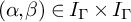
Let $D^-$
and
$D^-$
and $D^+$
be two nonempty, proper, closed and convex subsets of X. A geodesic arc
$D^+$
be two nonempty, proper, closed and convex subsets of X. A geodesic arc ${\widetilde {\rho }}: [0,T]\rightarrow X$
, where
${\widetilde {\rho }}: [0,T]\rightarrow X$
, where $T>0$
,
$T>0$
, ${\widetilde {\rho }}(0)\in D^-$
and
${\widetilde {\rho }}(0)\in D^-$
and ${\widetilde {\rho }}(T)\in D^+$
is a common perpendicular of length
${\widetilde {\rho }}(T)\in D^+$
is a common perpendicular of length $\lambda ({\widetilde {\rho }})=T$
from
$\lambda ({\widetilde {\rho }})=T$
from $D^-$
to
$D^-$
to $D^+$
if its image is the unique shortest geodesic segment from a point of
$D^+$
if its image is the unique shortest geodesic segment from a point of $D^-$
to a point of
$D^-$
to a point of $D^+$
. It exists if and only if the closures
$D^+$
. It exists if and only if the closures $\overline {D^-}$
and
$\overline {D^-}$
and $\overline {D^+}$
of
$\overline {D^+}$
of $D^-$
and
$D^-$
and $D^+$
in
$D^+$
in $X\cup \partial _\infty X$
are disjoint. We refer to [Reference Parkkonen and PaulinPP3], the survey [Reference Parkkonen and PaulinPP2], or [Reference Broise-Alamichel, Parkkonen and PaulinBrPP, §2.5, §12.1 and §12.4] for further details on common perpendiculars.
$X\cup \partial _\infty X$
are disjoint. We refer to [Reference Parkkonen and PaulinPP3], the survey [Reference Parkkonen and PaulinPP2], or [Reference Broise-Alamichel, Parkkonen and PaulinBrPP, §2.5, §12.1 and §12.4] for further details on common perpendiculars.
The following lemma connects strongly reversible loxodromic elements of $\Gamma $
with common perpendiculars between the fixed point sets of involutions. This connection is the key to the proofs of the main results in Sections 5 and 6.
$\Gamma $
with common perpendiculars between the fixed point sets of involutions. This connection is the key to the proofs of the main results in Sections 5 and 6.
Lemma 2.3. Let $(\alpha ,\beta )\in I_\Gamma \times I_\Gamma $
, and let I and J be two
$(\alpha ,\beta )\in I_\Gamma \times I_\Gamma $
, and let I and J be two $\Gamma $
-invariant and nonempty subsets of
$\Gamma $
-invariant and nonempty subsets of $I_\Gamma $
. The product
$I_\Gamma $
. The product $\gamma =\beta \alpha $
is strongly reversible, and it is
$\gamma =\beta \alpha $
is strongly reversible, and it is $\{I,J\}$
-reversible if furthermore
$\{I,J\}$
-reversible if furthermore $\alpha \in I$
and
$\alpha \in I$
and $\beta \in J$
. It is
$\beta \in J$
. It is
-
(i) elliptic or the identity if and only if
$F_\alpha \cap F_\beta \neq \emptyset $
, -
(ii) loxodromic if and only if
$\overline {F_\alpha } \,\cap \,\overline { F_\beta } =\emptyset $
, -
(iii) parabolic if and only if
$F_\alpha \cap F_\beta =\emptyset $
and
$\overline {F_\alpha }\,\cap \,\overline {F_\beta }\neq \emptyset $
.


In cases (ii) and (iii), the group $\langle \alpha ,\beta \rangle $
generated by
$\langle \alpha ,\beta \rangle $
generated by $\alpha $
and
$\alpha $
and $\beta $
is an infinite dihedral group and we have
$\beta $
is an infinite dihedral group and we have
 $$\begin{align*}\langle\alpha,\beta\rangle=\langle\alpha\rangle*\langle\beta\rangle\;. \end{align*}$$
If $\gamma $
is loxodromic, the translation axis
$\gamma $
is loxodromic, the translation axis $\operatorname {Ax}_\gamma $
of
$\operatorname {Ax}_\gamma $
of $\gamma $
is the union of the images by the elements of the group
$\gamma $
is the union of the images by the elements of the group $\langle \alpha , \beta \rangle $
of the common perpendicular segment
$\langle \alpha , \beta \rangle $
of the common perpendicular segment ${\widetilde {\rho }}_{\alpha , \beta }$
from
${\widetilde {\rho }}_{\alpha , \beta }$
from $F_{\alpha }$
to
$F_{\alpha }$
to $F_{\beta }$
, and the translation length of
$F_{\beta }$
, and the translation length of $\gamma $
satisfies
$\gamma $
satisfies
 $$ \begin{align} \lambda(\gamma)=2\;d(F_\alpha,F_\beta)\,. \end{align} $$
Proof. Let $\alpha \in I$
and
$\alpha \in I$
and $\beta \in J$
(with possibly
$\beta \in J$
(with possibly $I=J= I_\Gamma $
). Let
$I=J= I_\Gamma $
). Let $\gamma =\beta \alpha $
. Then
$\gamma =\beta \alpha $
. Then $\alpha $
is a
$\alpha $
is a $\gamma $
-reversing involution for
$\gamma $
-reversing involution for $(I,J)$
, and hence
$(I,J)$
, and hence $\gamma $
is
$\gamma $
is $\{I,J\}$
-reversible, since
$\{I,J\}$
-reversible, since $\gamma \alpha =\beta \in J$
and
$\gamma \alpha =\beta \in J$
and
 $$ \begin{align} \alpha \gamma\alpha^{-1}= \alpha (\beta \alpha ) \alpha^{-1}=\alpha \beta=(\beta \alpha )^{-1}=\gamma^{-1}\,. \end{align} $$
If $F_\alpha \cap F_\beta \neq \emptyset $
, then
$F_\alpha \cap F_\beta \neq \emptyset $
, then $\gamma =\beta \alpha $
pointwise fixes this intersection and
$\gamma =\beta \alpha $
pointwise fixes this intersection and $\gamma $
is elliptic.
$\gamma $
is elliptic.
Assume that $F_\alpha \cap F_\beta =\emptyset $
. If the intersection
$F_\alpha \cap F_\beta =\emptyset $
. If the intersection $\overline {F_\alpha } \,\cap \,\overline {F_\beta }$
is nonempty, then by convexity, this intersection is reduced to a point at infinity
$\overline {F_\alpha } \,\cap \,\overline {F_\beta }$
is nonempty, then by convexity, this intersection is reduced to a point at infinity $\xi \in \partial _\infty X$
, which is fixed by
$\xi \in \partial _\infty X$
, which is fixed by $\alpha $
and
$\alpha $
and $\beta $
, hence by
$\beta $
, hence by $\gamma $
. If X is a tree, then the two convex subsets
$\gamma $
. If X is a tree, then the two convex subsets $F_\alpha $
and
$F_\alpha $
and $F_\beta $
would meet, which has been excluded. Hence X is a manifold. Any horosphere centred at
$F_\beta $
would meet, which has been excluded. Hence X is a manifold. Any horosphere centred at $\xi $
is invariant by
$\xi $
is invariant by $\alpha $
and
$\alpha $
and $\beta $
, hence by
$\beta $
, hence by $\gamma =\beta \alpha $
and by
$\gamma =\beta \alpha $
and by $\gamma ^{-1}= \alpha \beta $
, so that
$\gamma ^{-1}= \alpha \beta $
, so that $\gamma $
is parabolic or elliptic. If a point
$\gamma $
is parabolic or elliptic. If a point $x\in X$
is fixed by
$x\in X$
is fixed by $\beta \alpha $
, then
$\beta \alpha $
, then $\beta $
sends the segment
$\beta $
sends the segment $[x,\alpha x]$
to the segment
$[x,\alpha x]$
to the segment $[\beta x,x]$
, hence it sends the midpoint
$[\beta x,x]$
, hence it sends the midpoint $m_\alpha $
of
$m_\alpha $
of $[x,\alpha x]$
to the midpoint
$[x,\alpha x]$
to the midpoint $m_\beta $
of
$m_\beta $
of $[\beta x,x]$
. But
$[\beta x,x]$
. But $m_\alpha \in F_\alpha $
and
$m_\alpha \in F_\alpha $
and $m_\beta \in F_\beta $
. Hence
$m_\beta \in F_\beta $
. Hence $m_\alpha =\beta ^{-1}m_\beta =m_\beta \in F_\alpha \cap F_\beta $
, contradicting the disjointness of
$m_\alpha =\beta ^{-1}m_\beta =m_\beta \in F_\alpha \cap F_\beta $
, contradicting the disjointness of $F_\alpha $
and
$F_\alpha $
and $F_\beta $
. Thus
$F_\beta $
. Thus $\gamma $
is not elliptic, therefore it is parabolic. In particular,
$\gamma $
is not elliptic, therefore it is parabolic. In particular, $\gamma $
has infinite order, and
$\gamma $
has infinite order, and $\langle \alpha , \beta \rangle $
is indeed isomorphic to
$\langle \alpha , \beta \rangle $
is indeed isomorphic to $\langle \alpha \rangle *\langle \beta \rangle $
.
$\langle \alpha \rangle *\langle \beta \rangle $
.
If $\overline {F_\alpha } \,\cap \,\overline { F_\beta } =\emptyset $
, let
$\overline {F_\alpha } \,\cap \,\overline { F_\beta } =\emptyset $
, let ${\widetilde {\rho }}_{\alpha ,\beta }=[x,y]$
be the common perpendicular from
${\widetilde {\rho }}_{\alpha ,\beta }=[x,y]$
be the common perpendicular from $F_\alpha $
to
$F_\alpha $
to $F_\beta $
(with
$F_\beta $
(with $x\in F_\alpha $
and
$x\in F_\alpha $
and $y\in F_\beta $
, see Figure 3). We claim that
$y\in F_\beta $
, see Figure 3). We claim that $\alpha [y,x]\cup [x,y]$
is a geodesic segment. When X is a manifold, this follows from the properties of the action of
$\alpha [y,x]\cup [x,y]$
is a geodesic segment. When X is a manifold, this follows from the properties of the action of $T_x\alpha $
on
$T_x\alpha $
on $\nu _xF_\alpha $
described in Remark 2.2 (5). When X is a tree, the interior of
$\nu _xF_\alpha $
described in Remark 2.2 (5). When X is a tree, the interior of $[x,y]$
would otherwise contain a fixed point of
$[x,y]$
would otherwise contain a fixed point of $\alpha $
. Similarly,
$\alpha $
. Similarly, $[\alpha y,y]\cup \beta [y,\alpha y]$
is a geodesic segment, and
$[\alpha y,y]\cup \beta [y,\alpha y]$
is a geodesic segment, and $\gamma =\beta \alpha $
maps its first half
$\gamma =\beta \alpha $
maps its first half $[\alpha y,y]$
to its second half
$[\alpha y,y]$
to its second half $[\beta y,\beta \alpha y]$
in an orientation preserving way. This implies that
$[\beta y,\beta \alpha y]$
in an orientation preserving way. This implies that $\gamma $
is loxodromic, that its translation axis contains
$\gamma $
is loxodromic, that its translation axis contains $[\alpha y,y]$
, hence contains
$[\alpha y,y]$
, hence contains ${\widetilde {\rho }}_{\alpha ,\beta }$
, and that
${\widetilde {\rho }}_{\alpha ,\beta }$
, and that
 $$\begin{align*}\lambda(\gamma)=d(\alpha y,y)=2 \,d(x,y)=2\,d(F_\alpha,F_\beta)\,. \end{align*}$$
Taking the image of the common perpendicular segment ${\widetilde {\rho }}_{\alpha ,\beta }$
by
${\widetilde {\rho }}_{\alpha ,\beta }$
by $\alpha $
, and then the images of
$\alpha $
, and then the images of $\alpha {\widetilde {\rho }}_{\alpha ,\beta }\cup {\widetilde {\rho }}_{\alpha ,\beta }$
by the powers of
$\alpha {\widetilde {\rho }}_{\alpha ,\beta }\cup {\widetilde {\rho }}_{\alpha ,\beta }$
by the powers of $\gamma $
, we cover the whole translation axis
$\gamma $
, we cover the whole translation axis $\operatorname {Ax}_\gamma $
. The fact that
$\operatorname {Ax}_\gamma $
. The fact that $\langle \alpha ,\beta \rangle $
is isomorphic to
$\langle \alpha ,\beta \rangle $
is isomorphic to $\langle \alpha \rangle *\langle \beta \rangle $
follows as in the parabolic case.
$\langle \alpha \rangle *\langle \beta \rangle $
follows as in the parabolic case.
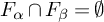
Loxodromic products of two order $2$
elements of
$2$
elements of $\Gamma $
.
$\Gamma $
.

A subgroup H of $\Gamma $
isomorphic to the free product
$\Gamma $
isomorphic to the free product ${\mathbb Z}/2{\mathbb Z}*{\mathbb Z}/2{\mathbb Z}$
of two copies of the cyclic group of order
${\mathbb Z}/2{\mathbb Z}*{\mathbb Z}/2{\mathbb Z}$
of two copies of the cyclic group of order $2$
is an infinite dihedral subgroup of
$2$
is an infinite dihedral subgroup of $\Gamma $
. Note that H is isomorphic to the semidirect product
$\Gamma $
. Note that H is isomorphic to the semidirect product ${\mathbb Z}\rtimes {\mathbb Z}/2{\mathbb Z}$
and it has a canonical morphism onto
${\mathbb Z}\rtimes {\mathbb Z}/2{\mathbb Z}$
and it has a canonical morphism onto ${\mathbb Z}/2{\mathbb Z}$
(mapping any element of order
${\mathbb Z}/2{\mathbb Z}$
(mapping any element of order $2$
to
$2$
to $1\in {\mathbb Z}/2{\mathbb Z}$
), with kernel a canonical infinite cyclic (normal) subgroup
$1\in {\mathbb Z}/2{\mathbb Z}$
), with kernel a canonical infinite cyclic (normal) subgroup $Z_H$
. If
$Z_H$
. If $\alpha \in I$
,
$\alpha \in I$
, $\beta \in J$
and
$\beta \in J$
and $H=\langle \alpha \rangle *\langle \beta \rangle $
, then
$H=\langle \alpha \rangle *\langle \beta \rangle $
, then $\gamma =\beta \alpha $
generates
$\gamma =\beta \alpha $
generates $Z_H$
, and
$Z_H$
, and $\gamma $
is
$\gamma $
is $\{I,J\}$
-reversible in
$\{I,J\}$
-reversible in $\Gamma $
with
$\Gamma $
with $\alpha $
a
$\alpha $
a $\gamma $
-reversing involution for
$\gamma $
-reversing involution for $(I,J)$
by Lemma 2.3.
$(I,J)$
by Lemma 2.3.
We say that an infinite dihedral subgroup H of $\Gamma $
is of loxodromic type if
$\Gamma $
is of loxodromic type if $Z_H$
is generated by a loxodromic element and that it is of parabolic type if
$Z_H$
is generated by a loxodromic element and that it is of parabolic type if $Z_H$
is generated by a parabolic element. Note that when X is a manifold with dimension
$Z_H$
is generated by a parabolic element. Note that when X is a manifold with dimension $2$
and when
$2$
and when $\Gamma $
preserves an orientation, then all infinite dihedral subgroups of
$\Gamma $
preserves an orientation, then all infinite dihedral subgroups of $\Gamma $
are of loxodromic type. In case (ii) of Lemma 2.3, the group
$\Gamma $
are of loxodromic type. In case (ii) of Lemma 2.3, the group $\langle \alpha ,\beta \rangle $
generated by
$\langle \alpha ,\beta \rangle $
generated by $\alpha $
and
$\alpha $
and $\beta $
is an infinite dihedral group of loxodromic type. In case (iii), it is an infinite dihedral group of parabolic type.
$\beta $
is an infinite dihedral group of loxodromic type. In case (iii), it is an infinite dihedral group of parabolic type.
An $\{I,J\}$
-dihedral subgroup of
$\{I,J\}$
-dihedral subgroup of $\Gamma $
is an infinite dihedral subgroup
$\Gamma $
is an infinite dihedral subgroup $\langle \alpha \rangle *\langle \beta \rangle $
of loxodromic type with
$\langle \alpha \rangle *\langle \beta \rangle $
of loxodromic type with $\alpha \in I$
and
$\alpha \in I$
and $\beta \in J$
. We denote by
$\beta \in J$
. We denote by ${\widetilde {\mathfrak D}}_{I,J}$
the set of
${\widetilde {\mathfrak D}}_{I,J}$
the set of $\{I,J\}$
-dihedral subgroups of
$\{I,J\}$
-dihedral subgroups of $\Gamma $
. It is invariant under conjugation by elements of
$\Gamma $
. It is invariant under conjugation by elements of $\Gamma $
.
$\Gamma $
.
Example 2.4. A classical example considered by Sarnak [Reference SarnakSar] is $\Gamma =\operatorname {PSL}_2({\mathbb Z})$
acting by homographies on the upper halfplane model of the real hyperbolic plane
$\Gamma =\operatorname {PSL}_2({\mathbb Z})$
acting by homographies on the upper halfplane model of the real hyperbolic plane ${\widetilde {M}}={{\mathbb H}}^2_{\mathbb R}$
, for which
${\widetilde {M}}={{\mathbb H}}^2_{\mathbb R}$
, for which $I_\Gamma $
is the set
$I_\Gamma $
is the set $I_\alpha $
of conjugates in
$I_\alpha $
of conjugates in $\Gamma $
of
$\Gamma $
of ![]() . As said in the Introduction, Sarnak calls the reversible loxodromic elements of
. As said in the Introduction, Sarnak calls the reversible loxodromic elements of $\operatorname {PSL}_2({\mathbb Z})$
reciprocal. They are strongly reversible by Remark 2.2 (5).
$\operatorname {PSL}_2({\mathbb Z})$
reciprocal. They are strongly reversible by Remark 2.2 (5).
Let $X = {{\mathbb H}}^2_{\mathbb R}$
and let
$X = {{\mathbb H}}^2_{\mathbb R}$
and let $\Gamma $
be the extended modular group, generated by the modular group
$\Gamma $
be the extended modular group, generated by the modular group $\operatorname {PSL}_2({\mathbb Z})$
acting by homographies on
$\operatorname {PSL}_2({\mathbb Z})$
acting by homographies on ${{\mathbb H}}^2_{\mathbb R}$
and by the hyperbolic reflection
${{\mathbb H}}^2_{\mathbb R}$
and by the hyperbolic reflection $\alpha :z\mapsto -\overline {z}$
fixing the vertical geodesic line
$\alpha :z\mapsto -\overline {z}$
fixing the vertical geodesic line $F_\alpha $
with points at infinity
$F_\alpha $
with points at infinity $0,\infty \in \partial _\infty {{\mathbb H}}^2_{\mathbb R}={\mathbb R}\cup \{\infty \}$
. Let
$0,\infty \in \partial _\infty {{\mathbb H}}^2_{\mathbb R}={\mathbb R}\cup \{\infty \}$
. Let $\beta :z \mapsto \frac {-2\,\overline {z}+1}{-3\,\overline {z}+2}\in \Gamma $
, which is the hyperbolic reflection fixing the geodesic line
$\beta :z \mapsto \frac {-2\,\overline {z}+1}{-3\,\overline {z}+2}\in \Gamma $
, which is the hyperbolic reflection fixing the geodesic line $F_{\beta }$
with points at infinity
$F_{\beta }$
with points at infinity $\frac {1}{3}$
and
$\frac {1}{3}$
and $1$
. The composition
$1$
. The composition ![]() is an ambiguous
Footnote 5
loxodromic element of
is an ambiguous
Footnote 5
loxodromic element of $\operatorname {PSL}_2({\mathbb Z})$
. This element
$\operatorname {PSL}_2({\mathbb Z})$
. This element $\gamma$
is
$\gamma$
is $\{I_\alpha ,I_\beta \}$
-reversible since
$\{I_\alpha ,I_\beta \}$
-reversible since $\alpha \in I_\alpha $
conjugates
$\alpha \in I_\alpha $
conjugates $\gamma $
to its inverse
$\gamma $
to its inverse $\gamma ^{-1}=\alpha \beta $
and
$\gamma ^{-1}=\alpha \beta $
and $\beta =\gamma \alpha \in I_\beta $
. But
$\beta =\gamma \alpha \in I_\beta $
. But $\gamma $
is not
$\gamma $
is not $\{I_\alpha , I_\alpha \}$
-reversible, since
$\{I_\alpha , I_\alpha \}$
-reversible, since $\beta =\gamma \alpha $
is not conjugated to
$\beta =\gamma \alpha $
is not conjugated to $\alpha $
in
$\alpha $
in $\Gamma $
, hence does not belong to
$\Gamma $
, hence does not belong to $I_{\alpha }$
. Note that the element
$I_{\alpha }$
. Note that the element ${\gamma ^2= (\beta \alpha \beta ^{-1})\alpha = \beta (\alpha \beta \alpha ^{-1})}$
is
${\gamma ^2= (\beta \alpha \beta ^{-1})\alpha = \beta (\alpha \beta \alpha ^{-1})}$
is $\{I_\alpha , I_\alpha \}$
-reversible and
$\{I_\alpha , I_\alpha \}$
-reversible and $\{I_\beta ,I_\beta \}$
-reversible as said in Remark 2.2 (3). The translation axis of
$\{I_\beta ,I_\beta \}$
-reversible as said in Remark 2.2 (3). The translation axis of $\gamma $
is the geodesic line in
$\gamma $
is the geodesic line in ${{\mathbb H}}^2_{\mathbb R}$
containing the common perpendicular from
${{\mathbb H}}^2_{\mathbb R}$
containing the common perpendicular from $F_\alpha $
to
$F_\alpha $
to $F_\beta $
by Lemma 2.3. See the end of Example 7.4 and [Reference Parkkonen and PaulinPP6, §6] for further details on this example.
$F_\beta $
by Lemma 2.3. See the end of Example 7.4 and [Reference Parkkonen and PaulinPP6, §6] for further details on this example.
We refer to [Reference Broise-Alamichel, Parkkonen and PaulinBrPP, §7.2] for the following definitions concerning equivariant families of (convex) subsets of X. Let $I'$
be an index set endowed with a left action of
$I'$
be an index set endowed with a left action of $\Gamma $
. A family
$\Gamma $
. A family ${\mathcal {D}}=(D_i)_{i\in I'}$
of subsets of X indexed by
${\mathcal {D}}=(D_i)_{i\in I'}$
of subsets of X indexed by $I'$
is
$I'$
is $\Gamma $
-equivariant if
$\Gamma $
-equivariant if $\gamma D_i=D_{\gamma i}$
for all
$\gamma D_i=D_{\gamma i}$
for all $\gamma \in \Gamma $
and
$\gamma \in \Gamma $
and $i\in I'$
. We denote by
$i\in I'$
. We denote by ![]() the equivalence relation on
the equivalence relation on $I'$
defined by
$I'$
defined by ![]() if and only if
if and only if $D_i=D_j$
and there exists
$D_i=D_j$
and there exists $\gamma \in \Gamma $
such that
$\gamma \in \Gamma $
such that $j=\gamma i$
. We say that
$j=\gamma i$
. We say that ${\mathcal {D}}$
is locally finite if for every compact subset K in X, the quotient set
${\mathcal {D}}$
is locally finite if for every compact subset K in X, the quotient set ![]() is finite.
is finite.
The family ${\mathcal {F}}_I=(F_\alpha )_{\alpha \in I}$
is
${\mathcal {F}}_I=(F_\alpha )_{\alpha \in I}$
is $\Gamma $
-equivariant since
$\Gamma $
-equivariant since $\gamma F_\alpha =F_{\gamma \alpha \gamma ^{-1}}$
for all
$\gamma F_\alpha =F_{\gamma \alpha \gamma ^{-1}}$
for all $\gamma \in \Gamma $
and
$\gamma \in \Gamma $
and $\alpha \in I$
, and locally finite by the discreteness of
$\alpha \in I$
, and locally finite by the discreteness of $\Gamma $
. We simplify the notation
$\Gamma $
. We simplify the notation ![]() as
as ![]() , with
, with
When X is a manifold, by Remark 2.1 (2), we have ![]() if and only if
if and only if $\alpha = \beta $
.
$\alpha = \beta $
.
The equivalence relation ![]() on the set I is
on the set I is $\Gamma $
-equivariant: for all
$\Gamma $
-equivariant: for all $\alpha ,\beta \in I$
and
$\alpha ,\beta \in I$
and $\gamma \in \Gamma $
, we have
$\gamma \in \Gamma $
, we have ![]() if and only if
if and only if ![]() . We henceforth endow the quotient set
. We henceforth endow the quotient set ![]() with the quotient left action of the group
with the quotient left action of the group $\Gamma $
.
$\Gamma $
.
For every $\alpha \in I_\Gamma $
, let
$\alpha \in I_\Gamma $
, let $\Gamma _{F_\alpha }=\operatorname {Stab}_\Gamma (F_\alpha )$
be the (global) stabiliser of
$\Gamma _{F_\alpha }=\operatorname {Stab}_\Gamma (F_\alpha )$
be the (global) stabiliser of $F_\alpha $
in
$F_\alpha $
in $\Gamma $
. Let
$\Gamma $
. Let $Z_\Gamma (\alpha )$
be the centraliser of
$Z_\Gamma (\alpha )$
be the centraliser of $\alpha $
in
$\alpha $
in $\Gamma $
, which is contained in
$\Gamma $
, which is contained in $\Gamma _{F_\alpha }$
.
$\Gamma _{F_\alpha }$
.
Lemma 2.5. For every $\gamma \in {\widetilde {\mathfrak R}}_{I,J}$
, the set of pairs
$\gamma \in {\widetilde {\mathfrak R}}_{I,J}$
, the set of pairs $(\alpha ,\beta )\in I\times J$
such that
$(\alpha ,\beta )\in I\times J$
such that $\gamma = \beta \alpha $
is nonempty and invariant under the diagonal left action by conjugation on the product
$\gamma = \beta \alpha $
is nonempty and invariant under the diagonal left action by conjugation on the product $I\times J$
of the centraliser
$I\times J$
of the centraliser $Z_\Gamma (\gamma )$
of
$Z_\Gamma (\gamma )$
of $\gamma $
, and has finite quotient by this action.
$\gamma $
, and has finite quotient by this action.
Proof. Let $\gamma \in {\widetilde {\mathfrak R}}_{I,J}$
. By definition, there exists
$\gamma \in {\widetilde {\mathfrak R}}_{I,J}$
. By definition, there exists $\alpha \in I$
such that
$\alpha \in I$
such that $\beta =\gamma \alpha \in J$
, hence we have
$\beta =\gamma \alpha \in J$
, hence we have $\gamma =\beta \alpha ^{-1}=\beta \alpha $
. For every
$\gamma =\beta \alpha ^{-1}=\beta \alpha $
. For every $\delta \in Z_\Gamma (\gamma )$
, we have
$\delta \in Z_\Gamma (\gamma )$
, we have
 $$\begin{align*}\gamma=\delta\gamma\delta^{-1}= \delta\beta \alpha \delta^{-1}=(\delta\beta\delta^{-1}) (\delta\alpha \delta^{-1})\,, \end{align*}$$
which proves the first claim since I and J are invariant under conjugation.
To prove the second claim, let us fix $x\in \operatorname {Ax}_\gamma $
. Since
$x\in \operatorname {Ax}_\gamma $
. Since $Z_\Gamma (\gamma )$
contains
$Z_\Gamma (\gamma )$
contains $\gamma ^{\mathbb Z}$
which acts on
$\gamma ^{\mathbb Z}$
which acts on $\operatorname {Ax}_\gamma $
with fundamental domain equal to the relatively compact geodesic segment
$\operatorname {Ax}_\gamma $
with fundamental domain equal to the relatively compact geodesic segment $[x,\gamma x[\,$
, up to conjugating
$[x,\gamma x[\,$
, up to conjugating $\alpha $
by an element
$\alpha $
by an element $Z_\Gamma (\gamma )$
, we may assume that the unique fixed point
$Z_\Gamma (\gamma )$
, we may assume that the unique fixed point $f_{\alpha , \gamma }$
of
$f_{\alpha , \gamma }$
of $\alpha $
on
$\alpha $
on $\operatorname {Ax}_\gamma $
belongs to
$\operatorname {Ax}_\gamma $
belongs to $[x,\gamma x]$
. The claim follows since the family
$[x,\gamma x]$
. The claim follows since the family ${\mathcal {F}}_I$
is locally finite.
${\mathcal {F}}_I$
is locally finite.
Lemma 2.6. The group $Z_\Gamma (\alpha )$
has finite index in
$Z_\Gamma (\alpha )$
has finite index in $\Gamma _{F_\alpha }$
. If
$\Gamma _{F_\alpha }$
. If $\alpha \in I$
, the map from
$\alpha \in I$
, the map from $\Gamma _{F_\alpha }/ Z_\Gamma (\alpha )$
to the equivalence class in
$\Gamma _{F_\alpha }/ Z_\Gamma (\alpha )$
to the equivalence class in ![]() of
of $\alpha $
defined by
$\alpha $
defined by $\gamma Z_\Gamma (\alpha )\mapsto \gamma \alpha \gamma ^{-1}$
is a bijection.
$\gamma Z_\Gamma (\alpha )\mapsto \gamma \alpha \gamma ^{-1}$
is a bijection.
Proof. By the discreteness of $\Gamma $
, the point stabilisers of
$\Gamma $
, the point stabilisers of $\Gamma $
in X are finite, hence the equivalence classes of
$\Gamma $
in X are finite, hence the equivalence classes of ![]() are finite. Therefore the first claim follows from the second one. The map from
are finite. Therefore the first claim follows from the second one. The map from $\Gamma /Z_\Gamma (\alpha )$
to the conjugacy class
$\Gamma /Z_\Gamma (\alpha )$
to the conjugacy class $[\alpha ] =\{\gamma \alpha \gamma ^{-1}:\gamma \in \Gamma \}$
of
$[\alpha ] =\{\gamma \alpha \gamma ^{-1}:\gamma \in \Gamma \}$
of $\alpha $
in
$\alpha $
in $\Gamma $
defined by
$\Gamma $
defined by $\gamma Z_\Gamma (\alpha )\mapsto \gamma \alpha \gamma ^{-1}$
is a bijection. For every
$\gamma Z_\Gamma (\alpha )\mapsto \gamma \alpha \gamma ^{-1}$
is a bijection. For every $\gamma \in \Gamma $
, we have
$\gamma \in \Gamma $
, we have $F_{\gamma \alpha \gamma ^{-1}}= F_\alpha $
if and only if
$F_{\gamma \alpha \gamma ^{-1}}= F_\alpha $
if and only if $\gamma \in \Gamma _{F_\alpha }$
. The result follows by the definition of
$\gamma \in \Gamma _{F_\alpha }$
. The result follows by the definition of ![]() .
.
Note that when X is a tree, we can have $|\Gamma _{F_\alpha }/ Z_\Gamma (\alpha )|>1$
, see Lemma 7.9. However, when X is a manifold, we have
$|\Gamma _{F_\alpha }/ Z_\Gamma (\alpha )|>1$
, see Lemma 7.9. However, when X is a manifold, we have $|\Gamma _{F_\alpha }/ Z_\Gamma (\alpha )|=1$
and the equivalence classes for
$|\Gamma _{F_\alpha }/ Z_\Gamma (\alpha )|=1$
and the equivalence classes for ![]() are singletons, see Remark 2.1 (2).
are singletons, see Remark 2.1 (2).
3 Multisets of strongly reversible loxodromic elements
A set with multiplicity or a (positive real valued) multiset is a pair $A=(\underline A,\omega )$
, where
$A=(\underline A,\omega )$
, where $\underline A$
is a set, called the underlying set of A, and
$\underline A$
is a set, called the underlying set of A, and $\omega : \underline A\to \;]0,+\infty [$
is a positive function, called the multiplicity of A. By an element of A, we mean an element of
$\omega : \underline A\to \;]0,+\infty [$
is a positive function, called the multiplicity of A. By an element of A, we mean an element of $\underline A$
. If
$\underline A$
. If $E=(\underline E,\omega )$
and
$E=(\underline E,\omega )$
and $E'= (\underline E',\omega ')$
are multisets, a multiset bijection
$E'= (\underline E',\omega ')$
are multisets, a multiset bijection $f:E\to E'$
is a surjective map
$f:E\to E'$
is a surjective map $f:\underline E\rightarrow \underline E'$
such that for every
$f:\underline E\rightarrow \underline E'$
such that for every $x'\in \underline{E'}$
, we have
$x'\in \underline{E'}$
, we have
 $$ \begin{align*}\omega'(x')= \sum_{x\in f^{-1} (x')} \omega(x)\,.\end{align*} $$
If $E=(\underline E,\omega )$
is a multiset and
$E=(\underline E,\omega )$
is a multiset and $\underline A\subset \underline E$
, the multiset
$\underline A\subset \underline E$
, the multiset $A=(\underline A,\omega |_A)$
is a restriction of E.
$A=(\underline A,\omega |_A)$
is a restriction of E.
As a preparation for the proofs in Sections 5 and 6, we define various multisets associated with strongly reversible loxodromic elements of $\Gamma $
. At the end of this Section, we prove that there are multiset bijections between these multisets.
$\Gamma $
. At the end of this Section, we prove that there are multiset bijections between these multisets.
Let
 $$\begin{align*}{\widetilde{IJ}}=\big\{(\alpha,\beta)\in I\times J : \overline{F_{\alpha}}\,\cap\,\overline{F_{\beta}}\,=\emptyset\big\}\,. \end{align*}$$
Note that $(\alpha ,\beta )\in {\widetilde {IJ}}$
if and only if
$(\alpha ,\beta )\in {\widetilde {IJ}}$
if and only if $(\beta ,\alpha ) \in {\widetilde {JI}}$
. Let
$(\beta ,\alpha ) \in {\widetilde {JI}}$
. Let ![]() be the diagonal equivalence relation on
be the diagonal equivalence relation on $I\times J$
, defined by
$I\times J$
, defined by ![]() if and only if
if and only if ![]() and
and ![]() . The condition
. The condition $\overline {F_{\alpha }}\,\cap \, \overline {F_{\beta }}\, =\emptyset $
for
$\overline {F_{\alpha }}\,\cap \, \overline {F_{\beta }}\, =\emptyset $
for $(\alpha , \beta )\in I\times J$
is constant on the equivalence classes modulo
$(\alpha , \beta )\in I\times J$
is constant on the equivalence classes modulo ![]() and on the orbits of the diagonal left action of the group
and on the orbits of the diagonal left action of the group $\Gamma $
on
$\Gamma $
on $I \times J$
. Hence the subset
$I \times J$
. Hence the subset ${\widetilde {IJ}}$
of
${\widetilde {IJ}}$
of $I\times J$
is saturated by
$I\times J$
is saturated by ![]() and
and $\Gamma $
-invariant.
$\Gamma $
-invariant.
We define the multiset $IJ$
with underlying set
$IJ$
with underlying set $\underline {IJ}= \Gamma \backslash {\widetilde {IJ}}$
and multiplicity given by
$\underline {IJ}= \Gamma \backslash {\widetilde {IJ}}$
and multiplicity given by
 $$ \begin{align} \forall\;\Gamma(\alpha,\beta)\in \underline{IJ},\quad \operatorname{mult}(\Gamma(\alpha,\beta))= \frac{1}{{\operatorname{Card}}(\Gamma_{F_\alpha}\cap\Gamma_{F_\beta})\; |\Gamma_{F_\alpha}/Z_\Gamma(\alpha)|\; |\Gamma_{F_\beta}/Z_\Gamma(\beta)|}\,. \end{align} $$
The right hand side of the above formula for $(\alpha , \beta )\in {\widetilde {IJ}}$
is constant on the equivalence classes modulo
$(\alpha , \beta )\in {\widetilde {IJ}}$
is constant on the equivalence classes modulo ![]() and on the orbits of
and on the orbits of $\Gamma $
on
$\Gamma $
on ${\widetilde {IJ}}$
, hence
${\widetilde {IJ}}$
, hence $\operatorname {mult}(\Gamma (\alpha ,\beta ))$
is well defined.
$\operatorname {mult}(\Gamma (\alpha ,\beta ))$
is well defined.
For every $T>0$
, we define the multiset restriction
$T>0$
, we define the multiset restriction $IJ(T)$
of
$IJ(T)$
of $IJ$
by setting
$IJ$
by setting
 $$ \begin{align} \underline{IJ(T)}= \big\{\Gamma(\alpha,\beta)\in \underline{IJ}:d(F_\alpha,F_\beta)\leq T\}\,. \end{align} $$
We denote by ${\mathfrak R}_{I,J}$
the multiset, whose underlying set is the set
${\mathfrak R}_{I,J}$
the multiset, whose underlying set is the set $\underline {{\mathfrak R}_{I,J}}=\Gamma \backslash {\widetilde {\mathfrak R}}_{I, J}$
of conjugacy classes
$\underline {{\mathfrak R}_{I,J}}=\Gamma \backslash {\widetilde {\mathfrak R}}_{I, J}$
of conjugacy classes $[\gamma ]$
of
$[\gamma ]$
of $\{I,J\}$
-reversible loxodromic elements
$\{I,J\}$
-reversible loxodromic elements $\gamma $
of
$\gamma $
of $\Gamma $
, and where the multiplicity of
$\Gamma $
, and where the multiplicity of $[\gamma ]\in {\mathfrak R}_{I,J}$
is defined by
$[\gamma ]\in {\mathfrak R}_{I,J}$
is defined by
 $$ \begin{align} &\operatorname{mult}([\gamma])= \sum_{\Gamma(\alpha,\,\beta)\,\in\,\underline{IJ}\;:\;\beta\alpha\,\in\,[\gamma]}\; \operatorname{mult}(\Gamma(\alpha,\beta))\,. \end{align} $$
We have ${\mathfrak R}_{I,J}={\mathfrak R}_{J,I}$
. For every
${\mathfrak R}_{I,J}={\mathfrak R}_{J,I}$
. For every $T>0$
, we denote by
$T>0$
, we denote by ${\mathfrak R}_{I,J}(T)$
the multiset restriction of
${\mathfrak R}_{I,J}(T)$
the multiset restriction of ${\mathfrak R}_{I,J}$
to its elements with translation length at most T.
${\mathfrak R}_{I,J}$
to its elements with translation length at most T.
Remark 3.1.
-
(1) Equation (6) is independent of the choices of representatives
$(\alpha , \beta )\in {\widetilde {IJ}}$
in their
$\Gamma $
-orbit, since
$(\gamma '\beta {\gamma '}^{-1})(\gamma '\alpha {\gamma '}^{-1})=\gamma '(\beta \alpha ){\gamma '}^{-1}$
for all
$\gamma '\in \Gamma $
. The sum in Equation (6) has a finite index set by the last assertion of Lemma 2.5. This sum is positive by the first assertion of Lemma 2.5. -
(2) The multiplicity
$\operatorname {mult}([\gamma ])$
depends only on the conjugacy class
$[\gamma ]= [\gamma ^{-1}]$
of the
$\{I,J\}$
-reversible loxodromic element
$\gamma $
in
$\Gamma $
. -
(3) Assume in this remark that
$X={\widetilde {M}}$
is a manifold and that the elliptic elements of
$\Gamma $
only have isolated fixed points. Equivalently, no element of
$\Gamma - \{\operatorname {id}\}$
fixes a nontrivial geodesic segment in X. Thus, for all
$\alpha ,\beta \in I_\Gamma $
with
$\alpha \ne \beta $
, every element of
$\Gamma _{F_\alpha }\cap \Gamma _{F_\beta }$
is trivial, because it fixes pointwise the (nontrivial) common perpendicular between
$F_\alpha $
and
$F_\beta $
. We have
$|\Gamma _{F_\alpha }/Z_\Gamma (\alpha )|=|\Gamma _{F_\beta }/ Z_\Gamma (\beta )| =1$
as seen at the end of Section 2. Hence we have
$$\begin{align*}\operatorname{mult}([\gamma])={\operatorname{Card}}\big\{\Gamma(\alpha,\,\beta)\,\in\,IJ \;:\;[\beta\alpha]=[\gamma]\big\}\,. \end{align*}$$


Here is a particular case when the computation of the multiplicity of the conjugacy class of a strongly reversible loxodromic element of $\Gamma$
is easy. An element
$\Gamma$
is easy. An element $\gamma \in \Gamma $
is primitive if it is not a proper power in
$\gamma \in \Gamma $
is primitive if it is not a proper power in $\Gamma $
. An element
$\Gamma $
. An element $\gamma \in {\widetilde {\mathfrak R}}_{I,J}$
is
$\gamma \in {\widetilde {\mathfrak R}}_{I,J}$
is $\{I,J\}$
-primitive if it is not a proper power of an element of
$\{I,J\}$
-primitive if it is not a proper power of an element of ${\widetilde {\mathfrak R}}_{I,J}$
. This property being invariant under conjugation by
${\widetilde {\mathfrak R}}_{I,J}$
. This property being invariant under conjugation by $\Gamma $
, we also say that the conjugacy class
$\Gamma $
, we also say that the conjugacy class $[\gamma ]\in {\mathfrak R}_{I,J}$
of
$[\gamma ]\in {\mathfrak R}_{I,J}$
of $\gamma $
is
$\gamma $
is $\{I,J\}$
-primitive. We denote the set of conjugacy classes of
$\{I,J\}$
-primitive. We denote the set of conjugacy classes of $\{I,J\}$
-primitive elements in
$\{I,J\}$
-primitive elements in $\Gamma $
by
$\Gamma $
by ${\mathfrak R}_{I,\,J,\,\mathrm {prim}}$
.
${\mathfrak R}_{I,\,J,\,\mathrm {prim}}$
.
Lemma 3.2. Assume that ${\widetilde {M}}$
has dimension
${\widetilde {M}}$
has dimension $2$
, that
$2$
, that $\Gamma $
preserves an orientation of
$\Gamma $
preserves an orientation of ${\widetilde {M}}$
, and that
${\widetilde {M}}$
, and that $I=J=I_\Gamma $
. If
$I=J=I_\Gamma $
. If $\gamma $
is a primitive, strongly reversible and loxodromic element of
$\gamma $
is a primitive, strongly reversible and loxodromic element of $\Gamma $
, then
$\Gamma $
, then
 $$\begin{align*}\operatorname{mult}([\gamma])=2\,. \end{align*}$$
Proof. Let $(\alpha ,\,\beta )$
and
$(\alpha ,\,\beta )$
and $(\alpha ',\,\beta ')$
be two elements of
$(\alpha ',\,\beta ')$
be two elements of ${\widetilde {IJ}}$
such that
${\widetilde {IJ}}$
such that $[\beta \alpha ]=[\beta '\alpha ']=[\gamma ]$
. Up to replacing them by other elements in their
$[\beta \alpha ]=[\beta '\alpha ']=[\gamma ]$
. Up to replacing them by other elements in their $\Gamma $
-orbits in
$\Gamma $
-orbits in ${\widetilde {IJ}}$
, we may assume that
${\widetilde {IJ}}$
, we may assume that $\beta \alpha =\beta '\alpha '=\gamma $
. Let
$\beta \alpha =\beta '\alpha '=\gamma $
. Let $x_\alpha , x_\beta , x_{\alpha '}, x_{\beta '}$
be the (isolated) fixed point of
$x_\alpha , x_\beta , x_{\alpha '}, x_{\beta '}$
be the (isolated) fixed point of $\alpha ,\beta ,\alpha ', \beta '$
respectively. They belong to the translation axis
$\alpha ,\beta ,\alpha ', \beta '$
respectively. They belong to the translation axis $\operatorname {Ax}_\gamma $
of
$\operatorname {Ax}_\gamma $
of $\gamma $
, see Figure 4. Since
$\gamma $
, see Figure 4. Since $[x_\alpha ,\gamma x_\alpha [$
is a fundamental domain for the action of
$[x_\alpha ,\gamma x_\alpha [$
is a fundamental domain for the action of $\gamma ^{\mathbb Z}$
on
$\gamma ^{\mathbb Z}$
on $\operatorname {Ax}_\gamma $
, up to diagonally conjugating
$\operatorname {Ax}_\gamma $
, up to diagonally conjugating $(\alpha ',\beta ')$
by an element of
$(\alpha ',\beta ')$
by an element of $Z_\Gamma (\gamma )$
, we may assume that
$Z_\Gamma (\gamma )$
, we may assume that $x_{\alpha '}\in [x_\alpha , \gamma x_\alpha [\,$
.
$x_{\alpha '}\in [x_\alpha , \gamma x_\alpha [\,$
.
The translation axis of a loxodromic strongly reversible element of $\Gamma $
.
$\Gamma $
.

If $x_{\alpha '}=x_\alpha $
, then since
$x_{\alpha '}=x_\alpha $
, then since ${\widetilde {M}}$
is a manifold, we have
${\widetilde {M}}$
is a manifold, we have $\alpha '=\alpha $
by Remark 2.1 (2). Hence,
$\alpha '=\alpha $
by Remark 2.1 (2). Hence, $\beta '=\beta $
and
$\beta '=\beta $
and $\Gamma (\alpha ,\,\beta )= \Gamma (\alpha ',\,\beta ')$
. Otherwise, we have the following three cases to consider.
$\Gamma (\alpha ,\,\beta )= \Gamma (\alpha ',\,\beta ')$
. Otherwise, we have the following three cases to consider.
If $x_{\alpha '}\in \;]x_\alpha , x_\beta [\,$
, then the element
$x_{\alpha '}\in \;]x_\alpha , x_\beta [\,$
, then the element $\alpha ' \alpha \in \Gamma $
is loxodromic, with same translation axis as
$\alpha ' \alpha \in \Gamma $
is loxodromic, with same translation axis as $\gamma $
, but with translation length
$\gamma $
, but with translation length $\lambda (\alpha ' \alpha) = 2\,d(x_\alpha , x_{\alpha '})<2\,d(x_\alpha ,x_\beta )=\lambda (\gamma )$
, contradicting the fact that
$\lambda (\alpha ' \alpha) = 2\,d(x_\alpha , x_{\alpha '})<2\,d(x_\alpha ,x_\beta )=\lambda (\gamma )$
, contradicting the fact that $\gamma $
is primitive.
$\gamma $
is primitive.
If $x_{\alpha '}\in \;]x_\beta ,\gamma x_\alpha [\,$
, then similarly considering the element
$x_{\alpha '}\in \;]x_\beta ,\gamma x_\alpha [\,$
, then similarly considering the element $\alpha '\beta $
contradicts the fact that
$\alpha '\beta $
contradicts the fact that $\gamma $
is primitive.
$\gamma $
is primitive.
Hence $x_{\alpha '}=x_\beta $
. Therefore
$x_{\alpha '}=x_\beta $
. Therefore $\alpha '=\beta $
, and
$\alpha '=\beta $
, and $x_{\beta '}=\gamma x_\alpha =\beta x_\alpha =x_{\beta \alpha \beta ^{-1}}$
, so that we have
$x_{\beta '}=\gamma x_\alpha =\beta x_\alpha =x_{\beta \alpha \beta ^{-1}}$
, so that we have $\beta '=\beta \alpha \beta ^{-1}$
, and there is only one possibility that
$\beta '=\beta \alpha \beta ^{-1}$
, and there is only one possibility that $\Gamma (\alpha ',\, \beta ')= \Gamma (\beta ,\alpha )$
. Note that we have
$\Gamma (\alpha ',\, \beta ')= \Gamma (\beta ,\alpha )$
. Note that we have $\Gamma (\alpha ,\,\beta )\neq \Gamma (\beta ,\,\alpha )$
: Otherwise there exists
$\Gamma (\alpha ,\,\beta )\neq \Gamma (\beta ,\,\alpha )$
: Otherwise there exists $\delta \in \Gamma $
so that
$\delta \in \Gamma $
so that $\beta =\delta \alpha \delta ^{-1}$
and
$\beta =\delta \alpha \delta ^{-1}$
and $\alpha = \delta \beta \delta ^{-1}$
. But then
$\alpha = \delta \beta \delta ^{-1}$
. But then $\delta x_\alpha =x_\beta $
and
$\delta x_\alpha =x_\beta $
and $\delta x_\beta =x_\alpha $
, so that
$\delta x_\beta =x_\alpha $
, so that $\delta $
fixes the midpoint of the geodesic segment
$\delta $
fixes the midpoint of the geodesic segment $[x_\alpha , x_\beta ]$
. Considering the element
$[x_\alpha , x_\beta ]$
. Considering the element $\delta \alpha $
again contradicts the fact that
$\delta \alpha $
again contradicts the fact that $\gamma $
is primitive. This proves the result.
$\gamma $
is primitive. This proves the result.
A common perpendicular $\rho $
of type
$\rho $
of type $(I,J)$
is the
$(I,J)$
is the $\Gamma $
-orbit of the common perpendicular
$\Gamma $
-orbit of the common perpendicular ${\widetilde {\rho }}_{\alpha ,\beta }$
from
${\widetilde {\rho }}_{\alpha ,\beta }$
from $F_{\alpha }$
to
$F_{\alpha }$
to $F_{\beta }$
, where
$F_{\beta }$
, where $(\alpha , \beta )$
ranges over
$(\alpha , \beta )$
ranges over ${\widetilde {IJ}}$
. Note that
${\widetilde {IJ}}$
. Note that
 $$ \begin{align} \text{and}\qquad \forall\,(\alpha,\beta)\in {\widetilde{IJ}},\quad\forall\;\gamma\in\Gamma,\qquad \gamma \;{\widetilde{\rho}}_{\alpha,\beta} ={\widetilde{\rho}}_{\gamma\alpha\gamma^{-1},\gamma\beta\gamma^{-1}} \,. \end{align} $$
We then denote ![]() , where
, where ![]() is defined in Section 4. We remark that such a pair
is defined in Section 4. We remark that such a pair $(\alpha , \beta )$
is not necessarily unique. The length
$(\alpha , \beta )$
is not necessarily unique. The length $\lambda (\rho )$
of
$\lambda (\rho )$
of $\rho $
is the length of any such
$\rho $
is the length of any such ${\widetilde {\rho }}_{\alpha , \beta }$
. The multiplicity of
${\widetilde {\rho }}_{\alpha , \beta }$
. The multiplicity of $\rho $
is
$\rho $
is
 $$ \begin{align} \operatorname{mult}(\rho) =\sum_{\Gamma(\alpha,\,\beta)\,\in\, \underline{IJ}, \;\;\rho= \rho_{\alpha,\beta}} \frac{1}{{\operatorname{Card}}(\Gamma_{F_\alpha}\cap\Gamma_{F_\beta})\; |\Gamma_{F_\alpha}/Z_\Gamma(\alpha)|\; |\Gamma_{F_\beta}/Z_\Gamma(\beta)|}\,. \end{align} $$
This sum does not depend on the choice of a representative $(\alpha , \beta )$
in each orbit of
$(\alpha , \beta )$
in each orbit of $\Gamma $
in
$\Gamma $
in ${\widetilde {IJ}}$
, and is finite by the local finiteness of the families
${\widetilde {IJ}}$
, and is finite by the local finiteness of the families ${\mathcal {F}}_I$
and
${\mathcal {F}}_I$
and ${\mathcal {F}}_J$
. Recall that if
${\mathcal {F}}_J$
. Recall that if $(\alpha ,\beta )\in {\widetilde {IJ}}$
, then
$(\alpha ,\beta )\in {\widetilde {IJ}}$
, then $(\beta ,\alpha )\in {\widetilde {JI}}$
, and note that
$(\beta ,\alpha )\in {\widetilde {JI}}$
, and note that
 $$ \begin{align} \operatorname{mult}(\rho_{\alpha,\beta})=\operatorname{mult}(\rho_{\beta,\alpha})\,. \end{align} $$
We denote by $\operatorname {Perp}({\mathcal {F}}_I,{\mathcal {F}}_J)$
the multiset of the common perpendiculars of type
$\operatorname {Perp}({\mathcal {F}}_I,{\mathcal {F}}_J)$
the multiset of the common perpendiculars of type $(I,J)$
. For every
$(I,J)$
. For every $T>0$
, we denote by
$T>0$
, we denote by $\operatorname {Perp} ({\mathcal {F}}_I,{\mathcal {F}}_J,T)$
the multiset restriction of
$\operatorname {Perp} ({\mathcal {F}}_I,{\mathcal {F}}_J,T)$
the multiset restriction of $\operatorname {Perp}({\mathcal {F}}_I,{\mathcal {F}}_J)$
to its elements with length at most T and by
$\operatorname {Perp}({\mathcal {F}}_I,{\mathcal {F}}_J)$
to its elements with length at most T and by $\underline {\operatorname {Perp}} ({\mathcal {F}}_I,{\mathcal {F}}_J,T)$
its underlying set.
$\underline {\operatorname {Perp}} ({\mathcal {F}}_I,{\mathcal {F}}_J,T)$
its underlying set.
Proposition 3.3. There exist two multiset bijections $\Theta _1: IJ\to \operatorname {Perp}({\mathcal {F}}_I,{\mathcal {F}}_J)$
and
$\Theta _1: IJ\to \operatorname {Perp}({\mathcal {F}}_I,{\mathcal {F}}_J)$
and $\Theta _2: IJ\to {\mathfrak R}_{I,J}$
such that for every
$\Theta _2: IJ\to {\mathfrak R}_{I,J}$
such that for every $(\alpha ,\beta )\in {\widetilde {IJ}}$
, we have
$(\alpha ,\beta )\in {\widetilde {IJ}}$
, we have
 $$\begin{align*}\Theta_1(\Gamma (\alpha,\beta)) = \rho_{\alpha,\beta} \quad\text{and}\quad\Theta_2(\Gamma(\alpha,\beta))=[\beta\alpha]\,. \end{align*}$$
Furthermore, for every $T>0$
, the maps
$T>0$
, the maps $\Theta _1$
and
$\Theta _1$
and $\Theta _2$
send
$\Theta _2$
send $IJ(T)$
to
$IJ(T)$
to $\operatorname {Perp}({\mathcal {F}}_I,{\mathcal {F}}_J,T)$
and
$\operatorname {Perp}({\mathcal {F}}_I,{\mathcal {F}}_J,T)$
and ${\mathfrak R}_{I,J}(2T)$
respectively.
${\mathfrak R}_{I,J}(2T)$
respectively.
Proof. The map $\Theta _1: \underline {IJ}=\Gamma \backslash {\widetilde {IJ}}\to \underline {\operatorname {Perp}}({\mathcal {F}}_I,{\mathcal {F}}_J)$
defined by
$\Theta _1: \underline {IJ}=\Gamma \backslash {\widetilde {IJ}}\to \underline {\operatorname {Perp}}({\mathcal {F}}_I,{\mathcal {F}}_J)$
defined by $\Gamma (\alpha ,\beta )\mapsto \rho _{\alpha ,\beta }=\Gamma {\widetilde {\rho }}_{\alpha ,\beta }$
is well-defined by Equation (8) and is surjective by the definition of a common perpendicular of type
$\Gamma (\alpha ,\beta )\mapsto \rho _{\alpha ,\beta }=\Gamma {\widetilde {\rho }}_{\alpha ,\beta }$
is well-defined by Equation (8) and is surjective by the definition of a common perpendicular of type $(I,J)$
. By Equations (9) and (4), for every element
$(I,J)$
. By Equations (9) and (4), for every element $\rho \in \operatorname {Perp}({\mathcal {F}}_I,{\mathcal {F}}_J)$
, we have
$\rho \in \operatorname {Perp}({\mathcal {F}}_I,{\mathcal {F}}_J)$
, we have $\operatorname {mult}(\rho ) = \sum _{\Gamma (\alpha ,\,\beta )\,\in \,\Theta _1^{-1}(\rho )}\operatorname {mult}(\alpha ,\beta )$
. Hence
$\operatorname {mult}(\rho ) = \sum _{\Gamma (\alpha ,\,\beta )\,\in \,\Theta _1^{-1}(\rho )}\operatorname {mult}(\alpha ,\beta )$
. Hence $\Theta _1$
is a multiset bijection from
$\Theta _1$
is a multiset bijection from $IJ$
to
$IJ$
to $\operatorname {Perp}({\mathcal {F}}_I,{\mathcal {F}}_J)$
.
$\operatorname {Perp}({\mathcal {F}}_I,{\mathcal {F}}_J)$
.
The map ${\widetilde {\Theta }}_2:{\widetilde {IJ}}\to {\widetilde {\mathfrak R}}_{I,J}$
defined by
${\widetilde {\Theta }}_2:{\widetilde {IJ}}\to {\widetilde {\mathfrak R}}_{I,J}$
defined by
 $$\begin{align*}{\widetilde{\Theta}}_2:(\alpha ,\beta )\mapsto\beta \alpha \end{align*}$$
indeed has values in the set ${\widetilde {\mathfrak R}}_{I,J}$
of
${\widetilde {\mathfrak R}}_{I,J}$
of $\{I,J\}$
-reversible loxodromic elements of
$\{I,J\}$
-reversible loxodromic elements of $\Gamma $
by Lemma 2.3. The map
$\Gamma $
by Lemma 2.3. The map ${\widetilde {\Theta }}_2$
is equivariant for the left actions of
${\widetilde {\Theta }}_2$
is equivariant for the left actions of $\Gamma $
by diagonal conjugation on
$\Gamma $
by diagonal conjugation on ${\widetilde {IJ}}$
and by conjugation on
${\widetilde {IJ}}$
and by conjugation on ${\widetilde {\mathfrak R}}_{I,J}$
. The map
${\widetilde {\mathfrak R}}_{I,J}$
. The map ${\widetilde {\Theta }}_2$
is surjective by Lemma 2.5. Hence
${\widetilde {\Theta }}_2$
is surjective by Lemma 2.5. Hence ${\widetilde {\Theta }}_2$
induces a surjective quotient map
${\widetilde {\Theta }}_2$
induces a surjective quotient map $\Theta _2: \underline {IJ} \rightarrow \underline {{\mathfrak R}_{I,J}}$
defined by
$\Theta _2: \underline {IJ} \rightarrow \underline {{\mathfrak R}_{I,J}}$
defined by $\Gamma (\alpha ,\beta )\mapsto [\beta \alpha ]$
. By Equation (6), we have
$\Gamma (\alpha ,\beta )\mapsto [\beta \alpha ]$
. By Equation (6), we have $\operatorname {mult}([\gamma ])= \sum _{\Gamma (\alpha ,\,\beta )\,\in \,(\Theta _2)^{-1}([\gamma ])} \operatorname {mult}\Gamma (\alpha , \beta )$
. Hence
$\operatorname {mult}([\gamma ])= \sum _{\Gamma (\alpha ,\,\beta )\,\in \,(\Theta _2)^{-1}([\gamma ])} \operatorname {mult}\Gamma (\alpha , \beta )$
. Hence $\Theta _2$
is a multiset bijection from
$\Theta _2$
is a multiset bijection from $IJ$
to
$IJ$
to ${\mathfrak R}_{I,J}$
.
${\mathfrak R}_{I,J}$
.
For all $(\alpha ,\beta )\in {\widetilde {IJ}}$
and
$(\alpha ,\beta )\in {\widetilde {IJ}}$
and $T>0$
, the common perpendicular
$T>0$
, the common perpendicular ${\widetilde {\rho }}_{\alpha ,\beta }$
from
${\widetilde {\rho }}_{\alpha ,\beta }$
from $F_{\alpha }$
to
$F_{\alpha }$
to $F_{\beta }$
has length
$F_{\beta }$
has length $\lambda (\rho _{\alpha ,\beta })=d(F_\alpha , F_\beta )$
at most T if and only if the
$\lambda (\rho _{\alpha ,\beta })=d(F_\alpha , F_\beta )$
at most T if and only if the $\{I,J\}$
-reversible loxodromic element
$\{I,J\}$
-reversible loxodromic element $\beta \alpha $
has translation length at most
$\beta \alpha $
has translation length at most $2T$
, by Equation (1). This proves the last claim of Proposition 3.3.
$2T$
, by Equation (1). This proves the last claim of Proposition 3.3.
For every $\{I,J\}$
-dihedral subgroup H of
$\{I,J\}$
-dihedral subgroup H of $\Gamma $
, if
$\Gamma $
, if $\gamma $
generates the infinite cyclic group
$\gamma $
generates the infinite cyclic group $Z_H$
, we define the multiplicity of H as
$Z_H$
, we define the multiplicity of H as
 $$ \begin{align} \operatorname{mult}(H)=\operatorname{mult}([\gamma])\,. \end{align} $$
This multiplicity does not depend on the choice of one of the two generators $\gamma $
of
$\gamma $
of $Z_H$
since
$Z_H$
since $[\gamma ]=[\gamma ^{-1}]$
and it is constant on the conjugacy class of H. We denote by
$[\gamma ]=[\gamma ^{-1}]$
and it is constant on the conjugacy class of H. We denote by ${\mathfrak D}_{I,J}$
the multiset of conjugacy classes in
${\mathfrak D}_{I,J}$
the multiset of conjugacy classes in $\Gamma $
of
$\Gamma $
of $\{I,J\}$
-dihedral subgroups of
$\{I,J\}$
-dihedral subgroups of $\Gamma $
, whose underlying set is
$\Gamma $
, whose underlying set is $\Gamma \backslash {\widetilde {\mathfrak D}}_{I,J}$
(see the paragraph before Example 2.4).
$\Gamma \backslash {\widetilde {\mathfrak D}}_{I,J}$
(see the paragraph before Example 2.4).
Proposition 3.4. The map ${\widetilde {\Theta }}_3$
from
${\widetilde {\Theta }}_3$
from ${\widetilde {\mathfrak D}}_{I,J}$
to
${\widetilde {\mathfrak D}}_{I,J}$
to ${\mathfrak R}_{I,J}$
which associates to
${\mathfrak R}_{I,J}$
which associates to $H\in {\widetilde {\mathfrak D}}_{I,J}$
the conjugacy class of a generator of
$H\in {\widetilde {\mathfrak D}}_{I,J}$
the conjugacy class of a generator of $Z_H$
induces a multiset bijection
$Z_H$
induces a multiset bijection $\Theta _3$
from the multiset
$\Theta _3$
from the multiset ${\mathfrak D}_{I,J}$
to the multiset
${\mathfrak D}_{I,J}$
to the multiset ${\mathfrak R}_{I,J}$
.
${\mathfrak R}_{I,J}$
.
Proof. We have already seen that for every $H\in {\widetilde {\mathfrak D}}_{I,J}$
, any generator of
$H\in {\widetilde {\mathfrak D}}_{I,J}$
, any generator of $Z_H$
is
$Z_H$
is $\{I,J\}$
-reversible and hence, so is its inverse. Thus the map
$\{I,J\}$
-reversible and hence, so is its inverse. Thus the map ${\widetilde {\Theta }}_3$
is well defined. It is surjective by Lemmas 2.5 and 2.3. It is invariant by conjugation since
${\widetilde {\Theta }}_3$
is well defined. It is surjective by Lemmas 2.5 and 2.3. It is invariant by conjugation since $Z_{\gamma 'H{\gamma '}^{-1}}= \gamma 'Z_H{\gamma '}^{-1}$
for all
$Z_{\gamma 'H{\gamma '}^{-1}}= \gamma 'Z_H{\gamma '}^{-1}$
for all $\gamma '\in \Gamma $
and
$\gamma '\in \Gamma $
and $H\in {\widetilde {\mathfrak D}}_{I,J}$
. The definition of the multiplicities in Equation (11) proves that the induced map between the sets with multiplicities
$H\in {\widetilde {\mathfrak D}}_{I,J}$
. The definition of the multiplicities in Equation (11) proves that the induced map between the sets with multiplicities ${\mathfrak D}_{I,J}$
and
${\mathfrak D}_{I,J}$
and ${\mathfrak R}_{I,J}$
is a multiset bijection.
${\mathfrak R}_{I,J}$
is a multiset bijection.
The map $\Theta _3$
restricts to a multiset bijection between the multiset of conjugacy classes of maximalFootnote 6
$\Theta _3$
restricts to a multiset bijection between the multiset of conjugacy classes of maximalFootnote 6 $\{I,J\}$
-dihedral subgroups of loxodromic type and the multiset
$\{I,J\}$
-dihedral subgroups of loxodromic type and the multiset ${\mathfrak R}_{I,\,J,\,\mathrm {prim}}$
of conjugacy classes of
${\mathfrak R}_{I,\,J,\,\mathrm {prim}}$
of conjugacy classes of $\{I,J\}$
-primitive,
$\{I,J\}$
-primitive, $\{I,J\}$
-reversible and loxodromic elements of
$\{I,J\}$
-reversible and loxodromic elements of $\Gamma $
.
$\Gamma $
.
4 Dynamics of the geodesic flow
This whole section consists of background information from [Reference Paulin, Pollicott and SchapiraPPS, Chap. 3, 6, 7] and [Reference Broise-Alamichel, Parkkonen and PaulinBrPP, Chap. 3, 4], to which we refer for proofs, details and complements, in particular for the definitions of the measures generalising the ones given in the introduction.
Geodesics and the geodesic flow. Let $(X,\Gamma )$
be as in the beginning of Section 2. Let
$(X,\Gamma )$
be as in the beginning of Section 2. Let ${\mathcal {G}} X$
be the metric space of all geodesic lines
${\mathcal {G}} X$
be the metric space of all geodesic lines $\ell : {\mathbb R}\rightarrow X$
in X, such that, when X is a tree,
$\ell : {\mathbb R}\rightarrow X$
in X, such that, when X is a tree, $\ell (0)$
is a vertex of
$\ell (0)$
is a vertex of ${\mathbb X}$
. The distance between two elements
${\mathbb X}$
. The distance between two elements $\ell $
and
$\ell $
and $\ell '$
in
$\ell '$
in ${\mathcal {G}} X$
is
${\mathcal {G}} X$
is
 $$ \begin{align} d(\ell,\ell')= \int_{-\infty}^{\infty} d(\ell(t),\ell'(t))\;e^{-2\,|t|}\;dt\,. \end{align} $$
When $X={\widetilde {M}}$
is a manifold, we identify the unit tangent bundle
$X={\widetilde {M}}$
is a manifold, we identify the unit tangent bundle $T^1{\widetilde {M}}$
with
$T^1{\widetilde {M}}$
with ${\mathcal {G}} X$
by the map that associates to a unit tangent vector
${\mathcal {G}} X$
by the map that associates to a unit tangent vector $v\in T^1{\widetilde {M}}$
the unique geodesic line
$v\in T^1{\widetilde {M}}$
the unique geodesic line $\ell \in {\mathcal {G}} X$
whose tangent vector
$\ell \in {\mathcal {G}} X$
whose tangent vector $\dot \ell (0)$
at time
$\dot \ell (0)$
at time $0$
is v. When
$0$
is v. When $T^1{\widetilde {M}}$
is endowed with Sasaki’s metric, this mapping is an
$T^1{\widetilde {M}}$
is endowed with Sasaki’s metric, this mapping is an $\operatorname {Isom}({\widetilde {M}})$
-equivariant bi-Hölder-continuous homeomorphism, see [Reference Broise-Alamichel, Parkkonen and PaulinBrPP, §3.1]. We denote by
$\operatorname {Isom}({\widetilde {M}})$
-equivariant bi-Hölder-continuous homeomorphism, see [Reference Broise-Alamichel, Parkkonen and PaulinBrPP, §3.1]. We denote by $\iota : {\mathcal {G}} X\rightarrow {\mathcal {G}} X$
the involutive time-reversal map
$\iota : {\mathcal {G}} X\rightarrow {\mathcal {G}} X$
the involutive time-reversal map $\ell \mapsto \{t\mapsto \ell (-t)\}$
, and again by
$\ell \mapsto \{t\mapsto \ell (-t)\}$
, and again by $\iota $
the induced map from the phase space
$\iota $
the induced map from the phase space $\Gamma \backslash {\mathcal {G}} X$
to itself. The geodesic flow on
$\Gamma \backslash {\mathcal {G}} X$
to itself. The geodesic flow on ${\mathcal {G}} X$
is the
${\mathcal {G}} X$
is the $\operatorname {Isom}(X)$
-equivariant one-parameter group of homeomorphisms
$\operatorname {Isom}(X)$
-equivariant one-parameter group of homeomorphisms
 $$\begin{align*}{\mathtt{g}^{t}} :\ell\mapsto \{s \mapsto \ell(s+t)\} \end{align*}$$
for all $\ell \in {\mathcal {G}} X$
, with continuous time parameter
$\ell \in {\mathcal {G}} X$
, with continuous time parameter $t\in {\mathbb R}$
if X is a manifold, and discrete time parameter
$t\in {\mathbb R}$
if X is a manifold, and discrete time parameter $t\in {\mathbb Z}$
if X is a tree. We also denote by
$t\in {\mathbb Z}$
if X is a tree. We also denote by $({\mathtt {g}^{t}})_t$
the quotient flow on
$({\mathtt {g}^{t}})_t$
the quotient flow on $\Gamma \backslash {\mathcal {G}} X$
, and call it the geodesic flow on
$\Gamma \backslash {\mathcal {G}} X$
, and call it the geodesic flow on $\Gamma \backslash {\mathcal {G}} X$
.
$\Gamma \backslash {\mathcal {G}} X$
.
A $1$
-Lipschitz map
$1$
-Lipschitz map $w:{\mathbb R}\to X$
which is isometric on a closed interval and has a constant value on each complementary component is a generalised geodesic. If X is a tree, we furthermore require that
$w:{\mathbb R}\to X$
which is isometric on a closed interval and has a constant value on each complementary component is a generalised geodesic. If X is a tree, we furthermore require that $w(0)$
and the constant values on the above-mentioned complementary components are vertices of
$w(0)$
and the constant values on the above-mentioned complementary components are vertices of ${\mathbb X}$
. We denote the Bartels-Lück metric space of generalised geodesics by
${\mathbb X}$
. We denote the Bartels-Lück metric space of generalised geodesics by ![]() , with the metric given by Equation (12), see [Reference Bartels and LückBaL] and [Reference Broise-Alamichel, Parkkonen and PaulinBrPP, §2.2]. The space
, with the metric given by Equation (12), see [Reference Bartels and LückBaL] and [Reference Broise-Alamichel, Parkkonen and PaulinBrPP, §2.2]. The space ![]() isometrically contains
isometrically contains ${\mathcal {G}} X$
. The natural action of
${\mathcal {G}} X$
. The natural action of $\operatorname {Isom}(X)$
on
$\operatorname {Isom}(X)$
on ![]() is isometric. The geodesic flow on
is isometric. The geodesic flow on ${\mathcal {G}} X$
extends by the same formula to a flow on
${\mathcal {G}} X$
extends by the same formula to a flow on ![]() , that we also call the geodesic flow on
, that we also call the geodesic flow on ![]() , and we use the same notation
, and we use the same notation $({\mathtt {g}^{t}})_t$
for it.
$({\mathtt {g}^{t}})_t$
for it.
We consider a common perpendicular (with endpoints in $V\mathbb{X}$
when X is a tree) between two nonempty convex subsets of X of length T as a generalised geodesic in
$V\mathbb{X}$
when X is a tree) between two nonempty convex subsets of X of length T as a generalised geodesic in ![]() , being constant on
, being constant on $]-\infty ,0]$
and
$]-\infty ,0]$
and $[T,+\infty [\,$
.
$[T,+\infty [\,$
.
Potentials. We now introduce the supplementary data (with origin in physics) of potentials on X. Assume first that $X={\widetilde {M}}$
is a manifold. Let
$X={\widetilde {M}}$
is a manifold. Let ${\widetilde {P}}:{\mathcal {G}} X=T^1{\widetilde {M}}\rightarrow {\mathbb R}$
be a potential on X, that is, a
${\widetilde {P}}:{\mathcal {G}} X=T^1{\widetilde {M}}\rightarrow {\mathbb R}$
be a potential on X, that is, a $\Gamma $
-invariant, boundedFootnote 7
and Hölder-continuous real map on
$\Gamma $
-invariant, boundedFootnote 7
and Hölder-continuous real map on $T^1{\widetilde {M}}$
. A potential
$T^1{\widetilde {M}}$
. A potential ${\widetilde {P}}$
is time-reversible if
${\widetilde {P}}$
is time-reversible if ${\widetilde {P}}={\widetilde {P}}\circ \iota $
, where
${\widetilde {P}}={\widetilde {P}}\circ \iota $
, where $\iota $
is the time-reversal map. For all
$\iota $
is the time-reversal map. For all $x,y\in {\widetilde {M}}$
, let us define the amplitude
$x,y\in {\widetilde {M}}$
, let us define the amplitude $\int _x^y{\widetilde {P}}$
of
$\int _x^y{\widetilde {P}}$
of ${\widetilde {P}}$
between x and y to be
${\widetilde {P}}$
between x and y to be $\int _x^y{\widetilde {P}}=0$
if
$\int _x^y{\widetilde {P}}=0$
if $x=y$
and otherwise
$x=y$
and otherwise $\int _x^y{\widetilde {P}}= \int _{0}^{d(x,y)} {\widetilde {P}}({\mathtt {g}^{t}} v) \;dt$
where v is the tangent vector at x to the geodesic segment from x to y.
$\int _x^y{\widetilde {P}}= \int _{0}^{d(x,y)} {\widetilde {P}}({\mathtt {g}^{t}} v) \;dt$
where v is the tangent vector at x to the geodesic segment from x to y.
Now assume that X is a tree, with the notation of the beginning of Section 2. Denote by $V{\mathbb X}$
,
$V{\mathbb X}$
, $E{\mathbb X}$
the sets of vertices and edges of
$E{\mathbb X}$
the sets of vertices and edges of ${\mathbb X}$
, and by
${\mathbb X}$
, and by ${\overline e}$
the opposite edge of an edge e. Let
${\overline e}$
the opposite edge of an edge e. Let ${\widetilde {c}}: E{\mathbb X}\rightarrow {\mathbb R}$
be a (logarithmic) system of conductances (see for instance [Reference ZemanianZem]), that is, a
${\widetilde {c}}: E{\mathbb X}\rightarrow {\mathbb R}$
be a (logarithmic) system of conductances (see for instance [Reference ZemanianZem]), that is, a $\Gamma $
-invariant, bounded real map on
$\Gamma $
-invariant, bounded real map on $E{\mathbb X}$
. For every geodesic line
$E{\mathbb X}$
. For every geodesic line $\ell \in {\mathcal {G}} X$
, we denote by
$\ell \in {\mathcal {G}} X$
, we denote by $e^+_0(\ell )=\ell ([0,1])\in E{\mathbb X}$
the first edge followed by
$e^+_0(\ell )=\ell ([0,1])\in E{\mathbb X}$
the first edge followed by $\ell $
. We define the potential
$\ell $
. We define the potential ${\widetilde {P}}:{\mathcal {G}} X\rightarrow {\mathbb R}$
on X associated with
${\widetilde {P}}:{\mathcal {G}} X\rightarrow {\mathbb R}$
on X associated with ${\widetilde {c}}$
as the map
${\widetilde {c}}$
as the map $\ell \mapsto {\widetilde {c}}\,(e^+_0(\ell ))$
. The potential
$\ell \mapsto {\widetilde {c}}\,(e^+_0(\ell ))$
. The potential ${\widetilde {P}}$
is time-reversible if
${\widetilde {P}}$
is time-reversible if ${\widetilde {c}}(\overline {e})={\widetilde {c}}(e)$
for every
${\widetilde {c}}(\overline {e})={\widetilde {c}}(e)$
for every $e\in E{\mathbb X}$
. For all
$e\in E{\mathbb X}$
. For all $x,y\in V{\mathbb X}$
, let
$x,y\in V{\mathbb X}$
, let $(e_1,e_2, \dots , e_k)$
be the geodesic edge path in
$(e_1,e_2, \dots , e_k)$
be the geodesic edge path in ${\mathbb X}$
between x and y, where
${\mathbb X}$
between x and y, where $k\in {\mathbb N}$
satisfies
$k\in {\mathbb N}$
satisfies $k=0$
if and only if
$k=0$
if and only if $x=y$
. We define the amplitude of
$x=y$
. We define the amplitude of ${\widetilde {P}}$
between x and y to be
${\widetilde {P}}$
between x and y to be $\int _x^y{\widetilde {P}}= \sum _{i=1}^{k} \;\;{\widetilde {c}}\,(e_i)$
.
$\int _x^y{\widetilde {P}}= \sum _{i=1}^{k} \;\;{\widetilde {c}}\,(e_i)$
.
If a potential ${\widetilde {P}}$
is time-reversible, then for all
${\widetilde {P}}$
is time-reversible, then for all $x,y\in {\widetilde {M}}$
or
$x,y\in {\widetilde {M}}$
or $x,y\in V{\mathbb X}$
, we have
$x,y\in V{\mathbb X}$
, we have
 $$ \begin{align} \int_y^x{\widetilde{P}} =\int_x^y{\widetilde{P}}\circ\iota=\int_x^y{\widetilde{P}}\,. \end{align} $$
We denote by $P:\Gamma \backslash {\mathcal {G}} X\rightarrow {\mathbb R}$
the quotient map of
$P:\Gamma \backslash {\mathcal {G}} X\rightarrow {\mathbb R}$
the quotient map of ${\widetilde {P}}$
, that we call a potential on
${\widetilde {P}}$
, that we call a potential on $\Gamma \backslash {\mathcal {G}} X$
.
$\Gamma \backslash {\mathcal {G}} X$
.
Recall that every conjugacy class $[\gamma ]$
of loxodromic elements of
$[\gamma ]$
of loxodromic elements of $\Gamma $
defines a (not necessarily primitive) periodic orbit
$\Gamma $
defines a (not necessarily primitive) periodic orbit ${\mathcal {O}}_{[\gamma ]}$
for the geodesic flow
${\mathcal {O}}_{[\gamma ]}$
for the geodesic flow $({\mathtt {g}^{t}})_t$
on
$({\mathtt {g}^{t}})_t$
on $\Gamma \backslash {\mathcal {G}} X$
, with (not necessary minimal) length
$\Gamma \backslash {\mathcal {G}} X$
, with (not necessary minimal) length $\lambda ({\mathcal {O}}_{[\gamma ]}) = \lambda (\gamma )$
, so that for every
$\lambda ({\mathcal {O}}_{[\gamma ]}) = \lambda (\gamma )$
, so that for every $\ell \in {\mathcal {G}} X$
with
$\ell \in {\mathcal {G}} X$
with $\Gamma \ell \in {\mathcal {O}}_{[\gamma ]}$
, there exists a conjugate
$\Gamma \ell \in {\mathcal {O}}_{[\gamma ]}$
, there exists a conjugate $\gamma '$
of
$\gamma '$
of $\gamma $
in
$\gamma $
in $\Gamma $
with
$\Gamma $
with $\ell ({\mathbb R})= \operatorname {Ax}_{\gamma '}$
and
$\ell ({\mathbb R})= \operatorname {Ax}_{\gamma '}$
and $\ell ^{-1}(\gamma '\ell (0))>0$
. Let
$\ell ^{-1}(\gamma '\ell (0))>0$
. Let ${\mathcal {O}}$
be a periodic orbit for the geodesic flow
${\mathcal {O}}$
be a periodic orbit for the geodesic flow $({\mathtt {g}^{t}})_t$
on
$({\mathtt {g}^{t}})_t$
on $\Gamma \backslash {\mathcal {G}} X$
. The period of
$\Gamma \backslash {\mathcal {G}} X$
. The period of ${\mathcal {O}}$
for the potential
${\mathcal {O}}$
for the potential ${\widetilde {P}}$
is
${\widetilde {P}}$
is
 $$\begin{align*}\int_{\mathcal{O}} P= \int_{\ell(0)}^{\ell(\lambda({\mathcal{O}}))} \;{\widetilde{P}}\,, \end{align*}$$
where $\ell $
is any element in
$\ell $
is any element in ${\mathcal {G}} X$
that maps to
${\mathcal {G}} X$
that maps to ${\mathcal {O}}$
(see for instance [Reference Paulin, Pollicott and SchapiraPPS, §3.1] for the independence of the period on the choice of
${\mathcal {O}}$
(see for instance [Reference Paulin, Pollicott and SchapiraPPS, §3.1] for the independence of the period on the choice of $\ell $
).
$\ell $
).
Let I and J be $\Gamma $
-invariant and nonempty subsets of
$\Gamma $
-invariant and nonempty subsets of $I_\Gamma $
. A (not necessarily primitive) orbit
$I_\Gamma $
. A (not necessarily primitive) orbit ${\mathcal {O}}$
of the geodesic flow on
${\mathcal {O}}$
of the geodesic flow on $\Gamma \backslash {\mathcal {G}} X$
is called an
$\Gamma \backslash {\mathcal {G}} X$
is called an $\{I,J\}$
-reversible periodic orbit if there exists
$\{I,J\}$
-reversible periodic orbit if there exists $[\gamma ]\in {\mathfrak R}_{I,J}$
such that
$[\gamma ]\in {\mathfrak R}_{I,J}$
such that ${\mathcal {O}}={\mathcal {O}}_{[\gamma ]}$
. We denote by
${\mathcal {O}}={\mathcal {O}}_{[\gamma ]}$
. We denote by ${\mathcal {O}}_{I,J}$
the multiset whose underlying set
${\mathcal {O}}_{I,J}$
the multiset whose underlying set $\underline {{\mathcal {O}}_{I,J}}$
is the set of
$\underline {{\mathcal {O}}_{I,J}}$
is the set of $\{I,J\}$
-reversible periodic orbits for the geodesic flow on
$\{I,J\}$
-reversible periodic orbits for the geodesic flow on $\Gamma \backslash {\mathcal {G}} X$
, where the multiplicities are defined by
$\Gamma \backslash {\mathcal {G}} X$
, where the multiplicities are defined by
 $$ \begin{align} \forall\;{\mathcal{O}}\in \underline{{\mathcal{O}}_{I,J}},\quad \operatorname{mult}({\mathcal{O}})= \sum_{[\gamma]\in{\mathfrak R}_{I,J}:\,{\mathcal{O}}={\mathcal{O}}_{[\gamma]}}\operatorname{mult}([\gamma])\,. \end{align} $$
The map $\Theta _4: \underline {{\mathfrak R}_{I,J}}\rightarrow \underline {{\mathcal {O}}_{I,J}}$
defined by
$\Theta _4: \underline {{\mathfrak R}_{I,J}}\rightarrow \underline {{\mathcal {O}}_{I,J}}$
defined by $[\gamma ]\mapsto {\mathcal {O}}_{[\gamma ]}$
is hence a multiset bijection from
$[\gamma ]\mapsto {\mathcal {O}}_{[\gamma ]}$
is hence a multiset bijection from ${\mathfrak R}_{I,J}$
to
${\mathfrak R}_{I,J}$
to ${\mathcal {O}}_{I,J}$
.
${\mathcal {O}}_{I,J}$
.
Critical exponent and Gibbs cocycle. Let us fix an arbitrary basepoint $x_*$
in X, which is a vertex of
$x_*$
in X, which is a vertex of ${\mathbb X}$
when X is a tree. The critical exponent of a potential P is the weighted (by exponential amplitudes) orbital exponential growth rate of the group
${\mathbb X}$
when X is a tree. The critical exponent of a potential P is the weighted (by exponential amplitudes) orbital exponential growth rate of the group $\Gamma $
, defined by
$\Gamma $
, defined by
 $$\begin{align*}\delta_P= \lim_{n\rightarrow+\infty}\;\frac{1}{n}\;\ln\;\Big( \sum_{\gamma\in\Gamma,\;n-1< d(x_*,\gamma x_*)\leq n} \;\; \exp\Big(\int_{x_*}^{\gamma x_*} {\widetilde{P}}\;\Big)\Big)\,. \end{align*}$$
It is independent of the choice of the basepoint $x_*$
. We have
$x_*$
. We have $\delta _P\in \;]-\infty ,+\infty [$
since the potential
$\delta _P\in \;]-\infty ,+\infty [$
since the potential ${\widetilde {P}}$
is bounded, and
${\widetilde {P}}$
is bounded, and $\delta _{P\circ \iota }=\delta _P$
.
$\delta _{P\circ \iota }=\delta _P$
.
The (normalised) Gibbs cocycle of the potential ${\widetilde {P}}$
is the function
${\widetilde {P}}$
is the function $C:\partial _\infty X\times {\widetilde {M}}\times {\widetilde {M}}\rightarrow {\mathbb R}$
when
$C:\partial _\infty X\times {\widetilde {M}}\times {\widetilde {M}}\rightarrow {\mathbb R}$
when $X={\widetilde {M}}$
is a manifold or the function
$X={\widetilde {M}}$
is a manifold or the function $C:\partial _\infty X\times V{\mathbb X}\times V{\mathbb X}\rightarrow {\mathbb R}$
when X is a tree, defined by the following limit of difference of amplitudes for the renormalised potential
$C:\partial _\infty X\times V{\mathbb X}\times V{\mathbb X}\rightarrow {\mathbb R}$
when X is a tree, defined by the following limit of difference of amplitudes for the renormalised potential
 $$\begin{align*}(\xi,x,y)\mapsto C_\xi(x,y)= \lim_{t\rightarrow+\infty} \int_y^{\xi_t}({\widetilde{P}}-\delta_P)-\int_{x}^{\xi_t}({\widetilde{P}} -\delta_P)\,, \end{align*}$$
where $t\mapsto \xi _t$
is any geodesic ray in X converging to
$t\mapsto \xi _t$
is any geodesic ray in X converging to $\xi $
. The Gibbs cocycle is
$\xi $
. The Gibbs cocycle is $\Gamma $
-invariant (for the diagonal action) and locally Hölder-continuous.
$\Gamma $
-invariant (for the diagonal action) and locally Hölder-continuous.
Patterson and Gibbs measures. A (normalised) Patterson density for $(\Gamma ,{\widetilde {P}})$
is a
$(\Gamma ,{\widetilde {P}})$
is a $\Gamma $
-equivariant family
$\Gamma $
-equivariant family $(\mu _{x})_{x\in {\widetilde {M}}}$
when X is a manifold, and
$(\mu _{x})_{x\in {\widetilde {M}}}$
when X is a manifold, and $(\mu _{x})_{x\in V{\mathbb X}}$
when X is a tree, of pairwise absolutely continuous (positive, Borel) measures on
$(\mu _{x})_{x\in V{\mathbb X}}$
when X is a tree, of pairwise absolutely continuous (positive, Borel) measures on $\partial _\infty X$
, whose support is the limit set
$\partial _\infty X$
, whose support is the limit set $\Lambda \Gamma $
of
$\Lambda \Gamma $
of $\Gamma $
, such that
$\Gamma $
, such that
 $$\begin{align*}\gamma_*\mu_x=\mu_{\gamma x}\mathrm{~~~and~~~} \frac{d\mu_x}{d\mu_y}(\xi) = e^{-C_\xi(x,\,y)} \end{align*}$$
for every $\gamma \in \Gamma $
, for all
$\gamma \in \Gamma $
, for all $x,y\in {\widetilde {M}}$
(respectively
$x,y\in {\widetilde {M}}$
(respectively $x,y\in V{\mathbb X}$
), and for (almost) every
$x,y\in V{\mathbb X}$
), and for (almost) every $\xi \in \partial _\infty X$
.
$\xi \in \partial _\infty X$
.
The Hopf parametrisation of ${\mathcal {G}} X$
with basepoint
${\mathcal {G}} X$
with basepoint $x_*$
is the Hölder-continuous homeomorphism from
$x_*$
is the Hölder-continuous homeomorphism from ${\mathcal {G}} X$
to
${\mathcal {G}} X$
to $(\partial _\infty X \times \partial _\infty X - \mathrm {Diag})\times R$
, where
$(\partial _\infty X \times \partial _\infty X - \mathrm {Diag})\times R$
, where $R={\mathbb R}$
if X is a manifold and
$R={\mathbb R}$
if X is a manifold and $R={\mathbb Z}$
if X is a tree, defined by
$R={\mathbb Z}$
if X is a tree, defined by $\ell \mapsto (\ell _-,\ell _+,t)$
, where
$\ell \mapsto (\ell _-,\ell _+,t)$
, where $\ell _-$
,
$\ell _-$
, $\ell _+$
are the original and terminal points at infinity of the geodesic line
$\ell _+$
are the original and terminal points at infinity of the geodesic line $\ell $
, and t is the algebraic distance along
$\ell $
, and t is the algebraic distance along $\ell $
between the footpoint
$\ell $
between the footpoint $\ell (0)$
of
$\ell (0)$
of $\ell $
and the closest point to
$\ell $
and the closest point to $x_*$
on the geodesic line
$x_*$
on the geodesic line $\ell ({\mathbb R})$
.
$\ell ({\mathbb R})$
.
Assume from now on that ${\widetilde {P}}$
is a time-reversible potential on X. We denote by
${\widetilde {P}}$
is a time-reversible potential on X. We denote by $dt$
the Lebesgue or counting measure on R. The Gibbs measure on
$dt$
the Lebesgue or counting measure on R. The Gibbs measure on ${\mathcal {G}} X$
associated with the above Patterson density for
${\mathcal {G}} X$
associated with the above Patterson density for $(\Gamma ,{\widetilde {P}})$
is the
$(\Gamma ,{\widetilde {P}})$
is the $\sigma $
-finite nonzero measure
$\sigma $
-finite nonzero measure ${\widetilde {m}}_P$
on
${\widetilde {m}}_P$
on ${\mathcal {G}} X$
defined using the Hopf parametrisation by
${\mathcal {G}} X$
defined using the Hopf parametrisation by
 $$\begin{align*}d{\widetilde{m}}_P(\ell)= e^{C_{\ell_-}(x_*,\,\ell(0))+C_{\ell_+}(x_*,\,\ell(0))}\; d\mu_{x_*}(\ell_-)\;d\mu_{x_*}(\ell_+)\;dt\,. \end{align*}$$
See [Reference Broise-Alamichel, Parkkonen and PaulinBrPP, Eq. (4.4)], noting that we assume P to be time-reversible. The measure ${\widetilde {m}}_P$
is independent of the choice of
${\widetilde {m}}_P$
is independent of the choice of $x_*$
, is
$x_*$
, is $\Gamma $
-invariant and
$\Gamma $
-invariant and $({\mathtt {g}^{t}})_{t\in R}$
-invariant. Therefore it inducesFootnote 8
a
$({\mathtt {g}^{t}})_{t\in R}$
-invariant. Therefore it inducesFootnote 8
a $\sigma $
-finite nonzero
$\sigma $
-finite nonzero $({\mathtt {g}^{t}})_{t\in R}\,$
-invariant measure on
$({\mathtt {g}^{t}})_{t\in R}\,$
-invariant measure on $\Gamma \backslash {\mathcal {G}} X$
, called the Gibbs measure on
$\Gamma \backslash {\mathcal {G}} X$
, called the Gibbs measure on $\Gamma \backslash {\mathcal {G}} X$
for the potential P and denoted by
$\Gamma \backslash {\mathcal {G}} X$
for the potential P and denoted by $m_P$
.
$m_P$
.
Skinning measures. Let D be a nonempty, proper, closed and convex subset of X. We denote by $\partial ^1_{\pm } D$
the outer/inner unit normal bundle of
$\partial ^1_{\pm } D$
the outer/inner unit normal bundle of $\partial D$
, that is, the space of geodesic rays
$\partial D$
, that is, the space of geodesic rays $\rho :\pm [0,+\infty [\rightarrow\; X$
with point at infinity
$\rho :\pm [0,+\infty [\rightarrow\; X$
with point at infinity $\rho _\pm \in \partial _\infty X$
such that
$\rho _\pm \in \partial _\infty X$
such that $\rho (0)\in \partial D$
,
$\rho (0)\in \partial D$
, $\rho _\pm \notin \partial _\infty D$
and the closest point projection on D of
$\rho _\pm \notin \partial _\infty D$
and the closest point projection on D of $\rho _\pm $
is
$\rho _\pm $
is $\rho (0)$
. We consider such a
$\rho (0)$
. We consider such a $\rho $
as a generalised geodesic in
$\rho $
as a generalised geodesic in ![]() by requiring it to be constant on
by requiring it to be constant on $\mp [0,+\infty [\,$
. When X is a manifold and D is a totally geodesic submanifold of X, then the map from the unit normal bundle
$\mp [0,+\infty [\,$
. When X is a manifold and D is a totally geodesic submanifold of X, then the map from the unit normal bundle $\nu ^1 D$
of D to
$\nu ^1 D$
of D to $\partial ^1_{+} D$
, sending a unit normal vector to D to the positive geodesic ray it defines is a homeomorphism.
$\partial ^1_{+} D$
, sending a unit normal vector to D to the positive geodesic ray it defines is a homeomorphism.
Using the endpoint homeomorphism $\rho \mapsto \rho _\pm $
from
$\rho \mapsto \rho _\pm $
from $\partial ^1_{\pm } {D}$
to
$\partial ^1_{\pm } {D}$
to $\partial _{\infty }X - \partial _{\infty }D$
, we defined in [Reference Parkkonen and PaulinPP1, Reference Parkkonen and PaulinPP3], see also [Reference Broise-Alamichel, Parkkonen and PaulinBrPP], the outer/inner skinning measure
Footnote 9
$\partial _{\infty }X - \partial _{\infty }D$
, we defined in [Reference Parkkonen and PaulinPP1, Reference Parkkonen and PaulinPP3], see also [Reference Broise-Alamichel, Parkkonen and PaulinBrPP], the outer/inner skinning measure
Footnote 9 ${\widetilde {\sigma }}^\pm _{D}$
of D for
${\widetilde {\sigma }}^\pm _{D}$
of D for $(\Gamma ,P)$
, associated with the above Patterson density, to be the measure on
$(\Gamma ,P)$
, associated with the above Patterson density, to be the measure on ![]() , with support contained in
, with support contained in $\partial ^1_{\pm }{D}$
, given for
$\partial ^1_{\pm }{D}$
, given for $\rho \in \partial ^1_{\pm }{D}$
by
$\rho \in \partial ^1_{\pm }{D}$
by
 $$ \begin{align} d{\widetilde{\sigma}}^\pm_D(\rho) = e^{C_{\rho_\pm}(x_*,\,\rho(0))}\;d\mu_{x_*}(\rho_{\pm}) \,. \end{align} $$
Let $I'$
be an index set endowed with a left action of
$I'$
be an index set endowed with a left action of $\Gamma $
. Let
$\Gamma $
. Let ${\mathcal {D}}=(D_i)_{i\in I'}$
be a locally finite
${\mathcal {D}}=(D_i)_{i\in I'}$
be a locally finite $\Gamma $
-equivariant family of nonempty, proper, closed and convex subsets of X. The outer/inner skinning measure of
$\Gamma $
-equivariant family of nonempty, proper, closed and convex subsets of X. The outer/inner skinning measure of ${\mathcal {D}}$
on
${\mathcal {D}}$
on ![]() is the
is the $\Gamma $
-invariant locally finite measure on
$\Gamma $
-invariant locally finite measure on ![]() defined byFootnote 10
defined byFootnote 10

It induces a locally finite measure on ![]() , denoted by
, denoted by $\sigma ^\pm _{{\mathcal {D}}}$
, called the outer/inner skinning measure of
$\sigma ^\pm _{{\mathcal {D}}}$
, called the outer/inner skinning measure of ${\mathcal {D}}$
on
${\mathcal {D}}$
on ![]() . Since
. Since ${\widetilde {P}}$
is time-reversible, we have
${\widetilde {P}}$
is time-reversible, we have $\iota _*\sigma ^\pm _{{\mathcal {D}}}=\sigma ^\mp _{{\mathcal {D}}}$
, and in particular the measures
$\iota _*\sigma ^\pm _{{\mathcal {D}}}=\sigma ^\mp _{{\mathcal {D}}}$
, and in particular the measures $\sigma ^-_{{\mathcal {D}}}$
and
$\sigma ^-_{{\mathcal {D}}}$
and $\sigma ^+_{{\mathcal {D}}}$
have the same total mass:
$\sigma ^+_{{\mathcal {D}}}$
have the same total mass:
 $$ \begin{align} \|\sigma^-_{{\mathcal{D}}}\|=\|\sigma^+_{{\mathcal{D}}}\|\,. \end{align} $$
5 Counting strongly reversible closed geodesics
In this Section, let $(X,\Gamma )$
be as in the beginning of Section 2. Let
$(X,\Gamma )$
be as in the beginning of Section 2. Let $x_*$
be an arbitrary basepoint in X, that we take to be a vertex of
$x_*$
be an arbitrary basepoint in X, that we take to be a vertex of ${\mathbb X}$
when X is a tree.
${\mathbb X}$
when X is a tree.
Let I and J be two nonempty and $\Gamma $
-invariant subsets of
$\Gamma $
-invariant subsets of $I_\Gamma $
. Let
$I_\Gamma $
. Let ${\mathcal {F}}_I= (F_\alpha )_{\alpha \in I}$
(respectively
${\mathcal {F}}_I= (F_\alpha )_{\alpha \in I}$
(respectively ${\mathcal {F}}_J= (F_\alpha ) _{\alpha \in J}$
) be the
${\mathcal {F}}_J= (F_\alpha ) _{\alpha \in J}$
) be the $\Gamma $
-equivariant family of the fixed point sets of the elements of I (respectively J). Let
$\Gamma $
-equivariant family of the fixed point sets of the elements of I (respectively J). Let $\sigma ^+_{I} = \sigma ^+_{{\mathcal {F}}_I}$
be the outer skinning measure of
$\sigma ^+_{I} = \sigma ^+_{{\mathcal {F}}_I}$
be the outer skinning measure of ${\mathcal {F}}_I$
, and
${\mathcal {F}}_I$
, and $\sigma ^-_{J} = \sigma ^-_{{\mathcal {F}}_J}$
the inner skinning measure of
$\sigma ^-_{J} = \sigma ^-_{{\mathcal {F}}_J}$
the inner skinning measure of ${\mathcal {F}}_J$
. Let
${\mathcal {F}}_J$
. Let ${\widetilde {P}}:{\mathcal {G}} X\rightarrow {\mathbb R}$
be a time-reversible potential with positive critical exponent
${\widetilde {P}}:{\mathcal {G}} X\rightarrow {\mathbb R}$
be a time-reversible potential with positive critical exponent $\delta _P$
. When X is a tree, we furthermore assume that the smallest nonempty and
$\delta _P$
. When X is a tree, we furthermore assume that the smallest nonempty and $\Gamma $
-invariant simplicial subtree
$\Gamma $
-invariant simplicial subtree ${\mathbb X}'$
of
${\mathbb X}'$
of ${\mathbb X}$
is uniform,Footnote 11
without vertices of degree
${\mathbb X}$
is uniform,Footnote 11
without vertices of degree $2$
.
$2$
.
When X is a tree, we denote by $L_\Gamma $
the length spectrum of
$L_\Gamma $
the length spectrum of $\Gamma $
, that is, the subgroup of
$\Gamma $
, that is, the subgroup of ${\mathbb Z}$
generated by the translation lengths in X of the loxodromic elements of
${\mathbb Z}$
generated by the translation lengths in X of the loxodromic elements of $\Gamma $
. By [Reference Broise-Alamichel, Parkkonen and PaulinBrPP, Lem. 4.18], under the assumption of the finiteness of the measure
$\Gamma $
. By [Reference Broise-Alamichel, Parkkonen and PaulinBrPP, Lem. 4.18], under the assumption of the finiteness of the measure $m_P$
, the above assumption on the tree
$m_P$
, the above assumption on the tree ${\mathbb X}$
implies that
${\mathbb X}$
implies that $L_\Gamma $
is either
$L_\Gamma $
is either ${\mathbb Z}$
or
${\mathbb Z}$
or $2{\mathbb Z}$
. When
$2{\mathbb Z}$
. When $L_\Gamma ={\mathbb Z}$
, the geodesic flow
$L_\Gamma ={\mathbb Z}$
, the geodesic flow $({\mathtt {g}^{t}})_{t\in {\mathbb Z}}$
is mixing for the Gibbs measure
$({\mathtt {g}^{t}})_{t\in {\mathbb Z}}$
is mixing for the Gibbs measure $m_{P}$
on
$m_{P}$
on $\Gamma \backslash {\mathcal {G}} X$
by [Reference Broise-Alamichel, Parkkonen and PaulinBrPP, Theo. 4.17]. Let
$\Gamma \backslash {\mathcal {G}} X$
by [Reference Broise-Alamichel, Parkkonen and PaulinBrPP, Theo. 4.17]. Let ![]() be the subset of elements
be the subset of elements ![]() such that
such that ${\displaystyle \lim _{t\rightarrow -\infty }}\,\ell (t)$
,
${\displaystyle \lim _{t\rightarrow -\infty }}\,\ell (t)$
, $\ell (0)$
,
$\ell (0)$
, ${\displaystyle \lim _{t\rightarrow +\infty }}\,\ell (t)$
are at even distance of
${\displaystyle \lim _{t\rightarrow +\infty }}\,\ell (t)$
are at even distance of $x_*$
or belong to
$x_*$
or belong to $\partial _\infty X$
. Let
$\partial _\infty X$
. Let
By [Reference Broise-Alamichel, Parkkonen and PaulinBrPP, Theo. 4.17], when $L_\Gamma =2{\mathbb Z}$
, the subsets
$L_\Gamma =2{\mathbb Z}$
, the subsets ![]() and
and ${\mathcal {G}}_{\mathrm {even}} X$
are
${\mathcal {G}}_{\mathrm {even}} X$
are $\Gamma $
-invariant, and the even times geodesic flow
$\Gamma $
-invariant, and the even times geodesic flow $({\mathtt {g}^{2t}})_{t\in {\mathbb Z}}$
is mixing for the restriction
$({\mathtt {g}^{2t}})_{t\in {\mathbb Z}}$
is mixing for the restriction $m_{P,\, \mathrm {even}}$
to
$m_{P,\, \mathrm {even}}$
to $\Gamma \backslash {\mathcal {G}}_{\mathrm {even}} X$
of the Gibbs measure
$\Gamma \backslash {\mathcal {G}}_{\mathrm {even}} X$
of the Gibbs measure $m_{P}$
. We also denote by
$m_{P}$
. We also denote by $\sigma ^+_{I,\,\mathrm {even}}$
and
$\sigma ^+_{I,\,\mathrm {even}}$
and $\sigma ^-_{J,\,\mathrm {even}}$
the restriction of
$\sigma ^-_{J,\,\mathrm {even}}$
the restriction of $\sigma ^+_I$
and
$\sigma ^+_I$
and $\sigma ^+_J$
to
$\sigma ^+_J$
to ![]() .
.
Let $\delta _P^*= \delta _P$
when X is a manifold. When X is a tree, let
$\delta _P^*= \delta _P$
when X is a manifold. When X is a tree, let $\delta _P^*=1- e^{-\delta _P}$
when
$\delta _P^*=1- e^{-\delta _P}$
when $L_\Gamma ={\mathbb Z}$
and
$L_\Gamma ={\mathbb Z}$
and $\delta _P^*= 1-e^{-2\delta _P}$
when
$\delta _P^*= 1-e^{-2\delta _P}$
when $L_\Gamma =2{\mathbb Z}$
. For every
$L_\Gamma =2{\mathbb Z}$
. For every $s>0$
when X is a manifold, and every
$s>0$
when X is a manifold, and every $s\in {\mathbb N}-\{0\}$
when X is a tree with
$s\in {\mathbb N}-\{0\}$
when X is a tree with $L_\Gamma ={\mathbb Z}$
, let
$L_\Gamma ={\mathbb Z}$
, let $\operatorname {Perp}^*({\mathcal {F}}_I,{\mathcal {F}}_J,s) = \operatorname {Perp}({\mathcal {F}}_I,{\mathcal {F}}_J,s)$
,
$\operatorname {Perp}^*({\mathcal {F}}_I,{\mathcal {F}}_J,s) = \operatorname {Perp}({\mathcal {F}}_I,{\mathcal {F}}_J,s)$
, $IJ^*(s)=IJ(s)$
and
$IJ^*(s)=IJ(s)$
and ${\mathfrak R} ^*_{I,J} (s)={\mathfrak R}_{I,J} (s)$
.
${\mathfrak R} ^*_{I,J} (s)={\mathfrak R}_{I,J} (s)$
.
When X is a tree with $L_\Gamma =2{\mathbb Z}$
, for every
$L_\Gamma =2{\mathbb Z}$
, for every $s\in 2{\mathbb N}-\{0\}$
, let
$s\in 2{\mathbb N}-\{0\}$
, let $\operatorname {Perp}^*({\mathcal {F}}_I,{\mathcal {F}}_J,s)$
be the multiset restriction of the common perpendiculars in
$\operatorname {Perp}^*({\mathcal {F}}_I,{\mathcal {F}}_J,s)$
be the multiset restriction of the common perpendiculars in $\operatorname {Perp}({\mathcal {F}}_I,{\mathcal {F}}_J,s)$
with both endpoints (which are vertices of
$\operatorname {Perp}({\mathcal {F}}_I,{\mathcal {F}}_J,s)$
with both endpoints (which are vertices of ${\mathbb X}$
) at even distance from the basepoint
${\mathbb X}$
) at even distance from the basepoint $x_*$
. Note that when the fixed point sets of the elements in
$x_*$
. Note that when the fixed point sets of the elements in $I\cup J$
are at even distance from the base point
$I\cup J$
are at even distance from the base point $x_*$
, by the relations between the three distances between three points in a tree, we have
$x_*$
, by the relations between the three distances between three points in a tree, we have $\operatorname {Perp}^*({\mathcal {F}}_I,{\mathcal {F}}_J,s) = \operatorname {Perp}({\mathcal {F}}_I, {\mathcal {F}}_J,s)$
. Let also
$\operatorname {Perp}^*({\mathcal {F}}_I,{\mathcal {F}}_J,s) = \operatorname {Perp}({\mathcal {F}}_I, {\mathcal {F}}_J,s)$
. Let also $IJ^*(s)$
be the multiset restriction of
$IJ^*(s)$
be the multiset restriction of $IJ(s)$
consisting of its elements
$IJ(s)$
consisting of its elements $\Gamma (\alpha ,\beta )$
with both endpoints of the common perpendicular
$\Gamma (\alpha ,\beta )$
with both endpoints of the common perpendicular ${\widetilde {\rho }}_{\alpha ,\beta }$
at even distance from
${\widetilde {\rho }}_{\alpha ,\beta }$
at even distance from $x_*$
. Finally let
$x_*$
. Finally let ${\mathfrak R}^*_{I,J}(2s)$
be the image in
${\mathfrak R}^*_{I,J}(2s)$
be the image in ${\mathfrak R}_{I,J} (2s)$
of
${\mathfrak R}_{I,J} (2s)$
of $IJ^*(s)$
by the multiset bijection
$IJ^*(s)$
by the multiset bijection $\Theta _2$
defined in Proposition 3.3. Note that the multiset bijection
$\Theta _2$
defined in Proposition 3.3. Note that the multiset bijection $\Theta _1$
defined in that proposition sends
$\Theta _1$
defined in that proposition sends $IJ^*(s)$
to
$IJ^*(s)$
to $\operatorname {Perp}^*({\mathcal {F}}_I,{\mathcal {F}}_J,s)$
.
$\operatorname {Perp}^*({\mathcal {F}}_I,{\mathcal {F}}_J,s)$
.
Recall the following standard convention on sums over multisets. Let $S=(\underline S,\operatorname {mult})$
be a finite real-valued multiset. For every map f from
$S=(\underline S,\operatorname {mult})$
be a finite real-valued multiset. For every map f from $\underline {S}$
to a real vector space, let
$\underline {S}$
to a real vector space, let
 $$ \begin{align*}\sum_{a\in S} f(a)=\sum_{a\in\underline{S}}\; \operatorname{mult}(a)\,f(a)\,. \end{align*} $$
For $T\in{\mathbb R}$
if X is a manifold,
$T\in{\mathbb R}$
if X is a manifold, $T\in 2{\mathbb Z}, 4{\mathbb Z}$
if X is a tree with
$T\in 2{\mathbb Z}, 4{\mathbb Z}$
if X is a tree with $L_{\gamma}={\mathbb Z}, 2{\mathbb Z}$
respectively, let
$L_{\gamma}={\mathbb Z}, 2{\mathbb Z}$
respectively, let
 $$ \begin{align} {\mathcal{N}}_{I,J,P}(T)=\sum_{[\gamma]\,\in \,{\mathfrak R}^*_{I,J}(T)} \;e^{\frac{1}{2}\int_{[\gamma]}P} \end{align} $$
be the counting function of conjugacy classes of $\{I,J\}$
-reversible loxodromic elements of
$\{I,J\}$
-reversible loxodromic elements of $\Gamma $
with translation length at most T, with multiplicities given by Equation (6) and with weights given by their exponential half-periods.
$\Gamma $
with translation length at most T, with multiplicities given by Equation (6) and with weights given by their exponential half-periods.
Theorem 5.1. Let $(X,\Gamma ,{\widetilde {P}}\,)$
be as above.
$(X,\Gamma ,{\widetilde {P}}\,)$
be as above.
-
(1) Assume that X is a manifold or a tree with
$L_\Gamma ={\mathbb Z}$
. Assume that the Gibbs measure
$m_{P}$
is finite and mixing under the geodesic flow on
$\Gamma \backslash {\mathcal {G}} X$
, and that the skinning measures
$\sigma ^+_{I}$
and
$\sigma ^-_{J}$
are nonzero and finite. As
$T\rightarrow +\infty $
with
$T\in 2{\mathbb Z}$
if X is a tree, we have (18)Furthermore, if
${\widetilde {P}}=0$
and either
$X={\widetilde {M}}$
is a symmetric space,
$\Gamma \backslash {\widetilde {M}}$
has finite volume and exponentially mixing geodesic flow, or if X is a tree and
$\Gamma $
is a geometrically finite tree lattice with
$L_\Gamma ={\mathbb Z}$
, then there is an additive error term of the form
$\operatorname {O}(e^{(\frac {\delta _P}{2} -\kappa )T})$
for some
$\kappa>0$
in Equation (18).
-
(2) Assume that X is a tree with
$m_P$
finite and
$L_\Gamma =2{\mathbb Z}$
, and that the skinning measures
$\sigma ^+_{I,\,\mathrm {even}}$
and
$\sigma ^-_{J,\,\mathrm {even}}$
are nonzero and finite. As
$T\rightarrow +\infty $
with
$T\in 4{\mathbb Z}$
, we have (19)Furthermore, if
${\widetilde {P}}=0$
and
$\Gamma $
is a geometrically finite tree lattice with
$L_\Gamma =2{\mathbb Z}$
, then there is an additive error term of the form
$\operatorname {O}(e^{(\frac {\delta _P}{2} -\kappa )T})$
for some
$\kappa>0$
in Equation (19).


When $X={\widetilde {M}}$
is a manifold, the mixing assumption for the error term in Theorem 5.1 (1) holds for instance if
$X={\widetilde {M}}$
is a manifold, the mixing assumption for the error term in Theorem 5.1 (1) holds for instance if ${\widetilde {M}}$
is a real hyperbolic space
${\widetilde {M}}$
is a real hyperbolic space ${\mathbb H}^n_{\mathbb R}$
and
${\mathbb H}^n_{\mathbb R}$
and $\Gamma $
is geometrically finite by [Reference Li and PanLP], or if
$\Gamma $
is geometrically finite by [Reference Li and PanLP], or if $\Gamma $
is an arithmetic lattice in the isometry group of a negatively curved symmetric space
$\Gamma $
is an arithmetic lattice in the isometry group of a negatively curved symmetric space ${\widetilde {M}}$
by the works of Clozel, Kleinbock and Margulis, as explained in [Reference Broise-Alamichel, Parkkonen and PaulinBrPP, §9.1]. When X is a tree, the error term in Theorem 5.1 (1) (respectively (2)) holds if X is the Bruhat-Tits tree of a rank one simple algebraic group G over a nonarchimedean local field and
${\widetilde {M}}$
by the works of Clozel, Kleinbock and Margulis, as explained in [Reference Broise-Alamichel, Parkkonen and PaulinBrPP, §9.1]. When X is a tree, the error term in Theorem 5.1 (1) (respectively (2)) holds if X is the Bruhat-Tits tree of a rank one simple algebraic group G over a nonarchimedean local field and $\Gamma $
is any lattice in G with
$\Gamma $
is any lattice in G with $L_\Gamma ={\mathbb Z}$
(respectively with
$L_\Gamma ={\mathbb Z}$
(respectively with $L_\Gamma =2{\mathbb Z}$
) by [Reference LubotzkyLub, Theo. C].
$L_\Gamma =2{\mathbb Z}$
) by [Reference LubotzkyLub, Theo. C].
Theorem 1.1 (1) in the introduction follows from Theorem 5.1 (1) by restricting to the manifold case and by taking ${\widetilde {P}}=0$
(which is time-reversible), in which case
${\widetilde {P}}=0$
(which is time-reversible), in which case $\delta _P=\delta _\Gamma>0$
and
$\delta _P=\delta _\Gamma>0$
and $m_P=m_{\mathrm {BM}}$
, since
$m_P=m_{\mathrm {BM}}$
, since ${\mathcal {N}}_{I,J}(T)$
as defined in the introduction is equal to
${\mathcal {N}}_{I,J}(T)$
as defined in the introduction is equal to ${\mathcal {N}}_{I,J,0}(T)$
as defined in Equation (17).
${\mathcal {N}}_{I,J,0}(T)$
as defined in Equation (17).
Proof. The main idea of the proof is to relate the counting function of strongly reversible closed geodesics in $\Gamma \backslash X$
with the counting function of the common perpendiculars between the pairs of fixed point sets of the involutions in I and J, using the preliminary work of Section 2.
$\Gamma \backslash X$
with the counting function of the common perpendiculars between the pairs of fixed point sets of the involutions in I and J, using the preliminary work of Section 2.
Let $(\alpha ,\beta ) \in {\widetilde {IJ}}$
. Let
$(\alpha ,\beta ) \in {\widetilde {IJ}}$
. Let $\gamma =\beta \alpha $
and let
$\gamma =\beta \alpha $
and let $\rho _{\alpha ,\beta }$
be the
$\rho _{\alpha ,\beta }$
be the $\Gamma $
-orbit of the common perpendicular
$\Gamma $
-orbit of the common perpendicular $[x,y]$
from
$[x,y]$
from $F_\alpha $
to
$F_\alpha $
to $F_\beta $
with
$F_\beta $
with $x\in F_\alpha $
, so that
$x\in F_\alpha $
, so that $\beta y=y$
. Let us define
$\beta y=y$
. Let us define $\int _{\rho _{\alpha ,\beta }} P=\int _x^y{\widetilde {P}}$
, which is well defined since
$\int _{\rho _{\alpha ,\beta }} P=\int _x^y{\widetilde {P}}$
, which is well defined since ${\widetilde {P}}$
is
${\widetilde {P}}$
is $\Gamma $
-invariant. Since
$\Gamma $
-invariant. Since ${\widetilde {P}}$
is time-reversible, we have
${\widetilde {P}}$
is time-reversible, we have $\int _x^y{\widetilde {P}}= \int _y^{x}{\widetilde {P}}\circ \iota = \int _y^{x}{\widetilde {P}}$
. Hence
$\int _x^y{\widetilde {P}}= \int _y^{x}{\widetilde {P}}\circ \iota = \int _y^{x}{\widetilde {P}}$
. Hence
 $$ \begin{align} \int_{\rho_{\alpha,\beta}} P=\int_{\rho_{\beta,\alpha}} P\,. \end{align} $$
Since ${\widetilde {P}}$
is
${\widetilde {P}}$
is $\Gamma $
-invariant, we have
$\Gamma $
-invariant, we have $\int _x^y{\widetilde {P}}=\int _y^x {\widetilde {P}}=\int _{\beta y}^{\beta x}{\widetilde {P}}= \int _y^{\beta x}{\widetilde {P}}$
. Hence since x belongs to the translation axis of
$\int _x^y{\widetilde {P}}=\int _y^x {\widetilde {P}}=\int _{\beta y}^{\beta x}{\widetilde {P}}= \int _y^{\beta x}{\widetilde {P}}$
. Hence since x belongs to the translation axis of $\gamma $
by Lemma 2.3, since y is the midpoint of
$\gamma $
by Lemma 2.3, since y is the midpoint of $[x,\gamma x]= [x,\beta x]$
, and by the additivity properties of the amplitudes, we have
$[x,\gamma x]= [x,\beta x]$
, and by the additivity properties of the amplitudes, we have
 $$ \begin{align} \int_{[\gamma]} P=\int_x^{\gamma x}{\widetilde{P}}=\int_x^{y}{\widetilde{P}}+\int_y^{\beta x}{\widetilde{P}} =2\int_{\rho_{\alpha,\beta}} P\,. \end{align} $$
The assumptions of [Reference Broise-Alamichel, Parkkonen and PaulinBrPP, Coro. 12.3] when X is a manifold, and of [Reference Broise-Alamichel, Parkkonen and PaulinBrPP, Theo. 12.9] when X is a tree with $L_\Gamma ={\mathbb Z}$
, are satisfied by the assumptions of Theorem 5.1 (1). The assumptions of [Reference Broise-Alamichel, Parkkonen and PaulinBrPP, Theo. 12.12] when X is a tree with
$L_\Gamma ={\mathbb Z}$
, are satisfied by the assumptions of Theorem 5.1 (1). The assumptions of [Reference Broise-Alamichel, Parkkonen and PaulinBrPP, Theo. 12.12] when X is a tree with $L_\Gamma =2{\mathbb Z}$
are satisfied by the assumptions of Theorem 5.1 (2) and by the second part of [Reference Broise-Alamichel, Parkkonen and PaulinBrPP, Theo. 4.17] for the required mixing property. We claim that the counting parts in these results, with the above definitions of
$L_\Gamma =2{\mathbb Z}$
are satisfied by the assumptions of Theorem 5.1 (2) and by the second part of [Reference Broise-Alamichel, Parkkonen and PaulinBrPP, Theo. 4.17] for the required mixing property. We claim that the counting parts in these results, with the above definitions of $\delta _P^*$
and
$\delta _P^*$
and $\operatorname {Perp}^*$
, imply that
$\operatorname {Perp}^*$
, imply that

as $T\rightarrow +\infty $
with
$T\rightarrow +\infty $
with $T\in {\mathbb R}$
if X is a manifold and
$T\in {\mathbb R}$
if X is a manifold and $T\in 2{\mathbb Z}$
if X is a tree with
$T\in 2{\mathbb Z}$
if X is a tree with $L_\Gamma ={\mathbb Z}$
, and that
$L_\Gamma ={\mathbb Z}$
, and that

as $T\rightarrow +\infty $
with
$T\rightarrow +\infty $
with $T\in 4{\mathbb Z}$
if X is a tree with
$T\in 4{\mathbb Z}$
if X is a tree with $L_\Gamma =2{\mathbb Z}$
.
$L_\Gamma =2{\mathbb Z}$
.
The conclusion of [Reference Broise-Alamichel, Parkkonen and PaulinBrPP, Coro. 12.3] is formulated in a way that is not directly applicable, considering the difference between the counting function ${\mathcal {N}}_{{\mathcal {F}}_I,{\mathcal {F}}_J,P}$
in [Reference Broise-Alamichel, Parkkonen and PaulinBrPP, page 255] and the above counting function
${\mathcal {N}}_{{\mathcal {F}}_I,{\mathcal {F}}_J,P}$
in [Reference Broise-Alamichel, Parkkonen and PaulinBrPP, page 255] and the above counting function $\sum _{\rho \,\in \, \operatorname {Perp}({\mathcal {F}}_I,{\mathcal {F}}_J, \frac {T}{2})} \;e^{\int _{\rho }P}$
. The conclusions of [Reference Broise-Alamichel, Parkkonen and PaulinBrPP, Theo. 12.9 and Theo. 12.12] would only apply when
$\sum _{\rho \,\in \, \operatorname {Perp}({\mathcal {F}}_I,{\mathcal {F}}_J, \frac {T}{2})} \;e^{\int _{\rho }P}$
. The conclusions of [Reference Broise-Alamichel, Parkkonen and PaulinBrPP, Theo. 12.9 and Theo. 12.12] would only apply when $\Gamma \backslash I$
and
$\Gamma \backslash I$
and $\Gamma \backslash J$
are reduced to one element (that is, when I and J contain only one conjugacy class of involutions, as for Corollary 1.3). Hence we need to go over the proofs of these results and explain the work on the multiplicities in order to obtain Equations (22) and (23), without stating in full these statements and their proofs.
$\Gamma \backslash J$
are reduced to one element (that is, when I and J contain only one conjugacy class of involutions, as for Corollary 1.3). Hence we need to go over the proofs of these results and explain the work on the multiplicities in order to obtain Equations (22) and (23), without stating in full these statements and their proofs.
The process is the following one. The counting parts in these three statements [Reference Broise-Alamichel, Parkkonen and PaulinBrPP, Coro. 12.3, Theo. 12.9 and Theo. 12.12] are deduced from three claims of narrow convergence of measures in the quotient space ![]() by integrating on the constant function
by integrating on the constant function $1$
. These three claims are themselves consequences of three convergence statements of measures on the product space
$1$
. These three claims are themselves consequences of three convergence statements of measures on the product space ![]() stated as [Reference Broise-Alamichel, Parkkonen and PaulinBrPP, Theo. 11.1, Theo. 11.9 and Eq. (11.28)]. These last three convergence statements have the form
stated as [Reference Broise-Alamichel, Parkkonen and PaulinBrPP, Theo. 11.1, Theo. 11.9 and Eq. (11.28)]. These last three convergence statements have the form
 $$ \begin{align} \lim_{t\rightarrow+\infty}\sum_{a\in {\mathcal{A}}_t} \;{\widetilde{\nu}}_a\;=\;{\widetilde{\nu}}_\infty\,, \end{align} $$
where
-
• for every
$t>0$
, the index set
${\mathcal {A}}_t$
is endowed with a left action of
$\Gamma \times \Gamma $
, -
• the measures
${\widetilde {\nu }}_a$
for
$a\in {\mathcal {A}}_t$
are positive multiples of Dirac masses on and the map
$a\mapsto {\widetilde {\nu }}_a$
is equivariant for the action of
$\Gamma \times \Gamma $
.


In order to be continuous, the process of defining measures on the quotient by branched coverings (see for instance [Reference Broise-Alamichel, Parkkonen and PaulinBrPP, §2.6]) consists of the following operations. The new index set of the sum is the quotient modulo the action of the group $\Gamma \times \Gamma $
on the index set
$\Gamma \times \Gamma $
on the index set ${\mathcal {A}}_t$
. The image measure
${\mathcal {A}}_t$
. The image measure $\nu _a$
of
$\nu _a$
of ${\widetilde {\nu }}_a$
in
${\widetilde {\nu }}_a$
in ![]() is divided by the cardinality of the stabiliser in
is divided by the cardinality of the stabiliser in $\Gamma \times \Gamma $
of the support of
$\Gamma \times \Gamma $
of the support of ${\widetilde {\nu }}_a$
. Let
${\widetilde {\nu }}_a$
. Let $\nu _\infty $
be the measure on
$\nu _\infty $
be the measure on ![]() induced by
induced by ${\widetilde {\nu }}_\infty $
. This gives a convergence, which turns out to be a narrow convergence as explained in [Reference Broise-Alamichel, Parkkonen and PaulinBrPP, Coro. 12.3, Theo. 12.9 and Theo. 12.12], of the form
${\widetilde {\nu }}_\infty $
. This gives a convergence, which turns out to be a narrow convergence as explained in [Reference Broise-Alamichel, Parkkonen and PaulinBrPP, Coro. 12.3, Theo. 12.9 and Theo. 12.12], of the form
 $$ \begin{align} \lim_{t\rightarrow+\infty}\sum_{a\in (\Gamma\times\Gamma)\backslash {\mathcal{A}}_t}\; \frac{1}{\operatorname{Card} (\operatorname{Stab}_{\Gamma\times\Gamma}(a))} \;\nu_a =\nu_\infty\,. \end{align} $$
Let us now explain how we apply this process. For every $\alpha \in I$
(resp.
$\alpha \in I$
(resp. $\beta \in J$
), let
$\beta \in J$
), let ${\overline \alpha }$
(resp.
${\overline \alpha }$
(resp. ${\overline \beta }$
) be its class in
${\overline \beta }$
) be its class in ![]() (resp.
(resp. ![]() ). When X is a manifold, the statement in [Reference Broise-Alamichel, Parkkonen and PaulinBrPP, Theo. 11.1] (taking into account that the action of
). When X is a manifold, the statement in [Reference Broise-Alamichel, Parkkonen and PaulinBrPP, Theo. 11.1] (taking into account that the action of $\Gamma $
on I is by conjugation) uses the index set
$\Gamma $
on I is by conjugation) uses the index set
where t varies in $]0,+\infty [\,$
. The action of
$]0,+\infty [\,$
. The action of $\Gamma \times \Gamma $
on
$\Gamma \times \Gamma $
on ${\mathcal {A}}_t$
is given by
${\mathcal {A}}_t$
is given by
 $$\begin{align*}(\gamma_1,\gamma_2)\cdot ({\overline \alpha},{\overline \beta},\gamma) =(\gamma_1\,{\overline \alpha}\,\gamma_1^{-1}, \gamma_2\, {\overline \beta}\, \gamma_2^{-1},\gamma_1\,\gamma\,\gamma_2^{-1})\,. \end{align*}$$
If $(\gamma _1,\gamma _2)\in \Gamma \times \Gamma $
fixes
$(\gamma _1,\gamma _2)\in \Gamma \times \Gamma $
fixes $({\overline \alpha },{\overline \beta },\gamma )\in {\mathcal {A}}_t$
, then
$({\overline \alpha },{\overline \beta },\gamma )\in {\mathcal {A}}_t$
, then $\gamma _2= \gamma ^{-1} \gamma _1\gamma $
is uniquely determined by
$\gamma _2= \gamma ^{-1} \gamma _1\gamma $
is uniquely determined by $\gamma _1$
. Note that
$\gamma _1$
. Note that $\gamma _2=\gamma ^{-1} \gamma _1\gamma $
belongs to
$\gamma _2=\gamma ^{-1} \gamma _1\gamma $
belongs to $\Gamma _{F_\beta }$
if and only if
$\Gamma _{F_\beta }$
if and only if $\gamma _1$
belongs to
$\gamma _1$
belongs to $\gamma \Gamma _{F_\beta } \gamma ^{-1}= \Gamma _{\gamma F_\beta } =\Gamma _{F_{\gamma \beta \gamma ^{-1}}}$
. For every
$\gamma \Gamma _{F_\beta } \gamma ^{-1}= \Gamma _{\gamma F_\beta } =\Gamma _{F_{\gamma \beta \gamma ^{-1}}}$
. For every $(\alpha _0,\gamma _0)\in I\times \Gamma $
, by the definition of the equivalence relation
$(\alpha _0,\gamma _0)\in I\times \Gamma $
, by the definition of the equivalence relation ![]() in Formula (3), we have
in Formula (3), we have ![]() if and only if
if and only if $F_{\alpha _0} = F_{\gamma _0\,\alpha _0\,\gamma _0^{-1}}$
, that is, if and only if
$F_{\alpha _0} = F_{\gamma _0\,\alpha _0\,\gamma _0^{-1}}$
, that is, if and only if $\gamma _0$
belongs to the stabiliser
$\gamma _0$
belongs to the stabiliser $\Gamma _{F_{\alpha _0}}$
of
$\Gamma _{F_{\alpha _0}}$
of $F_{\alpha _0}$
in
$F_{\alpha _0}$
in $\Gamma $
. Applying this for both
$\Gamma $
. Applying this for both $(\alpha _0,\gamma _0) =(\alpha ,\gamma _1)$
and
$(\alpha _0,\gamma _0) =(\alpha ,\gamma _1)$
and $(\alpha _0,\gamma _0)=(\beta ,\gamma _2)$
with I replaced by J, this proves that the stabiliser of
$(\alpha _0,\gamma _0)=(\beta ,\gamma _2)$
with I replaced by J, this proves that the stabiliser of $({\overline \alpha }, {\overline \beta },\gamma )\in {\mathcal {A}}_t$
in
$({\overline \alpha }, {\overline \beta },\gamma )\in {\mathcal {A}}_t$
in $\Gamma \times \Gamma $
is isomorphic to
$\Gamma \times \Gamma $
is isomorphic to $\Gamma _{F_\alpha }\cap \Gamma _{F_{\gamma \beta \gamma ^{-1}}}$
, by the map
$\Gamma _{F_\alpha }\cap \Gamma _{F_{\gamma \beta \gamma ^{-1}}}$
, by the map $(\gamma _1, \gamma _2) \mapsto \gamma _1$
. Hence, these two finite groups have the same cardinality.
$(\gamma _1, \gamma _2) \mapsto \gamma _1$
. Hence, these two finite groups have the same cardinality.
For every $t\in [0,+\infty [\,$
, let us consider the set
$t\in [0,+\infty [\,$
, let us consider the set
endowed with the diagonal action $\gamma \cdot ({\overline \alpha },{\overline \beta })= (\gamma \,{\overline \alpha }\,\gamma ^{-1},\gamma \,{\overline \beta }\,\gamma ^{-1})$
by conjugation of
$\gamma \cdot ({\overline \alpha },{\overline \beta })= (\gamma \,{\overline \alpha }\,\gamma ^{-1},\gamma \,{\overline \beta }\,\gamma ^{-1})$
by conjugation of $\Gamma $
. The map
$\Gamma $
. The map ${\widetilde {\Theta }}: ({\overline \alpha },{\overline \beta })\mapsto ({\overline \alpha }, {\overline \beta },e)$
from the set
${\widetilde {\Theta }}: ({\overline \alpha },{\overline \beta })\mapsto ({\overline \alpha }, {\overline \beta },e)$
from the set ${\mathcal {A}}^{\prime }_t$
endowed with its action of
${\mathcal {A}}^{\prime }_t$
endowed with its action of $\Gamma $
to the set
$\Gamma $
to the set ${\mathcal {A}}_t$
endowed with its action of
${\mathcal {A}}_t$
endowed with its action of $\Gamma \times \Gamma $
is equivariant for the diagonal group morphism from
$\Gamma \times \Gamma $
is equivariant for the diagonal group morphism from $\Gamma $
into
$\Gamma $
into $\Gamma \times \Gamma $
. It hence induces, by taking quotients, a map
$\Gamma \times \Gamma $
. It hence induces, by taking quotients, a map
 $$\begin{align*}\Theta:\Gamma \backslash {\mathcal{A}}^{\prime}_t\rightarrow(\Gamma\times\Gamma)\backslash {\mathcal{A}}_t\,. \end{align*}$$
Note that for all $\alpha \in I$
,
$\alpha \in I$
, $\beta \in J$
and
$\beta \in J$
and $\gamma \in \Gamma $
, we have
$\gamma \in \Gamma $
, we have $(e,\gamma ) \cdot ({\overline \alpha }, {\overline \beta },\gamma )= ({\overline \alpha }, \gamma \,{\overline \beta }\, \gamma ^{-1},e)$
. Hence, every element of
$(e,\gamma ) \cdot ({\overline \alpha }, {\overline \beta },\gamma )= ({\overline \alpha }, \gamma \,{\overline \beta }\, \gamma ^{-1},e)$
. Hence, every element of ${\mathcal {A}}_t$
is in the same
${\mathcal {A}}_t$
is in the same $(\Gamma \times \Gamma )$
-orbit as an element of the image of
$(\Gamma \times \Gamma )$
-orbit as an element of the image of ${\widetilde {\Theta }}$
, and the map
${\widetilde {\Theta }}$
, and the map $\Theta $
is surjective. The map
$\Theta $
is surjective. The map $\Theta $
is also injective, since for all
$\Theta $
is also injective, since for all $({\overline \alpha },{\overline \beta }), ({\overline \alpha '}, {\overline \beta '})\in {\mathcal {A}}^{\prime }_t$
, if there exists
$({\overline \alpha },{\overline \beta }), ({\overline \alpha '}, {\overline \beta '})\in {\mathcal {A}}^{\prime }_t$
, if there exists $(\gamma _1,\gamma _2)\in \Gamma \times \Gamma $
such that
$(\gamma _1,\gamma _2)\in \Gamma \times \Gamma $
such that $(\gamma _1, \gamma _2) \cdot ({\overline \alpha },{\overline \beta },e) = ({\overline \alpha '}, {\overline \beta '},e)$
, then
$(\gamma _1, \gamma _2) \cdot ({\overline \alpha },{\overline \beta },e) = ({\overline \alpha '}, {\overline \beta '},e)$
, then $\gamma _1=\gamma _2$
, and
$\gamma _1=\gamma _2$
, and $({\overline \alpha },{\overline \beta })$
and
$({\overline \alpha },{\overline \beta })$
and $({\overline \alpha '}, {\overline \beta '})$
are in the same
$({\overline \alpha '}, {\overline \beta '})$
are in the same $\Gamma $
-orbit in
$\Gamma $
-orbit in ${\mathcal {A}}^{\prime }_t$
.
${\mathcal {A}}^{\prime }_t$
.
The map $\Theta ':\Gamma (\alpha ,\beta )\mapsto \Gamma ({\overline \alpha },{\overline \beta })$
from the set
$\Theta ':\Gamma (\alpha ,\beta )\mapsto \Gamma ({\overline \alpha },{\overline \beta })$
from the set $\underline {IJ(t)}$
(defined in Equation (5)) to the set
$\underline {IJ(t)}$
(defined in Equation (5)) to the set $\Gamma \backslash {\mathcal {A}}^{\prime }_t$
is surjective. Its fiber over
$\Gamma \backslash {\mathcal {A}}^{\prime }_t$
is surjective. Its fiber over $\Gamma ({\overline \alpha }, {\overline \beta })$
has cardinality
$\Gamma ({\overline \alpha }, {\overline \beta })$
has cardinality $|\Gamma _{F_\alpha }/Z_\Gamma (\alpha )|\; |\Gamma _{F_\beta }/ Z_\Gamma (\beta )|$
by Lemma 2.6. Hence
$|\Gamma _{F_\alpha }/Z_\Gamma (\alpha )|\; |\Gamma _{F_\beta }/ Z_\Gamma (\beta )|$
by Lemma 2.6. Hence
-
• by the definitions of a sum over a multiset and of the multiplicity of a common perpendicular between elements of
${\mathcal {F}}_I$
and
${\mathcal {F}}_J$
given in Equation (9) for the first equality below, -
• by the orders of the fibers of
$\Theta ':\underline {IJ(t)} \rightarrow (\Gamma \backslash {\mathcal {A}}^{\prime }_t)$
for the second equality below, -
• using the bijection
$\Theta :(\Gamma \backslash {\mathcal {A}}^{\prime }_t)\rightarrow (\Gamma \times \Gamma ) \backslash {\mathcal {A}}_t$
for the third equality below,


we have
 $$ \begin{align*} \sum_{\rho\,\in\, \operatorname{Perp}({\mathcal{F}}_I,\,{\mathcal{F}}_J,\,t)} \;e^{\int_{\rho}P}&= \sum_{\Gamma(\alpha,\beta)\,\in\, \underline{IJ(t)}} \frac{e^{\int_{\rho_{\alpha,\beta}}P}}{{\operatorname{Card}}(\Gamma_{F_\alpha}\cap\Gamma_{F_\beta})\; |\Gamma_{F_\alpha}/Z_\Gamma(\alpha)|\; |\Gamma_{F_\beta}/Z_\Gamma(\beta)|} \\&=\sum_{\Gamma\cdot({\overline \alpha},{\overline \beta})\,\in\, \Gamma \backslash {\mathcal{A}}^{\prime}_t} \frac{e^{\int_{\rho_{\alpha,\beta}}P}}{{\operatorname{Card}}(\Gamma_{F_\alpha}\cap\Gamma_{F_\beta})} \\&=\sum_{(\Gamma\times\Gamma)\cdot({\overline \alpha},{\overline \beta},\gamma)\,\in\, (\Gamma\times\Gamma) \backslash {\mathcal{A}}_t} \frac{e^{\int_{\rho_{\alpha,\gamma\beta\gamma^{-1}}}P}} {{\operatorname{Card}}(\Gamma_{F_\alpha}\cap\Gamma_{F_{\gamma\beta\gamma^{-1}}})}\,. \end{align*} $$
Therefore, taking $t=\frac {T}{2}$
, Equation (22) when X is a manifold (so that
$t=\frac {T}{2}$
, Equation (22) when X is a manifold (so that $\delta _P^*= \delta _P$
) then follows from [Reference Broise-Alamichel, Parkkonen and PaulinBrPP, Theo. 11.1] applied with
$\delta _P^*= \delta _P$
) then follows from [Reference Broise-Alamichel, Parkkonen and PaulinBrPP, Theo. 11.1] applied with ${\mathcal {D}}^-={\mathcal {F}}_I$
and
${\mathcal {D}}^-={\mathcal {F}}_I$
and ${\mathcal {D}}^+={\mathcal {F}}_J$
, by the process explained above starting from Equation (24), passing through Equation (25) and integrating on the constant function
${\mathcal {D}}^+={\mathcal {F}}_J$
, by the process explained above starting from Equation (24), passing through Equation (25) and integrating on the constant function $1$
.
$1$
.
When X is a tree and $L_\Gamma ={\mathbb Z}$
, the proof of Equation (22) is similar, taking
$L_\Gamma ={\mathbb Z}$
, the proof of Equation (22) is similar, taking $t=\frac {T}{2}\in {\mathbb N}$
(hence
$t=\frac {T}{2}\in {\mathbb N}$
(hence $T\in 2{\mathbb N}$
), replacing [Reference Broise-Alamichel, Parkkonen and PaulinBrPP, Theo. 11.1] by [Reference Broise-Alamichel, Parkkonen and PaulinBrPP, Theo. 11.9] applied with
$T\in 2{\mathbb N}$
), replacing [Reference Broise-Alamichel, Parkkonen and PaulinBrPP, Theo. 11.1] by [Reference Broise-Alamichel, Parkkonen and PaulinBrPP, Theo. 11.9] applied with ${\mathcal {D}}^-={\mathcal {F}}_I$
and
${\mathcal {D}}^-={\mathcal {F}}_I$
and ${\mathcal {D}}^+={\mathcal {F}}_J$
, using the above definition of
${\mathcal {D}}^+={\mathcal {F}}_J$
, using the above definition of $\delta _P^*=1-e^{-\delta _P}$
and the definition of the amplitudes for trees given in Section 4.
$\delta _P^*=1-e^{-\delta _P}$
and the definition of the amplitudes for trees given in Section 4.
When X is a tree and $L_\Gamma =2{\mathbb Z}$
, the proof of Equation (23) is also similar, taking
$L_\Gamma =2{\mathbb Z}$
, the proof of Equation (23) is also similar, taking $t=\frac {T}{2}\in 2{\mathbb N}$
(hence
$t=\frac {T}{2}\in 2{\mathbb N}$
(hence $T\in 4{\mathbb N}$
), replacing [Reference Broise-Alamichel, Parkkonen and PaulinBrPP, Theo. 11.1] by [Reference Broise-Alamichel, Parkkonen and PaulinBrPP, Eq. (11.28)] applied with
$T\in 4{\mathbb N}$
), replacing [Reference Broise-Alamichel, Parkkonen and PaulinBrPP, Theo. 11.1] by [Reference Broise-Alamichel, Parkkonen and PaulinBrPP, Eq. (11.28)] applied with ${\mathcal {D}}^-={\mathcal {F}}_I$
and
${\mathcal {D}}^-={\mathcal {F}}_I$
and ${\mathcal {D}}^+={\mathcal {F}}_J$
, using the above definitions of
${\mathcal {D}}^+={\mathcal {F}}_J$
, using the above definitions of $\delta _P^*=1-e^{-2\delta _P}$
and
$\delta _P^*=1-e^{-2\delta _P}$
and $\operatorname {Perp}^*$
, noting that we have
$\operatorname {Perp}^*$
, noting that we have $m_{P,\, \mathrm {even}}= \frac {\|m_P\|}{2}$
.
$m_{P,\, \mathrm {even}}= \frac {\|m_P\|}{2}$
.
Let us prove Assertion (1) of Theorem 5.1. Under its assumptions, using respectively in the following sequence of equalities and equivalences
-
• the definition of
${\mathcal {N}}_{I,J,P}(T)$
in Equation (17) for the first equality, -
• the fact that the map
$\Theta _2$
in Proposition 3.3 is a multiset bijection sending
$IJ(\frac {T}{2})$
to
${\mathfrak R}_{I,J}(T)$
, and Equation (21), for the second equality, -
• the fact that the map
$\Theta _1$
in Proposition 3.3 is a multiset bijection sending
$IJ(\frac {T}{2})$
to
$\operatorname {Perp}({\mathcal {F}}_I,{\mathcal {F}}_J,\frac {T}{2})$
, for the third equality, and -
• Equation (22) for the final equivalence,


as $T\rightarrow +\infty $
with
$T\rightarrow +\infty $
with $T\in 2{\mathbb Z}$
if X is a tree with
$T\in 2{\mathbb Z}$
if X is a tree with $L_\Gamma ={\mathbb Z}$
, we have
$L_\Gamma ={\mathbb Z}$
, we have

This proves Equation (18).
When $X={\widetilde {M}}$
is a manifold, the error term claim of Theorem 5.1 (1) follows from the analogous error term in Equation (22), obtained in [Reference Broise-Alamichel, Parkkonen and PaulinBrPP, Theo. 12.7 (2)] using
$X={\widetilde {M}}$
is a manifold, the error term claim of Theorem 5.1 (1) follows from the analogous error term in Equation (22), obtained in [Reference Broise-Alamichel, Parkkonen and PaulinBrPP, Theo. 12.7 (2)] using
-
• the fact that when
${\widetilde {P}}=0$
,
${\widetilde {M}}$
is locally symmetric and
$\Gamma \backslash {\widetilde {M}}$
has finite volume, then
$m_P=m_{\mathrm {BM}}$
is the (smooth) Liouville measure, which is finite, -
• the fact that the fixed point sets of involutions of
$\Gamma $
are (smooth) totally geodesic submanifolds of
${\widetilde {M}}$
, -
• the exponential mixing assumption that is needed in [Reference Broise-Alamichel, Parkkonen and PaulinBrPP, Theo. 12.7 (2)].


When X is a tree with $L_\Gamma ={\mathbb Z}$
, the error term claim of Theorem 5.1 (1) follows from the analogous error term in Equation (22), now obtained by [Reference Broise-Alamichel, Parkkonen and PaulinBrPP, Theo. 12.16], and more precisely in its following Remark (i) page 281.
$L_\Gamma ={\mathbb Z}$
, the error term claim of Theorem 5.1 (1) follows from the analogous error term in Equation (22), now obtained by [Reference Broise-Alamichel, Parkkonen and PaulinBrPP, Theo. 12.16], and more precisely in its following Remark (i) page 281.
The proof of Assertion (2) of Theorem 5.1 when X is a tree with $L_\Gamma =2{\mathbb Z}$
is similar. Note that by the above definitions of
$L_\Gamma =2{\mathbb Z}$
is similar. Note that by the above definitions of $IJ^*(T)$
,
$IJ^*(T)$
, $\operatorname {Perp}^*({\mathcal {F}}_I,{\mathcal {F}}_J,T)$
and
$\operatorname {Perp}^*({\mathcal {F}}_I,{\mathcal {F}}_J,T)$
and ${\mathfrak R}^*_{I,J}(T)$
, and as mentioned before Equation (17), the map
${\mathfrak R}^*_{I,J}(T)$
, and as mentioned before Equation (17), the map $\Theta _1$
sends
$\Theta _1$
sends $IJ^*(T)$
to
$IJ^*(T)$
to $\operatorname {Perp}^*({\mathcal {F}}_I,{\mathcal {F}}_J, T)$
and
$\operatorname {Perp}^*({\mathcal {F}}_I,{\mathcal {F}}_J, T)$
and $\Theta _2$
sends
$\Theta _2$
sends $IJ^*(T)$
to
$IJ^*(T)$
to ${\mathfrak R}^*_{I,J}(2T)$
. We then obtain Equation (26) when
${\mathfrak R}^*_{I,J}(2T)$
. We then obtain Equation (26) when $T\in 4{\mathbb Z}$
by replacing Equation (22) by Equation (23). For the error term, we replace Remark (i) following [Reference Broise-Alamichel, Parkkonen and PaulinBrPP, Theo. 12.16] by its following Remark (ii).
$T\in 4{\mathbb Z}$
by replacing Equation (22) by Equation (23). For the error term, we replace Remark (i) following [Reference Broise-Alamichel, Parkkonen and PaulinBrPP, Theo. 12.16] by its following Remark (ii).
6 Equidistribution of strongly reversible closed geodesics
Let $(X,\Gamma )$
be as in the beginning of Section 2. Let I and J be
$(X,\Gamma )$
be as in the beginning of Section 2. Let I and J be $\Gamma $
-invariant and nonempty subsets of
$\Gamma $
-invariant and nonempty subsets of $I_\Gamma $
. Let
$I_\Gamma $
. Let ${\widetilde {P}}$
be a time-reversible potential on X with positive critical exponent
${\widetilde {P}}$
be a time-reversible potential on X with positive critical exponent $\delta _P$
.
$\delta _P$
.
In this Section, we prove that the Lebesgue measures along the $\{I,I\}$
-reversible periodic orbits of the geodesic flow on
$\{I,I\}$
-reversible periodic orbits of the geodesic flow on $\Gamma \backslash {\mathcal {G}} X$
of length at most T, with multiplicities and with weights given by their exponential half-periods, equidistribute towards the Gibbs measure
$\Gamma \backslash {\mathcal {G}} X$
of length at most T, with multiplicities and with weights given by their exponential half-periods, equidistribute towards the Gibbs measure $m_P$
, see Theorem 6.2. This result is due to [Reference Erlandsson and SoutoES, Thm. 1.4] in the case of surfaces having constant negative curvature and orientation-preserving involutions and
$m_P$
, see Theorem 6.2. This result is due to [Reference Erlandsson and SoutoES, Thm. 1.4] in the case of surfaces having constant negative curvature and orientation-preserving involutions and ${\widetilde {P}}=0$
. We will improve even this result by adding an error term for the equidistribution.
${\widetilde {P}}=0$
. We will improve even this result by adding an error term for the equidistribution.
Note also that the collection of periodic orbits considered in Theorem 6.2 is considerably smaller than the full collection of periodic orbits that is known to equidistribute to the Gibbs measure by [Reference Paulin, Pollicott and SchapiraPPS, Thm. 9.11], generalising results of [Reference BowenBow] and [Reference RoblinRob].
We only consider the case when X is a manifold for simplicity. The analogous result when X is a tree should be true, but this would require a complete tree version of [Reference Parkkonen and PaulinPP5]. This has only be done in [Reference Parkkonen, Paulin and SayousParPS, §6] for common perpendiculars between horoballs and when ${\widetilde {P}}=0$
.
${\widetilde {P}}=0$
.
Let $\gamma \in {\widetilde {\mathfrak R}}_{I,J}$
. We fix a point
$\gamma \in {\widetilde {\mathfrak R}}_{I,J}$
. We fix a point $x_\gamma \in \operatorname {Ax}_\gamma $
. We parametrise the translation axis of
$x_\gamma \in \operatorname {Ax}_\gamma $
. We parametrise the translation axis of $\gamma $
by the unique isometric map
$\gamma $
by the unique isometric map $\operatorname {Ax}_\gamma : {\mathbb R}\rightarrow X$
such that
$\operatorname {Ax}_\gamma : {\mathbb R}\rightarrow X$
such that $\operatorname {Ax}_\gamma (0)=x_\gamma $
and
$\operatorname {Ax}_\gamma (0)=x_\gamma $
and $\operatorname {Ax}_\gamma (\lambda (\gamma )) = \gamma \,x_\gamma $
. We denote by
$\operatorname {Ax}_\gamma (\lambda (\gamma )) = \gamma \,x_\gamma $
. We denote by $\operatorname {Leb}_{[\gamma ]}$
the measure on
$\operatorname {Leb}_{[\gamma ]}$
the measure on $\Gamma \backslash {\mathcal {G}} X$
obtained by pushing forward the Lebesgue measure on the real interval
$\Gamma \backslash {\mathcal {G}} X$
obtained by pushing forward the Lebesgue measure on the real interval $[0,\lambda (\gamma )]$
by the map
$[0,\lambda (\gamma )]$
by the map $t\mapsto \Gamma {\mathtt {g}^{t}}\operatorname {Ax}_\gamma $
. This measure does not depend on the choice of
$t\mapsto \Gamma {\mathtt {g}^{t}}\operatorname {Ax}_\gamma $
. This measure does not depend on the choice of $x_\gamma $
by the invariance of the Lebesgue measure by translations, nor on the choice of a representative
$x_\gamma $
by the invariance of the Lebesgue measure by translations, nor on the choice of a representative $\gamma $
of the conjugacy class
$\gamma $
of the conjugacy class $[\gamma ]$
.
$[\gamma ]$
.
For every periodic orbit ${\mathcal {O}}$
of the geodesic flow on
${\mathcal {O}}$
of the geodesic flow on $\Gamma \backslash {\mathcal {G}} X$
, with
$\Gamma \backslash {\mathcal {G}} X$
, with $[\gamma ]$
any conjugacy class in
$[\gamma ]$
any conjugacy class in $\Gamma $
such that
$\Gamma $
such that ${\mathcal {O}} ={\mathcal {O}}_{[\gamma ]}$
, we define
${\mathcal {O}} ={\mathcal {O}}_{[\gamma ]}$
, we define $\operatorname {Leb}_{\mathcal {O}}=\operatorname {Leb}_{[\gamma ]}$
, which does not depend on the above choice of
$\operatorname {Leb}_{\mathcal {O}}=\operatorname {Leb}_{[\gamma ]}$
, which does not depend on the above choice of $[\gamma ]$
.
$[\gamma ]$
.
For every $(\alpha ,\beta )\in {\widetilde {IJ}}$
, let
$(\alpha ,\beta )\in {\widetilde {IJ}}$
, let ${\widehat {\rho }}\,_{\alpha ,\beta } \in {\mathcal {G}} X$
be the unique (since X is a manifold) geodesic line such that
${\widehat {\rho }}\,_{\alpha ,\beta } \in {\mathcal {G}} X$
be the unique (since X is a manifold) geodesic line such that ${\widehat {\rho }} \,_{\alpha ,\beta }$
coincides with
${\widehat {\rho }} \,_{\alpha ,\beta }$
coincides with ${\widetilde {\rho }}\,_{\alpha ,\beta }$
on
${\widetilde {\rho }}\,_{\alpha ,\beta }$
on $[0,\lambda (\rho_{\alpha,\beta}) ]$
. We denote by
$[0,\lambda (\rho_{\alpha,\beta}) ]$
. We denote by $\operatorname {Leb}_{\rho_{\alpha,\beta}} $
the measure on
$\operatorname {Leb}_{\rho_{\alpha,\beta}} $
the measure on $\Gamma \backslash {\mathcal {G}} X$
obtained by pushing forward the Lebesgue measure on the real interval
$\Gamma \backslash {\mathcal {G}} X$
obtained by pushing forward the Lebesgue measure on the real interval $[0, \lambda (\rho_{\alpha,\beta})]$
by the map
$[0, \lambda (\rho_{\alpha,\beta})]$
by the map $t\mapsto \Gamma {\mathtt {g}^{t}} {\widehat {\rho }}\,_{\alpha ,\beta }$
. Note that in general, the two measures
$t\mapsto \Gamma {\mathtt {g}^{t}} {\widehat {\rho }}\,_{\alpha ,\beta }$
. Note that in general, the two measures $\operatorname {Leb}_{\rho _{\alpha ,\beta }}$
and
$\operatorname {Leb}_{\rho _{\alpha ,\beta }}$
and $\operatorname {Leb}_{\rho _{\beta ,\alpha }}$
do not coincide: Otherwise, by taking the footpoint map on their support, we would have
$\operatorname {Leb}_{\rho _{\beta ,\alpha }}$
do not coincide: Otherwise, by taking the footpoint map on their support, we would have $\rho _{\alpha ,\beta } =\rho _{\beta ,\alpha }$
. There would hence exist
$\rho _{\alpha ,\beta } =\rho _{\beta ,\alpha }$
. There would hence exist $\gamma \in \Gamma $
such that
$\gamma \in \Gamma $
such that $\gamma \,{\widetilde {\rho }}_{\beta ,\alpha } ={\widetilde {\rho }}_{\alpha ,\beta }$
. But such an element
$\gamma \,{\widetilde {\rho }}_{\beta ,\alpha } ={\widetilde {\rho }}_{\alpha ,\beta }$
. But such an element $\gamma $
would fix the midpoint of the geodesic segment
$\gamma $
would fix the midpoint of the geodesic segment ${\widetilde {\rho }}_{\beta ,\alpha }$
, and there is no reason why such an elliptic element would always exist. This is the reason why we will only consider
${\widetilde {\rho }}_{\beta ,\alpha }$
, and there is no reason why such an elliptic element would always exist. This is the reason why we will only consider $I=J$
in Theorem 6.2.
$I=J$
in Theorem 6.2.
Lemma 6.1. If X is a manifold, for every element $\Gamma (\alpha , \beta )\in IJ$
, we have
$\Gamma (\alpha , \beta )\in IJ$
, we have
 $$ \begin{align} \operatorname{Leb}_{\Theta_2(\Gamma(\alpha,\beta))} = \operatorname{Leb}_{\Theta_1(\Gamma(\alpha,\beta))}+\operatorname{Leb}_{\Theta_1(\Gamma(\beta,\alpha))}\,. \end{align} $$
Proof. Let $(\alpha ,\beta )\in {\widetilde {IJ}}$
and
$(\alpha ,\beta )\in {\widetilde {IJ}}$
and $\gamma =\beta \alpha $
, so that with
$\gamma =\beta \alpha $
, so that with $\Theta _1$
and
$\Theta _1$
and $\Theta _2$
the multiset bijections defined in Proposition 3.3, we have
$\Theta _2$
the multiset bijections defined in Proposition 3.3, we have $\Theta _1 (\Gamma (\alpha , \beta ))= \rho _{\alpha ,\beta }$
and
$\Theta _1 (\Gamma (\alpha , \beta ))= \rho _{\alpha ,\beta }$
and $\Theta _2 (\Gamma (\alpha ,\beta ))=[\gamma ]$
. Let
$\Theta _2 (\Gamma (\alpha ,\beta ))=[\gamma ]$
. Let $x_\alpha $
and
$x_\alpha $
and $x_\beta $
be the endpoints of the common perpendicular
$x_\beta $
be the endpoints of the common perpendicular ${\widetilde {\rho }}_{\alpha ,\beta }$
with
${\widetilde {\rho }}_{\alpha ,\beta }$
with $x_\alpha \in F_\alpha $
and
$x_\alpha \in F_\alpha $
and $x_\beta \in F_\beta $
. Note that the endpoints of the common perpendicular
$x_\beta \in F_\beta $
. Note that the endpoints of the common perpendicular ${\widetilde {\rho }}_{\beta ,\beta \alpha \beta ^{-1}}$
are
${\widetilde {\rho }}_{\beta ,\beta \alpha \beta ^{-1}}$
are $x_\beta \in F_\beta $
and
$x_\beta \in F_\beta $
and $\beta x_\alpha \in \beta F_\alpha =F_{\beta \alpha \beta ^{-1}}$
. Let
$\beta x_\alpha \in \beta F_\alpha =F_{\beta \alpha \beta ^{-1}}$
. Let $s= d(x_\alpha , x_\beta )$
, so that the translation length of
$s= d(x_\alpha , x_\beta )$
, so that the translation length of $\gamma $
is
$\gamma $
is $2s$
by Equation (1). Let
$2s$
by Equation (1). Let $\tau _s: t\mapsto t+ s$
be the translation by s on the real line
$\tau _s: t\mapsto t+ s$
be the translation by s on the real line ${\mathbb R}$
. Let
${\mathbb R}$
. Let $\operatorname {Ax}_\gamma :{\mathbb R} \rightarrow X$
with
$\operatorname {Ax}_\gamma :{\mathbb R} \rightarrow X$
with $\operatorname {Ax}_\gamma (0)=x_\alpha $
and
$\operatorname {Ax}_\gamma (0)=x_\alpha $
and ${\widehat {\rho }}_{\alpha , \beta } :{\mathbb R}\rightarrow X$
be the geodesic lines defined above. By construction and by Equation (8), we have
${\widehat {\rho }}_{\alpha , \beta } :{\mathbb R}\rightarrow X$
be the geodesic lines defined above. By construction and by Equation (8), we have
 $$\begin{align*}\operatorname{Ax}_\gamma={\widehat{\rho}}_{\alpha,\beta}\quad \text{and}\quad {\mathtt{g}^{s}}\,{\widehat{\rho}}_{\alpha,\beta}={\widehat{\rho}}_{\beta,\beta\alpha\beta^{-1}}= \beta\,{\widehat{\rho}}_{\beta,\alpha}\,. \end{align*}$$
Hence the maps $\Psi :{\mathbb R}\rightarrow \Gamma \backslash {\mathcal {G}} X$
defined by
$\Psi :{\mathbb R}\rightarrow \Gamma \backslash {\mathcal {G}} X$
defined by $t\mapsto \Gamma {\mathtt {g}^{t}} \operatorname {Ax}_\gamma =\Gamma {\mathtt {g}^{t}}{\widehat {\rho }}_{\alpha ,\beta }$
and
$t\mapsto \Gamma {\mathtt {g}^{t}} \operatorname {Ax}_\gamma =\Gamma {\mathtt {g}^{t}}{\widehat {\rho }}_{\alpha ,\beta }$
and $\Psi ':{\mathbb R}\rightarrow \Gamma \backslash {\mathcal {G}} X$
defined by
$\Psi ':{\mathbb R}\rightarrow \Gamma \backslash {\mathcal {G}} X$
defined by $t\mapsto \Gamma {\mathtt {g}^{t}}{\widehat {\rho }}_{\beta ,\alpha }$
satisfy
$t\mapsto \Gamma {\mathtt {g}^{t}}{\widehat {\rho }}_{\beta ,\alpha }$
satisfy $\Psi \circ \tau _s=\Psi '$
. Let
$\Psi \circ \tau _s=\Psi '$
. Let $\operatorname {Leb}$
be the Lebesgue measure on
$\operatorname {Leb}$
be the Lebesgue measure on ${\mathbb R}$
. Using in the following sequence of equalities
${\mathbb R}$
. Using in the following sequence of equalities
-
• the definition of
$\operatorname {Leb}_{[\gamma ]}$
for the first equality, -
• the fact that
$\operatorname {Leb}\!|_{ [0,2s]}=\operatorname {Leb}\!|_{ [0,s]} +\operatorname {Leb}\!|_{ [s,2s]}$
and the linearity of
$\Psi _*$
for the second equality, -
• the fact that
$\Psi \circ \tau _s=\Psi '$
for the third equality, -
• the definition of
$\operatorname {Leb}_{\rho _{\alpha ,\beta }}$
for the last equality,


we have
 $$ \begin{align} \operatorname{Leb}_{[\gamma]}&=\Psi_*(\operatorname{Leb}\!|_{ [0,2s]})= \Psi_*(\operatorname{Leb}\!|_{ [0,s]})+\Psi_*(\operatorname{Leb}\!|_{ [s,2s]})\nonumber\\& =\Psi_*(\operatorname{Leb}\!|_{ [0,s]})+ \Psi^{\prime}_*(\operatorname{Leb}\!|_{ [0,s]})= \operatorname{Leb}_{\rho_{\alpha,\beta}}+ \operatorname{Leb}_{\rho_{\beta,\alpha}}\,. \end{align} $$
This proves Equation (27).
Theorem 6.2. Assume that $I=J$
, that X is a manifold, that the Gibbs measure
$I=J$
, that X is a manifold, that the Gibbs measure $m_{P}$
is finite and mixing under the geodesic flow on
$m_{P}$
is finite and mixing under the geodesic flow on $\Gamma \backslash {\mathcal {G}} X$
, and that the skinning measure
$\Gamma \backslash {\mathcal {G}} X$
, and that the skinning measure $\sigma ^+_{I}$
is nonzero and finite. For the narrow convergence of measures on
$\sigma ^+_{I}$
is nonzero and finite. For the narrow convergence of measures on $\Gamma \backslash {\mathcal {G}} X$
, we have
$\Gamma \backslash {\mathcal {G}} X$
, we have
 $$ \begin{align} \lim_{T\rightarrow+\infty}\;\frac{\delta_P\;\|m_P\|}{T\;e^{\frac{\delta_P}{2}T}\; \|\sigma^+_I\|^2}\;\sum_{[\gamma]\in {\mathfrak R}_{II}(T)} e^{\frac{1}{2}\int_{[\gamma]}P}\operatorname{Leb}_{[\gamma]}\;=\frac{1}{\|m_P\|}\;m_P\,. \end{align} $$
Furthermore, if the following three assertions are simultaneously satisfied
-
•
${\widetilde {P}}=0$
, -
•
$X={\widetilde {M}}$
is a symmetric space, -
•
$M=\Gamma \backslash {\widetilde {M}}$
has finite volume and exponentially mixing geodesic flow,


then there exists $k\in {\mathbb N}$
such that for every compact subset K of
$k\in {\mathbb N}$
such that for every compact subset K of $\Gamma \backslash {\mathcal {G}} X$
and every
$\Gamma \backslash {\mathcal {G}} X$
and every $C^k$
-smooth function
$C^k$
-smooth function $\psi :(\Gamma \backslash {\mathcal {G}} X)\rightarrow {\mathbb C}$
with support in K and
$\psi :(\Gamma \backslash {\mathcal {G}} X)\rightarrow {\mathbb C}$
with support in K and $W^{k,2}$
-Sobolev norm
$W^{k,2}$
-Sobolev norm $\|\psi \|_{k,2}$
, there is an additive error term of the form
$\|\psi \|_{k,2}$
, there is an additive error term of the form $\operatorname {O}_K\big (\frac {\|\psi \|_{k,2}}{T}\big )$
in Equation (29) when evaluated on
$\operatorname {O}_K\big (\frac {\|\psi \|_{k,2}}{T}\big )$
in Equation (29) when evaluated on $\psi $
.
$\psi $
.
As in the case of Theorem 5.1, the assumptions for the error term estimate in Theorem 6.2 are satisfied for instance when ${\widetilde {M}}={{\mathbb H}}^n_{\mathbb R}$
and
${\widetilde {M}}={{\mathbb H}}^n_{\mathbb R}$
and $\Gamma $
is geometrically finite, or when
$\Gamma $
is geometrically finite, or when $\Gamma $
is an arithmetic lattice.
$\Gamma $
is an arithmetic lattice.
Proof. Since $I=J$
, the map
$I=J$
, the map $\Gamma (\alpha ,\beta )\mapsto \Gamma (\beta ,\alpha )$
preserves the multiset
$\Gamma (\alpha ,\beta )\mapsto \Gamma (\beta ,\alpha )$
preserves the multiset $IJ=II$
. By Proposition 3.3, this gives, for every
$IJ=II$
. By Proposition 3.3, this gives, for every $s>0$
, an involution
$s>0$
, an involution
 $$\begin{align*}\rho= \rho_{\alpha,\beta}=\Gamma{\widetilde{\rho}}_{\alpha,\beta}\;\mapsto\; \overline{\rho}= \rho_{\beta,\alpha}=\Gamma{\widetilde{\rho}}_{\beta,\alpha} \end{align*}$$
of $\operatorname {Perp}({\mathcal {F}}_I,{\mathcal {F}}_I,s)$
such that
$\operatorname {Perp}({\mathcal {F}}_I,{\mathcal {F}}_I,s)$
such that $\operatorname {mult}(\rho )=\operatorname {mult}(\overline {\rho })$
by Equation (10) and
$\operatorname {mult}(\rho )=\operatorname {mult}(\overline {\rho })$
by Equation (10) and $\int _\rho P= \int _{\overline {\rho }} P$
by Equation (20).
$\int _\rho P= \int _{\overline {\rho }} P$
by Equation (20).
Hence, as in order to obtain the left equality in Equation (26), by using Equations (21) and (27) (see also Equation (28)), and since $\|\sigma ^-_I\|=\|\sigma ^+_I\|$
by Equation (16), we have
$\|\sigma ^-_I\|=\|\sigma ^+_I\|$
by Equation (16), we have
 $$ \begin{align*} &\frac{\delta_P\;\|m_P\|}{T\;e^{\frac{\delta_P}{2}T}\; \|\sigma^+_I\|^2}\;\sum_{[\gamma]\in {\mathfrak R}_{II}(T)} e^{\frac{1}{2}\int_{[\gamma]}P}\operatorname{Leb}_{[\gamma]}\;\\=\;& \frac{\delta_P\;\|m_P\|}{T\;e^{\frac{\delta_P}{2}T}\; \|\sigma^+_I\|^2}\;\sum_{\rho\in \operatorname{Perp}({\mathcal{F}}_I,{\mathcal{F}}_I,\frac{T}{2})} e^{\int_{\rho}P}\big(\operatorname{Leb}_{\rho}+\operatorname{Leb}_{\overline{\rho}}\big) \\=\;& \frac{\delta_P\;\|m_P\|}{\frac{T}{2}\;e^{\delta_P\frac{T}{2}}\; \|\sigma^-_I\|\;\|\sigma^+_I\|}\;\sum_{\rho\in \operatorname{Perp}({\mathcal{F}}_I,{\mathcal{F}}_I,\frac{T}{2})} e^{\int_{\rho}P}\operatorname{Leb}_{\rho}\,. \end{align*} $$
This measure narrow converges to $\frac {1}{\|m_P\|}\;m_P$
as
$\frac {1}{\|m_P\|}\;m_P$
as $\frac {T}{2}\rightarrow +\infty $
by [Reference Parkkonen and PaulinPP5, Theo. 2]. Theorem 6.2 follows, with its error term given by the same error term in [Reference Parkkonen and PaulinPP5, Theo. 1].
$\frac {T}{2}\rightarrow +\infty $
by [Reference Parkkonen and PaulinPP5, Theo. 2]. Theorem 6.2 follows, with its error term given by the same error term in [Reference Parkkonen and PaulinPP5, Theo. 1].
Using Proposition 3.4 and Equation (14), Theorem 5.1 translates into counting statements of $\{I,J\}$
-dihedral subgroups of
$\{I,J\}$
-dihedral subgroups of $\Gamma $
and of
$\Gamma $
and of $\{I,J\}$
-reversible periodic orbits of the geodesic flow on
$\{I,J\}$
-reversible periodic orbits of the geodesic flow on $\Gamma \backslash {\mathcal {G}} X$
, counted with multiplicities and weights. Similarly, Theorem 6.2 translates into an equidistribution statement for the Lebesgue measures
$\Gamma \backslash {\mathcal {G}} X$
, counted with multiplicities and weights. Similarly, Theorem 6.2 translates into an equidistribution statement for the Lebesgue measures $\operatorname {Leb}_{\mathcal {O}}$
on the
$\operatorname {Leb}_{\mathcal {O}}$
on the $\{I,I\}$
-reversible periodic orbits
$\{I,I\}$
-reversible periodic orbits ${\mathcal {O}}$
. We leave to the willing reader the task to deduce counting statements for the
${\mathcal {O}}$
. We leave to the willing reader the task to deduce counting statements for the $\{I,J\}$
-primitive,
$\{I,J\}$
-primitive, $\{I,J\}$
-reversible and periodic orbits and for the maximal
$\{I,J\}$
-reversible and periodic orbits and for the maximal $\{I,J\}$
-dihedral subgroups of
$\{I,J\}$
-dihedral subgroups of $\Gamma $
, as well as an equidistribution statement for the Lebesgue measures
$\Gamma $
, as well as an equidistribution statement for the Lebesgue measures $\operatorname {Leb}_{\mathcal {O}}$
on the
$\operatorname {Leb}_{\mathcal {O}}$
on the $\{I,I\}$
-primitive,
$\{I,I\}$
-primitive, $\{I,I\}$
-reversible and periodic orbits
$\{I,I\}$
-reversible and periodic orbits ${\mathcal {O}}$
.
${\mathcal {O}}$
.
7 Examples
In this section, we illustrate Theorem 5.1 with a number of examples for groups acting on negatively curved symmetric spaces and on Bruhat-Tits trees. We only consider zero potentials in these examples, hence we assume ${\widetilde {P}}=0$
throughout Section 7, and we denote as in the Introduction by
${\widetilde {P}}=0$
throughout Section 7, and we denote as in the Introduction by ${\mathcal {N}}_{I,J}={\mathcal {N}}_{I,J,0}$
the counting function (with multiplicities) of conjugacy classes of
${\mathcal {N}}_{I,J}={\mathcal {N}}_{I,J,0}$
the counting function (with multiplicities) of conjugacy classes of $\{I,J\}$
-reversible loxodromic elements of
$\{I,J\}$
-reversible loxodromic elements of $\Gamma $
.
$\Gamma $
.
7.1 Examples in real hyperbolic spaces
Let $\Gamma \backslash {{\mathbb H}}^n_{\mathbb R}$
be a finite volume real hyperbolic orbifold of dimension
$\Gamma \backslash {{\mathbb H}}^n_{\mathbb R}$
be a finite volume real hyperbolic orbifold of dimension $n\ge 2$
(with constant sectional curvature
$n\ge 2$
(with constant sectional curvature $-1$
). The critical exponent of
$-1$
). The critical exponent of $\Gamma $
is
$\Gamma $
is $\delta _\Gamma =n-1$
. We normalise the Patterson-Sullivan density
$\delta _\Gamma =n-1$
. We normalise the Patterson-Sullivan density $(\mu _{x})_{x\in {{\mathbb H}}^n_{\mathbb R}}$
such that
$(\mu _{x})_{x\in {{\mathbb H}}^n_{\mathbb R}}$
such that $\|\mu _{x}\| = \operatorname {Vol}({\mathbb S}^{n-1})$
for all
$\|\mu _{x}\| = \operatorname {Vol}({\mathbb S}^{n-1})$
for all $x\in {{\mathbb H}}^n_{\mathbb R}$
. The total mass of the Bowen-Margulis measure is
$x\in {{\mathbb H}}^n_{\mathbb R}$
. The total mass of the Bowen-Margulis measure is
 $$ \begin{align} \|m_{\mathrm{BM}}\| =2^{n-1}\operatorname{Vol}({\mathbb S}^{n-1})\operatorname{Vol}(\Gamma\backslash{{\mathbb H}}^n_{\mathbb R})\, \end{align} $$
by Assertion (1) of [Reference Parkkonen and PaulinPP3, Prop. 20]. Let D be a totally geodesic submanifold of ${{\mathbb H}}^n_{\mathbb R}$
of dimension
${{\mathbb H}}^n_{\mathbb R}$
of dimension $k\in [\!\![0, n-1]\!\!]$
. Then
$k\in [\!\![0, n-1]\!\!]$
. Then ${\widetilde {\sigma }}^+_D={\widetilde {\sigma }}^-_D=\operatorname {Vol}_{\partial ^1_{\pm } D}$
by Assertion (3) of [Reference Parkkonen and PaulinPP3, Prop. 20].Footnote 12
In particular, with
${\widetilde {\sigma }}^+_D={\widetilde {\sigma }}^-_D=\operatorname {Vol}_{\partial ^1_{\pm } D}$
by Assertion (3) of [Reference Parkkonen and PaulinPP3, Prop. 20].Footnote 12
In particular, with $\Gamma _D$
the stabiliser in
$\Gamma _D$
the stabiliser in $\Gamma $
of D, if
$\Gamma $
of D, if $\Gamma _{D}\backslash D$
is a properly immersed, finite volume suborbifold of
$\Gamma _{D}\backslash D$
is a properly immersed, finite volume suborbifold of $\Gamma \backslash {{\mathbb H}}^n_{\mathbb R}$
and if
$\Gamma \backslash {{\mathbb H}}^n_{\mathbb R}$
and if ${\mathcal {D}}=(\gamma D)_{\gamma \in \Gamma }$
, then
${\mathcal {D}}=(\gamma D)_{\gamma \in \Gamma }$
, then
 $$\begin{align*}\|\sigma^\pm_{\mathcal{D}}\|=\operatorname{Vol}(\Gamma_{D}\backslash\partial^1_{\pm} D)\,. \end{align*}$$
If m is the number of elements of $\Gamma $
that pointwise fix D, by [Reference Parkkonen and PaulinPP3, Prop. 20 (3)], we have
$\Gamma $
that pointwise fix D, by [Reference Parkkonen and PaulinPP3, Prop. 20 (3)], we have
 $$ \begin{align} \|\sigma^\pm_{\mathcal{D}}\|=\frac{1}{m}\operatorname{Vol}({\mathbb S}^{n-k-1})\operatorname{Vol}(\Gamma_{D}\backslash D)\,. \end{align} $$
For every $\alpha \in I_\Gamma $
, we denote by
$\alpha \in I_\Gamma $
, we denote by $\Gamma _{F_\alpha }$
the stabiliser in
$\Gamma _{F_\alpha }$
the stabiliser in $\Gamma $
of the fixed point set
$\Gamma $
of the fixed point set $F_\alpha $
of
$F_\alpha $
of $\alpha $
, and by
$\alpha $
, and by $m(\alpha )$
the order of the pointwise stabiliser of
$m(\alpha )$
the order of the pointwise stabiliser of $F_\alpha $
in
$F_\alpha $
in $\Gamma $
. Let I and J be two nonempty and
$\Gamma $
. Let I and J be two nonempty and $\Gamma $
-invariant subsets of
$\Gamma $
-invariant subsets of $I_\Gamma $
. Let
$I_\Gamma $
. Let
 $$ \begin{align} \Sigma_I=\sum_{[\alpha]\in \Gamma\backslash I}\;\frac{1}{m(\alpha)} \operatorname{Vol}({\mathbb S}^{n-\dim F_\alpha-1})\,\operatorname{Vol}(\Gamma_{F_\alpha}\backslash F_\alpha)>0\,. \end{align} $$
Corollary 7.1. Assume that $\Sigma _I$
and
$\Sigma _I$
and $\Sigma _J$
are finite. Then, there exists
$\Sigma _J$
are finite. Then, there exists $\kappa>0$
such that, as
$\kappa>0$
such that, as $T\rightarrow +\infty $
, we have
$T\rightarrow +\infty $
, we have
 $$\begin{align*}{\mathcal{N}}_{I,J}(T)=\frac{\Sigma_I\;\Sigma_J}{(n-1)2^{n-1}\operatorname{Vol}({\mathbb S}^{n-1}) \operatorname{Vol}(\Gamma\backslash{{\mathbb H}}^n_{\mathbb R})}\, e^{\frac{n-1}{2}\;T} + \operatorname{O}(e^{(\frac{n-1}{2}-\kappa)T})\,. \end{align*}$$
Proof. Since $\Gamma \backslash {{\mathbb H}}^n_{\mathbb R}$
is locally symmetric with finite volume, the Bowen-Margulis measure
$\Gamma \backslash {{\mathbb H}}^n_{\mathbb R}$
is locally symmetric with finite volume, the Bowen-Margulis measure $m_{\mathrm {BM}}$
of
$m_{\mathrm {BM}}$
of $\Gamma \backslash T^1{{\mathbb H}}^n_{\mathbb R}$
is finite and mixing. By a summation of Equation (31) over the
$\Gamma \backslash T^1{{\mathbb H}}^n_{\mathbb R}$
is finite and mixing. By a summation of Equation (31) over the $\Gamma $
-orbits in I (and recalling that
$\Gamma $
-orbits in I (and recalling that ![]() is trivial), we have
is trivial), we have $\|\sigma ^-_I\|=\Sigma _I$
. Hence
$\|\sigma ^-_I\|=\Sigma _I$
. Hence $\|\sigma ^-_I\|$
and
$\|\sigma ^-_I\|$
and $\|\sigma ^+_J\|$
are nonzero and finite. Recall that the geodesic flow on
$\|\sigma ^+_J\|$
are nonzero and finite. Recall that the geodesic flow on $\Gamma \backslash T^1{{\mathbb H}}^n_{\mathbb R}$
is exponentially mixing by [Reference Li and PanLP]. The asymptotic behaviour of
$\Gamma \backslash T^1{{\mathbb H}}^n_{\mathbb R}$
is exponentially mixing by [Reference Li and PanLP]. The asymptotic behaviour of ${\mathcal {N}}_{I,J}(T)$
then follows from Theorem 5.1 (1) when
${\mathcal {N}}_{I,J}(T)$
then follows from Theorem 5.1 (1) when $X={{\mathbb H}}^n_{\mathbb R}$
and
$X={{\mathbb H}}^n_{\mathbb R}$
and ${\widetilde {P}}=0$
so that
${\widetilde {P}}=0$
so that $\delta _P^*=\delta _P=\delta _\Gamma = n-1$
, by using Equation (30).
$\delta _P^*=\delta _P=\delta _\Gamma = n-1$
, by using Equation (30).
We recover [Reference Erlandsson and SoutoES, Thm. 1.1] in an equivalent form as a corollary of Corollary 7.1, adding an error term to their result.
Corollary 7.2. Let $\Gamma $
be a lattice in
$\Gamma $
be a lattice in $\operatorname {PSL}_2({\mathbb R})$
that contains elements of order
$\operatorname {PSL}_2({\mathbb R})$
that contains elements of order $2$
. Then there exists
$2$
. Then there exists $\kappa>0$
such that, as
$\kappa>0$
such that, as $T\rightarrow +\infty $
, we have
$T\rightarrow +\infty $
, we have
 $$\begin{align*}\frac{1}{2}{\mathcal{N}}_{I_\Gamma,I_\Gamma}(T)=\frac{\big(\sum_{[\alpha]\in\Gamma\backslash I_\Gamma} \frac{1}{|Z_\Gamma(\alpha)|}\big)^2}{4\;|\chi^{\mathrm{orb}}(\Gamma\backslash{{\mathbb H}}^2_{\mathbb R})|} \,e^{\frac T2}\big(1+\operatorname{O}(e^{-\kappa T})\big)\,. \end{align*}$$
Note that the factor $\frac {1}{2}$
comes from the extra symmetry in
$\frac {1}{2}$
comes from the extra symmetry in ${\mathcal {N}}_{I_\Gamma ,I_\Gamma }(T)$
(that might not exists in
${\mathcal {N}}_{I_\Gamma ,I_\Gamma }(T)$
(that might not exists in ${\mathcal {N}}_{I,J}(T)$
when
${\mathcal {N}}_{I,J}(T)$
when $I\cap J=\emptyset $
, which is the reason why we chose not to renormalise by
$I\cap J=\emptyset $
, which is the reason why we chose not to renormalise by $2$
). Otherwise said,
$2$
). Otherwise said, $\frac {1}{2}{\mathcal {N}}_{I_\Gamma ,I_\Gamma }(T)$
counts the number of conjugacy classes of dihedral subgroups D of
$\frac {1}{2}{\mathcal {N}}_{I_\Gamma ,I_\Gamma }(T)$
counts the number of conjugacy classes of dihedral subgroups D of $\Gamma $
, since if
$\Gamma $
, since if $(\alpha ,\beta )\in I_\Gamma \times I_\Gamma $
is such that
$(\alpha ,\beta )\in I_\Gamma \times I_\Gamma $
is such that $D=\langle \alpha \rangle *\langle \beta \rangle $
, then we also have
$D=\langle \alpha \rangle *\langle \beta \rangle $
, then we also have $D=\langle \beta \rangle *\langle \alpha \rangle $
. See for instance Lemma 3.2 which gives the factor
$D=\langle \beta \rangle *\langle \alpha \rangle $
. See for instance Lemma 3.2 which gives the factor $2$
in the primitive case, considered in [Reference Erlandsson and SoutoES, Thm. 1.1]. Also note that the asymptotic growth of the conjugacy classes of dihedral subgroups D and of the conjugacy classes of maximal dihedral subgroups D are the same.
$2$
in the primitive case, considered in [Reference Erlandsson and SoutoES, Thm. 1.1]. Also note that the asymptotic growth of the conjugacy classes of dihedral subgroups D and of the conjugacy classes of maximal dihedral subgroups D are the same.
Proof. Since $\operatorname {PSL}_2({\mathbb R})$
is the orientation preserving isometry group of
$\operatorname {PSL}_2({\mathbb R})$
is the orientation preserving isometry group of ${{\mathbb H}}^2_{\mathbb R}$
, the elements of
${{\mathbb H}}^2_{\mathbb R}$
, the elements of $I_\Gamma $
act on
$I_\Gamma $
act on ${{\mathbb H}}^2_{\mathbb R}$
by half-turns, each one fixing a single point. If
${{\mathbb H}}^2_{\mathbb R}$
by half-turns, each one fixing a single point. If $\alpha \in I_\Gamma $
, then the order
$\alpha \in I_\Gamma $
, then the order $m(\alpha )$
of the stabiliser of the singleton
$m(\alpha )$
of the stabiliser of the singleton $F_\alpha $
is
$F_\alpha $
is $m(\alpha ) =|Z_\Gamma (\alpha )|$
(see Lemma 2.6 and the comment following its statement).Footnote 13
Note that
$m(\alpha ) =|Z_\Gamma (\alpha )|$
(see Lemma 2.6 and the comment following its statement).Footnote 13
Note that $\Gamma $
contains only finitely many conjugacy classes of order
$\Gamma $
contains only finitely many conjugacy classes of order $2$
elements, since a small enough Margulis cusp neighbourhood in
$2$
elements, since a small enough Margulis cusp neighbourhood in $\Gamma \backslash {{\mathbb H}}^2_{\mathbb R}$
contains no nontrivial orbifold point. Hence
$\Gamma \backslash {{\mathbb H}}^2_{\mathbb R}$
contains no nontrivial orbifold point. Hence $\Gamma \backslash I_\Gamma $
is finite, and by Corollary 7.1 and Equation (32), for some
$\Gamma \backslash I_\Gamma $
is finite, and by Corollary 7.1 and Equation (32), for some $\kappa>0$
, as
$\kappa>0$
, as $T\rightarrow +\infty $
, we have
$T\rightarrow +\infty $
, we have
 $$\begin{align*}\frac{1}{2}{\mathcal{N}}_{I_\Gamma,I_\Gamma}(T)=\frac{\big(\sum_{[\alpha]\in\Gamma\backslash I_\Gamma} \frac{2\pi}{|Z_\Gamma(\alpha)|}\big)^2}{4\;(2\pi\operatorname{Vol}(\Gamma\backslash{{\mathbb H}}^2_{\mathbb R}))} \,e^{\frac T2}\big(1+\operatorname{O}(e^{-\kappa T})\big)\,. \end{align*}$$
Corollary 7.2 then follows using the Gauss-Bonnet formula that relates the hyperbolic area $\operatorname {Vol}(\Gamma \backslash {{\mathbb H}}^2_{\mathbb R}) $
of
$\operatorname {Vol}(\Gamma \backslash {{\mathbb H}}^2_{\mathbb R}) $
of $\Gamma \backslash {{\mathbb H}}^2_{\mathbb R}$
with the orbifold Euler characteristic
$\Gamma \backslash {{\mathbb H}}^2_{\mathbb R}$
with the orbifold Euler characteristic $\chi ^{\mathrm {orb}} (\Gamma \backslash {{\mathbb H}}^2_{\mathbb R})$
of
$\chi ^{\mathrm {orb}} (\Gamma \backslash {{\mathbb H}}^2_{\mathbb R})$
of $\Gamma \backslash {{\mathbb H}}^2_{\mathbb R}$
: we have
$\Gamma \backslash {{\mathbb H}}^2_{\mathbb R}$
: we have $\operatorname {Vol}(\Gamma \backslash {{\mathbb H}}^2_{\mathbb R}) =-2\pi \,\chi ^{\mathrm {orb}} (\Gamma \backslash {{\mathbb H}}^2_{\mathbb R})$
.
$\operatorname {Vol}(\Gamma \backslash {{\mathbb H}}^2_{\mathbb R}) =-2\pi \,\chi ^{\mathrm {orb}} (\Gamma \backslash {{\mathbb H}}^2_{\mathbb R})$
.
Example 7.3. Let $p\ge 3$
be an integer. Let
$p\ge 3$
be an integer. Let $\Gamma _p$
be the discrete group of orientation-preserving isometries of
$\Gamma _p$
be the discrete group of orientation-preserving isometries of ${{\mathbb H}}^2_{\mathbb R}$
generated by the involution
${{\mathbb H}}^2_{\mathbb R}$
generated by the involution $\alpha : z\mapsto -\frac 1z$
, with
$\alpha : z\mapsto -\frac 1z$
, with $F_\alpha =\{i\}$
, and the parabolic element
$F_\alpha =\{i\}$
, and the parabolic element $\gamma _p:z\mapsto z+2\cos \frac \pi p$
. It is called the Hecke triangle group of signature
$\gamma _p:z\mapsto z+2\cos \frac \pi p$
. It is called the Hecke triangle group of signature $(2, p, \infty )$
, see for instance [Reference BeardonBea, §11.3, p. 293] or [Reference Haas and SeriesHS]. This group has a presentation
$(2, p, \infty )$
, see for instance [Reference BeardonBea, §11.3, p. 293] or [Reference Haas and SeriesHS]. This group has a presentation $\langle \alpha , \gamma _p\mid \alpha ^2 = (\gamma _p\alpha )^p =1 \rangle $
. We have
$\langle \alpha , \gamma _p\mid \alpha ^2 = (\gamma _p\alpha )^p =1 \rangle $
. We have $\Gamma _3=\operatorname {PSL}_2({\mathbb Z})$
. The element
$\Gamma _3=\operatorname {PSL}_2({\mathbb Z})$
. The element $\gamma _p\alpha $
is elliptic of order p. If p is even, then
$\gamma _p\alpha $
is elliptic of order p. If p is even, then $\beta =(\gamma _p\alpha )^{\frac p2}$
is an orientation-preserving involution of
$\beta =(\gamma _p\alpha )^{\frac p2}$
is an orientation-preserving involution of $\Gamma _p$
with
$\Gamma _p$
with $F_{\beta }=\big \{ e^{i\frac \pi p}\big \}$
, and we have
$F_{\beta }=\big \{ e^{i\frac \pi p}\big \}$
, and we have $I_{\Gamma _p}=I_\alpha \cup I_\beta $
. The set
$I_{\Gamma _p}=I_\alpha \cup I_\beta $
. The set
 $$\begin{align*}\Omega_p= \Big\{z\in{\mathbb C}:-\cos\frac\pi p\le\operatorname{Re}(z)\le \cos\frac\pi p,\, |z|\ge 1\Big\} \end{align*}$$
is a fundamental polygon of $\Gamma _p$
with boundary identifications given by
$\Gamma _p$
with boundary identifications given by $\alpha $
and
$\alpha $
and $\gamma _p$
. It is easy to check that
$\gamma _p$
. It is easy to check that $\chi ^{\mathrm { orb}} (\Gamma _p \backslash {{\mathbb H}}^2_{\mathbb R})= 1-\frac {1}{2}-\frac {1}{p}$
, that
$\chi ^{\mathrm { orb}} (\Gamma _p \backslash {{\mathbb H}}^2_{\mathbb R})= 1-\frac {1}{2}-\frac {1}{p}$
, that $\operatorname {vol}(\Gamma _p \backslash {{\mathbb H}}^2_{\mathbb R})= \pi (1-\frac {2}{p})$
, that
$\operatorname {vol}(\Gamma _p \backslash {{\mathbb H}}^2_{\mathbb R})= \pi (1-\frac {2}{p})$
, that $\Sigma _{I_\alpha }=\pi $
, and when p is even, that
$\Sigma _{I_\alpha }=\pi $
, and when p is even, that $\Sigma _{I_{\beta }}=\frac {2\pi }p$
. See [Reference Das and GongopadhyayDaG1] for further details on strongly reversible elements of Hecke triangle groups. Figure 5 shows the
$\Sigma _{I_{\beta }}=\frac {2\pi }p$
. See [Reference Das and GongopadhyayDaG1] for further details on strongly reversible elements of Hecke triangle groups. Figure 5 shows the $\{I_\alpha ,I_\beta \}$
-reversible closed geodesics of length at most
$\{I_\alpha ,I_\beta \}$
-reversible closed geodesics of length at most $6$
on
$6$
on $\Gamma _4\backslash {{\mathbb H}}^2_{\mathbb R}$
, drawn in
$\Gamma _4\backslash {{\mathbb H}}^2_{\mathbb R}$
, drawn in $\Omega _4$
.
$\Omega _4$
.
Strongly reversible closed geodesics on the Hecke $2$
-orbifold
$2$
-orbifold $\Gamma _4\backslash {\mathbb {H}}^2_{\mathbb {R}}$
.
$\Gamma _4\backslash {\mathbb {H}}^2_{\mathbb {R}}$
.

Figure 6 shows on the left the $\{I_\alpha , I_\beta \}$
-reversible closed geodesics of length at most
$\{I_\alpha , I_\beta \}$
-reversible closed geodesics of length at most $10$
of the orbifold
$10$
of the orbifold $\Gamma _6\backslash {{\mathbb H}}^2_{\mathbb R}$
, and on the right its
$\Gamma _6\backslash {{\mathbb H}}^2_{\mathbb R}$
, and on the right its $\{I_\beta ,I_\beta \}$
-reversible closed geodesics of length at most
$\{I_\beta ,I_\beta \}$
-reversible closed geodesics of length at most $12$
, drawn in the standard fundamental polygon
$12$
, drawn in the standard fundamental polygon $\Omega _6$
of
$\Omega _6$
of $\Gamma _6$
. Note that the
$\Gamma _6$
. Note that the $\{I_\beta ,I_\beta \}$
-reversible closed geodesic passing through i in the right picture is the square of one of the
$\{I_\beta ,I_\beta \}$
-reversible closed geodesic passing through i in the right picture is the square of one of the $\{I_\alpha ,I_\beta \}$
-reversible closed geodesics in the left picture (the blue one in the coloured online version), as explained in Remark 2.2 (3).
$\{I_\alpha ,I_\beta \}$
-reversible closed geodesics in the left picture (the blue one in the coloured online version), as explained in Remark 2.2 (3).
Strongly reversible closed geodesics on the Hecke $2$
-orbifold
$2$
-orbifold $\Gamma _6\backslash {\mathbb {H}}^2_{\mathbb {R}}$
.
$\Gamma _6\backslash {\mathbb {H}}^2_{\mathbb {R}}$
.

When p is odd, we have $I_{\Gamma _p}=I_{\alpha }$
, and Corollary 7.1 gives, for some
$I_{\Gamma _p}=I_{\alpha }$
, and Corollary 7.1 gives, for some $\kappa>0$
, as
$\kappa>0$
, as $T\rightarrow +\infty $
,
$T\rightarrow +\infty $
,
 $$\begin{align*}{\mathcal{N}}_{I_{\Gamma_p},I_{\Gamma_p}}(T)= \frac{1}{4(1-\frac{2}{p})}\;e^{\frac T2}\big(1+\operatorname{O}(e^{-\kappa T})\big)\,. \end{align*}$$
Since $\Gamma _3=\operatorname {PSL}_2({\mathbb Z})$
, as
$\Gamma _3=\operatorname {PSL}_2({\mathbb Z})$
, as $T\rightarrow +\infty $
, we get
$T\rightarrow +\infty $
, we get
 $$\begin{align*}\frac{1}{2}{\mathcal{N}}_{I_{\Gamma_3},I_{\Gamma_3}}(T)= \frac{3}{8}\;e^{\frac T2}\big(1+\operatorname{O}(e^{-\kappa T})\big)\,, \end{align*}$$
recovering [Reference SarnakSar, Thm. 2 (13)] albeit with a weaker error term.
When p is even, we have $\Sigma _{I_{\Gamma _p}}=\Sigma _{I_\alpha }+ \Sigma _{I_\beta } =\pi (1+\frac 2p)$
, and Corollary 7.1 gives, for some
$\Sigma _{I_{\Gamma _p}}=\Sigma _{I_\alpha }+ \Sigma _{I_\beta } =\pi (1+\frac 2p)$
, and Corollary 7.1 gives, for some $\kappa>0$
, as
$\kappa>0$
, as $T\rightarrow +\infty $
,
$T\rightarrow +\infty $
,
 $$\begin{align*}{\mathcal{N}}_{I_{\Gamma_p},I_{\Gamma_p}}(T)= \frac{(1+\frac 2p)^2}{4(1-\frac{2}{p})}\; e^{\frac T2}\big(1+\operatorname{O}(e^{-\kappa T})\big)\,. \end{align*}$$
The growth of the number of strongly reversible loxodromic elements of $\Gamma _p$
in terms of word length in the generators is studied in [Reference Das and GongopadhyayDaG2], and in [Reference Basmajian and Suzzi ValliBaS1] for
$\Gamma _p$
in terms of word length in the generators is studied in [Reference Das and GongopadhyayDaG2], and in [Reference Basmajian and Suzzi ValliBaS1] for $\Gamma _3=\operatorname {PSL}_2({\mathbb Z})$
. This concludes the discussion of Example 7.3.
$\Gamma _3=\operatorname {PSL}_2({\mathbb Z})$
. This concludes the discussion of Example 7.3.
Let P be a hyperbolic Coxeter polytope in ${{\mathbb H}}^n_{\mathbb R}$
with finite nonzero volume. Let S be the standard Coxeter generating system consisting of the reflections along the codimension
${{\mathbb H}}^n_{\mathbb R}$
with finite nonzero volume. Let S be the standard Coxeter generating system consisting of the reflections along the codimension $1$
faces of P. Let W be the nonelementary subgroup of the isometry group of
$1$
faces of P. Let W be the nonelementary subgroup of the isometry group of ${{\mathbb H}}^n_{\mathbb R}$
generated by S, called a hyperbolic Coxeter group, which is discrete by Poincaré’s theorem. Let
${{\mathbb H}}^n_{\mathbb R}$
generated by S, called a hyperbolic Coxeter group, which is discrete by Poincaré’s theorem. Let $I_S$
be the set of conjugates by the elements of W of the elements of S. Note that in general, we have
$I_S$
be the set of conjugates by the elements of W of the elements of S. Note that in general, we have $I_S\neq I_W$
,Footnote 14
a reason why not to restrict this paper to the case
$I_S\neq I_W$
,Footnote 14
a reason why not to restrict this paper to the case $I=J=I_\Gamma $
with the notation of Sections 5 and 6. The fixed point set
$I=J=I_\Gamma $
with the notation of Sections 5 and 6. The fixed point set $F_\alpha $
of an element
$F_\alpha $
of an element $\alpha \in I_S$
is called a wall of
$\alpha \in I_S$
is called a wall of $(W,S)$
. All walls are totally geodesic submanifolds of dimension
$(W,S)$
. All walls are totally geodesic submanifolds of dimension $n-1$
.
$n-1$
.
Finite nonzero volume hyperbolic Coxeter polytopes do not exist if $n> 995$
, and are known to exist only in dimensions
$n> 995$
, and are known to exist only in dimensions $m\leq 19$
and
$m\leq 19$
and $m=21$
. Their classification is known only in dimensions
$m=21$
. Their classification is known only in dimensions $2$
and
$2$
and $3$
. See for instance [Reference Felikson and TumarkinFT] for references on hyperbolic Coxeter systems.
$3$
. See for instance [Reference Felikson and TumarkinFT] for references on hyperbolic Coxeter systems.
Proof of Corollary 1.2
The Coxeter polytope P is a fundamental domain for the Coxeter group W, and therefore
 $$\begin{align*}\operatorname{Vol}(W\backslash{{\mathbb H}}^n_{\mathbb R})=\operatorname{Vol} P\,. \end{align*}$$
Let ${\mathcal {E}}$
be the set of codimension
${\mathcal {E}}$
be the set of codimension $1$
faces of P. Each
$1$
faces of P. Each $f\in {\mathcal {E}}$
is a fundamental domain, for the action on the wall F of
$f\in {\mathcal {E}}$
is a fundamental domain, for the action on the wall F of $(W,S)$
containing f, of the stabiliser of F in W, so that
$(W,S)$
containing f, of the stabiliser of F in W, so that
 $$\begin{align*}\operatorname{Vol}(\Gamma_{F} \backslash F)=\operatorname{Vol}(f)\,. \end{align*}$$
Furthermore, $\operatorname {Vol}(f)$
is finite unless
$\operatorname {Vol}(f)$
is finite unless $n=2$
and f is a geodesic ray or a geodesic line. This has been excluded by the assumption of Corollary 1.2 that if
$n=2$
and f is a geodesic ray or a geodesic line. This has been excluded by the assumption of Corollary 1.2 that if $n=2$
, then P is compact. The boundary of P is mapped injectively into the quotient orbifold
$n=2$
, then P is compact. The boundary of P is mapped injectively into the quotient orbifold $W\backslash {{\mathbb H}}^3_{\mathbb R}$
. The pointwise stabiliser of each wall is generated by the corresponding reflection. The map from
$W\backslash {{\mathbb H}}^3_{\mathbb R}$
. The pointwise stabiliser of each wall is generated by the corresponding reflection. The map from ${\mathcal {E}}$
to
${\mathcal {E}}$
to $W\backslash I_S$
, which sends
$W\backslash I_S$
, which sends $f\in {\mathcal {E}}$
to the conjugacy class in W of the element of S that pointwise fixes f, is bijective. The dimension of the fixed point set of every element of
$f\in {\mathcal {E}}$
to the conjugacy class in W of the element of S that pointwise fixes f, is bijective. The dimension of the fixed point set of every element of $I_S$
is
$I_S$
is $n-1$
and
$n-1$
and $\operatorname {Vol}({\mathbb S}^0)=2$
. Hence by the definition (32), we have
$\operatorname {Vol}({\mathbb S}^0)=2$
. Hence by the definition (32), we have
 $$\begin{align*}\Sigma_{I_S}=\sum_{f\in {\mathcal{E}}}\;\frac{1}{2}\operatorname{Vol}(f)\operatorname{Vol}({\mathbb S}^{n-(n-1)-1}) =\operatorname{Vol}(\partial P)\,, \end{align*}$$
which is finite. The result then follows from Corollary 7.1 applied with $\Gamma =W$
and
$\Gamma =W$
and $I=J=I_S$
.
$I=J=I_S$
.
Example 7.4. Let $p,q,r$
be in
$p,q,r$
be in $({\mathbb N}-\{0,1\}) \cup \{+\infty \}$
with
$({\mathbb N}-\{0,1\}) \cup \{+\infty \}$
with $p\leq q\leq r$
and
$p\leq q\leq r$
and $\frac {1}{p} + \frac {1}{q} + \frac {1}{r} <1$
. Let W be a
$\frac {1}{p} + \frac {1}{q} + \frac {1}{r} <1$
. Let W be a $(p,q,r)$
-hyperbolic triangle group, that is, the hyperbolic Coxeter group with Coxeter polytope a hyperbolic triangle P in
$(p,q,r)$
-hyperbolic triangle group, that is, the hyperbolic Coxeter group with Coxeter polytope a hyperbolic triangle P in ${{\mathbb H}}^2_{\mathbb R}$
with angles
${{\mathbb H}}^2_{\mathbb R}$
with angles $\frac {\pi }{p}, \frac {\pi }{q}, \frac {\pi }{r}$
. The area of P is
$\frac {\pi }{p}, \frac {\pi }{q}, \frac {\pi }{r}$
. The area of P is
 $$\begin{align*}\operatorname{vol}(P)=V_{p,q,r}=\pi-\frac{\pi}{p}-\frac{\pi}{q} -\frac{\pi}{r}\,. \end{align*}$$
Assume first that $r<+ \infty $
. By the hyperbolic law of cosines, the perimeter of P is
$r<+ \infty $
. By the hyperbolic law of cosines, the perimeter of P is
 $$ \begin{align*} &\operatorname{vol}(\partial P)=L_{p,q,r}=\\& \operatorname{argcosh}\Big(\frac{\cos\frac{\pi}{r}+\cos\frac{\pi}{p}\cos\frac{\pi}{q}} {\sin\frac{\pi}{p}\sin\frac{\pi}{q}}\Big) +\operatorname{argcosh}\Big(\frac{\cos\frac{\pi}{q}+\cos\frac{\pi}{r}\cos\frac{\pi}{p}} {\sin\frac{\pi}{r}\sin\frac{\pi}{p}}\Big) +\operatorname{argcosh}\Big(\frac{\cos\frac{\pi}{p}+\cos\frac{\pi}{q}\cos\frac{\pi}{r}} {\sin\frac{\pi}{q}\sin\frac{\pi}{r}}\Big)\,, \end{align*} $$
which is finite since $p,q,r<+ \infty $
. Hence by Corollary 1.2, with
$p,q,r<+ \infty $
. Hence by Corollary 1.2, with $I_S$
the set of the conjugates in W of the reflections along the sides of P, for some
$I_S$
the set of the conjugates in W of the reflections along the sides of P, for some $\kappa>0$
, as
$\kappa>0$
, as $T\rightarrow +\infty $
, we have
$T\rightarrow +\infty $
, we have
 $$\begin{align*}\frac{1}{2}{\mathcal{N}}_{I_S,I_S}(T)=\frac{L_{p,q,r}^2}{8\,\pi\,V_{p,q,r}} \,e^{\frac{T}{2}}\,\big(1+\operatorname{O}(e^{-\kappa T})\big)\,. \end{align*}$$
Assume now that $r=\infty $
. We have
$r=\infty $
. We have $\operatorname {vol}(\partial P)=+\infty $
, and Corollary 1.2 cannot be applied. By the correspondence in Lemma 2.3 between strongly reversible closed geodesics and common perpendiculars, replacing, in the proof of Theorem 5.1 (1), the use of [Reference Broise-Alamichel, Parkkonen and PaulinBrPP, Coro. 12.3] by the use of [Reference Parkkonen and PaulinPP6, Theo. 6], we can prove that there exists a constant
$\operatorname {vol}(\partial P)=+\infty $
, and Corollary 1.2 cannot be applied. By the correspondence in Lemma 2.3 between strongly reversible closed geodesics and common perpendiculars, replacing, in the proof of Theorem 5.1 (1), the use of [Reference Broise-Alamichel, Parkkonen and PaulinBrPP, Coro. 12.3] by the use of [Reference Parkkonen and PaulinPP6, Theo. 6], we can prove that there exists a constant $c>0$
such that, as
$c>0$
such that, as $T\rightarrow +\infty $
, we have
$T\rightarrow +\infty $
, we have
 $$\begin{align*}{\mathcal{N}}_{I_S,I_S}(T)= c\, T^2\,e^{\frac{T}{2}} +\operatorname{O}(Te^{\frac{T}{2}})\,. \end{align*}$$
Example 7.5. Let Möb be the Möbius group of the Riemann sphere $\partial {{\mathbb H}}^3_{\mathbb R}={\mathbb C}\cup \{\infty \}$
, acting on the upper halfspace model
$\partial {{\mathbb H}}^3_{\mathbb R}={\mathbb C}\cup \{\infty \}$
, acting on the upper halfspace model ${\mathbb C}\times \;]0,+\infty [$
of
${\mathbb C}\times \;]0,+\infty [$
of ${{\mathbb H}}^3_{\mathbb R}$
by isometries given by the Poincaré extension. Let
${{\mathbb H}}^3_{\mathbb R}$
by isometries given by the Poincaré extension. Let $W\subset {\mathrm {M\ddot{o}b}}$
be the extended Gaussian modular group, generated by the set of reflections
$W\subset {\mathrm {M\ddot{o}b}}$
be the extended Gaussian modular group, generated by the set of reflections
 $$\begin{align*}S=\big\{z\overset{\alpha_1}\mapsto\overline z,\; z\overset{\alpha_2}\mapsto\overline z+i,\; z\overset{\alpha_3}\mapsto-\overline z,\; z\overset{\alpha_4}\mapsto-\overline z+1, \; z\overset{\alpha_5}\mapsto\frac 1{\overline z}\big\}\,. \end{align*}$$
The pair $(W,S)$
is a hyperbolic Coxeter system with Coxeter polyhedron
$(W,S)$
is a hyperbolic Coxeter system with Coxeter polyhedron
 $$\begin{align*}P=\big\{(z,t)\in{\mathbb C}\times\;]0,+\infty[\;: 0\le \operatorname{Im}(z),\operatorname{Re}(z)\le\frac 12\,,\;|z|^2+t^2\ge 1\big\}\,. \end{align*}$$
Let $\zeta _K$
be Dedekind’s zeta function of a quadratic imaginary number field K. Since we have
$\zeta _K$
be Dedekind’s zeta function of a quadratic imaginary number field K. Since we have $[\operatorname {PSL}_2({\mathbb Z}[i]):W]=2$
, Humbert’s formula proved for example in [Reference Elstrodt, Grunewald and MennickeEGM, Sect. 8.8] gives
$[\operatorname {PSL}_2({\mathbb Z}[i]):W]=2$
, Humbert’s formula proved for example in [Reference Elstrodt, Grunewald and MennickeEGM, Sect. 8.8] gives
 $$\begin{align*}\operatorname{Vol}(W\backslash{{\mathbb H}}^3_{\mathbb R})=\frac{\operatorname{Vol}(\operatorname{PSL}_2({\mathbb Z}[i])\backslash{{\mathbb H}}^3_{\mathbb R})}{[\operatorname{PSL}_2({\mathbb Z}[i]):W]}= \frac{\frac{2}{\pi^2}\,\zeta_{{\mathbb Q}(i)}(2)}{[\operatorname{PSL}_2({\mathbb Z}[i]):W]} =\frac{\zeta_{{\mathbb Q}(i)}(2)}{\pi^2}\,. \end{align*}$$
In order to use Corollary 1.2, we compute the area of the boundary of P, see Figure 7.
The extended Gaussian polyhedron P above a Saccheri quadrilateral.

The codimension $1$
faces of P contained in the hyperplanes defined by equations
$1$
faces of P contained in the hyperplanes defined by equations ${\operatorname{Re} (z)=0}$
and
${\operatorname{Re} (z)=0}$
and $\operatorname{Im} (z)=0$
are hyperbolic triangles with angles
$\operatorname{Im} (z)=0$
are hyperbolic triangles with angles $0$
,
$0$
, $\frac \pi 3$
and
$\frac \pi 3$
and $\frac \pi 2$
, each of area
$\frac \pi 2$
, each of area $\frac \pi 6$
. The other two vertical sides are isometric with the ideal triangle of the real hyperbolic plane
$\frac \pi 6$
. The other two vertical sides are isometric with the ideal triangle of the real hyperbolic plane ${{\mathbb H}}^2_{\mathbb R}$
with vertices at
${{\mathbb H}}^2_{\mathbb R}$
with vertices at $\infty $
,
$\infty $
, $\frac {\sqrt 3\, i}2$
and
$\frac {\sqrt 3\, i}2$
and $\frac 12+\frac i{\sqrt 2}$
of area equal to
$\frac 12+\frac i{\sqrt 2}$
of area equal to $\frac \pi 2-\arctan (\sqrt 2)$
. Recall the formula
$\frac \pi 2-\arctan (\sqrt 2)$
. Recall the formula $\cos c=\cos ^2a$
for a right-angled spherical triangle with side lengths
$\cos c=\cos ^2a$
for a right-angled spherical triangle with side lengths $a,c,a$
and having a right angle opposite the side of length c. The bottom of the polyhedron P is a Saccheri quadrilateral with three right angles and the angle
$a,c,a$
and having a right angle opposite the side of length c. The bottom of the polyhedron P is a Saccheri quadrilateral with three right angles and the angle $\theta = \arccos (\frac 13)$
at the point
$\theta = \arccos (\frac 13)$
at the point $(\frac {1+i}2, \frac 1{\sqrt 2}) \in {{\mathbb H}}^3_{\mathbb R}$
, of area equal to
$(\frac {1+i}2, \frac 1{\sqrt 2}) \in {{\mathbb H}}^3_{\mathbb R}$
, of area equal to $\frac \pi 2-\arccos (\frac 13)$
. By trigonometric angle sum identities, we have
$\frac \pi 2-\arccos (\frac 13)$
. By trigonometric angle sum identities, we have $2\arctan (\sqrt 2)+ \arccos (\frac 13)=\pi $
.
$2\arctan (\sqrt 2)+ \arccos (\frac 13)=\pi $
.
Thus,
 $$\begin{align*}\operatorname{Vol}(\partial P)=2\frac\pi6+2\Big(\frac\pi2-\arctan\sqrt 2\Big)+ \frac\pi2-\arccos\Big(\frac 13\Big)=\frac56\pi\,. \end{align*}$$
Corollary 1.2 gives, for some $\kappa>0$
, as
$\kappa>0$
, as $T\rightarrow +\infty $
,
$T\rightarrow +\infty $
,
 $$\begin{align*}\frac{1}{2}{\mathcal{N}}_{I_S,I_S}(T)=\frac{(\frac56\pi)^2}{(3-1)\,2^3\,4\pi\, \frac{\zeta_{{\mathbb Q}(i)}(2)}{\pi^2}}\,e^T \big(1+\operatorname{O}(e^{-\kappa T})\big)= \frac{25\,\pi^3}{2304\,\zeta_{{\mathbb Q}(i)}(2)}\,e^T \big(1+\operatorname{O}(e^{-\kappa T})\big)\,. \end{align*}$$
Example 7.6. In Example 7.5, the collection $I_S$
does not contain all order
$I_S$
does not contain all order $2$
elements of W. For example, the point symmetry in the point
$2$
elements of W. For example, the point symmetry in the point $(0,1)\in {{\mathbb H}}^3_{\mathbb R}$
, which is the composition
$(0,1)\in {{\mathbb H}}^3_{\mathbb R}$
, which is the composition $\alpha = \alpha _5\circ \alpha _3\circ \alpha _1:z\mapsto -\frac 1{\overline z}$
, is not in
$\alpha = \alpha _5\circ \alpha _3\circ \alpha _1:z\mapsto -\frac 1{\overline z}$
, is not in $I_S$
. Recall that
$I_S$
. Recall that $I_\alpha $
is the set of the conjugates of
$I_\alpha $
is the set of the conjugates of $\alpha $
by the elements of
$\alpha $
by the elements of $\Gamma $
. Using the fact that the stabiliser in W of the point
$\Gamma $
. Using the fact that the stabiliser in W of the point $(0,1)\in {{\mathbb H}}^3_{\mathbb R}$
has order
$(0,1)\in {{\mathbb H}}^3_{\mathbb R}$
has order $8$
and by Corollary 7.1, we have, for some
$8$
and by Corollary 7.1, we have, for some $\kappa>0$
, as
$\kappa>0$
, as $T\rightarrow +\infty $
,
$T\rightarrow +\infty $
,
 $$ \begin{align*} \frac{1}{2}{\mathcal{N}}_{I_\alpha,I_\alpha}(T)&= \frac{(\frac 18\operatorname{Vol}({\mathbb S}^2))^2} {2^3\;2\;\operatorname{Vol}({\mathbb S}^2)\;\operatorname{Vol}(W\backslash{{\mathbb H}}^3_{\mathbb R})}\,e^T \big(1+\operatorname{O}(e^{-\kappa T})\big) \\ &=\frac{\pi^3}{256\;\zeta_{{\mathbb Q}(i)}(2)}\,e^T \big(1+\operatorname{O}(e^{-\kappa T})\big)\,. \end{align*} $$
7.2 Examples in complex hyperbolic space
Let ${{\mathbb H}}^n_{\mathbb C}$
be the complex hyperbolic space of (complex) dimension
${{\mathbb H}}^n_{\mathbb C}$
be the complex hyperbolic space of (complex) dimension $n\ge 2$
with sectional curvature
$n\ge 2$
with sectional curvature $-4\le K\le -1$
(as in [Reference Parkkonen and PaulinPP4]). Let
$-4\le K\le -1$
(as in [Reference Parkkonen and PaulinPP4]). Let $\Gamma \backslash {{\mathbb H}}^n_{\mathbb C}$
be a finite volume complex hyperbolic orbifold of dimension n. The critical exponent of
$\Gamma \backslash {{\mathbb H}}^n_{\mathbb C}$
be a finite volume complex hyperbolic orbifold of dimension n. The critical exponent of $\Gamma $
is
$\Gamma $
is $\delta _\Gamma =2n$
(see for instance [Reference Corlette and IozziCI, §6]). Normalising the Patterson-Sullivan density
$\delta _\Gamma =2n$
(see for instance [Reference Corlette and IozziCI, §6]). Normalising the Patterson-Sullivan density $(\mu _{x})_{x\in {{\mathbb H}}^n_{\mathbb C}}$
as in [Reference Parkkonen and PaulinPP4, §4], the following computations (33) and (34) follow from Lemma 12 of [Reference Parkkonen and PaulinPP4], using its Assertion (iii) for the Bowen-Margulis measure, and its assertion (vi) for the skinning measures. We have
$(\mu _{x})_{x\in {{\mathbb H}}^n_{\mathbb C}}$
as in [Reference Parkkonen and PaulinPP4, §4], the following computations (33) and (34) follow from Lemma 12 of [Reference Parkkonen and PaulinPP4], using its Assertion (iii) for the Bowen-Margulis measure, and its assertion (vi) for the skinning measures. We have
 $$ \begin{align} \|m_{\mathrm{BM}}\| =\frac{\pi^n}{2^{2n-3}(n-1)!}\operatorname{Vol}(\Gamma\backslash{{\mathbb H}}^n_{\mathbb C})\,. \end{align} $$
If D is a complex geodesic line in ${{\mathbb H}}^n_{\mathbb C}$
, with stabiliser
${{\mathbb H}}^n_{\mathbb C}$
, with stabiliser $\Gamma _D$
in
$\Gamma _D$
in $\Gamma $
, if
$\Gamma $
, if $\Gamma _{D}\backslash D$
is a properly immersed suborbifold of
$\Gamma _{D}\backslash D$
is a properly immersed suborbifold of $\Gamma \backslash {{\mathbb H}}^n_{\mathbb C}$
with finite volume, if
$\Gamma \backslash {{\mathbb H}}^n_{\mathbb C}$
with finite volume, if ${\mathcal {D}}=(\gamma D)_{\gamma \in \Gamma /\Gamma _D}$
and if m is the number of elements of
${\mathcal {D}}=(\gamma D)_{\gamma \in \Gamma /\Gamma _D}$
and if m is the number of elements of $\Gamma $
that pointwise fix D, then
$\Gamma $
that pointwise fix D, then
 $$ \begin{align} \|\sigma^\pm_{\mathcal{D}}\|=\frac{\pi^{n-1}}{m\,4^{n-2}(n-2)!}\operatorname{Vol}(\Gamma_{D}\backslash D)\,. \end{align} $$
For every $\alpha \in I_\Gamma $
, we denote by
$\alpha \in I_\Gamma $
, we denote by $\Gamma _{F_\alpha }$
the stabiliser in
$\Gamma _{F_\alpha }$
the stabiliser in $\Gamma $
of the fixed point set
$\Gamma $
of the fixed point set $F_\alpha $
of
$F_\alpha $
of $\alpha $
and by
$\alpha $
and by $m(\alpha )$
the order of the pointwise stabiliser of
$m(\alpha )$
the order of the pointwise stabiliser of $F_\alpha $
in
$F_\alpha $
in $\Gamma $
. Let I and J be two nonempty and
$\Gamma $
. Let I and J be two nonempty and $\Gamma $
-invariant subsets of
$\Gamma $
-invariant subsets of $I_\Gamma $
. Define
$I_\Gamma $
. Define
 $$\begin{align*}\Sigma^{\prime}_I=\sum_{[\alpha]\in \Gamma\backslash I} \frac{\operatorname{Vol}(\Gamma_{F_\alpha}\backslash F_\alpha)}{m(\alpha)}\,. \end{align*}$$
By the above computations and again a summation on the $\Gamma $
-orbits in I and J, the next result (which has a version valid for every
$\Gamma $
-orbits in I and J, the next result (which has a version valid for every $n\geq 2$
) follows from Theorem 5.1 (1).
$n\geq 2$
) follows from Theorem 5.1 (1).
Corollary 7.7. Assume that $n=2$
and that
$n=2$
and that $\Sigma ^{\prime }_I$
and
$\Sigma ^{\prime }_I$
and $\Sigma ^{\prime }_J$
are finite. As
$\Sigma ^{\prime }_J$
are finite. As $T\rightarrow +\infty $
, we have
$T\rightarrow +\infty $
, we have

If $\Gamma $
is arithmetic, then there is an additive error term of the form
$\Gamma $
is arithmetic, then there is an additive error term of the form $\operatorname {O}\big (e^{(2-\kappa )T}\big )$
for some
$\operatorname {O}\big (e^{(2-\kappa )T}\big )$
for some $\kappa>0$
.
$\kappa>0$
.
Example 7.8 (Deraux’s lattice)
Deraux’s group $S(2,\sigma _5)$
is the sporadic equilateral triangle group in
$S(2,\sigma _5)$
is the sporadic equilateral triangle group in ${{\mathbb H}}^2_{\mathbb C}$
generated by three complex reflections
${{\mathbb H}}^2_{\mathbb C}$
generated by three complex reflections $R_1$
,
$R_1$
, $R_2$
and
$R_2$
and $R_3$
of order
$R_3$
of order $2$
, that are cyclically permuted by conjugation by an order
$2$
, that are cyclically permuted by conjugation by an order $3$
complex reflection J, with parameter
$3$
complex reflection J, with parameter $\sigma _5=\operatorname {Tr}(R_1J) =e^{-\frac {\pi i}{9}} \big (\frac {\sqrt {5}+i\sqrt {3}}{2}\big )$
, see [Reference Deraux, Parker and PaupertDPP, Section 3.1] and [Reference DerauxDer1, Reference DerauxDer2].Footnote 15
$\sigma _5=\operatorname {Tr}(R_1J) =e^{-\frac {\pi i}{9}} \big (\frac {\sqrt {5}+i\sqrt {3}}{2}\big )$
, see [Reference Deraux, Parker and PaupertDPP, Section 3.1] and [Reference DerauxDer1, Reference DerauxDer2].Footnote 15
It is an arithmetic lattice by [Reference Deraux, Parker and PaupertDPP, Theo. 1.2]. The orbifold Euler characteristic of $S(2,\sigma _5)\backslash {{\mathbb H}}^2_{\mathbb C}$
is
$S(2,\sigma _5)\backslash {{\mathbb H}}^2_{\mathbb C}$
is $\chi ^{\mathrm { orb}} =\frac {1}{45}$
by [Reference Deraux, Parker and PaupertDPP, p. 190]. By for instance [Reference Deraux, Parker and PaupertDPP, p. 199] or [Reference Hersonsky and PaulinHP, p. 720], this gives
$\chi ^{\mathrm { orb}} =\frac {1}{45}$
by [Reference Deraux, Parker and PaupertDPP, p. 190]. By for instance [Reference Deraux, Parker and PaupertDPP, p. 199] or [Reference Hersonsky and PaulinHP, p. 720], this gives $\operatorname {Vol}\big (S(2 ,\sigma _5)\backslash {{\mathbb H}}^2_{\mathbb C} \big )= \frac {1}{2^4}\frac {8\pi ^2}{3} \,\chi ^{\mathrm {orb}} =\frac {\pi ^2}{270}$
, taking into account the fact that [Reference Deraux, Parker and PaupertDPP, Reference Hersonsky and PaulinHP] normalise the sectional curvature to satisfy
$\operatorname {Vol}\big (S(2 ,\sigma _5)\backslash {{\mathbb H}}^2_{\mathbb C} \big )= \frac {1}{2^4}\frac {8\pi ^2}{3} \,\chi ^{\mathrm {orb}} =\frac {\pi ^2}{270}$
, taking into account the fact that [Reference Deraux, Parker and PaupertDPP, Reference Hersonsky and PaulinHP] normalise the sectional curvature to satisfy $-1\leq K\leq -\frac {1}{4}$
and that the real dimension of
$-1\leq K\leq -\frac {1}{4}$
and that the real dimension of ${{\mathbb H}}^2_{\mathbb C}$
is
${{\mathbb H}}^2_{\mathbb C}$
is $4$
.
$4$
.
The complex reflections $R_1$
,
$R_1$
, $R_2$
and
$R_2$
and $R_3$
stabilise complex geodesic lines, called the mirrors of
$R_3$
stabilise complex geodesic lines, called the mirrors of $S(2,\sigma _5)$
, whose sectional curvature in our normalization is
$S(2,\sigma _5)$
, whose sectional curvature in our normalization is $-4$
. By the last table on page 23 in [Reference DerauxDer2], the quotients of the mirrors by their stabilisers in
$-4$
. By the last table on page 23 in [Reference DerauxDer2], the quotients of the mirrors by their stabilisers in $S(2,\sigma _5)$
have the same (by the symmetry J) signature
$S(2,\sigma _5)$
have the same (by the symmetry J) signature $(0;2,2,6,6)$
, hence have orbifold Euler characteristic
$(0;2,2,6,6)$
, hence have orbifold Euler characteristic $-\frac {2}{3}$
. The Gauss-Bonnet formula thus gives an area equal to
$-\frac {2}{3}$
. The Gauss-Bonnet formula thus gives an area equal to $\frac {1}{2^2}(-2\pi )(-\frac {2}{3})=\frac \pi 3$
to each mirror quotient. The mirrors have pointwise stabilisers of order
$\frac {1}{2^2}(-2\pi )(-\frac {2}{3})=\frac \pi 3$
to each mirror quotient. The mirrors have pointwise stabilisers of order $2$
, again by the last table on page 23 in [Reference DerauxDer2].
$2$
, again by the last table on page 23 in [Reference DerauxDer2].
Hence with I the set of conjugates of the elements $R_1,R_2,R_3$
, Corollary 7.7 says that the number of conjugacy classes (counted with multiplicities) of
$R_1,R_2,R_3$
, Corollary 7.7 says that the number of conjugacy classes (counted with multiplicities) of $\{I,I\}$
-reversible and loxodromic elements of
$\{I,I\}$
-reversible and loxodromic elements of $S(2,\sigma _5)$
(counted with multiplicities) satisfies, for some
$S(2,\sigma _5)$
(counted with multiplicities) satisfies, for some $\kappa>0$
, as
$\kappa>0$
, as $T\rightarrow +\infty $
,
$T\rightarrow +\infty $
,
 $$\begin{align*}{\mathcal{N}}_{I,I}(T)= \frac{\big(3\frac{1}{2}\frac{\pi}{3}\big)^2} {2\,\frac{\pi^2}{270}} e^{2T}\big(1+\operatorname{O}(e^{-\kappa T})\big)= \frac{135}{4}\,e^{2T}\big(1+\operatorname{O}(e^{-\kappa T})\big)\,. \end{align*}$$
7.3 Examples in trees
Let ${\mathbb F}_q$
be a finite field of order a positive power q of a prime number p. Let K be a (global) function field over
${\mathbb F}_q$
be a finite field of order a positive power q of a prime number p. Let K be a (global) function field over ${\mathbb F}_q$
. Let v be a (normalised discrete) valuation of K, let
${\mathbb F}_q$
. Let v be a (normalised discrete) valuation of K, let $K_v$
be the associated completion of K, let
$K_v$
be the associated completion of K, let ${\mathcal {O}}_v=\{x\in K_v:v(x)\geq 0\}$
be its valuation ring and let
${\mathcal {O}}_v=\{x\in K_v:v(x)\geq 0\}$
be its valuation ring and let ${\mathfrak m}_v=\{x\in K_v:v(x)> 0\}$
be its maximal ideal. Let
${\mathfrak m}_v=\{x\in K_v:v(x)> 0\}$
be its maximal ideal. Let $q_v=q^{\deg v}$
be the order of the residual field
$q_v=q^{\deg v}$
be the order of the residual field ${\mathcal {O}}_v/{\mathfrak m}_v$
. Let
${\mathcal {O}}_v/{\mathfrak m}_v$
. Let $R_v$
be the affine function ring associated with v. Let
$R_v$
be the affine function ring associated with v. Let $\zeta _K$
be Dedekind’s zeta function of
$\zeta _K$
be Dedekind’s zeta function of ${\mathcal {O}}_K$
. For all these notions and complements, we refer to [Reference GossGos, Reference RosenRos], as well as to [Reference Broise-Alamichel, Parkkonen and PaulinBrPP, §14.2] whose notation we will follow.
${\mathcal {O}}_K$
. For all these notions and complements, we refer to [Reference GossGos, Reference RosenRos], as well as to [Reference Broise-Alamichel, Parkkonen and PaulinBrPP, §14.2] whose notation we will follow.
Let G be the locally compact group $\operatorname {PGL}_2(K_v)=\operatorname {GL}_2(K_v)/ (K_v^\times \operatorname {id})$
. We denote by
$\operatorname {PGL}_2(K_v)=\operatorname {GL}_2(K_v)/ (K_v^\times \operatorname {id})$
. We denote by ![]() the image in G of
the image in G of ![]() . The group G acts vertex-transitively on the Bruhat-Tits tree
. The group G acts vertex-transitively on the Bruhat-Tits tree ${\mathbb X}_v$
of
${\mathbb X}_v$
of $(\operatorname {PGL}_2,K_v)$
, which is a regular tree of degree
$(\operatorname {PGL}_2,K_v)$
, which is a regular tree of degree $q_v+1$
, whose vertices are the homothety classes modulo
$q_v+1$
, whose vertices are the homothety classes modulo $K_v^\times $
of the
$K_v^\times $
of the ${\mathcal {O}}_{v}$
-lattices in
${\mathcal {O}}_{v}$
-lattices in ${K}_v\times {K}_v$
, and whose boundary at infinity identifies naturally with the projective line
${K}_v\times {K}_v$
, and whose boundary at infinity identifies naturally with the projective line ${\mathbb P}^1(K_v)= K_v\cup \{\infty \}$
. We denote by
${\mathbb P}^1(K_v)= K_v\cup \{\infty \}$
. We denote by $*$
the standard basepoint of
$*$
the standard basepoint of ${\mathbb X}_v$
, which is the homothety class
${\mathbb X}_v$
, which is the homothety class $[{\mathcal {O}}_v\times {\mathcal {O}}_v]$
of the
$[{\mathcal {O}}_v\times {\mathcal {O}}_v]$
of the ${\mathcal {O}}_v$
-lattice
${\mathcal {O}}_v$
-lattice ${\mathcal {O}}_v\times {\mathcal {O}}_v$
in
${\mathcal {O}}_v\times {\mathcal {O}}_v$
in $K_v\times K_v$
, and whose stabiliser in G is
$K_v\times K_v$
, and whose stabiliser in G is $\operatorname {PGL}_2({\mathcal {O}}_v)$
. See for instance [Reference SerreSer], as well as [Reference Broise-Alamichel, Parkkonen and PaulinBrPP, §15.1] whose notation we will follow.
$\operatorname {PGL}_2({\mathcal {O}}_v)$
. See for instance [Reference SerreSer], as well as [Reference Broise-Alamichel, Parkkonen and PaulinBrPP, §15.1] whose notation we will follow.
Let $\Gamma =\operatorname {PGL}_2(R_v)$
be the Nagao lattice in G (see for instance [Reference WeilWei] as well as [Reference Broise-Alamichel, Parkkonen and PaulinBrPP, §15.2]) and let
$\Gamma =\operatorname {PGL}_2(R_v)$
be the Nagao lattice in G (see for instance [Reference WeilWei] as well as [Reference Broise-Alamichel, Parkkonen and PaulinBrPP, §15.2]) and let ![]() , which is an involution of
, which is an involution of $\Gamma $
.
$\Gamma $
.
Lemma 7.9. The fixed point set $F_\alpha $
of
$F_\alpha $
of $\alpha $
in
$\alpha $
in ${\mathbb X}_v$
is reduced to
${\mathbb X}_v$
is reduced to $\{*\}$
if
$\{*\}$
if $q_v \equiv 3\bmod 4$
, and is the geodesic ray or line in
$q_v \equiv 3\bmod 4$
, and is the geodesic ray or line in ${\mathbb X}_v$
with points at infinity the one or two square roots of
${\mathbb X}_v$
with points at infinity the one or two square roots of $-1$
in
$-1$
in $K_v$
otherwise. If
$K_v$
otherwise. If $q_v \equiv 3\ \mod 4$
, then
$q_v \equiv 3\ \mod 4$
, then $|\Gamma _{F_\alpha }/Z_\Gamma (\alpha )|>1$
.
$|\Gamma _{F_\alpha }/Z_\Gamma (\alpha )|>1$
.
Proof. The involution $\alpha $
belongs to
$\alpha $
belongs to $\operatorname {PGL}_2({\mathcal {O}}_v)$
, hence it fixes the basepoint
$\operatorname {PGL}_2({\mathcal {O}}_v)$
, hence it fixes the basepoint $*$
. For every
$*$
. For every $n\in {\mathbb N}-\{0\}$
, the sphere
$n\in {\mathbb N}-\{0\}$
, the sphere $S(*,n)$
of radius n in
$S(*,n)$
of radius n in ${\mathbb X}_v$
centered at
${\mathbb X}_v$
centered at $*$
, which is preserved by
$*$
, which is preserved by $\alpha $
, identifies naturally with
$\alpha $
, identifies naturally with ${\mathbb P}^1({\mathcal {O}}_v/{\mathfrak m}_v^n)$
, and in particular with
${\mathbb P}^1({\mathcal {O}}_v/{\mathfrak m}_v^n)$
, and in particular with ${\mathbb P}^1({\mathbb F}_{q_v})={\mathbb F}_{q_v}\cup \{\infty \}$
if
${\mathbb P}^1({\mathbb F}_{q_v})={\mathbb F}_{q_v}\cup \{\infty \}$
if $n=1$
. The involution
$n=1$
. The involution $\alpha $
acts on
$\alpha $
acts on $S(*,1)$
by exchanging
$S(*,1)$
by exchanging $\infty $
and
$\infty $
and $0$
, and by sending
$0$
, and by sending $z\in {\mathbb F}_{q_v}-\{0\}$
to
$z\in {\mathbb F}_{q_v}-\{0\}$
to $-1/z\in {\mathbb F}_{q_v} -\{0\}$
. The basepoint
$-1/z\in {\mathbb F}_{q_v} -\{0\}$
. The basepoint $*$
is an isolated fixed point of
$*$
is an isolated fixed point of $\alpha $
(and hence is the only fixed point of
$\alpha $
(and hence is the only fixed point of $\alpha $
since
$\alpha $
since $F_\alpha $
is a subtree) if and only if
$F_\alpha $
is a subtree) if and only if $\alpha $
has no fixed point on
$\alpha $
has no fixed point on $S(*,1)$
, that is, if and only if the polynomial
$S(*,1)$
, that is, if and only if the polynomial $X^2+1$
has no root in the finite field
$X^2+1$
has no root in the finite field ${\mathbb F}_{q_v}$
.
${\mathbb F}_{q_v}$
.
We claim that this happens if and only if $q_v \equiv 3\ \mod 4$
. If the characteristic p is equal to
$q_v \equiv 3\ \mod 4$
. If the characteristic p is equal to $2$
, then
$2$
, then $X^2+1=(X+1)^2$
has one and only one root. Assume now that p is odd. Then
$X^2+1=(X+1)^2$
has one and only one root. Assume now that p is odd. Then $q_v$
, which is a positive power of p, is congruent to
$q_v$
, which is a positive power of p, is congruent to $1$
or
$1$
or $3$
modulo
$3$
modulo $4$
. Since
$4$
. Since $p\neq 2$
, a root of
$p\neq 2$
, a root of $X^2+1$
is a primitive fourth root of unity in
$X^2+1$
is a primitive fourth root of unity in ${\mathbb F}_{q_v}$
. It is well known that a finite field
${\mathbb F}_{q_v}$
. It is well known that a finite field ${\mathbb F}_{q'}$
of order
${\mathbb F}_{q'}$
of order $q'$
contains a primitive n-th root of unity if and only if n divides
$q'$
contains a primitive n-th root of unity if and only if n divides $q'-1$
, since the multiplicative group
$q'-1$
, since the multiplicative group ${\mathbb F}_{q'}^\times $
is a cyclic group of order
${\mathbb F}_{q'}^\times $
is a cyclic group of order $q'-1$
. This proves the claim.
$q'-1$
. This proves the claim.
If $X^2+1$
has one (when
$X^2+1$
has one (when $p=2$
) or two (when p is odd and
$p=2$
) or two (when p is odd and $q_v \equiv 1\ \mod 4$
) roots in
$q_v \equiv 1\ \mod 4$
) roots in ${\mathbb F}_{q_v}$
, then by Hensel’s lemma, these one or two points give the only fixed points of
${\mathbb F}_{q_v}$
, then by Hensel’s lemma, these one or two points give the only fixed points of $\alpha $
in
$\alpha $
in ${\mathbb P}^1({\mathcal {O}}_v/{\mathfrak m}_v^n)$
as well as in
${\mathbb P}^1({\mathcal {O}}_v/{\mathfrak m}_v^n)$
as well as in ${\mathbb P}^1({\mathcal {O}}_v)={\mathbb P}^1(K_v)$
.
${\mathbb P}^1({\mathcal {O}}_v)={\mathbb P}^1(K_v)$
.
If $q_v \equiv 3\ \mod 4$
, then we have
$q_v \equiv 3\ \mod 4$
, then we have $F_\alpha =\{*\}$
and the stabiliser in G of
$F_\alpha =\{*\}$
and the stabiliser in G of $F_\alpha $
is
$F_\alpha $
is $\operatorname {PGL}_2({\mathcal {O}}_v)$
. Since
$\operatorname {PGL}_2({\mathcal {O}}_v)$
. Since $R_v\cap {\mathcal {O}}_v ={\mathbb F}_q$
by for instance [Reference Broise-Alamichel, Parkkonen and PaulinBrPP, Eq. (14.2)], we then have
$R_v\cap {\mathcal {O}}_v ={\mathbb F}_q$
by for instance [Reference Broise-Alamichel, Parkkonen and PaulinBrPP, Eq. (14.2)], we then have $\Gamma _{F_\alpha }=\operatorname {PGL}_2({\mathbb F}_q)$
, which has order
$\Gamma _{F_\alpha }=\operatorname {PGL}_2({\mathbb F}_q)$
, which has order $q(q^2-1)$
. An elementary computation, using the fact that
$q(q^2-1)$
. An elementary computation, using the fact that $X^2+1$
has no solution in
$X^2+1$
has no solution in ${\mathbb F}_{q}$
if
${\mathbb F}_{q}$
if $q \equiv 3\ \mod 4$
, gives that
$q \equiv 3\ \mod 4$
, gives that $|Z_\Gamma (\alpha )|=2(q+1)$
. Hence
$|Z_\Gamma (\alpha )|=2(q+1)$
. Hence $|\Gamma _{F_\alpha }/Z_\Gamma (\alpha )|= \frac {q(q-1)}{2}$
, which is larger than
$|\Gamma _{F_\alpha }/Z_\Gamma (\alpha )|= \frac {q(q-1)}{2}$
, which is larger than $1$
since
$1$
since $q\geq 3$
. This proves the lemma.
$q\geq 3$
. This proves the lemma.
Corollary 7.10. If $q_v\equiv 3\ \mod 4$
, then there exists
$q_v\equiv 3\ \mod 4$
, then there exists $\kappa>0$
such that, as
$\kappa>0$
such that, as $n\rightarrow +\infty $
with
$n\rightarrow +\infty $
with $n\in 4\,{\mathbb N}$
, the number of conjugacy classes (counted with multiplicities) of
$n\in 4\,{\mathbb N}$
, the number of conjugacy classes (counted with multiplicities) of $\{I_\alpha , I_\alpha \}$
-reversible loxodromic elements of
$\{I_\alpha , I_\alpha \}$
-reversible loxodromic elements of $\Gamma =\operatorname {PGL}_2(R_v)$
whose translation length on
$\Gamma =\operatorname {PGL}_2(R_v)$
whose translation length on ${\mathbb X}_v$
is at most n satisfies
${\mathbb X}_v$
is at most n satisfies
 $$\begin{align*}{\mathcal{N}}_{I_\alpha,I_\alpha}(n)= \frac{q_v}{q^2\,(q^2-1)^2\,(q_v-1)\,\zeta_K(-1)} \;q_v^{\frac n2}\big(1+\operatorname{O}(e^{-\kappa n})\big)\,. \end{align*}$$
Proof. We use the basepoint $x_*=*$
in order to define
$x_*=*$
in order to define $V_{\mathrm {even}} {\mathbb X}_v$
. Note that
$V_{\mathrm {even}} {\mathbb X}_v$
. Note that $\Gamma $
acts without inversion on
$\Gamma $
acts without inversion on ${\mathbb X}_v$
, see [Reference SerreSer, II.1.3]. Since
${\mathbb X}_v$
, see [Reference SerreSer, II.1.3]. Since $\Gamma $
is a tree lattice (see for instance [Reference Broise-Alamichel, Parkkonen and PaulinBrPP, §15.2]), the smallest nonempty and
$\Gamma $
is a tree lattice (see for instance [Reference Broise-Alamichel, Parkkonen and PaulinBrPP, §15.2]), the smallest nonempty and $\Gamma $
-invariant subtree of
$\Gamma $
-invariant subtree of ${\mathbb X}_v$
is
${\mathbb X}_v$
is ${\mathbb X}_v$
itself, which is regular of degree
${\mathbb X}_v$
itself, which is regular of degree $q_v+1\geq 3$
. By [Reference SerreSer, II.1.2. Corollary] (see also [Reference Broise-Alamichel, Parkkonen and PaulinBrPP, page 331]), the length spectrum of
$q_v+1\geq 3$
. By [Reference SerreSer, II.1.2. Corollary] (see also [Reference Broise-Alamichel, Parkkonen and PaulinBrPP, page 331]), the length spectrum of $\Gamma $
is
$\Gamma $
is $L_\Gamma =2{\mathbb Z}$
. We have
$L_\Gamma =2{\mathbb Z}$
. We have $\delta _\Gamma =\ln q_v$
by Equation (15.8) of [Reference Broise-Alamichel, Parkkonen and PaulinBrPP]. Let us normalise the Patterson density
$\delta _\Gamma =\ln q_v$
by Equation (15.8) of [Reference Broise-Alamichel, Parkkonen and PaulinBrPP]. Let us normalise the Patterson density $(\mu _x)_{x\in V{\mathbb X}_v}$
of
$(\mu _x)_{x\in V{\mathbb X}_v}$
of $\Gamma $
to have total mass
$\Gamma $
to have total mass $\|\mu _x\|= \frac {q_v+1}{q_v}$
as in Proposition 15.2 (2) of [Reference Broise-Alamichel, Parkkonen and PaulinBrPP]. Then
$\|\mu _x\|= \frac {q_v+1}{q_v}$
as in Proposition 15.2 (2) of [Reference Broise-Alamichel, Parkkonen and PaulinBrPP]. Then
 $$\begin{align*}\|m_{0,\,\mathrm{even}}\|=\frac{1}{2}\|m_{\mathrm{BM}}\|= \frac{(q_v+1)\zeta_K(-1)}{q_v} \end{align*}$$
by Proposition 15.3 (1) of [Reference Broise-Alamichel, Parkkonen and PaulinBrPP]. The stabiliser of $*$
in
$*$
in $\Gamma $
is
$\Gamma $
is $\Gamma \cap \operatorname {PGL}_2({\mathcal {O}}_v)= \operatorname {PGL}_2({\mathbb F}_q)$
using Equation (14.2) of [Reference Broise-Alamichel, Parkkonen and PaulinBrPP], and
$\Gamma \cap \operatorname {PGL}_2({\mathcal {O}}_v)= \operatorname {PGL}_2({\mathbb F}_q)$
using Equation (14.2) of [Reference Broise-Alamichel, Parkkonen and PaulinBrPP], and $*\in V_{\mathrm {even}} {\mathbb X}_v$
. Therefore
$*\in V_{\mathrm {even}} {\mathbb X}_v$
. Therefore
 $$\begin{align*}\|\sigma^\pm_{I_\alpha,\,\mathrm{even}}\|=\|\sigma^\pm_{I_\alpha}\|= \frac{\|\mu_*\|}{{\operatorname{Card}}(\operatorname{PGL}_2({\mathbb F}_q))}=\frac{q_v+1}{q(q^2-1)q_v}\,. \end{align*}$$
Theorem 5.1 (2) in the case of trees with $L_\Gamma =2{\mathbb Z}$
, so that
$L_\Gamma =2{\mathbb Z}$
, so that $\delta _0^*=1-e^{-2\delta _\Gamma }= \frac {q_v^2-1}{q_v^2}$
, gives the claim.
$\delta _0^*=1-e^{-2\delta _\Gamma }= \frac {q_v^2-1}{q_v^2}$
, gives the claim.
If $K={\mathbb F}_q(Y)$
is the field of rational fractions over
$K={\mathbb F}_q(Y)$
is the field of rational fractions over ${\mathbb F}_q$
with one indeterminate Y and
${\mathbb F}_q$
with one indeterminate Y and $v=v_\infty :\frac {P}{Q}\mapsto \deg Q-\deg P$
for every
$v=v_\infty :\frac {P}{Q}\mapsto \deg Q-\deg P$
for every $P,Q\in {\mathbb F} _q[Y]$
is the valuation at infinity, then
$P,Q\in {\mathbb F} _q[Y]$
is the valuation at infinity, then $K_v={\mathbb F}_q((Y^{-1}))$
is the field of formal Laurent series over
$K_v={\mathbb F}_q((Y^{-1}))$
is the field of formal Laurent series over ${\mathbb F}_q$
with indeterminate
${\mathbb F}_q$
with indeterminate $Y^{-1}$
,
$Y^{-1}$
, $q_v=q$
, and
$q_v=q$
, and $R_v={\mathbb F}_q[Y]$
. By for instance [Reference RosenRos, Thm. 5.9], we have
$R_v={\mathbb F}_q[Y]$
. By for instance [Reference RosenRos, Thm. 5.9], we have
 $$\begin{align*}\zeta_K(-1)=\frac 1{(q-1)(q^2-1)}\,. \end{align*}$$
Corollary 1.3 in the Introduction follows as a special case of Corollary 7.10.
Acknowledgements
We thank the organisers of the conference ‘Groups, Geometry and Dynamics’, June 6–10, 2022, in the beautiful by-the-sea CNRS conference center in Cargese, where the birth of this paper took place. In particular, we thank Viveka Erlandsson for the inspiration to write this paper, and for all the discussions in Cargese and later on: this paper would not exist without her. We thank Juan Souto for discussions. We thank Martin Deraux a lot for the discussions concerning Subsection 7.2 and for writing [Reference DerauxDer2] that provided most of the computations needed for our Example 7.8. We warmly thank the referee for many comments that have greatly improved the paper. We thank the French-Finnish CNRS IEA PaCap and the Magnus Ehrnooth foundation for their support.
Competing interests
None.
Data Availability Statement
No data were used.


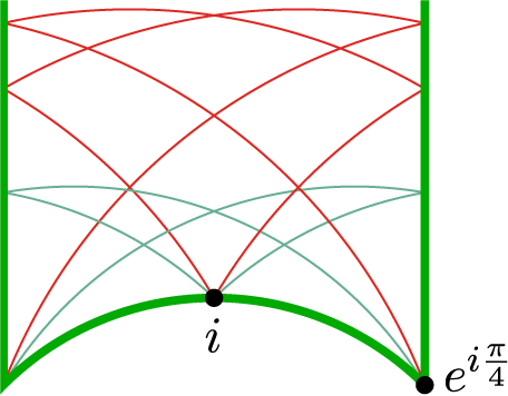


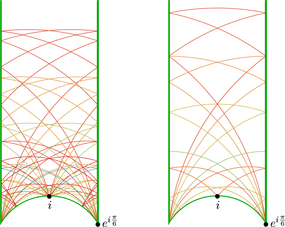


 Open access