


1. Introduction
Recent years have seen an increasing interest towards a particular class of unconventional marine propellers, the rim driven thrusters (RDTs), as reported by Yan et al. (Reference Yan, Liang, Ouyang, Liu, Liu and Lan2017), Nuchturee, Li & Xia (Reference Nuchturee, Li and Xia2020) and Wang et al. (Reference Wang, Li, Zhang, Ma, Huang, Wang and Jiang2025). They share similarities with ducted propellers, since their rotor operates within a stationary nozzle. Compared with conventional propellers, the presence of a nozzle determines different advantages, depending on its geometry. For instance, accelerating nozzles contribute to the thrust produced by the overall system, improving its propulsive efficiency. This means they are able to produce the same thrust, but requiring a smaller torque to move the rotor of the propeller. In contrast, decelerating nozzles produce a negative thrust, but they have the advantage of mitigating the negative peak of pressure within the propeller and, in turn, the onset of unwanted cavitation phenomena, with benefits in terms of vibrations, noise and structural damage. However, typical ducted propellers are affected by the issue of the leakage flow between the tip of the rotor blades and the inner surface of the nozzle. This is a location of friction losses, pressure minima (potential cavitation) and large turbulence. In addition, they still need a rotating hub to move their rotor blades. This causes the onset of a large axial vortex populating the wake of the propeller, which is also a location of potential cavitation phenomena and large turbulent stresses. Its interaction with downstream devices, such as rudders, is especially problematic, since it is an additional, important source of erosion, vibrations and noise (Zhang et al. Reference Zhang, Li, Ma, Ning, Sun and Hu2022; Posa et al. Reference Posa, Broglia, Balaras and Felli2023; Pendar & Oshkai Reference Pendar and Oshkai2025). The RDTs differ from typical ducted propellers, since their blades are not mounted on a rotating hub, but instead on a rim rotating within a slot in their nozzle. This solution eliminates the issue of the leakage flow produced between the tip of the blades and the nozzle, since there is no gap between them, replaced by the gap between the rim and the statoric part of the propeller. In addition, RDTs do not need a rotating hub, which causes the onset of the axial vortex characterising the wake of conventional propellers. It is worth mentioning that the concept of RDTs is actually not very new, dating back to the 1950s (Saunders Reference Saunders1957). However, only the recent development of compact, brushless electric motors, which can be mounted directly within the nozzle of the propellers, has allowed the practical implementation of this idea.
The study of marine propellers is not a trivial task, through both experiments and numerical simulations, due to the presence of parts in relative motion and the complexity of their flow physics. However, the last two decades have seen several studies dealing with more conventional marine propellers (see only a few examples by Felli et al. Reference Felli, Di Felice, Guj and Camussi2006, Reference Felli, Guj and Camussi2008, Reference Felli, Camussi and Di Felice2011; Baek et al. Reference Baek, Yoon, Jung, Kim and Paik2015; Balaras, Schroeder & Posa Reference Balaras, Schroeder and Posa2015; Kumar & Mahesh Reference Kumar and Mahesh2017; Felli & Falchi Reference Felli and Falchi2018; Wang et al. Reference Wang, Guo, Su and Wu2018, Reference Wang, Wu, Gong and Yang2021, Reference Wang, Li, Guo, Wang and Sun2022, Reference Wang, Liu, Guo, Li and Liao2023; Cianferra, Petronio & Armenio Reference Cianferra, Petronio and Armenio2019; Ahmed, Croaker & Doolan Reference Ahmed, Croaker and Doolan2020; Sun et al. Reference Sun, Wang, Guo, Zhang, Sun and Liu2020; Petris, Cianferra & Armenio Reference Petris, Cianferra and Armenio2022; Sun & Wang Reference Sun and Wang2022; Posa & Broglia Reference Posa and Broglia2025; Wu et al. Reference Wu, Wang, Hu and Luo2025). Through both experiments and numerical simulations, they clarified that the tip vortices experience short-wave and long-wave instability phenomena, leading to mutual inductance and coupling events, and eventually to break-up into smaller scales. This dynamics was found in agreement with the earlier theoretical work on the instability process of helical vortices by Widnall (Reference Widnall1972). The existing literature also agrees on the behaviour of the hub vortex. This is the largest, most intense flow structure populating the wake. It is also more stable than the tip vortices, which means it is the one having the most long-standing impact on the wake signature of marine propellers, experiencing fluctuations of its trajectory and eventual break-up at distances further downstream from the propeller, if compared with the tip vortices. Therefore, a propulsion system able to avoid this large vortex is potentially able to achieve important benefits in terms of radiated sound and interaction with downstream rudders, which is a source of complex fluid dynamics. This interaction was the subject of a number of recent studies (Felli & Falchi Reference Felli and Falchi2011; Wang et al. Reference Wang, Guo, Xu and Su2019; Posa, Broglia & Balaras Reference Posa, Broglia and Balaras2020; Posa & Broglia Reference Posa and Broglia2021; Posa Reference Posa2023b ; Zhang et al. Reference Zhang, Li, Sun, Zhang, Chen and Hu2023). Ducted propellers are able to improve performance in terms of efficiency of propulsion (Bontempo & Manna Reference Bontempo and Manna2018) or cavitation inception (Bontempo, Cardone & Manna Reference Bontempo, Cardone and Manna2016), depending on the accelerating or decelerating actions of the nozzle, as discussed in the works by Gaggero et al. (Reference Gaggero, Villa, Tani, Viviani and Bertetta2017) and Villa et al. (Reference Villa, Gaggero, Tani and Viviani2020). However, they do not eliminate the issues arising from the onset of a large axial vortex (Gong et al. Reference Gong, Guo, Zhao, Wu and Song2018, Reference Gong, Ding and Wang2021; Stark & Shi Reference Stark and Shi2021; Posa & Broglia Reference Posa and Broglia2025).
In contrast with the extensive literature on conventional propellers, the work done on RDTs is still quite limited, due to the novelty of their practical implementation as marine propulsion devices. Meanwhile, as suggested already, important changes are expected to affect their flow physics, if compared with more conventional propellers, making them a subject of great theoretical and practical interest. Most of the current studies on RDTs are focused on their hydrodynamic performance, with little discussion on their flow physics (Cao et al. Reference Cao, Hong, Tang, Hu and Lu2012; Song, Wang & Tian Reference Song, Wang and Tian2015; Liu & Vanierschot Reference Liu and Vanierschot2021). In these cases, the Reynolds-averaged Navier–Stokes (RANS) equations are resolved. This technique is considered accurate enough when the global parameters of performance are the major subject of interest. For instance, this strategy was adopted in the framework of algorithms of optimisation of the performance of these propulsion devices (Gaggero Reference Gaggero2020; Liu et al. Reference Liu, Jiang, Liu, Yu and Bian2022b ; Zhai et al. Reference Zhai, Jin, Chen, Liu and Song2022; Liu, Dai & Liang Reference Liu, Vanierschot and Buysschaert2023c ; Nie et al. Reference Nie, Ouyang, Zhang, Li and Zheng2023). RANS was also used by Cai et al. (Reference Cai, Tian, Qiu, Xu, Mao, He and Chai2022) for the development of a body force technique by using virtual disks to represent the action of RDTs on the flow without resolving explicitly their geometry, with the purpose of saving computational resources. In addition, a number of works employed RANS computations to study the influence of the gap between the rim and the statoric part of the propeller on its overall performance (Li et al. Reference Li, Yao, Wang and Weng2023b ; Lin et al. Reference Lin, Yao, Wang, Su and Yang2023; Liu et al. Reference Liu, Dai and Liang2023a ; Cai et al. Reference Cai, Xu, Tian, Qiu, Chai, Qi and He2024). Although the influence on performance was revealed, the impact on the flow physics outside the gap region was found practically negligible. A transition model for RANS was used by Liu et al. (Reference Liu, Vanierschot and Buysschaert2022a ) to explore the effect on performance of changing the geometry of the nozzle at Reynolds numbers typical of underwater remotely operated vehicles (ROVs) or autonomous underwater vehicles (AUVs). They verified indeed an improved agreement with the experiments by including the transition model in the RANS computations. By using a similar approach, Liu et al. (Reference Liu, Vanierschot and Buysschaert2023b ) analysed the influence of scale effects on the performance of an RDT, by using a transition model to simulate the propeller at model scale and compare with the full scale case. They found that scale effects influence the performance of the nozzle and the rim more than that of the rotor blades. They produce a reduction for the torque coefficient from model scale to full scale, while the thrust coefficient is little modified, which means an improved efficiency of propulsion. Some RANS studies (Jiang et al. Reference Jiang, Ouyang, Sheng, Lan and Bucknall2022; Chen et al. Reference Chen, Chen, Zhou, Zhang, Chen and Zheng2023) even considered contra-rotating RDTs, consisting of two rotors with opposite angular speeds. The downstream one has the purpose of recovering the azimuthal momentum gained by the flow through the front rotor. This strategy increases the overall efficiency of propulsion and reduces the lateral loads experienced by the system. In other cases, an improved efficiency is pursued by statoric blades, mimicking the approach adopted in pumpjet propellers, as in the studies by Dubas, Bressloff & Sharkh (Reference Dubas, Bressloff and Sharkh2015) and Yang, Li & Zhang (Reference Yang, Li and Zhang2024). In the work by Liu et al. (Reference Liu, Ouyang, Yan and Vanierschot2024a ), the performance of an RDT was also tested when mounted at the tail of an underwater vehicle, the theoretical submarine geometry of the DARPA suboff (Liu & Huang Reference Liu and Huang1998). Comparisons with the performance of the isolated propeller were also reported.
However, as well known from the literature, RANS is usually not accurate enough if the focus is on the fluid dynamics, the wake instability and the statistics of turbulence (Muscari, Di Mascio & Verzicco Reference Muscari, Di Mascio and Verzicco2013; Cai, Li & Liu Reference Cai, Li and Liu2019; Sezen, Atlar & Fitzsimmons Reference Sezen, Atlar and Fitzsimmons2021). Therefore, in the last few years, a few eddy-resolving simulations were reported in the field of RDTs to gain a better understanding of their flow physics affecting their wake signature. For instance, Gaggero (Reference Gaggero2023) used improved delayed detached eddy simulation (IDDES) to analyse the wake flow of a four-bladed and two six-bladed RDTs, including also a conventional ducted propeller producing the same thrust. A finite volume approach was adopted, using computational grids consisting of 44 million and 66 million cells for the unconventional and conventional propellers, respectively. The higher resolution in the latter case was required by the need of resolving the leakage flow at the tip of its blades. The simulations demonstrated a significant reduction of the intensity of the pressure fluctuations within the wake system of the RDTs, if compared with the conventional ducted propeller. This was found the result of the weaker and more stable vortices populating the downstream flow in the former case, both at the outer boundary of the wake, dominated by the shear layer shed from the nozzle, and within the wake core. This study presents also a comparison between IDDES and RANS results, confirming the improved accuracy of the former, compared with the latter, which are negatively affected by a faster dissipation of the wake structures.
DDES was also adopted by Li et al. (Reference Li, Sun, Yao, Wang, Wang and Weng2023a ) to study the influence of the criterion of domain decomposition on the solution of the flow through an RDT equipped with both front and rear stator blades. Computational meshes consisting of a number of finite volumes up to 27 million were used. Although some wake features were reported, this work was mainly focused on the global performance of the propeller and the gap flow between the rim and the nozzle. An interesting study was also conducted by Liu et al. (Reference Liu, Yan, Ouyang and Vanierschot2024b ) on the comparison between the wake systems of a conventional ducted propeller and an RDT in bollard condition. This is a working condition far away from design: the propellers operate with an advance velocity equal to 0, shedding intense flow structures in their wake. In this study, DDES computations on grids up to 24.5 million finite volumes were carried out. Again, the results of the simulations highlight the advantage of the missing gap flow between the tip of the propeller blades and the nozzle in the RDT, decreasing the levels of pressure fluctuations at the outermost radii and the intensity of the flow structures populating the outer boundary of the wake. It is worth mentioning that in this study, the two propellers only differ for the absence of the tip gap in the RDT, which still has a rotating hub, producing an axial vortex similar to that shed by the conventional propeller.
Yang et al. (Reference Yang, Yao, Sun, Wang, Guo and Lin2025) computed a two-way coupled fluid structure interaction problem on an RDT. They used IDDES to resolve the fluid dynamics on a computational grid consisting of 16 million finite volumes and a finite element method to resolve the deformation of the propeller blades, by considering the stiffness properties of different materials (steel alloy, copper alloy, fibreglass and resin fibre). In addition to the deformation of the propeller blades, they compared the performance and wake flow, including also the case of rigid blades as a benchmark for reference. They found that decreasing values of the Young modulus, producing larger deformations of the propeller blades, especially in the axial direction, result in reduced hydrodynamic performance and higher turbulent fluctuations. In the study by Zhang et al. (Reference Zhang, Liu, Ouyang, Zheng and Vanierschot2025), the energy losses affecting an RDT were analysed by coupling the entropy production theory and results of numerical simulations by RANS and DES, carried out on computational grids of up to 35 million finite volumes. This study reported that the major near wall entropy production occurs on the rotating parts of the propeller and is in particular associated with the rim. As expected, the most important source of losses in the wake flow is due to the instability of the wake structures, affecting especially those populating the shear layer from the trailing edge of the nozzle.
The DES studies reported previously demonstrated their higher accuracy, if compared with RANS. They were able to provide more details on the flow physics of this class of propellers, in agreement with the earlier literature on more conventional propellers. This improved accuracy comes from finer computational grids, consisting of $\mathcal{O}(10^7)$
cells, and the inherent features of DES, resolving the filtered Navier–Stokes equations away from the surface of the bodies immersed within the flow and restricting the RANS strategy to the only near-wall region. In this study, a significant step forward in the same direction is reported, by presenting results of LES computations conducted on grids of
$\mathcal{O}(10^7)$
cells, and the inherent features of DES, resolving the filtered Navier–Stokes equations away from the surface of the bodies immersed within the flow and restricting the RANS strategy to the only near-wall region. In this study, a significant step forward in the same direction is reported, by presenting results of LES computations conducted on grids of $\mathcal{O}(10^9)$
points. They deal with a conventional ducted propeller and an RDT, sharing the same geometry of their nozzle and designed to produce the same overall thrust. A detailed comparison of the flow across the propellers and in their wake is discussed. It is worth mentioning that a similar comparison was conducted by Liu et al. (Reference Liu, Yan, Ouyang and Vanierschot2024b
) using DDES on a coarser mesh, but with important differences from the present work. Their strategy was to compare two propellers having the same geometry and differing only for the radial gap between the tip of their blades and the nozzle in the conventional propeller. Their purpose was to isolate the effect of the absence of the leakage flow in that region, which is beneficial to RDTs. In contrast, in the present study, the differences between the geometries of the two propellers are more substantial, exploiting all advantages of RDTs. They are not limited to the absence of the leakage flow at the tip of the blades. They include also the lack of a rotating hub, which is not needed anymore in RDTs, and a more uniform distribution of the load across the span of the blades. This keeps higher values at the outermost radii than in conventional propellers, with advantages in terms of performance. Therefore, in this study, the predictive capabilities of LES as well as the fine resolution of the computational grid are exploited to resolve a wide range of turbulent scales and analyse the multiple phenomena contributing to the substantial modification of the flow physics of RDTs, compared with that of conventional ducted propellers. These differences affect both the flow across the blades and the wake system. We will show that the more uniform distribution of the load across the blades of the RDT produces a mitigation of the cross-flow instabilities of the boundary layer, which are promoted by centrifugal effects (Jing & Ducoin Reference Jing and Ducoin2020; Boudenne & Ducoin Reference Boudenne and Ducoin2024), but also reinforced by spanwise variations of the load. These changes will be shown to result in smaller streamwise vortices and lower turbulent stresses both across the propeller blades and in their trailing wake. Meanwhile, the lack of both leakage vortices and a large hub vortex contributes to a substantially lower intensity of the pressure minima and turbulent stresses on the inner surface of the nozzle and within the wake core, with potential benefits to the acoustic signature of RDTs. In particular, the large axial vortex shed by conventional propellers experiences high levels of shear with the surrounding flow, accelerated by the propeller blades. This shear is an important source of turbulence production, as reported in the following discussion. Therefore, the absence of the hub vortex downstream of RDTs results in a dramatic reduction of the turbulent stresses at the wake core as well as a slower development of instability phenomena, especially at the innermost radial coordinates of the wake system.
$\mathcal{O}(10^9)$
points. They deal with a conventional ducted propeller and an RDT, sharing the same geometry of their nozzle and designed to produce the same overall thrust. A detailed comparison of the flow across the propellers and in their wake is discussed. It is worth mentioning that a similar comparison was conducted by Liu et al. (Reference Liu, Yan, Ouyang and Vanierschot2024b
) using DDES on a coarser mesh, but with important differences from the present work. Their strategy was to compare two propellers having the same geometry and differing only for the radial gap between the tip of their blades and the nozzle in the conventional propeller. Their purpose was to isolate the effect of the absence of the leakage flow in that region, which is beneficial to RDTs. In contrast, in the present study, the differences between the geometries of the two propellers are more substantial, exploiting all advantages of RDTs. They are not limited to the absence of the leakage flow at the tip of the blades. They include also the lack of a rotating hub, which is not needed anymore in RDTs, and a more uniform distribution of the load across the span of the blades. This keeps higher values at the outermost radii than in conventional propellers, with advantages in terms of performance. Therefore, in this study, the predictive capabilities of LES as well as the fine resolution of the computational grid are exploited to resolve a wide range of turbulent scales and analyse the multiple phenomena contributing to the substantial modification of the flow physics of RDTs, compared with that of conventional ducted propellers. These differences affect both the flow across the blades and the wake system. We will show that the more uniform distribution of the load across the blades of the RDT produces a mitigation of the cross-flow instabilities of the boundary layer, which are promoted by centrifugal effects (Jing & Ducoin Reference Jing and Ducoin2020; Boudenne & Ducoin Reference Boudenne and Ducoin2024), but also reinforced by spanwise variations of the load. These changes will be shown to result in smaller streamwise vortices and lower turbulent stresses both across the propeller blades and in their trailing wake. Meanwhile, the lack of both leakage vortices and a large hub vortex contributes to a substantially lower intensity of the pressure minima and turbulent stresses on the inner surface of the nozzle and within the wake core, with potential benefits to the acoustic signature of RDTs. In particular, the large axial vortex shed by conventional propellers experiences high levels of shear with the surrounding flow, accelerated by the propeller blades. This shear is an important source of turbulence production, as reported in the following discussion. Therefore, the absence of the hub vortex downstream of RDTs results in a dramatic reduction of the turbulent stresses at the wake core as well as a slower development of instability phenomena, especially at the innermost radial coordinates of the wake system.
The present manuscript is structured as follows: the methodology in § 2; the flow problem in § 3; the computational set-up in § 4; the analysis of the results in § 5, including the discussion of the flow across the propellers and within their wake; and the conclusions in § 6.
2. Methodology
The problem was resolved through the filtered Navier–Stokes equations for incompressible flows in non-dimensional form:
 \begin{eqnarray} {\partial \widetilde {u}_i \over \partial x_i} = 0, \;\;\; i=1,2,3, \end{eqnarray}
 \begin{eqnarray} {\partial \widetilde {u}_i \over \partial t} + {\partial \widetilde {u}_i \widetilde {u}_{\!j} \over \partial x_{\!j} } = - {\partial \tilde {p} \over \partial x_i} - {\partial \tau _{\textit{ij}} \over \partial x_{\!j}} + {1 \over \mathit{Re}} {\partial ^2 \widetilde {u}_i \over \partial x_{\!j}^2} + f_i, \;\;\;i,j=1,2,3, \end{eqnarray}
where (2.1) and (2.2) represent the conservation of mass and momentum, respectively. In those equations, $x_i$
is the coordinate in the direction
$x_i$
is the coordinate in the direction $i$
in space,
$i$
in space, $t$
is time,
$t$
is time, $\widetilde {u}_i$
the filtered velocity component in the direction
$\widetilde {u}_i$
the filtered velocity component in the direction $i$
,
$i$
, $\tilde {p}$
the filtered pressure,
$\tilde {p}$
the filtered pressure, $\tau _{\textit{ij}}$
the
$\tau _{\textit{ij}}$
the $ij$
element of the subgrid scale (SGS) stress tensor,
$ij$
element of the subgrid scale (SGS) stress tensor, $\mathit{Re}$
the Reynolds number and
$\mathit{Re}$
the Reynolds number and $f_i$
the component in the direction
$f_i$
the component in the direction $i$
of a forcing term. The Reynolds number results from scaling the equations by the density of the fluid,
$i$
of a forcing term. The Reynolds number results from scaling the equations by the density of the fluid, $\rho$
, a reference length scale,
$\rho$
, a reference length scale, $\mathcal{L}$
, and a reference velocity scale,
$\mathcal{L}$
, and a reference velocity scale, $\mathcal{V}$
, and is defined as
$\mathcal{V}$
, and is defined as $\mathit{Re}=\mathcal{LV}/\nu$
, where
$\mathit{Re}=\mathcal{LV}/\nu$
, where $\nu$
is the kinematic viscosity of the fluid. The equations are filtered, which means that only the scales larger than the size of the filter,
$\nu$
is the kinematic viscosity of the fluid. The equations are filtered, which means that only the scales larger than the size of the filter, $\varDelta$
, are resolved, while the smaller ones are modelled. The size of the filter is implicitly defined by the local resolution of the computational grid adopted to resolve the flow.
$\varDelta$
, are resolved, while the smaller ones are modelled. The size of the filter is implicitly defined by the local resolution of the computational grid adopted to resolve the flow.
The SGS tensor, $\tau _{\textit{ij}}=\widetilde {u_i u_{\!j}}-\widetilde {u}_i \widetilde {u}_{\!j}$
, comes from filtering the nonlinear terms of the momentum equation and represents the action of the scales smaller than the filter on the larger ones. It is required to be modelled to close the turbulence problem. In this work, this closure is based on the Boussinesq hypothesis. This assumes that the deformation tensor of the resolved velocity field,
$\tau _{\textit{ij}}=\widetilde {u_i u_{\!j}}-\widetilde {u}_i \widetilde {u}_{\!j}$
, comes from filtering the nonlinear terms of the momentum equation and represents the action of the scales smaller than the filter on the larger ones. It is required to be modelled to close the turbulence problem. In this work, this closure is based on the Boussinesq hypothesis. This assumes that the deformation tensor of the resolved velocity field, $\widetilde {S}_{\textit{ij}}$
, and the deviatoric part of the SGS tensor,
$\widetilde {S}_{\textit{ij}}$
, and the deviatoric part of the SGS tensor, $\tau _{\textit{ij}}^d$
, are aligned:
$\tau _{\textit{ij}}^d$
, are aligned:
 \begin{equation} \tau _{\textit{ij}}^d = \tau _{\textit{ij}} - {1 \over 3} \delta _{\textit{ij}} \tau _{kk} = -2 \nu _t \widetilde {S}_{\textit{ij}}, \;\;\;i,j=1,2,3, \end{equation}
where $\delta _{\textit{ij}}$
is the Kronecker delta,
$\delta _{\textit{ij}}$
is the Kronecker delta, $\tau _{kk}$
the trace of the SGS tensor and
$\tau _{kk}$
the trace of the SGS tensor and $\nu _t$
the eddy-viscosity. This hypothesis allows reducing the number of unknowns of the problem from the six independent components of the symmetric SGS tensor to the only eddy-viscosity. This quantity was computed by using the wall-adaptive local eddy-viscosity (WALE) model by Nicoud & Ducros (Reference Nicoud and Ducros1999):
$\nu _t$
the eddy-viscosity. This hypothesis allows reducing the number of unknowns of the problem from the six independent components of the symmetric SGS tensor to the only eddy-viscosity. This quantity was computed by using the wall-adaptive local eddy-viscosity (WALE) model by Nicoud & Ducros (Reference Nicoud and Ducros1999):
 \begin{equation} \nu _t= (C_W \Delta )^2 {\left ( \kern2pt \widetilde {\kern-2pt \mathcal{S}}_{\textit{ij}}^{\kern1pt d} \kern2pt \widetilde {\kern-2pt \mathcal{S}}_{\textit{ij}}^{\kern1pt d} \right )^{3/2} \over \left ( \widetilde {S}_{\textit{ij}} \widetilde {S}_{\textit{ij}} \right )^{5/2} + {\left ( \kern2pt \widetilde {\kern-2pt \mathcal{S}}_{\textit{ij}}^{\kern1pt d} \kern2pt \widetilde {\kern-2pt \mathcal{S}}_{\textit{ij}}^{\kern1pt d} \right )^{5/4}}}, \;\;\;i,j=1,2,3, \end{equation}
where $C_W=0.5$
is a constant,
$C_W=0.5$
is a constant, $\kern2pt \widetilde {\kern-2pt \mathcal{S}}_{\textit{ij}}^{\kern1pt d}$
is the deviatoric part of the square of the gradient of the filtered velocity field, while
$\kern2pt \widetilde {\kern-2pt \mathcal{S}}_{\textit{ij}}^{\kern1pt d}$
is the deviatoric part of the square of the gradient of the filtered velocity field, while $\varDelta$
(the size of the filter) was computed as the cube root of the local size of the cells of the computational grid where the flow problem was resolved. Here,
$\varDelta$
(the size of the filter) was computed as the cube root of the local size of the cells of the computational grid where the flow problem was resolved. Here, $\kern2pt \widetilde {\kern-2pt \mathcal{S}}_{\textit{ij}}^{\kern1pt d}$
takes into account both the deformation and rotation tensors of the filtered velocity field, which enables the model to switch off in areas of laminar gradients. Furthermore, the model was designed to reproduce the correct evolution of the eddy-viscosity in the vicinity of solid walls, scaling as the cube of the distance from the wall. Therefore, the WALE model does not need near-wall corrections to switch off, which may be complicated to implement on complex geometries. Furthermore, it is computationally inexpensive, if compared, for instance, with the dynamic Smagorinsky model (Germano et al. Reference Germano, Piomelli, Moin and Cabot1991; Meneveau & Lund Reference Meneveau and Lund1997). This is an important, convenient feature, given the large size of the present simulations. Its computational cost is indeed equivalent to only a few percent of the overall one. Its choice was based on our extensive experience, demonstrating the accuracy of the WALE model in a number of earlier studies (Posa & Balaras Reference Posa and Balaras2016, Reference Posa and Balaras2018, Reference Posa and Balaras2020; Posa, Broglia & Balaras Reference Posa, Broglia and Balaras2022), including also detailed comparisons with experiments.
$\kern2pt \widetilde {\kern-2pt \mathcal{S}}_{\textit{ij}}^{\kern1pt d}$
takes into account both the deformation and rotation tensors of the filtered velocity field, which enables the model to switch off in areas of laminar gradients. Furthermore, the model was designed to reproduce the correct evolution of the eddy-viscosity in the vicinity of solid walls, scaling as the cube of the distance from the wall. Therefore, the WALE model does not need near-wall corrections to switch off, which may be complicated to implement on complex geometries. Furthermore, it is computationally inexpensive, if compared, for instance, with the dynamic Smagorinsky model (Germano et al. Reference Germano, Piomelli, Moin and Cabot1991; Meneveau & Lund Reference Meneveau and Lund1997). This is an important, convenient feature, given the large size of the present simulations. Its computational cost is indeed equivalent to only a few percent of the overall one. Its choice was based on our extensive experience, demonstrating the accuracy of the WALE model in a number of earlier studies (Posa & Balaras Reference Posa and Balaras2016, Reference Posa and Balaras2018, Reference Posa and Balaras2020; Posa, Broglia & Balaras Reference Posa, Broglia and Balaras2022), including also detailed comparisons with experiments.
The forcing term, $f_i$
, in the momentum equation was used in this study to enforce the no-slip boundary condition on solid walls, by using an immersed boundary (IB) technique. Therefore, the flow problem was resolved on a regular, stationary Eulerian grid, not conforming to the geometry of the bodies immersed within the flow. Their surface was instead represented by unstructured, Lagrangian grids, immersed within the Eulerian grid and free to move across its cells. The points of the Eulerian grid were tagged as solid, fluid and interface, based on their position relative to the Lagrangian grids representing the immersed boundaries. The solid points were defined as those placed within the immersed boundaries, while the interface points were those placed outside, but having a solid neighbour along any coordinate direction. All remaining points were defined as fluid points. At the fluid points, no boundary conditions were required and the values of the flow variables there were computed from the solution of the Navier–Stokes equations. In contrast, at the solid points, a velocity condition was enforced, equal to the local velocity of the body where each particular solid point was placed. At the interface points, the velocity condition came from a linear reconstruction of the solution in the local direction normal to the Lagrangian grid representing the immersed boundary. This reconstruction used as boundary conditions the no-slip requirement on the surface of the body and the solution of the flow at the fluid points surrounding the particular interface point. Then, the forcing term (equal to 0 at the fluid points) at the solid and interface points was computed as
$f_i$
, in the momentum equation was used in this study to enforce the no-slip boundary condition on solid walls, by using an immersed boundary (IB) technique. Therefore, the flow problem was resolved on a regular, stationary Eulerian grid, not conforming to the geometry of the bodies immersed within the flow. Their surface was instead represented by unstructured, Lagrangian grids, immersed within the Eulerian grid and free to move across its cells. The points of the Eulerian grid were tagged as solid, fluid and interface, based on their position relative to the Lagrangian grids representing the immersed boundaries. The solid points were defined as those placed within the immersed boundaries, while the interface points were those placed outside, but having a solid neighbour along any coordinate direction. All remaining points were defined as fluid points. At the fluid points, no boundary conditions were required and the values of the flow variables there were computed from the solution of the Navier–Stokes equations. In contrast, at the solid points, a velocity condition was enforced, equal to the local velocity of the body where each particular solid point was placed. At the interface points, the velocity condition came from a linear reconstruction of the solution in the local direction normal to the Lagrangian grid representing the immersed boundary. This reconstruction used as boundary conditions the no-slip requirement on the surface of the body and the solution of the flow at the fluid points surrounding the particular interface point. Then, the forcing term (equal to 0 at the fluid points) at the solid and interface points was computed as
 \begin{equation} f_i = {\mathcal{U}_i - \widetilde {u}_i \over \Delta t} - \widetilde {\mathcal{R}}_i, \;\;\; i=1,2,3, \end{equation}
where $\mathcal{U}_i$
is the velocity boundary condition in the direction
$\mathcal{U}_i$
is the velocity boundary condition in the direction $i$
, defined as discussed previously,
$i$
, defined as discussed previously, $\widetilde {u}_i$
the local solution of the flow at the particular solid or interface point,
$\widetilde {u}_i$
the local solution of the flow at the particular solid or interface point, $\Delta t$
the step of advancement in time of the numerical solution and
$\Delta t$
the step of advancement in time of the numerical solution and $\widetilde {\mathcal{R}}_i$
the sum of the convective, viscous, SGS and pressure gradient terms of the momentum equation at that point, all computed explicitly from the filtered velocity and pressure fields. It is also important to point out that in all the following discussion, only resolved velocity and pressure fields will be considered. Therefore, for convenience, the tilde notation
$\widetilde {\mathcal{R}}_i$
the sum of the convective, viscous, SGS and pressure gradient terms of the momentum equation at that point, all computed explicitly from the filtered velocity and pressure fields. It is also important to point out that in all the following discussion, only resolved velocity and pressure fields will be considered. Therefore, for convenience, the tilde notation $\widetilde {\mathcal{P}}$
used to indicate any filtered physical quantity,
$\widetilde {\mathcal{P}}$
used to indicate any filtered physical quantity, $\mathcal{P}$
, will be omitted hereafter.
$\mathcal{P}$
, will be omitted hereafter.
Equations (2.1) and (2.2) were numerically resolved on a staggered cylindrical grid. Their discretisation in space used second-order central differences. As demonstrated by Fukagata & Kasagi (Reference Fukagata and Kasagi2002), this strategy achieves the exact conservation of mass, momentum and energy by the discretised version of the equations. The advancement in time used a fractional-step method (Van Kan Reference Van Kan1986). The discretisation in time was based on the explicit, three-step Runge–Kutta scheme. However, to relax the stability restrictions to the time step, due to the local resolution in space of the cylindrical grid, all convective, viscous and SGS terms of azimuthal derivatives in the vicinity of the axis of the cylindrical grid were advanced in time using the implicit Crank–Nicolson scheme. The same strategy was adopted for the terms of radial derivatives in the vicinity of the inner surface of the nozzle. As discussed in more detail in § 4, there the radial resolution of the cylindrical grid was significantly refined, with the purpose of resolving the leakage flow between the tip of the propeller blades and the nozzle. The discretisation of the continuity equation resulted in a hepta-diagonal Poisson problem. This was resolved by decomposing the hepta-diagonal system of equations in a series of penta-diagonal problems, by means of trigonometric transformations along the periodic azimuthal direction. Then, each penta-diagonal problem was inverted by means of an efficient direct solver (Rossi & Toivanen Reference Rossi and Toivanen1999). More details on the particular implementation of the IB technique and the overall Navier–Stokes solver considered in this study are reported in the works by Balaras (Reference Balaras2004) and Yang & Balaras (Reference Yang and Balaras2006), where it was demonstrated to be second-order accurate in both space and time. It was successfully adopted for the solution of the flow dealing with marine propellers, as demonstrated in a number of works (Posa Reference Posa2022, Reference Posa2023a ; Posa et al. Reference Posa, Broglia, Shi and Felli2024a , Reference Posa, Capone, Alves Pereira, Di Felice and Brogliab ), including also validations with physical experiments for both performance and flow fields in the wake.
Geometries of (a,c,e) the conventional ducted propeller ( $\mathrm{DP}$
) and (b,d, f) the rim driven thruster (
$\mathrm{DP}$
) and (b,d, f) the rim driven thruster ( $\mathrm{RDT}$
): (a,b) isometric views from upstream, (c,d) isometric views from downstream, (e, f) frontal views of a blade. Stators and rotors represented in orange and light blue colours, respectively.
$\mathrm{RDT}$
): (a,b) isometric views from upstream, (c,d) isometric views from downstream, (e, f) frontal views of a blade. Stators and rotors represented in orange and light blue colours, respectively. $\varOmega = 2 \pi n$
representing the angular speed of the rotors.
$\varOmega = 2 \pi n$
representing the angular speed of the rotors.

3. Flow problem
Two four-bladed marine propellers were simulated. They are illustrated in figure 1. The propeller shown in figure 1(a,c,e) is a ducted propeller, indicated hereafter also as $\mathrm{DP}$
, with its blades installed on a rotating shaft. They are characterised by a strong three-dimensional development, achieving their peak load at approximately
$\mathrm{DP}$
, with its blades installed on a rotating shaft. They are characterised by a strong three-dimensional development, achieving their peak load at approximately $70\,\%$
of their radial extent, which is typical of conventional marine propellers. This strategy is adopted to decrease the intensity of the root and hub vortices at the innermost radial coordinates and the one of the tip vortices (or leakage flows in the case of ducted propellers) at the outermost radial coordinates. Note also that the complex geometry of the hub is the actual one of this particular propeller and is required for installation purposes of the controllable pitch blades. As shown in the following discussion of the fluid dynamics, the sharp edges characterising the geometry of the hub are sources of intense shear layers populating the near wake of this propeller. The geometry in figure 1(b,d, f) is that of a rim driven thruster, indicated hereafter as
$70\,\%$
of their radial extent, which is typical of conventional marine propellers. This strategy is adopted to decrease the intensity of the root and hub vortices at the innermost radial coordinates and the one of the tip vortices (or leakage flows in the case of ducted propellers) at the outermost radial coordinates. Note also that the complex geometry of the hub is the actual one of this particular propeller and is required for installation purposes of the controllable pitch blades. As shown in the following discussion of the fluid dynamics, the sharp edges characterising the geometry of the hub are sources of intense shear layers populating the near wake of this propeller. The geometry in figure 1(b,d, f) is that of a rim driven thruster, indicated hereafter as $\mathrm{RDT}$
, whose blades are installed on a rim rotating within the nozzle. No rotating hub is required in this case to move the blades of the propeller. As shown by the geometry of the blades of this propeller, the distribution of the load across their span is more uniform, if compared with
$\mathrm{RDT}$
, whose blades are installed on a rim rotating within the nozzle. No rotating hub is required in this case to move the blades of the propeller. As shown by the geometry of the blades of this propeller, the distribution of the load across their span is more uniform, if compared with $\mathrm{DP}$
, thanks to the lack of both hub and leakage between the tip of the blades and the nozzle. The geometry of the nozzle is shared between the two propellers.
$\mathrm{DP}$
, thanks to the lack of both hub and leakage between the tip of the blades and the nozzle. The geometry of the nozzle is shared between the two propellers.
Both propellers were designed to deliver the same overall thrust with the same criteria of maximisation of efficiency and minimisation of cavitation risk (however, about this point, it is important to mention that the numerical model considered in this study does not include cavitation). These requirements led to the adoption of a decelerating nozzle. Compared with accelerating nozzles, commonly employed to increase thrust, especially under bollard-pull conditions (i.e. at very low advance speeds), decelerating nozzles raise the static pressure within the duct, with the purpose of delaying the onset of cavitation phenomena on their blades. This benefit, however, comes at the expense of an additional drag produced by the nozzle itself, with a negative impact on propulsive efficiency, affecting also the vortical structures shed in the wake. Accelerating nozzles increase the velocity of the flow entering the rotor. This acceleration produces smaller angles of incidence and a reduced load on the propeller blades, partially compensated by the additional thrust generated by the nozzle itself. As a result, accelerating nozzles typically yield higher propulsive efficiency. Decelerating nozzles produce instead stronger adverse pressure gradients, especially on the outer surface of the duct, promoting more intense vortex shedding compared with accelerating nozzles. By reducing the velocity of the incoming flow, they also shift the effective advance coefficient experienced by the rotor towards lower values, increasing the blade load. Consequently, more intense flow structures are shed in the trailing wake of the propeller blades. In addition, the helical vortices shed by the rotor and the trailing wakes of the blades exhibit a smaller pitch, which intensifies mutual inductance phenomena and accelerates wake instability.
Main geometrical parameters of the propellers.

Sections of the geometries of (a) the conventional ducted propeller and (b) the rim driven thruster across their blades.

The need to minimise cavitation risk and the different flow features arising from the presence (in the case of $\mathrm{DP}$
) or absence (in the case of
$\mathrm{DP}$
) or absence (in the case of $\mathrm{RDT}$
) of a tip gap, strongly influence also the blade design. The blades of a conventional ducted propeller, as the
$\mathrm{RDT}$
) of a tip gap, strongly influence also the blade design. The blades of a conventional ducted propeller, as the $\mathrm{DP}$
geometry considered in this study, exhibit a pronounced three-dimensional development. They were designed following the approach described by Gaggero et al. (Reference Gaggero, Rizzo, Tani and Viviani2012, Reference Gaggero, Rizzo, Tani and Viviani2013, Reference Gaggero, Tani, Viviani and Conti2014), with their peak load located at approximately
$\mathrm{DP}$
geometry considered in this study, exhibit a pronounced three-dimensional development. They were designed following the approach described by Gaggero et al. (Reference Gaggero, Rizzo, Tani and Viviani2012, Reference Gaggero, Rizzo, Tani and Viviani2013, Reference Gaggero, Tani, Viviani and Conti2014), with their peak load located at approximately $70\,\%$
of their radial span. This loading distribution is actually typical of conventional marine propellers rather than accelerating ducted propellers, which usually feature constant pitch and a blade chord that increases monotonically towards the tip, to maximise the propulsive efficiency and the delivered thrust, with limited concern for cavitation avoidance (Oosterveld Reference Oosterveld1970). The adopted unloading strategy, instead, aims at reducing the intensity of the root and hub vortices at the inner radii, as well as that of the tip vortices at the outer radii. In ducted propellers, these tip vortices (experimentally observed for the particular geometry by Gaggero et al. (Reference Gaggero, Rizzo, Tani and Viviani2013); Gaggero et al. (Reference Gaggero, Tani, Viviani and Conti2014)) often evolve into leakage vortices generated by the interaction between the cross-flow at the blade tip and the boundary layer on the inner surface of the nozzle, across the tip gap. Figure 2(a), showing a cross-section through the propeller plane, highlights the radial gap between the blade tip and the inner surface of the nozzle of
$70\,\%$
of their radial span. This loading distribution is actually typical of conventional marine propellers rather than accelerating ducted propellers, which usually feature constant pitch and a blade chord that increases monotonically towards the tip, to maximise the propulsive efficiency and the delivered thrust, with limited concern for cavitation avoidance (Oosterveld Reference Oosterveld1970). The adopted unloading strategy, instead, aims at reducing the intensity of the root and hub vortices at the inner radii, as well as that of the tip vortices at the outer radii. In ducted propellers, these tip vortices (experimentally observed for the particular geometry by Gaggero et al. (Reference Gaggero, Rizzo, Tani and Viviani2013); Gaggero et al. (Reference Gaggero, Tani, Viviani and Conti2014)) often evolve into leakage vortices generated by the interaction between the cross-flow at the blade tip and the boundary layer on the inner surface of the nozzle, across the tip gap. Figure 2(a), showing a cross-section through the propeller plane, highlights the radial gap between the blade tip and the inner surface of the nozzle of $\mathrm{DP}$
, equal to
$\mathrm{DP}$
, equal to $5 \times 10^{-3}D$
, where
$5 \times 10^{-3}D$
, where $D$
denotes the rotor diameter. In contrast, this gap is missing for
$D$
denotes the rotor diameter. In contrast, this gap is missing for $\mathrm{RDT}$
, as shown by the cross-section in figure 2(b).
$\mathrm{RDT}$
, as shown by the cross-section in figure 2(b).
Although the design objectives for the two propellers considered in this study were identical (minimising cavitation risk while maximising efficiency), the resulting blade design for the rim driven thruster, obtained through a simulation-based design optimisation strategy (Gaggero Reference Gaggero2020), is markedly different from that of the ducted propeller, as reported in table 1 (where $R$
is the radial extent of the rotor). The absence of a tip gap eliminates the leakage vortices and the relevant risk of cavitation. This feature enables a more uniform, tip-loaded oriented blade design, which in turn contributes to improved propulsive efficiency. Such an improvement is especially critical for
$R$
is the radial extent of the rotor). The absence of a tip gap eliminates the leakage vortices and the relevant risk of cavitation. This feature enables a more uniform, tip-loaded oriented blade design, which in turn contributes to improved propulsive efficiency. Such an improvement is especially critical for $\mathrm{RDT}$
configurations, where the overall efficiency is penalised by the parasitic torque produced by the rotating rim. Since the formation of a cavitating tip vortex is entirely prevented, the resulting geometry of the
$\mathrm{RDT}$
configurations, where the overall efficiency is penalised by the parasitic torque produced by the rotating rim. Since the formation of a cavitating tip vortex is entirely prevented, the resulting geometry of the $\mathrm{RDT}$
blades from the optimisation process resembles that (i.e. the design principles) of usual accelerating ducted propellers, except in the inner region. Without a hub to move the blades, there is no longer a structural requirement for thick inner sections, allowing for slender profiles near the root. The blade chord increases linearly towards the tip and the pitch remains almost constant along the span. By contrast, the
$\mathrm{RDT}$
blades from the optimisation process resembles that (i.e. the design principles) of usual accelerating ducted propellers, except in the inner region. Without a hub to move the blades, there is no longer a structural requirement for thick inner sections, allowing for slender profiles near the root. The blade chord increases linearly towards the tip and the pitch remains almost constant along the span. By contrast, the $\mathrm{DP}$
design required large pitch values in the central part of the blade to compensate (at identical delivered thrust) for both root and tip unloading. The more uniform blade loading achievable in rim driven thrusters allows the required thrust to be delivered with negligible cavitation risk, while also enabling a
$\mathrm{DP}$
design required large pitch values in the central part of the blade to compensate (at identical delivered thrust) for both root and tip unloading. The more uniform blade loading achievable in rim driven thrusters allows the required thrust to be delivered with negligible cavitation risk, while also enabling a $15\,\%$
reduction in expanded area ratio, an additional factor promoting a higher propulsive efficiency of the system. From the standpoint of the vortical structures shed in the wake, a more uniformly loaded blade, combined with the absence of leakage vortices and especially the hub vortex, further contributes to mitigate the overall intensity of the wake structures, as clarified in the following discussion of the flow physics.
$15\,\%$
reduction in expanded area ratio, an additional factor promoting a higher propulsive efficiency of the system. From the standpoint of the vortical structures shed in the wake, a more uniformly loaded blade, combined with the absence of leakage vortices and especially the hub vortex, further contributes to mitigate the overall intensity of the wake structures, as clarified in the following discussion of the flow physics.
Both propellers were simulated in open-water conditions, which means that their inflow is axial and uniform. The working conditions of marine propellers are characterised by the advance coefficient, $J$
, and the Reynolds number,
$J$
, and the Reynolds number, $\textit{Re}_{70\,\%R}$
, defined as
$\textit{Re}_{70\,\%R}$
, defined as
 \begin{equation} J = {V \over nD}, \;\;\;\;\;\; \textit{Re}_{70\,\%R} = {c_{70\,\%R}\sqrt {(2 \pi n \; 0.7R)^2+V^2} \over \nu }, \end{equation}
where $V$
is the inflow velocity, in open-water conditions equal to the free stream velocity,
$V$
is the inflow velocity, in open-water conditions equal to the free stream velocity, $U$
,
$U$
, $n$
the rotational frequency of the rotor and
$n$
the rotational frequency of the rotor and $c_{70\,\%R}$
the chord of its blades at
$c_{70\,\%R}$
the chord of its blades at $70\,\%$
of their radial extent,
$70\,\%$
of their radial extent, $R$
. The two propellers were simulated at the design value of the advance coefficient,
$R$
. The two propellers were simulated at the design value of the advance coefficient, $J=1.034$
, and at model-scale values of the Reynolds number
$J=1.034$
, and at model-scale values of the Reynolds number $\textit{Re}_{70\,\%R} \approx 427\,000$
and
$\textit{Re}_{70\,\%R} \approx 427\,000$
and $276\,000$
for the
$276\,000$
for the $\mathrm{DP}$
and
$\mathrm{DP}$
and $\mathrm{RDT}$
cases, respectively. About this point, it should be noted that the chord of the blades at
$\mathrm{RDT}$
cases, respectively. About this point, it should be noted that the chord of the blades at $70\,\%R$
is longer for the conventional propeller,
$70\,\%R$
is longer for the conventional propeller, $c_{70\,\%R}=0.4983D$
, producing at that radial coordinate the largest thrust, if compared with the rim driven thruster, for which
$c_{70\,\%R}=0.4983D$
, producing at that radial coordinate the largest thrust, if compared with the rim driven thruster, for which $c_{70\,\%R}=0.3419D$
.
$c_{70\,\%R}=0.3419D$
.
Near-wall resolution of the computational grid in wall units: (a,b) $DP$
; (c,d)
$DP$
; (c,d) $RDT$
; (a,c) suction side; (b,d) pressure side.
$RDT$
; (a,c) suction side; (b,d) pressure side.

4. Computational set-up
Computations were conducted within a cylindrical domain. This is characterised by a radial extent equivalent to $5.0D$
and ranges in the streamwise direction from
$5.0D$
and ranges in the streamwise direction from $2.5D$
upstream of the propeller plane, where the origin of the streamwise coordinates was placed, up to
$2.5D$
upstream of the propeller plane, where the origin of the streamwise coordinates was placed, up to $5.0D$
downstream. To mimic open-water conditions, at the inflow section of the domain, a Dirichlet condition of uniform streamwise velocity,
$5.0D$
downstream. To mimic open-water conditions, at the inflow section of the domain, a Dirichlet condition of uniform streamwise velocity, $U$
, was imposed. At the outflow boundary, convective conditions were enforced for all three velocity components, with the purpose of removing from the computational domain the eddies populating the wake of the propellers. At the lateral, cylindrical boundary, homogeneous Neumann conditions were used, by imposing
$U$
, was imposed. At the outflow boundary, convective conditions were enforced for all three velocity components, with the purpose of removing from the computational domain the eddies populating the wake of the propellers. At the lateral, cylindrical boundary, homogeneous Neumann conditions were used, by imposing $u=0$
,
$u=0$
, $\partial v / \partial r = 0$
and
$\partial v / \partial r = 0$
and $\partial w / \partial r = 0$
, where
$\partial w / \partial r = 0$
, where $u$
,
$u$
, $v$
and
$v$
and $w$
are the radial, azimuthal and streamwise velocity components, while
$w$
are the radial, azimuthal and streamwise velocity components, while $r$
is the radial coordinate. Homogeneous Neumann conditions were used also for pressure and the eddy viscosity at all external (inflow, outflow and lateral) boundaries of the computational domain. No-slip conditions were enforced on the bodies immersed within the flow, that are the two propellers, by using the IB technique discussed in § 2.
$r$
is the radial coordinate. Homogeneous Neumann conditions were used also for pressure and the eddy viscosity at all external (inflow, outflow and lateral) boundaries of the computational domain. No-slip conditions were enforced on the bodies immersed within the flow, that are the two propellers, by using the IB technique discussed in § 2.
Distributions of the spacing of the cylindrical (fine) grid along the (a) radial and (b) axial directions.

The adopted IB methodology allowed resolving the flow problem by using a cylindrical grid. Both propellers were resolved on a grid consisting of $960 \times 2562 \times 2562$
(6.3 billion) points in the radial, azimuthal and streamwise directions, respectively, achieving an average near-wall resolution equivalent to approximately 4 wall-units. This is represented over the surface of both moving and stationary parts in figure 3 from the results of the computations on both
$960 \times 2562 \times 2562$
(6.3 billion) points in the radial, azimuthal and streamwise directions, respectively, achieving an average near-wall resolution equivalent to approximately 4 wall-units. This is represented over the surface of both moving and stationary parts in figure 3 from the results of the computations on both $\mathrm{DP}$
(panels a,b) and
$\mathrm{DP}$
(panels a,b) and $\mathrm{RDT}$
(panels c,d). Since a regular, cylindrical topology was used, this grid was generated by using in-house-developed Fortran tools providing the main Navier–Stokes solver with the three vectors representing the radial, azimuthal and axial distributions of the Eulerian points. The angular spacing of the azimuthal grid was uniform. This approach results in a decreasing linear spacing towards inner radial coordinates, where the bodies are located, the gradients of the solutions are higher and a finer resolution is required. Meanwhile, this strategy inherently allows grid coarsening towards the lateral, cylindrical boundary, which is useful to save grid points where the resolution requirements are relaxed. For instance, the adopted grid was characterised by a linear spacing in the azimuthal direction equivalent to
$\mathrm{RDT}$
(panels c,d). Since a regular, cylindrical topology was used, this grid was generated by using in-house-developed Fortran tools providing the main Navier–Stokes solver with the three vectors representing the radial, azimuthal and axial distributions of the Eulerian points. The angular spacing of the azimuthal grid was uniform. This approach results in a decreasing linear spacing towards inner radial coordinates, where the bodies are located, the gradients of the solutions are higher and a finer resolution is required. Meanwhile, this strategy inherently allows grid coarsening towards the lateral, cylindrical boundary, which is useful to save grid points where the resolution requirements are relaxed. For instance, the adopted grid was characterised by a linear spacing in the azimuthal direction equivalent to $r \Delta \vartheta \approx 8.6 \times 10^{-4}D$
at the reference location corresponding to
$r \Delta \vartheta \approx 8.6 \times 10^{-4}D$
at the reference location corresponding to $70\,\%$
of the radial extent of the rotor blades. The radial and axial grids were instead non-uniform. In particular, grid refinement was exploited in the regions of the rotors and the nozzle. The radial and axial distributions of the grid spacing are illustrated in figure 4. A uniform radial resolution equivalent to
$70\,\%$
of the radial extent of the rotor blades. The radial and axial grids were instead non-uniform. In particular, grid refinement was exploited in the regions of the rotors and the nozzle. The radial and axial distributions of the grid spacing are illustrated in figure 4. A uniform radial resolution equivalent to $\Delta r = 1.0 \times 10^{-3}D$
was adopted across the blades and the nozzle. This was verified to be fine enough also to resolve the flow on the surface of the hub of the conventional propeller and the inner tip vortices of the rim driven thruster, as demonstrated by the grid refinement study reported in § 5. However, grid refinement was exploited in the gap region between the tip of the blades of the conventional propeller and the inner surface of its nozzle, achieving a much finer resolution equal to
$\Delta r = 1.0 \times 10^{-3}D$
was adopted across the blades and the nozzle. This was verified to be fine enough also to resolve the flow on the surface of the hub of the conventional propeller and the inner tip vortices of the rim driven thruster, as demonstrated by the grid refinement study reported in § 5. However, grid refinement was exploited in the gap region between the tip of the blades of the conventional propeller and the inner surface of its nozzle, achieving a much finer resolution equal to $\Delta r = 5 \times 10^{-5}D$
. Taking into account that the gap has a radial extent equivalent to approximately
$\Delta r = 5 \times 10^{-5}D$
. Taking into account that the gap has a radial extent equivalent to approximately $5 \times 10^{-3}D$
, this resolution allowed resolving the flow in that region with 100 points distributed along the radial direction. We verified that this extremely fine grid achieved in the gap region a wall-normal resolution equivalent to 1 wall-unit. Note that for comparison purposes, the same grid was also adopted for the rim driven thruster, although in that case, no gap exists between the tip of the blades and the nozzle. The refinement of the axial grid was designed to increase the resolution in the region of the nozzle
$5 \times 10^{-3}D$
, this resolution allowed resolving the flow in that region with 100 points distributed along the radial direction. We verified that this extremely fine grid achieved in the gap region a wall-normal resolution equivalent to 1 wall-unit. Note that for comparison purposes, the same grid was also adopted for the rim driven thruster, although in that case, no gap exists between the tip of the blades and the nozzle. The refinement of the axial grid was designed to increase the resolution in the region of the nozzle $-0.25D \lt z \lt 0.25D$
and especially across the blades of the two propellers. Therefore, the maximum streamwise resolution was achieved within
$-0.25D \lt z \lt 0.25D$
and especially across the blades of the two propellers. Therefore, the maximum streamwise resolution was achieved within $-0.15D \lt z \lt 0.15D$
, equivalent to
$-0.15D \lt z \lt 0.15D$
, equivalent to $\Delta z = 5 \times 10^{-4}D$
. Grid coarsening downstream was kept smooth, with the purpose of resolving accurately the wake structures up to
$\Delta z = 5 \times 10^{-4}D$
. Grid coarsening downstream was kept smooth, with the purpose of resolving accurately the wake structures up to $z = 3.5D$
, where the resolution was equal to
$z = 3.5D$
, where the resolution was equal to $\Delta z = 5 \times 10^{-3}D$
and coarsening was accelerated up to the outflow boundary of the computational domain. Meridian and cross-stream slices of the cylindrical grid are shown in figure 5, where for clarity of visualisation, only a small sample of points is represented. In particular, in figure 6(a), the radial spacing of the grid is illustrated in the region of the small gap between the tip of the rotor blades and the inner surface of the nozzle, while in figure 6(b), a detail of a cross-stream slice visualises the grid refinement in the same region. In the meridian slices of figure 5, the refined mesh area extends beyond the radial boundary of the trailing edge of the nozzle. This depends on the decelerating geometry of the nozzle, whose inner surface is initially diverging and then converging, achieving its maximum radial extent on the rotor plane. Therefore, for the accurate solution of the boundary layer on the inner surface of the nozzle and the leakage flow of the conventional propeller the refinement region needs to extend beyond the trailing edge of the nozzle. Unfortunately, we cannot display its inner profile for confidentiality reasons. The geometry reported in figure 5 is the one for the
$\Delta z = 5 \times 10^{-3}D$
and coarsening was accelerated up to the outflow boundary of the computational domain. Meridian and cross-stream slices of the cylindrical grid are shown in figure 5, where for clarity of visualisation, only a small sample of points is represented. In particular, in figure 6(a), the radial spacing of the grid is illustrated in the region of the small gap between the tip of the rotor blades and the inner surface of the nozzle, while in figure 6(b), a detail of a cross-stream slice visualises the grid refinement in the same region. In the meridian slices of figure 5, the refined mesh area extends beyond the radial boundary of the trailing edge of the nozzle. This depends on the decelerating geometry of the nozzle, whose inner surface is initially diverging and then converging, achieving its maximum radial extent on the rotor plane. Therefore, for the accurate solution of the boundary layer on the inner surface of the nozzle and the leakage flow of the conventional propeller the refinement region needs to extend beyond the trailing edge of the nozzle. Unfortunately, we cannot display its inner profile for confidentiality reasons. The geometry reported in figure 5 is the one for the $\mathrm{RDT}$
case, but the same Eulerian grid was used for the solution of the flow through the conventional propeller.
$\mathrm{RDT}$
case, but the same Eulerian grid was used for the solution of the flow through the conventional propeller.
(a,c) Meridian and (b,d) cross-stream slices of the cylindrical grid. (a,b) Global and (c,d) detailed views. For visibility of the grid lines, only 1 of every 256 and 64 points shown in the top and bottom panels, respectively.

(a) Radial spacing and (b) a cross-stream slice of the cylindrical grid in the region of clearance between the tip of the blades of the ducted propeller and the inner surface of its nozzle. The dashed lines in panel (a) indicate the boundaries of the tip of the rotor blades and the inner surface of the nozzle. For visibility of the grid lines, only 1 of every 4 points shown in panel (b).

To demonstrate grid independence of the results, the flow across both propellers was also resolved on coarser grids. While in the following, the one discussed previously will be indicated as ‘fine’ grid, the ‘medium’ and ‘coarse’ grids were generated from the fine one by decreasing the number of points in each direction of factors equal to approximately $\sqrt [3]{2}$
and
$\sqrt [3]{2}$
and $\sqrt [3]{4}$
. Therefore, their overall number of points was reduced by factors equal to
$\sqrt [3]{4}$
. Therefore, their overall number of points was reduced by factors equal to $2$
and
$2$
and $4$
, respectively, if compared with the fine grid. By using this criterion, the medium and coarse grids were composed of
$4$
, respectively, if compared with the fine grid. By using this criterion, the medium and coarse grids were composed of $765 \times 2050 \times 2050$
(3.2 billion) and
$765 \times 2050 \times 2050$
(3.2 billion) and $615 \times 1602 \times 1602$
(1.6 billion) points, respectively, but keeping the same criteria of stretching as for the fine grid.
$615 \times 1602 \times 1602$
(1.6 billion) points, respectively, but keeping the same criteria of stretching as for the fine grid.
The resolution in time of all simulations was tied to the stability requirements of the explicit, three-step Runge–Kutta scheme, enforcing a constant value of the Courant–Friedrichs–Lewy number $\textit{CFL}=1.0$
. This condition resulted in an average time step equivalent to rotations of
$\textit{CFL}=1.0$
. This condition resulted in an average time step equivalent to rotations of $0.059^\circ$
and
$0.059^\circ$
and $0.064^\circ$
for the cases
$0.064^\circ$
for the cases $\mathrm{DP}$
and
$\mathrm{DP}$
and $\mathrm{RDT}$
, respectively, on the fine grid. For the simulations of
$\mathrm{RDT}$
, respectively, on the fine grid. For the simulations of $\mathrm{DP}$
on the medium and coarse grids, the stability requirements were relaxed to rotations of
$\mathrm{DP}$
on the medium and coarse grids, the stability requirements were relaxed to rotations of $0.076^\circ$
and
$0.076^\circ$
and $0.096^\circ$
per time step, respectively, while for
$0.096^\circ$
per time step, respectively, while for $\mathrm{RDT}$
, the advancement per time step increased to
$\mathrm{RDT}$
, the advancement per time step increased to $0.083^\circ$
and
$0.083^\circ$
and $0.107^\circ$
.
$0.107^\circ$
.
Lagrangian grids representing the (a,c) $\mathrm{DP}$
and (b,d)
$\mathrm{DP}$
and (b,d) $\mathrm{RDT}$
geometries: (a,b) upstream and (c,d) downstream views.
$\mathrm{RDT}$
geometries: (a,b) upstream and (c,d) downstream views.

In the framework of the IB methodology, the discretisation of the geometry of the rotor and stator of each propeller was achieved by using unstructured, surface grids consisting of triangular elements. They were generated by using the commercial software Fidelity Pointwise. They are illustrated in figure 7. In the $\mathrm{DP}$
case, the rotor and the nozzle were reconstructed by using approximately
$\mathrm{DP}$
case, the rotor and the nozzle were reconstructed by using approximately $262\,000$
and
$262\,000$
and $178\,000$
triangles, respectively, while in the
$178\,000$
triangles, respectively, while in the $\mathrm{RDT}$
case,
$\mathrm{RDT}$
case, $225\,000$
and
$225\,000$
and $149\,000$
triangles were required. It is worth mentioning that the rotor of the conventional propeller included also its hub and upstream shaft, in addition to a more complex geometry of the blades. Therefore, more triangles were required than for the rotor of the rim driven thruster, despite the presence of the rim in the latter case. Furthermore, the grids of the nozzles were different between the two cases, since the nozzle of the rim driven thruster includes a slot to fit the rotating rim of the rotor. About this point, it should be noted that in the present study, the small gap between the nozzle and the rim was not simulated. This would be computationally very demanding. Meanwhile, as discussed in § 1, earlier studies indicate that this approximation does not affect significantly the fluid dynamics of the problem outside the gap region (Li et al. Reference Li, Sun, Yao, Wang, Wang and Weng2023a
,
Reference Li, Yao, Wang and Wengb
; Lin et al. Reference Lin, Yao, Wang, Su and Yang2023; Liu et al. Reference Liu, Dai and Liang2023a
; Cai et al. Reference Cai, Xu, Tian, Qiu, Chai, Qi and He2024). More details about this point are provided in the Appendix, where results from RANS computations are reported both with and without a gap between rim and nozzle.
$149\,000$
triangles were required. It is worth mentioning that the rotor of the conventional propeller included also its hub and upstream shaft, in addition to a more complex geometry of the blades. Therefore, more triangles were required than for the rotor of the rim driven thruster, despite the presence of the rim in the latter case. Furthermore, the grids of the nozzles were different between the two cases, since the nozzle of the rim driven thruster includes a slot to fit the rotating rim of the rotor. About this point, it should be noted that in the present study, the small gap between the nozzle and the rim was not simulated. This would be computationally very demanding. Meanwhile, as discussed in § 1, earlier studies indicate that this approximation does not affect significantly the fluid dynamics of the problem outside the gap region (Li et al. Reference Li, Sun, Yao, Wang, Wang and Weng2023a
,
Reference Li, Yao, Wang and Wengb
; Lin et al. Reference Lin, Yao, Wang, Su and Yang2023; Liu et al. Reference Liu, Dai and Liang2023a
; Cai et al. Reference Cai, Xu, Tian, Qiu, Chai, Qi and He2024). More details about this point are provided in the Appendix, where results from RANS computations are reported both with and without a gap between rim and nozzle.
Computations were carried out in a High Performance Computing environment on Leonardo DCGP at CINECA, Italy, by using an in-house-developed finite-differences Fortran solver with parallel capabilities. Domain decomposition was performed in the streamwise direction. The overall domain was split in cylindrical subdomains, spreading them across the cores of the distributed-memory cluster. Communications across subdomains used calls to Message Passing Interface (MPI) libraries. Therefore, the simulations on the fine, medium and coarse grids were carried out on $1280$
,
$1280$
, $1024$
and
$1024$
and $800$
cores, respectively. For all computations, the flow was developed during two flow-through times (15 time units) to establish statistically steady conditions in the wake. Then, both time-averaged and phase-averaged statistics were computed at run time during 10 additional revolutions, including in the statistical sample all instantaneous realisations of the solution (approximately
$800$
cores, respectively. For all computations, the flow was developed during two flow-through times (15 time units) to establish statistically steady conditions in the wake. Then, both time-averaged and phase-averaged statistics were computed at run time during 10 additional revolutions, including in the statistical sample all instantaneous realisations of the solution (approximately $60\,000$
,
$60\,000$
, $44\,000$
and
$44\,000$
and $34\,000$
on the fine, medium and coarse grids, respectively). The overall central processing unit (CPU) cost of all simulations was equivalent to 4 million core hours, while the time-to-solution of the simulations was equal to approximately 1100, 450 and 200 physical hours on the fine, medium and coarse grids, respectively.
$34\,000$
on the fine, medium and coarse grids, respectively). The overall central processing unit (CPU) cost of all simulations was equivalent to 4 million core hours, while the time-to-solution of the simulations was equal to approximately 1100, 450 and 200 physical hours on the fine, medium and coarse grids, respectively.
As discussed previously, both time-averaged and phase-averaged statistics were computed, the former on a stationary reference frame, while the latter on a rotating reference frame, following the rotation of the blades of the two propellers. Time-averages and phase-averages will be indicated below as $\overline {\mathcal{P}}$
and
$\overline {\mathcal{P}}$
and $\widehat {\mathcal{P}}$
, where
$\widehat {\mathcal{P}}$
, where $\mathcal{P}$
is a generic physical quantity. In particular, the time-averaged and phase-averaged turbulent kinetic energy were defined as
$\mathcal{P}$
is a generic physical quantity. In particular, the time-averaged and phase-averaged turbulent kinetic energy were defined as
 \begin{equation} \overline {k} = {1 \over 2} \big ( \overline {u'u'} + \overline {v'v'} + \overline {w'w'} \big ), \quad \widehat {k} = {1 \over 2} \big ( \widehat {u'u'} + \widehat {v'v'} + \widehat {w'w'} \big ), \end{equation}
where $u'$
,
$u'$
, $v'$
and
$v'$
and $w'$
are the fluctuations in time of the radial, azimuthal and axial velocity components,
$w'$
are the fluctuations in time of the radial, azimuthal and axial velocity components, $\overline {u'u'}$
,
$\overline {u'u'}$
, $\overline {v'v'}$
and
$\overline {v'v'}$
and $\overline {w'w'}$
their time-averaged normal turbulent stresses, while
$\overline {w'w'}$
their time-averaged normal turbulent stresses, while $\widehat {u'u'}$
,
$\widehat {u'u'}$
, $\widehat {v'v'}$
and
$\widehat {v'v'}$
and $\widehat {w'w'}$
their phase-averaged normal turbulent stresses.
$\widehat {w'w'}$
their phase-averaged normal turbulent stresses.
5. Results
5.1. Parameters of global performance
In this section, results for the parameters of global performance are reported. They are defined as
 \begin{equation} K_{\!T} = {T \over \rho n^2 D^4},\quad K_{\!Q} = {Q \over \rho n^2 D^5},\quad \eta = {J K_{\!T} \over 2\pi K_{\!Q}}, \end{equation}
where $T$
and
$T$
and $Q$
are the thrust generated by the propeller and the torque required for the rotation of its blades, respectively, while
$Q$
are the thrust generated by the propeller and the torque required for the rotation of its blades, respectively, while $\eta$
is the efficiency of propulsion.
$\eta$
is the efficiency of propulsion.
RANS computations were conducted on the same propellers in the framework of an earlier study by Gaggero (Reference Gaggero2020). Although RANS is not well suited to capture the wake flow, it is usually considered a reliable technique to estimate thrust and torque, especially at design conditions, as in the present case. RANS computations were performed by means of OpenFOAM using the $k{-}\omega$
shear stress transport model and the moving reference frame technique to handle rotation. Periodicity was exploited to simulate a single vane of the rotor by using body-fitted grids consisting of approximately 3.3 and 1.35 million finite volumes for the
$k{-}\omega$
shear stress transport model and the moving reference frame technique to handle rotation. Periodicity was exploited to simulate a single vane of the rotor by using body-fitted grids consisting of approximately 3.3 and 1.35 million finite volumes for the $\mathrm{DP}$
and
$\mathrm{DP}$
and $\mathrm{RDT}$
cases, respectively, where the larger cells count in the former case was tied to the need of resolving the gap flow. More details about the RANS set-up are available from Gaggero (Reference Gaggero2020). Results from both RANS and LES computations on the fine grid are reported in tables 2 and 3 for the cases
$\mathrm{RDT}$
cases, respectively, where the larger cells count in the former case was tied to the need of resolving the gap flow. More details about the RANS set-up are available from Gaggero (Reference Gaggero2020). Results from both RANS and LES computations on the fine grid are reported in tables 2 and 3 for the cases $\mathrm{DP}$
and
$\mathrm{DP}$
and $\mathrm{RDT}$
, respectively. For the former, also physical experiments are available from earlier studies (Gaggero et al. Reference Gaggero, Tani, Viviani and Conti2014; Villa et al. Reference Villa, Gaggero, Tani and Viviani2020). For confidentiality reasons, all results of performance are reported as
$\mathrm{RDT}$
, respectively. For the former, also physical experiments are available from earlier studies (Gaggero et al. Reference Gaggero, Tani, Viviani and Conti2014; Villa et al. Reference Villa, Gaggero, Tani and Viviani2020). For confidentiality reasons, all results of performance are reported as
 \begin{equation} K_{\!T}^* = K_{\!T}/K_{\!T}^{\textit{ref}},\quad K_{\!Q}^* = K_{\!Q}/K_{\!Q}^{\textit{ref}},\quad \eta ^* = \eta / \eta ^{\textit{ref}}, \end{equation}
where the reference values for the thrust coefficient, the torque coefficient and the efficiency, $K_{\!T}^{\textit{ref}}$
,
$K_{\!T}^{\textit{ref}}$
, $K_{\!Q}^{\textit{ref}}$
and
$K_{\!Q}^{\textit{ref}}$
and $\eta ^{\textit{ref}}$
, were assumed equal to the experimental values for the
$\eta ^{\textit{ref}}$
, were assumed equal to the experimental values for the $\mathrm{DP}$
case.
$\mathrm{DP}$
case.
Time-averaged parameters of global performance of the conventional propeller ( $\mathrm{DP}$
): comparison across physical experiments, RANS and LES on the fine grid. All quantities scaled by the experimental values for the conventional propeller.
$\mathrm{DP}$
): comparison across physical experiments, RANS and LES on the fine grid. All quantities scaled by the experimental values for the conventional propeller.

Time-averaged parameters of global performance of the rim driven thruster ( $\mathrm{RDT}$
): comparison between RANS and LES on the fine grid. All quantities scaled by the experimental values for the conventional propeller.
$\mathrm{RDT}$
): comparison between RANS and LES on the fine grid. All quantities scaled by the experimental values for the conventional propeller.

The agreement between LES and RANS is within $3\,\%$
for
$3\,\%$
for $\mathrm{RDT}$
. Deviations are slightly larger for
$\mathrm{RDT}$
. Deviations are slightly larger for $\mathrm{DP}$
, with higher and lower levels of thrust and torque, respectively, from LES, in comparison with RANS, leading to a higher value of the efficiency of propulsion in the former case. However, the comparison of LES with the physical experiments is improved relative to that with RANS, with a relative error on the efficiency of propulsion below
$\mathrm{DP}$
, with higher and lower levels of thrust and torque, respectively, from LES, in comparison with RANS, leading to a higher value of the efficiency of propulsion in the former case. However, the comparison of LES with the physical experiments is improved relative to that with RANS, with a relative error on the efficiency of propulsion below $2\,\%$
, since the errors on thrust and torque are in the same direction (they are both slightly overestimated by LES, in comparison with the experiments). It is worth noting that in agreement with their design, the two propellers produce similar levels of overall thrust.
$2\,\%$
, since the errors on thrust and torque are in the same direction (they are both slightly overestimated by LES, in comparison with the experiments). It is worth noting that in agreement with their design, the two propellers produce similar levels of overall thrust.
As discussed in § 4, both propellers were also simulated on the medium and coarse grids. The relevant results are shown in tables 4–7. For the rim driven thruster, they show in general a good agreement with the RANS computations (approximately within $2\,\%$
and
$2\,\%$
and $3\,\%$
on the medium and coarse grids, respectively) and a limited grid dependence. For the conventional ducted propeller, the error from the RANS computations is larger and the agreement with the experiments is better, in line with the results on the fine grid.
$3\,\%$
on the medium and coarse grids, respectively) and a limited grid dependence. For the conventional ducted propeller, the error from the RANS computations is larger and the agreement with the experiments is better, in line with the results on the fine grid.
Time-averaged parameters of global performance of the conventional propeller ( $\mathrm{DP}$
) from the LES computation on the medium grid. All quantities scaled by the experimental values for the conventional propeller.
$\mathrm{DP}$
) from the LES computation on the medium grid. All quantities scaled by the experimental values for the conventional propeller.

Time-averaged parameters of global performance of the rim driven thruster ( $\mathrm{RDT}$
) from the LES computation on the medium grid. All quantities scaled by the experimental values for the conventional propeller.
$\mathrm{RDT}$
) from the LES computation on the medium grid. All quantities scaled by the experimental values for the conventional propeller.

Time-averaged parameters of global performance of the conventional propeller ( $\mathrm{DP}$
) from the LES computation on the coarse grid. All quantities scaled by the experimental values for the conventional propeller.
$\mathrm{DP}$
) from the LES computation on the coarse grid. All quantities scaled by the experimental values for the conventional propeller.

Time-averaged parameters of global performance of the rim driven thruster ( $\mathrm{RDT}$
) from the LES computation on the coarse grid. All quantities scaled by the experimental values for the conventional propeller.
$\mathrm{RDT}$
) from the LES computation on the coarse grid. All quantities scaled by the experimental values for the conventional propeller.

Contours of phase-averaged vorticity magnitude, scaled by $U/D$
, for the (a,c,e,g,i)
$U/D$
, for the (a,c,e,g,i) $\mathrm{DP}$
and (b,d, f,h, j)
$\mathrm{DP}$
and (b,d, f,h, j) $\mathrm{RDT}$
cases at the streamwise coordinates (a,b)
$\mathrm{RDT}$
cases at the streamwise coordinates (a,b) $z/D=0.00$
, (c,d)
$z/D=0.00$
, (c,d) $z/D=0.05$
, (e, f)
$z/D=0.05$
, (e, f) $z/D=0.10$
, (g,h)
$z/D=0.10$
, (g,h) $z/D=0.15$
, (i, j)
$z/D=0.15$
, (i, j) $z/D=0.20$
. Note the variation of the colour scale from top to bottom. Isolines for values of (a,b)
$z/D=0.20$
. Note the variation of the colour scale from top to bottom. Isolines for values of (a,b) $\widehat {\mathcal{Q}}D^2/U^2=500$
, (c–h)
$\widehat {\mathcal{Q}}D^2/U^2=500$
, (c–h) $\widehat {\mathcal{Q}}D^2/U^2=200$
and (i, j)
$\widehat {\mathcal{Q}}D^2/U^2=200$
and (i, j) $\widehat {\mathcal{Q}}D^2/U^2=50$
.
$\widehat {\mathcal{Q}}D^2/U^2=50$
.

5.2. Flow conditions within the nozzle
Visualisations of cross-sections through the blades of the two propellers and downstream of them are provided in figure 8, showing phase-averaged contours of vorticity magnitude from downstream. Isolines of the second invariant of the velocity gradient tensor are also shown ( $\mathcal{Q}$
-criterion by Jeong & Hussain Reference Jeong and Hussain1995). They are useful to isolate the core of large streamwise vortices arising across the span of the blades of
$\mathcal{Q}$
-criterion by Jeong & Hussain Reference Jeong and Hussain1995). They are useful to isolate the core of large streamwise vortices arising across the span of the blades of $\mathrm{DP}$
, as illustrated in figure 8(a,c,e, g,i). This strong coherence is not observed across the blades of
$\mathrm{DP}$
, as illustrated in figure 8(a,c,e, g,i). This strong coherence is not observed across the blades of $\mathrm{RDT}$
. These vortices were reproduced in several earlier studies on marine propellers (Jing & Ducoin Reference Jing and Ducoin2020; Boudenne & Ducoin Reference Boudenne and Ducoin2024; Posa et al. Reference Posa, Broglia, Shi and Felli2024a
,
Reference Posa, Capone, Alves Pereira, Di Felice and Brogliab
; Posa & Broglia Reference Posa and Broglia2025). As explained by Jing & Ducoin (Reference Jing and Ducoin2020), they are the result of cross-flow instabilities of the boundary layer, produced by radial flows. They are triggered by the rotation of the propeller blades, but also reinforced by variations of the load across their span. As discussed previously, they are more significant for
$\mathrm{RDT}$
. These vortices were reproduced in several earlier studies on marine propellers (Jing & Ducoin Reference Jing and Ducoin2020; Boudenne & Ducoin Reference Boudenne and Ducoin2024; Posa et al. Reference Posa, Broglia, Shi and Felli2024a
,
Reference Posa, Capone, Alves Pereira, Di Felice and Brogliab
; Posa & Broglia Reference Posa and Broglia2025). As explained by Jing & Ducoin (Reference Jing and Ducoin2020), they are the result of cross-flow instabilities of the boundary layer, produced by radial flows. They are triggered by the rotation of the propeller blades, but also reinforced by variations of the load across their span. As discussed previously, they are more significant for $\mathrm{DP}$
than for
$\mathrm{DP}$
than for $\mathrm{RDT}$
, as suggested by the shape of their blades. Actually, the
$\mathrm{RDT}$
, as suggested by the shape of their blades. Actually, the $\mathcal{Q}$
-criterion indicates the presence of similar, but smaller structures also within the boundary layer on the blades of
$\mathcal{Q}$
-criterion indicates the presence of similar, but smaller structures also within the boundary layer on the blades of $\mathrm{RDT}$
. The deviation between the two cases is substantial. While the average cross-stream section of those streamwise vortices was found to be of the order of
$\mathrm{RDT}$
. The deviation between the two cases is substantial. While the average cross-stream section of those streamwise vortices was found to be of the order of $10^{-4}D^2$
for
$10^{-4}D^2$
for $\mathrm{DP}$
, it was of the order
$\mathrm{DP}$
, it was of the order $10^{-5}D^2$
for
$10^{-5}D^2$
for $\mathrm{RDT}$
, with a gap of an order of magnitude between the two cases. In the
$\mathrm{RDT}$
, with a gap of an order of magnitude between the two cases. In the $\mathrm{DP}$
case, the leakage flow through the clearance between the tip of the blades and the inner surface of the nozzle contributes an additional deviation from the
$\mathrm{DP}$
case, the leakage flow through the clearance between the tip of the blades and the inner surface of the nozzle contributes an additional deviation from the $\mathrm{RDT}$
case. More details about this point will be provided following this section. For
$\mathrm{RDT}$
case. More details about this point will be provided following this section. For $\mathrm{RDT}$
, the roll-up of vorticity from the pressure side towards the suction side of the blades results in the onset of well-distinguishable inner tip vortices.
$\mathrm{RDT}$
, the roll-up of vorticity from the pressure side towards the suction side of the blades results in the onset of well-distinguishable inner tip vortices.
The impact on turbulence of the differences in the flow features discussed previously between $\mathrm{DP}$
and
$\mathrm{DP}$
and $\mathrm{RDT}$
is evident. Figure 9 shows contours of phase-averaged turbulent kinetic energy. Its values for
$\mathrm{RDT}$
is evident. Figure 9 shows contours of phase-averaged turbulent kinetic energy. Its values for $\mathrm{RDT}$
are an order of magnitude lower than for
$\mathrm{RDT}$
are an order of magnitude lower than for $\mathrm{DP}$
. This is due to both the streamwise vortices arising across the span of the blades of the conventional propeller and its tip leakage flow. Meanwhile, the levels of turbulent kinetic energy achieved within the core of the inner tip vortices developed by
$\mathrm{DP}$
. This is due to both the streamwise vortices arising across the span of the blades of the conventional propeller and its tip leakage flow. Meanwhile, the levels of turbulent kinetic energy achieved within the core of the inner tip vortices developed by $\mathrm{RDT}$
are also small, if compared with those characterising the
$\mathrm{RDT}$
are also small, if compared with those characterising the $\mathrm{DP}$
case. These results indicate a substantial benefit for RDTs due to both the lack of the gap between the tip of their blades and nozzle, and the more uniform distribution of the load across their blades, diminishing the phenomena of cross-flow instability of their boundary layer.
$\mathrm{DP}$
case. These results indicate a substantial benefit for RDTs due to both the lack of the gap between the tip of their blades and nozzle, and the more uniform distribution of the load across their blades, diminishing the phenomena of cross-flow instability of their boundary layer.
The streamwise vortices discussed previously for the $\mathrm{DP}$
case are visualised in figure 10. They originate within the boundary layer at a short distance downstream of the leading edge of the blades of the conventional propeller. Figure 10(b) in particular shows that some of them, shifting towards outer radial coordinates, are even able to affect the inner surface of the nozzle, as revealed by panels (a,c,e,g,i) of figures 8 and 9. Figure 10(c–f) also show their signature on the contours of phase-averaged turbulent kinetic energy over cross-sections, which are represented at increasing streamwise locations
$\mathrm{DP}$
case are visualised in figure 10. They originate within the boundary layer at a short distance downstream of the leading edge of the blades of the conventional propeller. Figure 10(b) in particular shows that some of them, shifting towards outer radial coordinates, are even able to affect the inner surface of the nozzle, as revealed by panels (a,c,e,g,i) of figures 8 and 9. Figure 10(c–f) also show their signature on the contours of phase-averaged turbulent kinetic energy over cross-sections, which are represented at increasing streamwise locations $z/D$
from figure 10(c) to figure 10(f). These visualisations demonstrate that these vortices experience a fast instability and diffusion downstream of the blades, while this is not the case of the root vortices, as discussed more in detail in the next section. Similar large streamwise vortices from the boundary layer of the propeller blades were not observed in the
$z/D$
from figure 10(c) to figure 10(f). These visualisations demonstrate that these vortices experience a fast instability and diffusion downstream of the blades, while this is not the case of the root vortices, as discussed more in detail in the next section. Similar large streamwise vortices from the boundary layer of the propeller blades were not observed in the $\mathrm{RDT}$
case, which is shedding instead inner tip vortices from the end its blades. In the same visualisations of figure 10, the onset of helical root vortices from the blades of
$\mathrm{RDT}$
case, which is shedding instead inner tip vortices from the end its blades. In the same visualisations of figure 10, the onset of helical root vortices from the blades of $\mathrm{DP}$
and a cylindrical hub vortex at the wake axis are well distinguishable. The latter is a region of deficit of streamwise velocity, characterised by a strong swirl. Of course, the size of those structures in the different panels of figure 10 is a function of the particular value adopted for
$\mathrm{DP}$
and a cylindrical hub vortex at the wake axis are well distinguishable. The latter is a region of deficit of streamwise velocity, characterised by a strong swirl. Of course, the size of those structures in the different panels of figure 10 is a function of the particular value adopted for $\widehat {\mathcal{Q}}$
.
$\widehat {\mathcal{Q}}$
.
Contours of phase-averaged turbulent kinetic energy, scaled by $U^2$
, for the (a,c,e,g,i)
$U^2$
, for the (a,c,e,g,i) $\mathrm{DP}$
and (b,d, f,h, j)
$\mathrm{DP}$
and (b,d, f,h, j) $\mathrm{RDT}$
cases at the streamwise coordinates (a,b)
$\mathrm{RDT}$
cases at the streamwise coordinates (a,b) $z/D=0.00$
, (c,d)
$z/D=0.00$
, (c,d) $z/D=0.05$
, (e, f)
$z/D=0.05$
, (e, f) $z/D=0.10$
, (g,h)
$z/D=0.10$
, (g,h) $z/D=0.15$
, (i, j)
$z/D=0.15$
, (i, j) $z/D=0.20$
. Note the variation of the colour scale from top to bottom. Isolines for values of (a,b)
$z/D=0.20$
. Note the variation of the colour scale from top to bottom. Isolines for values of (a,b) $\widehat {\mathcal{Q}}D^2/U^2=500$
, (c–h)
$\widehat {\mathcal{Q}}D^2/U^2=500$
, (c–h) $\widehat {\mathcal{Q}}D^2/U^2=200$
and (i, j)
$\widehat {\mathcal{Q}}D^2/U^2=200$
and (i, j) $\widehat {\mathcal{Q}}D^2/U^2=50$
.
$\widehat {\mathcal{Q}}D^2/U^2=50$
.

Isosurfaces of the second invariant of the velocity gradient tensor from phase-averaged statistics for the $\mathrm{DP}$
case: (a,b)
$\mathrm{DP}$
case: (a,b) $\widehat {\mathcal{Q}}D^2/U^2=500$
, coloured with contours of azimuthal vorticity, scaled by
$\widehat {\mathcal{Q}}D^2/U^2=500$
, coloured with contours of azimuthal vorticity, scaled by $U/D$
, (c)
$U/D$
, (c) $\widehat {\mathcal{Q}}D^2/U^2=500$
, (d–f)
$\widehat {\mathcal{Q}}D^2/U^2=500$
, (d–f) $\widehat {\mathcal{Q}}D^2/U^2=200$
, including contours of
$\widehat {\mathcal{Q}}D^2/U^2=200$
, including contours of $\widehat {k}/U^2$
over cross-stream sections at (c)
$\widehat {k}/U^2$
over cross-stream sections at (c) $z/D=0.00$
, (d)
$z/D=0.00$
, (d) $z/D=0.05$
, (e)
$z/D=0.05$
, (e) $z/D=0.10$
and (f)
$z/D=0.10$
and (f) $z/D=0.15$
.
$z/D=0.15$
.

Radial profiles from time-averaged statistics at the streamwise coordinate $z/D=0.15$
: (a)
$z/D=0.15$
: (a) $\overline {w}/U$
, (b)
$\overline {w}/U$
, (b) $\overline {k}/U^2$
, (c)
$\overline {k}/U^2$
, (c) $\overline {u'w'}/U^2$
, (d)
$\overline {u'w'}/U^2$
, (d) $\overline {u'v'}/U^2$
and (e)
$\overline {u'v'}/U^2$
and (e) $\overline {v'w'}/U^2$
.
$\overline {v'w'}/U^2$
.

Radial profiles of time-averaged statistics are reported in figure 11 at the cross-stream location $z/D=0.15$
, which is already downstream of the blades of the propellers, but still within their nozzles, whose trailing edge is placed at
$z/D=0.15$
, which is already downstream of the blades of the propellers, but still within their nozzles, whose trailing edge is placed at $z/D=0.25$
. Uncertainty bars are also reported from the computations on coarser grids. They demonstrate that the deviations across resolutions are negligible, if compared with the differences affecting the comparison between the two propellers. The profile of streamwise velocity in figure 11(a) shows a different shape between the two cases. The one downstream of the conventional propeller is less uniform, showing the maximum acceleration of the flow at approximately
$z/D=0.25$
. Uncertainty bars are also reported from the computations on coarser grids. They demonstrate that the deviations across resolutions are negligible, if compared with the differences affecting the comparison between the two propellers. The profile of streamwise velocity in figure 11(a) shows a different shape between the two cases. The one downstream of the conventional propeller is less uniform, showing the maximum acceleration of the flow at approximately $r/D=0.35$
, and a significant reduction towards both tip and root, with the purpose of reducing the intensity of the leakage flow and the hub vortex, respectively. As discussed previously, this variation of the load across the blades of the conventional propeller promotes the instability of their boundary layer and the onset of large streamwise vortices. Figure 11(b) shows the radial evolution of the time-averaged turbulent kinetic energy. As for the phase-averaged statistics in figure 9, its values are an order of magnitude higher for
$r/D=0.35$
, and a significant reduction towards both tip and root, with the purpose of reducing the intensity of the leakage flow and the hub vortex, respectively. As discussed previously, this variation of the load across the blades of the conventional propeller promotes the instability of their boundary layer and the onset of large streamwise vortices. Figure 11(b) shows the radial evolution of the time-averaged turbulent kinetic energy. As for the phase-averaged statistics in figure 9, its values are an order of magnitude higher for $\mathrm{DP}$
than for
$\mathrm{DP}$
than for $\mathrm{RDT}$
. It is also worth mentioning that the maxima seen at inner and outer radii have different sources in the wake of the two propellers. For
$\mathrm{RDT}$
. It is also worth mentioning that the maxima seen at inner and outer radii have different sources in the wake of the two propellers. For $\mathrm{DP}$
, the inner maximum is the signature of the root vortices and the boundary layer on the hub, while the outer maximum is due to the overlapping effects of the tip leakage flow and the outermost streamwise vortices arising across the blades. For
$\mathrm{DP}$
, the inner maximum is the signature of the root vortices and the boundary layer on the hub, while the outer maximum is due to the overlapping effects of the tip leakage flow and the outermost streamwise vortices arising across the blades. For $\mathrm{RDT}$
, the inner maximum is due to the inner tip vortices, while the outer maximum is due to both the root vortices and the boundary layer on the inner surface of the nozzle. At the intermediate radii, the effect of the streamwise vortices shed across the blades of
$\mathrm{RDT}$
, the inner maximum is due to the inner tip vortices, while the outer maximum is due to both the root vortices and the boundary layer on the inner surface of the nozzle. At the intermediate radii, the effect of the streamwise vortices shed across the blades of $\mathrm{DP}$
consists in higher values of turbulent kinetic energy, in comparison with the trailing wake of the blades of
$\mathrm{DP}$
consists in higher values of turbulent kinetic energy, in comparison with the trailing wake of the blades of $\mathrm{RDT}$
. Also the turbulent shear stresses reported in the remaining panels of figure 11 highlight this substantial deviation between cases, which is even more evident than on the normal turbulent stresses. In those panels, the signature of the vortices populating the intermediate radii of the wake of the conventional propeller is even more obvious. It is revealed by the presence of local maxima and minima, in addition to those at the innermost and outermost radial coordinates also seen in the radial profiles of turbulent kinetic energy.
$\mathrm{RDT}$
. Also the turbulent shear stresses reported in the remaining panels of figure 11 highlight this substantial deviation between cases, which is even more evident than on the normal turbulent stresses. In those panels, the signature of the vortices populating the intermediate radii of the wake of the conventional propeller is even more obvious. It is revealed by the presence of local maxima and minima, in addition to those at the innermost and outermost radial coordinates also seen in the radial profiles of turbulent kinetic energy.
Contours of phase-averaged statistics for the (a,c,e) $\mathrm{DP}$
and (b,d, f)
$\mathrm{DP}$
and (b,d, f) $\mathrm{RDT}$
cases at the streamwise coordinate
$\mathrm{RDT}$
cases at the streamwise coordinate $z/D=0.00$
in the vicinity of the tip (left panels) and root (right panels) of the propeller blades: (a,b)
$z/D=0.00$
in the vicinity of the tip (left panels) and root (right panels) of the propeller blades: (a,b) $\widehat {w}/U$
, (c,d)
$\widehat {w}/U$
, (c,d) $\widehat {c}_{\!p}$
, (e, f)
$\widehat {c}_{\!p}$
, (e, f) $\widehat {k}/U^2$
. In panel (c), the isoline relative to
$\widehat {k}/U^2$
. In panel (c), the isoline relative to $\widehat {c}_{\!p} = c_{\!p}^* = -1.52$
is represented, where cavitation is supposed to occur for
$\widehat {c}_{\!p} = c_{\!p}^* = -1.52$
is represented, where cavitation is supposed to occur for $\widehat {c}_{\!p} \lt c_{\!p}^*$
. Note that in panels (e) and (f), two different colours scales were adopted for the turbulent kinetic energy.
$\widehat {c}_{\!p} \lt c_{\!p}^*$
. Note that in panels (e) and (f), two different colours scales were adopted for the turbulent kinetic energy.

Contours of phase-averaged statistics for the (a,c,e) $\mathrm{DP}$
and (b,d, f)
$\mathrm{DP}$
and (b,d, f) $\mathrm{RDT}$
cases at the streamwise coordinate
$\mathrm{RDT}$
cases at the streamwise coordinate $z/D=0.00$
in the vicinity of the tip (left panels) and root (right panels) of the propeller blades: (a,b)
$z/D=0.00$
in the vicinity of the tip (left panels) and root (right panels) of the propeller blades: (a,b) $\widehat {u'w'}/U^2$
, (c,d)
$\widehat {u'w'}/U^2$
, (c,d) $\widehat {u'v'}/U^2$
, (e, f)
$\widehat {u'v'}/U^2$
, (e, f) $\widehat {v'w'}/U^2$
. Note that in the left and right panels, different colours scales were adopted for each turbulent shear stress.
$\widehat {v'w'}/U^2$
. Note that in the left and right panels, different colours scales were adopted for each turbulent shear stress.

Azimuthal profiles from phase-averaged statistics at the streamwise coordinate $z/D=0.00$
and the radial coordinate
$z/D=0.00$
and the radial coordinate $r/D=0.5025$
in the vicinity of the tip of the blades of
$r/D=0.5025$
in the vicinity of the tip of the blades of $\mathrm{DP}$
and the root of the blades of
$\mathrm{DP}$
and the root of the blades of $\mathrm{RDT}$
: (a)
$\mathrm{RDT}$
: (a) $\widehat {w}/U$
, (b)
$\widehat {w}/U$
, (b) $\widehat {c}_{\!p}$
, (c)
$\widehat {c}_{\!p}$
, (c) $\widehat {k}/U^2$
, (d)
$\widehat {k}/U^2$
, (d) $\widehat {u'w'}/U^2$
, (e)
$\widehat {u'w'}/U^2$
, (e) $\widehat {u'v'}/U^2$
and (f)
$\widehat {u'v'}/U^2$
and (f) $\widehat {v'w'}/U^2$
.
$\widehat {v'w'}/U^2$
. $PS$
and
$PS$
and $SS$
for pressure and suction sides, respectively. Vertical dashed and dash-dotted lines for the boundaries of the blades of
$SS$
for pressure and suction sides, respectively. Vertical dashed and dash-dotted lines for the boundaries of the blades of $\mathrm{DP}$
and
$\mathrm{DP}$
and $\mathrm{RDT}$
, respectively. In panel (b), horizontal dotted line for the value of
$\mathrm{RDT}$
, respectively. In panel (b), horizontal dotted line for the value of $c_{\!p}^*=-1.52$
below which cavitation is supposed to occur.
$c_{\!p}^*=-1.52$
below which cavitation is supposed to occur.

Contours of pressure coefficient on the suction side of the propeller blades from phase-averaged statistics: (a) $\mathrm{DP}$
, (b)
$\mathrm{DP}$
, (b) $\mathrm{RDT}$
, (c) detail in the vicinity of the region of potential cavitation for
$\mathrm{RDT}$
, (c) detail in the vicinity of the region of potential cavitation for $\mathrm{DP}$
, (d) detail in the vicinity of the region of potential cavitation for
$\mathrm{DP}$
, (d) detail in the vicinity of the region of potential cavitation for $\mathrm{RDT}$
. The isoline of
$\mathrm{RDT}$
. The isoline of $\widehat {c}_{\!p} = -1.52$
representing the threshold of cavitation inception. For clarity, the visualisation of the nozzle is omitted.
$\widehat {c}_{\!p} = -1.52$
representing the threshold of cavitation inception. For clarity, the visualisation of the nozzle is omitted.

An additional major difference between the two propellers is the onset of the leakage flow between the tip of the blades and the nozzle in the $\mathrm{DP}$
case, which is missing in the
$\mathrm{DP}$
case, which is missing in the $\mathrm{RDT}$
case. More details are given in figure 12, where phase-averaged statistics are shown at the streamwise coordinate
$\mathrm{RDT}$
case. More details are given in figure 12, where phase-averaged statistics are shown at the streamwise coordinate $z/D=0.0$
in the vicinity of the tip of the blades of
$z/D=0.0$
in the vicinity of the tip of the blades of $\mathrm{DP}$
, corresponding to the root of the blades of
$\mathrm{DP}$
, corresponding to the root of the blades of $\mathrm{RDT}$
. The top panels deal with the streamwise velocity. Figure 12(a) shows for
$\mathrm{RDT}$
. The top panels deal with the streamwise velocity. Figure 12(a) shows for $\mathrm{DP}$
the onset of an intense backflow within the gap between the propeller blades and the nozzle, with negative values of streamwise velocity of the same order of magnitude as the free stream velocity. This is obviously not the case in figure 12(b) for
$\mathrm{DP}$
the onset of an intense backflow within the gap between the propeller blades and the nozzle, with negative values of streamwise velocity of the same order of magnitude as the free stream velocity. This is obviously not the case in figure 12(b) for $\mathrm{RDT}$
. Contours of pressure coefficient are given in figure 12(c,d). The pressure coefficient was defined as
$\mathrm{RDT}$
. Contours of pressure coefficient are given in figure 12(c,d). The pressure coefficient was defined as $c_{\!p}=(p-P)/(0.5 \rho U^2)$
, where
$c_{\!p}=(p-P)/(0.5 \rho U^2)$
, where $P$
is the free stream pressure. A large negative peak of pressure is produced within the leakage flow in figure 12(c). Although the present study does not include a cavitation model, this area of negative pressure is, in general, problematic in terms of potential cavitation inception, and the resulting radiated noise, vibrations and structural damage. For example, at the particular working condition considered in this study, cavitation is supposed to occur for values of pressure coefficient below
$P$
is the free stream pressure. A large negative peak of pressure is produced within the leakage flow in figure 12(c). Although the present study does not include a cavitation model, this area of negative pressure is, in general, problematic in terms of potential cavitation inception, and the resulting radiated noise, vibrations and structural damage. For example, at the particular working condition considered in this study, cavitation is supposed to occur for values of pressure coefficient below $c_{\!p}^*=-1.52$
. The relevant isoline is shown in figure 12(c), encompassing not only the gap region, but also the suction side of the propeller vane. This negative peak of pressure and the corresponding area of potential cavitation is missing in figure 12(d), providing further evidence of the benefit granted by the elimination of the tip gap flow. Contours of turbulent kinetic energy are given in the bottom panels of figure 12. Note that, due to the large difference between the values achieved in the two cases, two different colour scales were adopted in the left and right panels. Figure 12(e) shows for
$c_{\!p}^*=-1.52$
. The relevant isoline is shown in figure 12(c), encompassing not only the gap region, but also the suction side of the propeller vane. This negative peak of pressure and the corresponding area of potential cavitation is missing in figure 12(d), providing further evidence of the benefit granted by the elimination of the tip gap flow. Contours of turbulent kinetic energy are given in the bottom panels of figure 12. Note that, due to the large difference between the values achieved in the two cases, two different colour scales were adopted in the left and right panels. Figure 12(e) shows for $\mathrm{DP}$
levels of turbulent kinetic energy which are roughly five times higher than those for
$\mathrm{DP}$
levels of turbulent kinetic energy which are roughly five times higher than those for $\mathrm{RDT}$
in figure 12(f), once again due to the onset of the leakage flow in the former case.
$\mathrm{RDT}$
in figure 12(f), once again due to the onset of the leakage flow in the former case.
Similar results are given in figure 13 for the phase-averaged turbulent shear stresses. Also for them, the colour scales in the left and right panels are different, due to the large deviations between $\mathrm{DP}$
and
$\mathrm{DP}$
and $\mathrm{RDT}$
. In the right panels, the root vortices produced by the blades of the rim driven thruster are areas of increased turbulent stresses. However, they still keep almost an order of magnitude lower than those arising from the leakage flow occurring within the conventional ducted propeller.
$\mathrm{RDT}$
. In the right panels, the root vortices produced by the blades of the rim driven thruster are areas of increased turbulent stresses. However, they still keep almost an order of magnitude lower than those arising from the leakage flow occurring within the conventional ducted propeller.
More details are provided in figure 14, where azimuthal profiles in the vicinity of the tip of the blades of $\mathrm{DP}$
and the root of the blades of
$\mathrm{DP}$
and the root of the blades of $\mathrm{RDT}$
were extracted from the contours of figures 12 and 13 at the radial coordinate
$\mathrm{RDT}$
were extracted from the contours of figures 12 and 13 at the radial coordinate $r/D=0.5025$
. This is the mid radial location between the tip of the blades of the conventional propeller and the inner surface of its nozzle. Therefore, the profiles in figure 14 cross the gap between the tip of the blades and the nozzle. In each panel of figure 14, the dashed and dash-dotted lines represent the boundaries of the blades of
$r/D=0.5025$
. This is the mid radial location between the tip of the blades of the conventional propeller and the inner surface of its nozzle. Therefore, the profiles in figure 14 cross the gap between the tip of the blades and the nozzle. In each panel of figure 14, the dashed and dash-dotted lines represent the boundaries of the blades of $\mathrm{DP}$
and
$\mathrm{DP}$
and $\mathrm{RDT}$
, respectively, and the left and right sides correspond to the pressure side (
$\mathrm{RDT}$
, respectively, and the left and right sides correspond to the pressure side ( $PS$
) and suction side (
$PS$
) and suction side ( $SS$
) of the propeller blades, respectively. Figure 14(a) shows that the area of negative streamwise velocity within the conventional propeller extends on the suction side well beyond the gap region, while no backflow occurs at the root of the blades of the rim driven thruster. The distribution of the pressure coefficient for
$SS$
) of the propeller blades, respectively. Figure 14(a) shows that the area of negative streamwise velocity within the conventional propeller extends on the suction side well beyond the gap region, while no backflow occurs at the root of the blades of the rim driven thruster. The distribution of the pressure coefficient for $\mathrm{DP}$
in figure 14(b) is similar to that of the streamwise velocity. It is characterised by a broad negative peak affecting also the suction side, more intense than that achieved within the rim driven thruster and below the threshold of potential cavitation at the particular working condition (see the dotted horizontal line). Also the turbulent stresses demonstrate substantial qualitative and quantitative differences between the two cases. In figure 14(c–e), dealing with
$\mathrm{DP}$
in figure 14(b) is similar to that of the streamwise velocity. It is characterised by a broad negative peak affecting also the suction side, more intense than that achieved within the rim driven thruster and below the threshold of potential cavitation at the particular working condition (see the dotted horizontal line). Also the turbulent stresses demonstrate substantial qualitative and quantitative differences between the two cases. In figure 14(c–e), dealing with $\widehat {k}$
,
$\widehat {k}$
, $\widehat {u'w'}$
and
$\widehat {u'w'}$
and $\widehat {u'v'}$
, respectively, they affect especially the suction side, where for
$\widehat {u'v'}$
, respectively, they affect especially the suction side, where for $\mathrm{DP}$
their values are even higher than those achieved within the gap region. For instance,
$\mathrm{DP}$
their values are even higher than those achieved within the gap region. For instance, $\widehat {u'w'}$
is an order of magnitude higher within the conventional propeller than in the rim driven thruster. Meanwhile, in figure 14(f), dealing with
$\widehat {u'w'}$
is an order of magnitude higher within the conventional propeller than in the rim driven thruster. Meanwhile, in figure 14(f), dealing with $\widehat {v'w'}$
, the peak values occur within the gap region of
$\widehat {v'w'}$
, the peak values occur within the gap region of $DP$
, while away from there, its levels are comparable between the two geometries. Overall, it is evident that the absence of the leakage flow in the rim driven thruster produces a substantial beneficial effect by mitigating backflow, pressure minima and turbulent stresses, diminishing the risk of unsteady cavitation phenomena. A few more details about this point are reported in figure 15, where contours of pressure coefficient are illustrated on the suction side of the propeller blades from phase-averaged statistics of the solution. Our simulations found indeed that cavitation could occur at the outermost radii on the suction side of the propeller blades, since there, the pressure coefficient falls below
$DP$
, while away from there, its levels are comparable between the two geometries. Overall, it is evident that the absence of the leakage flow in the rim driven thruster produces a substantial beneficial effect by mitigating backflow, pressure minima and turbulent stresses, diminishing the risk of unsteady cavitation phenomena. A few more details about this point are reported in figure 15, where contours of pressure coefficient are illustrated on the suction side of the propeller blades from phase-averaged statistics of the solution. Our simulations found indeed that cavitation could occur at the outermost radii on the suction side of the propeller blades, since there, the pressure coefficient falls below $c_{\!p}^*=-1.52$
, which in the present case is the threshold of cavitation inception. The visualisations in the top panels of figure 15 show that in both cases, cavitation may arise in the area encompassed by the white isoline. However, it is clear that the negative pressure peaks achieved at the tip of the blades of the conventional propeller are more intense than those experienced by the blades of the rim driven thruster. More details are provided in the bottom panels of figure 15, where the colour scale was saturated to highlight this point. Additional isolines are also reported, corresponding to negative values of pressure coefficient
$c_{\!p}^*=-1.52$
, which in the present case is the threshold of cavitation inception. The visualisations in the top panels of figure 15 show that in both cases, cavitation may arise in the area encompassed by the white isoline. However, it is clear that the negative pressure peaks achieved at the tip of the blades of the conventional propeller are more intense than those experienced by the blades of the rim driven thruster. More details are provided in the bottom panels of figure 15, where the colour scale was saturated to highlight this point. Additional isolines are also reported, corresponding to negative values of pressure coefficient $10\,\%$
(
$10\,\%$
( $\widehat {c}_{\!p} = -1.67$
) and
$\widehat {c}_{\!p} = -1.67$
) and $20\,\%$
(
$20\,\%$
( $\widehat {c}_{\!p} = -1.82$
) beyond the threshold of potential cavitation. It is shown that, while at the tip of the blades of the conventional propeller the minima of pressure coefficient achieve values well below
$\widehat {c}_{\!p} = -1.82$
) beyond the threshold of potential cavitation. It is shown that, while at the tip of the blades of the conventional propeller the minima of pressure coefficient achieve values well below $c_{\!p}^*=-1.52$
, up to
$c_{\!p}^*=-1.52$
, up to $\widehat {c}_{\!p} \approx -4.0$
, those on the suction side of the blades of the rim driven thruster keep close to the cavitation threshold, well above
$\widehat {c}_{\!p} \approx -4.0$
, those on the suction side of the blades of the rim driven thruster keep close to the cavitation threshold, well above $\widehat {c}_{\!p} = -2.0$
.
$\widehat {c}_{\!p} = -2.0$
.
Isosurfaces of pressure coefficient ( $c_{\!p}=-0.2$
) from instantaneous realisations of the solution, coloured with contours of vorticity magnitude, scaled by
$c_{\!p}=-0.2$
) from instantaneous realisations of the solution, coloured with contours of vorticity magnitude, scaled by $U/D$
: (a)
$U/D$
: (a) $\mathrm{DP}$
and (b)
$\mathrm{DP}$
and (b) $\mathrm{RDT}$
.
$\mathrm{RDT}$
.

Isosurfaces of the second invariant of the velocity gradient tensor ( $\widehat {\mathcal{Q}}D^2/U^2=50$
) from phase-averaged statistics of the solution, coloured with contours of vorticity magnitude, scaled by
$\widehat {\mathcal{Q}}D^2/U^2=50$
) from phase-averaged statistics of the solution, coloured with contours of vorticity magnitude, scaled by $U/D$
: (a,b)
$U/D$
: (a,b) $\mathrm{DP}$
and (c,d)
$\mathrm{DP}$
and (c,d) $\mathrm{RDT}$
.
$\mathrm{RDT}$
.

5.3. Wake flow
Instantaneous visualisations of the major coherent structures in the wake are shown in figure 16. They were captured by means of isosurfaces of low pressure and coloured with vorticity magnitude. In both cases, the flow structures shed from the trailing edge of the nozzle experience a very fast instability. While the wake of $\mathrm{DP}$
is dominated by a large hub vortex, the one of
$\mathrm{DP}$
is dominated by a large hub vortex, the one of $\mathrm{RDT}$
is characterised by smaller helical vortices, shed from the inner tip of its blades. It is worth mentioning that in the former case, the isosurfaces of pressure include also helical vortices shed from the root of the propeller blades. This detail will become more obvious in the following discussion.
$\mathrm{RDT}$
is characterised by smaller helical vortices, shed from the inner tip of its blades. It is worth mentioning that in the former case, the isosurfaces of pressure include also helical vortices shed from the root of the propeller blades. This detail will become more obvious in the following discussion.
A visualisation from phase-averaged statistics is given in figure 17, by means of the $\mathcal{Q}$
-criterion. Colours show contours of vorticity magnitude. The top panels deal with the conventional ducted propeller. The leakage vortices are the result of the gap existing between the tip of the propeller blades and the inner surface of the nozzle. This allows the development of cross-flows between the pressure and suction sides of the propeller blades. Actually, these leakage vortices are not very coherent and experience a quick diffusion downstream of the propeller, due to their interaction with the shear layer of the nozzle. The trailing wake of the propeller blades is characterised by small helical vortices, which also experience a fast diffusion within a short distance downstream. They are the result of the cross-flow instabilities occurring across the span of the propeller blades, as discussed previously. The major flow structures downstream of the conventional propeller are the hub vortex and the root vortices. The former is the cylindrical vortex at the wake axis, characterised by a strong swirl (large values of azimuthal velocity) and a deficit of streamwise velocity. The latter are junction vortices originating from the interaction of the boundary layer on the cylindrical surface of the hub with the leading edge at the root of the propeller blades. The wake structure of the rim driven thruster in the bottom panels of figure 17 displays several fundamental differences. At the outermost radii, the leakage vortices of the conventional propeller are replaced by the root vortices of the rim driven thruster. In this case, junction vortices are originated by the interaction of the boundary layer on the rim with the root of the propeller blades. Also these vortices experience the interaction with the shear layer of the nozzle and lose very quickly their coherence across the near wake. The cross-flow between pressure and suction sides of the propeller blades gives rise to inner tip vortices, which are very stable and the most intense flow structures downstream of the rim driven thruster, as revealed by the contours of vorticity magnitude. It is also interesting to see that the weaker helical vortices populating the trailing wake of the blades experience merging phenomena. They give rise to larger helical vortices at mid radial coordinates of the near wake of the rim driven thruster. In figure 18, a higher level of
$\mathcal{Q}$
-criterion. Colours show contours of vorticity magnitude. The top panels deal with the conventional ducted propeller. The leakage vortices are the result of the gap existing between the tip of the propeller blades and the inner surface of the nozzle. This allows the development of cross-flows between the pressure and suction sides of the propeller blades. Actually, these leakage vortices are not very coherent and experience a quick diffusion downstream of the propeller, due to their interaction with the shear layer of the nozzle. The trailing wake of the propeller blades is characterised by small helical vortices, which also experience a fast diffusion within a short distance downstream. They are the result of the cross-flow instabilities occurring across the span of the propeller blades, as discussed previously. The major flow structures downstream of the conventional propeller are the hub vortex and the root vortices. The former is the cylindrical vortex at the wake axis, characterised by a strong swirl (large values of azimuthal velocity) and a deficit of streamwise velocity. The latter are junction vortices originating from the interaction of the boundary layer on the cylindrical surface of the hub with the leading edge at the root of the propeller blades. The wake structure of the rim driven thruster in the bottom panels of figure 17 displays several fundamental differences. At the outermost radii, the leakage vortices of the conventional propeller are replaced by the root vortices of the rim driven thruster. In this case, junction vortices are originated by the interaction of the boundary layer on the rim with the root of the propeller blades. Also these vortices experience the interaction with the shear layer of the nozzle and lose very quickly their coherence across the near wake. The cross-flow between pressure and suction sides of the propeller blades gives rise to inner tip vortices, which are very stable and the most intense flow structures downstream of the rim driven thruster, as revealed by the contours of vorticity magnitude. It is also interesting to see that the weaker helical vortices populating the trailing wake of the blades experience merging phenomena. They give rise to larger helical vortices at mid radial coordinates of the near wake of the rim driven thruster. In figure 18, a higher level of $\widehat {\mathcal{Q}}$
was selected. Figure 18(a) shows that the inner region of the wake of
$\widehat {\mathcal{Q}}$
was selected. Figure 18(a) shows that the inner region of the wake of $\mathrm{DP}$
is dominated by both hub and root vortices, whose signature is lost very quickly downstream. This is not the case in figure 18(b) for the inner tip vortices shed by the rim driven thruster. This indicates that the flow structures shed by
$\mathrm{DP}$
is dominated by both hub and root vortices, whose signature is lost very quickly downstream. This is not the case in figure 18(b) for the inner tip vortices shed by the rim driven thruster. This indicates that the flow structures shed by $\mathrm{DP}$
experience a faster instability of their trajectory, leading to a faster diffusion of their phase-averaged signature. This will be shown later to result in higher levels of turbulence downstream of
$\mathrm{DP}$
experience a faster instability of their trajectory, leading to a faster diffusion of their phase-averaged signature. This will be shown later to result in higher levels of turbulence downstream of $\mathrm{DP}$
than
$\mathrm{DP}$
than $\mathrm{RDT}$
.
$\mathrm{RDT}$
.
Isosurfaces of the second invariant of the velocity gradient tensor ( $\widehat {\mathcal{Q}}D^2/U^2=200$
) from phase-averaged statistics of the solution, coloured with contours of vorticity magnitude, scaled by
$\widehat {\mathcal{Q}}D^2/U^2=200$
) from phase-averaged statistics of the solution, coloured with contours of vorticity magnitude, scaled by $U/D$
: (a)
$U/D$
: (a) $\mathrm{DP}$
and (b)
$\mathrm{DP}$
and (b) $\mathrm{RDT}$
.
$\mathrm{RDT}$
.

Contours of pressure coefficient on a meridian slice of the computational grid from phase-averaged statistics of the solution of $\mathrm{DP}$
: (a) fine, (b) medium and (c) coarse grids.
$\mathrm{DP}$
: (a) fine, (b) medium and (c) coarse grids.

Contours of pressure coefficient on a meridian slice of the computational grid from phase-averaged statistics of the solution of $\mathrm{RDT}$
: (a) fine, (b) medium and (c) coarse grids.
$\mathrm{RDT}$
: (a) fine, (b) medium and (c) coarse grids.

Contours of turbulent kinetic energy, scaled by $U^2$
, on a meridian slice of the computational grid from phase-averaged statistics of the solution of
$U^2$
, on a meridian slice of the computational grid from phase-averaged statistics of the solution of $\mathrm{DP}$
: (a) fine, (b) medium and (c) coarse grids.
$\mathrm{DP}$
: (a) fine, (b) medium and (c) coarse grids.

Contours of turbulent kinetic energy, scaled by $U^2$
, on a meridian slice of the computational grid from phase-averaged statistics of the solution of
$U^2$
, on a meridian slice of the computational grid from phase-averaged statistics of the solution of $\mathrm{RDT}$
: (a) fine, (b) medium and (c) coarse grids.
$\mathrm{RDT}$
: (a) fine, (b) medium and (c) coarse grids.

Contours of production of turbulent kinetic energy, scaled by $U^3/D$
, on a meridian slice of the computational grid from phase-averaged statistics of the solution of
$U^3/D$
, on a meridian slice of the computational grid from phase-averaged statistics of the solution of $\mathrm{DP}$
: (a) fine, (b) medium and (c) coarse grids.
$\mathrm{DP}$
: (a) fine, (b) medium and (c) coarse grids.

Contours of production of turbulent kinetic energy, scaled by $U^3/D$
, on a meridian slice of the computational grid from phase-averaged statistics of the solution of
$U^3/D$
, on a meridian slice of the computational grid from phase-averaged statistics of the solution of $\mathrm{RDT}$
: (a) fine, (b) medium and (c) coarse grids.
$\mathrm{RDT}$
: (a) fine, (b) medium and (c) coarse grids.

Although the present computational set-up does not include a cavitation model, it should be recalled that pressure minima are potential locations of cavitation phenomena, reinforcing the acoustic signature of marine propellers. The impact of the large hub vortex shed by the conventional propeller on the pressure field in the wake is important. This is illustrated by means of phase-averaged contours of pressure coefficient in figure 19, where a strong minimum characterises the axis of the wake of $\mathrm{DP}$
. Local minima are also associated with the root vortices shed by the blades. The shear layer from the trailing edge of the nozzle has instead little impact on the pressure field in the wake. The three panels of figure 19 deal with the three computational grids, showing negligible differences across the levels of resolutions considered in the present study. Figure 20, dealing with the pressure field for
$\mathrm{DP}$
. Local minima are also associated with the root vortices shed by the blades. The shear layer from the trailing edge of the nozzle has instead little impact on the pressure field in the wake. The three panels of figure 19 deal with the three computational grids, showing negligible differences across the levels of resolutions considered in the present study. Figure 20, dealing with the pressure field for $\mathrm{RDT}$
, shows much weaker minima. This is obviously beneficial in terms of potential cavitation phenomena and acoustic signature. The large minimum at the wake axis is replaced by smaller, lower minima at the core of the inner tip vortices. More details will be given later by means of time-averaged statistics. Also in this case, the three panels of figure 20 provide the same contours of pressure coefficient for the
$\mathrm{RDT}$
, shows much weaker minima. This is obviously beneficial in terms of potential cavitation phenomena and acoustic signature. The large minimum at the wake axis is replaced by smaller, lower minima at the core of the inner tip vortices. More details will be given later by means of time-averaged statistics. Also in this case, the three panels of figure 20 provide the same contours of pressure coefficient for the $\mathrm{RDT}$
case across computational grids to demonstrate grid independence. It is again evident that the deviations across resolutions are negligible, if compared with those affecting the comparison between
$\mathrm{RDT}$
case across computational grids to demonstrate grid independence. It is again evident that the deviations across resolutions are negligible, if compared with those affecting the comparison between $\mathrm{DP}$
and
$\mathrm{DP}$
and $\mathrm{RDT}$
.
$\mathrm{RDT}$
.
The visualisations in figures 21 and 22 deal with contours of phase-averaged turbulent kinetic energy. Several differences are visible between the two cases: (i) the hub vortex in the wake of $\mathrm{DP}$
is a location of large turbulent stresses, while this is not the case at the axis of the wake of
$\mathrm{DP}$
is a location of large turbulent stresses, while this is not the case at the axis of the wake of $\mathrm{RDT}$
; (ii) local maxima are visible also at the core of the root vortices shed by the blades of
$\mathrm{RDT}$
; (ii) local maxima are visible also at the core of the root vortices shed by the blades of $\mathrm{DP}$
, which move outwards as the wake develops downstream; (iii) relatively small local maxima develop at the core of the inner tip vortices shed by the blades of
$\mathrm{DP}$
, which move outwards as the wake develops downstream; (iii) relatively small local maxima develop at the core of the inner tip vortices shed by the blades of $\mathrm{RDT}$
; (iv) turbulence levels are higher in the trailing wake of the blades of the conventional propeller than downstream of the rim driven thruster, in agreement with the discussion reported in § 5.2; (v) a wider shear layer is shed from the trailing edge of the nozzle of
$\mathrm{RDT}$
; (iv) turbulence levels are higher in the trailing wake of the blades of the conventional propeller than downstream of the rim driven thruster, in agreement with the discussion reported in § 5.2; (v) a wider shear layer is shed from the trailing edge of the nozzle of $\mathrm{DP}$
, due to the additional contribution of the tip leakage flow, which is missing in the
$\mathrm{DP}$
, due to the additional contribution of the tip leakage flow, which is missing in the $\mathrm{RDT}$
case. Overall, turbulence is higher downstream of the conventional propeller, especially at the wake axis. It is also worth mentioning that the local maxima seen downstream, at approximately
$\mathrm{RDT}$
case. Overall, turbulence is higher downstream of the conventional propeller, especially at the wake axis. It is also worth mentioning that the local maxima seen downstream, at approximately $z/D=3.5$
, are of numerical origin. They are due to grid coarsening in the streamwise direction, which accelerates at that location. Also for the contours of phase-averaged turbulent kinetic energy, results are reported from the simulations on the medium and coarse grids in figures 21 and 22. Again, the deviations across resolutions are well below those revealed by the comparison between the cases of the two propellers on the fine grid.
$z/D=3.5$
, are of numerical origin. They are due to grid coarsening in the streamwise direction, which accelerates at that location. Also for the contours of phase-averaged turbulent kinetic energy, results are reported from the simulations on the medium and coarse grids in figures 21 and 22. Again, the deviations across resolutions are well below those revealed by the comparison between the cases of the two propellers on the fine grid.
More details about the sources of turbulence in the wake of the two propellers are given in figures 23 and 24, where the production of turbulent kinetic energy is shown from phase-averaged statistics of the solution. Also in this case, the results from all three adopted grids are included. In agreement with the earlier discussion, the major differences between the two propulsion systems involve the innermost radial coordinates. In particular, in figure 23, the intense shear involving the hub vortex, the shear layer from the nozzle and the root vortices is the source of large levels of turbulent production downstream of the ducted propeller. This is not the case in the wake of the rim driven thruster, whose inner tip vortices are not locations of intense production. Higher levels are visible downstream of $\mathrm{DP}$
also in the trailing wake of its blades, as a result of the stronger instabilities affecting their boundary layer. Also the outer boundary of the wake, populated by the shear layer shed by the nozzle, is a region of intense production. There, the deviations between the two cases, due to the leakage vortices shed by the ducted propeller being replaced by the root vortices shed by the rim driven thruster, are actually less substantial than those seen at inner radial coordinates. Overall, it is evident that turbulent production is higher in the wake of the ducted propeller. It is also clear that its comparison with the rim driven thruster is not significantly affected by the level of resolution of the computational grid.
$\mathrm{DP}$
also in the trailing wake of its blades, as a result of the stronger instabilities affecting their boundary layer. Also the outer boundary of the wake, populated by the shear layer shed by the nozzle, is a region of intense production. There, the deviations between the two cases, due to the leakage vortices shed by the ducted propeller being replaced by the root vortices shed by the rim driven thruster, are actually less substantial than those seen at inner radial coordinates. Overall, it is evident that turbulent production is higher in the wake of the ducted propeller. It is also clear that its comparison with the rim driven thruster is not significantly affected by the level of resolution of the computational grid.
Streamwise evolution in the near wake of the phase-averaged production of turbulent kinetic energy, integrated as in (5.5): (a) comparison between $\mathrm{DP}$
and
$\mathrm{DP}$
and $\mathrm{RDT}$
; (b) balance of components for
$\mathrm{RDT}$
; (b) balance of components for $\mathrm{DP}$
; (c) balance of components for
$\mathrm{DP}$
; (c) balance of components for $\mathrm{RDT}$
.
$\mathrm{RDT}$
.

Contours of streamwise velocity, scaled by $U$
, on a meridian slice of the computational grid from phase-averaged statistics: (a)
$U$
, on a meridian slice of the computational grid from phase-averaged statistics: (a) $\mathrm{DP}$
and (b)
$\mathrm{DP}$
and (b) $\mathrm{RDT}$
. Solution on the fine grid.
$\mathrm{RDT}$
. Solution on the fine grid.

Contours of the turbulent shear stress $\widehat {u'w'}$
, scaled by
$\widehat {u'w'}$
, scaled by $U^2$
, on a meridian slice of the computational grid from phase-averaged statistics: (a)
$U^2$
, on a meridian slice of the computational grid from phase-averaged statistics: (a) $\mathrm{DP}$
and (b)
$\mathrm{DP}$
and (b) $\mathrm{RDT}$
. Solution on the fine grid.
$\mathrm{RDT}$
. Solution on the fine grid.

Contours of vorticity magnitude, scaled by $U/D$
, on a meridian slice of the computational grid from instantaneous realizations of the solution: (a)
$U/D$
, on a meridian slice of the computational grid from instantaneous realizations of the solution: (a) $\mathrm{DP}$
and (b)
$\mathrm{DP}$
and (b) $\mathrm{RDT}$
. Solution on the fine grid.
$\mathrm{RDT}$
. Solution on the fine grid.

Contours of vorticity magnitude, scaled by $U/D$
, on cross-stream slices of the computational grid from instantaneous realisations of the solution: (a,b)
$U/D$
, on cross-stream slices of the computational grid from instantaneous realisations of the solution: (a,b) $z/D=0.5$
, (c,d)
$z/D=0.5$
, (c,d) $z/D=1.0$
, (e, f)
$z/D=1.0$
, (e, f) $z/D=2.0$
. Left and right panels for
$z/D=2.0$
. Left and right panels for $\mathrm{DP}$
and
$\mathrm{DP}$
and $\mathrm{RDT}$
, respectively. Solution on the fine grid. Dash-dotted line encompassing the frontal area of the rotor.
$\mathrm{RDT}$
, respectively. Solution on the fine grid. Dash-dotted line encompassing the frontal area of the rotor.

Contours of vorticity magnitude, scaled by $U/D$
, on a meridian slice of the computational grid from phase-averaged statistics of the solution: (a)
$U/D$
, on a meridian slice of the computational grid from phase-averaged statistics of the solution: (a) $\mathrm{DP}$
and (b)
$\mathrm{DP}$
and (b) $\mathrm{RDT}$
. Solution on the fine grid.
$\mathrm{RDT}$
. Solution on the fine grid.

Detail of contours on a meridian slice of the computational grid in the vicinity of the hub of the conventional ducted propeller: (a) vorticity magnitude, $\omega D/U$
, from an instantaneous realisation of the solution and (b) vorticity magnitude,
$\omega D/U$
, from an instantaneous realisation of the solution and (b) vorticity magnitude, $\widehat {\omega } D/U$
, (c) turbulent kinetic energy,
$\widehat {\omega } D/U$
, (c) turbulent kinetic energy, $\widehat {k}/U^2$
, and (d) turbulent shear stress,
$\widehat {k}/U^2$
, and (d) turbulent shear stress, $\widehat {u'w'}/U^2$
, from phase-averaged statistics. Solution on the fine grid.
$\widehat {u'w'}/U^2$
, from phase-averaged statistics. Solution on the fine grid.

The overall phase-averaged turbulent production is given by
 \begin{equation} \widehat {P}_k = \sum \widehat {P}_{\textit{ij}},\;\;\;\;\;i,j=1,2,3, \end{equation}
where
 \begin{eqnarray} & \widehat {P}_{11} = - \widehat {u'u'} \; {\partial {\widehat {u}} \over \partial r}, \;\;\;\;\; \widehat {P}_{12} = - \widehat {u'v'} \; {1 \over r} {\partial {\widehat {u}} \over \partial \vartheta }, \;\;\;\;\; \widehat {P}_{13} = - \widehat {u'w'} \; {\partial {\widehat {u}} \over \partial z}, \nonumber \\ & \widehat {P}_{21} = - \widehat {u'v'} \; {\partial {\widehat {v}} \over \partial r}, \;\;\;\;\; \widehat {P}_{22} = - \widehat {v'v'} \; {1 \over r} {\partial {\widehat {v}} \over \partial \vartheta }, \;\;\;\;\; \widehat {P}_{23} = - \widehat {v'w'} \; {\partial {\widehat {v}} \over \partial z}, \nonumber \\ & \widehat {P}_{31} = - \widehat {u'w'} \; {\partial {\widehat {w}} \over \partial r}, \;\;\;\;\; \widehat {P}_{32} = - \widehat {v'w'} \; {1 \over r} {\partial {\widehat {w}} \over \partial \vartheta }, \;\;\;\;\; \widehat {P}_{33} = - \widehat {w'w'} \; {\partial {\widehat {w}} \over \partial z}. \end{eqnarray}
For a global comparison, at each streamwise coordinate downstream of the two propellers, all these components of turbulent production were integrated over an area of radial extent equal to $0.6D$
to encompass all important sources of turbulence:
$0.6D$
to encompass all important sources of turbulence:
 \begin{equation} I(\widehat {P}_{\textit{ij}}) = \int _{r/D=0.0}^{r/D=0.6} \int _{\vartheta =0}^{\vartheta =2\pi }{\widehat {P}_{\textit{ij}} \,{\rm d}\vartheta\, {\rm d}r},\quad i,j=1,2,3. \end{equation}
The results from (5.5) are represented in figure 25. All integrals were scaled by considering the area swept by the rotor, $A=\pi D^2/4$
. Note that figure 25 is focused on the near wake, which is by far the region of the highest turbulent production with the highest streamwise gradients. Figure 25(a) shows the comparison of the overall production of turbulent kinetic energy between the two propellers, providing further evidence that this quantity is higher for the ducted propeller across all streamwise coordinates. Again, this conclusion is not affected by the grid uncertainty. Figure 25(b,c) show also the detail of the balance across different components of turbulent production for both cases, which is actually similar for them. The major contribution is given in both cases by
$A=\pi D^2/4$
. Note that figure 25 is focused on the near wake, which is by far the region of the highest turbulent production with the highest streamwise gradients. Figure 25(a) shows the comparison of the overall production of turbulent kinetic energy between the two propellers, providing further evidence that this quantity is higher for the ducted propeller across all streamwise coordinates. Again, this conclusion is not affected by the grid uncertainty. Figure 25(b,c) show also the detail of the balance across different components of turbulent production for both cases, which is actually similar for them. The major contribution is given in both cases by $\widehat {P}_{31}$
, although also
$\widehat {P}_{31}$
, although also $\widehat {P}_{11}$
,
$\widehat {P}_{11}$
, $\widehat {P}_{21}$
and
$\widehat {P}_{21}$
and $\widehat {P}_{33}$
achieve significant levels. In particular,
$\widehat {P}_{33}$
achieve significant levels. In particular, $\widehat {P}_{33}$
in the near wake is mainly negative, since the streamwise gradient of
$\widehat {P}_{33}$
in the near wake is mainly negative, since the streamwise gradient of $\widehat {w}$
is positive. The leading production term,
$\widehat {w}$
is positive. The leading production term, $\widehat {P}_{31}$
, is tied to
$\widehat {P}_{31}$
, is tied to $\partial \widehat {w} / \partial r$
and
$\partial \widehat {w} / \partial r$
and $\widehat {u'w'}$
. Therefore, comparisons for both
$\widehat {u'w'}$
. Therefore, comparisons for both $\widehat {w}$
and
$\widehat {w}$
and $\widehat {u'w'}$
are reported later between the two propellers.
$\widehat {u'w'}$
are reported later between the two propellers.
Figure 26 deals with the contours of phase-averaged streamwise velocity. In figure 26(a) large radial gradients are attributable in the near wake of $\mathrm{DP}$
not only to the shear layer shed from the trailing edge of the nozzle, but especially to the hub vortex. This is a region of deficit of streamwise velocity, in contrast with the flow at outer radial coordinates, which is accelerated by the propeller blades. The boundary between these regions correlates well with the area of large turbulent production seen in figure 23. The downstream recovery of streamwise velocity at the wake axis results in a reduction of turbulent production. The radial gradients of streamwise velocity within the wake core are substantially lower downstream of
$\mathrm{DP}$
not only to the shear layer shed from the trailing edge of the nozzle, but especially to the hub vortex. This is a region of deficit of streamwise velocity, in contrast with the flow at outer radial coordinates, which is accelerated by the propeller blades. The boundary between these regions correlates well with the area of large turbulent production seen in figure 23. The downstream recovery of streamwise velocity at the wake axis results in a reduction of turbulent production. The radial gradients of streamwise velocity within the wake core are substantially lower downstream of $\mathrm{RDT}$
. Also in this case, the flow is accelerated by the propeller blades, but the wake axis does not develop the large area of deficit characterising the wake of the conventional propeller and the streamwise velocity keeps levels similar to the free stream. Therefore, in this case, large radial gradients of streamwise velocity are produced only within the shear layer shed by the nozzle, similar to those seen downstream of
$\mathrm{RDT}$
. Also in this case, the flow is accelerated by the propeller blades, but the wake axis does not develop the large area of deficit characterising the wake of the conventional propeller and the streamwise velocity keeps levels similar to the free stream. Therefore, in this case, large radial gradients of streamwise velocity are produced only within the shear layer shed by the nozzle, similar to those seen downstream of $\mathrm{DP}$
. Also, these gradients experience a decay in the streamwise direction as a result of the diffusion of the shear layer.
$\mathrm{DP}$
. Also, these gradients experience a decay in the streamwise direction as a result of the diffusion of the shear layer.
The comparison between the two propellers for the turbulent shear stress $\widehat {u'w'}$
is reported in figure 27, showing again an evident correlation with the contours of turbulent production. The region of shear between the hub vortex and the trailing wake of the propeller blades is characterised by large negative values of
$\widehat {u'w'}$
is reported in figure 27, showing again an evident correlation with the contours of turbulent production. The region of shear between the hub vortex and the trailing wake of the propeller blades is characterised by large negative values of $\widehat {u'w'}$
downstream of the conventional ducted propeller. In contrast, this stress remains small at the core of the inner tip vortices and the trailing wake shed by the blades of the rim driven thruster. Actually, also at the outer boundary of the wake, the turbulent stresses are higher downstream of the ducted propeller. This is due to the leakage flow from the tip of its blades, in addition to the shear layer from the trailing edge of the nozzle, which also populates the wake of the rim driven thruster. Overall, the results in figure 27 highlight a substantial reduction of the shear stresses within the core of the wake of the rim driven thruster, contributing to the lower levels of production of turbulent kinetic energy discussed earlier.
$\widehat {u'w'}$
downstream of the conventional ducted propeller. In contrast, this stress remains small at the core of the inner tip vortices and the trailing wake shed by the blades of the rim driven thruster. Actually, also at the outer boundary of the wake, the turbulent stresses are higher downstream of the ducted propeller. This is due to the leakage flow from the tip of its blades, in addition to the shear layer from the trailing edge of the nozzle, which also populates the wake of the rim driven thruster. Overall, the results in figure 27 highlight a substantial reduction of the shear stresses within the core of the wake of the rim driven thruster, contributing to the lower levels of production of turbulent kinetic energy discussed earlier.
The flow physics of the near wake is visualised by means of instantaneous realisations of the solution in figures 28 and 29, where the vorticity magnitude is represented on meridian and cross-stream slices of the cylindrical grid. These visualisations highlight both the level of detail of the solution as well as the important differences between the flow physics in the wake of the two propellers. The trailing wake of the blades of the conventional propeller is obviously thicker, but the most important deviations between the two cases involve again the wake axis. Downstream of the conventional propeller, it is populated by a wealth of small-scale structures and large levels of vorticity, due to the overlapping contributions of the hub vortex, the shear layers from the hub and the root vortices of the propeller blades. This is not the case downstream of $\mathrm{RDT}$
, where the stronger coherence of the inner tip vortices is revealed by concentrated peaks of vorticity. They do not break-up, feeding the process of turbulent energy cascade, which instead characterises the core of the wake of the conventional propeller. These phenomena are represented by means of phase-averaged statistics in figure 30, which allow us to capture the coherence within the wake flow. The root vortices shed by the blades of the conventional propeller undergo a quick diffusion across the near wake, as a result of their shear with the hub vortex, promoting their instability, in agreement with the high levels of turbulence verified at the wake axis. In contrast, evident peaks of vorticity remain well distinguishable at the core of the more stable inner tip vortices shed by the rim driven thruster, as a result of the weaker shear phenomena in its wake. This flow physics is also consistent with the lower values of turbulent stresses discussed earlier.
$\mathrm{RDT}$
, where the stronger coherence of the inner tip vortices is revealed by concentrated peaks of vorticity. They do not break-up, feeding the process of turbulent energy cascade, which instead characterises the core of the wake of the conventional propeller. These phenomena are represented by means of phase-averaged statistics in figure 30, which allow us to capture the coherence within the wake flow. The root vortices shed by the blades of the conventional propeller undergo a quick diffusion across the near wake, as a result of their shear with the hub vortex, promoting their instability, in agreement with the high levels of turbulence verified at the wake axis. In contrast, evident peaks of vorticity remain well distinguishable at the core of the more stable inner tip vortices shed by the rim driven thruster, as a result of the weaker shear phenomena in its wake. This flow physics is also consistent with the lower values of turbulent stresses discussed earlier.
The visualisations in figure 31 report details of the flow in the vicinity of the hub of $\mathrm{DP}$
. About this point, it is useful to recall that the hub considered in this study is realistic. It is the actual geometry used on a real ship. The contours in figure 31 highlight the onset of two shear layers, respectively from the cylindrical and the conical regions of the hub. In particular, downstream of the cylindrical one, an area of recirculating flow is produced, due to the discontinuity of the hub geometry, where a rise of the turbulent stresses is visible. However, the impact of this area of recirculating flow is quite limited. In contrast, the effect of the shear layer shed from the downstream, conical part of the hub on the wake flow is more significant, resulting in higher levels of turbulent stresses, due to its shear with the cylindrical hub vortex produced at the wake axis. In other words, although the grooved geometry of the hub is the source of an increase in turbulence levels downstream of the rotor plane, this effect is quite local and a more streamlined geometry is not expected to experience substantial deviations in the physics of the wake flow.
$\mathrm{DP}$
. About this point, it is useful to recall that the hub considered in this study is realistic. It is the actual geometry used on a real ship. The contours in figure 31 highlight the onset of two shear layers, respectively from the cylindrical and the conical regions of the hub. In particular, downstream of the cylindrical one, an area of recirculating flow is produced, due to the discontinuity of the hub geometry, where a rise of the turbulent stresses is visible. However, the impact of this area of recirculating flow is quite limited. In contrast, the effect of the shear layer shed from the downstream, conical part of the hub on the wake flow is more significant, resulting in higher levels of turbulent stresses, due to its shear with the cylindrical hub vortex produced at the wake axis. In other words, although the grooved geometry of the hub is the source of an increase in turbulence levels downstream of the rotor plane, this effect is quite local and a more streamlined geometry is not expected to experience substantial deviations in the physics of the wake flow.
Radial profiles from time-averaged statistics at the streamwise coordinate $z/D=0.50$
: (a)
$z/D=0.50$
: (a) $\overline {u}/U$
, (b)
$\overline {u}/U$
, (b) $\overline {v}/U$
, (c)
$\overline {v}/U$
, (c) $\overline {w}/U$
, (d)
$\overline {w}/U$
, (d) $\overline {c}_{\!p}$
and (e)
$\overline {c}_{\!p}$
and (e) $\overline {\omega }D/U$
.
$\overline {\omega }D/U$
.

Comparisons of time-averaged statistics are reported by means of radial profiles at the streamwise location $z/D=0.50$
. Figure 32 shows results for the first-order statistics, including the three velocity components, the pressure coefficient and the vorticity magnitude. It is clear that the flow field downstream of
$z/D=0.50$
. Figure 32 shows results for the first-order statistics, including the three velocity components, the pressure coefficient and the vorticity magnitude. It is clear that the flow field downstream of $\mathrm{DP}$
is dominated by the hub vortex, resulting in large values of negative radial and azimuthal velocities, a deficit of streamwise velocity, a strong minimum of pressure, and a sharp peak of vorticity. The most evident deviations between the two propellers occur in this region. For instance, the local minimum of pressure coefficient due to the inner tip vortices shed by the blades of the rim driven thruster keeps (on average) even positive, which means that the pressure level there is even higher than its free stream value. In contrast, at the axis of the wake of the conventional propeller,
$\mathrm{DP}$
is dominated by the hub vortex, resulting in large values of negative radial and azimuthal velocities, a deficit of streamwise velocity, a strong minimum of pressure, and a sharp peak of vorticity. The most evident deviations between the two propellers occur in this region. For instance, the local minimum of pressure coefficient due to the inner tip vortices shed by the blades of the rim driven thruster keeps (on average) even positive, which means that the pressure level there is even higher than its free stream value. In contrast, at the axis of the wake of the conventional propeller, $\overline {c}_{\!p} = -0.9$
. The contraction of the wake is more significant downstream of the conventional propeller, since the maximum acceleration of the flow is produced at mid radial coordinates, with more significant spanwise gradients. In the profiles of vorticity in figure 32(e), the inner radii display three maxima in the wake of
$\overline {c}_{\!p} = -0.9$
. The contraction of the wake is more significant downstream of the conventional propeller, since the maximum acceleration of the flow is produced at mid radial coordinates, with more significant spanwise gradients. In the profiles of vorticity in figure 32(e), the inner radii display three maxima in the wake of $\mathrm{DP}$
. The innermost, highest one is placed at the average location of the core of the hub vortex, that is, at
$\mathrm{DP}$
. The innermost, highest one is placed at the average location of the core of the hub vortex, that is, at $r/D=0.0$
. The one at
$r/D=0.0$
. The one at $r/D \approx 0.06$
is due to the shear layer shed from the conical surface of the rear of the hub. The one at
$r/D \approx 0.06$
is due to the shear layer shed from the conical surface of the rear of the hub. The one at $r/D \approx 0.13$
comes from the root vortices shed by the blades of the propeller. In the
$r/D \approx 0.13$
comes from the root vortices shed by the blades of the propeller. In the $\mathrm{RDT}$
case, the peak of vorticity at
$\mathrm{RDT}$
case, the peak of vorticity at $r/D \approx 0.12$
is due to the inner tip vortices shed by the blades of the rim driven thruster. The outer maxima are instead associated with the shear layer from the trailing edge of the nozzle. Although at the outer boundary of the wake the deviations between the two cases decline, even there, some difference is distinguishable. The outer maximum is slightly sharper and narrower in the wake of
$r/D \approx 0.12$
is due to the inner tip vortices shed by the blades of the rim driven thruster. The outer maxima are instead associated with the shear layer from the trailing edge of the nozzle. Although at the outer boundary of the wake the deviations between the two cases decline, even there, some difference is distinguishable. The outer maximum is slightly sharper and narrower in the wake of $\mathrm{RDT}$
. This is due to the tip leakage flow that, in the
$\mathrm{RDT}$
. This is due to the tip leakage flow that, in the $\mathrm{DP}$
case, promotes a faster instability of the shear layer and causes a faster diffusion of the relevant peak of vorticity at the outer boundary of the wake.
$\mathrm{DP}$
case, promotes a faster instability of the shear layer and causes a faster diffusion of the relevant peak of vorticity at the outer boundary of the wake.
Contours of vorticity magnitude, scaled by $U/D$
, on a meridian slice of the computational grid from time-averaged statistics of the solution of
$U/D$
, on a meridian slice of the computational grid from time-averaged statistics of the solution of $\mathrm{DP}$
: (a) fine, (b) medium and (c) coarse grids.
$\mathrm{DP}$
: (a) fine, (b) medium and (c) coarse grids.

Contours of vorticity magnitude, scaled by $U/D$
, on a meridian slice of the computational grid from time-averaged statistics of the solution of
$U/D$
, on a meridian slice of the computational grid from time-averaged statistics of the solution of $\mathrm{RDT}$
: (a) fine, (b) medium and (c) coarse grids.
$\mathrm{RDT}$
: (a) fine, (b) medium and (c) coarse grids.

For better clarity, the local maxima seen in figure 32(e) are indicated in the time-averaged contours of vorticity magnitude in figures 33 and 34. Figure 33 shows again that the strongest peak is achieved at the axis of the wake of the conventional propeller, due to its hub vortex. Also, the outermost peak, due to the shear layer from the nozzle, is intense, but it undergoes a fast diffusion. This is also the case of the shear layer shed from the conical rear section of the hub. Although less intense, the signature of the root vortices is also well distinguishable in the near wake. The contours of vorticity magnitude are dramatically modified in the wake of the rim driven thruster, as shown in figure 34. The most long-standing maxima are those attributable to the signature of the inner tip vortices. As discussed earlier, the area of large vorticity at the outer boundary of the wake is narrower, compared with the $\mathrm{DP}$
case, due to the lack of leakage flows from the tip of the blades in the
$\mathrm{DP}$
case, due to the lack of leakage flows from the tip of the blades in the $\mathrm{RDT}$
case. Also for these results, the agreement across levels of resolution of the computational grid is demonstrated by the comparison of the three panels of both figures 33 and 34.
$\mathrm{RDT}$
case. Also for these results, the agreement across levels of resolution of the computational grid is demonstrated by the comparison of the three panels of both figures 33 and 34.
Radial profiles from time-averaged statistics at the streamwise coordinate $z/D=0.50$
: (a)
$z/D=0.50$
: (a) $\overline {k}/U^2$
, (b)
$\overline {k}/U^2$
, (b) $\overline {u'w'}/U^2$
, (c)
$\overline {u'w'}/U^2$
, (c) $\overline {u'v'}/U^2$
and (d)
$\overline {u'v'}/U^2$
and (d) $\overline {v'w'}/U^2$
.
$\overline {v'w'}/U^2$
.

Radial profiles of production of turbulent kinetic energy from time-averaged statistics at the streamwise coordinate $z/D=0.50$
: (a)
$z/D=0.50$
: (a) $\overline {P}_kD/U^3$
, (b)
$\overline {P}_kD/U^3$
, (b) $\overline {P}_{11}D/U^3$
, (c)
$\overline {P}_{11}D/U^3$
, (c) $\overline {P}_{21}D/U^3$
, (d)
$\overline {P}_{21}D/U^3$
, (d) $\overline {P}_{31}D/U^3$
and (e)
$\overline {P}_{31}D/U^3$
and (e) $\overline {P}_{33}D/U^3$
. Note that the vertical scale changes across cases.
$\overline {P}_{33}D/U^3$
. Note that the vertical scale changes across cases.

At the same streamwise location as in figure 32, radial profiles for the turbulent stresses from time-averaged statistics are shown in figure 35. Note that for comparison, the same scale was adopted across shear stresses, which is based on the largest one, $\overline {u'w'}$
. The comparison in figure 35(a) for the turbulent kinetic energy is very clear in demonstrating a significant reduction of the turbulence levels for
$\overline {u'w'}$
. The comparison in figure 35(a) for the turbulent kinetic energy is very clear in demonstrating a significant reduction of the turbulence levels for $\mathrm{RDT}$
, relative to
$\mathrm{RDT}$
, relative to $\mathrm{DP}$
. In agreement with the profiles of vorticity magnitude in figure 32(e), three maxima occur within the core of the wake of
$\mathrm{DP}$
. In agreement with the profiles of vorticity magnitude in figure 32(e), three maxima occur within the core of the wake of $\mathrm{DP}$
, due to the hub vortex, the shear layer from the conical section of the hub and the root vortices from the propeller blades. In contrast, the wake of
$\mathrm{DP}$
, due to the hub vortex, the shear layer from the conical section of the hub and the root vortices from the propeller blades. In contrast, the wake of $\mathrm{RDT}$
displays at its core only a single, lower peak along the radial direction, due to the inner tip vortices. Actually, lower values of turbulent kinetic energy, in comparison with those downstream of the conventional propeller, occur across all radial coordinates. As discussed previously, at the intermediate radii, this is due to the lower turbulence populating the trailing wake of the blades of
$\mathrm{RDT}$
displays at its core only a single, lower peak along the radial direction, due to the inner tip vortices. Actually, lower values of turbulent kinetic energy, in comparison with those downstream of the conventional propeller, occur across all radial coordinates. As discussed previously, at the intermediate radii, this is due to the lower turbulence populating the trailing wake of the blades of $\mathrm{RDT}$
. At the outer boundary of the wake, the deviation between
$\mathrm{RDT}$
. At the outer boundary of the wake, the deviation between $\mathrm{RDT}$
and
$\mathrm{RDT}$
and $\mathrm{DP}$
cases is due to the tip leakage flow for the latter, resulting in a higher peak with a wider radial extent. These differences between
$\mathrm{DP}$
cases is due to the tip leakage flow for the latter, resulting in a higher peak with a wider radial extent. These differences between $\mathrm{DP}$
and
$\mathrm{DP}$
and $\mathrm{RDT}$
affect also the turbulent shear stresses in the other panels of figure 35. For
$\mathrm{RDT}$
affect also the turbulent shear stresses in the other panels of figure 35. For $\overline {u'w'}$
, which is the largest one, they involve especially the wake core, populated by the hub vortex shed by the conventional propeller, while they decline at the outermost radii, as shown in figure 35(b). For the other shear stresses, which are actually smaller, deviations are also more limited, but again they are more evident at the innermost radii, as shown by the remaining panels of figure 35.
$\overline {u'w'}$
, which is the largest one, they involve especially the wake core, populated by the hub vortex shed by the conventional propeller, while they decline at the outermost radii, as shown in figure 35(b). For the other shear stresses, which are actually smaller, deviations are also more limited, but again they are more evident at the innermost radii, as shown by the remaining panels of figure 35.
Radial profiles of production of turbulent kinetic energy at $z/D=0.5$
are reported in figure 36. Figure 36(a) deals with the overall production and provides more details to the earlier discussion for the phase-averaged statistics. It is interesting to see that downstream of
$z/D=0.5$
are reported in figure 36. Figure 36(a) deals with the overall production and provides more details to the earlier discussion for the phase-averaged statistics. It is interesting to see that downstream of $\mathrm{DP}$
, the peak of production is not achieved at the core of the hub vortex, but at its boundary, where the shear with the accelerated flow from the blades occurs. In comparison, the turbulent production at the boundary of the propeller wake with the free stream is lower and rather similar between the two propellers. There, the peak is sharper for
$\mathrm{DP}$
, the peak of production is not achieved at the core of the hub vortex, but at its boundary, where the shear with the accelerated flow from the blades occurs. In comparison, the turbulent production at the boundary of the propeller wake with the free stream is lower and rather similar between the two propellers. There, the peak is sharper for $\mathrm{RDT}$
, since the leakage flow from
$\mathrm{RDT}$
, since the leakage flow from $\mathrm{DP}$
promotes a faster diffusion of the shear layer at the outer boundary of the wake. The other panels of figure 36 display the radial profiles for the most significant components of turbulent production. They all agree on the leading role of the shear phenomena of the hub vortex with the surrounding flow in promoting more production, missing downstream of the rim driven thruster. Actually, this is also the case in figure 36(e), where
$\mathrm{DP}$
promotes a faster diffusion of the shear layer at the outer boundary of the wake. The other panels of figure 36 display the radial profiles for the most significant components of turbulent production. They all agree on the leading role of the shear phenomena of the hub vortex with the surrounding flow in promoting more production, missing downstream of the rim driven thruster. Actually, this is also the case in figure 36(e), where $\overline {P}_{33}$
is negative. However, this component is practically balanced by
$\overline {P}_{33}$
is negative. However, this component is practically balanced by $\overline {P}_{11}$
in figure 36(b), which is instead positive. The leading term is definitely
$\overline {P}_{11}$
in figure 36(b), which is instead positive. The leading term is definitely $\overline {P}_{31}$
in figure 36(d), which is the major source of the strong positive peak of turbulent production at inner radial coordinates downstream of
$\overline {P}_{31}$
in figure 36(d), which is the major source of the strong positive peak of turbulent production at inner radial coordinates downstream of $\mathrm{DP}$
, missing in the wake of
$\mathrm{DP}$
, missing in the wake of $\mathrm{RDT}$
.
$\mathrm{RDT}$
.
Contours of turbulent kinetic energy, scaled by $U^2$
, on a meridian slice of the computational grid from time-averaged statistics of the solution of
$U^2$
, on a meridian slice of the computational grid from time-averaged statistics of the solution of $\mathrm{DP}$
: (a) fine, (b) medium and (c) coarse grids.
$\mathrm{DP}$
: (a) fine, (b) medium and (c) coarse grids.

Contours of turbulent kinetic energy, scaled by $U^2$
, on a meridian slice of the computational grid from time-averaged statistics of the solution of
$U^2$
, on a meridian slice of the computational grid from time-averaged statistics of the solution of $\mathrm{RDT}$
: (a) fine, (b) medium and (c) coarse grids.
$\mathrm{RDT}$
: (a) fine, (b) medium and (c) coarse grids.

Radial profiles from time-averaged statistics at the streamwise coordinate $z/D=2.00$
: (a)
$z/D=2.00$
: (a) $\overline {v}/U$
, (b)
$\overline {v}/U$
, (b) $\overline {w}/U$
, (c)
$\overline {w}/U$
, (c) $\overline {c}_{\!p}$
and (d)
$\overline {c}_{\!p}$
and (d) $\overline {\omega }D/U$
.
$\overline {\omega }D/U$
.

Radial profiles from time-averaged statistics at the streamwise coordinate $z/D=2.00$
: (a)
$z/D=2.00$
: (a) $\overline {k}/U^2$
, (b)
$\overline {k}/U^2$
, (b) $\overline {u'w'}/U^2$
, (c)
$\overline {u'w'}/U^2$
, (c) $\overline {u'v'}/U^2$
and (d)
$\overline {u'v'}/U^2$
and (d) $\overline {v'w'}/U^2$
.
$\overline {v'w'}/U^2$
.

The maxima of turbulent kinetic energy found in figure 35(a) are illustrated through time-averaged contours on a meridian plane in figures 37 and 38. Figure 37, dealing with the $\mathrm{DP}$
case, shows at the wake axis the overlapping effects on the statistics of turbulence attributable to the hub vortex and the shear layer from the hub. Also the shear layer from the nozzle has a significant impact on the near-wake turbulence, while that due to the root vortices is milder, although still visible. Additionally, for the time-averaged statistics of turbulence, it is worth mentioning that the maxima seen downstream at approximately
$\mathrm{DP}$
case, shows at the wake axis the overlapping effects on the statistics of turbulence attributable to the hub vortex and the shear layer from the hub. Also the shear layer from the nozzle has a significant impact on the near-wake turbulence, while that due to the root vortices is milder, although still visible. Additionally, for the time-averaged statistics of turbulence, it is worth mentioning that the maxima seen downstream at approximately $z/D=3.5$
are not physical, but caused by grid coarsening, accelerating at that streamwise location. Turbulence in the wake of the rim driven thruster is lower across all radial and streamwise coordinates, as demonstrated by the contours in figure 38. The highest levels are achieved at the outer boundary of the wake. Meanwhile, the signature of the inner tip vortices keeps visible up to the outflow boundary, since these vortices were found very stable, maintaining their coherence across the whole streamwise extent of the computational domain. The three panels of both figures 37 and 38, dealing with the simulations on the three selected computational grids, demonstrate again that the agreement across levels of resolution is good. Therefore, also for the second-order statistics, the comparison between propellers is not significantly affected by the grid resolution.
$z/D=3.5$
are not physical, but caused by grid coarsening, accelerating at that streamwise location. Turbulence in the wake of the rim driven thruster is lower across all radial and streamwise coordinates, as demonstrated by the contours in figure 38. The highest levels are achieved at the outer boundary of the wake. Meanwhile, the signature of the inner tip vortices keeps visible up to the outflow boundary, since these vortices were found very stable, maintaining their coherence across the whole streamwise extent of the computational domain. The three panels of both figures 37 and 38, dealing with the simulations on the three selected computational grids, demonstrate again that the agreement across levels of resolution is good. Therefore, also for the second-order statistics, the comparison between propellers is not significantly affected by the grid resolution.
As discussed earlier, the instability of the hub vortex is actually rather fast, resulting in a significant diffusion of its signature in the wake statistics at a short distance downstream. Radial profiles of first-order statistics are shown in figure 39 at the streamwise location $z/D=2.0$
. In this case, the radial velocity is not reported. It undergoes a dramatic drop, becoming three orders of magnitude lower than the free stream velocity in both wakes of
$z/D=2.0$
. In this case, the radial velocity is not reported. It undergoes a dramatic drop, becoming three orders of magnitude lower than the free stream velocity in both wakes of $\mathrm{DP}$
and
$\mathrm{DP}$
and $\mathrm{RDT}$
. In comparison with figure 32(b), the results in figure 39(a) show in the wake of
$\mathrm{RDT}$
. In comparison with figure 32(b), the results in figure 39(a) show in the wake of $\mathrm{DP}$
a decline of the gradient of azimuthal velocity at the wake axis, while the deficit of streamwise velocity in the same region has almost fully recovered (figure 39
b). However, the radial profile in figure 39(b) still displays memory of the uneven spanwise distribution of the load across the blades of the conventional propeller and a clear peak of streamwise velocity at
$\mathrm{DP}$
a decline of the gradient of azimuthal velocity at the wake axis, while the deficit of streamwise velocity in the same region has almost fully recovered (figure 39
b). However, the radial profile in figure 39(b) still displays memory of the uneven spanwise distribution of the load across the blades of the conventional propeller and a clear peak of streamwise velocity at $r/D \approx 0.25$
, in contrast with the more uniform distribution and milder contraction of the wake of the rim driven thruster. In comparison with figure 32, the dramatic reduction of the peaks of pressure coefficient and vorticity magnitude at the axis of the wake of the conventional propeller is also evident (figure 39
c,d). In particular, at this streamwise coordinate, the peaks of vorticity in figure 39(d) for the hub vortex of
$r/D \approx 0.25$
, in contrast with the more uniform distribution and milder contraction of the wake of the rim driven thruster. In comparison with figure 32, the dramatic reduction of the peaks of pressure coefficient and vorticity magnitude at the axis of the wake of the conventional propeller is also evident (figure 39
c,d). In particular, at this streamwise coordinate, the peaks of vorticity in figure 39(d) for the hub vortex of $\mathrm{DP}$
and the inner tip vortices shed by
$\mathrm{DP}$
and the inner tip vortices shed by $\mathrm{RDT}$
are very similar in magnitude, in contrast with the results seen in figure 32(e). This is consistent with the faster instability of the hub vortex from the conventional propeller, in comparison with the inner tip vortices from the rim driven thruster. For the same reason, the gap between the pressure minima in figure 39(c) is diminished, if compared with that seen in figure 32(d) more upstream.
$\mathrm{RDT}$
are very similar in magnitude, in contrast with the results seen in figure 32(e). This is consistent with the faster instability of the hub vortex from the conventional propeller, in comparison with the inner tip vortices from the rim driven thruster. For the same reason, the gap between the pressure minima in figure 39(c) is diminished, if compared with that seen in figure 32(d) more upstream.
Also the radial profiles of the turbulent stresses display a mitigation of the differences between the two cases, as reported in figure 40. However, turbulent kinetic energy is still higher downstream of $\mathrm{DP}$
across all radial coordinates. The only exception is the local peak due to the inner tip vortices in the wake of
$\mathrm{DP}$
across all radial coordinates. The only exception is the local peak due to the inner tip vortices in the wake of $\mathrm{RDT}$
, as shown in figure 40(a). The three maxima for
$\mathrm{RDT}$
, as shown in figure 40(a). The three maxima for $\mathrm{DP}$
are due to the hub vortex, the root vortices and the shear layer from the trailing edge of the nozzle, which is still higher and wider than that populating the wake of
$\mathrm{DP}$
are due to the hub vortex, the root vortices and the shear layer from the trailing edge of the nozzle, which is still higher and wider than that populating the wake of $\mathrm{RDT}$
. In contrast, the peak of turbulent kinetic energy due to the shear layer shed from the hub, seen in the profile of figure 35(a), is not distinguishable anymore. The radial profile of turbulent kinetic energy for
$\mathrm{RDT}$
. In contrast, the peak of turbulent kinetic energy due to the shear layer shed from the hub, seen in the profile of figure 35(a), is not distinguishable anymore. The radial profile of turbulent kinetic energy for $\mathrm{RDT}$
is still dominated by the maxima due to the inner tip vortices and the outer shear layer. The turbulent shear stresses also experience a significant reduction, in comparison with the upstream location of figure 35. The stress
$\mathrm{RDT}$
is still dominated by the maxima due to the inner tip vortices and the outer shear layer. The turbulent shear stresses also experience a significant reduction, in comparison with the upstream location of figure 35. The stress $\overline {u'w'}$
keeps slightly higher in the wake of
$\overline {u'w'}$
keeps slightly higher in the wake of $\mathrm{DP}$
, especially at the outer boundary of the wake (figure 40
b). This is also the case of
$\mathrm{DP}$
, especially at the outer boundary of the wake (figure 40
b). This is also the case of $\overline {u'v'}$
in figure 40(c), but the inner radii still show the signature of the tip vortices from the blades of
$\overline {u'v'}$
in figure 40(c), but the inner radii still show the signature of the tip vortices from the blades of $\mathrm{RDT}$
, resulting in higher values, in comparison with the
$\mathrm{RDT}$
, resulting in higher values, in comparison with the $\mathrm{DP}$
case. The stress
$\mathrm{DP}$
case. The stress $\overline {v'w'}$
is the lowest one and does not show substantial differences between
$\overline {v'w'}$
is the lowest one and does not show substantial differences between $\mathrm{DP}$
and
$\mathrm{DP}$
and $\mathrm{RDT}$
in figure 40(d). Overall, the fast instability of the hub vortex shed by the conventional propeller results in larger levels of turbulence, but also its faster diffusion across the near wake, if compared with the wake of the rim driven thruster.
$\mathrm{RDT}$
in figure 40(d). Overall, the fast instability of the hub vortex shed by the conventional propeller results in larger levels of turbulence, but also its faster diffusion across the near wake, if compared with the wake of the rim driven thruster.
6. Conclusions
LES computations were performed on a four-bladed rim driven thruster on a cylindrical grid consisting of more than 6 billion points by means of an IB methodology. Comparisons of the wake features are reported against a ducted propeller sharing the same geometry of the nozzle and producing the same thrust at design conditions.
The results of the simulations show that the flow physics of the rim driven thruster is modified by a number of phenomena. No leakage flow is generated between the tip of its blades and the inner surface of the nozzle, in contrast with the conventional ducted propeller, where backflow and strong peaks of negative pressure and turbulent stresses are produced. Actually, they are not limited to the gap region between the tip of the blades and the surface of the nozzle and extend towards the suction side of each blade. These flow conditions are detrimental, since they are potential sources of unsteady cavitation phenomena, causing noise, vibrations and structural damage. However, it is important to mention that the present computational model did not include cavitation. Therefore, thanks to the absence of this leakage flow, the levels of turbulence on the inner surface of the nozzle and within the shear layer shed from its trailing edge were reduced for the rim driven thruster. In addition, the more uniform distribution of the load across its blades was found to produce weaker cross-flow instability phenomena within the boundary layer than for the conventional propeller. As a result, an order of magnitude smaller streamwise vortices and lower levels of turbulence developed across the span of the propeller blades. Usually, as in the present case, the blades of conventional marine propellers are designed to achieve their peak load at approximately $70\,\%$
of their radial extent, due to the need of decreasing the intensity of the tip vortices (leakage vortices in ducted propellers) at the outermost radii, and the one of the hub and root vortices at the innermost radii. In contrast, rim driven thrusters do not face the issues coming from the onset of a hub vortex at the wake core and tip or leakage vortices at the outer radii. Therefore, the spanwise distribution of the load across their blades can be more uniform, as shown by the geometry of the two propellers considered in the present study, where the spanwise development of the blades is obviously more complex for the conventional ducted propeller.
$70\,\%$
of their radial extent, due to the need of decreasing the intensity of the tip vortices (leakage vortices in ducted propellers) at the outermost radii, and the one of the hub and root vortices at the innermost radii. In contrast, rim driven thrusters do not face the issues coming from the onset of a hub vortex at the wake core and tip or leakage vortices at the outer radii. Therefore, the spanwise distribution of the load across their blades can be more uniform, as shown by the geometry of the two propellers considered in the present study, where the spanwise development of the blades is obviously more complex for the conventional ducted propeller.
For the flow downstream of the two propellers, the major deviations were found in the wake core at the innermost radial coordinates. For the conventional propeller, the flow field was dominated by a large hub vortex, which was a region of momentum deficit, a strong negative peak of pressure and large turbulence, where again cavitation is likely to occur, depending on the particular working conditions. Turbulent stresses were also reinforced by the shear layer shed from the hub and the vortices from the root of the blades. Downstream of the rim driven thruster, the velocity field in the wake core was more uniform, thanks to the more even spanwise distribution of the load across the propeller blades and the lack of both hub and root vortices. The major flow structures were the inner tip vortices shed by its four blades. They were more stable than the hub and root vortices shed by the conventional propeller and their impact on the wake flow was substantially weaker. Those inner tip vortices were locations of pressure minima an order of magnitude less intense than the one affecting the axis of the wake of the conventional propeller. This was also the case for the relevant peaks of turbulent kinetic energy, which were found roughly $75\,\%$
lower than that at the hub vortex of the conventional propeller. For both propellers, the outer boundary of the wake was characterised by the shear layer shed from the trailing edge of the nozzle. However, this was wider and characterised by approximately 10 % higher turbulent stresses for the conventional propeller, due to the additional contribution of the leakage flow produced upstream between the tip of its blades and the nozzle. For both propellers, the smaller helical vortices populating the trailing wake of the blades experienced a fast instability and had a more limited impact on the wake flow, if compared with the flow structures discussed earlier. Nonetheless, in the near wake, also the turbulence levels at intermediate radial coordinates, although an order of magnitude lower than those at the axis and at the outer shear layer, remained several factors higher downstream of the conventional propeller, if compared with the rim driven thruster. This was due to the stronger cross-stream instability phenomena affecting the boundary layer of the blades of the conventional propeller and their trailing wake.
$75\,\%$
lower than that at the hub vortex of the conventional propeller. For both propellers, the outer boundary of the wake was characterised by the shear layer shed from the trailing edge of the nozzle. However, this was wider and characterised by approximately 10 % higher turbulent stresses for the conventional propeller, due to the additional contribution of the leakage flow produced upstream between the tip of its blades and the nozzle. For both propellers, the smaller helical vortices populating the trailing wake of the blades experienced a fast instability and had a more limited impact on the wake flow, if compared with the flow structures discussed earlier. Nonetheless, in the near wake, also the turbulence levels at intermediate radial coordinates, although an order of magnitude lower than those at the axis and at the outer shear layer, remained several factors higher downstream of the conventional propeller, if compared with the rim driven thruster. This was due to the stronger cross-stream instability phenomena affecting the boundary layer of the blades of the conventional propeller and their trailing wake.
Overall, the results of the present study demonstrate that rim driven thrusters can diminish substantially their wake signature and produce important benefits to marine propulsion, in comparison with conventional ducted propellers producing the same overall thrust. These benefits do not come from the specific selection of the two propellers, but from the working principles of rim driven thrusters, avoiding entirely the onset of both hub and leakage vortices, and enabling a milder three-dimensional development of the propeller blades. In this study, only the advance coefficient of design was considered, since the adopted methodology is computationally demanding and did not allow us to explore a wider parametric space. Meanwhile, the intensity of the flow structures is a decreasing function of the advance coefficient. Therefore, we expect that lower values of this parameter, equivalent to higher loads, would reinforce the benefits verified for the rim driven geometry, compared with the conventional ducted propeller. Although the adopted computational model does not include cavitation, these results suggest the potential of rim driven thrusters of mitigating unsteady cavitation phenomena and turbulent stresses, which have a major impact on the acoustic signature of marine propellers. In conventional ducted propellers, cavitation is promoted by the strong peaks of negative pressure produced within the gap between the tip of the blades and the inner surface of the nozzle. It may also occur in the wake, especially due to the large hub vortex. The rim driven thruster considered in this study was shown to mitigate these issues, with the onset of milder pressure minima and turbulent stresses across the whole radial and streamwise extent of its wake, starting from its rotor and including the helical vortices shed from the inner tip of its blades. In the future, we plan to estimate the impact of the substantial changes seen in its flow physics on its acoustic signature in wetted (non-cavitating) conditions by exploiting the database produced by the LES computations of this study. We could also explore the possibility of simulating the influence of the flexibility of the blades of marine propellers, by exploiting the benefits of IB methods. They do not require mesh adaptation strategies for taking into account the deformation of the geometry of the blades under the action of the unsteady loads characterising their working conditions. Examples of such applications of IB methods can be found in the works by Di, Zhao & Mao (Reference Di, Zhao and Mao2024) and Mao et al. (Reference Mao, Li, Wang, Zhao and Di2025).
Acknowledgements
We acknowledge EuroHPC JU for awarding the project EHPC-EXT-2024E02-066 (Wake Properties of Rim Driven Thrusters) access to Leonardo DCGP at CINECA in the framework of an Extreme Scale Access call.
Declaration of interests
The authors report no conflict of interest.
Appendix Influence of the gap between rim and nozzle
In this section, the influence of the gap between rim and nozzle is discussed by using a RANS approach, since the same analysis was estimated too expensive for a LES methodology, especially due to stability restrictions. The purpose of this analysis is to demonstrate that although the performance of the rim driven thruster is indeed affected, as expected, this is not the case for the fluid dynamics of the wake flow, which is the main focus of the present study. The RANS simulations were conducted in OpenFOAM by considering a single blade and periodicity at the azimuthal boundaries of the domain, by exploiting the symmetry of the four-bladed propeller. The rotation of the propeller blades was handled by a moving reference frame approach, while turbulence closure was achieved by means of the $k{-}\omega$
shear stress transport (SST) model. Both simulations with and without discretisation of the gap region between rim and nozzle were carried out, using computational grids consisting of 14.4 and 12.7 million finite volumes, respectively. In the former case, the size of the gap was equivalent to
$k{-}\omega$
shear stress transport (SST) model. Both simulations with and without discretisation of the gap region between rim and nozzle were carried out, using computational grids consisting of 14.4 and 12.7 million finite volumes, respectively. In the former case, the size of the gap was equivalent to $0.01D$
.
$0.01D$
.
Table 8 reports the results for the global performance from the RANS computations without and with a gap. For confidentiality reasons, the values of all coefficients are again scaled by the experiments conducted on the ducted propeller. The data in table 8 are clear in demonstrating a negative impact by the gap between rim and nozzle on performance. Thrust is reduced and especially torque is increased, leading to an overall reduction in efficiency of propulsion of almost $9\,\%$
.
$9\,\%$
.
Time-averaged parameters of global performance of the rim driven thruster ( $\mathrm{RDT}$
): comparison between RANS computations with and without gap between rim and nozzle. All quantities scaled by the experimental values for the conventional propeller.
$\mathrm{RDT}$
): comparison between RANS computations with and without gap between rim and nozzle. All quantities scaled by the experimental values for the conventional propeller.

Contours of streamwise velocity, scaled by $U$
, on a meridian slice of the computational grid from phase-averaged statistics of the solution. RANS computations of
$U$
, on a meridian slice of the computational grid from phase-averaged statistics of the solution. RANS computations of $\mathrm{RDT}$
(a) without and (b) with discretisation of the gap between rim and nozzle.
$\mathrm{RDT}$
(a) without and (b) with discretisation of the gap between rim and nozzle.

Contours of pressure coefficient on a meridian slice of the computational grid from phase-averaged statistics of the solution. RANS computations of $\mathrm{RDT}$
(a) without and (b) with discretisation of the gap between rim and nozzle.
$\mathrm{RDT}$
(a) without and (b) with discretisation of the gap between rim and nozzle.

Contours of azimuthal vorticity, scaled by $U/D$
, on a meridian slice of the computational grid from phase-averaged statistics of the solution. RANS computations of
$U/D$
, on a meridian slice of the computational grid from phase-averaged statistics of the solution. RANS computations of $\mathrm{RDT}$
(a) without and (b) with discretisation of the gap between rim and nozzle.
$\mathrm{RDT}$
(a) without and (b) with discretisation of the gap between rim and nozzle.

Contours of streamwise velocity, pressure coefficient and azimuthal vorticity are shown in figures 41, 42 and 43, respectively. RANS is affected by well-known limitations in its ability to capture accurately the wake flow (Muscari et al. Reference Muscari, Di Mascio and Verzicco2013). Nonetheless, those visualisations have actually the purpose of revealing whether the major wake features are modified when the gap region between rim and nozzle is not included in the computational model. The contours in figures 41, 42 and 43 are practically indistinguishable. We verified indeed that the significant changes affecting the loads on the propeller, reported in table 8, were mainly attributable to viscous forces acting in the gap region. In contrast, those on the other surfaces of the propeller were almost unchanged, indicating that the flow physics outside the gap region was practically unaffected. These results demonstrate that the approximation adopted through the main LES simulations of the present study, although influencing the hydrodynamic performance of the rim driven thruster, is not changing significantly its wake features.


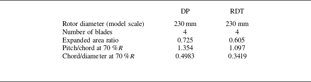


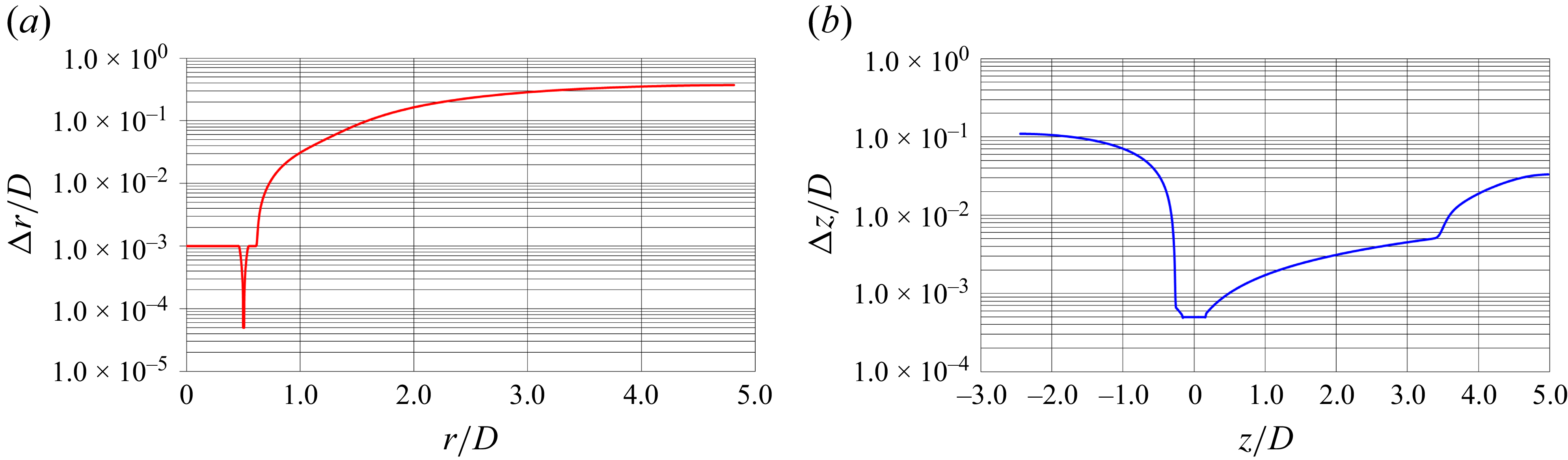


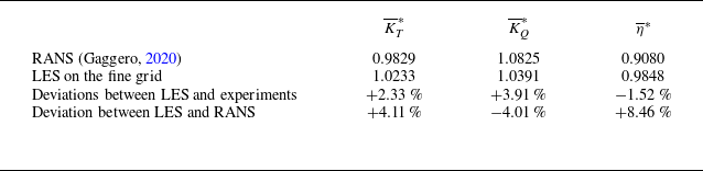

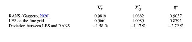

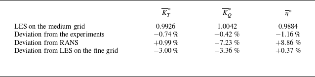

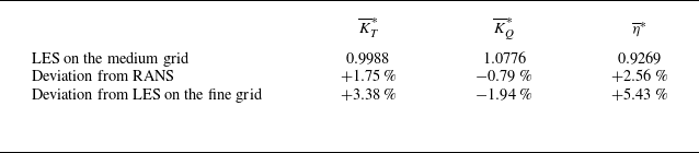

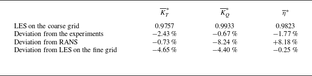

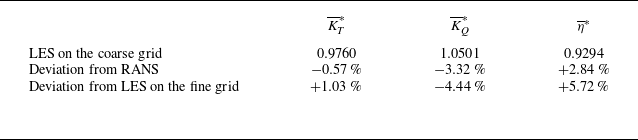


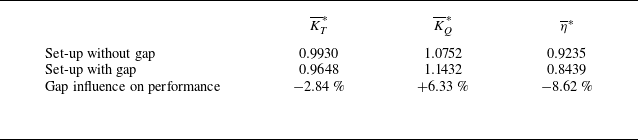


 Open access