





1. Introduction
Capillary or surface-tension-driven phenomena are ubiquitous in nature and various practical applications (Levich Reference Levich1962; Davies & Rideal Reference Davies and Rideal1963; Levich & Krylov Reference Levich and Krylov1969). The emergence of convective motion in a fluid layer induced by an inhomogeneity of a scalar field, such as temperature, solute concentration or electric charge, etc., is known as the Marangoni effect, and the corresponding instability mechanism is referred to as thermocapillary, solutocapillary and electrocapillary, respectively (Scriven & Sternling Reference Scriven and Sternling1960; Davis Reference Davis1987). In various applications related to heat and mass transfer, the surface tension of a fluid depends on the local temperature or/and solute concentration; therefore, understanding the Marangoni instability is crucial for different transport processes. For instance, drying paint (Pearson Reference Pearson1958), flukeprint of a whale (Levy et al. Reference Levy, Uminsky, Park and Calambokidis2011), formation of ripples on the skinned surface of chocolate pudding near the cup centre (Probstein Reference Probstein1994), single crystal growth in a microgravity environment (Schwabe et al. Reference Schwabe, Scharmann, Preisser and Oeder1978), controlling the motion of surface waves (Erinin et al. Reference Erinin, Liu, Liu, Mostert, Deike and Duncan2023), the stability of foams and emulsions (Cohen-Addad, Höhler & Pitois Reference Cohen-Addad, Höhler and Pitois2013; Grassia Reference Grassia2021; Chatzigiannakis et al. Reference Chatzigiannakis, Alicke, Bars, Bidoire and Vermant2025; Sharma et al. Reference Sharma, Borkar, Baumli, Shi, Wu, Myung and Fuller2025) and breakup of a thread (Hameed et al. Reference Hameed, Siegel, Young, Li, Booty and Papageorgiou2008), to mention a few.
At the same time, the Marangoni flow is purposefully employed in various conditions, for example, capillary pumping of pharmaceutical components (Frumkin et al. Reference Frumkin, Mao, Alexeev and Oron2014), suppression of a Rayleigh–Taylor instability (Oron & Rosenau Reference Oron and Rosenau1992; Deissler & Oron Reference Deissler and Oron1992; Burgess et al. Reference Burgess, Juel, McCormick, Swift and Swinney2001; Alexeev & Oron Reference Alexeev and Oron2007), mixing in a low gravity environment, bubble removal in a liquid glass and prevention of radial dopant segregation in semiconductor crystal growth (Ostrach Reference Ostrach1982).
It is known that insoluble and soluble surfactants reduce the surface tension, thereby inducing solutocapillary instability (Palmer & Berg Reference Palmer and Berg1972; Shklyaev & Nepomnyashchy Reference Shklyaev and Nepomnyashchy2013; Morozov, Oron & Nepomnyashchy Reference Morozov, Oron and Nepomnyashchy2014; Guzmán et al. Reference Guzmán, Martínez-Pedrero, Calero, Maestro, Ortega and Rubio2022). However, inorganic ions prefer to remain in the bulk (Oron & Nepomnyashchy Reference Oron and Nepomnyashchy2004); therefore, the solutocapillary effect acts as a stabilising mechanism. On the other hand, colloidal dispersion made of a mixture of base liquid and nanoparticles of diameter $d_p^*\sim 10{-}100$
nm, known as a nanofluid, displays variation of surface tension depending on the interaction between nanoparticle and the liquid–gas interface. For example, a nanofluid consisting of alumina nanoparticles in distilled water exhibits a linear variation of the surface tension with nanoparticle concentration due to the negligible interaction between the nanoparticles and the liquid–gas interface (Gandhi et al. Reference Gandhi, Nepomnyashchy and Oron2025a
,
Reference Gandhi, Nepomnyashchy and Oronc
). However, when nanoparticles are dispersed in different base liquids, such as normal water, ethanol, etc., they start to interact with the liquid–gas interface and become surface active, displaying a non-monotonic variation of the surface tension with nanoparticle concentration (Tanvir & Qiao Reference Tanvir and Qiao2012; Machrafi Reference Machrafi2022).
$d_p^*\sim 10{-}100$
nm, known as a nanofluid, displays variation of surface tension depending on the interaction between nanoparticle and the liquid–gas interface. For example, a nanofluid consisting of alumina nanoparticles in distilled water exhibits a linear variation of the surface tension with nanoparticle concentration due to the negligible interaction between the nanoparticles and the liquid–gas interface (Gandhi et al. Reference Gandhi, Nepomnyashchy and Oron2025a
,
Reference Gandhi, Nepomnyashchy and Oronc
). However, when nanoparticles are dispersed in different base liquids, such as normal water, ethanol, etc., they start to interact with the liquid–gas interface and become surface active, displaying a non-monotonic variation of the surface tension with nanoparticle concentration (Tanvir & Qiao Reference Tanvir and Qiao2012; Machrafi Reference Machrafi2022).
In experimental settings, nanofluids are remarkably engineered to exhibit stable dispersion, so nanoparticles there do not agglomerate. This feature can be achieved using two different approaches: electrostatic stabilisation (Russel, Saville & Schowalter Reference Russel, Saville and Schowalter1989; Russel Reference Russel1991) and steric stabilisation by grafting polymers onto the surface of nanoparticles (Israelachvili Reference Israelachvili2011; van Saarloos, Vitelli & Zeravcic Reference van Saarloos, Vitelli and Zeravcic2023). Therefore, nanofluids considered in the current paper and in Gandhi et al. (Reference Gandhi, Nepomnyashchy and Oron2025c
) are assumed to be preprocessed, so that nanoparticles are sterilised by coating the nanoparticles’ surface with a thin soluble polymer layer of thickness $\approx 2{-}5$
nm (de Kruif et al. Reference de Kruif, van Iersel, Vrij and Russel1985). It is also important to recognise that, depending on the physicochemical properties of the nanoparticles and the electrostatic charge on the solid substrate, particles may irreversibly adsorb on the substrate (Moore, D’Ambrosio & Wray Reference Moore, D’Ambrosio and Wray2025 and references therein). Similarly, it is also possible to adjust the substrate properties to suppress the possibility of irreversible particle adsorption there due to Derjaguin–Landau–Verwey–Overbeek (DLVO) forces (Israelachvili Reference Israelachvili2011; Moraila-Martínez et al. Reference Moraila-Martínez, Cabrerizo-Vílchez and Rodríguez-Valverde2013; Zigelman & Manor Reference Zigelman and Manor2018; Gelderblom, Diddens & Marin Reference Gelderblom, Diddens and Marin2022). In what follows, we neglect particle adsorption at the substrate and focus on the hydrodynamic instabilities driven by surface tension gradients.
$\approx 2{-}5$
nm (de Kruif et al. Reference de Kruif, van Iersel, Vrij and Russel1985). It is also important to recognise that, depending on the physicochemical properties of the nanoparticles and the electrostatic charge on the solid substrate, particles may irreversibly adsorb on the substrate (Moore, D’Ambrosio & Wray Reference Moore, D’Ambrosio and Wray2025 and references therein). Similarly, it is also possible to adjust the substrate properties to suppress the possibility of irreversible particle adsorption there due to Derjaguin–Landau–Verwey–Overbeek (DLVO) forces (Israelachvili Reference Israelachvili2011; Moraila-Martínez et al. Reference Moraila-Martínez, Cabrerizo-Vílchez and Rodríguez-Valverde2013; Zigelman & Manor Reference Zigelman and Manor2018; Gelderblom, Diddens & Marin Reference Gelderblom, Diddens and Marin2022). In what follows, we neglect particle adsorption at the substrate and focus on the hydrodynamic instabilities driven by surface tension gradients.
The thermophysical properties of a nanofluid, such as viscosity, density, heat capacity and thermal conductivity, strongly depend on the local nanoparticle concentration (Buongiorno Reference Buongiorno2006). The density and specific heat capacity of a nanofluid can be fairly reliably taken as a weighted sum of the respective properties, while the viscosity is well approximated with the semi-empirical power-law-type model given by de Kruif et al. (Reference de Kruif, van Iersel, Vrij and Russel1985). Moreover, we note that in shear-induced flows, the normal stress contributions (Phillips et al. Reference Phillips, Armstrong, Brown, Graham and Abbott1992; Lavrenteva, Smagin & Nir Reference Lavrenteva, Smagin and Nir2024) are important in the presence of the base flow; however, in the absence of a base flow, these effects can be safely omitted. Experiments suggest that the thermal conductivity of a nanofluid also depends on the nanoparticle concentration (Pak & Cho Reference Pak and Cho1998). Maxwell (Reference Maxwell1873) and Jeffrey (Reference Jeffrey1973) derived theoretical models for the evaluation of the thermal conductivity of a monodisperse suspension in a dilute limit. Furthermore, Buongiorno (Reference Buongiorno2006) provided an analytical expression as a data fit of the experimental results of Pak & Cho (Reference Pak and Cho1998); henceforth, in our work, we make use of the analytical expression given by Buongiorno (Reference Buongiorno2006).
Due to their excellent thermophysical properties, which can be engineered according to technological requirements, nanofluids are widely used and envisioned in different applications, for example, in heat transfer (Choi & Eastman Reference Choi and Eastman1995), ink jet printing (Lohse Reference Lohse2022), paints, microgravity experiments (Vailati et al. Reference Vailati2023) and nanofluid fuels (Abramzon & Sirignano Reference Abramzon and Sirignano1989; Basu & Miglani Reference Basu and Miglani2016; Vang & Shaw Reference Vang and Shaw2020; Shaw Reference Shaw2022). In a non-isothermal nanofluid layer, the nanoparticles display the mass flux induced by Brownian diffusion given by the generalised Stokes–Einstein formula (Batchelor Reference Batchelor1976; Russel Reference Russel1991) and an additional slip mechanism due to the temperature gradient known as the Soret effect or the thermophoresis effect (Ruckenstein Reference Ruckenstein1981; Anderson Reference Anderson1989; Cross & Hohenberg Reference Cross and Hohenberg1993; Skarda, Jacqmin & McCaughan Reference Skarda, Jacqmin and McCaughan1998).
Recently, Gandhi et al. (Reference Gandhi, Nepomnyashchy and Oron2025a , Reference Gandhi, Nepomnyashchy and Oronc ) developed a general mathematical framework for the thermosolutal instability in a non-isothermal nanofluid layer. They found that, depending on the parameter set, the instability spectrum may vary from the long to short wave. Moreover, the emergence of the instability mechanisms depends on the direction of heating. In binary mixtures, Joo (Reference Joo1995) showed that when a layer of a binary fluid is heated at the liquid–gas interface, the monotonic solutocapillary instability occurs, whereas when it is heated from below, both monotonic and oscillatory thermocapillary instabilities can occur due to the destabilising thermocapillarity and stabilising solutocapillarity. However, for a stratified nanofluid layer, Gandhi et al. (Reference Gandhi, Nepomnyashchy and Oron2025d ) revealed that in the case of a horizontal nanofluid layer heated at the substrate, the solutal buoyancy instability emerges in strong gravity or in a thick layer due to the presence of heavier nanoparticles in the upper stratum of a nanofluid layer.
Stratification of thermophysical properties greatly affects the stability of a system. Variation in thermal conductivity, in particular, imparts subtle changes in the stability properties of stratified fluid systems. Welander (Reference Welander1964) and Welander & Holmåker (Reference Welander and Holmåker1971) found that thermal conductivity stratification destabilises a gravitationally stable system. Additional examples of the role of destabilising thermal conductivity stratification are the classic ‘salt fountain phenomenon’ (Yih Reference Yih1980) and the onset of oscillatory thermocapillary instability with a variation of the thermal conductivity stratification in a nanofluid layer (Gandhi et al. Reference Gandhi, Nepomnyashchy and Oron2025c ).
The theoretical framework for investigating the Marangoni instability in the case of soluble and insoluble surfactants or micelles is well established. Stebe, Lin & Maldarelli (Reference Stebe, Lin and Maldarelli1991) examined both theoretically and experimentally the impact of the interfacial kinetic rate on slug flow in a capillary tube. Shen et al. (Reference Shen, Gleason, McKinley and Stone2002) and Craster, Matar & Papageorgiou (Reference Craster, Matar and Papageorgiou2009) used micelle solutions in applications related to fibre coatings and jet breakup, respectively. Remarkably, Edmonstone, Craster & Matar (Reference Edmonstone, Craster and Matar2006) and Craster & Matar (Reference Craster and Matar2009) studied the pattern formation in a surfactant solution induced by the Marangoni stresses by applying the thin film approximation. Surfactant solutions are often used at a large scale to stabilise foam and as a spreading agent (Edwards, Brenner & Wasan Reference Edwards, Brenner and Wasan1991; Karapetsas, Craster & Matar Reference Karapetsas, Craster and Matar2011). Jensen & Grotberg (Reference Jensen and Grotberg1992) analysed the influence of insoluble surfactant on the liquid–gas interface and the evolution of a thin liquid layer, leading to the layer rupture by the Marangoni flow. Shklyaev & Nepomnyashchy (Reference Shklyaev and Nepomnyashchy2013) and Morozov et al. (Reference Morozov, Oron and Nepomnyashchy2014) investigated the emergence of long-wave thermo-solutocapillary instabilities in the surfactant solution with interfacial kinetics. A recent seminal review article by Manikantan & Squires (Reference Manikantan and Squires2020) presents the intricate role of surface tension-induced hydrodynamic instabilities in complex fluids. However, in the case of colloidal dispersions, models related to surfactants or micelles are not applicable due to the size of the particles (Machrafi Reference Machrafi2022). Additionally, surfactant or micelle solutions, soluble or insoluble, appreciably reduce the surface tension at the liquid–gas interface; however, some nanofluids exhibit a non-monotonic variation of surface tension with the particle concentration.
Following the approach developed in Gandhi et al. (Reference Gandhi, Nepomnyashchy and Oron2025c ) for moderately dense nanofluids, it is assumed that all the thermophysical properties of the nanofluid depend on the local nanoparticle concentration. The purpose of the present paper is to develop a formal theoretical approach and to investigate thermosolutal instability in a moderately dense nanosuspension, taking into account the experimental results of surface tension variation with nanoparticle concentration (Tanvir & Qiao Reference Tanvir and Qiao2012; Harikrishnan et al. Reference Harikrishnan, Dhar, Agnihotri, Gedupudi and Das2017; Machrafi Reference Machrafi2022). The novelty and essence of the present investigation is the inclusion of interfacial nanoparticle adsorption/desorption kinetics into the hydrodynamic model for a nanofluid with the stratification of its thermophysical properties.
The plan of the paper is as follows. Section 2 details the general mathematical formulation of the problem and presents the governing equations and boundary conditions in dimensional and dimensionless forms, taking into account the thermophysical properties of the nanofluid, which depend on the nanoparticle concentration. In addition, in § 2.4, a quiescent base state of the system is derived. Section 3 introduces the framework for the linear stability analysis of the base state of the system and presents the linear eigenvalue problem (EVP) in terms of normal-form perturbations. Section 3.1 briefly describes the numerical procedure and introduces further simplifications to the EVP, before the numerical solution is performed. Section 4 presents the results and their discussion for various cases. Section 4.3 presents the analytical solution for the simplified toy problem, whose aim is to pinpoint the important instability mechanisms in a similar physical system, focusing on the roles of thermal conductivity stratification and interfacial kinetics. Section 5 summarises the findings of the present paper. Appendix A provides, based on the total interaction potential, further details on the estimation of the rates of interfacial kinetics. Furthermore, Appendix B contains the details of the linear stability analysis of the toy problem presented in § 4.3. Finally, in Appendix C, we provide the validation of the numerical approach versus the analytical result obtained in Appendix B.
2. Problem formulation
We consider a nanofluid layer of a mean thickness $h_0^\ast$
with density
$h_0^\ast$
with density $\rho ^\ast _{\textit{nf}}$
, dynamic viscosity
$\rho ^\ast _{\textit{nf}}$
, dynamic viscosity $\mu ^\ast _{\textit{nf}}$
, kinematic viscosity
$\mu ^\ast _{\textit{nf}}$
, kinematic viscosity $\nu ^\ast _{\textit{nf}}=\mu ^\ast _{\textit{nf}}/\rho ^\ast _{\textit{nf}}$
, thermal conductivity
$\nu ^\ast _{\textit{nf}}=\mu ^\ast _{\textit{nf}}/\rho ^\ast _{\textit{nf}}$
, thermal conductivity $K^\ast _{\textit{nf}}$
, heat capacity
$K^\ast _{\textit{nf}}$
, heat capacity $c^\ast _{\textit{nf}}$
and thermal diffusivity
$c^\ast _{\textit{nf}}$
and thermal diffusivity $\kappa ^\ast _{\textit{nf}} = K^\ast _{\textit{nf}}/\rho ^\ast _{\textit{nf}} c^\ast _{\textit{nf}}$
. Hereon, we denote the thermophysical properties of a nanofluid, a base fluid and nanoparticles with the subscripts
$\kappa ^\ast _{\textit{nf}} = K^\ast _{\textit{nf}}/\rho ^\ast _{\textit{nf}} c^\ast _{\textit{nf}}$
. Hereon, we denote the thermophysical properties of a nanofluid, a base fluid and nanoparticles with the subscripts $nf$
,
$nf$
, $bf$
and
$bf$
and $np$
, respectively. The nanofluid layer with local instantaneous thickness
$np$
, respectively. The nanofluid layer with local instantaneous thickness $h^*(x^*,y^*,t^*)$
is deposited on the rigid and impermeable horizontal substrate and exposed to the quiescent gas environment held at constant pressure
$h^*(x^*,y^*,t^*)$
is deposited on the rigid and impermeable horizontal substrate and exposed to the quiescent gas environment held at constant pressure $p^\ast _\infty$
and temperature
$p^\ast _\infty$
and temperature $T_\infty ^*$
in the gravity field
$T_\infty ^*$
in the gravity field $g^*$
. The chosen frame of reference is that the
$g^*$
. The chosen frame of reference is that the $x^\ast$
and
$x^\ast$
and $y^\ast$
axes are located on the substrate, whereas the
$y^\ast$
axes are located on the substrate, whereas the $z^\ast$
axis is normal to the substrate and directed into the fluid layer in the direction opposite to that of gravity, therefore, the substrate and the deformable liquid–gas interface are located at
$z^\ast$
axis is normal to the substrate and directed into the fluid layer in the direction opposite to that of gravity, therefore, the substrate and the deformable liquid–gas interface are located at $z^\ast =0$
and
$z^\ast =0$
and $z^\ast =h^\ast (x^*,y^*,t^*)$
at time
$z^\ast =h^\ast (x^*,y^*,t^*)$
at time $t^\ast$
, respectively, as shown in figure 1.
$t^\ast$
, respectively, as shown in figure 1.
The nanofluid layer is assumed to be moderately dense in terms of the volumetric nanoparticle concentration $\phi ^\ast = \phi ^\ast (x^\ast ,y^\ast ,z^\ast ,t^\ast )$
that varies in space
$\phi ^\ast = \phi ^\ast (x^\ast ,y^\ast ,z^\ast ,t^\ast )$
that varies in space $(x^\ast ,y^\ast ,z^\ast )$
and time
$(x^\ast ,y^\ast ,z^\ast )$
and time $t^*$
. We note that the terminology ‘moderately dense’ is used here and in our previous papers (Gandhi et al. Reference Gandhi, Nepomnyashchy and Oron2025a
,Reference Gandhi, Nepomnyashchy and Oron
b
,Reference Gandhi, Nepomnyashchy and Oron
c
) for nanofluids to indicate that the thermophysical properties are no longer constant, as in the case of dilute binary mixtures. Instead, the particle concentration is still low,
$t^*$
. We note that the terminology ‘moderately dense’ is used here and in our previous papers (Gandhi et al. Reference Gandhi, Nepomnyashchy and Oron2025a
,Reference Gandhi, Nepomnyashchy and Oron
b
,Reference Gandhi, Nepomnyashchy and Oron
c
) for nanofluids to indicate that the thermophysical properties are no longer constant, as in the case of dilute binary mixtures. Instead, the particle concentration is still low, $\phi ^*\ll 1$
, but sufficiently high, so that the leading-order contribution
$\phi ^*\ll 1$
, but sufficiently high, so that the leading-order contribution $O(\phi ^*)$
for the thermophysical properties of the nanofluid is important and can not be ignored beforehand. The hard spherical particles with diameter
$O(\phi ^*)$
for the thermophysical properties of the nanofluid is important and can not be ignored beforehand. The hard spherical particles with diameter $d_p^*\approx 50$
nm are suspended in a layer of a Newtonian carrier fluid. In addition, we note that an inherent nanoparticle interaction with the surrounding gas phase mediated by a carrier liquid leads to nanoparticle adsorption and desorption at/from the air–liquid interface, where the interfacial nanoparticle concentration is denoted
$d_p^*\approx 50$
nm are suspended in a layer of a Newtonian carrier fluid. In addition, we note that an inherent nanoparticle interaction with the surrounding gas phase mediated by a carrier liquid leads to nanoparticle adsorption and desorption at/from the air–liquid interface, where the interfacial nanoparticle concentration is denoted $\varGamma ^*(x^*,y^*,t^*)$
(Machrafi Reference Machrafi2022). The lateral interaction of nanoparticles at the interface will be neglected; hence, the influence is limited to the effects of vertical interfacial kinetics only. The nanofluid layer is assumed to be cooled at its solid bottom with the prescribed heat flux
$\varGamma ^*(x^*,y^*,t^*)$
(Machrafi Reference Machrafi2022). The lateral interaction of nanoparticles at the interface will be neglected; hence, the influence is limited to the effects of vertical interfacial kinetics only. The nanofluid layer is assumed to be cooled at its solid bottom with the prescribed heat flux $-q^\ast ,\,q^\ast \gt 0$
in the vertical direction. An imposed heat flux leads to the emergence of the temperature field
$-q^\ast ,\,q^\ast \gt 0$
in the vertical direction. An imposed heat flux leads to the emergence of the temperature field $T^\ast =T^\ast (x^\ast ,y^\ast ,z^\ast ,t^\ast )$
that varies with time and space within the layer.
$T^\ast =T^\ast (x^\ast ,y^\ast ,z^\ast ,t^\ast )$
that varies with time and space within the layer.
2.1. Thermophysical properties and physical mechanisms
The thermophysical properties of a nanofluid exhibit a strong dependence on the local nanoparticle concentration (Buongiorno Reference Buongiorno2006). We consider the density and specific heat of a nanofluid layer as a weighted sum of the respective properties, with the particle volume fraction as a weight
 \begin{equation} \rho ^\ast _{\textit{nf}}(\phi ^\ast ) =(1-\phi ^\ast )\rho ^\ast _{\textit{bf}}+\phi ^\ast \rho ^\ast _{\textit{np}},\quad c^\ast _{\textit{nf}}(\phi ^\ast ) = \frac {(1-\phi ^\ast )(\rho ^\ast c^\ast ) _{\textit{bf}}+ \phi ^\ast (\rho ^\ast c^\ast ) _{\textit{np}}}{\rho _{\textit{nf}}^\ast }. \end{equation}
Nanofluid layer with particles of diameter $d_p^* \sim 50 \,\text{nm}$
deposited on the solid substrate, subjected to a constant heat flux at the substrate and exposed to the gas phase at its deformable interface with interfacial adsorption/desorption particle kinetics.
$d_p^* \sim 50 \,\text{nm}$
deposited on the solid substrate, subjected to a constant heat flux at the substrate and exposed to the gas phase at its deformable interface with interfacial adsorption/desorption particle kinetics.

Pak & Cho (Reference Pak and Cho1998), Buongiorno et al. (Reference Buongiorno2009) and Keblinski, Prasher & Eapen (Reference Keblinski, Prasher and Eapen2008) showed experimentally a significant enhancement of thermal conductivity with the Al $_2$
O
$_2$
O $_3$
nanoparticles in water as a base liquid. Buongiorno (Reference Buongiorno2006) suggested the empirical linear fit for the thermal conductivity variation with local nanoparticle concentration, which is valid for a moderately dense nanofluid. This empirical model for the thermal conductivity reads
$_3$
nanoparticles in water as a base liquid. Buongiorno (Reference Buongiorno2006) suggested the empirical linear fit for the thermal conductivity variation with local nanoparticle concentration, which is valid for a moderately dense nanofluid. This empirical model for the thermal conductivity reads
 \begin{equation} K^\ast _{\textit{nf}}(\phi ^\ast ) = K^\ast _{\textit{bf}}(1 + a \phi ^\ast ), \end{equation}
where $K_{\textit{bf}}^*$
is the thermal conductivity of the base fluid and the parameter
$K_{\textit{bf}}^*$
is the thermal conductivity of the base fluid and the parameter $a$
represents the strength of variation of the thermal conductivity with the local nanoparticle concentration
$a$
represents the strength of variation of the thermal conductivity with the local nanoparticle concentration $\phi ^\ast$
. We note that the thermal conductivity model given by (2.2) is similar in its form to the classical model given by Maxwell (Reference Maxwell1873) in the limit of a dilute suspension of monodispersed hard spheres in a single-component liquid. Jeffrey (Reference Jeffrey1973) extended the model for the case of the thermal conductivity of a suspension of Maxwell (Reference Maxwell1873) valid up to
$\phi ^\ast$
. We note that the thermal conductivity model given by (2.2) is similar in its form to the classical model given by Maxwell (Reference Maxwell1873) in the limit of a dilute suspension of monodispersed hard spheres in a single-component liquid. Jeffrey (Reference Jeffrey1973) extended the model for the case of the thermal conductivity of a suspension of Maxwell (Reference Maxwell1873) valid up to $O(\phi ^*)$
to the higher order in local nanoparticle concentration
$O(\phi ^*)$
to the higher order in local nanoparticle concentration $O(\phi ^{*2})$
. The empirical fit given by Buongiorno (Reference Buongiorno2006) for the experiments of Pak & Cho (Reference Pak and Cho1998) in the case of alumina nanoparticles in water leads to the value of the parameter
$O(\phi ^{*2})$
. The empirical fit given by Buongiorno (Reference Buongiorno2006) for the experiments of Pak & Cho (Reference Pak and Cho1998) in the case of alumina nanoparticles in water leads to the value of the parameter $a = 7.47$
, on the other hand, the corresponding value of
$a = 7.47$
, on the other hand, the corresponding value of $a$
obtained from the Maxwell (Reference Maxwell1873) model yields
$a$
obtained from the Maxwell (Reference Maxwell1873) model yields $a \leqslant 3$
, which is quite far from the experimental value
$a \leqslant 3$
, which is quite far from the experimental value $a=7.47$
. This difference could be associated with the possibility of the formation of aggregates. In what follows, we use the value
$a=7.47$
. This difference could be associated with the possibility of the formation of aggregates. In what follows, we use the value $a=7.47$
. In addition, it is possible to estimate the value of the thermal conductivity variation via the Hashin–Shtrikman bounds (Hashin & Shtrikman Reference Hashin and Shtrikman1962; Keblinski et al. Reference Keblinski, Prasher and Eapen2008)
$a=7.47$
. In addition, it is possible to estimate the value of the thermal conductivity variation via the Hashin–Shtrikman bounds (Hashin & Shtrikman Reference Hashin and Shtrikman1962; Keblinski et al. Reference Keblinski, Prasher and Eapen2008)
 \begin{equation} \left [1+\frac {3\phi ^* \big (K_{\textit{np}}^*-K_{\textit{bf}}^*\big )}{3K_{\textit{bf}}^*+\left (1-\phi ^*\right )\big (K_{\textit{np}}^*-K_{\textit{bf}}^*\big )}\right ]\leqslant \frac {K_{\textit{nf}}^*}{K_{\textit{bf}}^*}\leqslant \left [1-\frac {3(1-\phi ^*)\big (K_{\textit{np}}^*-K_{\textit{bf}}^*\big )}{3K_{\textit{np}}^*-\phi ^*\big (K_{\textit{np}}^*-K_{\textit{bf}}^*\big )}\right ]\frac {K_{\textit{np}}^*}{K_{\textit{bf}}^*}. \end{equation}
For the low nanoparticle concentration limit, $\phi ^*\ll 1$
, the thermal conductivity parameter
$\phi ^*\ll 1$
, the thermal conductivity parameter $a$
for the Al
$a$
for the Al $_2$
O
$_2$
O $_3$
nanoparticles in water ranges in the interval
$_3$
nanoparticles in water ranges in the interval $2.84\le a\le 38$
, so the value
$2.84\le a\le 38$
, so the value $a=7.47$
belongs to this interval.
$a=7.47$
belongs to this interval.
For the nanofluid viscosity, we use the model suggested by de Kruif et al. (Reference de Kruif, van Iersel, Vrij and Russel1985) for the hard-sphere nanoparticle suspension in an electrostatically stabilised base liquid, i.e.
 \begin{equation} \mu ^\ast _{\textit{nf}}(\phi ^\ast ) = \mu ^\ast _{\textit{bf}} \left (1-\frac {\phi ^\ast }{\phi _m}\right )^{-2}, \end{equation}
where $\phi _m$
stands for random close packing. The values of
$\phi _m$
stands for random close packing. The values of $\phi _m$
vary in the interval between
$\phi _m$
vary in the interval between $0.524-0.71$
. We use the value
$0.524-0.71$
. We use the value $\phi _m=0.65$
satisfying the experimental observations of de Kruif et al. (Reference de Kruif, van Iersel, Vrij and Russel1985) for the zero-shear limit.
$\phi _m=0.65$
satisfying the experimental observations of de Kruif et al. (Reference de Kruif, van Iersel, Vrij and Russel1985) for the zero-shear limit.
The absolute velocity of a nanoparticle is described by the sum of the carrier fluid velocity and the relative (slip) velocity. Buongiorno (Reference Buongiorno2006) describes seven different slip mechanisms for a nanofluid suspension, which are inertia, Brownian diffusion, thermophoresis or the Soret effect, diffusiophoresis, Magnus effect, fluid drainage and gravitational settling. Out of these seven, we consider the two dominant slip mechanisms, i.e. Brownian diffusion and the Soret effect.
The Brownian diffusivity is determined from the Stokes–Einstein formula, i.e.
 \begin{equation} D_B = \frac {K_B^*T^\ast }{3\pi \mu ^\ast _{\textit{bf}}d_p^\ast }, \end{equation}
where $K_B^*$
is the Boltzmann constant,
$K_B^*$
is the Boltzmann constant, $K_B^*= 1.380649 \times 10^{-23}$
J/K. We note that Brownian diffusivity also depends on the nanoparticle concentration (Batchelor Reference Batchelor1976; Russel et al. Reference Russel, Saville and Schowalter1989; Bird, Stewart & Lightfoot Reference Bird, Stewart and Lightfoot2002); however, for a low particle concentration, the particle concentration-dependent Brownian diffusivity imparts negligible influence on the stability (Gandhi et al. Reference Gandhi, Nepomnyashchy and Oron2025c
); therefore, in this condition, the constant Brownian diffusivity provides a good approximation.
$K_B^*= 1.380649 \times 10^{-23}$
J/K. We note that Brownian diffusivity also depends on the nanoparticle concentration (Batchelor Reference Batchelor1976; Russel et al. Reference Russel, Saville and Schowalter1989; Bird, Stewart & Lightfoot Reference Bird, Stewart and Lightfoot2002); however, for a low particle concentration, the particle concentration-dependent Brownian diffusivity imparts negligible influence on the stability (Gandhi et al. Reference Gandhi, Nepomnyashchy and Oron2025c
); therefore, in this condition, the constant Brownian diffusivity provides a good approximation.
In a non-isothermal nanofluid layer, the temperature gradient induced between the solid substrate and the deformable interface can induce another slip mechanism known as thermophoresis that is similar to the Soret effect in the kinetic theory of gases. We assume the Soret effect for the single-component nanofluid mixture given by (Whitmore & Meisen Reference Whitmore and Meisen1977; Buongiorno Reference Buongiorno2006)
 \begin{equation} D_T = \left (\frac {0.26K^\ast _{\textit{bf}}}{2K^\ast _{\textit{bf}}+K^\ast _{\textit{np}}}\right )\frac {\mu ^\ast _{\textit{bf}}}{\rho ^\ast _{\textit{bf}}}\phi ^\ast . \end{equation}
Thence, the total nanoparticle mass flux is expressed by the mass flux induced by the Brownian diffusion and the Soret effect as
 \begin{equation} \boldsymbol{j}_p = -\rho ^\ast _{\textit{np}}\left ( C_BT^\ast \boldsymbol{\nabla} ^\ast \phi ^\ast + C_T\phi ^\ast \frac {\boldsymbol{\nabla} ^\ast T^\ast }{T^\ast }\right ), \end{equation}
where $C_B = D_B/T^\ast$
,
$C_B = D_B/T^\ast$
, $C_T = D_T/\phi ^\ast $
and
$C_T = D_T/\phi ^\ast $
and $\displaystyle \boldsymbol{\nabla} ^\ast = (\partial _{x^\ast }, \partial _{y^\ast },\partial _{z^\ast } )$
, with subscripts
$\displaystyle \boldsymbol{\nabla} ^\ast = (\partial _{x^\ast }, \partial _{y^\ast },\partial _{z^\ast } )$
, with subscripts ${x^\ast }, {y^\ast },{z^\ast }$
representing partial differentiation with respect to the corresponding variable. We note in passing that the total mass flux of nanoparticles given by (2.7) ensures a positively definite distribution of nanoparticle concentration, even subjected to strong thermophoresis. The other five slip mechanisms are negligible for a thin nanofluid layer with the diameter
${x^\ast }, {y^\ast },{z^\ast }$
representing partial differentiation with respect to the corresponding variable. We note in passing that the total mass flux of nanoparticles given by (2.7) ensures a positively definite distribution of nanoparticle concentration, even subjected to strong thermophoresis. The other five slip mechanisms are negligible for a thin nanofluid layer with the diameter $d_p^*=50$
nm; however, the gravitational setting becomes important for the thick layer or in suspensions with larger nanoparticles (Chang & Ruo Reference Chang and Ruo2022; Gandhi et al. Reference Gandhi, Nepomnyashchy and Oron2025c
).
$d_p^*=50$
nm; however, the gravitational setting becomes important for the thick layer or in suspensions with larger nanoparticles (Chang & Ruo Reference Chang and Ruo2022; Gandhi et al. Reference Gandhi, Nepomnyashchy and Oron2025c
).
We assume that the heat flux in a nanofluid is given by the Fourier’s law of heat conduction, i.e.
 \begin{equation} \boldsymbol{j}_T = - K_{\textit{nf}}^\ast \boldsymbol{\nabla} ^\ast T^\ast , \end{equation}
where we neglect the heat transfer contribution due to the Dufour effect and the nanoparticle mass transfer. The Dufour effect is negligible for the liquid mixture (Cross & Hohenberg Reference Cross and Hohenberg1993; Oron & Nepomnyashchy Reference Oron and Nepomnyashchy2004); however, important for the heat transfer in gases. We note that other components of the mass flux of nanoparticles (Buongiorno Reference Buongiorno2006), such as sedimentation (Chang & Ruo Reference Chang and Ruo2022), can also contribute to the total heat flux. However, in the case of a thin nanofluid layer with small-sized nanoparticles, they are negligible (Gandhi et al. Reference Gandhi, Nepomnyashchy and Oron2025c ).
2.2. Governing equations and boundary conditions
The set of governing equations describing the dynamics of a nanofluid layer contains the continuity, Navier–Stokes, advection–conduction heat transfer and particle mass transfer equations, respectively (Rohsenow, Hartnett & Cho Reference Rohsenow, Hartnett and Cho1998; Batchelor Reference Batchelor2000; Colinet, Legros & Velarde Reference Colinet, Legros and Velarde2001; Bird et al. Reference Bird, Stewart and Lightfoot2002):
 \begin{align} \big(\rho _{\textit{nf}}^*\big)_{t^*} + \boldsymbol{\nabla} ^\ast & \boldsymbol{\cdot }\big(\rho _{\textit{nf}}^*\boldsymbol{u}^*\big) = 0, \end{align}
 \begin{align} \big(\rho _{\textit{nf}}^*\boldsymbol{u}^*\big)_{t^*} + \boldsymbol{\nabla} ^\ast \boldsymbol{\cdot }\big(\rho _{\textit{nf}}^*\boldsymbol{u}^*\boldsymbol{u}^*\big) &= -\boldsymbol{\nabla} ^\ast p^* + \boldsymbol{\nabla} ^\ast \boldsymbol{\cdot }\boldsymbol{\tau }^* -\rho _{\textit{nf}}^*g^*\boldsymbol{e}_{z^*}, \end{align}
 \begin{align} \big(\rho ^* c^*\big)_{\textit{nf}}T^*_{t^*} + \big(\rho ^* c^*\big)_{\textit{nf}} \big(\boldsymbol{u}^\ast \boldsymbol{\cdot }\boldsymbol{\nabla} ^\ast \big) T^\ast &= \boldsymbol{\nabla} ^\ast \boldsymbol{\cdot }\big(K_{\textit{nf}}^*\boldsymbol{\nabla} ^\ast T^*\big), \end{align}
 \begin{align} \phi ^*_{t^*} + \boldsymbol{\nabla} ^\ast \boldsymbol{\cdot }\big(\boldsymbol{u}^*\phi ^*\big) &= \boldsymbol{\nabla} ^\ast \boldsymbol{\cdot }\biggl (C_BT^*\boldsymbol{\nabla} ^\ast \phi ^* +C_T\phi ^*\frac {\boldsymbol{\nabla} ^\ast T^*}{T^*}\biggr ). \end{align}
Here, $g^*$
is the gravity acceleration,
$g^*$
is the gravity acceleration, $\boldsymbol{e}_{z^*}$
is the unit vector in the
$\boldsymbol{e}_{z^*}$
is the unit vector in the $z^\ast$
direction,
$z^\ast$
direction, ${\boldsymbol u}^* = (u^*,v^*,w^* )$
is the flow velocity field vector and
${\boldsymbol u}^* = (u^*,v^*,w^* )$
is the flow velocity field vector and $\boldsymbol{\tau }^*$
is the viscous part of the stress tensor
$\boldsymbol{\tau }^*$
is the viscous part of the stress tensor $\displaystyle \boldsymbol{\tau }^* =\mu _{\textit{nf}}^\ast [\boldsymbol{\nabla} ^\ast {\boldsymbol u^*}+ (\boldsymbol{\nabla} ^\ast {\boldsymbol u^*} )^\intercal ] - ({2}/{3}\mu _{\textit{nf}}^\ast - \mathcal{K}^\ast ) (\boldsymbol{\nabla} ^\ast \boldsymbol{\cdot }\boldsymbol{u}^\ast ) \boldsymbol{I}$
, where the superscript
$\displaystyle \boldsymbol{\tau }^* =\mu _{\textit{nf}}^\ast [\boldsymbol{\nabla} ^\ast {\boldsymbol u^*}+ (\boldsymbol{\nabla} ^\ast {\boldsymbol u^*} )^\intercal ] - ({2}/{3}\mu _{\textit{nf}}^\ast - \mathcal{K}^\ast ) (\boldsymbol{\nabla} ^\ast \boldsymbol{\cdot }\boldsymbol{u}^\ast ) \boldsymbol{I}$
, where the superscript $^\intercal$
denotes the transpose of the corresponding tensor,
$^\intercal$
denotes the transpose of the corresponding tensor, $\boldsymbol{I}$
is the unity tensor, the subscript
$\boldsymbol{I}$
is the unity tensor, the subscript $t^\ast$
stands for a partial derivative with respect to time
$t^\ast$
stands for a partial derivative with respect to time $t^\ast$
and
$t^\ast$
and $\mathcal{K}^\ast$
is the dilatational viscosity of the fluid. We note that the last term in (2.9b
) represents the buoyancy force, which is due to the fluid density varying within the layer with the particle concentration that is, in turn, coupled to the fluid temperature via the governing equations (2.9).
$\mathcal{K}^\ast$
is the dilatational viscosity of the fluid. We note that the last term in (2.9b
) represents the buoyancy force, which is due to the fluid density varying within the layer with the particle concentration that is, in turn, coupled to the fluid temperature via the governing equations (2.9).
We impose three boundary conditions at the solid–liquid interface $z^*=0$
. The boundary conditions at the solid substrate are
$z^*=0$
. The boundary conditions at the solid substrate are
 \begin{equation} z^\ast =0: \quad \boldsymbol{u}^* = 0, \quad -K_{\textit{nf}}^{*}T^*_{z^\ast } = -q^*, \quad C_BT^* \phi ^*_{z^\ast }+C_T\phi ^*\frac {T^*_{z^\ast }}{T^*} = 0. \end{equation}
The first condition represents the no-slip and no-penetration for the flow velocity at the substrate. The second condition describes the heat transfer to the solid substrate made of a material with a low thermal conductivity, which is represented by a specified heat flux $-q^*$
(Rohsenow et al. Reference Rohsenow, Hartnett and Cho1998). Finally, the third condition corresponds to the impermeability of the substrate in terms of the total mass flux of the nanoparticles.
$-q^*$
(Rohsenow et al. Reference Rohsenow, Hartnett and Cho1998). Finally, the third condition corresponds to the impermeability of the substrate in terms of the total mass flux of the nanoparticles.
In what follows, we consider the deformable liquid–air interface exposed to the gas phase in the gravity field. The motion of the interface located at $z^*=h^*(x^*,y^*,t^*)$
is governed by the kinematic boundary condition
$z^*=h^*(x^*,y^*,t^*)$
is governed by the kinematic boundary condition
 \begin{equation} h_{t^*}^*+u^*h_{x^*}^*+v^*h_{y^*}^*=w^*. \end{equation}
The next boundary condition at the deformable interface $z^* = h^*(x^*,y^*,t^*)$
is the continuity of the normal and tangential stresses
$z^* = h^*(x^*,y^*,t^*)$
is the continuity of the normal and tangential stresses
 \begin{equation} \boldsymbol{n}^\ast \boldsymbol{\cdot }\boldsymbol{\mathcal{T}}^*\boldsymbol{\cdot }\boldsymbol{n}^\ast = 2\boldsymbol{\mathcal{H}}^\ast \sigma ^\ast ,\quad \boldsymbol{n}^\ast \boldsymbol{\cdot }\boldsymbol{\mathcal{T}}^*\boldsymbol{\cdot }\boldsymbol{x}^\ast = \boldsymbol{x}^\ast \boldsymbol{\cdot }\boldsymbol{\nabla} ^\ast _s\sigma ^*,\quad \boldsymbol{n}^\ast \boldsymbol{\cdot }\boldsymbol{\mathcal{T}}^*\boldsymbol{\cdot }\boldsymbol{y}^\ast = \boldsymbol{y}^\ast \boldsymbol{\cdot }\boldsymbol{\nabla} ^\ast _s\sigma ^*, \end{equation}
where $\boldsymbol{\mathcal{T}}^*= -p^*\boldsymbol{I} + \boldsymbol{\tau }^\ast$
is the total stress tensor. Here,
$\boldsymbol{\mathcal{T}}^*= -p^*\boldsymbol{I} + \boldsymbol{\tau }^\ast$
is the total stress tensor. Here, $\displaystyle \boldsymbol{\nabla} ^\ast _s = (\boldsymbol{I} - \boldsymbol{n}^\ast \boldsymbol{n}^\ast )\boldsymbol{\cdot }\boldsymbol{\nabla} ^\ast$
is the surface gradient operator,
$\displaystyle \boldsymbol{\nabla} ^\ast _s = (\boldsymbol{I} - \boldsymbol{n}^\ast \boldsymbol{n}^\ast )\boldsymbol{\cdot }\boldsymbol{\nabla} ^\ast$
is the surface gradient operator,
 \begin{equation} \boldsymbol{n}^\ast = \frac {-h_{x^*}^*\boldsymbol{e}_{x^*}-h_{y^*}^*\boldsymbol{e}_{y^*}+\boldsymbol{e}_{z^*}}{\sqrt {1+h_{x^*}^{*2}+h_{y^*}^{*2}}} \end{equation}
is the unit vector normal to the interface, $\boldsymbol{e}_{x^\ast }$
and
$\boldsymbol{e}_{x^\ast }$
and $\boldsymbol{e}_{y^\ast }$
are the orthonormal vectors in the
$\boldsymbol{e}_{y^\ast }$
are the orthonormal vectors in the $x^\ast$
and
$x^\ast$
and $y^\ast$
directions, respectively,
$y^\ast$
directions, respectively,
 \begin{equation} \boldsymbol{x}^\ast = \frac {\boldsymbol{e}_{x^*}+h_{x^*}^*\boldsymbol{e}_{z^*}}{\sqrt {1+h_{x^*}^{*2}}},\qquad \boldsymbol{y}^\ast =\frac {\boldsymbol{e}_{y^*}+h_{y^*}^*\boldsymbol{e}_{z^*}}{\sqrt {1+h_{y^*}^{*2}}}, \end{equation}
are unit vectors tangent to the interface and $2\boldsymbol{\mathcal{H}}^*$
is the mean curvature of the interface
$2\boldsymbol{\mathcal{H}}^*$
is the mean curvature of the interface
 \begin{equation} 2\boldsymbol{\mathcal{H}}^* = -\boldsymbol{\nabla} ^\ast _s\boldsymbol{\cdot }\boldsymbol{n}^\ast . \end{equation}
Henceforth, following Stokes’ hypothesis (Buresti Reference Buresti2015), we assume a zero value of the dilatational viscosity $\mathcal{K}^\ast$
. This signifies that the absolute value of
$\mathcal{K}^\ast$
. This signifies that the absolute value of $\displaystyle \mathcal{K}^\ast \boldsymbol{\nabla} ^\ast \boldsymbol{\cdot }\boldsymbol{u}^\ast$
is negligible compared with the thermodynamic pressure
$\displaystyle \mathcal{K}^\ast \boldsymbol{\nabla} ^\ast \boldsymbol{\cdot }\boldsymbol{u}^\ast$
is negligible compared with the thermodynamic pressure $p^\ast$
, i.e.
$p^\ast$
, i.e. $\displaystyle |\mathcal{K}^\ast \boldsymbol{\nabla} ^\ast \boldsymbol{\cdot }\boldsymbol{u}^\ast |\ll p^\ast$
. We note that the value of the surface tension
$\displaystyle |\mathcal{K}^\ast \boldsymbol{\nabla} ^\ast \boldsymbol{\cdot }\boldsymbol{u}^\ast |\ll p^\ast$
. We note that the value of the surface tension $\sigma ^\ast$
will be derived in (2.25).
$\sigma ^\ast$
will be derived in (2.25).
The heat transfer boundary condition at the interface $z^*=h^*(x^*,y^*,t^*)$
is expressed by Newton’s law of cooling
$z^*=h^*(x^*,y^*,t^*)$
is expressed by Newton’s law of cooling
 \begin{equation} -K_{\textit{nf}}^*\boldsymbol{\nabla} ^\ast T^*\boldsymbol{\cdot }\boldsymbol{n}^\ast =\widehat {q}(T^*-T_\infty ^*), \end{equation}
where $\widehat {q}$
is the rate of heat transfer from the liquid to gas phase by convection. This boundary condition effectively couples the temperature and local particle concentration at the interface since
$\widehat {q}$
is the rate of heat transfer from the liquid to gas phase by convection. This boundary condition effectively couples the temperature and local particle concentration at the interface since $K_{\textit{nf}}^\ast$
depends on the latter.
$K_{\textit{nf}}^\ast$
depends on the latter.
Additionally, at the liquid–air interface, the interfacial concentration $\varGamma ^\ast$
defined hereon in units of mol m
$\varGamma ^\ast$
defined hereon in units of mol m $^{-2}$
is given by (Machrafi Reference Machrafi2022)
$^{-2}$
is given by (Machrafi Reference Machrafi2022)
 \begin{equation} \varGamma ^* = \vartheta \,\varGamma ^*_\infty , \end{equation}
where $\vartheta$
and
$\vartheta$
and $\displaystyle {\varGamma ^*_\infty = \vartheta _\infty \mathcal{L}_{\textit{np}}^*({\rho _{\textit{np}}^*}/{\mathcal{M}_{\textit{np}}^*}})$
are the surface coverage and the maximum surface concentration in units of mol m
$\displaystyle {\varGamma ^*_\infty = \vartheta _\infty \mathcal{L}_{\textit{np}}^*({\rho _{\textit{np}}^*}/{\mathcal{M}_{\textit{np}}^*}})$
are the surface coverage and the maximum surface concentration in units of mol m $^{-2}$
, respectively. For spherical particles, the maximum geometrical coverage fraction
$^{-2}$
, respectively. For spherical particles, the maximum geometrical coverage fraction $\vartheta _\infty = 0.547$
, the characteristic length
$\vartheta _\infty = 0.547$
, the characteristic length $\mathcal{L}^*_{\textit{np}} = d_p^*/3$
and the factor
$\mathcal{L}^*_{\textit{np}} = d_p^*/3$
and the factor
 \begin{equation} \frac {\rho _{\textit{np}}^*}{\mathcal{M}_{\textit{np}}^*} = \left [\frac {4\pi ^2}{9\sqrt {2}}\left (\frac {d_p^*}{2}\right )^3N_A^*\right ]^{-1} \end{equation}
yields an equivalent bulk nanoparticle concentration volume fraction to the interfacial molar mass, in units of mol m $^{-3}$
, where
$^{-3}$
, where $N_A^* = 6.02\times 10^{23}$
mol
$N_A^* = 6.02\times 10^{23}$
mol $^{-1}$
is Avogadro’s number. Note that nanoparticles are neither molecules nor atoms, yet they are treated as a polymer made of many monomers, a collection of chemically connected atoms or molecules. In what follows, the molar mass of a nanoparticle is given by (Machrafi Reference Machrafi2022)
$^{-1}$
is Avogadro’s number. Note that nanoparticles are neither molecules nor atoms, yet they are treated as a polymer made of many monomers, a collection of chemically connected atoms or molecules. In what follows, the molar mass of a nanoparticle is given by (Machrafi Reference Machrafi2022)
 \begin{equation} \mathcal{M}_{\textit{np}}^* = \mathcal{M}_{\textit{np}}^{*\prime }f_{\textit{np}}\frac {\mathcal{V}_{\textit{np}}^*}{\mathcal{V}_{\textit{np}}^{*\prime }}, \end{equation}
where $\mathcal{M}_{\textit{np}}^{*\prime }$
and
$\mathcal{M}_{\textit{np}}^{*\prime }$
and $\displaystyle {f_{\textit{np}} = {\pi }/{3\sqrt {2}}}$
represent the molar mass of one molecule and maximum three-dimensional nanoparticle packing density, e.g. face-centred cubic of spheres, respectively. Furthermore, the volumes of a nanoparticle and a spherical molecule are defined, respectively, as
$\displaystyle {f_{\textit{np}} = {\pi }/{3\sqrt {2}}}$
represent the molar mass of one molecule and maximum three-dimensional nanoparticle packing density, e.g. face-centred cubic of spheres, respectively. Furthermore, the volumes of a nanoparticle and a spherical molecule are defined, respectively, as
 \begin{equation} \mathcal{V}_{\textit{np}}^{*} = \frac {4\pi }{3}\left (\frac {d_p^*}{ 2}\right )^3\quad \text{and}\quad \mathcal{V}_{\textit{np}}^{*\prime } = \frac {4\pi }{3}\ell _{\textit{np}}^{*3};\quad \ell _{\textit{np}}^{*} = \left (\frac {3\mathcal{M}_{\textit{np}}^{*\prime }}{4\pi \rho _{\textit{np}}^*N_A^*}\right )^{1/3}. \end{equation}
Here, $\ell _{\textit{np}}^{*}$
depicts the radius of a molecule; in a similar way, we define in what follows the effective radius of a base fluid molecule
$\ell _{\textit{np}}^{*}$
depicts the radius of a molecule; in a similar way, we define in what follows the effective radius of a base fluid molecule $\mathcal{L}_{\textit{bf}}^*$
.
$\mathcal{L}_{\textit{bf}}^*$
.
The spatiotemporal evolution of the interfacial nanoparticle concentration $\varGamma ^*(x^*,y^*,t^*)$
at the deformable interface
$\varGamma ^*(x^*,y^*,t^*)$
at the deformable interface $z^* = h^*(x^*,y^*,t^*)$
is given by the extension of the conservation equation derived for the case without interfacial kinetics
$z^* = h^*(x^*,y^*,t^*)$
is given by the extension of the conservation equation derived for the case without interfacial kinetics $\mathcal{J}_a^* = \mathcal{J}_d^*=0$
(Scriven Reference Scriven1960; Edwards et al. Reference Edwards, Brenner and Wasan1991; Wong, Rumschitzki & Maldarelli Reference Wong, Rumschitzki and Maldarelli1996; Pereira & Kalliadasis Reference Pereira and Kalliadasis2008; Manikantan & Squires Reference Manikantan and Squires2020):
$\mathcal{J}_a^* = \mathcal{J}_d^*=0$
(Scriven Reference Scriven1960; Edwards et al. Reference Edwards, Brenner and Wasan1991; Wong, Rumschitzki & Maldarelli Reference Wong, Rumschitzki and Maldarelli1996; Pereira & Kalliadasis Reference Pereira and Kalliadasis2008; Manikantan & Squires Reference Manikantan and Squires2020):
 \begin{eqnarray} \frac {\partial \varGamma ^\ast }{\partial t^*} &&- \frac {\partial h^*}{\partial t^*}\left (\boldsymbol{e}_{z^*}\boldsymbol{\nabla} _s^*\varGamma ^\ast \right ) +\boldsymbol{\nabla} _s^*\boldsymbol{\cdot }\left (\boldsymbol{u}_s^*\varGamma ^*\right ) + \varGamma ^*\left (\boldsymbol{\nabla} _s^*\boldsymbol{\cdot }\boldsymbol{n}^*\right )\left (\boldsymbol{u}^*\boldsymbol{\cdot }\boldsymbol{n}^*\right ) \nonumber \\ && =-\boldsymbol{\nabla} _s^*\mathcal{J}_{Ds}^* + \varGamma _\infty ^*\mathcal{S}_a^*\left [\mathcal{J}_a^* - \mathcal{J}_d^*\right ]. \end{eqnarray}
Here $\boldsymbol{u}_s^* = (\boldsymbol{I} - \boldsymbol{n}^\ast \boldsymbol{n}^\ast )\boldsymbol{\cdot }\boldsymbol{u}^*$
is the surface velocity component and the specific surface area covered by the interfacial nanoparticles per their unit mole
$\boldsymbol{u}_s^* = (\boldsymbol{I} - \boldsymbol{n}^\ast \boldsymbol{n}^\ast )\boldsymbol{\cdot }\boldsymbol{u}^*$
is the surface velocity component and the specific surface area covered by the interfacial nanoparticles per their unit mole $\mathcal{S}_a^*$
is given by
$\mathcal{S}_a^*$
is given by
 \begin{equation} \mathcal{S}_a^* = \frac {\mathcal{M}_{\textit{np}}^{*}}{\rho _{\textit{np}}^*\mathcal{L}_{\textit{np}}^*}. \end{equation}
The values $\mathcal{J}_{Ds}^*, \mathcal{J}_{a}^*$
and
$\mathcal{J}_{Ds}^*, \mathcal{J}_{a}^*$
and $\mathcal{J}_{d}^*$
are, respectively, the fluxes due to the surface diffusion, adsorption and the desorption. We express the surface diffusion flux via Fick’s law of diffusion with a constant surface diffusivity
$\mathcal{J}_{d}^*$
are, respectively, the fluxes due to the surface diffusion, adsorption and the desorption. We express the surface diffusion flux via Fick’s law of diffusion with a constant surface diffusivity $D_s$
:
$D_s$
:
 \begin{equation} \mathcal{J}_{Ds}^* = -D_s\boldsymbol{\nabla} _s^*\varGamma ^*. \end{equation}
We note that, similarly to the bulk diffusion coefficient, the surface diffusivity also exhibits the dependence on the interfacial concentration, as noted by Valkovska & Danov (Reference Valkovska and Danov2000) and Manikantan & Squires (Reference Manikantan and Squires2020). However, the variation of surface diffusion for the regime of moderate nanoparticle concentration is quite small. Thus, in what follows, we proceed with the constant surface diffusivity.
The adsorption/desorption flux characterises the nanoparticle exchange between the bulk and the air–liquid interface. We adopt the Langmuir isotherm model for a moderately dense colloidal suspension. The adsorption flux $\mathcal{J}_a^*$
is thus expressed by the adsorption of the bulk molar concentration
$\mathcal{J}_a^*$
is thus expressed by the adsorption of the bulk molar concentration $C^*$
to the available empty interfacial space
$C^*$
to the available empty interfacial space $(1-\varGamma ^*/\varGamma _\infty ^*)$
with the adsorption rate
$(1-\varGamma ^*/\varGamma _\infty ^*)$
with the adsorption rate $k_a^*$
, thereby, the adsorption flux is given by
$k_a^*$
, thereby, the adsorption flux is given by
 \begin{equation} \mathcal{J}_a^* = k_a^* C^*\left (1-\frac {\varGamma ^*}{\varGamma ^*_\infty }\right ), \end{equation}
where ${C^* =({\rho _{\textit{np}}^*}/{\mathcal{M}_{\textit{np}}^*})\phi ^*}$
is the bulk molar nanoparticle concentration. The desorption flux
${C^* =({\rho _{\textit{np}}^*}/{\mathcal{M}_{\textit{np}}^*})\phi ^*}$
is the bulk molar nanoparticle concentration. The desorption flux $\mathcal{J}_d^*$
of the adsorbed nanoparticles per specific area with a desorption rate
$\mathcal{J}_d^*$
of the adsorbed nanoparticles per specific area with a desorption rate $k_d^*$
is given by
$k_d^*$
is given by
 \begin{equation} \mathcal{J}_d^* = \frac {k_d^*}{\mathcal{S}_a^*}\left (\frac {\varGamma ^*}{\varGamma _\infty ^*}\right ). \end{equation}
Hence, upon substitution of (2.21c )–(2.21e ) into (2.21a ), we obtain the generalised interfacial spatiotemporal evolution equation for the interfacial nanoparticle concentration.
At the deformable interface, the total molar mass flux balances the total interfacial kinetic flux:
 \begin{equation} -\left (C_BT^*C_{z^*}^* +C_TC^*\frac {T_{z^*}^*}{T^*}\right )\boldsymbol{\cdot }\boldsymbol{n}^* = \mathcal{J}_a^* - \mathcal{J}_d^*. \end{equation}
Before we formulate the generalised surface tension variation model with heat and mass transfer, we begin with the formulation of the surface tension variation with the interfacial and bulk nanoparticle concentrations. The surface tension variation given by the Gibbs adsorption isotherm (Manikantan & Squires Reference Manikantan and Squires2020; Machrafi Reference Machrafi2022) is
 \begin{equation} \text{d}\sigma ^*\big(\phi ^*,\varGamma ^*\big) = -\varGamma _{e}^*\text{d}\,\varXi _{\textit{np}}^* (\vartheta ), \end{equation}
where the excess interfacial concentration $\varGamma _e^*$
is obtained by subtracting the maximum interfacial concentration in the occupied space and the surface equivalent imaginary bulk concentration, thence
$\varGamma _e^*$
is obtained by subtracting the maximum interfacial concentration in the occupied space and the surface equivalent imaginary bulk concentration, thence
 \begin{equation} \varGamma ^*_e = \vartheta \varGamma _\infty ^*-\phi ^*\varGamma _b^* = \left (\vartheta K_\varSigma -\phi ^*\right )\varGamma _b^*, \end{equation}
where $\varGamma _b^* =( { {\mathcal{L}_{\textit{np}}^{*2}\rho _{\textit{np}}^*}/{\mathcal{L}_{\textit{bf}}^{*}\mathcal{M}_{\textit{np}}^*}})$
and
$\varGamma _b^* =( { {\mathcal{L}_{\textit{np}}^{*2}\rho _{\textit{np}}^*}/{\mathcal{L}_{\textit{bf}}^{*}\mathcal{M}_{\textit{np}}^*}})$
and $\displaystyle {K_\varSigma = \varGamma _\infty ^\ast /\varGamma _b^\ast } =({\vartheta _\infty \mathcal{L}_{\textit{bf}}^{*}/}{\mathcal{L}_{\textit{np}}^*})$
accounts for the ability of a nanoparticle to adsorb to the interface or stay in the bulk. The effective radius of the base fluid molecule is given by
$\displaystyle {K_\varSigma = \varGamma _\infty ^\ast /\varGamma _b^\ast } =({\vartheta _\infty \mathcal{L}_{\textit{bf}}^{*}/}{\mathcal{L}_{\textit{np}}^*})$
accounts for the ability of a nanoparticle to adsorb to the interface or stay in the bulk. The effective radius of the base fluid molecule is given by
 \begin{align} \mathcal{L}_{\textit{bf}}^\ast = \frac {1}{3} \left (\frac {3\mathcal{M}_{\textit{bf}}^\ast }{4\pi \rho _{\textit{bf}}^\ast N_A^\ast } \right )^{1/3}, \end{align}
where $\mathcal{M}_{\textit{bf}}^\ast$
is the molar mass of the base fluid. Moreover, the surface chemical potential of the interfacial nanoparticle concentration is expressed by (Machrafi Reference Machrafi2022)
$\mathcal{M}_{\textit{bf}}^\ast$
is the molar mass of the base fluid. Moreover, the surface chemical potential of the interfacial nanoparticle concentration is expressed by (Machrafi Reference Machrafi2022)
 \begin{equation} \varXi _{\textit{np}}^* = K_B^*T_\infty ^*N_A^*\left [\ln (\vartheta )- \omega _{\textit{np}}\ln \left (1-\vartheta \right )\right ]. \end{equation}
Here, the parameter
 \begin{equation} \omega _{\textit{np}} = \frac {\big(\rho _{\textit{bf}}^*/\mathcal{M}_{\textit{bf}}^*\big)\mathcal{L}_{\textit{bf}}^*}{\big(\rho _{\textit{np}}^*/\mathcal{M}_{\textit{np}}^*\big)\mathcal{L}_{\textit{np}}^*} \end{equation}
represents the ratio between the specific interfacial area per mole occupied by the interfacial nanoparticle concentration and the specific interfacial area per mole covered by the base fluid molecules.
The variation of the surface tension $\sigma ^\ast$
with temperature
$\sigma ^\ast$
with temperature $T^*$
is assumed to be linear when the particle concentration at the interface is kept constant, i.e.
$T^*$
is assumed to be linear when the particle concentration at the interface is kept constant, i.e. $\displaystyle \sigma ^\ast =\sigma ^\ast _r - \sigma ^\ast _ {T^\ast } (T^\ast - T^\ast _r ),$
with
$\displaystyle \sigma ^\ast =\sigma ^\ast _r - \sigma ^\ast _ {T^\ast } (T^\ast - T^\ast _r ),$
with $\sigma ^\ast _{T^\ast } \equiv -\partial \sigma ^\ast /\partial T^\ast \gt 0$
, where the subscript
$\sigma ^\ast _{T^\ast } \equiv -\partial \sigma ^\ast /\partial T^\ast \gt 0$
, where the subscript $r$
denotes some reference values. Along with the Gibbs isotherm relation, we derive the equation of state for the surface tension of a nanofluid with interfacial heat and mass transfer, by integrating (2.23) with respect to
$r$
denotes some reference values. Along with the Gibbs isotherm relation, we derive the equation of state for the surface tension of a nanofluid with interfacial heat and mass transfer, by integrating (2.23) with respect to $\vartheta$
keeping
$\vartheta$
keeping $\phi ^*$
constant to obtain a general expression for
$\phi ^*$
constant to obtain a general expression for $\sigma ^\ast$
 \begin{align} \sigma ^*(T^*,\varGamma ^*,\phi ^*)& = \sigma _r^* - \sigma _{T^*}^* (T^*-T_\infty ^*) + T_\infty ^* N_A^* \varGamma _b^* K_B^* \Biggl \{-K_{\varSigma } \frac {\varGamma ^*}{\varGamma _\infty ^*} + \phi ^* \ln \left (\frac {\varGamma ^*}{\varGamma _\infty ^*}\right ) \nonumber \\ &\quad +\, \omega _{\textit{np}} \biggl [\left (K_{\varSigma }-\phi ^* \right ) \ln \left (1-\frac {\varGamma ^*}{\varGamma _\infty ^*}\right )+K_{\varSigma } \frac {\varGamma ^*}{\varGamma _\infty ^*}\biggr ] \Biggr \}. \end{align}
Here, $\sigma ^\ast _r$
is the equilibrium reference value of the surface tension of the base fluid with the gas, and since
$\sigma ^\ast _r$
is the equilibrium reference value of the surface tension of the base fluid with the gas, and since $\sigma _{T^*}^*$
is positive, the surface tension decreases linearly with temperature. Interestingly, we note that the equation of state varies with both the bulk
$\sigma _{T^*}^*$
is positive, the surface tension decreases linearly with temperature. Interestingly, we note that the equation of state varies with both the bulk $\phi ^*$
and interfacial nanoparticle concentrations
$\phi ^*$
and interfacial nanoparticle concentrations $\varGamma ^*$
. The surface tension exhibits a non-monotonic variation with the nanoparticle concentration, since for the low-concentration adsorption of nanoparticles from the bulk, the surface tension initially decreases with the concentration. However, with an increase in the concentration and depending on the values of the adsorption/desorption kinetics, the advancing nanoparticles fill the available sites, hence tending to increase the surface tension further.
$\varGamma ^*$
. The surface tension exhibits a non-monotonic variation with the nanoparticle concentration, since for the low-concentration adsorption of nanoparticles from the bulk, the surface tension initially decreases with the concentration. However, with an increase in the concentration and depending on the values of the adsorption/desorption kinetics, the advancing nanoparticles fill the available sites, hence tending to increase the surface tension further.
We comment on the variation of surface tension with the nanoparticle concentration at equilibrium between the adsorption and desorption of nanoparticles. In equilibrium,
 \begin{equation} \begin{aligned} \mathcal{J}_a^* ={}& \mathcal{J}_d^*,\\ k_a^* \frac {\rho _{\textit{np}}^*}{\mathcal{M}_{\textit{np}}^*}\phi ^*\left (1-\frac {\varGamma ^*}{\varGamma ^*_\infty }\right ) = {}& \frac {k_d^*}{\mathcal{S}_a^*}\left (\frac {\varGamma ^*}{\varGamma _\infty ^*}\right ). \end{aligned} \end{equation}
Therefore, the dimensionless surface coverage $\displaystyle {\vartheta = \varGamma ^\ast /\varGamma _\infty ^\ast }$
is given by
$\displaystyle {\vartheta = \varGamma ^\ast /\varGamma _\infty ^\ast }$
is given by
 \begin{equation} \vartheta = \frac {\phi ^*k_a^*\mathcal{S}_a^*}{\left (\frac {\mathcal{M}_{\textit{np}}^*}{\rho _{\textit{np}}^*}\right )k_d^* + \phi ^*k_a^*\mathcal{S}_a^*}. \end{equation}
In what follows, we substitute (2.27) into (2.25), and deduce the variation of the equation of surface tension with the nanoparticle concentration $\phi ^*$
,
$\phi ^*$
, $\sigma ^* (\phi ^* )$
, whose variation with the nanoparticle concentration is illustrated in figure 2. As mentioned above, the surface tension displays a minor drop at low nanoparticle concentrations, while it increases steadily with concentration thereafter. In figure 2 the circles and triangles denote the experimental data of surface tension variation for the nanofluid containing Al
$\sigma ^* (\phi ^* )$
, whose variation with the nanoparticle concentration is illustrated in figure 2. As mentioned above, the surface tension displays a minor drop at low nanoparticle concentrations, while it increases steadily with concentration thereafter. In figure 2 the circles and triangles denote the experimental data of surface tension variation for the nanofluid containing Al $_2$
O
$_2$
O $_3$
nanoparticles in water obtained from Tanvir & Qiao (Reference Tanvir and Qiao2012) and Harikrishnan et al. (Reference Harikrishnan, Dhar, Agnihotri, Gedupudi and Das2017). We note that the experimental results display proximity to the theoretical model. A ‘mild decrease’ in the surface tension variation is observed at low nanoparticle concentrations, which is due to the low surface energetics of alumina nanoparticles in water, i.e. a low value of the ratio between the adsorption and desorption rates. On the other hand, for different base liquids, such as ethanol, n-decane, etc., a non-monotonic variation of surface tension with the nanoparticle concentration expressed by the equation of state is more pronounced in the cases of high surface energetics (Tanvir & Qiao Reference Tanvir and Qiao2012; Harikrishnan et al. Reference Harikrishnan, Dhar, Agnihotri, Gedupudi and Das2017; Machrafi Reference Machrafi2022).
$_3$
nanoparticles in water obtained from Tanvir & Qiao (Reference Tanvir and Qiao2012) and Harikrishnan et al. (Reference Harikrishnan, Dhar, Agnihotri, Gedupudi and Das2017). We note that the experimental results display proximity to the theoretical model. A ‘mild decrease’ in the surface tension variation is observed at low nanoparticle concentrations, which is due to the low surface energetics of alumina nanoparticles in water, i.e. a low value of the ratio between the adsorption and desorption rates. On the other hand, for different base liquids, such as ethanol, n-decane, etc., a non-monotonic variation of surface tension with the nanoparticle concentration expressed by the equation of state is more pronounced in the cases of high surface energetics (Tanvir & Qiao Reference Tanvir and Qiao2012; Harikrishnan et al. Reference Harikrishnan, Dhar, Agnihotri, Gedupudi and Das2017; Machrafi Reference Machrafi2022).
Variation of the surface tension $\sigma ^*(\phi ^*)$
Nm−1 with the nanoparticle concentration
$\sigma ^*(\phi ^*)$
Nm−1 with the nanoparticle concentration $\phi ^*$
. The thick line
$\phi ^*$
. The thick line $(\boldsymbol{-})$
,
$(\boldsymbol{-})$
, $\circ$
and
$\circ$
and $\triangle$
points represent the surface tension values obtained theoretically using (2.25) and (2.27), and from the experiments
$\triangle$
points represent the surface tension values obtained theoretically using (2.25) and (2.27), and from the experiments $1$
(Tanvir & Qiao Reference Tanvir and Qiao2012) and
$1$
(Tanvir & Qiao Reference Tanvir and Qiao2012) and $2$
(Harikrishnan et al. Reference Harikrishnan, Dhar, Agnihotri, Gedupudi and Das2017), respectively. The inset shows a close-up of the surface tension variation in the domain of a low nanoparticle concentration.
$2$
(Harikrishnan et al. Reference Harikrishnan, Dhar, Agnihotri, Gedupudi and Das2017), respectively. The inset shows a close-up of the surface tension variation in the domain of a low nanoparticle concentration.

Finally, to obtain the closure of the problem, one more condition must be satisfied. The average molar mass of the particles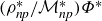 $({\rho _{\textit{np}}^*}/{\mathcal{M}_{\textit{np}}^*})\varPhi ^*$
. with
$({\rho _{\textit{np}}^*}/{\mathcal{M}_{\textit{np}}^*})\varPhi ^*$
. with $\varPhi ^\ast$
being the average volume concentration of particles, is conserved, therefore,
$\varPhi ^\ast$
being the average volume concentration of particles, is conserved, therefore,
 \begin{equation} \begin{aligned} \left (\frac {\rho _{\textit{np}}^*}{\mathcal{M}_{\textit{np}}^*}\right )I(\mathcal{D}^*)h_0^* \varPhi ^* &= \left [\int _{0}^{h_0^*}\left (\iint _{\mathcal{D}^*}\frac {\rho _{\textit{np}}^*}{\mathcal{M}_{\textit{np}}^*}\phi ^*\big(x^*,\,y^*,\,z^*,t^*\big)\text{d}x^*\text{d}y^*\right )\text{d}z^* \right. \nonumber \\ &\quad \left. +\, \iint _{{\mathscr{L}}^*}\varGamma ^*\big(x^*,\,y^*,\,t^*\big)\text{d}\textsf{S}^* \right ], \end{aligned} \end{equation}
with
 \begin{equation} \text{d}\textsf{S}^* = \sqrt {1+h_{x^*}^{*2}+h_{y^*}^{*2}}\,\text{d}x^*\text{d}y^*, \end{equation}
where $\mathcal{D}^*$
is a projection of the flow domain onto the
$\mathcal{D}^*$
is a projection of the flow domain onto the $x^\ast -y^\ast$
plane and
$x^\ast -y^\ast$
plane and $I({\mathcal{D}^*})$
is the area of this projection, whereas
$I({\mathcal{D}^*})$
is the area of this projection, whereas ${\mathscr{L}}^*$
represents the projection of the gas–liquid interface onto the
${\mathscr{L}}^*$
represents the projection of the gas–liquid interface onto the $x^*-y^*$
surface. Note that the average particle concentration
$x^*-y^*$
surface. Note that the average particle concentration $\varPhi ^*$
is multiplied by the volume, i.e.
$\varPhi ^*$
is multiplied by the volume, i.e. $I(\mathcal{D}^*)h_0^*$
, which expresses the total mass of nanoparticles across the volume of a nanofluid layer (Edmonstone et al. Reference Edmonstone, Craster and Matar2006). This implies that the total mass of nanoparticles in the bulk and at the interface is conserved; it also suggests an inherent inhomogeneity of nanoparticle distribution in the bulk and at the interface. A needed closure of the problem is obtained by imposing a constraint (2.28a
) with a prescribed and fixed value of
$I(\mathcal{D}^*)h_0^*$
, which expresses the total mass of nanoparticles across the volume of a nanofluid layer (Edmonstone et al. Reference Edmonstone, Craster and Matar2006). This implies that the total mass of nanoparticles in the bulk and at the interface is conserved; it also suggests an inherent inhomogeneity of nanoparticle distribution in the bulk and at the interface. A needed closure of the problem is obtained by imposing a constraint (2.28a
) with a prescribed and fixed value of $\varPhi ^*$
. We note that the condition of the constant nanoparticle averaged bulk concentration
$\varPhi ^*$
. We note that the condition of the constant nanoparticle averaged bulk concentration $\varPhi ^*$
is appropriate for the case of the quiescent base state. However, in the presence of the base state flow, the conservation of the nanoparticle mass flux or the nanoparticle concentration current should be employed (Krishnan, Beimfohr & Leighton Reference Krishnan, Beimfohr and Leighton1996; Frank et al. Reference Frank, Anderson, Weeks and Morris2003; Ramachandran & Leighton Reference Ramachandran and Leighton2008; Morris Reference Morris2020).
$\varPhi ^*$
is appropriate for the case of the quiescent base state. However, in the presence of the base state flow, the conservation of the nanoparticle mass flux or the nanoparticle concentration current should be employed (Krishnan, Beimfohr & Leighton Reference Krishnan, Beimfohr and Leighton1996; Frank et al. Reference Frank, Anderson, Weeks and Morris2003; Ramachandran & Leighton Reference Ramachandran and Leighton2008; Morris Reference Morris2020).
2.3. Dimensionless formulation
We non-dimensionalise the governing equation and the boundary conditions with the following normalisation:
 \begin{align} \big (x^*,y^*,z^* \big )=h_0^\ast \left (x,y,z\right ), \quad h^\ast =h_0^\ast h,\quad {\boldsymbol{u}^*}=\frac {\kappa ^\ast _{\textit{bf}}}{h_0^\ast } {\boldsymbol{u}}, \quad t^*=\frac {h_0^{*2}}{\nu ^\ast _{\textit{bf}}} t,\quad \phi ^* = \phi _m \phi , \nonumber \\ p^*=p^\ast _\infty +\frac {\mu ^\ast _{\textit{bf}}\kappa ^\ast _{\textit{bf}}}{h_0^{*2}} p, \quad T^*=T^\ast _\infty +\frac {q^\ast h_0^\ast }{K^\ast _{\textit{bf}}}T,\quad \varGamma ^* = \varGamma _\infty ^* \varGamma , \quad \varPhi ^*=\phi _m\varPhi , \nonumber \\ K^\ast _{\textit{nf}}=K^\ast _{\textit{bf}}K_{\textit{nf}},\quad \rho _{\textit{nf}}^* = \rho ^\ast _{\textit{bf}}\rho _{\textit{nf}}, \quad \mu _{\textit{nf}}^*=\mu ^\ast _{\textit{bf}} \mu _{\textit{nf}},\quad \big(\rho ^\ast c^\ast \big)_{\textit{nf}} =\big(\rho ^\ast c^\ast \big) _{\textit{bf}} (\rho c)_{\textit{nf}}.\quad \end{align}
From here and on, the quantities without an asterisk represent the variables in dimensionless form. A set of dimensionless governing equations is written as
 \begin{align} P(\rho _{\textit{nf}})_t+\boldsymbol{\nabla }\boldsymbol{\cdot }(\rho _{\textit{nf}}\boldsymbol{u}) &= 0, \end{align}
 \begin{align} (\rho _{\textit{nf}}\boldsymbol{u})_t + P^{-1}\boldsymbol{\nabla }\boldsymbol{\cdot }(\rho _{\textit{nf}}\boldsymbol{u}\boldsymbol{u}) &= -\boldsymbol{\nabla }p +\boldsymbol{\nabla }\boldsymbol{\cdot }\boldsymbol{\tau } - \rho _{\textit{nf}} G \boldsymbol{e}_z, \end{align}
 \begin{align} (\rho c)_{\textit{nf}}\left [PT_t + (\boldsymbol{u}\boldsymbol{\cdot }\boldsymbol{\nabla })T\right ] &= \boldsymbol{\nabla }\boldsymbol{\cdot }( K_{\textit{nf}}\boldsymbol{\nabla }T) , \end{align}
 \begin{align} PL^{-1}\phi _t + L^{-1}\boldsymbol{\nabla }\boldsymbol{\cdot }(\boldsymbol{u}\phi ) &= \boldsymbol{\nabla} ^2\phi + \boldsymbol{\nabla }\boldsymbol{\cdot }(\eta \phi \boldsymbol{\nabla }T), \end{align}
where $\displaystyle \boldsymbol{\nabla }\equiv ({\partial }/{\partial x}, {\partial }/{\partial y},{\partial }/{\partial z} )$
and
$\displaystyle \boldsymbol{\nabla }\equiv ({\partial }/{\partial x}, {\partial }/{\partial y},{\partial }/{\partial z} )$
and $\displaystyle \boldsymbol{\tau } =\mu _{\textit{nf}} [\boldsymbol{\nabla }{\boldsymbol u}+ \boldsymbol{\nabla }{\boldsymbol u}^\intercal -{2}/{3} (\boldsymbol{\nabla }\boldsymbol{\cdot }\boldsymbol{u} ) \boldsymbol{I} ]$
is the viscous part of the dimensionless stress tensor.
$\displaystyle \boldsymbol{\tau } =\mu _{\textit{nf}} [\boldsymbol{\nabla }{\boldsymbol u}+ \boldsymbol{\nabla }{\boldsymbol u}^\intercal -{2}/{3} (\boldsymbol{\nabla }\boldsymbol{\cdot }\boldsymbol{u} ) \boldsymbol{I} ]$
is the viscous part of the dimensionless stress tensor.
The non-dimensional form of the boundary conditions at the substrate $z=0$
reads
$z=0$
reads
 \begin{equation} \boldsymbol{u} = 0,\quad K_{\textit{nf}} T_z = 1, \quad \phi _z + \eta \phi T_z =0. \end{equation}
At the deformable interface $z=h(x,y,t)$
, the boundary conditions are
$z=h(x,y,t)$
, the boundary conditions are
 \begin{align} Ph_t+uh_x &+vh_y=w, \end{align}
 \begin{align} \boldsymbol{n} \boldsymbol{\cdot }\boldsymbol{\mathcal{T}}\boldsymbol{\cdot }\boldsymbol{n} = 2\boldsymbol{\mathcal{H}}\sigma ,\quad \boldsymbol{n} \boldsymbol{\cdot }\boldsymbol{\mathcal{T}}\boldsymbol{\cdot }\boldsymbol{x} &= \boldsymbol{x}\boldsymbol{\cdot }\boldsymbol{\nabla} _s \sigma ,\quad \boldsymbol{n}\boldsymbol{\cdot }\boldsymbol{\mathcal{T}}\boldsymbol{\cdot }\boldsymbol{y} = \boldsymbol{y}\boldsymbol{\cdot }\boldsymbol{\nabla} _s \sigma , \end{align}
where the dimensionless total stress tensor is $\boldsymbol{\mathcal{T}} = - p\boldsymbol{I} + \boldsymbol{\tau }$
and the normal and tangential vectors to the interface are
$\boldsymbol{\mathcal{T}} = - p\boldsymbol{I} + \boldsymbol{\tau }$
and the normal and tangential vectors to the interface are
 \begin{equation} \boldsymbol{n} = \frac {-h_{x}\boldsymbol{e}_{x}-h_{y}\boldsymbol{e}_{y}+\boldsymbol{e}_{z}}{\sqrt {1+h_{x}^{2}+h_{y}^{2}}},\quad \boldsymbol{x} = \frac {\boldsymbol{e}_{x}+h_{x}\boldsymbol{e}_z}{\sqrt {1+h_{x}^{2}}},\quad \boldsymbol{y} =\frac {\boldsymbol{e}_{y}+h_{y}\boldsymbol{e}_z}{\sqrt {1+h_{y}^{2}}},\quad \text{with}\quad 2\mathcal{H} = -\boldsymbol{\nabla} _s\boldsymbol{\cdot }\boldsymbol{n}, \end{equation}
and the surface tension is given by
 \begin{equation} \sigma = \varSigma _0 - M_T T + E \left [\omega _{\textit{np}} \left [\left (K_{\varSigma }-\phi \phi _m \right ) \ln \left (1-\varGamma \right )+K_{\varSigma } \varGamma \right ]-K_{\varSigma } \varGamma + \phi \phi _m \ln \left (\varGamma \right )\right ]. \end{equation}
The boundary conditions for heat and mass transfer at the deformable interface $z=h(x,y,t)$
are
$z=h(x,y,t)$
are
 \begin{align} K_{\textit{nf}}\boldsymbol{\nabla }T\boldsymbol{\cdot }\boldsymbol{n} & +BT=0, \end{align}
 \begin{align} P\big [\varGamma _{t}- h_{t}(\boldsymbol{e}_z\boldsymbol{\cdot }\boldsymbol{\nabla} _s )\varGamma \big ]+\boldsymbol{\nabla} _s\boldsymbol{\cdot }(\boldsymbol{u}_s\varGamma ) &+\varGamma (\boldsymbol{\nabla} _s\boldsymbol{\cdot }\boldsymbol{n})(\boldsymbol{u}\boldsymbol{\cdot }\boldsymbol{n}) = L_S\big (\boldsymbol{\nabla} _s^{2}\varGamma \big ) \nonumber\\ & + \mathcal{B}_A \big[K_{\textit{ad}}\phi (1-\varGamma ) - \varGamma \big ] , \end{align}
 \begin{align} -\left (\boldsymbol{\nabla }\phi + \eta \phi \boldsymbol{\nabla }T\right )\boldsymbol{\cdot }\boldsymbol{n} &= \mathcal{B}_D\left [K_{\textit{ad}}\phi (1-\varGamma ) - \varGamma \right ]. \end{align}
The problem possesses a long list of parameters, and the dynamics of the system is described by the following dimensionless numbers:
 \begin{equation} \begin{aligned} & P=\frac {\nu ^\ast _{\textit{bf}} \rho ^\ast _{\textit{bf}} c_{\textit{bf}}^\ast }{K^\ast _{\textit{bf}}}, \quad G=\frac {g^\ast h_0^{*3}}{\nu ^\ast _{\textit{bf}}\kappa ^\ast _{\textit{bf}}}, \quad L=\frac {C_B T^\ast _\infty \rho ^\ast _{\textit{bf}} c_{\textit{bf}}^\ast }{K^\ast _{\textit{bf}}}, \quad L_s=\frac {D_s \rho ^\ast _{\textit{bf}} c_{\textit{bf}}^\ast }{K^\ast _{\textit{bf}}}, \nonumber \\ & B=\frac {\widehat {q}h_0^\ast }{K^\ast _{\textit{bf}}},\qquad \varSigma _0 = \frac {\sigma ^\ast _rh_0^\ast }{\mu ^\ast _{\textit{bf}}\kappa ^\ast _{\textit{bf}}},\qquad \eta = \frac {C_T q^\ast h_0^\ast }{C_BT_\infty ^{\ast 2} K^\ast _{\textit{bf}}}. \end{aligned} \end{equation}
Here, $P,$
$P,$ $G,$
$G,$ $L,$
$L,$ $L_s,$ $B,$
$B,$ $\varSigma _0$
and
$\varSigma _0$
and $\eta ,$
are the Prandtl, modified Galileo, Lewis, surface Lewis, Biot, dimensionless surface tension numbers and the Soret coefficient, respectively. The convective heat transfer induces the interfacial surface tension gradient, which is quantified by the dimensionless thermal Marangoni number
$\eta ,$
are the Prandtl, modified Galileo, Lewis, surface Lewis, Biot, dimensionless surface tension numbers and the Soret coefficient, respectively. The convective heat transfer induces the interfacial surface tension gradient, which is quantified by the dimensionless thermal Marangoni number
 \begin{equation} M_T = \frac {\sigma _{T^*}^*\Delta T^{*}h_0^*}{\mu _{\textit{bf}}^*\kappa _{\textit{bf}}^*}, \quad \text{where}\quad \Delta T^*\equiv \frac {q^\ast h_0^\ast }{K^\ast _{\textit{bf}}}. \end{equation}
The interfacial adsorption and desorption processes are controlled by
 \begin{equation} K_{\textit{ad}} = \frac {k_a^* \rho _{\textit{np}}^*\phi _m\mathcal{S}_a^*}{\mathcal{M}_{\textit{np}}^*k_d^*},\quad \mathcal{B}_D = \frac {k_d^*h_0^*\mathcal{M}_{\textit{np}}^{*}}{C_BT_\infty ^*\phi _m\mathcal{S}_a^*\rho _{\textit{np}}^*},\quad \mathcal{B}_A = \frac {k_d^*h_0^{*2}}{\kappa _{\textit{bf}}^*}, \end{equation}
depicting the ratio of the adsorption to desorption rate, the surface diffusion and advection Biot numbers, respectively. The parameters $\mathcal{B}_D$
and
$\mathcal{B}_D$
and $\mathcal{B}_A$
denote the ratio of the desorption flux to the diffusion flux and to the advection flux, respectively. We finally note that the ratio between the two surface Biot numbers yields the dimensionless Péclet number
$\mathcal{B}_A$
denote the ratio of the desorption flux to the diffusion flux and to the advection flux, respectively. We finally note that the ratio between the two surface Biot numbers yields the dimensionless Péclet number $ Pe=\mathcal{B}_D/\mathcal{B}_A$
.
$ Pe=\mathcal{B}_D/\mathcal{B}_A$
.
In what follows, we define the dimensionless quantity, the Elasticity number
 \begin{equation} E = \frac {h_0^*K_B^*N_A^*T_\infty ^*\varGamma _b^*}{\mu _{\textit{bf}}^*\kappa _{\textit{bf}}^*}, \end{equation}
which describes the ratio of interfacial elasticity moduli at a fixed $\varGamma _b^*$
to viscous stress (Stebe et al. Reference Stebe, Lin and Maldarelli1991; Seiwert, Dollet & Cantat Reference Seiwert, Dollet and Cantat2014; Manikantan & Squires Reference Manikantan and Squires2020). Keeping in mind (2.25) for the surface tension implies that the Elasticity number intrinsically quantifies the variation of surface tension with interfacial nanoparticle concentration
$\varGamma _b^*$
to viscous stress (Stebe et al. Reference Stebe, Lin and Maldarelli1991; Seiwert, Dollet & Cantat Reference Seiwert, Dollet and Cantat2014; Manikantan & Squires Reference Manikantan and Squires2020). Keeping in mind (2.25) for the surface tension implies that the Elasticity number intrinsically quantifies the variation of surface tension with interfacial nanoparticle concentration $ \partial \sigma /\partial \varGamma$
and with bulk nanoparticle concentration
$ \partial \sigma /\partial \varGamma$
and with bulk nanoparticle concentration $\partial \sigma /\partial \phi$
. In fact, there exist two dynamic solutal Marangoni ‘numbers’ (more precisely, Marangoni functions), namely, the surface concentration Marangoni number
$\partial \sigma /\partial \phi$
. In fact, there exist two dynamic solutal Marangoni ‘numbers’ (more precisely, Marangoni functions), namely, the surface concentration Marangoni number
 \begin{equation} M_\varGamma (\varGamma ,\phi ) \equiv \frac {\partial \sigma }{\partial \varGamma } = \frac { E (1 -\varGamma +\varGamma \omega _{\textit{np}} ) (\varGamma K_{\varSigma }-\phi \phi _m )}{(\varGamma -1) \varGamma } \end{equation}
and the bulk concentration Marangoni number
 \begin{equation} M_\phi (\varGamma ) \equiv \frac {\partial \sigma }{\partial \phi } = E \phi _m \left [\ln (\varGamma )-\omega _{\textit{np}}\ln (1-\varGamma ) \right ]. \end{equation}
It is interesting to note that the surface concentration Marangoni number (2.34a ) exhibits dependence on both the interfacial nanoparticle concentration and the bulk nanoparticle concentration; however, the bulk concentration Marangoni number (2.34b ) depends only on the interfacial nanoparticle concentration. Remarkably, this signifies that the sign and amplitude of the surface tension gradient determine the mode of solutal Marangoni instability.
Variation of solutal Marangoni numbers $M_\phi$
and
$M_\phi$
and $M_\varGamma$
with nanoparticle concentration
$M_\varGamma$
with nanoparticle concentration $\phi$
obtained from (2.31e
) at equilibrium determined by (2.27) at
$\phi$
obtained from (2.31e
) at equilibrium determined by (2.27) at $E\approx 2.53,$ $K_{\textit{ad}} = 3.84,$ $K_\varSigma =2.11\times 10^{-3}$
and
$K_\varSigma =2.11\times 10^{-3}$
and $\omega _{\textit{np}}=6.23\times 10^3$
. The solid and dashed curves represent the variation of the surface concentration Marangoni number
$\omega _{\textit{np}}=6.23\times 10^3$
. The solid and dashed curves represent the variation of the surface concentration Marangoni number $M_\varGamma$
and the bulk concentration Marangoni number
$M_\varGamma$
and the bulk concentration Marangoni number $M_\phi$
, respectively.
$M_\phi$
, respectively.

Figure 3 displays the variations of the surface tension surface and bulk concentration gradients with the nanoparticle concentration obtained from (2.31e ) at an equilibrium interfacial nanoparticle concentration
 \begin{equation} \varGamma = \phi K_{\textit{ad}}/\left (1+\phi K_{\textit{ad}}\right ), \end{equation}
following from (2.27). We observe that $M_\varGamma$
increases linearly with the bulk nanoparticle concentration
$M_\varGamma$
increases linearly with the bulk nanoparticle concentration $\phi$
. The positivity of
$\phi$
. The positivity of $M_\varGamma$
for all values of the nanoparticle concentration suggests that the system inhibits a possible intrinsic solutocapillary instability due to the surface tension gradient of interfacial nanoparticle concentration
$M_\varGamma$
for all values of the nanoparticle concentration suggests that the system inhibits a possible intrinsic solutocapillary instability due to the surface tension gradient of interfacial nanoparticle concentration $M_\varGamma$
. However, we note that
$M_\varGamma$
. However, we note that $M_\phi$
is negative for low values of the bulk concentration
$M_\phi$
is negative for low values of the bulk concentration $\phi$
and positive otherwise.
$\phi$
and positive otherwise.
We further emphasise that the variation of surface tension due to the solutal effects is given by
 \begin{equation} \Delta \sigma = M_\varGamma \Delta \varGamma + M_\phi \Delta \phi = M_\varGamma \left ( \Delta \varGamma + \frac {M_\phi }{M_\varGamma } \Delta \phi \right ). \end{equation}
Note that, since $\Delta \varGamma$
and
$\Delta \varGamma$
and $\Delta \phi$
may be independently of either sign, it is impossible to claim whether
$\Delta \phi$
may be independently of either sign, it is impossible to claim whether $\Delta \sigma$
given by (2.36) leads to the emergence of the solutocapillary instability before obtaining the solution of the relevant EVP; see § 3.
$\Delta \sigma$
given by (2.36) leads to the emergence of the solutocapillary instability before obtaining the solution of the relevant EVP; see § 3.
It follows from figure 3 that there exists an intersection point $\tilde {M}$
corresponding to
$\tilde {M}$
corresponding to $\phi = \tilde {\phi }$
, so that
$\phi = \tilde {\phi }$
, so that $M_{\varGamma } \gt M_{\phi }$
for
$M_{\varGamma } \gt M_{\phi }$
for $\phi \lt \tilde {\phi }$
and
$\phi \lt \tilde {\phi }$
and $M_{\varGamma } \lt M_{\phi }$
for
$M_{\varGamma } \lt M_{\phi }$
for $\phi \gt \tilde {\phi }$
. The Elasticity number
$\phi \gt \tilde {\phi }$
. The Elasticity number $E$
reflects the impact of the variation of the surface tension with the bulk and interfacial concentration of particles under non-equilibrium conditions, and its value as an eigenvalue of the EVP referred to above is associated with the possible onset of the solutocapillary instability.
$E$
reflects the impact of the variation of the surface tension with the bulk and interfacial concentration of particles under non-equilibrium conditions, and its value as an eigenvalue of the EVP referred to above is associated with the possible onset of the solutocapillary instability.
The adsorption/desorption rates in the case of alumina nanoparticles in water can be derived using the interaction between a nanoparticle and the layer interface, as outlined by Ruckenstein & Prieve (Reference Ruckenstein and Prieve1976), Grow & Shaeiwitz (Reference Grow and Shaeiwitz1982) and Machrafi (Reference Machrafi2022) and detailed in Appendix A. We find the adsorption and desorption rates for Al $_2$
O
$_2$
O $_3$
nanoparticles of diameter
$_3$
nanoparticles of diameter $d_p^*=50$
nm to be
$d_p^*=50$
nm to be $k_a^* = 2.27\times 10^{-4}$
ms−1 and
$k_a^* = 2.27\times 10^{-4}$
ms−1 and $k_d^* = 2.3\times 10^3$
s
$k_d^* = 2.3\times 10^3$
s $^{-1}$
, respectively. Thereby, we obtain the values of the surface Biot numbers for a thin nanofluid layer
$^{-1}$
, respectively. Thereby, we obtain the values of the surface Biot numbers for a thin nanofluid layer $h_0^*=10^{-6}$
m as
$h_0^*=10^{-6}$
m as $\mathcal{B}_D = 6.7236$
and
$\mathcal{B}_D = 6.7236$
and $\mathcal{B}_A = 0.0157$
. The representative Péclet number obtained by the ratio of the surface Biot number yields
$\mathcal{B}_A = 0.0157$
. The representative Péclet number obtained by the ratio of the surface Biot number yields $ Pe \approx 426$
, which implies that the advective flux dominates the diffusive flux; hence, we refer to this case as a high-Péclet-number flow
$ Pe \approx 426$
, which implies that the advective flux dominates the diffusive flux; hence, we refer to this case as a high-Péclet-number flow $ Pe \gg 1$
. Moreover, for a thicker layer
$ Pe \gg 1$
. Moreover, for a thicker layer $h_0\approx 10^{-4}$
m or for a layer with a higher desorption rate
$h_0\approx 10^{-4}$
m or for a layer with a higher desorption rate $(k_d^* \approx 10^5)$
, the Péclet number reduces significantly to the case of
$(k_d^* \approx 10^5)$
, the Péclet number reduces significantly to the case of $ Pe \sim O(1)$
. Besides, there also exists a regime of
$ Pe \sim O(1)$
. Besides, there also exists a regime of $ Pe \ll 1$
, where the diffusion is faster than the advection (Manikantan & Squires Reference Manikantan and Squires2020). The other parameter ranges for the investigation of the current paper are provided in table 1.
$ Pe \ll 1$
, where the diffusion is faster than the advection (Manikantan & Squires Reference Manikantan and Squires2020). The other parameter ranges for the investigation of the current paper are provided in table 1.
Parameter nomenclature and their typical values used in this investigation.

The dimensionless thermophysical properties appearing in the set of non-dimensional governing equations and boundary conditions (2.30) and (2.31) are defined as
 \begin{equation} \begin{aligned} \rho _{\textit{nf}}(\phi ) =(1-\phi \phi _m)+\phi \phi _m\rho _{\textit{np}},\quad (\rho c)_{\textit{nf}}(\phi ) = (1-\phi \phi _m)+ \phi \phi _m(\rho c)_{\textit{np}},\\ K_{\textit{nf}}(\phi ) = 1 + a \phi \phi _m,\quad \mu _{\textit{nf}}(\phi ) = (1-\phi )^{-2}. \end{aligned} \end{equation}
We finally express the dimensionless form of the conservation of the total particle volume across the nanofluid layer. Hence, following (2.28), the dimensionless conservation of the total nanoparticle volume across the layer is given by
 \begin{equation} I(\mathcal{D})\varPhi = \int _{0}^{1}\left (\iint _{\mathcal{D}}\phi (x,\,y,\,z,\,t)\text{d}x\,\text{d}y\right )\text{d}z + \mathcal{A} \iint _{{\mathscr{L}}}\varGamma (x,\,y,\,t)\, \text{d}\textsf{S} , \end{equation}
with
 \begin{equation} \text{d}\textsf{S} = \sqrt {1+h_{x}^{2}+h_{y}^{2}}\,\text{d}x\,\text{d}y, \end{equation}
where ${\mathcal{A} = ({\mathcal{M}_{\textit{np}}^*\varGamma _\infty ^*}/{\rho _{\textit{np}}^*h_0^*\phi _m}})$
represents the degree of particle adsorption factor at the liquid–gas interface.
${\mathcal{A} = ({\mathcal{M}_{\textit{np}}^*\varGamma _\infty ^*}/{\rho _{\textit{np}}^*h_0^*\phi _m}})$
represents the degree of particle adsorption factor at the liquid–gas interface.
2.4. Base state solution
We now obtain the quiescent $(\boldsymbol{u}=\boldsymbol{u}_0 = 0)$
steady state of the system with the flat interface
$(\boldsymbol{u}=\boldsymbol{u}_0 = 0)$
steady state of the system with the flat interface $z=1$
in terms of the components of temperature
$z=1$
in terms of the components of temperature $T_0(z)$
, bulk nanoparticle concentration
$T_0(z)$
, bulk nanoparticle concentration $\phi _0(z)$
, pressure
$\phi _0(z)$
, pressure $p_0(z)$
and interfacial particle concentration
$p_0(z)$
and interfacial particle concentration $\varGamma _0$
, which depend only on the vertical coordinate
$\varGamma _0$
, which depend only on the vertical coordinate $z$
. We note that for the base state, the variables are strongly coupled via the concentration-dependent thermophysical properties; therefore, the appropriately reduced (2.30) and (2.31) need to be solved simultaneously, i.e.
$z$
. We note that for the base state, the variables are strongly coupled via the concentration-dependent thermophysical properties; therefore, the appropriately reduced (2.30) and (2.31) need to be solved simultaneously, i.e.
 \begin{align} p_{0,z}= - G -G \phi _m (\rho _{\textit{np}}-1) \phi _0, \end{align}
 \begin{align} \left [(1+a \phi _m \phi _0)T_{0,z}\right ]_z =0, \end{align}
 \begin{align} \left (\phi _{0,z} + \eta \phi _0 T_{0,z}\right )_z=0, \end{align}
with the following boundary conditions:
 \begin{align} \left (1+a\phi _m\phi _0\right )T_{0,z} = 1,\qquad \phi _{0,z} + \eta \phi _0 T_{0,z} =0\quad \text{at}\quad z=0, \end{align}
 \begin{align} p_0 =0, \qquad (1+a \phi _m \phi _0)T_{0,z} +B T_0=0, \qquad \phi _{0,z} + \eta \phi _0 T_{0,z}=0\quad \text{at}\quad z=1. \end{align}
At the equilibrium, the adsorption and desorption kinetic fluxes balance each other; therefore, it follows from (2.31h ) that
 \begin{equation} K_{\textit{ad}}\phi _0(1)(1-\varGamma _0)-\varGamma _0 = 0. \end{equation}
The base state of the system satisfying (2.39) with boundary conditions (2.40) reads
 \begin{align} T_0 &= \frac {1}{\eta B}\biggl [B \ln \left (\frac {1}{a\phi _m}\mathcal{W}\left (\gamma (\varPhi ) a\phi _m \exp {\left (\gamma (\varPhi ) a\phi _m - \eta \right )}\right )\right )\nonumber\\ & -B \ln \left (\frac {1}{a\phi _m}\mathcal{W}\left (\gamma (\varPhi ) a\phi _m \exp {\left (\gamma (\varPhi ) a\phi _m - \eta z\right )}\right )\right ) - \eta \biggr ], \end{align}
 \begin{align} \phi _0 &=\frac {\mathcal{W}\left (\gamma (\varPhi ) a\phi _m \exp {\left (\gamma (\varPhi ) a\phi _m - \eta z\right )}\right )}{a\phi _m}, \end{align}
 \begin{align} \varGamma _0 &= \frac {K_{\textit{ad}} \mathcal{W}\left (\gamma (\varPhi ) a\phi _m \exp \left (\gamma (\varPhi ) a\phi _m - \eta \right )\right )}{K_{\textit{ad}} \mathcal{W}\left (\gamma (\varPhi ) a\phi _m \exp \left (\gamma (\varPhi ) a\phi _m - \eta \right )\right ) + a\phi _m}, \end{align}
 \begin{align} p_0 &= G (1-z) - \frac {1}{2 \eta a}\biggl \{G (\rho _{\textit{np}}-1) \biggl [\mathcal{W}\left (\gamma (\varPhi ) a\phi _m \exp {\left (\gamma (\varPhi ) a\phi _m - \eta \right )}\right ) \nonumber \\ & -\mathcal{W}\left (\gamma (\varPhi ) a\phi _m \exp {\left (\gamma (\varPhi ) a\phi _m - \eta z\right )}\right )\biggr ]\times \biggl [\mathcal{W}\left (\gamma (\varPhi ) a\phi _m \exp {\left (\gamma (\varPhi ) a\phi _m - \eta \right )}\right ) \nonumber \\ & +\mathcal{W}\left (\gamma (\varPhi ) a\phi _m \exp {\left (\gamma (\varPhi ) a\phi _m - \eta z\right )}\right )+2\biggr ]\biggr \}, \end{align}
where $\gamma (\varPhi )$
is a constant of integration to be determined below and
$\gamma (\varPhi )$
is a constant of integration to be determined below and $\mathcal{W}(z)$
is the principal branch of the Lambert W function (Corless et al. Reference Corless, Gonnet, Hare, Jeffrey and Knuth1996; Vallis, Parker & Tobias Reference Vallis, Parker and Tobias2019; Gandhi et al. Reference Gandhi, Nepomnyashchy and Oron2025c
) given by
$\mathcal{W}(z)$
is the principal branch of the Lambert W function (Corless et al. Reference Corless, Gonnet, Hare, Jeffrey and Knuth1996; Vallis, Parker & Tobias Reference Vallis, Parker and Tobias2019; Gandhi et al. Reference Gandhi, Nepomnyashchy and Oron2025c
) given by
 \begin{equation} z={\mathcal{W}}(z) \exp {\mathcal{W}}(z). \end{equation}
Finally, following (2.38), the conservation of the total particle volume in the bulk and at the interface is imposed by specifying the constant value of the average concentration of the nanoparticles $\varPhi$
, i.e.
$\varPhi$
, i.e.
 \begin{equation} \varPhi = \int _{0}^{1}\phi _0(z)\text{d}z + \mathcal{A} \varGamma _0, \end{equation}
whereby, we deduce the value of $\gamma (\varPhi )$
by substituting (2.41b
) and (2.41c
) into (2.43). We note that the value of the constant
$\gamma (\varPhi )$
by substituting (2.41b
) and (2.41c
) into (2.43). We note that the value of the constant $\gamma (\varPhi )$
depends on the system parameters
$\gamma (\varPhi )$
depends on the system parameters $a$
,
$a$
, $\phi _m$
,
$\phi _m$
, $\eta ,$ $K_{\textit{ad}}$
,
$K_{\textit{ad}}$
, $\varPhi$
,
$\varPhi$
, $\mathcal{A}$
and
$\mathcal{A}$
and $\rho _{\textit{np}}^*/\mathcal{M}_{\textit{np}}^*$
.
$\rho _{\textit{np}}^*/\mathcal{M}_{\textit{np}}^*$
.
Variation of the quiescent base state in terms of (a) the bulk concentration $\phi _0$
, and (b) temperature components presented as
$\phi _0$
, and (b) temperature components presented as $T_0(z)-T(z=1)$
with the transverse coordinate
$T_0(z)-T(z=1)$
with the transverse coordinate $z$
, with
$z$
, with $B=0.01,$ $\eta = 1.66,$ $a=7.47,$ $\varPhi = 0.01$
and different values of the temperature difference
$\varPhi = 0.01$
and different values of the temperature difference $\Delta T^*$
. The inset in panel (a) represents the variation of the interfacial nanoparticle concentration
$\Delta T^*$
. The inset in panel (a) represents the variation of the interfacial nanoparticle concentration $\varGamma _0$
with the Soret effect
$\varGamma _0$
with the Soret effect $\eta$
.
$\eta$
.

Figure 4 illustrates the variation of the base state components in terms of the nanoparticle concentration in the bulk $\phi _0(z)$
in figure 4(a) and the temperature
$\phi _0(z)$
in figure 4(a) and the temperature $T_0(z)$
in figure 4(b) with the coordinate
$T_0(z)$
in figure 4(b) with the coordinate $z$
at different values of the temperature difference
$z$
at different values of the temperature difference $\Delta T^*$
in the layer.
$\Delta T^*$
in the layer.
We note that the Soret effect with a positive Soret coefficient drives the nanoparticle flux from the hot interface $z=h$
to the cold substrate
$z=h$
to the cold substrate $z=0$
, thus creating a stable density stratification profile. We find that particle concentration profiles of the base state exhibit a nonlinear variation with height
$z=0$
, thus creating a stable density stratification profile. We find that particle concentration profiles of the base state exhibit a nonlinear variation with height $z$
, whereas for low values of
$z$
, whereas for low values of $\Delta T^\ast$
, the temperature profiles of the base state in figure 4(b) display an almost linear variation with
$\Delta T^\ast$
, the temperature profiles of the base state in figure 4(b) display an almost linear variation with $z$
. The nonlinear variation of
$z$
. The nonlinear variation of $T_0(z)$
becomes visible for higher values of the temperature difference
$T_0(z)$
becomes visible for higher values of the temperature difference $\Delta T^*$
(not shown in figure 4
b). Also, in contrast to the concentration profiles
$\Delta T^*$
(not shown in figure 4
b). Also, in contrast to the concentration profiles $\phi _0(z)$
, the temperature
$\phi _0(z)$
, the temperature $T_0(z)$
remains almost independent of the temperature difference
$T_0(z)$
remains almost independent of the temperature difference $\Delta T^*$
. The negative values of the temperature difference
$\Delta T^*$
. The negative values of the temperature difference $T_0(z)-T_0(z=1)$
express the fact that the values of the temperature in the bulk are lower than
$T_0(z)-T_0(z=1)$
express the fact that the values of the temperature in the bulk are lower than $T_\infty ^*$
. Furthermore, we note that the interfacial adsorption/desorption kinetics expressed by
$T_\infty ^*$
. Furthermore, we note that the interfacial adsorption/desorption kinetics expressed by $K_{\textit{ad}}$
describes the relative nanoparticle adsorption to desorption ratio from/to the layer adjacent to the interface. The inset of figure 4(a) displays the variation of the interfacial concentration
$K_{\textit{ad}}$
describes the relative nanoparticle adsorption to desorption ratio from/to the layer adjacent to the interface. The inset of figure 4(a) displays the variation of the interfacial concentration $\varGamma _0$
component of the base state with the Soret coefficient
$\varGamma _0$
component of the base state with the Soret coefficient $\eta$
. We find that for the nanofluid layer cooled at the substrate, the Soret effect and the desorption kinetics complement each other; therefore, an increase in the Soret coefficient
$\eta$
. We find that for the nanofluid layer cooled at the substrate, the Soret effect and the desorption kinetics complement each other; therefore, an increase in the Soret coefficient $\eta$
via an increase in the temperature difference
$\eta$
via an increase in the temperature difference $\Delta T^*$
substantially reduces the interfacial concentration
$\Delta T^*$
substantially reduces the interfacial concentration $\varGamma _0$
.
$\varGamma _0$
.
We note that the mathematical framework presented in this paper formally addresses a moderately dense nanofluid, i.e. $\varPhi \leqslant 0.1$
and
$\varPhi \leqslant 0.1$
and $\phi _0(z) \le 0.1$
for all
$\phi _0(z) \le 0.1$
for all $0 \le z \le 1$
. As observed in figure 4(a), due to the presence of the Soret effect, the particle concentration near a cool bottom is the highest, so the value of
$0 \le z \le 1$
. As observed in figure 4(a), due to the presence of the Soret effect, the particle concentration near a cool bottom is the highest, so the value of $\phi _0(0)$
is higher than the average particle concentration
$\phi _0(0)$
is higher than the average particle concentration $\varPhi$
by more than three times for the set of parameters given. Therefore, to rule out the emergence of high nanoparticle concentrations near the bottom
$\varPhi$
by more than three times for the set of parameters given. Therefore, to rule out the emergence of high nanoparticle concentrations near the bottom $z=0$
, we have to set a specific limitation, hereafter referred to as limitation (i), for our theory to be valid. Another limitation, hereafter referred to as limitation (ii), should be set for the upper bound of the temperature drop
$z=0$
, we have to set a specific limitation, hereafter referred to as limitation (i), for our theory to be valid. Another limitation, hereafter referred to as limitation (ii), should be set for the upper bound of the temperature drop $\Delta T^*$
across the layer to exclude the temperature sensitivity of the thermophysical properties of the nanofluid. To first address limitation (ii), we assume that the temperature drop across the layer
$\Delta T^*$
across the layer to exclude the temperature sensitivity of the thermophysical properties of the nanofluid. To first address limitation (ii), we assume that the temperature drop across the layer $\Delta T^*$
should not exceed
$\Delta T^*$
should not exceed $10$
K, thus limiting the heat flux
$10$
K, thus limiting the heat flux $q^*$
from above accordingly. Now, with this upper bound at hand, we seek the conditions to satisfy limitation (i). We note that the upper bound for limitation (i) depends on the full set of parameters of the system. For example, for the fixed parameter set of
$q^*$
from above accordingly. Now, with this upper bound at hand, we seek the conditions to satisfy limitation (i). We note that the upper bound for limitation (i) depends on the full set of parameters of the system. For example, for the fixed parameter set of $a=7.47,\, \phi _m=0.65,\, K_{\textit{ad}} = 3.84,\, \mathcal{A} = 0.014$
,
$a=7.47,\, \phi _m=0.65,\, K_{\textit{ad}} = 3.84,\, \mathcal{A} = 0.014$
, $\rho _{\textit{np}}^*/\mathcal{M}_{\textit{np}}^* = 0.034$
along with
$\rho _{\textit{np}}^*/\mathcal{M}_{\textit{np}}^* = 0.034$
along with $d_p^* = 50$
nm and the average particle concentration
$d_p^* = 50$
nm and the average particle concentration $\varPhi =0.01$
considered here, the temperature drop across the nanofluid layer should be
$\varPhi =0.01$
considered here, the temperature drop across the nanofluid layer should be $\Delta T^*\leq 7$
K, which corresponds in this case to
$\Delta T^*\leq 7$
K, which corresponds in this case to $\phi _0(0)\leqslant 0.095$
. Similarly, in terms of
$\phi _0(0)\leqslant 0.095$
. Similarly, in terms of $\varPhi$
, the upper bound due to limitation (i) should increase with a decrease in
$\varPhi$
, the upper bound due to limitation (i) should increase with a decrease in $\Delta T^*$
. For instance, for the same set of parameters, as specified above, with the temperature drop of
$\Delta T^*$
. For instance, for the same set of parameters, as specified above, with the temperature drop of $\Delta T^*=1$
K, the average particle concentration is limited to
$\Delta T^*=1$
K, the average particle concentration is limited to $\varPhi \leqslant 0.05$
. Accordingly, an upper bound for
$\varPhi \leqslant 0.05$
. Accordingly, an upper bound for $\Delta T^*$
imposes an upper bound for the admissible thermal Marangoni number
$\Delta T^*$
imposes an upper bound for the admissible thermal Marangoni number $M_T$
. For example, for a nanofluid layer considered here with thickness
$M_T$
. For example, for a nanofluid layer considered here with thickness $h_0^*=10^{-6}$
m, the admissible values of the thermal Marangoni number must satisfy
$h_0^*=10^{-6}$
m, the admissible values of the thermal Marangoni number must satisfy $M_T\leq 3.3$
.
$M_T\leq 3.3$
.
3. Linear stability analysis
In this section we investigate the linear stability of the quiescent base state $\boldsymbol{u}_0=0$
given by (2.41) and the flat interface at
$\boldsymbol{u}_0=0$
given by (2.41) and the flat interface at $h_0 = 1$
. We perturb the system variables around the base state components in the form
$h_0 = 1$
. We perturb the system variables around the base state components in the form
 \begin{equation} {\boldsymbol u} = {\boldsymbol u}_0+\bar {{\boldsymbol u}}= \bar {\boldsymbol u}, \!\quad\! p=p_0+\bar {p}, \!\quad\! T=T_0+\bar {T}, \!\quad\! \phi =\phi _0+\bar {\phi }, \!\quad\! \varGamma = \varGamma _0 + \bar {\varGamma }, \!\quad\! h = h_0 + \bar {\zeta }, \end{equation}
where the overbar decoration of the system variables denotes the perturbations of the respective fields. The equations (2.30)–(2.31) are then linearised. We note that the thermophysical properties depend on the local particle concentration; therefore, they are also linearised around the base state concentration component $\phi _0$
:
$\phi _0$
:
 \begin{equation} \left . \begin{array}{ll} \rho _{\textit{nf}} = \textsf{R}_0 + \bar {\textsf{R}} = \left [\phi _m (\rho _{\textit{np}}-1) \phi _0 + 1 \right ]+ \left [\phi _m (\rho _{\textit{np}}-1) \bar {\phi }\right ],\\ (\rho c)_{\textit{nf}} = \textsf{H}_0 + \bar {\textsf{H}} = \left [\phi _m ((\rho c) _{\textit{np}}-1) \phi _0 + 1 \right ]+ \left [\phi _m ((\rho c) _{\textit{np}}-1) \bar {\phi }\right ],\\ K_{\textit{nf}} =\textsf{K}_0 + \bar {\textsf{K}} = (a\phi _m \phi _0 +1) + \bar {\phi } a\phi _m ,\\ \mu _{\textit{nf}} = \textsf{M}_0 + \bar {\textsf{M}} = \frac {1}{(\phi _0-1)^2} -\frac {2 \bar {\phi }}{(\phi _0-1)^3} . \end{array}\right \} \end{equation}
Here, we denote a succinct symbol $\textsf{X}\equiv (\textsf{R},\textsf{H},\textsf{K},\textsf{M} )$
representing the non-dimensional thermophysical properties,
$\textsf{X}\equiv (\textsf{R},\textsf{H},\textsf{K},\textsf{M} )$
representing the non-dimensional thermophysical properties, $\rho _{\textit{nf}},$ $ (\rho c )_{\textit{nf}},$ $K_{\textit{nf}}$
and
$K_{\textit{nf}}$
and $\mu _{\textit{nf}}$
, respectively. The first term
$\mu _{\textit{nf}}$
, respectively. The first term $\textsf{X}_0\equiv (\textsf{R}_0,\textsf{H}_0,\textsf{K}_0,\textsf{M}_0 )$
and the second term
$\textsf{X}_0\equiv (\textsf{R}_0,\textsf{H}_0,\textsf{K}_0,\textsf{M}_0 )$
and the second term $\bar {\textsf{X}}\equiv (\bar {\textsf{R}},\bar {\textsf{M}}, \bar {\textsf{K}}, \bar {\textsf{H}} )$
in (3.2) denote the thermophysical properties with a
$\bar {\textsf{X}}\equiv (\bar {\textsf{R}},\bar {\textsf{M}}, \bar {\textsf{K}}, \bar {\textsf{H}} )$
in (3.2) denote the thermophysical properties with a $z$
-dependent base state concentration and the disturbances, respectively.
$z$
-dependent base state concentration and the disturbances, respectively.
The linearised set of governing equations reads, in the vector form,
 \begin{align} P \frac {\partial \bar {\textsf{R}}}{\partial t} + \textsf{R}_0 \boldsymbol{\nabla }\boldsymbol{\cdot }\bar {\boldsymbol u} &+ \frac {\text{d}\textsf{R}_0}{\text{d}z} \bar {w} = 0, \end{align}
 \begin{align} \textsf{R}_0\frac {\partial \bar {\boldsymbol u}}{\partial t} - \textsf{M}_0 \boldsymbol{\nabla} ^2 \bar {\boldsymbol u} -\frac 13 \textsf{M}_0 \boldsymbol{\nabla }\left ( \boldsymbol{\nabla }\boldsymbol{\cdot }\bar {\boldsymbol u} \right ) + \boldsymbol{\nabla }\bar p &+G \bar {\textsf{R}} {\boldsymbol e}_z - \frac {\text{d}\textsf{M}_0}{\text{d}z} \boldsymbol{\varepsilon }=0, \end{align}
 \begin{align} \textsf{H}_0 \left (P \frac {\partial \bar {T}}{\partial t} + \frac{\text{d}T_0}{\text{d}z}\bar {w}\right ) -\textsf{K}_0 \boldsymbol{\nabla} ^2 \bar {T} -\bar {\textsf{K}}\frac {d^2 T_0}{d z^2} &- \frac{\text{d}T_0}{\text{d}z}\frac {\partial \bar {\textsf{K}}}{\partial z} - \frac {d \textsf{K}_0}{\text{d}z}\frac {\partial \bar {T}}{\partial z} = 0, \end{align}
 \begin{align} PL^{-1}\frac {\partial \bar {\phi }}{\partial t} + \phi _0 L^{-1} \boldsymbol{\nabla }\boldsymbol{\cdot }\bar {\boldsymbol u} +\frac {\text{d}\phi _0}{\text{d}z} \!\left (L^{-1}\bar {w}-\eta \frac {\partial \bar {T}}{\partial z}\!\right ) &- \eta \phi _0\boldsymbol{\nabla} ^2 \bar T -\eta \frac {\partial }{\partial z} \!\left (\frac{\text{d}T_0}{\text{d}z} \bar \phi \!\right ) - \boldsymbol{\nabla} ^2 \bar \phi =0, \end{align}
where
 \begin{align} \boldsymbol{\varepsilon } = \left ( \begin{array}{c} \bar {u}_z+\bar {w}_x \\[5pt] \bar {v}_z+\bar {w}_y\\[5pt] 2 \bar {w}_z -\dfrac 23 \boldsymbol{\nabla }\boldsymbol{\cdot }\bar {\boldsymbol u} \end{array} \right ) \end{align}
is a vector containing the two off-diagonal and one diagonal components of the strain rate tensor associated with the $z$
direction. We note that (3.3a
)–(3.3d
) represent linearised versions of the continuity, three-dimensional momentum conservation, energy and mass diffusion equations, respectively.
$z$
direction. We note that (3.3a
)–(3.3d
) represent linearised versions of the continuity, three-dimensional momentum conservation, energy and mass diffusion equations, respectively.
The linearised boundary conditions at the solid substrate $z=0$
are
$z=0$
are
 \begin{equation} \bar {\boldsymbol{u}}=0,\quad \textsf{K}_0\frac {\partial \bar {T}}{\partial z} + \bar {\textsf{K}}\frac{\text{d}T_0}{\text{d}z} = 0,\quad \eta \phi _0 \frac {\partial \bar {T}}{\partial z} + \eta \frac{\text{d}T_0}{\text{d}z} \bar {\phi } + \frac {\partial \bar {\phi }}{\partial z}=0. \end{equation}
The linearised form of the boundary conditions at the interface $z=1$
are
$z=1$
are
 \begin{align} &\qquad \qquad \qquad \qquad \qquad \qquad P\frac {\partial \bar {\zeta }}{\partial t} - \bar {w} =0, \end{align}
 \begin{align} &\frac {d p_0}{\text{d}z}\bar {\zeta } + \bar {p} + \frac {2}{3} \textsf{M}_0\left ( \boldsymbol{\nabla }\boldsymbol{\cdot }\bar {\boldsymbol u} - 3 \frac {\partial \bar {w}}{\partial z}\right ) + \boldsymbol{\nabla} _\perp ^2 \bar {\zeta } \Big \{\varSigma _0 - M_T T_0 \nonumber\\ &\quad +\, E \big [K_{\varSigma } \left (\omega _{\textit{np}}\left (\varGamma _0+ \ln (1-\varGamma _0)\right ) - \varGamma _0\right ) + \phi _0 \phi _m \left (\ln (\varGamma _0)-\omega _{\textit{np}}\ln (1-\varGamma _0) \right )\big ]\Big \} = 0, \end{align}
 \begin{align} & \textsf{M}_0 \boldsymbol{\varepsilon }_\perp + M_T \left (\boldsymbol{\nabla} _\perp \bar {T}+\frac{\text{d}T_0}{\text{d}z}\boldsymbol{\nabla} _\perp \bar {\zeta } \right ) + E\biggl [-\frac {K_{\varSigma } \left (\varGamma _0 (\omega _{\textit{np}} - 1)+1\right ) \boldsymbol{\nabla} _\perp \bar {\varGamma }}{\varGamma _0-1} \nonumber\\ &\quad + \phi _m\biggl (\frac {\phi _0 \left (\varGamma _0 (\omega _{\textit{np}} - 1)+1\right )\boldsymbol{\nabla} _\perp \bar {\varGamma }}{(\varGamma _0-1) \varGamma _0} \nonumber\\ &\quad - \left ( \ln (\varGamma _0) - \omega _{\textit{np}} \ln \left (1-\varGamma _0\right ) \right ) \left (\boldsymbol{\nabla} _\perp \bar {\phi }+\frac {\text{d}\phi _0}{\text{d}z}\boldsymbol{\nabla} _\perp \bar {\zeta } \right )\biggr )\biggr ] = 0, \end{align}
 \begin{align} &\bar {\textsf{K}}\frac{\text{d}T_0}{\text{d}z} + \textsf{K}_0\frac {\partial \bar {T}}{\partial z} + \left [\frac{\text{d}T_0}{\text{d}z} \left (B+ \frac {d \textsf{K}_0}{\text{d}z}\right )+ \textsf{K}_0 \frac {d^2T_0}{d z^2}\right ] \bar {\zeta } + B \bar {T} =0, \end{align}
 \begin{align} & \frac {\partial \bar {\phi }}{\partial z}+ \left [\eta \frac{\text{d}T_0}{\text{d}z} \frac {d \phi _0}{\text{d}z} + \eta \phi _0\frac {d^2 T_0}{d z^2} + \frac {d^2\phi _0}{d z^2}\right ] \bar {\zeta } + \eta \frac{\text{d}T_0}{\text{d}z} \bar {\phi } + \eta \phi _0 \frac {\partial \bar {T}}{\partial z} \nonumber\\ &\quad = \mathcal{B}_D\biggl [\bar {\varGamma }\left (\phi _0 K_{\textit{ad}}+1\right ) + K_{\textit{ad}}\left (\varGamma _0-1\right ) \left (\frac {\text{d}\phi _0}{\text{d}z}\bar {\zeta } + \bar {\phi }\right )\biggr ], \end{align}
 \begin{align} & P \frac {\partial \bar {\varGamma }}{\partial t} + \varGamma _0\boldsymbol{\nabla} _\perp \boldsymbol{\cdot }\bar {\boldsymbol{u}}_s -L_s\boldsymbol{\nabla} _\perp ^2\bar {\varGamma } + \mathcal{B}_A\biggl [\bar {\varGamma } \left (\phi _0 K_{\textit{ad}}+1\right ) +(\varGamma _0 - 1) K_{\textit{ad}} \left (\frac {\text{d}\phi _0}{\text{d}z} \bar {\zeta } + \bar {\phi }\right )\biggr ] = 0, \end{align}
where $\displaystyle \boldsymbol{\nabla} _\perp \equiv ({\partial }/{\partial x}, {\partial }/{\partial y} )^\intercal ,$ $\bar {\boldsymbol{u}}_s = (\bar {u},\bar {v},0 )$
and
$\bar {\boldsymbol{u}}_s = (\bar {u},\bar {v},0 )$
and
 \begin{align} \boldsymbol{\varepsilon }_\perp = \left ( \begin{array}{c} \bar {u}_z+\bar {w}_x \\ \bar {v}_z+\bar {w}_y \end{array} \right ). \end{align}
Note that it is possible to express the linearised continuity of tangential stress balance at the deformable interface (3.6c ) in terms of the dynamic solutal Marangoni numbers (functions), given by (2.34a ) and (2.34b ):
 \begin{align} \textsf{M}_0 \boldsymbol{\varepsilon }_\perp + M_T \!\left (\boldsymbol{\nabla} _\perp \bar {T}+\frac{\text{d}T_0}{\text{d}z}\boldsymbol{\nabla} _\perp \bar {\zeta } \!\right ) - M_{\phi }(\varGamma _0) \!\left [\boldsymbol{\nabla} _\perp \bar {\phi } + \frac {\textrm{d}\phi _0}{\textrm{d}z}\boldsymbol{\nabla} _\perp \bar {\zeta }\!\right ] - M_\varGamma (\varGamma _0,\phi _0)\boldsymbol{\nabla} _\perp \bar {\varGamma } = 0. \end{align}
We remind that in our case, the surface tension varies non-monotonically with nanoparticle concentration at the interface (figure 3); therefore, the signs of the thermal and solutal contributions in (3.8) are different.
Equations (3.6) represent the linearised versions of the kinematic boundary condition, the balance of normal stresses, the two-dimensional balance of tangential stresses, the heat transfer boundary condition, the balance of mass fluxes and the boundary condition governing the evolution of the interfacial concentration, respectively. Moreover, we mention that in (3.6b
) and (3.6c
), the perturbations of the interfacial concentration $\bar {\varGamma }$
are represented by the linearisation of the surface tension using the Taylor expansion around
$\bar {\varGamma }$
are represented by the linearisation of the surface tension using the Taylor expansion around $\varGamma _0$
.
$\varGamma _0$
.
We find that the given problem has the symmetry $x\leftrightarrow y$
and
$x\leftrightarrow y$
and $u\leftrightarrow v$
. Hence, we constrain our system to the two-dimensional case in the
$u\leftrightarrow v$
. Hence, we constrain our system to the two-dimensional case in the $x{-}z$
plane. We note that the thermophysical properties, such as density, viscosity and thermal conductivity, do not depend on pressure. Furthermore, we postulate our assumption by satisfying the condition
$x{-}z$
plane. We note that the thermophysical properties, such as density, viscosity and thermal conductivity, do not depend on pressure. Furthermore, we postulate our assumption by satisfying the condition $\displaystyle {\mathcal{U}^*/c^{*}\ll 1,}$
where
$\displaystyle {\mathcal{U}^*/c^{*}\ll 1,}$
where $\displaystyle {\mathcal{U}^*=\kappa ^*_{\textit{bf}}/h_0^*}$
is the characteristic velocity scale and
$\displaystyle {\mathcal{U}^*=\kappa ^*_{\textit{bf}}/h_0^*}$
is the characteristic velocity scale and $c^*$
is the speed of sound, for water as a base fluid
$c^*$
is the speed of sound, for water as a base fluid $c^* = 1470$
ms−1 (Batchelor Reference Batchelor2000). In what follows, we eliminate the pressure from the problem by applying the
$c^* = 1470$
ms−1 (Batchelor Reference Batchelor2000). In what follows, we eliminate the pressure from the problem by applying the $\boldsymbol{\nabla }\times$
operator to the momentum conservation equations and by differentiating the normal stress balance boundary condition along the interface, followed by substituting there the pressure gradient components obtained from the momentum conservation equations.
$\boldsymbol{\nabla }\times$
operator to the momentum conservation equations and by differentiating the normal stress balance boundary condition along the interface, followed by substituting there the pressure gradient components obtained from the momentum conservation equations.
We now introduce the normal perturbation modes to the system variables,
 \begin{equation} \big (\bar u, \bar {w}, \bar {T}, \bar {\phi }, \bar {\zeta }, \bar {\varGamma } ; \bar {\textsf{X}}\big ) (x,z,t) = \left (u(z), w(z),\theta (z),\varphi (z),\zeta ,\varGamma ; \textsf{X}\right )\exp (ikx+\lambda t), \end{equation}
where $u,\, w,\, \theta ,$ $\varphi ,$ $\zeta ,$ $\varGamma $
and
$\varGamma $
and $\textsf{X} \equiv (\textsf{R}(z),\textsf{M}(z), \textsf{K}(z), \textsf{H}(z) )$
are the amplitudes of the horizontal and vertical fluid velocity components, temperature, bulk nanoparticle concentration, interfacial deformation, interfacial nanoparticle concentration and material properties (all expressed via
$\textsf{X} \equiv (\textsf{R}(z),\textsf{M}(z), \textsf{K}(z), \textsf{H}(z) )$
are the amplitudes of the horizontal and vertical fluid velocity components, temperature, bulk nanoparticle concentration, interfacial deformation, interfacial nanoparticle concentration and material properties (all expressed via $\varphi$
) perturbations, respectively. We determine the stability of the system with respect to the disturbance wavenumber
$\varphi$
) perturbations, respectively. We determine the stability of the system with respect to the disturbance wavenumber $k\in \mathbb{R}$
via the growth rate
$k\in \mathbb{R}$
via the growth rate $\lambda \in \mathbb{C}$
of the disturbances. In this representation, the negative and positive values of the real part of the growth rate
$\lambda \in \mathbb{C}$
of the disturbances. In this representation, the negative and positive values of the real part of the growth rate $\lambda$
correspond to the stability and instability regimes of the system, respectively. We note that
$\lambda$
correspond to the stability and instability regimes of the system, respectively. We note that $\textsf{X}$
represents the material properties of the nanofluid, which are concentration dependent and do not introduce additional dependent variables following (3.2).
$\textsf{X}$
represents the material properties of the nanofluid, which are concentration dependent and do not introduce additional dependent variables following (3.2).
The following EVP is obtained from (3.6) and (3.9) to determine the growth rate $\lambda$
of the disturbance as a function of its wavenumber
$\lambda$
of the disturbance as a function of its wavenumber $k$
for a specified parameter set:
$k$
for a specified parameter set:
 \begin{align} \textsf{R}_0 \big (w^{\prime }+i k u\big ) &+\lambda P \textsf{R} + w \textsf{R}_0^{\prime }=0, \end{align}
 \begin{align} -i G k \textsf{R} + k^2 \textsf{M}_0 u^{\prime } + 2 k^2 u \textsf{M}_0^{\prime } &- i k w \big (k^2 \textsf{M}_0 + \lambda \textsf{R}_0 +\textsf{M}_0^{\prime \prime } \big )+i k \textsf{M}_0 w^{\prime \prime } \nonumber\\ -u^{\prime \prime \prime } \textsf{M}_0 &-2 u^{\prime \prime } \textsf{M}_0^{\prime } + \lambda \textsf{R}_0 u^{\prime } - u^{\prime } \textsf{M}_0^{\prime \prime }+\lambda u \textsf{R}_0^{\prime } = 0, \end{align}
 \begin{align} -T_0^{\prime \prime } \textsf{K} + \theta \big (k^2 \textsf{K}_{0} + \lambda P \textsf{H}_{0} \big ) &+T_0^{\prime } \big (w \textsf{H}_{0} - \textsf{K}^\prime \big )-\textsf{K}_{0} \theta ^{\prime \prime } - \textsf{K}_{0}^{\prime } \theta ^{\prime } = 0, \end{align}
 \begin{align} \varphi \big (k^2 L-\eta L T_0^{\prime \prime } + \lambda P\big )+\eta k^2 L \theta \phi _0 &+ \phi _0 \big (i k u - \eta L \theta ^{\prime \prime } + w^{\prime } \big ) \nonumber\\ &+\phi _0^{\prime } \big (w - \eta L \theta ^{\prime } \big ) -\eta L T_0^{\prime } \varphi ^{\prime } - L \varphi ^{\prime \prime } =0. \end{align}
The boundary conditions at the solid substrate $z=0$
are
$z=0$
are
 \begin{equation} \boldsymbol{u}=0,\quad \left (a \phi _m \phi _0+1\right ) \theta ^{\prime } + a\phi _m T_0^{\prime } \varphi =0,\quad \eta \phi _0 \theta ^{\prime } + \eta T_0^{\prime } \varphi + \varphi ^{\prime }=0. \end{equation}
At the interface $z=1$
, the boundary conditions following the projection from the deformable interface
$z=1$
, the boundary conditions following the projection from the deformable interface $z=h$
read
$z=h$
read
 \begin{align} &\qquad \qquad \qquad \qquad \qquad \qquad \qquad \zeta \lambda P-w =0, \end{align}
 \begin{align} & u \big (2 k^2 \textsf{M}_{0} + \lambda \textsf{R}_{0} \big )+i \left (-\zeta k p_0^{\prime } + k \textsf{M}_{0} w^{\prime } - k \textsf{M} _{0}^{\prime } w+i \textsf{M}_{0} u^{\prime \prime } + i \textsf{M}_{0}^{\prime } u^{\prime }\right )\nonumber\\ &\quad + i \zeta k^3 [ \varSigma _0 - M_T T_0 + E (K_{\varSigma } (\varGamma _0 (\omega _{\textit{np}}-1)+ \omega _{\textit{np}}\ln (1 - \varGamma _0) ) \nonumber\\ &\quad + \phi _0 \phi _m (\ln (\varGamma _0)- \omega _{\textit{np}} \ln (1-\varGamma _0) )) ] =0, \end{align}
 \begin{align} & \textsf{M}_{0} \big (k w-i u^{\prime }\big ) + k M_T \big (\zeta T_0^{\prime } + \theta \big ) - \frac {k E}{(\varGamma _0-1) \varGamma _0} \biggl [\varGamma \varGamma _0 K_{\varSigma } \left (\varGamma _0 (\omega _{\textit{np}}-1)+1\right ) \nonumber\\ &\quad + \phi _m \biggl (-\varGamma \phi _0 + \varGamma _0^2 \left (\ln \left (\varGamma _0\right )- \omega _{\textit{np}}\ln \left (1-\varGamma _0\right ) \right ) \left (\zeta \phi _0^\prime + \varphi \right ) \nonumber\\ &\quad + \varGamma _0 \biggl (-\zeta \ln \left (\varGamma _0\right ) \phi _0^\prime + \varGamma \phi _0 + \omega _{\textit{np}} \left (\zeta \ln \left (1-\varGamma _0\right ) \phi _0^\prime -\varGamma \phi _0 \right )\nonumber\\ &\quad + \varphi \left ( \omega _{\textit{np}}\ln \left (1-\varGamma _0\right ) - \ln \left (\varGamma _0\right )\right )\biggr )\biggr )\biggr ] =0, \end{align}
 \begin{align} & T_0^{\prime } \left [a\phi _m \left (\zeta \phi _0^{\prime } + \varphi \right )+B \zeta \right ]+\left ( a\phi _m \phi _0 +1\right ) \theta ^{\prime } + \zeta T_0^{\prime \prime } \left (a\phi _m \phi _0 +1\right )+B \theta =0, \end{align}
 \begin{align} & \zeta \phi _0^{\prime \prime } + \eta \phi _0 \big (\theta ^{\prime } + \zeta T_0^{\prime \prime }\big )+\eta T_0^{\prime } \big (\zeta \phi _0^{\prime } + \varphi \big )+\varphi ^{\prime } \nonumber \\ &\quad = \mathcal{B}_D \left [K_{\textit{ad}} \left (\left (\varGamma _0 - 1\right ) \zeta \phi _0^\prime + \varGamma \phi _0 + \left (\varGamma _0 - 1\right ) \varphi \right ) + \varGamma \right ] , \end{align}
 \begin{align} & P\lambda \varGamma + \varGamma k^2 L_s + i \varGamma _0 k u + \mathcal{B}_A \left [K_{\textit{ad}} \left (\left (\varGamma _0 - 1\right ) \zeta \phi _0^\prime + \varGamma \phi _0 + \left (\varGamma _0 - 1\right ) \varphi \right ) + \varGamma \right ] = 0 . \end{align}
We recall that $\textsf{R}_0,\textsf{M}_0, \textsf{K}_0, \textsf{H}_0$
represent the values of the thermophysical properties of the system given by (3.2), while
$\textsf{R}_0,\textsf{M}_0, \textsf{K}_0, \textsf{H}_0$
represent the values of the thermophysical properties of the system given by (3.2), while $\textsf{R},\textsf{M}, \textsf{K}, \textsf{H}$
are the amplitudes of their respective disturbances depending on
$\textsf{R},\textsf{M}, \textsf{K}, \textsf{H}$
are the amplitudes of their respective disturbances depending on $z$
. Additionally, we mention that the perturbations of the bulk and interfacial concentrations introduce an additional inhomogeneity in the bulk and at the interface, thereby leading to the inhomogeneity of the thermophysical properties. This implies that the nanoparticle concentration displays an inhomogeneous profile across the lateral plane, although the total volume of the nanoparticle concentration is conserved automatically due to the periodicity in
$z$
. Additionally, we mention that the perturbations of the bulk and interfacial concentrations introduce an additional inhomogeneity in the bulk and at the interface, thereby leading to the inhomogeneity of the thermophysical properties. This implies that the nanoparticle concentration displays an inhomogeneous profile across the lateral plane, although the total volume of the nanoparticle concentration is conserved automatically due to the periodicity in $x$
.
$x$
.
3.1. Numerical procedure and the incompressibility condition
We further simplify the EVP (3.10) by substituting the expression of the perturbed longitudinal velocity component $u$
from (3.10a
) into the rest of the equations of the EVP (3.10). We also extract the expression of the perturbed deformation
$u$
from (3.10a
) into the rest of the equations of the EVP (3.10). We also extract the expression of the perturbed deformation $\zeta$
from (3.10g
) and substitute it into the rest of the boundary conditions at
$\zeta$
from (3.10g
) and substitute it into the rest of the boundary conditions at $z=1$
. We note that the system consists of two concentration fields, the bulk concentration
$z=1$
. We note that the system consists of two concentration fields, the bulk concentration $\varphi$
and the interfacial concentration
$\varphi$
and the interfacial concentration $\varGamma$
, to accommodate the numerical implementation of the EVP, we combine the boundary condition for the bulk mass flux balance equation (3.10j
) with the evolution boundary condition for the interfacial concentration equation (3.10k
), and obtain an explicit expression of the disturbances of the interfacial concentration
$\varGamma$
, to accommodate the numerical implementation of the EVP, we combine the boundary condition for the bulk mass flux balance equation (3.10j
) with the evolution boundary condition for the interfacial concentration equation (3.10k
), and obtain an explicit expression of the disturbances of the interfacial concentration $\varGamma$
. In what follows, we substitute the obtained expression of
$\varGamma$
. In what follows, we substitute the obtained expression of $\varGamma$
into the rest of the boundary conditions at
$\varGamma$
into the rest of the boundary conditions at $z=1$
. Hence, our simplified EVP reduces to contain only three dependent perturbed variables
$z=1$
. Hence, our simplified EVP reduces to contain only three dependent perturbed variables $w,$
$w,$ $\theta $
and
$\theta $
and $\varphi$
.
$\varphi$
.
The solution of the linear EVP gives us the threshold values of the instabilities. We solve the EVP and its simplifications using open-source code (Pearce et al. Reference Pearce, Heil, Jensen, Jones and Prokop2018). It is based on the shooting method and the numerical construction of the complex-valued Evans function (Evans & Feroe Reference Evans and Feroe1977) using the compound matrix method (Ng & Reid Reference Ng and Reid1979) whose roots represent the eigenvalues of the given problem. The solution is initiated by specifying the range in which the roots of the Evans function are searched and adjusted if needed. More details related to the numerical implementation are provided in Gandhi et al. (Reference Gandhi, Nepomnyashchy and Oron2025c ); Appendix C presents a validation of the numerical method by comparing the results of the fully numerical solution of the EVP with the analytical solutions of the toy problem of § 4.3.
We note that the density of the nanofluid system varies with space and time and also depends on the local nanoparticle concentration, which in turn varies spatiotemporally. Hence, under this consideration, the system is ‘compressible’. As in Gandhi et al. (Reference Gandhi, Nepomnyashchy and Oron2025c ), a further simplification of the problem considered here can be achieved. We rewrite the non-dimensional form of the nanofluid continuity equation (2.30a ) as
 \begin{equation} \boldsymbol{\nabla }\boldsymbol{\cdot }\boldsymbol{u} = -\big (\rho _{\textit{np}}-1\big )\phi _m\left [P\phi _t + \boldsymbol{\nabla }\boldsymbol{\cdot }\left (\phi \boldsymbol{u}\right )\right ]. \end{equation}
Based on (3.11) and on the nanoparticle mass flux balance equation (2.30d ), the divergence of the velocity vector is obtained in the form
 \begin{equation} \boldsymbol{\nabla }\boldsymbol{\cdot }\boldsymbol{u} = -L\big (\rho _{\textit{np}}-1\big ) \phi _m\big [\boldsymbol{\nabla} ^2\phi + \boldsymbol{\nabla }\boldsymbol{\cdot } (\eta \phi \boldsymbol{\nabla }T )\big ]. \end{equation}
The right-hand side of (3.12) represents the deviation of the full ‘compressible’ system from an incompressible one. For nanosuspension with small concentration, e.g. $\varPhi \leqslant 0.05$
, and the small Lewis number
$\varPhi \leqslant 0.05$
, and the small Lewis number $L\in (10^{-5},10^{-3} )$
, the right-hand side of (3.12) effectively vanishes and yields
$L\in (10^{-5},10^{-3} )$
, the right-hand side of (3.12) effectively vanishes and yields $\boldsymbol{\nabla }\boldsymbol{\cdot }\boldsymbol{u}\approx 0$
. This implies that under these conditions, the system at hand can be treated as ‘incompressible’. In our previous studies Gandhi et al. (Reference Gandhi, Nepomnyashchy and Oron2025c
), we validated the underlying incompressibility assumption via a direct comparison between the solution of the full EVP in its compressible and incompressible forms. Henceforth, we solve the EVP (3.10) under the assumption of an incompressible fluid system.
$\boldsymbol{\nabla }\boldsymbol{\cdot }\boldsymbol{u}\approx 0$
. This implies that under these conditions, the system at hand can be treated as ‘incompressible’. In our previous studies Gandhi et al. (Reference Gandhi, Nepomnyashchy and Oron2025c
), we validated the underlying incompressibility assumption via a direct comparison between the solution of the full EVP in its compressible and incompressible forms. Henceforth, we solve the EVP (3.10) under the assumption of an incompressible fluid system.
4. Results and discussion
In a layer of a pure Newtonian liquid, cooling at the substrate greatly facilitates the Marangoni mechanism to stabilise the layer and also to suppress the gravity-driven Rayleigh–Taylor instability (Deissler & Oron Reference Deissler and Oron1992; Oron & Rosenau Reference Oron and Rosenau1992; Burgess et al. Reference Burgess, Juel, McCormick, Swift and Swinney2001; Alexeev & Oron Reference Alexeev and Oron2007). Nanofluids with a positive Soret coefficient in a gravity field display the formation of a stable stratification across the layer due to the emergence of the nanoparticle concentration profile decreasing with height $z$
, as shown in figure 4(a). On the other hand, cooling on the substrate induces solutocapillary instability in nanofluid layers with no kinetics taking place at the interface (Gandhi et al. Reference Gandhi, Nepomnyashchy and Oron2025c
). Additionally, we note that irrespective of the direction of heating, the spatial redistribution of nanoparticles due to adsorption/desorption kinetics causes concentration inhomogeneity, which leads to the onset of solutocapillary instability (Shmyrov et al. Reference Shmyrov, Mizev, Demin, Petukhov and Bratsun2019).
$z$
, as shown in figure 4(a). On the other hand, cooling on the substrate induces solutocapillary instability in nanofluid layers with no kinetics taking place at the interface (Gandhi et al. Reference Gandhi, Nepomnyashchy and Oron2025c
). Additionally, we note that irrespective of the direction of heating, the spatial redistribution of nanoparticles due to adsorption/desorption kinetics causes concentration inhomogeneity, which leads to the onset of solutocapillary instability (Shmyrov et al. Reference Shmyrov, Mizev, Demin, Petukhov and Bratsun2019).
Monotonic pure solutocapillary instability at $\varPhi = 0.01,$ $a=7.47,$ $\eta =1.66,$ $L=L_s = 6\times 10^{-5},$ $\mathcal{B}_A=0.01578,$ $\mathcal{B}_D=6.7236,$ $K_{\textit{ad}} = 3.84$
and
$K_{\textit{ad}} = 3.84$
and $M_T=0$
. (a) Variation of the neutral curves
$M_T=0$
. (a) Variation of the neutral curves $E(k)$
with a change in the Biot number
$E(k)$
with a change in the Biot number $B$
at
$B$
at $\varSigma _0=500$
and
$\varSigma _0=500$
and $G=6.72\times 10^{-5}$
. The inset shows a blowup view near the threshold. Note that the critical wavenumber remains around
$G=6.72\times 10^{-5}$
. The inset shows a blowup view near the threshold. Note that the critical wavenumber remains around $k \approx 6.13$
. (b) Variation of the critical Elasticity number
$k \approx 6.13$
. (b) Variation of the critical Elasticity number $E_c$
with the dimensionless surface tension
$E_c$
with the dimensionless surface tension $\varSigma _0$
at
$\varSigma _0$
at $B=0.01$
and
$B=0.01$
and $G=6.72\times 10^{-5}$
. The
$G=6.72\times 10^{-5}$
. The $U$
and
$U$
and $S$
symbols represent the unstable and stable domains of the system, respectively.
$S$
symbols represent the unstable and stable domains of the system, respectively.

In this section we first investigate the impact of the Biot number, dimensionless surface tension number, the modified Galileo number and the Soret coefficient on the onset of the solutocapillary instability (figures 5 and 6). The eigenfunctions of the system are then presented to distinguish between the two different types of solutocapillary instability mechanisms (figures 8 and 9). Subsequently, we analyse the impact of the average bulk particle concentration and the thermal conductivity stratification parameter on the threshold of the solutocapillary instability (figures 10 and 11). In § 4.1 we explore the short-wave solutocapillary instability for the confined system. Section 4.2 details the emergence of the thermocapillary instability and the dependence of its threshold on different parameters. Finally, in § 4.3 we expose an intricate role of thermal conductivity stratification on the onset of the thermocapillary instability via the analytical solution of a simplified problem.
Figure 5(a) illustrates the neutral curves $E(k)$
in the case of the short-wave solutocapillary instability for several values of the Biot number
$E(k)$
in the case of the short-wave solutocapillary instability for several values of the Biot number $B$
. We note that the Elasticity number corresponding to the threshold of the solutocapillary instability remains almost independent of the Biot number, with the critical wavenumber remaining almost constant
$B$
. We note that the Elasticity number corresponding to the threshold of the solutocapillary instability remains almost independent of the Biot number, with the critical wavenumber remaining almost constant $k_c \approx 6.13$
. The variation of both the dimensionless surface tension number
$k_c \approx 6.13$
. The variation of both the dimensionless surface tension number $\varSigma _0$
related to the interface deformability, as shown in figure 5(b) for
$\varSigma _0$
related to the interface deformability, as shown in figure 5(b) for $\varSigma _0$
, and the modified Galileo number
$\varSigma _0$
, and the modified Galileo number $G$
is found to impart a minimal impact on the threshold of the solutocapillary instability represented by the critical Elasticity number
$G$
is found to impart a minimal impact on the threshold of the solutocapillary instability represented by the critical Elasticity number $E_c$
. The variation of
$E_c$
. The variation of $E_c$
with
$E_c$
with $G$
is found to follow the linear approximation law,
$G$
is found to follow the linear approximation law, $E_c \approx E_0 + c_1 G$
where for the parameter set of figure 5(a),
$E_c \approx E_0 + c_1 G$
where for the parameter set of figure 5(a), $E_0 = 4.91612\times 10^{-3}$
and
$E_0 = 4.91612\times 10^{-3}$
and $c_1 = -2.5883\times 10^{-5}$
. On the other hand, Gandhi et al. (Reference Gandhi, Nepomnyashchy and Oron2025c
) found that in the absence of interfacial kinetics, the solutocapillary instability may set in the long-wave regime, with both of these parameters significantly affecting the threshold of the instability, as shown in figures 4, 5, 6 and 7 there.
$c_1 = -2.5883\times 10^{-5}$
. On the other hand, Gandhi et al. (Reference Gandhi, Nepomnyashchy and Oron2025c
) found that in the absence of interfacial kinetics, the solutocapillary instability may set in the long-wave regime, with both of these parameters significantly affecting the threshold of the instability, as shown in figures 4, 5, 6 and 7 there.
The case of a pure solutocapillary instability induced by cooling at the substrate at $\varPhi =0.01,$ $a=7.47,$ $L=L_s = 6\times 10^{-5},$ $\mathcal{B}_A=0.01578,$ $\mathcal{B}_D=6.7236,$ $K_{\textit{ad}} = 3.84,$ $B = 0.01,$ $G=6.72\times 10^{-5},$ $M_T=0$
and
$M_T=0$
and $\varSigma _0=500$
. The circle
$\varSigma _0=500$
. The circle $\circ$
and star
$\circ$
and star $\star$
points correspond to the onset related to modes I and II, respectively. (a) Variation of the critical Elasticity number
$\star$
points correspond to the onset related to modes I and II, respectively. (a) Variation of the critical Elasticity number $E_c$
with the Soret coefficient
$E_c$
with the Soret coefficient $\eta$
. The inset shows a blowup of the region near the transition point. The symbols
$\eta$
. The inset shows a blowup of the region near the transition point. The symbols $U$
and
$U$
and $S$
represent the unstable and stable domains of the system, respectively. (b) Variation of the critical wavenumber
$S$
represent the unstable and stable domains of the system, respectively. (b) Variation of the critical wavenumber $k_c$
with
$k_c$
with $\eta$
.
$\eta$
.

Figure 6(a) presents the variation of the critical Elasticity number $E_c$
with the Soret coefficient
$E_c$
with the Soret coefficient $\eta$
. As a general rule, the Soret effect induces the mass flux of nanoparticles to drift away from the hot interface into the bulk and toward the cooled substrate. This suggests that during particle rearrangement their concentration at the interface becomes lower with an increase in the Soret coefficient
$\eta$
. As a general rule, the Soret effect induces the mass flux of nanoparticles to drift away from the hot interface into the bulk and toward the cooled substrate. This suggests that during particle rearrangement their concentration at the interface becomes lower with an increase in the Soret coefficient $\eta$
, hence, weakening the solutal effects at the interface and consequently stabilising the system as expressed by an increase in
$\eta$
, hence, weakening the solutal effects at the interface and consequently stabilising the system as expressed by an increase in $E_c$
with
$E_c$
with $\eta$
. We find that there are two different subdomains, and we refer to these as mode I and mode II. In the mode I domain the Soret effect significantly stabilises the system versus the Elasticity number up to
$\eta$
. We find that there are two different subdomains, and we refer to these as mode I and mode II. In the mode I domain the Soret effect significantly stabilises the system versus the Elasticity number up to $\eta \approx 6.35$
by increasing the critical value of
$\eta \approx 6.35$
by increasing the critical value of $E$
with
$E$
with $\eta$
. The transition to the mode II domain is characterised by the non-monotonic variation of the critical
$\eta$
. The transition to the mode II domain is characterised by the non-monotonic variation of the critical $E_c$
with
$E_c$
with $\eta$
, within a narrow transition layer. Beyond this transition layer, the critical Elasticity number increases with
$\eta$
, within a narrow transition layer. Beyond this transition layer, the critical Elasticity number increases with $\eta$
as in the mode I regime. The differences between the stability properties of the system in the mode I domain and those in the transition layer will be illustrated in figures 8 and 9. Figure 6(b) shows that the critical wavenumber
$\eta$
as in the mode I regime. The differences between the stability properties of the system in the mode I domain and those in the transition layer will be illustrated in figures 8 and 9. Figure 6(b) shows that the critical wavenumber $k_c$
corresponding to mode I increases strongly before
$k_c$
corresponding to mode I increases strongly before $\eta$
reaches the transition region. Due to the Soret effect and a subsequent decrease in interfacial nanoparticle concentration, the remaining interfacial nanoparticles extend more along the interface; thus, the resulting solutocapillary convective cells tend to be larger, and hence, the critical wavenumber
$\eta$
reaches the transition region. Due to the Soret effect and a subsequent decrease in interfacial nanoparticle concentration, the remaining interfacial nanoparticles extend more along the interface; thus, the resulting solutocapillary convective cells tend to be larger, and hence, the critical wavenumber $k_c$
tends to be larger.
$k_c$
tends to be larger.
We observe a subtle change in the variation of the critical Elasticity number $E_c$
towards the transition to the mode II domain in figure 6. Figure 7 presents the variation of the neutral curves
$E_c$
towards the transition to the mode II domain in figure 6. Figure 7 presents the variation of the neutral curves $E(k)$
of the Elasticity parameter for different values of the Soret coefficient. We note that at
$E(k)$
of the Elasticity parameter for different values of the Soret coefficient. We note that at $\eta =6.31$
the neutral curve exhibits one minimum with the critical wavelength in the short-wave domain. On the other hand, with an increase in the value of
$\eta =6.31$
the neutral curve exhibits one minimum with the critical wavelength in the short-wave domain. On the other hand, with an increase in the value of $\eta$
to
$\eta$
to $\eta =6.33,$
we find the emergence of the second minimum whose wavenumber decreases with
$\eta =6.33,$
we find the emergence of the second minimum whose wavenumber decreases with $\eta$
remaining in the domain of smaller wavenumbers, so the instability mode is short-wave. Starting from
$\eta$
remaining in the domain of smaller wavenumbers, so the instability mode is short-wave. Starting from $\eta =6.35$
, the minimum of
$\eta =6.35$
, the minimum of $E(k)$
corresponding to the low-wavenumber domain prevails over the short-wave one, and the short-wave minimum tends to increase drastically with an increase in
$E(k)$
corresponding to the low-wavenumber domain prevails over the short-wave one, and the short-wave minimum tends to increase drastically with an increase in $\eta$
, as shown in figure 6. In the mode II domain, the neutral curve exhibits non-monotonic variation with the Soret coefficient. We also note that the critical wavenumber
$\eta$
, as shown in figure 6. In the mode II domain, the neutral curve exhibits non-monotonic variation with the Soret coefficient. We also note that the critical wavenumber $k_c$
in the mode II domain displays a gradual increase after the initial bend with
$k_c$
in the mode II domain displays a gradual increase after the initial bend with $\eta$
.
$\eta$
.
Neutral curves of purely solutocapillary instability $E(k)$
versus wavenumber
$E(k)$
versus wavenumber $k$
for different values of the Soret coefficient
$k$
for different values of the Soret coefficient $\eta$
in the transition domain of mode II of figure 6 for
$\eta$
in the transition domain of mode II of figure 6 for $\varPhi =0.01,$ $a=7.47,$ $L=L_s = 6\times 10^{-5},$ $\mathcal{B}_A=0.01578,$ $\mathcal{B}_D=6.7236,$ $K_{\textit{ad}} = 3.84,$ $B = 0.01,$ $G=6.72\times 10^{-5},$ $M_T=0$
and
$M_T=0$
and $\varSigma _0=500$
. The symbols
$\varSigma _0=500$
. The symbols $U$
and
$U$
and $S$
represent the unstable and stable domains of the system, respectively.
$S$
represent the unstable and stable domains of the system, respectively.

Normalised eigenfunctions of the EVP (3.10) corresponding to the pure solutocapillary monotonic instability (mode I) for the critical wavenumber $k_c=6.118$
at
$k_c=6.118$
at $\varPhi = 0.01,$ $a=7.47,$ $\eta =1.66,$ $B = 0.01,$ $L=L_s = 6\times 10^{-5},$ $\mathcal{B}_A=0.01578,$ $\mathcal{B}_D=6.7236,$ $K_{\textit{ad}} = 3.84,$ $B = 0.01,$ $G=6.72\times 10^{-5},$ $M_T=0,$ $\varSigma _0=500,$ $E=0.005$
and
$E=0.005$
and $\lambda = 9.6023\times 10^{-6}$
. The eigenfunctions
$\lambda = 9.6023\times 10^{-6}$
. The eigenfunctions $\bar {\phi }(x,z)$
and
$\bar {\phi }(x,z)$
and $\bar {T}(x,z)$
superimposed with the velocity vector field
$\bar {T}(x,z)$
superimposed with the velocity vector field $\bar {\boldsymbol{u}}(x,z)$
are shown in panels (a) and (b), respectively. Panels (c) and (d) display the disturbances of the interfacial nanoparticle concentration
$\bar {\boldsymbol{u}}(x,z)$
are shown in panels (a) and (b), respectively. Panels (c) and (d) display the disturbances of the interfacial nanoparticle concentration $\bar {\varGamma }(x)$
and of the interfacial deformation
$\bar {\varGamma }(x)$
and of the interfacial deformation $\bar {\zeta }(x)$
, respectively. We note that the solutal interfacial effects related to
$\bar {\zeta }(x)$
, respectively. We note that the solutal interfacial effects related to $M_\phi$
and
$M_\phi$
and $M_\varGamma$
in this case are cooperating.
$M_\varGamma$
in this case are cooperating.

We now describe the underlying physical mechanism related to mode I by presenting the eigenfunctions near the critical wavenumber $k_c$
, where the growth rate is maximal for the critical value of the Elasticity number
$k_c$
, where the growth rate is maximal for the critical value of the Elasticity number $E$
. Figure 8(a–d) presents the normalised eigenfunctions for the components of perturbed nanoparticle bulk concentration
$E$
. Figure 8(a–d) presents the normalised eigenfunctions for the components of perturbed nanoparticle bulk concentration $\bar {\phi }(x,z)$
and temperature
$\bar {\phi }(x,z)$
and temperature $\bar {T}(x,z)$
; both superimposed with the velocity field
$\bar {T}(x,z)$
; both superimposed with the velocity field $\bar {\boldsymbol{u}}(x,z)$
, the interfacial concentration
$\bar {\boldsymbol{u}}(x,z)$
, the interfacial concentration $\bar {\varGamma }(x)$
and the interface deformation
$\bar {\varGamma }(x)$
and the interface deformation $\bar {\zeta }(x)$
, respectively. We recall that at equilibrium, the interfacial surface tension increases with the nanoparticle concentration, as shown in figure 2. In figure 8(c) we note that the interfacial nanoparticle concentration exhibits a strong fluctuation compared with the other eigenfunction components; therefore, this leads to a large deviation of the interfacial nanoparticles distribution from its equilibrium state. Consequently, the interfacial nanoparticle diffusion
$\bar {\zeta }(x)$
, respectively. We recall that at equilibrium, the interfacial surface tension increases with the nanoparticle concentration, as shown in figure 2. In figure 8(c) we note that the interfacial nanoparticle concentration exhibits a strong fluctuation compared with the other eigenfunction components; therefore, this leads to a large deviation of the interfacial nanoparticles distribution from its equilibrium state. Consequently, the interfacial nanoparticle diffusion $D_s^*$
tends to redistribute the interfacial nanoparticle concentration; however, the lower surface diffusivity, the harder it is for the nanoparticle to return to its equilibrium state. Thence, we observe a point at the surface with a lower surface concentration, and hence, with a lower surface tension. Subsequently, to fill the vacant sites for nanoparticles at the interface, because of conservation of the average nanoparticle concentration, the solutocapillary stresses create a flow rising below that point. Figure 8(a) illustrates this rising flow beneath the low concentration spot, which enhances the surface particle concentration and damps the fluctuation. Remarkably, nanoparticles accumulate near the crest of the deformable interface, resembling the formation of the ‘Reynolds ridge’ (Scott Reference Scott1982; Manikantan & Squires Reference Manikantan and Squires2020), and therefore, the interfacial deformation is substantially damped. We emphasise that the onset of solutocapillary instability of the current type (mode I) also occurs in an isothermal liquid layer with nanoparticle adsorption at the liquid–gas interface, where the surface tension increases with the interfacial nanoparticle concentration. An underlying peculiar instability mechanism is addressed in Gandhi et al. (Reference Gandhi, Nepomnyashchy and Oron2026). We also mention that disturbances of the interfacial nanoparticle concentration
$D_s^*$
tends to redistribute the interfacial nanoparticle concentration; however, the lower surface diffusivity, the harder it is for the nanoparticle to return to its equilibrium state. Thence, we observe a point at the surface with a lower surface concentration, and hence, with a lower surface tension. Subsequently, to fill the vacant sites for nanoparticles at the interface, because of conservation of the average nanoparticle concentration, the solutocapillary stresses create a flow rising below that point. Figure 8(a) illustrates this rising flow beneath the low concentration spot, which enhances the surface particle concentration and damps the fluctuation. Remarkably, nanoparticles accumulate near the crest of the deformable interface, resembling the formation of the ‘Reynolds ridge’ (Scott Reference Scott1982; Manikantan & Squires Reference Manikantan and Squires2020), and therefore, the interfacial deformation is substantially damped. We emphasise that the onset of solutocapillary instability of the current type (mode I) also occurs in an isothermal liquid layer with nanoparticle adsorption at the liquid–gas interface, where the surface tension increases with the interfacial nanoparticle concentration. An underlying peculiar instability mechanism is addressed in Gandhi et al. (Reference Gandhi, Nepomnyashchy and Oron2026). We also mention that disturbances of the interfacial nanoparticle concentration $\bar {\varGamma }$
and the bulk nanoparticle concentration at the interface
$\bar {\varGamma }$
and the bulk nanoparticle concentration at the interface $\bar {\phi }(1)$
are of the same sign, and both of the Marangoni numbers
$\bar {\phi }(1)$
are of the same sign, and both of the Marangoni numbers $M_\phi$
and
$M_\phi$
and $M_\varGamma$
are positive, as defined in (2.34). In this case, we find that the two solutal effects at the interface are cooperating. The disturbance amplitude of the interfacial nanoparticle concentration
$M_\varGamma$
are positive, as defined in (2.34). In this case, we find that the two solutal effects at the interface are cooperating. The disturbance amplitude of the interfacial nanoparticle concentration $\varGamma$
is found to be much larger than that of the bulk concentration and, therefore, contributes more to the emergence of the solutocapillary instability. On the other hand, the temperature eigenfunction (figure 8b) shows a different temperature variation near the interface from the rest of the bulk, which is separated by a thin depletion layer. We note that at the centre of the interface, the temperature is high, which pushes the interfacial nanoparticles towards the edge of the domain due to the positive Soret effect. We remind the reader here that the thermocapillarity is not taken into account here, i.e.
$\varGamma$
is found to be much larger than that of the bulk concentration and, therefore, contributes more to the emergence of the solutocapillary instability. On the other hand, the temperature eigenfunction (figure 8b) shows a different temperature variation near the interface from the rest of the bulk, which is separated by a thin depletion layer. We note that at the centre of the interface, the temperature is high, which pushes the interfacial nanoparticles towards the edge of the domain due to the positive Soret effect. We remind the reader here that the thermocapillarity is not taken into account here, i.e. $M_T=0$
.
$M_T=0$
.
Normalised eigenfunctions of the EVP (3.10) corresponding to the pure solutocapillary instability (mode II) for the critical wavenumber $k_c=2$
at
$k_c=2$
at $\varPhi = 0.01,$ $a=7.47,$ $\eta =6.48,$ $B = 0.01,$ $L=L_s = 6\times 10^{-5},$ $\mathcal{B}_A=0.01578,$ $\mathcal{B}_D=6.7236,$ $K_{\textit{ad}} = 3.84,$ $B = 0.01,$ $G=6.72\times 10^{-5},$ $M_T=0,$ $\varSigma _0=500,$ $E=12$
and
$E=12$
and $\lambda = 1.9191\times 10^{-7}$
. The eigenfunctions
$\lambda = 1.9191\times 10^{-7}$
. The eigenfunctions $\bar {\phi }(x,z)$
and
$\bar {\phi }(x,z)$
and $\bar {T}(x,z)$
superimposed with the velocity vector field
$\bar {T}(x,z)$
superimposed with the velocity vector field $\bar {\boldsymbol{u}}(x,z)$
are shown in panels (a) and (b), respectively. Panels (c) and (d) illustrate the disturbances of the interfacial nanoparticle concentration
$\bar {\boldsymbol{u}}(x,z)$
are shown in panels (a) and (b), respectively. Panels (c) and (d) illustrate the disturbances of the interfacial nanoparticle concentration $\bar {\varGamma }(x)$
and of the interfacial deformation
$\bar {\varGamma }(x)$
and of the interfacial deformation $\bar {\zeta }(x)$
, respectively; disturbances of interfacial nanoparticle concentration and bulk nanoparticle concentration at the interface are of different signs, with the former being dominant. The chosen parameter set corresponds to the transition layer. For a higher value of
$\bar {\zeta }(x)$
, respectively; disturbances of interfacial nanoparticle concentration and bulk nanoparticle concentration at the interface are of different signs, with the former being dominant. The chosen parameter set corresponds to the transition layer. For a higher value of $\eta =9.13,$
corresponding to the ascending branch,
$\eta =9.13,$
corresponding to the ascending branch, $E = 17.75,$ $k_c = 1.97$
and
$k_c = 1.97$
and $\lambda =6.16\times 10^{-8}$
exhibits the eigenfunction structure qualitatively similar to what is shown here, but with significantly higher disturbance amplitudes towards the substrate and the competing solutal interfacial effects related to
$\lambda =6.16\times 10^{-8}$
exhibits the eigenfunction structure qualitatively similar to what is shown here, but with significantly higher disturbance amplitudes towards the substrate and the competing solutal interfacial effects related to $M_\phi$
and
$M_\phi$
and $M_\varGamma$
.
$M_\varGamma$
.

Variation of the critical Elasticity number $E_c$
with the average bulk nanoparticle concentration
$E_c$
with the average bulk nanoparticle concentration $\varPhi$
at
$\varPhi$
at $a=7.47,$ $\eta =1.66,$ $L=L_s = 6\times 10^{-5},$ $\mathcal{B}_A=0.01578,$ $\mathcal{B}_D=6.7236,$ $K_{\textit{ad}} = 3.84,$ $B = 0.01,$ $M_T=0,$ $G=6.72\times 10^{-5}$
and
$G=6.72\times 10^{-5}$
and $\varSigma _0=500$
. The inset represents the variation of the critical wavenumber
$\varSigma _0=500$
. The inset represents the variation of the critical wavenumber $k_c$
with
$k_c$
with $\varPhi$
. The symbol
$\varPhi$
. The symbol $S$
represents the stable domain of the system.
$S$
represents the stable domain of the system.

To distinguish the qualitative nature of the solutocapillary instability in mode II, we study the eigenfunctions related to the critical point that belong to this domain. Figure 9(a–d) illustrates the normalised eigenfunctions for the disturbance of nanoparticle concentration $\bar {\phi }(x,z)$
and temperature
$\bar {\phi }(x,z)$
and temperature $\bar {T}(x,z)$
both superimposed with the velocity field
$\bar {T}(x,z)$
both superimposed with the velocity field $\bar {\boldsymbol{u}}(x,z)$
, the interfacial concentration
$\bar {\boldsymbol{u}}(x,z)$
, the interfacial concentration $\bar {\varGamma }(x)$
and the deformation of the interface
$\bar {\varGamma }(x)$
and the deformation of the interface $\bar {\zeta }(x)$
, respectively. First, we observe that the nanoparticle concentration near the substrate displays a disturbance of large amplitude compared with that at the interface, which implies that the solutocapillary mode of instability emerges from the disturbance at the substrate. We recall that with an increase in the value of the Soret coefficient, the interfacial nanoparticle concentration decreases substantially; therefore, in this case, the surface tension varies with the bulk nanoparticle concentration and is analogous to the mechanism given by Gandhi et al. (Reference Gandhi, Nepomnyashchy and Oron2025c
). We emphasise that the disturbances of the interfacial and the bulk concentrations of nanoparticles at the interface,
$\bar {\zeta }(x)$
, respectively. First, we observe that the nanoparticle concentration near the substrate displays a disturbance of large amplitude compared with that at the interface, which implies that the solutocapillary mode of instability emerges from the disturbance at the substrate. We recall that with an increase in the value of the Soret coefficient, the interfacial nanoparticle concentration decreases substantially; therefore, in this case, the surface tension varies with the bulk nanoparticle concentration and is analogous to the mechanism given by Gandhi et al. (Reference Gandhi, Nepomnyashchy and Oron2025c
). We emphasise that the disturbances of the interfacial and the bulk concentrations of nanoparticles at the interface, $\bar {\varGamma }$
and
$\bar {\varGamma }$
and $\bar {\phi }(1)$
, respectively, as observed in figures 9(a) and 9(c) are of different signs. Note that
$\bar {\phi }(1)$
, respectively, as observed in figures 9(a) and 9(c) are of different signs. Note that $M_\phi$
and
$M_\phi$
and $M_\varGamma$
defined in (2.34) are both positive. In the case at hand, the disturbances of the bulk concentration at the interface
$M_\varGamma$
defined in (2.34) are both positive. In the case at hand, the disturbances of the bulk concentration at the interface $\bar {\phi }(1)$
dominate over that of the surface concentration
$\bar {\phi }(1)$
dominate over that of the surface concentration $\bar {\varGamma }$
. This implies that in the domain of mode II, the solutocapillary mechanism is driven by the disturbances of the bulk nanoparticles. From figure 9(a) we infer that if, due to an infinitesimal disturbance, a fluid packet rich in nanoparticles is displaced from the substrate toward the interface, causing a subsequent increase in the surface tension at the edges of the domain, a flow emanates from the interfacial crest, where the surface tension is low, towards the trough with a high surface tension. In the case of cooling at the substrate considered here, the interfacial deformation exhibits elevation at the centre of the domain, see figure 9(d), where the temperature is the highest along the interface, leading to accumulation of nanoparticles in the interfacial valley at the edges of the domain because of the positive Soret effect.
$\bar {\varGamma }$
. This implies that in the domain of mode II, the solutocapillary mechanism is driven by the disturbances of the bulk nanoparticles. From figure 9(a) we infer that if, due to an infinitesimal disturbance, a fluid packet rich in nanoparticles is displaced from the substrate toward the interface, causing a subsequent increase in the surface tension at the edges of the domain, a flow emanates from the interfacial crest, where the surface tension is low, towards the trough with a high surface tension. In the case of cooling at the substrate considered here, the interfacial deformation exhibits elevation at the centre of the domain, see figure 9(d), where the temperature is the highest along the interface, leading to accumulation of nanoparticles in the interfacial valley at the edges of the domain because of the positive Soret effect.
(a) Variation of the critical Elasticity number $E_c$
with the thermal conductivity stratification parameter
$E_c$
with the thermal conductivity stratification parameter $a$
at
$a$
at $\varPhi =0.01,$ $\eta =1.66,$ $L=L_s = 6\times 10^{-5},$ $\mathcal{B}_A=0.01578,$ $\mathcal{B}_D=6.7236,$ $K_{\textit{ad}} = 3.84,$ $B = 0.01,$ $M_T=0,$ $G=6.72\times 10^{-5}$
and
$G=6.72\times 10^{-5}$
and $\varSigma _0=500$
. The inset represents the variation of the critical wavenumber
$\varSigma _0=500$
. The inset represents the variation of the critical wavenumber $k_c$
with
$k_c$
with $a$
. The symbols
$a$
. The symbols $U$
and
$U$
and $S$
represent the unstable and stable domains of the system, respectively. (b) Variation of the steady-state nanoparticle concentration
$S$
represent the unstable and stable domains of the system, respectively. (b) Variation of the steady-state nanoparticle concentration $\phi _0$
at
$\phi _0$
at $z=1$
with thermal conductivity stratification parameter
$z=1$
with thermal conductivity stratification parameter $a$
at
$a$
at $\eta =1.66$
and
$\eta =1.66$
and $\varPhi =0.01$
. The inset represents the variation of interfacial nanoparticle concentration
$\varPhi =0.01$
. The inset represents the variation of interfacial nanoparticle concentration $\varGamma _0$
with
$\varGamma _0$
with $a$
.
$a$
.

We now turn our attention to the effect of the average concentration of bulk nanoparticles $\varPhi$
and of the thermal conductivity stratification parameter
$\varPhi$
and of the thermal conductivity stratification parameter $a$
on the solutal Marangoni instability. Figure 10 illustrates a significant destabilising effect of the average concentration of nanoparticles by means of solutocapillarity. We attribute the underlying effect to the enhancement of the interfacial nanoparticle concentration, which results in the strengthening of solutal effects at the interface, leading to a substantial decrease in the critical Elasticity number
$a$
on the solutal Marangoni instability. Figure 10 illustrates a significant destabilising effect of the average concentration of nanoparticles by means of solutocapillarity. We attribute the underlying effect to the enhancement of the interfacial nanoparticle concentration, which results in the strengthening of solutal effects at the interface, leading to a substantial decrease in the critical Elasticity number $E_c$
with
$E_c$
with $\varPhi$
and the destabilisation of the system. We find that this effect is qualitatively similar to the destabilisation of the nanofluid layer in the isothermal case in the absence of the Soret effect (Gandhi et al. Reference Gandhi, Nepomnyashchy and Oron2026). We also find that the critical wavenumber
$\varPhi$
and the destabilisation of the system. We find that this effect is qualitatively similar to the destabilisation of the nanofluid layer in the isothermal case in the absence of the Soret effect (Gandhi et al. Reference Gandhi, Nepomnyashchy and Oron2026). We also find that the critical wavenumber $k_c$
gradually increases with
$k_c$
gradually increases with $\varPhi$
, as shown in the inset of figure 10.
$\varPhi$
, as shown in the inset of figure 10.
Figure 11(a) displays a monotonic reduction in both the critical Elasticity number $E_c$
and the critical wavenumber with the thermal conductivity stratification parameter
$E_c$
and the critical wavenumber with the thermal conductivity stratification parameter $a$
. A decrease in the critical Elasticity number
$a$
. A decrease in the critical Elasticity number $E_c$
follows from an almost linear increase in both the base state nanoparticle concentration at the interface
$E_c$
follows from an almost linear increase in both the base state nanoparticle concentration at the interface $z=1$
,
$z=1$
, $\phi _0(1)$
, and the interfacial nanoparticle concentration
$\phi _0(1)$
, and the interfacial nanoparticle concentration $\varGamma _0$
with the thermal conductivity stratification parameter
$\varGamma _0$
with the thermal conductivity stratification parameter $a$
, as shown in figure 11(b).
$a$
, as shown in figure 11(b).
4.1. Damping of the short-wave solutocapillary instability for a confined nanofluid layer
In many practical applications, for instance, in the case of a confined film, nanoparticles adsorb strongly to the interface and the latter acts as a membrane (Jensen & Grotberg Reference Jensen and Grotberg1992; Quéré Reference Quéré1999; Delacotte et al. Reference Delacotte, Montel, Restagno, Scheid, Dollet, Stone, Langevin and Rio2012; Shklyaev & Nepomnyashchy Reference Shklyaev and Nepomnyashchy2013; Manikantan & Squires Reference Manikantan and Squires2020). In what follows, we consider the interfacial concentration of nanoparticles $\varGamma$
, which is defined only at the interface, and is independent of the bulk nanoparticle concentration
$\varGamma$
, which is defined only at the interface, and is independent of the bulk nanoparticle concentration $\phi$
. We investigate this limiting case by assuming that
$\phi$
. We investigate this limiting case by assuming that $\mathcal{B}_D=\mathcal{B}_A=0$
, which effectively neglects the adsorption/desorption kinetics at the layer interface, since
$\mathcal{B}_D=\mathcal{B}_A=0$
, which effectively neglects the adsorption/desorption kinetics at the layer interface, since $K_{\textit{ad}}$
appears only in products with
$K_{\textit{ad}}$
appears only in products with $\mathcal{B}_A$
and
$\mathcal{B}_A$
and $\mathcal{B}_D$
, (2.31g
) and (2.31h
), which effectively annihilates the interfacial kinetics (Mayer, Kirk & Papageorgiou Reference Mayer, Kirk and Papageorgiou2024).
$\mathcal{B}_D$
, (2.31g
) and (2.31h
), which effectively annihilates the interfacial kinetics (Mayer, Kirk & Papageorgiou Reference Mayer, Kirk and Papageorgiou2024).
(a) Variation of the critical value of the Elasticity number $E_c$
with the Soret coefficient
$E_c$
with the Soret coefficient $\eta$
at
$\eta$
at $\varPhi =0.01,$ $a=7.47,$ $L=L_s = 6\times 10^{-5},$ $\mathcal{B}_A=0,$ $\mathcal{B}_D=0,$ $B = 0.01,$ $G=6.72\times 10^{-5}$
and
$G=6.72\times 10^{-5}$
and $M_T=0$
. The symbols
$M_T=0$
. The symbols $U$
and
$U$
and $S$
represent the unstable and stable domains of the system, respectively. (b) Variation of the critical wavenumber
$S$
represent the unstable and stable domains of the system, respectively. (b) Variation of the critical wavenumber $k_c$
with
$k_c$
with $\eta$
. The circle
$\eta$
. The circle $\circ$
and diamond
$\circ$
and diamond $\diamond$
points correspond to the dimensionless surface tension numbers
$\diamond$
points correspond to the dimensionless surface tension numbers $\varSigma _0=500$
and
$\varSigma _0=500$
and $\varSigma _0=5$
, respectively.
$\varSigma _0=5$
, respectively.

Levich (Reference Levich1962) and Manikantan & Squires (Reference Manikantan and Squires2020) noted that insoluble surfactants significantly affect capillary waves. Figure 12(a) illustrates the variation of the critical value of the Elasticity number $E$
with the Soret coefficient
$E$
with the Soret coefficient $\eta$
for two different values of the dimensionless surface tension
$\eta$
for two different values of the dimensionless surface tension $\varSigma _0$
. We note that the Soret effect significantly stabilises the system driven by solutocapillarity, as manifested by an increase of
$\varSigma _0$
. We note that the Soret effect significantly stabilises the system driven by solutocapillarity, as manifested by an increase of $E_c$
. It also shows that the critical value of
$E_c$
. It also shows that the critical value of $E$
is insensitive to
$E$
is insensitive to $\varSigma _0$
. Figure 12(b) displays the variation of the critical wavenumber with
$\varSigma _0$
. Figure 12(b) displays the variation of the critical wavenumber with $\eta$
. We observe that for the intermediate values of the Soret coefficient
$\eta$
. We observe that for the intermediate values of the Soret coefficient $1.66\leqslant \eta \leq 5,$
the solutocapillary instability remains long-wave for both values of the dimensionless surface tension
$1.66\leqslant \eta \leq 5,$
the solutocapillary instability remains long-wave for both values of the dimensionless surface tension $\varSigma _0=500$
and
$\varSigma _0=500$
and $5$
. However, we find that the solutocapillary instability transitions to the short wave at
$5$
. However, we find that the solutocapillary instability transitions to the short wave at $\eta \approx 5$
for the higher value of
$\eta \approx 5$
for the higher value of $\varSigma _0=500$
, while the solutocapillary instability for the low value of
$\varSigma _0=500$
, while the solutocapillary instability for the low value of $\varSigma _0=5$
remains long wave. Interestingly, in the case of
$\varSigma _0=5$
remains long wave. Interestingly, in the case of $\varSigma _0=500$
, the transition from the long-wave to short-wave mode of solutocapillary instability occurs via a sudden dominance of the short-wave minimum; however, in the case of
$\varSigma _0=500$
, the transition from the long-wave to short-wave mode of solutocapillary instability occurs via a sudden dominance of the short-wave minimum; however, in the case of $\varSigma _0 = 5$
, the transition takes place more gradually.
$\varSigma _0 = 5$
, the transition takes place more gradually.
Figure 13 displays the neutral curves $E(k)$
for two different values of the Soret coefficient and the dimensionless surface tension. Figure 13(a) illustrates the effect of the interface deformability at the low value of the Soret coefficient
$E(k)$
for two different values of the Soret coefficient and the dimensionless surface tension. Figure 13(a) illustrates the effect of the interface deformability at the low value of the Soret coefficient $\eta$
. We note that the neutral curve at
$\eta$
. We note that the neutral curve at $\varSigma _0=5$
exhibits the emergence of two minima belonging to two different wavelengths, whereas in the case of
$\varSigma _0=5$
exhibits the emergence of two minima belonging to two different wavelengths, whereas in the case of $\varSigma _0=500$
, corresponding to a weaker deformability, the neutral curve monotonically increases with
$\varSigma _0=500$
, corresponding to a weaker deformability, the neutral curve monotonically increases with $k$
, suggesting that the instability is long-wave. On the other hand, we find that at
$k$
, suggesting that the instability is long-wave. On the other hand, we find that at $\eta =6.65$
, the Elasticity number
$\eta =6.65$
, the Elasticity number $E$
at
$E$
at $\varSigma _0=5$
possesses one well-pronounced critical threshold value; however, the neutral curve
$\varSigma _0=5$
possesses one well-pronounced critical threshold value; however, the neutral curve $E(k)$
at
$E(k)$
at $\varSigma _0=500$
exhibits two minima, as shown in figure 13(b). This finding also demonstrates the role of the interfacial deformation on the long-wave solutocapillary instability. Remarkably, it is interesting to note that the presence of ‘insoluble’ nanoparticles, i.e. particles not departing from the interface, is responsible for the solutocapillary instability in both long- and short-wave domains, whereas the ‘soluble’ nanoparticles, i.e. those featuring desorption from the interface, lead to the emergence of instability in the short-wave domain.
$\varSigma _0=500$
exhibits two minima, as shown in figure 13(b). This finding also demonstrates the role of the interfacial deformation on the long-wave solutocapillary instability. Remarkably, it is interesting to note that the presence of ‘insoluble’ nanoparticles, i.e. particles not departing from the interface, is responsible for the solutocapillary instability in both long- and short-wave domains, whereas the ‘soluble’ nanoparticles, i.e. those featuring desorption from the interface, lead to the emergence of instability in the short-wave domain.
Neutral curves showing the Elasticity number $E$
varying with the wavenumber
$E$
varying with the wavenumber $k$
in the case of a pure solutocapillary instability
$k$
in the case of a pure solutocapillary instability $E(k)$
for
$E(k)$
for $\varPhi =0.01,$ $a=7.47,$ $L=L_s = 6\times 10^{-5},$ $\mathcal{B}_A=0,$ $\mathcal{B}_D=0,$ $B = 0.01,$ $G=6.72\times 10^{-5}$
and
$G=6.72\times 10^{-5}$
and $M_T=0$
for two values of the Soret coefficient
$M_T=0$
for two values of the Soret coefficient $\eta$
and the dimensionless surface tension number
$\eta$
and the dimensionless surface tension number $\varSigma _0$
. Results are shown for (a)
$\varSigma _0$
. Results are shown for (a) $\eta \approx 1.66$
and (b)
$\eta \approx 1.66$
and (b) $\eta \approx 6.65$
. The circle
$\eta \approx 6.65$
. The circle $\circ$
and star
$\circ$
and star $\star$
points denote the cases of the dimensionless surface tension number
$\star$
points denote the cases of the dimensionless surface tension number $\varSigma _0=500$
and
$\varSigma _0=500$
and $\varSigma _0=5$
, respectively. The symbols
$\varSigma _0=5$
, respectively. The symbols $U$
and
$U$
and $S$
represent the unstable and stable domains of the system, respectively.
$S$
represent the unstable and stable domains of the system, respectively.

Furthermore, in the case of cooling at the substrate considered here, thermocapillarity always stabilises for $M_T\gt 0$
, since any small elevation (depression) at the layer interface will have a higher (lower) temperature than in its vicinity along the interface, subsequently, the thermocapillary shear stress at the interface results in its flattening (Gandhi et al. Reference Gandhi, Nepomnyashchy and Oron2025c
). Figure 14 displays the stabilising role of thermocapillarity on the solutocapillary instability.
$M_T\gt 0$
, since any small elevation (depression) at the layer interface will have a higher (lower) temperature than in its vicinity along the interface, subsequently, the thermocapillary shear stress at the interface results in its flattening (Gandhi et al. Reference Gandhi, Nepomnyashchy and Oron2025c
). Figure 14 displays the stabilising role of thermocapillarity on the solutocapillary instability.
Neutral curves $E(k)$
for
$E(k)$
for $\varPhi =0.01,$ $a=7.47,$ $L=L_s = 6\times 10^{-5},$ $\mathcal{B}_A=0,$ $\mathcal{B}_D=0,$ $B = 0.01,$ $G=6.72\times 10^{-5}$
and
$G=6.72\times 10^{-5}$
and $\varSigma _0=500$
for three different values of the thermal Marangoni numbers
$\varSigma _0=500$
for three different values of the thermal Marangoni numbers $M_T$
. The rise of the neutral curves
$M_T$
. The rise of the neutral curves $E(k)$
with an increase in
$E(k)$
with an increase in $M_T$
illustrates the stabilising effect of the thermocapillarity on the monotonic solutocapillary instability. The symbols
$M_T$
illustrates the stabilising effect of the thermocapillarity on the monotonic solutocapillary instability. The symbols $U$
and
$U$
and $S$
represent the unstable and stable domains of the system, respectively.
$S$
represent the unstable and stable domains of the system, respectively.

4.2. Thermocapillary instability
Generally, in a quiescent layer of a pure Newtonian liquid, a binary mixture or of a cooled nanofluid on the substrate, the thermocapillarity represents a stabilising mechanism (Oron & Rosenau Reference Oron and Rosenau1992; Joo Reference Joo1995; Gandhi et al. Reference Gandhi, Nepomnyashchy and Oron2025c
). However, remarkably, we find the emergence of thermocapillary instability in a nanofluid layer cooled at the substrate in the presence of interfacial kinetics. Figure 15 illustrates the variation of the neutral curves $M_T(k)$
in the purely thermocapillary case for various values of the Biot number
$M_T(k)$
in the purely thermocapillary case for various values of the Biot number $B$
. We note that the thermocapillary instability sets in with the critical wavenumber
$B$
. We note that the thermocapillary instability sets in with the critical wavenumber $k_c$
in the short-wave domain. We also find that, as usual, the system becomes more stable with respect to thermocapillarity with an increase in the value of the Biot number, which is discerned through an increase in
$k_c$
in the short-wave domain. We also find that, as usual, the system becomes more stable with respect to thermocapillarity with an increase in the value of the Biot number, which is discerned through an increase in $M_T$
with
$M_T$
with $B$
for all
$B$
for all $k$
. The Biot number characterises the loss of heat to the atmosphere; therefore, with an increase in the Biot number, the system requires a higher temperature drop across the layer or a higher heat flux supply, equivalently, a higher value of the thermal Marangoni number
$k$
. The Biot number characterises the loss of heat to the atmosphere; therefore, with an increase in the Biot number, the system requires a higher temperature drop across the layer or a higher heat flux supply, equivalently, a higher value of the thermal Marangoni number $M_T$
to be destabilised (Davis Reference Davis1987). We also find (not shown here) that for the parameter values corresponding to thin layers, the threshold of the short-wave thermocapillary instability exhibits a negligible variation with both the modified Galileo number
$M_T$
to be destabilised (Davis Reference Davis1987). We also find (not shown here) that for the parameter values corresponding to thin layers, the threshold of the short-wave thermocapillary instability exhibits a negligible variation with both the modified Galileo number $G$
and the dimensionless surface tension number
$G$
and the dimensionless surface tension number $\varSigma _0$
.
$\varSigma _0$
.
Neutral curves $M_T(k)$
of the purely thermocapillary instability for
$M_T(k)$
of the purely thermocapillary instability for $\varPhi = 0.01,$ $a=7.47,$ $\eta =1.66,$ $L=L_s = 6\times 10^{-5},$ $\mathcal{B}_A=0.01578,$ $\mathcal{B}_D=6.7236,$ $K_{\textit{ad}} = 3.84,$ $B = 0.01,$ $G=6.72\times 10^{-5},$ $E=0$
and
$E=0$
and $\varSigma _0=500$
for different values of the Biot number
$\varSigma _0=500$
for different values of the Biot number $B$
. The inset shows a zoomed-in view of the neutral curves near the instability threshold. The symbols
$B$
. The inset shows a zoomed-in view of the neutral curves near the instability threshold. The symbols $U$
and
$U$
and $S$
denote the unstable and stable domains of the system, respectively.
$S$
denote the unstable and stable domains of the system, respectively.

Normalised eigenfunctions of the EVP (3.10) in the case of the pure thermocapillary instability for the critical wavenumber $k_c=5.99$
at
$k_c=5.99$
at $\varPhi = 0.01,$ $a=7.47,$ $\eta =1.66,$ $B = 0.01,$ $L=L_s = 6\times 10^{-5},$ $\mathcal{B}_A=0.01578,$ $\mathcal{B}_D=6.7236,$ $K_{\textit{ad}} = 3.84,$ $B = 0.01,$ $G=6.72\times 10^{-5},$ $E=0,$ $\varSigma _0=500,$ $M_T=2.55$
and
$M_T=2.55$
and $\lambda = 3.4909\times 10^{-7}$
. The eigenfunctions
$\lambda = 3.4909\times 10^{-7}$
. The eigenfunctions $\bar {T}(x,z)$
and
$\bar {T}(x,z)$
and $\bar {\phi }(x,z)$
superimposed with the velocity vector field
$\bar {\phi }(x,z)$
superimposed with the velocity vector field $\bar {\boldsymbol{u}}(x,z)$
are shown in panels (a) and (b), respectively. Panels (c) and (d) represent the disturbance of the interfacial nanoparticle concentration
$\bar {\boldsymbol{u}}(x,z)$
are shown in panels (a) and (b), respectively. Panels (c) and (d) represent the disturbance of the interfacial nanoparticle concentration $\bar {\varGamma }(x)$
and the deformation
$\bar {\varGamma }(x)$
and the deformation $\bar {\zeta }(x)$
, respectively. The emergence of upwelling flow beneath the trough is clearly observed. Note that the
$\bar {\zeta }(x)$
, respectively. The emergence of upwelling flow beneath the trough is clearly observed. Note that the $x$
axis is normalised with respect to the wavelength
$x$
axis is normalised with respect to the wavelength $2 \pi /k_c$
.
$2 \pi /k_c$
.

To understand the emergence of the thermocapillary instability, we examine the eigenfunction near the threshold of the monotonic thermocapillary instability. Figure 16(a–c) illustrates the normalised eigenfunctions, respectively, for temperature $\bar {T}(x,z)$
, nanoparticle bulk concentration
$\bar {T}(x,z)$
, nanoparticle bulk concentration $\bar {\phi }(x,z)$
, both superimposed with the velocity vector field
$\bar {\phi }(x,z)$
, both superimposed with the velocity vector field $\bar {\boldsymbol{u}}(x,z)$
and the interfacial nanoparticle concentration
$\bar {\boldsymbol{u}}(x,z)$
and the interfacial nanoparticle concentration $\bar {\varGamma }(x)$
. We observe that the thermal Marangoni flow emerges from the centre of the domain, where the temperature is high, and consequently, the surface tension is low, towards the domain edges, where the temperature is low and the surface tension is high. The thermocapillary instability mechanism works as follows. First, we note that, differently from the case of a pure thermocapillary instability in a simple fluid where only the temperature field is coupled with the flow field, in the case of a nanofluid, fields of fluid flow, temperature, bulk and interfacial particle concentrations are coupled. Here, the interfacial nanoparticle concentration exhibits a disturbance of substantially high amplitude, as shown in figure 16(c). Hence, through the coupling between the interfacial concentration and the bulk concentration of nanoparticles near the interface, the interfacial kinetics induces strong disturbances of nanoparticle concentration near the interface. In turn, the latter is coupled with the temperature field via the concentration dependence of the thermal conductivity, which leads to the creation of the temperature inhomogeneities at the interface, leading to the emergence of flow by the thermocapillary mechanism. We note that the flow vortices are situated close to the interface, which suggests that the instability is driven by the disturbances of the nanoparticle concentration at and near the interface. Furthermore, we find that the temperature eigenfunction displays a fast temperature variation across the depletion layer. Note that beneath the depletion layer in figure 16(a), the hot spots are visible due to the slow temperature diffusion, since the thermal diffusion depends on the bulk concentration of the nanoparticles expressed by the presence of the
$\bar {\varGamma }(x)$
. We observe that the thermal Marangoni flow emerges from the centre of the domain, where the temperature is high, and consequently, the surface tension is low, towards the domain edges, where the temperature is low and the surface tension is high. The thermocapillary instability mechanism works as follows. First, we note that, differently from the case of a pure thermocapillary instability in a simple fluid where only the temperature field is coupled with the flow field, in the case of a nanofluid, fields of fluid flow, temperature, bulk and interfacial particle concentrations are coupled. Here, the interfacial nanoparticle concentration exhibits a disturbance of substantially high amplitude, as shown in figure 16(c). Hence, through the coupling between the interfacial concentration and the bulk concentration of nanoparticles near the interface, the interfacial kinetics induces strong disturbances of nanoparticle concentration near the interface. In turn, the latter is coupled with the temperature field via the concentration dependence of the thermal conductivity, which leads to the creation of the temperature inhomogeneities at the interface, leading to the emergence of flow by the thermocapillary mechanism. We note that the flow vortices are situated close to the interface, which suggests that the instability is driven by the disturbances of the nanoparticle concentration at and near the interface. Furthermore, we find that the temperature eigenfunction displays a fast temperature variation across the depletion layer. Note that beneath the depletion layer in figure 16(a), the hot spots are visible due to the slow temperature diffusion, since the thermal diffusion depends on the bulk concentration of the nanoparticles expressed by the presence of the $a$
term in the thermal conductivity of the nanofluid. We point to the high nanoparticle concentration near the edges of the domain in figures 16(b) and 16(c) whose presence results from the positive Soret effect. We further mention that the flow is directed from the valley to the hump of the interface; hence, the thermocapillarity monotonically destabilises the system. Subsequently, the thermocapillary flow gathers the nanoparticles at the crest of the interface, creating a possible scenario for the solutocapillary instability via a positive feedback mechanism.
$a$
term in the thermal conductivity of the nanofluid. We point to the high nanoparticle concentration near the edges of the domain in figures 16(b) and 16(c) whose presence results from the positive Soret effect. We further mention that the flow is directed from the valley to the hump of the interface; hence, the thermocapillarity monotonically destabilises the system. Subsequently, the thermocapillary flow gathers the nanoparticles at the crest of the interface, creating a possible scenario for the solutocapillary instability via a positive feedback mechanism.
In what follows, we recall that in the current setting, we find the emergence of both purely solutocapillary and thermocapillary instabilities, which turn out to be monotonic. Figure 17(a) presents the stability boundary for the system under the joint action of thermocapillarity and solutocapillarity. We observe that the thermocapillary instability threshold linearly decreases if solutocapillarity is active and enhanced, and hence, both surface-tension-driven mechanisms are destabilising. Interestingly, we observe that the relationship between the Elasticity $E$
number and the thermal Marangoni number
$E$
number and the thermal Marangoni number $M_T$
at the instability threshold of the system is practically linear and expressed well by
$M_T$
at the instability threshold of the system is practically linear and expressed well by $M_{Tc}/M_{Tc0} + E_c/E_{c0}\approx 1$
, where
$M_{Tc}/M_{Tc0} + E_c/E_{c0}\approx 1$
, where $M_{Tc0}$
and
$M_{Tc0}$
and $E_{c0}$
represent the critical values of the thermal and Elasticity numbers in the case of pure thermocapillary and solutocapillary instabilities, respectively.
$E_{c0}$
represent the critical values of the thermal and Elasticity numbers in the case of pure thermocapillary and solutocapillary instabilities, respectively.
(a) Threshold of the combined thermo-solutocapillary instability displayed in the plane $E_c/E_{c0}-M_{Tc}/M_{Tc0}$
for
$E_c/E_{c0}-M_{Tc}/M_{Tc0}$
for $\varPhi = 0.01,$ $a=7.47,$ $\eta =1.66,$ $L=L_s = 6\times 10^{-5},$ $\mathcal{B}_A=0.01578,$ $\mathcal{B}_D=6.7236,$ $K_{\textit{ad}} = 3.84,$ $B = 0.01,$ $G=6.72\times 10^{-5}$
and
$G=6.72\times 10^{-5}$
and $\varSigma _0=500$
. Here, the critical values of the thermal and Elasticity numbers
$\varSigma _0=500$
. Here, the critical values of the thermal and Elasticity numbers $M_{Tc}$
and
$M_{Tc}$
and $E_c$
, respectively, are normalised by their corresponding values in the purely thermocapillary and solutocapillary instabilities,
$E_c$
, respectively, are normalised by their corresponding values in the purely thermocapillary and solutocapillary instabilities, $M_{Tc0} \approx 2.55$
and
$M_{Tc0} \approx 2.55$
and $E_{c0} \approx 4.9\times 10^{-3}$
, respectively. The
$E_{c0} \approx 4.9\times 10^{-3}$
, respectively. The $U$
and
$U$
and $S$
symbols denote the unstable and stable domains of the system, respectively. (b) Variation of the critical wavenumber
$S$
symbols denote the unstable and stable domains of the system, respectively. (b) Variation of the critical wavenumber $k_c$
with the Elasticity number
$k_c$
with the Elasticity number $E_c$
along the critical curve shown in figure 17(a).
$E_c$
along the critical curve shown in figure 17(a).

In figure 6 we demonstrated the stabilising effect of the Soret effect on the solutocapillary instability due to a decrease in the interfacial nanoparticle concentration, thereby reducing the amplitude of interfacial perturbations. In the beginning of this subsection we explained that the thermocapillary instability emerges because of the coupling between the disturbances of the interfacial nanoparticle concentration and those of the temperature field through the concentration-dependent thermal conductivity of the nanofluid. Figure 18 presents an increase in the critical value of the thermal Marangoni number $M_T$
with an increase in the Soret coefficient, thus showing a stabilisation of thermocapillary instability due to damping of interfacial disturbances caused by an organised drift of particles away from the hotter interface toward the cooler bottom, and for sufficiently high values of the Soret coefficient
$M_T$
with an increase in the Soret coefficient, thus showing a stabilisation of thermocapillary instability due to damping of interfacial disturbances caused by an organised drift of particles away from the hotter interface toward the cooler bottom, and for sufficiently high values of the Soret coefficient $\eta$
, the instability threshold reaches a significantly high value. Similarly, the critical wavenumber
$\eta$
, the instability threshold reaches a significantly high value. Similarly, the critical wavenumber $k_c$
monotonically increases with the Soret coefficient
$k_c$
monotonically increases with the Soret coefficient $\eta$
, as shown in the inset of figure 18.
$\eta$
, as shown in the inset of figure 18.
In a similar context, an increase in the value of the average bulk nanoparticle concentration $\varPhi$
causes an increase in the interfacial nanoparticle concentration, thus leading to an amplification of interfacial disturbances. Consequently, the thermocapillary instability is expected to be enhanced. Indeed, figure 19(a) presents a monotonic decrease in the critical value of the thermal Marangoni number
$\varPhi$
causes an increase in the interfacial nanoparticle concentration, thus leading to an amplification of interfacial disturbances. Consequently, the thermocapillary instability is expected to be enhanced. Indeed, figure 19(a) presents a monotonic decrease in the critical value of the thermal Marangoni number $M_T$
and the corresponding critical wavenumber
$M_T$
and the corresponding critical wavenumber $k_c$
with the average bulk nanoparticle concentration
$k_c$
with the average bulk nanoparticle concentration $\varPhi$
.
$\varPhi$
.
Variation of the critical thermal Marangoni number $M_{Tc}$
with the Soret coefficient
$M_{Tc}$
with the Soret coefficient $\eta$
for
$\eta$
for $\varPhi = 0.01,$ $a=7.47,$ $L=L_s = 6\times 10^{-5},$ $\mathcal{B}_A=0.01578,$ $\mathcal{B}_D=6.7236,$ $K_{\textit{ad}} = 3.84,$ $B = 0.01,$ $G=6.72\times 10^{-5},$ $E=0$
and
$E=0$
and $\varSigma _0=500$
. The inset shows the variation of the critical wavenumber
$\varSigma _0=500$
. The inset shows the variation of the critical wavenumber $k_c$
with
$k_c$
with $\eta$
. The symbols
$\eta$
. The symbols $U$
and
$U$
and $S$
represent the unstable and stable domains of the system, respectively. The dashed line denotes the upper admissible bound of the critical thermal Marangoni number
$S$
represent the unstable and stable domains of the system, respectively. The dashed line denotes the upper admissible bound of the critical thermal Marangoni number $M_{Tc} \approx 3.3$
.
$M_{Tc} \approx 3.3$
.

Thermal conductivity stratification often imparts a strong impact on the stability of a system. In the presence of the gradient of particle concentration/fluid density, thermal diffusion may stabilise an unstable system or destabilise a stable system (Welander Reference Welander1964; Welander & Holmåker Reference Welander and Holmåker1971; Yih Reference Yih1980; Gandhi et al. Reference Gandhi, Nepomnyashchy and Oron2025c
). Figure 19(b) illustrates the effect of the thermal conductivity stratification parameter $a$
on the critical value of the thermal Marangoni number
$a$
on the critical value of the thermal Marangoni number $M_T$
and the critical wavenumber
$M_T$
and the critical wavenumber $k_c$
. We find that an increase in the thermal conductivity stratification promotes the thermocapillary instability. We find that the monotonic thermocapillary branch emerges asymptotically with a positive value at
$k_c$
. We find that an increase in the thermal conductivity stratification promotes the thermocapillary instability. We find that the monotonic thermocapillary branch emerges asymptotically with a positive value at $a \approx 0.03$
(not shown). This implies that nanofluids with nanoparticles of high thermal conductivity, for instance, alumina, copper, etc. (Buongiorno Reference Buongiorno2006), may exhibit the onset of thermocapillary instability. However, for values lower than
$a \approx 0.03$
(not shown). This implies that nanofluids with nanoparticles of high thermal conductivity, for instance, alumina, copper, etc. (Buongiorno Reference Buongiorno2006), may exhibit the onset of thermocapillary instability. However, for values lower than $a \approx 0.03$
, the critical value of
$a \approx 0.03$
, the critical value of $M_T$
becomes negative; therefore, thermocapillarity is stabilising for low values of the thermal conductivity stratification parameter
$M_T$
becomes negative; therefore, thermocapillarity is stabilising for low values of the thermal conductivity stratification parameter $a\leqslant 0.03$
. We note that the critical wavenumber
$a\leqslant 0.03$
. We note that the critical wavenumber $k_c$
is in the short-wave domain and decreases with
$k_c$
is in the short-wave domain and decreases with $a$
. In the following § 4.3, we illustrate a fundamental origin of the underlying thermocapillary instability related to interfacial kinetics and thermal conductivity stratification.
$a$
. In the following § 4.3, we illustrate a fundamental origin of the underlying thermocapillary instability related to interfacial kinetics and thermal conductivity stratification.
Variation of the critical value of the thermal Marangoni number $M_{T}$
in the case of a pure thermocapillary instability for
$M_{T}$
in the case of a pure thermocapillary instability for $\eta = 1.66,$ $L=L_s = 6\times 10^{-5},$ $\mathcal{B}_A=0.01578,$ $\mathcal{B}_D=6.7236,$ $K_{\textit{ad}} = 3.84,$ $B = 0.01,$ $E=0,$ $G=6.72\times 10^{-5}$
and
$G=6.72\times 10^{-5}$
and $\varSigma _0=500$
. (a) Variation of
$\varSigma _0=500$
. (a) Variation of $M_{Tc}$
with the average nanoparticle concentration
$M_{Tc}$
with the average nanoparticle concentration $\varPhi$
at
$\varPhi$
at $a=7.47$
. The inset shows the variation of the critical wavenumber
$a=7.47$
. The inset shows the variation of the critical wavenumber $k_c$
with
$k_c$
with $\varPhi$
. (b) Variation of
$\varPhi$
. (b) Variation of $M_{Tc}$
with the thermal conductivity stratification parameter
$M_{Tc}$
with the thermal conductivity stratification parameter $a$
at
$a$
at $\varPhi =0.01$
. The inset shows the variation of the critical wavenumber
$\varPhi =0.01$
. The inset shows the variation of the critical wavenumber $k_c$
with
$k_c$
with $a$
. The symbols
$a$
. The symbols $U$
and
$U$
and $S$
represent the unstable and stable domains of the system, respectively. The dashed line in (b) denotes the upper bound for the critical thermal Marangoni number limit
$S$
represent the unstable and stable domains of the system, respectively. The dashed line in (b) denotes the upper bound for the critical thermal Marangoni number limit $M_{Tc} \approx 3.3$
.
$M_{Tc} \approx 3.3$
.

4.3. The role of thermal conductivity stratification and interfacial kinetics: the toy problem
Following our discussion of the impact of thermal conductivity on the emergence of a novel thermocapillary instability due to inhomogeneity of the surface particle concentration, we seek to elucidate whether it is possible to simplify the physical system at hand and what the essential factors are that contribute to the emergence of this instability. It is also important to understand whether the concentration dependence of all thermophysical properties of the nanofluid and the Soret effect are necessary for its emergence. In addition, it would be an advantage if an analytically trackable simplified problem can provide answers for all these questions. To address these issues, a simplified toy problem is formulated and solved, which will clarify the essential details of the underlying physical mechanism. In what follows, we find that a strong coupling between the stratification of thermal conductivity and interfacial nanoparticle kinetics leads to the onset of pure thermocapillary instability.
To achieve this goal, we consider a nanofluid layer cooled on the substrate and neglect the variations of nanofluid density, viscosity, heat capacity and the Brownian diffusion coefficient with particle concentration, all assumed to be constant. We also neglect the presence of the Soret effect, $\eta =0$
, the interfacial deformation,
$\eta =0$
, the interfacial deformation, $\zeta =0$
, and the Elasticity
$\zeta =0$
, and the Elasticity $E=0$
. Therefore, the hydrodynamic system is subject to heat transfer with the heat flux determined by Fourier’s law of heat conduction with a concentration-dependent thermal conductivity and to mass transfer with a constant Brownian diffusivity coefficient.
$E=0$
. Therefore, the hydrodynamic system is subject to heat transfer with the heat flux determined by Fourier’s law of heat conduction with a concentration-dependent thermal conductivity and to mass transfer with a constant Brownian diffusivity coefficient.
The toy problem for the pure thermocapillary instability reads, in its dimensionless form,
 \begin{align} \boldsymbol{\nabla }\boldsymbol{\cdot }\boldsymbol{u} &= 0, \end{align}
 \begin{align} \boldsymbol{u}_t + P^{-1}\left(\boldsymbol{u} \cdot \nabla \right) \boldsymbol{u} & = -\boldsymbol{\nabla }p +\boldsymbol{\nabla }\boldsymbol{\cdot }\boldsymbol{\tau }, \end{align}
 \begin{align} PT_t + (\boldsymbol{u}\boldsymbol{\cdot }\boldsymbol{\nabla })T &= \boldsymbol{\nabla }\boldsymbol{\cdot }( K_{\textit{nf}}\boldsymbol{\nabla }T) , \end{align}
 \begin{align} PL^{-1}\phi _t + L^{-1}\boldsymbol{u} & \boldsymbol{\cdot }\boldsymbol{\nabla }\phi = \boldsymbol{\nabla} ^2\phi , \end{align}
where $\displaystyle \boldsymbol{\nabla }\equiv ({\partial }/{\partial x}, {\partial }/{\partial z} )$
and
$\displaystyle \boldsymbol{\nabla }\equiv ({\partial }/{\partial x}, {\partial }/{\partial z} )$
and $\displaystyle \boldsymbol{\tau } =\boldsymbol{\nabla }{\boldsymbol u}+ \boldsymbol{\nabla }{\boldsymbol u}^\intercal$
is the dimensionless viscous component of the stress tensor.
$\displaystyle \boldsymbol{\tau } =\boldsymbol{\nabla }{\boldsymbol u}+ \boldsymbol{\nabla }{\boldsymbol u}^\intercal$
is the dimensionless viscous component of the stress tensor.
The boundary conditions at $z=0$
are
$z=0$
are
 \begin{equation} \boldsymbol{u} = 0,\quad K_{\textit{nf}} T_z = 1,\quad \phi _z =0. \end{equation}
The boundary conditions at the non-deformable interface $z=1$
are
$z=1$
are
 \begin{align} w = 0,\quad u_z+w_x &+ M_T T_x =0,\quad BT + K_{\textit{nf}} T_z =0, \\[-12pt]\nonumber \end{align}
 \begin{align} P\varGamma _{t} + (u\varGamma )_x &= L_S\varGamma _{xx} + \mathcal{B}_A\left [K_{\textit{ad}}\phi (1-\varGamma ) - \varGamma \right ]\!, \\[-12pt]\nonumber \end{align}
 \begin{align} - \phi _z &= \mathcal{B}_D\left [K_{\textit{ad}}\phi (1-\varGamma ) - \varGamma \right ]. \\[9pt] \nonumber \end{align}
The quiescent $(\boldsymbol{u}=\boldsymbol{u}_0=0)$
base state for the problem given by (4.1) with the boundary conditions (4.2) is
$(\boldsymbol{u}=\boldsymbol{u}_0=0)$
base state for the problem given by (4.1) with the boundary conditions (4.2) is
 \begin{equation} \phi _0 = \gamma (\varPhi ),\quad \varGamma _0 = \frac {\gamma (\varPhi )K_{\textit{ad}}}{1+\gamma (\varPhi )K_{\textit{ad}}},\quad T_0 = \frac {z-1}{\gamma (\varPhi ) a\phi _m+1}-\frac {1}{B}, \quad p_0 = 0, \end{equation}
where $\gamma (\varPhi )$
varies with
$\gamma (\varPhi )$
varies with $K_{\textit{ad}}$
,
$K_{\textit{ad}}$
, $\varPhi $
and
$\varPhi $
and $\mathcal{A}$
, by following the total mass conservation (2.43). We note that the base state in the case at hand features the constant nanoparticle concentration distribution in the bulk of the nanofluid due to Brownian diffusion and the interfacial nanoparticle concentration jump due to the adsorption/desorption mechanism. Furthermore, we identify that the temperature steady-state component exhibits coupling with the nanoparticle concentration due to the nanoparticle concentration dependence of the thermal conductivity of the nanofluid. We find that the temperature at the interface
$\mathcal{A}$
, by following the total mass conservation (2.43). We note that the base state in the case at hand features the constant nanoparticle concentration distribution in the bulk of the nanofluid due to Brownian diffusion and the interfacial nanoparticle concentration jump due to the adsorption/desorption mechanism. Furthermore, we identify that the temperature steady-state component exhibits coupling with the nanoparticle concentration due to the nanoparticle concentration dependence of the thermal conductivity of the nanofluid. We find that the temperature at the interface $z=1$
remains independent of the nanoparticle concentration. However, we observe that for the case of cooling at the substrate, an increase in the parameter of thermal conductivity stratification
$z=1$
remains independent of the nanoparticle concentration. However, we observe that for the case of cooling at the substrate, an increase in the parameter of thermal conductivity stratification $a$
enhances the coupling between the fields of concentration and temperature, and lowers the temperature drop across the layer. Therefore, an increase in
$a$
enhances the coupling between the fields of concentration and temperature, and lowers the temperature drop across the layer. Therefore, an increase in $a$
may facilitate the emergence of the thermocapillary instability, and indeed, this insight is proven to be correct, as follows from figure 20 and the discussion in the next paragraph. Details of the linear stability analysis of the base state given by (4.3), including the analytical solution for the threshold of the monotonic instability in the toy problem, are relegated to Appendix B.
$a$
may facilitate the emergence of the thermocapillary instability, and indeed, this insight is proven to be correct, as follows from figure 20 and the discussion in the next paragraph. Details of the linear stability analysis of the base state given by (4.3), including the analytical solution for the threshold of the monotonic instability in the toy problem, are relegated to Appendix B.
Neutral curves $M_T(k)$
for the pure
$M_T(k)$
for the pure $E=0$
thermocapillary case given by (B4) versus wavenumber
$E=0$
thermocapillary case given by (B4) versus wavenumber $k$
for different values of the thermal conductivity stratification parameter
$k$
for different values of the thermal conductivity stratification parameter $a$
at
$a$
at $\varPhi = 0.01,$ $L=L_s = 6\times 10^{-5},$ $\mathcal{B}_A=0.01578,$ $\mathcal{B}_D=6.7236,$ $K_{\textit{ad}} = 3.84$
and
$K_{\textit{ad}} = 3.84$
and $B = 0.01$
. Panels (a) and (b) correspond to
$B = 0.01$
. Panels (a) and (b) correspond to $a=7.47\times 10^{-3}$
and
$a=7.47\times 10^{-3}$
and $7.47$
, respectively. The symbols
$7.47$
, respectively. The symbols $U$
and
$U$
and $S$
denote the unstable and stable thermocapillary instability domains, respectively.
$S$
denote the unstable and stable thermocapillary instability domains, respectively.

Figure 20 presents the variation of the neutral curves $M_T(k)$
for the monotonic thermocapillary instability with the wavenumber
$M_T(k)$
for the monotonic thermocapillary instability with the wavenumber $k$
given by (B4) for different values of the thermal conductivity stratification parameter
$k$
given by (B4) for different values of the thermal conductivity stratification parameter $a$
. We find that for relatively small values of
$a$
. We find that for relatively small values of $a$
, the system is stable for
$a$
, the system is stable for $M_T \gt 0$
, as shown in figure 20(a). With an increase in
$M_T \gt 0$
, as shown in figure 20(a). With an increase in $a$
to
$a$
to $a=7.47$
, we find that the long-wave thermocapillary instability emerges, as shown in figure 20(b). The result of this section underlines the intricate role of thermal conductivity stratification in the system, in which interactions between the inhomogeneity of the concentration of nanoparticles at the interface and heat transfer in the bulk via the coupling provided by the bulk concentration of nanoparticles promotes the onset of a novel thermocapillary instability.
$a=7.47$
, we find that the long-wave thermocapillary instability emerges, as shown in figure 20(b). The result of this section underlines the intricate role of thermal conductivity stratification in the system, in which interactions between the inhomogeneity of the concentration of nanoparticles at the interface and heat transfer in the bulk via the coupling provided by the bulk concentration of nanoparticles promotes the onset of a novel thermocapillary instability.
5. Summary and conclusions
This paper highlights the effects of nanoparticles’ adsorption/desorption kinetics at the interface on the emergence of the thermosolutal instability in a layer of a moderately dense nanofluid. We consider a thin nanofluid layer deposited on a horizontal solid substrate with a deformable liquid–gas interface in the gravity field. The nanofluid is assumed to be cooled at the substrate, and nanoparticles that undergo interfacial adsorption/desorption kinetics due to interaction with the liquid–gas interface. Similar to the mathematical model given by Gandhi et al. (Reference Gandhi, Nepomnyashchy and Oron2025c ), we consider all thermophysical properties, such as viscosity, density, heat capacity and thermal conductivity, to depend on nanoparticle bulk concentration. Complying with the model for a moderately dense nanofluid mentioned above, we consider the nanoparticle mass flux driven by Brownian diffusion with a constant diffusivity coefficient and by the Soret effect induced by the temperature gradient across the layer.
We find the emergence of the pure short-wave solutocapillary instability whose threshold remains insensitive to the variation of the Biot number $B$
, the modified Galileo number
$B$
, the modified Galileo number $G$
and the dimensionless surface tension parameter
$G$
and the dimensionless surface tension parameter $\varSigma _0$
related to interfacial deformability. The presence of the Soret effect strongly stabilises the system in the context of a pure solutocapillary instability by reducing the concentration of nanoparticles near and at the interface. We also find that an increase in either the nanoparticle bulk concentration or thermal conductivity stratification coefficient destabilises the system by lowering the threshold of the solutocapillary instability. In the absence of interfacial nanoparticle kinetics, the solutocapillary instability emerges in the long-wave range.
$\varSigma _0$
related to interfacial deformability. The presence of the Soret effect strongly stabilises the system in the context of a pure solutocapillary instability by reducing the concentration of nanoparticles near and at the interface. We also find that an increase in either the nanoparticle bulk concentration or thermal conductivity stratification coefficient destabilises the system by lowering the threshold of the solutocapillary instability. In the absence of interfacial nanoparticle kinetics, the solutocapillary instability emerges in the long-wave range.
Surprisingly, we find the emergence of a short-wave thermocapillary instability in a nanofluid layer cooled at the substrate. Here is the place to recall that in the absence of adsorption/desorption kinetics, thermocapillarity is stabilising and counteracts solutocapillarity, which can trigger instability (Gandhi et al. Reference Gandhi, Nepomnyashchy and Oron2025c ). We note that the presence of the interfacial kinetics along with the thermal conductivity stratification couples the interfacial concentration disturbances with the temperature field and its disturbances, and this coupling creates an inhomogeneity of the temperature in the proximity of the interface, which results in the emergence of flow driven by the thermal Marangoni effect there. Therefore, in the configuration at hand, both the thermal and solutal Marangoni mechanisms destabilise the nanofluid layer when cooled at the substrate. We also find that, similar to the case of the pure solutocapillary instability, the Soret effect also strongly counteracts the thermocapillarity and raises the threshold of the instability. On the other hand, amplification of interfacial perturbations with an increase in the average bulk nanoparticle concentration lowers the threshold of the thermocapillary instability and, thus, enhances it.
Notably, in the case of cooling at the substrate considered here, the thermal conductivity stratification in conjunction with the interfacial kinetics of the nanoparticles induces the thermocapillary instability. We note that a decrease in the value of the thermal conductivity stratification parameter $a$
leads to weak coupling between the surface nanoparticle concentration and a possible elimination of the thermocapillary instability. To pinpoint the mechanisms necessary for the emergence of this unusual thermocapillary instability, we present and solve a toy problem that also reveals the role of the combination of thermal conductivity stratification and the interfacial kinetics in triggering this instability.
$a$
leads to weak coupling between the surface nanoparticle concentration and a possible elimination of the thermocapillary instability. To pinpoint the mechanisms necessary for the emergence of this unusual thermocapillary instability, we present and solve a toy problem that also reveals the role of the combination of thermal conductivity stratification and the interfacial kinetics in triggering this instability.
We note that, like any other approximate theory, the present one dedicated to moderately dense nanofluids has its limitations, which are formulated in terms of the range of the admissible average nanoparticle concentration $\varPhi$
and the temperature drop
$\varPhi$
and the temperature drop $\Delta T^*$
across the layer, as stated at the end of § 2.4. Finally, this paper investigates only the emergence of the thermosolutal instability in a nanofluid layer cooled at the substrate in the presence of the interfacial nanoparticle kinetics. The case of a similar system but heated at the substrate unveils more diverse physical mechanisms, as compared with those discussed here. The investigation is now underway and its results will be published elsewhere.
$\Delta T^*$
across the layer, as stated at the end of § 2.4. Finally, this paper investigates only the emergence of the thermosolutal instability in a nanofluid layer cooled at the substrate in the presence of the interfacial nanoparticle kinetics. The case of a similar system but heated at the substrate unveils more diverse physical mechanisms, as compared with those discussed here. The investigation is now underway and its results will be published elsewhere.
Acknowledgements
We are indebted to the anonymous referees whose valuable comments have contributed to the improvement of the quality of this paper.
Funding
This work was partially supported by the grant from the European Union’s Horizon 2020 research and innovation program under the Marie Skłodowska-Curie grant agreement number 955612 (NanoPaInt). R.G. was partially supported by the fellowship granted to him by the Irwin & Joan Jacobs Graduate School at the Technion -Israel Institute of Technology.
Declaration of interests
The authors report no conflicts of interest.
Appendix A. Estimation of interfacial kinetics
The interfacial kinetics is approximated based on the potential barrier chromatography method (Spielman & Friedlander Reference Spielman and Friedlander1974; Ruckenstein & Prieve Reference Ruckenstein and Prieve1976; Ruckenstein, Marmur & Gill Reference Ruckenstein, Marmur and Gill1977; Brenner & Leal Reference Brenner and Leal1978; Grow & Shaeiwitz Reference Grow and Shaeiwitz1982; Adamczyk & Petlicki Reference Adamczyk and Petlicki1987; Adamczyk Reference Adamczyk2000, Reference Adamczyk2012; Moore et al. Reference Moore, D’Ambrosio and Wray2025). The theory follows two steps (Ruckenstein & Prieve Reference Ruckenstein and Prieve1976; Ruckenstein et al. Reference Ruckenstein, Marmur and Gill1977). First, particles diffuse from the bulk of the suspension towards the proximity of a flat liquid–gas interface. Subsequently, particles adsorb to the liquid–gas interface and desorb from it. Near the liquid–gas interface, particles establish an interaction energy barrier. It follows under the assumption of a quasi-steady transport of particles over the maximum of the total interaction energy and by Taylor expansions up to quadratic terms, the function over the maximum and the primary minimum, that the adsorption and desorption rates can be expressed by
 \begin{align} k_a^* &= D\big(\delta _{\textit{max}}^*\big)\left (\frac {\psi _{\textit{max}}^*}{2\pi K_B^*T^*_\infty }\right )^{1/2}\exp \left (\frac {-\varPsi ^*_{\textit{max}}}{K_B^*T^*_\infty }\right ), \end{align}
 \begin{align} k_d^* &= D\big(\delta _{\textit{max}}^*\big)\left [\frac {\left (\psi _{\textit{max}}^*\psi _{\textit{min}}^*\right )^{1/2}}{2\pi K_B^*T^*_\infty }\right ]\exp \left (\frac {-\left (\varPsi ^*_{\textit{max}}-\varPsi ^*_{\textit{min}}\right )}{K_B^*T^*_\infty }\right ), \end{align}
where
 \begin{equation} \psi _{\textit{max}}^* = -\left (\textrm{d}^2\varPsi ^*/\textrm{d}\delta ^{*2}\right )_{\delta ^*=\delta ^*_{\textit{max}}}\quad \text{and}\quad \psi _{\textit{min}}^* = \left (\textrm{d}^2\varPsi ^*/\textrm{d}\delta ^{*2}\right )_{\delta ^*=\delta ^*_{\textit{min}}}. \end{equation}
In (A1) and (A2) the distance between the nanoparticle and liquid–gas interface is denoted by $\delta ^*$
, where the maximum and primary minimum of the total interaction energy
$\delta ^*$
, where the maximum and primary minimum of the total interaction energy $\varPsi ^*(\delta ^*)$
, respectively
$\varPsi ^*(\delta ^*)$
, respectively $\varPsi ^*_{\textit{max}}$
and
$\varPsi ^*_{\textit{max}}$
and $\varPsi ^*_{\textit{min}}$
, are attained at the distances
$\varPsi ^*_{\textit{min}}$
, are attained at the distances $\delta ^*_{\textit{max}}$
and
$\delta ^*_{\textit{max}}$
and $\delta ^*_{\textit{min}}$
, respectively. Furthermore,
$\delta ^*_{\textit{min}}$
, respectively. Furthermore,
 \begin{align} D\big(\delta _{\textit{max}}^*\big)=D_Bf\left (\frac {\delta ^*_{\textit{max}}}{d_p^*/2}\right ) \end{align}
is the effective Brownian diffusion defined via the function $f$
tabulated in Brenner (Reference Brenner1961). The total interaction energy between the nanoparticle phase and the liquid–gas interface in the base fluid comprises DLVO and non-DLVO potentials, which include the electrostatic double layer interaction, van der Waals interaction, interactions induced by the image charge effects and the Hydra potential energy, describing the impact of hydrophobicity and particle contact angle at the liquid–gas interface (Israelachvili Reference Israelachvili2011; Guzmán et al. Reference Guzmán, Martínez-Pedrero, Calero, Maestro, Ortega and Rubio2022; Machrafi Reference Machrafi2022).
$f$
tabulated in Brenner (Reference Brenner1961). The total interaction energy between the nanoparticle phase and the liquid–gas interface in the base fluid comprises DLVO and non-DLVO potentials, which include the electrostatic double layer interaction, van der Waals interaction, interactions induced by the image charge effects and the Hydra potential energy, describing the impact of hydrophobicity and particle contact angle at the liquid–gas interface (Israelachvili Reference Israelachvili2011; Guzmán et al. Reference Guzmán, Martínez-Pedrero, Calero, Maestro, Ortega and Rubio2022; Machrafi Reference Machrafi2022).
Schematic representation of the variation of the normalised total interaction energy $\displaystyle {\varPsi ^*/K_B^*T^*_\infty }$
with the normalised separation distance
$\displaystyle {\varPsi ^*/K_B^*T^*_\infty }$
with the normalised separation distance $\displaystyle {\delta ^*/d_p^*}$
. Note that the total interaction potential displays a deep minimum at the separation distance
$\displaystyle {\delta ^*/d_p^*}$
. Note that the total interaction potential displays a deep minimum at the separation distance $\delta _{\textit{min}}^*$
.
$\delta _{\textit{min}}^*$
.

Figure 21 displays a typical normalised total interaction potential between nanoparticles and the liquid–gas interface as a function of the normalised separation distance (Russel et al. Reference Russel, Saville and Schowalter1989; Hiemenz & Rajagopalan Reference Hiemenz and Rajagopalan1997). We observe that at the separation distance $\delta _{\textit{max}}^*$
, the interaction potential exhibits an energy barrier, which subsequently affects the adsorption of particles at the liquid–gas interface. It follows that, upon adsorption of particles at the liquid–gas interface, particles naturally prefer to remain in the potential well with the minimum interaction energy
$\delta _{\textit{max}}^*$
, the interaction potential exhibits an energy barrier, which subsequently affects the adsorption of particles at the liquid–gas interface. It follows that, upon adsorption of particles at the liquid–gas interface, particles naturally prefer to remain in the potential well with the minimum interaction energy $\varPsi ^*_{\textit{min}}$
at the separation distance
$\varPsi ^*_{\textit{min}}$
at the separation distance $\delta ^*_{\textit{min}}$
(Adamczyk Reference Adamczyk2000).
$\delta ^*_{\textit{min}}$
(Adamczyk Reference Adamczyk2000).
Appendix B. Linear stability analysis of the toy problem
The linear stability analysis of the simplified toy problem presented in § 4.3 follows the introduction of perturbations in the form of two-dimensional normal modes (3.9), which subsequently lead to the following EVP:
 \begin{align} -\big (2 k^2+\lambda \big ) w^{\prime\prime} & + k^2 \big (k^2+\lambda \big ) w +w^{\prime \prime \prime \prime } = 0, \end{align}
 \begin{align} -T_0^{\prime \prime } \textsf{K} +\theta \big (k^2 \textsf{K}_0+\lambda P\big ) &+ T_0^\prime \big (w-\textsf{K}^{\prime }\big )- \textsf{K}_0 \theta ^{\prime \prime } - \textsf{K}_0^\prime \theta ^\prime = 0, \end{align}
 \begin{align} \varphi \left (k^2+\frac {\lambda P}{L}\right) &- \varphi ^{\prime \prime } =0. \end{align}
The boundary conditions at $z=0$
are
$z=0$
are
 \begin{equation} w = 0,\quad w^{\prime } = 0,\quad a\phi _m \left (\gamma (\varPhi ) \theta ^{\prime } + \frac {\varphi }{a\phi _m \gamma (\varPhi )+1}\right ) + \theta ^\prime = 0,\quad \varphi ^\prime =0. \end{equation}
The boundary conditions at $z=1$
read
$z=1$
read
 \begin{align} & w=0,\quad k^2 \left (\theta M_T + w \right ) + w^{\prime \prime } =0, \end{align}
 \begin{align} & \frac {a\phi _m \varphi }{a\phi _m \gamma (\varPhi )+1} +(a\phi _m \gamma (\varPhi )+1) \theta ^\prime + B \theta = 0,\quad \end{align}
 \begin{align} & \frac {\mathcal{B}_D \left (\varGamma \left (\gamma (\varPhi ) K_{\textit{ad}}+1\right ){}^2 - \varphi K_{\textit{ad}}\right )}{\gamma (\varPhi ) K_{\textit{ad}}+1} - \varphi ^\prime = 0, \end{align}
 \begin{align} &\frac {\mathcal{B}_A \left (\varGamma \left (\gamma (\varPhi ) K_{\textit{ad}}+1\right ){}^2-K_{\textit{ad}} \varphi \right )}{\gamma (\varPhi ) K_{\textit{ad}}+1} -\frac {\gamma (\varPhi ) K_{\textit{ad}} w^\prime }{\gamma (\varPhi ) K_{\textit{ad}}+1}+\varGamma k^2 L_s +\varGamma \lambda P =0. \end{align}
We now seek an analytical solution of the simplified toy problem for the pure monotonic thermocapillary instability $\lambda =0$
to determine the critical value of the thermal Marangoni number
$\lambda =0$
to determine the critical value of the thermal Marangoni number $M_T$
. It follows that the general solution of the dependent variables of the system is found as
$M_T$
. It follows that the general solution of the dependent variables of the system is found as
 \begin{align} \theta &={} \frac {e^{-k z}}{16 k^5 (a\phi _m \gamma (\varPhi ) +1)^2}\biggl [k^5 \big (e^{2 k z}+1\big ) \left (8 c_1 (a\phi _m \gamma (\varPhi )+1)^2 - z (4 a\phi _m c_7+c_3 z)\right ) \nonumber\\&\quad +k^4 \big(e^{2 k z}-1\big ) \left (8 c_2 (a\phi _m \gamma (\varPhi ) +1)^2 - \left (-4 a\phi _m c_7+c_4 z^2+4 a\phi _m c_8 z-5 c_3 z\right )\right ) \nonumber\\&\quad + k^3 z (c_5 z+7 c_4) \big(e^{2 k z}+1\big ) - k^2 \big(z (c_5-c_6 z)+7 c_4 \big) \big(e^{2 k z}-1\big ) \nonumber\\&\quad - 3 c_6 k z \big (e^{2 k z}+1\big) + 3 c_6 \big(e^{2 k z}-1\big)\biggr ], \end{align}
 \begin{align} \varphi &= \frac {e^{-k z} \left (c_7 k \big (e^{2 k z}+1\big )+c_8 \big (e^{2 k z}-1\big )\right )}{2 k}, \end{align}
 \begin{align} w &= \frac {e^{-k z}}{4k^3}\biggl [-\left (c_3 k^4 z \big(e^{2 k z}-1\big)\right )+k^3 (2 c_3-c_4 z) \big(e^{2 k z}+1\big) \nonumber \\&\quad +k^2 (c_5 z+3 c_4) \big(e^{2 k z}-1\big)+c_6 k z \big(e^{2 k z}+1\big)-c_6 \big(e^{2 k z}-1\big)\biggr ], \end{align}
 \begin{align} \varGamma &=\frac {K_{\textit{ad}}\left (\gamma (\varPhi ) w^\prime (1) + \mathcal{B}_A \varphi (1)\right )}{\left (\gamma (\varPhi ) K_{\textit{ad}}+1\right ) \left [k^2 L_s +\mathcal{B}_A \left (\gamma (\varPhi )K_{\textit{ad}}+1 \right )\right ]}, \end{align}
where $c_i,\,i=1,2,\ldots ,8$
represent the integration constants whose values are to be found from the boundary conditions. In what follows, we substitute the general solution (B2) into the boundary conditions of the EVP (B1). Since the latter are linear and homogeneous, the solutions of the resulting set of linear algebraic equations in terms of the constants
$c_i,\,i=1,2,\ldots ,8$
represent the integration constants whose values are to be found from the boundary conditions. In what follows, we substitute the general solution (B2) into the boundary conditions of the EVP (B1). Since the latter are linear and homogeneous, the solutions of the resulting set of linear algebraic equations in terms of the constants $c_i$
are proportional to one of them. Noting that at
$c_i$
are proportional to one of them. Noting that at $k=0$
, the leading eigenvalue of (B1) is zero, and therefore, the system is neutrally stable, we choose
$k=0$
, the leading eigenvalue of (B1) is zero, and therefore, the system is neutrally stable, we choose $c_5=k^2$
and determine the rest of the constants
$c_5=k^2$
and determine the rest of the constants $c_i,\,i=1, \ldots 8$
at the threshold of the monotonic
$c_i,\,i=1, \ldots 8$
at the threshold of the monotonic $(\lambda =0)$
thermocapillary instability as
$(\lambda =0)$
thermocapillary instability as
 \begin{align} & c_1 {=} - \biggl (\!-k \sinh (2 k) \left (\!c_5 (2 a\phi _m \gamma (\varPhi ) -B+2)+4 a\phi _m c_7 k^4 (a\phi _m \gamma (\varPhi ) +1)\!\right ) -4 a\phi _m c_7 k^2 \times \nonumber\\& \left (\!a\phi _m \gamma (\varPhi ) k^2 {+} B k^2 {+} B {+} k^2\right ) + c_5 \left (\!\big (k^2-1\big ) (a\phi _m \gamma (\varPhi ) + 1) + 2 B \big (k^2+1\big )\!\right ) +\cosh (2 k) \times \nonumber\\& \left (4 a\phi _m c_7 k^2 \left (a\phi _m \gamma (\varPhi ) k^2 - B k^2 + B + k^2\right ) + c_5 \left (\big (k^2+1\big ) (a\phi _m \gamma (\varPhi ) + 1) - 2 B\right )\right )\biggr )\! \bigg /\nonumber\\& \biggl [16 k^3 (a\phi _m \gamma (\varPhi ) + 1 )^2 (k \cosh (k)-\sinh (k)) (k (a\phi _m \gamma (\varPhi ) +1) \sinh (k)+B \cosh (k))\biggr ], \end{align}
 \begin{align} & c_2 = \frac {-a\phi _m c_7 }{\big(a\phi _m \gamma (\varPhi ) +1\big)^2} , \quad c_3 = 0, \quad c_4 = 0, \quad c_5 = k^2, \quad \nonumber\\ & c_6 = -\frac {c_5 k^2 \sinh (k)}{k \cosh (k)-\sinh (k)}, \quad c_8 = 0, \end{align}
 \begin{align} & c_7 ={} \biggl (\gamma (\varPhi ) K_{\textit{ad}} \mathcal{B}_D \big (2 k^2-\cosh (2 k)+1\big ) (\gamma (\varPhi ) K_{\textit{ad}} + 1)\biggr )\bigg /\biggl [4 (k \cosh (k)-\sinh (k)) \times \nonumber\\& \left (\mathcal{B}_A \sinh (k) (\gamma (\varPhi ) K_{\textit{ad}} + 1){}^2+k L_s (K_{\textit{ad}} (\gamma (\varPhi ) k \sinh (k) + \mathcal{B}_D \cosh (k)) + k \sinh (k))\!\right )\!\biggr ]. \end{align}
The solvability condition of a zero determinant of this linear set of equations of order $8 \times 8$
yields the critical value of the thermal Marangoni number
$8 \times 8$
yields the critical value of the thermal Marangoni number
 \begin{equation} \begin{aligned} M_T &={} \biggl \{8 k \big (-4 e^{2 k} k+e^{4 k}-1\big ) (a\phi _m \gamma (\varPhi )+1) \biggl [\big (e^{2 k}-1\big ) k (a\phi _m \gamma (\varPhi )+1)\\ &\quad + B \big (e^{2 k}+1\big )\biggr ] \biggl [\big (e^{2 k}-1\big ) \mathcal{B}_A \left (\gamma (\varPhi ) K_{\textit{ad}}+1\right ){}^2 \\&\quad +k L_s \biggl (K_{\textit{ad}} \left (\gamma (\varPhi ) \big (e^{2 k}-1\big ) k+\big (e^{2 k}+1\big ) \mathcal{B}_D\right )+\big (e^{2 k}-1\big ) k\biggr )\biggr ]\biggr \}\bigg /\\ & \Biggl \{- \biggl (\big (e^{2 k}-1\big ) \left (e^{2 k} \big (4 k^3+4 k^2+8 k-1\big )-e^{4 k} \big (4 k^3-4 k^2+8 k+1\big )+e^{6 k}+1\right ) \\ &\quad \times\mathcal{B}_A \left (\gamma (\varPhi ) K_{\textit{ad}}+1\right ){}^2+k \biggl (K_{\textit{ad}} \mathcal{B}_D \biggl [-2 a\phi _m \gamma (\varPhi )^2 \left (-2 e^{2 k} \big (2 k^2+1\big )+e^{4 k}+1\right ) \\& \quad \times \big (e^{2 k}-1\big )^2 K_{\textit{ad}}-2 a\phi _m \gamma (\varPhi ) \left (-2 e^{2 k} \big (2 k^2+1\big )+e^{4 k}+1\right ) \big (e^{2 k}-1\big )^2 \\ &\quad + \left (-4 e^{6 k} k \big (k^2-k+2\big )+4 e^{2 k} k \big (k^2+k+2\big )+e^{4 k} \big (8 k^2-2\big )+e^{8 k}+1\right ) L_s\biggr ]\\&\quad +\big (e^{2 k}-1\big ) k \left (e^{2 k} \big (4 k^3+4 k^2+8 k-1\big )-e^{4 k} \big (4 k^3-4 k^2+8 k+1\big )+e^{6 k}+1\right ) \\ &\quad\times L_s \left (\gamma (\varPhi ) K_{\textit{ad}}+1\right )\biggr )\biggr )\Biggr \}. \end{aligned} \end{equation}
It follows that at $k \to 0$
, the normalised eigenfunctions to the order of
$k \to 0$
, the normalised eigenfunctions to the order of $O(k^2)$
are obtained as
$O(k^2)$
are obtained as
 \begin{align} w &= O(k^2),\quad \theta = \frac {-a\phi _m \gamma (\varPhi ) (z-1) K_{\textit{ad}} \mathcal{B}_D \left (\gamma (\varPhi ) K_{\textit{ad}}+1\right )}{2 \biggl [(a\phi _m \gamma (\varPhi ) + 1)^2 \left [\mathcal{B}_A \left (\gamma (\varPhi ) K_{\textit{ad}} + 1\right ){}^2 + K_{\textit{ad}} \mathcal{B}_D L_s\right ]\biggr ]} + O(k^2), \end{align}
 \begin{align} \varphi &= -\frac {\gamma (\varPhi ) K_{\textit{ad}} \mathcal{B}_D \left (\gamma (\varPhi ) K_{\textit{ad}}+1\right )}{2 \left [\mathcal{B}_A \left (\gamma (\varPhi ) K_{\textit{ad}}+1\right ){}^2+K_{\textit{ad}} \mathcal{B}_D L_s\right ]}+ O(k^2), \end{align}
 \begin{align} \varGamma &= -\frac {\gamma (\varPhi ) K_{\textit{ad}}^2 \mathcal{B}_D}{2 \biggl [\left (\gamma (\varPhi ) K_{\textit{ad}} + 1\right ) \left [\mathcal{B}_A \left (\gamma (\varPhi ) K_{\textit{ad}} + 1\right ){}^2+K_{\textit{ad}} \mathcal{B}_D L_s\right ]\biggr ]} + O(k^2). \end{align}
Appendix C. Numerical validation
In this appendix we present the validation and accuracy of our numerical approach by comparing it with the analytical solution obtained in § 4.3. Figure 22 illustrates the variation of the threshold of the thermocapillary instability $M_T$
with the wavenumber
$M_T$
with the wavenumber $k$
. We observe that the numerical solution converges to the analytical solution (B4) with an accuracy of
$k$
. We observe that the numerical solution converges to the analytical solution (B4) with an accuracy of $O(10^{-5})$
.
$O(10^{-5})$
.
Variation of the thermal Marangoni number $M_T$
with the wavenumber
$M_T$
with the wavenumber $k$
at
$k$
at $\varPhi = 0.01,$ $L=L_s = 6\times 10^{-5},$ $\mathcal{B}_A=0.01578,$ $\mathcal{B}_D=6.7236,$ $K_{\textit{ad}} = 3.84,$ $E=0$
,
$E=0$
, $a=7.47$
and
$a=7.47$
and $B = 0.01$
. The thick line and
$B = 0.01$
. The thick line and $\star$
points represent the analytical (B4) and numerical solutions, respectively.
$\star$
points represent the analytical (B4) and numerical solutions, respectively.


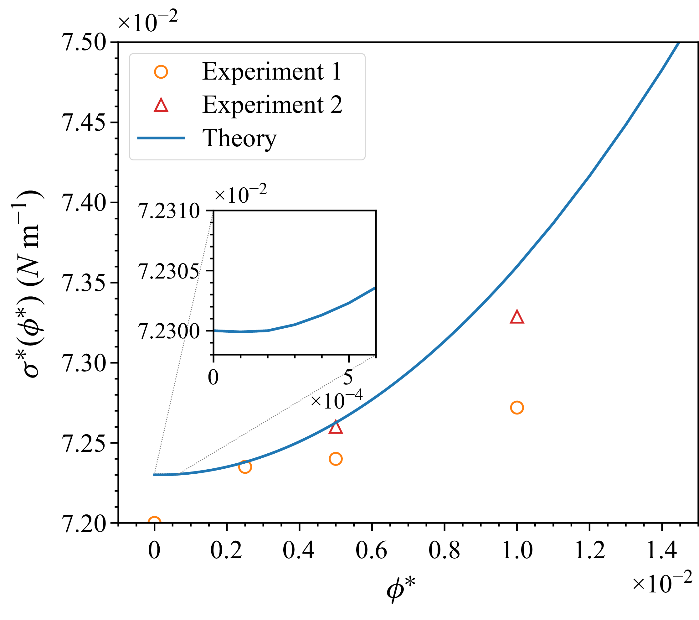


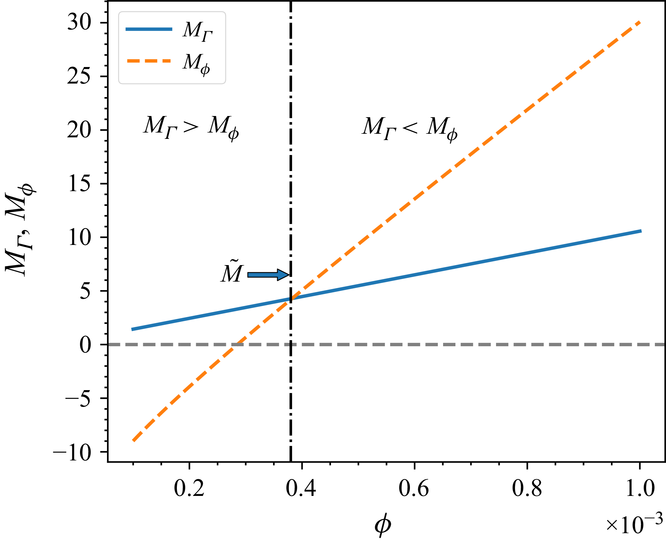


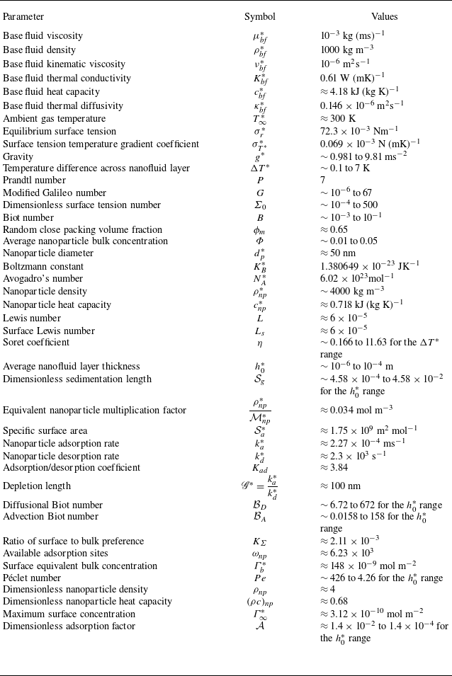
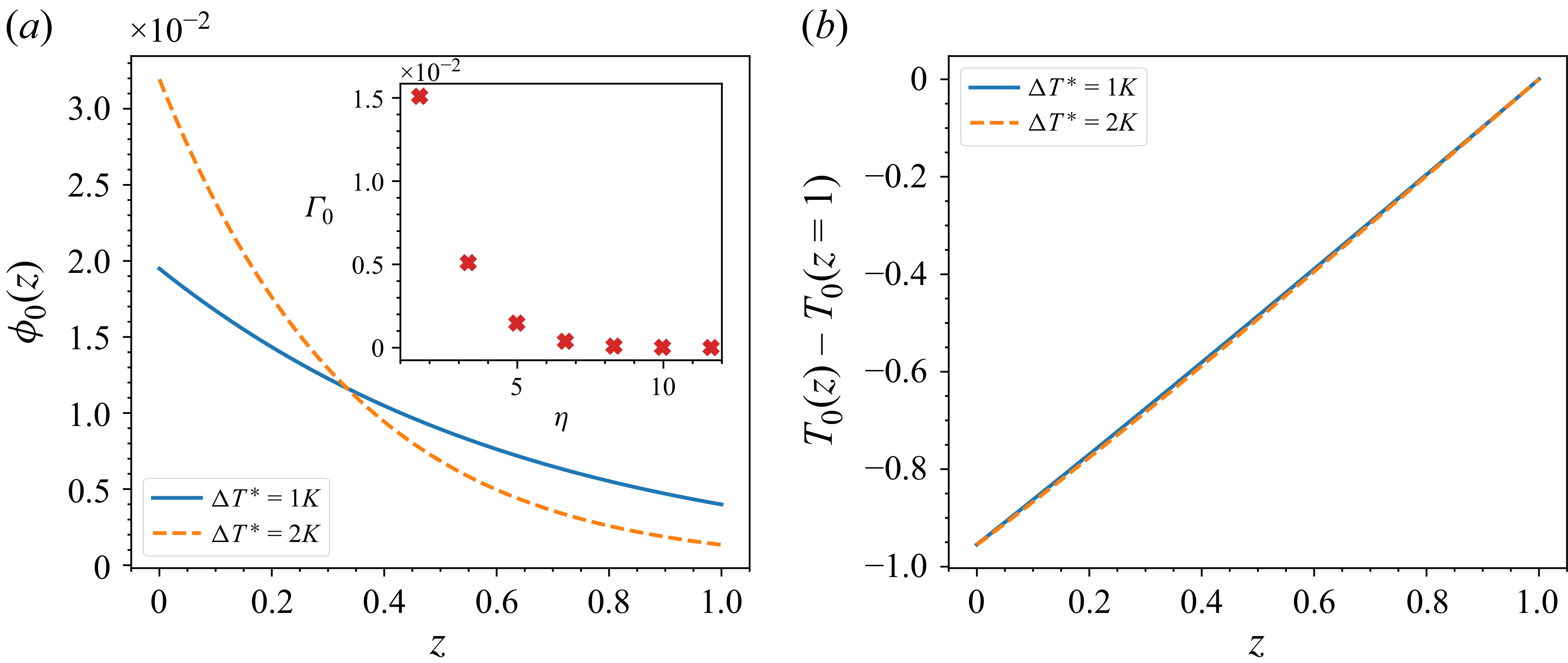


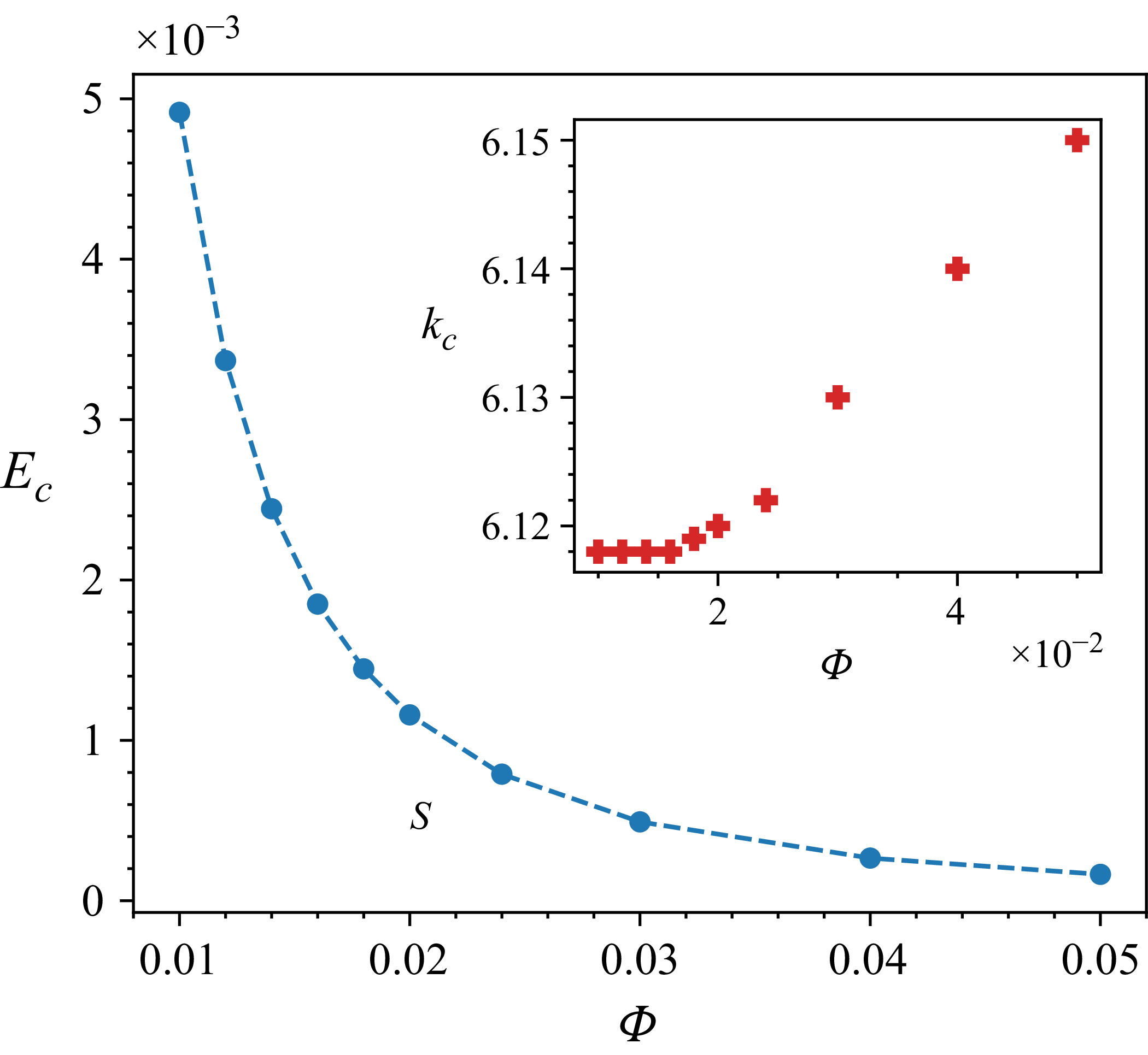


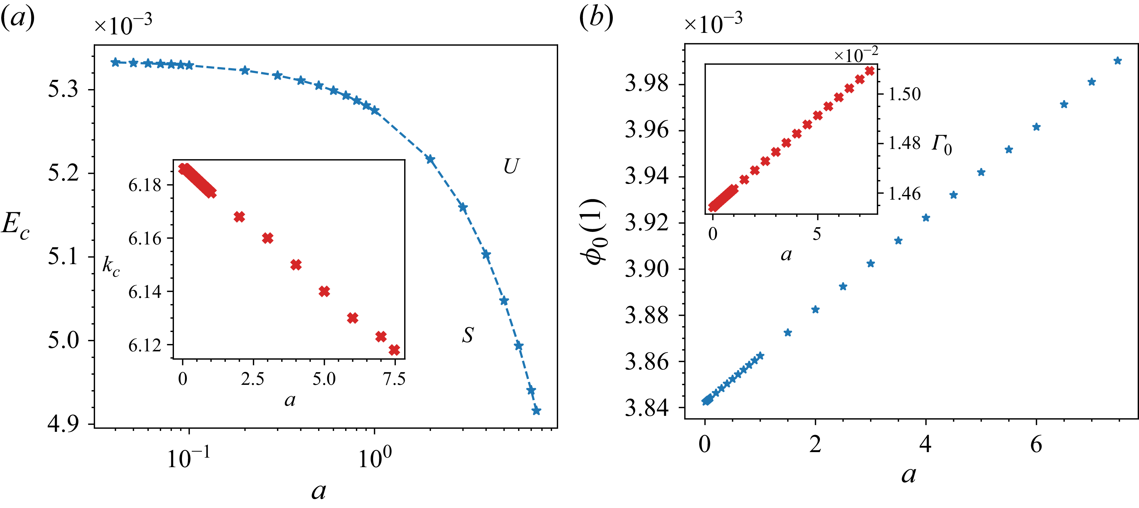


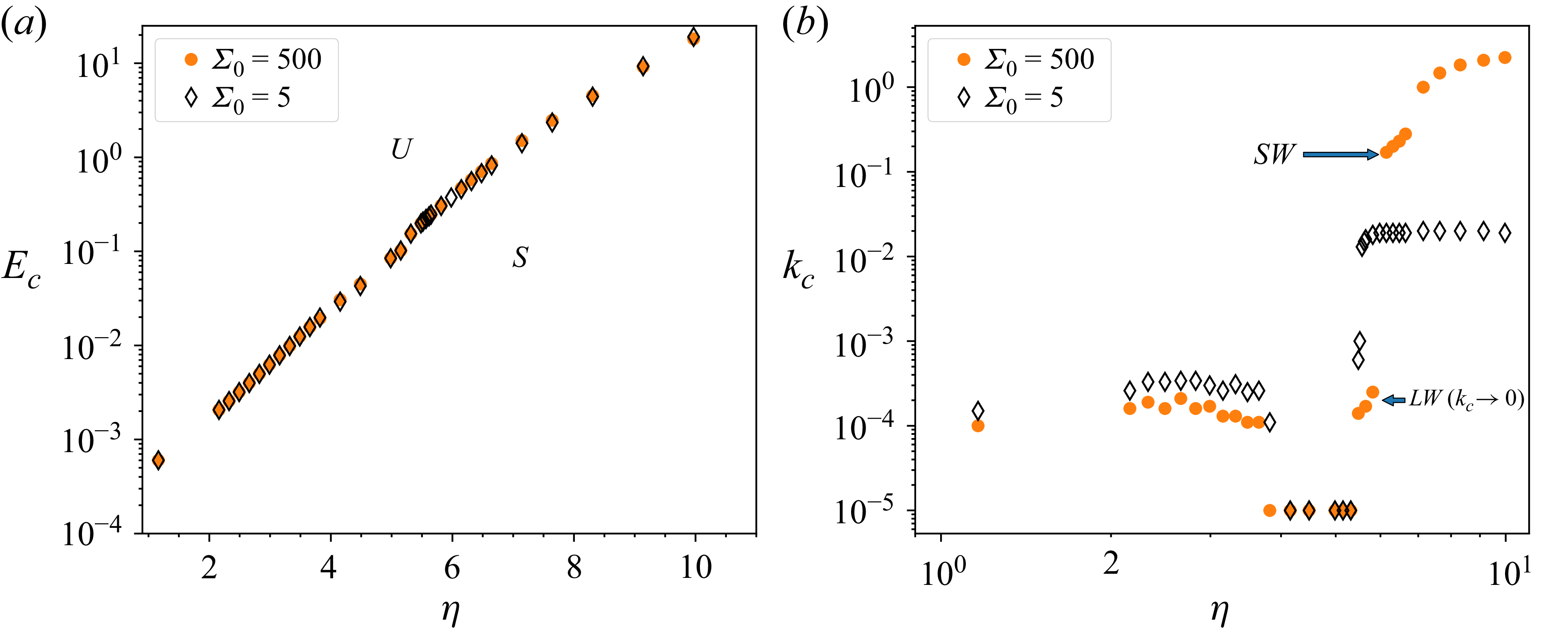


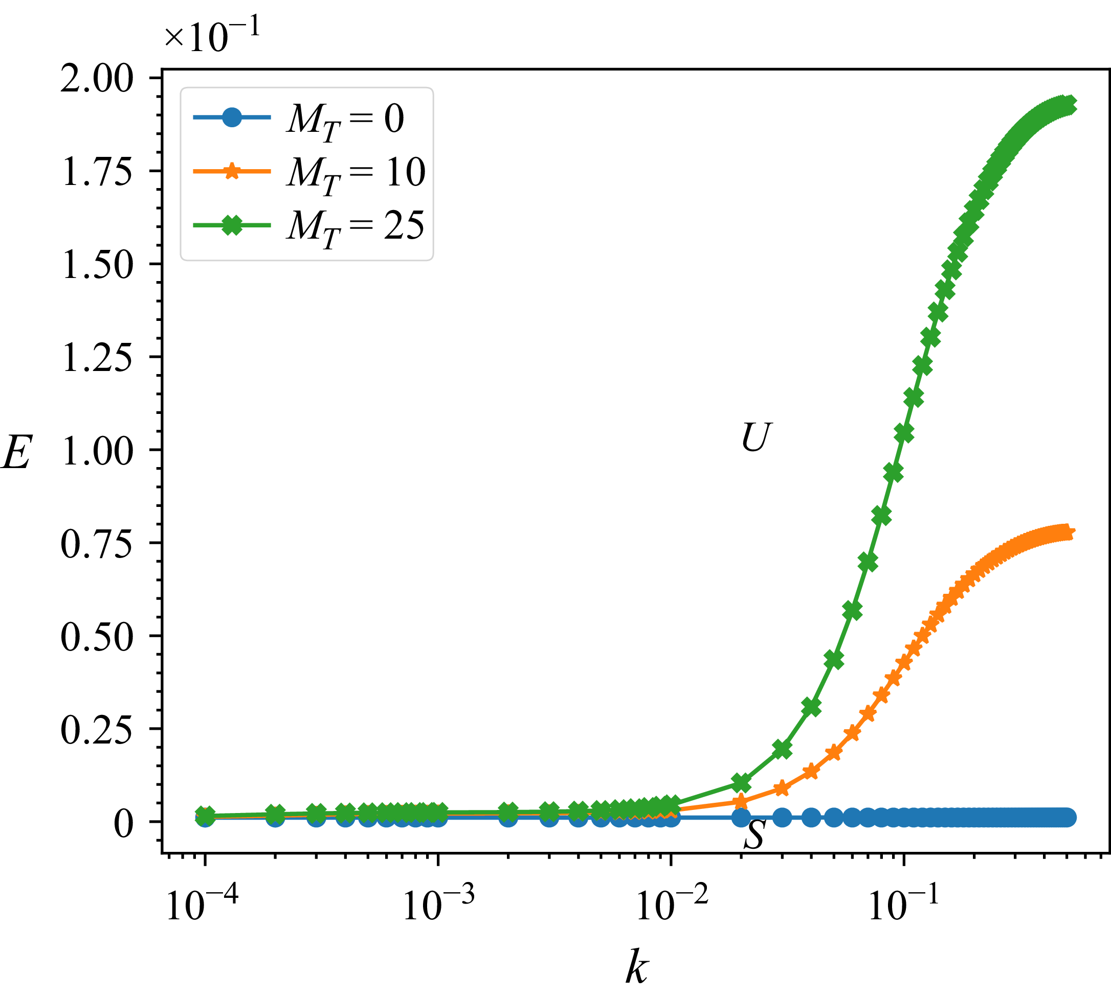


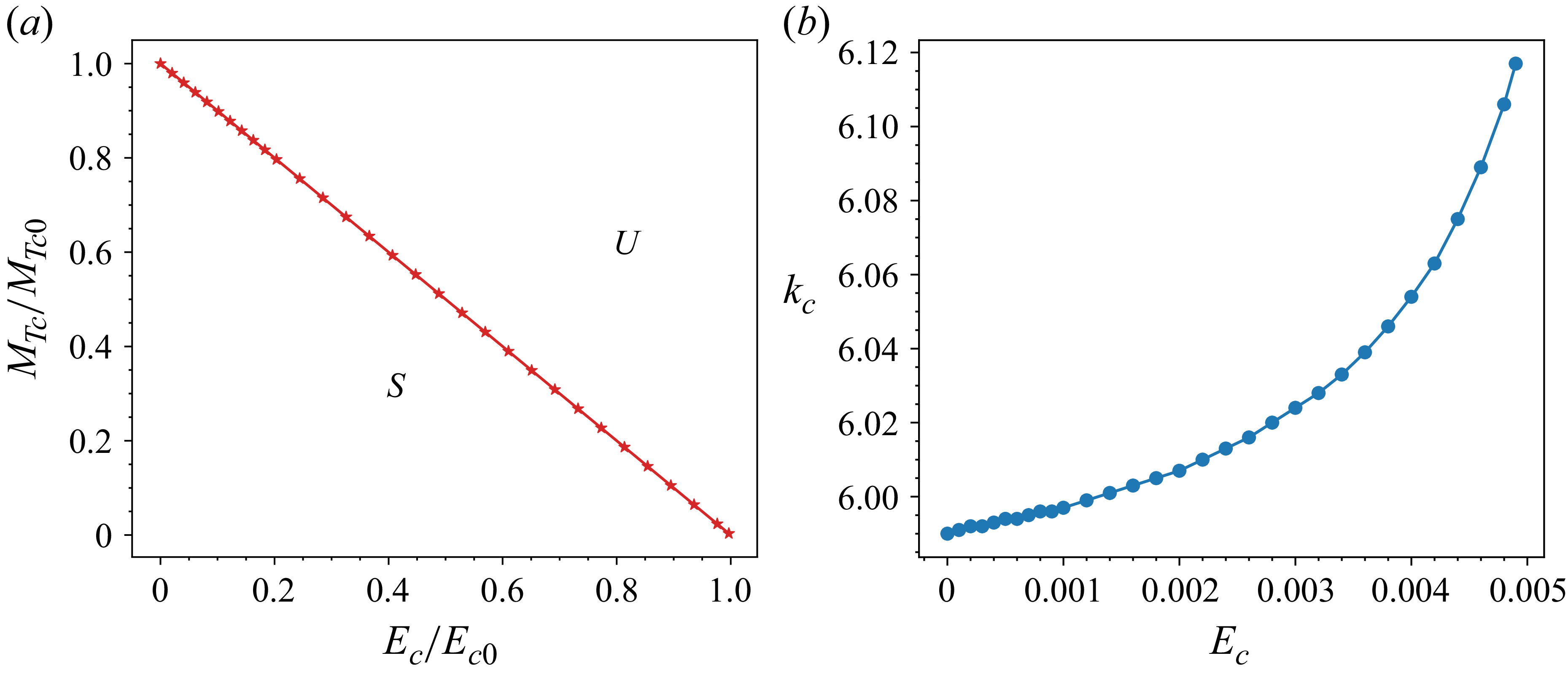


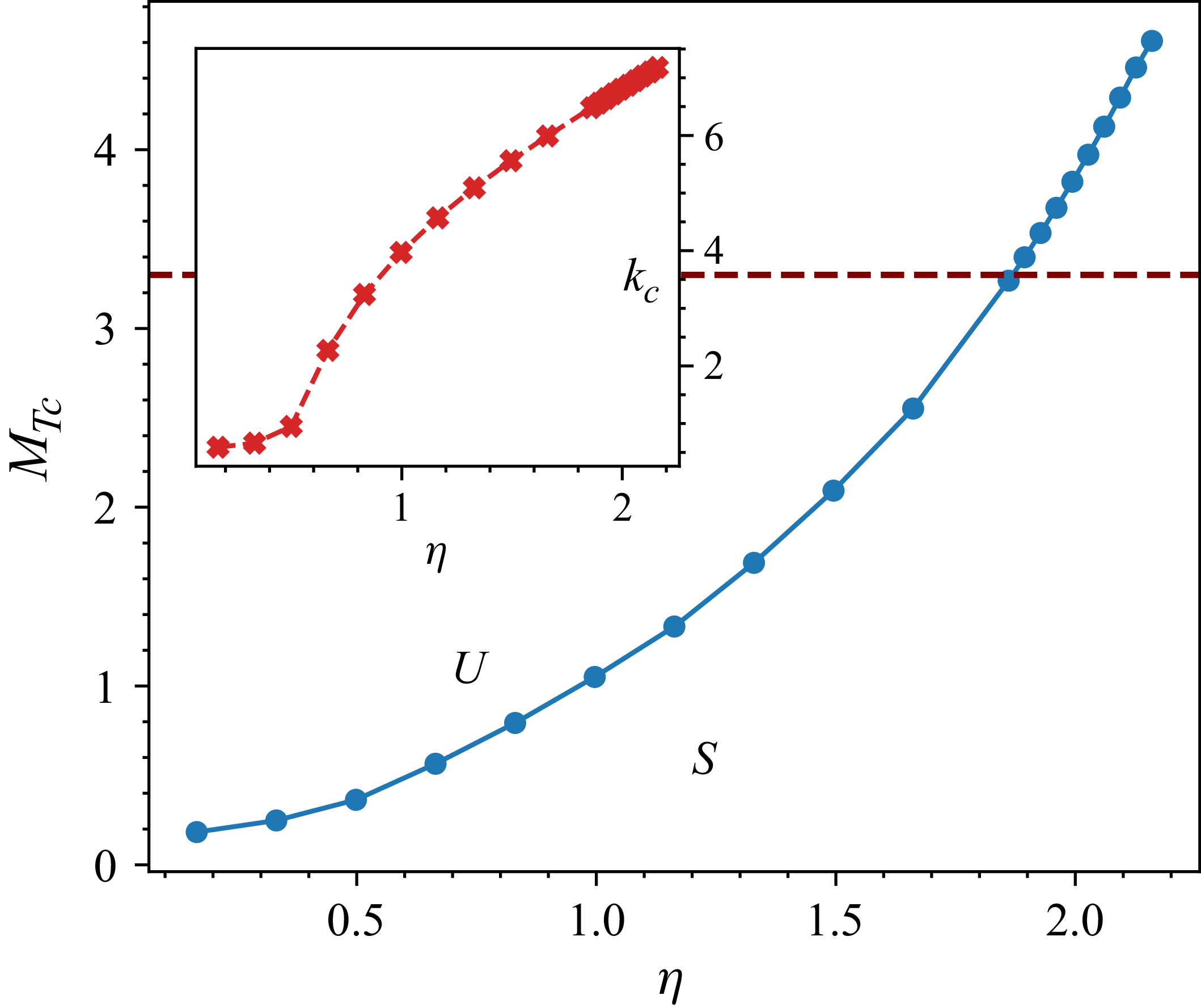


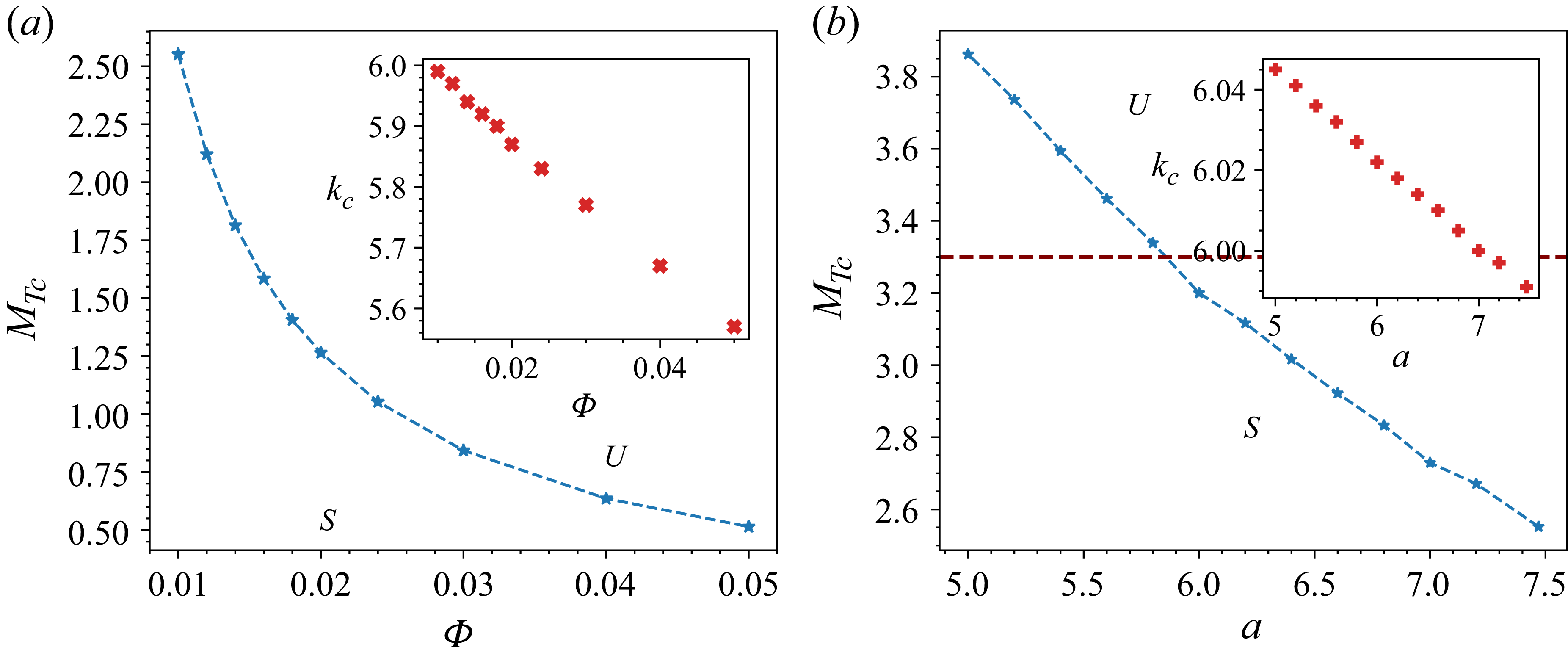


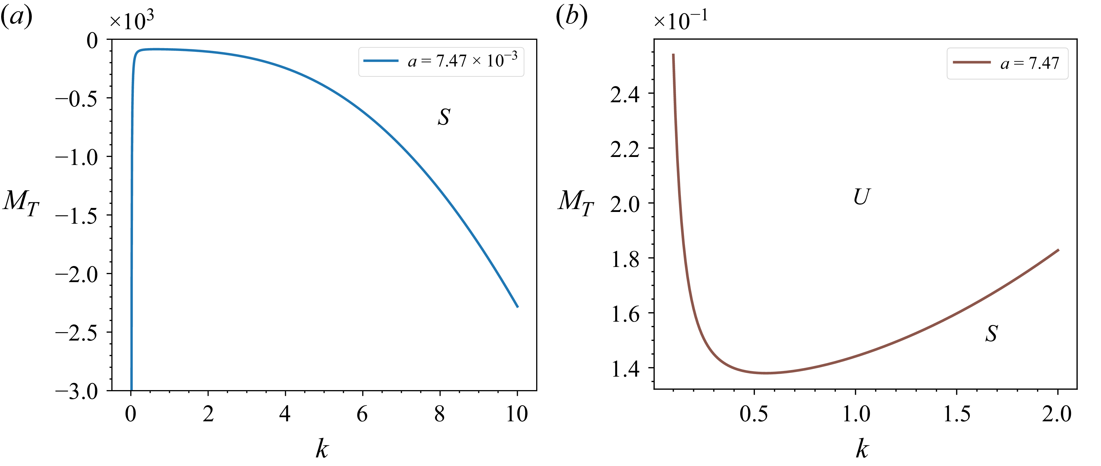


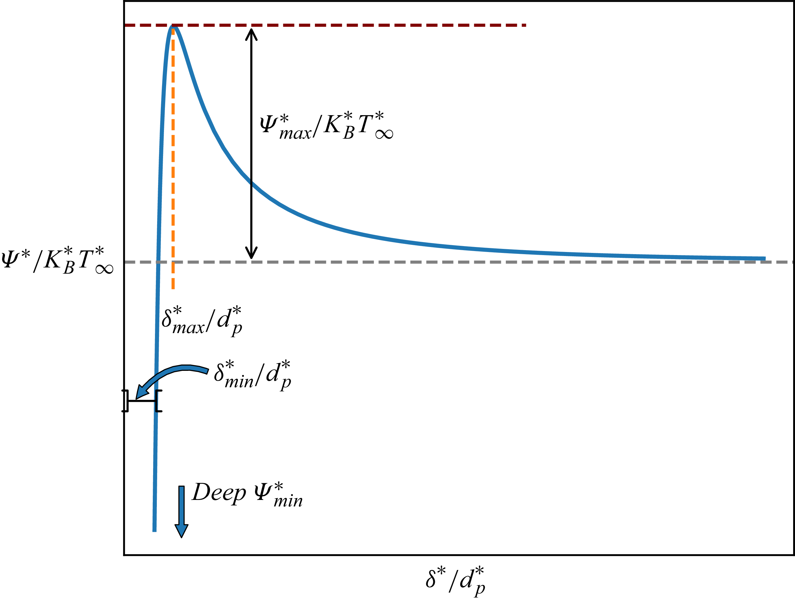


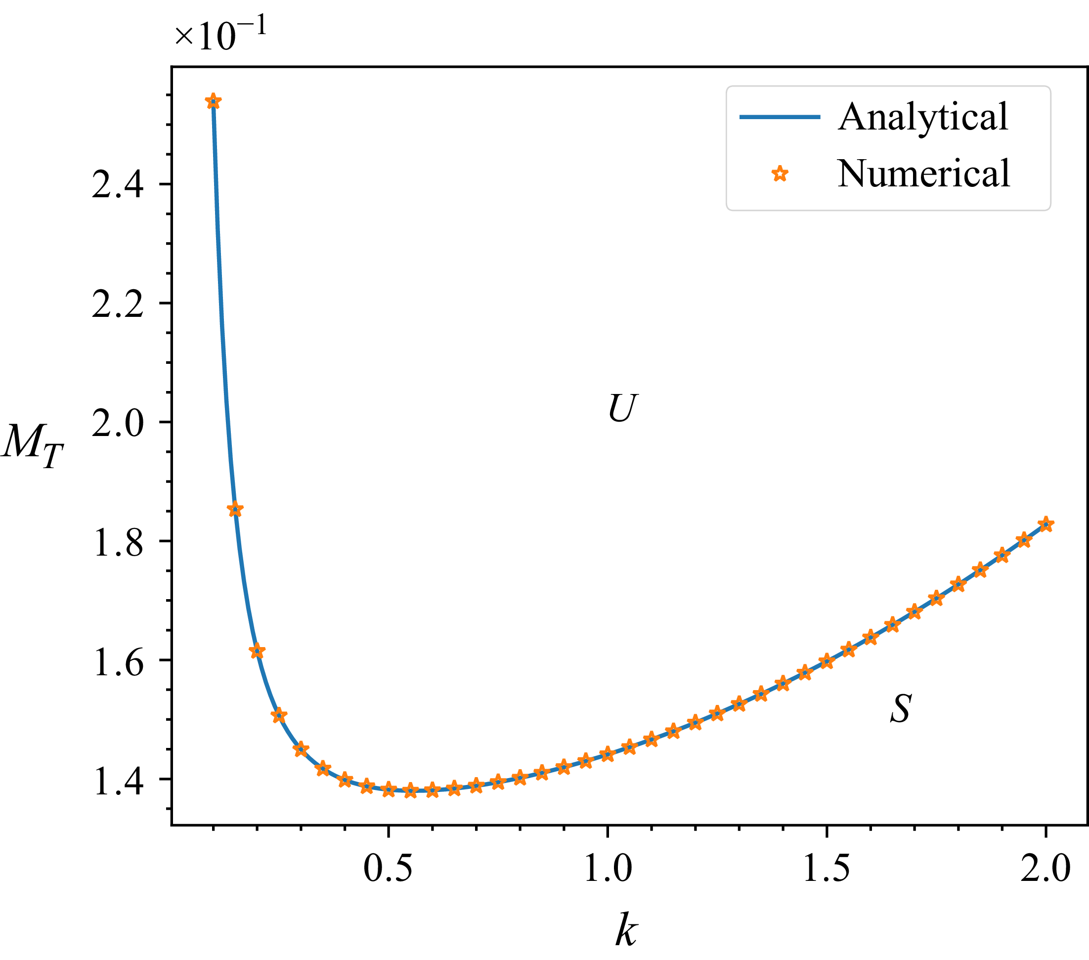


 Open access

